Bottlenecks CLUB:
Unifying Information-Theoretic Trade-offs Among
Complexity, Leakage, and Utility

Abstract

Bottleneck problems are an important class of optimization problems that have recently gained increasing attention in the domain of machine learning and information theory. They are widely used in generative models, fair machine learning algorithms, design of privacy-assuring mechanisms, and appear as information-theoretic performance bounds in various multi-user communication problems. In this work, we propose a general family of optimization problems, termed as complexity-leakage-utility bottleneck (CLUB) model, which (i) provides a unified theoretical framework that generalizes most of the state-of-the-art literature for the information-theoretic privacy models, (ii) establishes a new interpretation of the popular generative and discriminative models, (iii) constructs new insights to the generative compression models, and (iv) can be used in the fair generative models. We first formulate the CLUB model as a complexity-constrained privacy-utility optimization problem. We then connect it with the closely related bottleneck problems, namely information bottleneck (IB), privacy funnel (PF), deterministic IB (DIB), conditional entropy bottleneck (CEB), and conditional PF (CPF). We show that the CLUB model generalizes all these problems as well as most other information-theoretic privacy models. Then, we construct the deep variational CLUB (DVCLUB) models by employing neural networks to parameterize variational approximations of the associated information quantities. Building upon these information quantities, we present unified objectives of the supervised and unsupervised DVCLUB models. Leveraging the DVCLUB model in an unsupervised setup, we then connect it with state-of-the-art generative models, such as variational auto-encoders (VAEs), generative adversarial networks (GANs), as well as the Wasserstein GAN (WGAN), Wasserstein auto-encoder (WAE), and adversarial auto-encoder (AAE) models through the optimal transport (OT) problem. We then show that the DVCLUB model can also be used in fair representation learning problems, where the goal is to mitigate the undesired bias during the training phase of a machine learning model. We conduct extensive quantitative experiments on colored-MNIST and CelebA datasets, with a public implementation available, to evaluate and analyze the CLUB model.

1 Introduction

1.1 Motivation

Releasing an ‘optimal’ representation of data for a given task while simultaneously assuring privacy of the individuals’ identity and their associated data is an important challenge in today’s highly connected and data-driven world, and has been widely studied in the information theory, signal processing, data mining and machine learning communities. An optimal representation is the most useful (sufficient), compressed (compact), and least privacy-breaching (minimal) representation of data. Indeed, an optimal representation of data can be obtained subject to constraints on the target task and its computational and storage complexities.

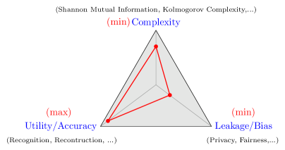
Figure 2: The schematic diagram of the trade-off among complexity, leakage and utility.

We investigate the problem of privacy-preserving data representation for a specific utility task, e.g., classification, identification, or reconstruction. Treating utility and privacy in a statistical framework [1] with mutual information as both the utility and obfuscation measures, we generalize the privacy funnel (PF) [2] and information bottleneck (IB) [3] models, and introduce a new and more general model called complexity-leakage-utility bottleneck (CLUB). Consider two parties, a data owner and a utility service provider. The data owner observes a random variable $\mathbf{X}$ and acquires some utility from the service provider based on the information he discloses. Simultaneously, the data owner wishes to limit the amount of information revealed about a sensitive random variable $\mathbf{S}$ that depends on $\mathbf{X}$. Therefore, instead of revealing $\mathbf{X}$ directly to the service provider, the data owner releases a new representation, denoted by $\mathbf{Z}$. The amount of information leaked to the service provider (public domain) about the sensitive variable $\mathbf{S}$ is measured by the mutual information $\mathrm{I}\left(\mathbf{S};\mathbf{Z}\right)$. Moreover, the data owner is subjected to a constraint on information complexity of representation that is revealed to the service provider. This imposed information complexity is measured by $\mathrm{I}\left(\mathbf{X};\mathbf{Z}\right)$. Moreover, in general, the acquired utility depends on a utility random variable $\mathbf{U}$ that is dependent on $\mathbf{X}$ and may also be correlated with $\mathbf{S}$. The amount of useful information revealed to the service provider is measured by $\mathrm{I}\left(\mathbf{U};\mathbf{Z}\right)$. Therefore, considering a Markov chain $\left(\mathbf{U},\mathbf{S}\right)\hbox{$\--$}\kern-1.5pt\hbox{$\circ$}\kern-1.5pt\hbox{$\--$}\mathbf{X}\hbox{$\--$}\kern-1.5pt\hbox{$\circ$}\kern-1.5pt\hbox{$\--$}\mathbf{Z}$, our aim is to share a privacy-preserving (sanitized) representation $\mathbf{Z}$ of observed data $\mathbf{X}$, through a stochastic mapping $P_{\mathbf{Z}\mid\mathbf{X}}$, while preserving information about utility attribute $\mathbf{U}$ and obfuscating information about sensitive attribute $\mathbf{S}$. The stochastic mapping $P_{\mathbf{Z}\mid\mathbf{X}}$ is called complexity-constrained obfuscation-utility-assuring mapping. The general diagram of our setup is depicted in Fig. 1. The schematic diagram of the trade-off among complexity, leakage and utility is depicted in Fig. 2.

1.2 Contributions

• Inspired by [4], we propose the CLUB model and provide a characterization of the complexity-leakage-utility trade-off for this model. The CLUB model provides a statistical inference framework that generalizes most of the state-of-the-art literature in the information-theoretic privacy models. To the best of our knowledge, this is the first unified formulation, which can bridge machine-learning and information-theoretic privacy communities.

• We provide new insights into the representation learning problems by bridging information-theoretic privacy with the generative models through the bottleneck principle. We start from a purely information-theoretic framework that has roots in the classical Shannon rate-distortion theory. Next we demonstrate the connection of our model to several recent research trends in generative models and representation learning. In particular, we show that the CLUB model has connections to the variational fair auto-encoder (VFAE) model [5] to learn representations for a prediction problem while removing potential biases against some variable (e.g., gender, ethnicity) from the results of a learned model [6, 7, 8, 9, 5, 10, 11, 12, 13, 14].

• We generalize the CLUB perspective to comprise both supervised and unsupervised setups. In the supervised setup, $\mathbf{U}$ is a generic attribute of data $\mathbf{X}$, while in the unsupervised setup, the data owner wishes to release the original domain data $\mathbf{X}$ (e.g., facial images) as accurately as possible (i.e., $\mathbf{U}\equiv\mathbf{X}$), without revealing a specific sensitive attribute $\mathbf{S}$ (e.g., gender, emotion, etc.). In the unsupervised setup, the deep variational CLUB (DVCLUB) model is shown to have interesting connections with the several generative models such as variational auto-encoder (VAE) [15], $\beta$-VAE [16], InfoVAE [17], generative adversarial network (GAN) [18], Wasserstein GAN (WGAN) [19], Wasserstein auto-encoders [20], adversarial auto-encoder (AAE) [21], VAE-GAN [22], and BIB-AE [23].

• We conduct extensive qualitative and quantitative experiments on several real-world datasets to evaluate and validate the effectiveness of the proposed CLUB model.

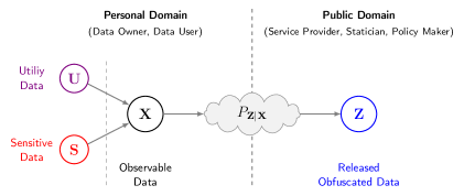
Figure 1: The general complexity-leakage-utility bottleneck framework.

1.3 State-of-the-Art

Addressing data anonymization in [24], various well-known statistical formulations and schemes were proposed for preserving-privacy of data, such as $k$-anonymity [25], $\ell$-diversity [26], $t$-closeness [27], differential privacy (DP) [28], and pufferfish [29], which are basically based on some form of data perturbation. These mechanisms mainly focus on the querying data, inference algorithms and transporting probability measures. DP is the most popular context-free notion of privacy, which is characterized in terms of the distinguishability of ‘neighboring’ databases. However, DP does not provide any guarantee on the (average or maximum) information leakage [1]. Pufferfish framework is a generalized version of DP that can capture data correlation; however, it does not focus on preserving data utility.

Information theoretic (IT) privacy approaches [30, 31, 32, 33, 1, 34, 35, 36, 37, 38, 39, 40, 41, 42, 43, 44, 45, 46, 47, 48, 49, 50, 51, 52, 53, 54, 55, 56] model and analyze privacy-utility trade-offs using IT metrics to provide asymptomatic or non-asymptotic privacy-utility-guarantees. Following Shannon’s information-theoretic notion of secrecy [57], where security is measured through the equivocation rate at the eavesdropper, Reed [30] and Yamamoto [31] treated security and privacy from a lossy source coding standpoint, i.e., from the rate-distortion theory. Inspired by [31], in the most general form, the IT privacy framework is based on the presence of a specific ‘private’ variable (or attribute, information) and a correlated non-private variable, and the knowledge of exact joint distribution or partial statistical knowledge of private and/or non-private variables. In this setup, the goal is to design a privacy assuring mapping that transforms the pair of these variables into a new representation that achieves a specific application-based target utility, while simultaneously minimizing the information inferred about the private variable. Although IT privacy approaches provide context-aware notion of privacy, which can explicitly model the capability of data users and adversaries, it requires statistical knowledge of data, i.e., priors.

Inspired by GANs [18], the recent data-driven privacy mechanisms address the privacy-utility trade-off as a constrained mini-max game between two players: a defender (privatizer) that encodes the dataset to minimize the inference leakage on the individual’s private/sensitive variables, and an adversary that tries to infer the ‘private’ variables from the released dataset [58, 59, 60, 48, 61]. The adversarial training algorithms proposed in [58, 59], considered deterministic approaches for optimizing privacy-preserving mechanisms. The authors in [60] and [48], independently and simultaneously, addressed randomness in their training algorithms. Our model subsumes these models. We establish a more precise connection with the state-of-the-art after introducing the CLUB model.

Our model is inspired by [4], where the authors established the rate region of the extended Gray-Wyner system for two discrete memoryless sources, which include Wyner’s common information, Gács-Körner common information, IB, Körner graph entropy, necessary conditional entropy, and the PF, as extreme points. We extend and unify most of the previously proposed objectives in the state-of-the-art literature based on IT privacy models. We hope that our unified model can serve as a reference for researchers and practitioners interested in designing privacy-sensitive data release mechanisms. Our research is also closely related to [62, 51, 63, 64]. Considering the Markov chain $\left(\mathbf{U},\mathbf{S}\right)\hbox{$\--$}\kern-1.5pt\hbox{$\circ$}\kern-1.5pt\hbox{$\--$}\mathbf{X}\hbox{$\--$}\kern-1.5pt\hbox{$\circ$}\kern-1.5pt\hbox{$\--$}\mathbf{Z}$, the authors in [62] addressed the problem of privacy-preserving representation learning in a scenario where the goal is to share a sanitized representation $\mathbf{Z}$ of high-dimensional data $\mathbf{X}$ while preserving information about utility attribute $\mathbf{U}$ and obfuscate information about private (sensitive) attribute $\mathbf{S}$. Inspired by GANs, the framework is formulated as a distribution matching problem. Compared with [62], our formulation is more general as it addresses a key missing component in their formulation, i.e., the rate (description length, information complexity) constraint. Another fundamental related work to ours is [51], which studied the rate-constrained privacy-utility trade-off problem and considered a similar model as [62], independently. The proposed framework is restricted to discrete alphabets and studied the necessary and sufficient conditions for the existence of positive utility, i.e., $\mathrm{I}(U;Z)>0$, under a perfect obfuscation regime, i.e., $\mathrm{I}(S;Z)=0$. Analogous to [51], considering the Markov chain $\left(U,S\right)\hbox{$\--$}\kern-1.5pt\hbox{$\circ$}\kern-1.5pt\hbox{$\--$}X\hbox{$\--$}\kern-1.5pt\hbox{$\circ$}\kern-1.5pt\hbox{$\--$}Z$, the authors in [63] adopted a local information geometry analysis to construct the modal decomposition of the joint distributions, divergence transfer matrices, and mutual information. Next, they obtained the locally sufficient statistics for inferences about the utility attribute, while satisfying perfect obfuscation constraint. Furthermore, they developed the notion of perfect obfuscation based on $\chi^{2}$-divergence and Kullback–Leibler divergence in the Euclidean information space. Considering the Markov chain $\left(\mathbf{U},\mathbf{S}\right)\hbox{$\--$}\kern-1.5pt\hbox{$\circ$}\kern-1.5pt\hbox{$\--$}\mathbf{X}\hbox{$\--$}\kern-1.5pt\hbox{$\circ$}\kern-1.5pt\hbox{$\--$}\mathbf{Z}$, the role of information complexity in privacy leakage about an attribute of an adversary’s interest is studied in [64]. In contrast to the PF and generative adversarial privacy models, they considered the setup in which the adversary’s interest is not known a priori to the data owner. More detailed connections between the CLUB model and the state-of-the-art bottleneck models, generative models, modern data compression models, and fair machine learning models is presented in Sec. 6.

1.4 Outline

In Sec. 2, we present the general problem statement of the CLUB model, and next we briefly review and introduce a few preliminary concepts that are necessary to understand the problem formulation. We then present the CLUB model in Sec. 3. The variational bounds of information measures are derived in Sec. 4. The DVCLUB model is presented in Sec. 5. More detailed connections between the CLUB model and the literature is presented in Sec. 6. Experimental results are provided in Sec. 7. Finally, conclusions are drawn in Sec. 8.

1.5 Notations

Throughout this paper, random variables are denoted by capital letters (e.g., $X$, $Y$), deterministic values are denoted by small letters (e.g., $x$, $y$), random vectors are denoted by capital bold letter (e.g., $\mathbf{X}$, $\mathbf{Y}$), deterministic vectors are denoted by small bold letters (e.g., $\mathbf{x}$, $\mathbf{y}$), alphabets (sets) are denoted by calligraphic fonts (e.g., $\mathcal{X,Y}$), and for specific quantities/values we use sans serif font (e.g., $\mathsf{x}$, $\mathsf{y}$, $\mathsf{C}$, $\mathsf{D}$, $\mathsf{P}$, $\Omega)$. Superscript $(.)^{T}$ stands for the transpose. Also, we use the notation $\left[N\right]$ for the set $\{1,2,3,...,N\}$. $\mathrm{H}\left(P_{\mathbf{X}}\right)\coloneqq\mathbb{E}_{P_{\mathbf{X}}}\left[-\log P_{\mathbf{X}}\right]$ denotes the Shannon entropy; $\mathrm{H}\left(P_{\mathbf{X}}\|Q_{\mathbf{X}}\right)\coloneqq\mathbb{E}_{P_{\mathbf{X}}}\left[-\log Q_{\mathbf{X}}\right]$ denotes the cross-entropy of the distribution $P_{\mathbf{X}}$ relative to a distribution $Q_{\mathbf{X}}$; and $\mathrm{H}\left(P_{\mathbf{Z}\mid\mathbf{X}}\|Q_{\mathbf{Z}\mid\mathbf{X}}\mid P_{\mathbf{X}}\right)\coloneqq\mathbb{E}_{P_{\mathbf{X}}}\mathbb{E}_{P_{\mathbf{Z}\mid\mathbf{X}}}\left[-\log Q_{\mathbf{Z}\mid\mathbf{X}}\right]$ denotes the cross-entropy loss for $Q_{\mathbf{Z}\mid\mathbf{X}}$. The relative entropy is defined as $\mathrm{D}_{\mathrm{KL}}\left(P_{\mathbf{X}}\|Q_{\mathbf{X}}\right)\coloneqq\mathbb{E}_{P_{\mathbf{X}}}\big{[}\log\frac{P_{\mathbf{X}}}{Q_{\mathbf{X}}}\big{]}$. The conditional relative entropy is defined by $\mathrm{D}_{\mathrm{KL}}\left(P_{\mathbf{Z}\mid\mathbf{X}}\|Q_{\mathbf{Z}\mid\mathbf{X}}\mid P_{\mathbf{X}}\right)\coloneqq\mathbb{E}_{P_{\mathbf{X}}}\left[\mathrm{D}_{\mathrm{KL}}\left(P_{\mathbf{Z}\mid\mathbf{X}=\mathbf{x}}\|Q_{\mathbf{Z}\mid\mathbf{X}=\mathbf{x}}\right)\right]$ and the mutual information is defined by $\mathrm{I}\left(P_{\mathbf{X}};P_{\mathbf{Z}\mid\mathbf{X}}\right)\coloneqq\mathrm{D}_{\mathrm{KL}}\left(P_{\mathbf{Z}\mid\mathbf{X}}\|P_{\mathbf{Z}}\mid P_{\mathbf{X}}\right)$. We abuse notation to write $\mathrm{H}\left(\mathbf{X}\right)=\mathrm{H}\left(P_{\mathbf{X}}\right)$ and $\mathrm{I}\left(\mathbf{X};\mathbf{Z}\right)=\mathrm{I}\left(P_{\mathbf{X}};P_{\mathbf{Z}\mid\mathbf{X}}\right)$ for random objects $\mathbf{X}\sim P_{\mathbf{X}}$ and $\mathbf{Z}\sim P_{\mathbf{Z}}$. We use the same notation for the probability distributions and the associated densities.

2 Problem Statement and Preliminaries

In this section, first we present the general problem statement of the CLUB model, and next we introduce the main concepts necessary to understand the fundamentals of our model. In particular, we concretely express our inference threat model and explain why we consider mutual information as the obfuscation and utility measures. Next, we briefly address the concepts of relevant information and minimal sufficient statistics.

2.1 General Problem Statement

Consider the problem of releasing a sanitized representation $\mathbf{Z}$ of observed data $\mathbf{X}$, through a stochastic mapping $P_{\mathbf{Z}\mid\mathbf{X}}$, while preserving information about a utility attribute $\mathbf{U}$ and obfuscating a sensitive attribute $\mathbf{S}$. In this scenario, $\left(\mathbf{U},\mathbf{S}\right)\hbox{$\--$}\kern-1.5pt\hbox{$\circ$}\kern-1.5pt\hbox{$\--$}\mathbf{X}\hbox{$\--$}\kern-1.5pt\hbox{$\circ$}\kern-1.5pt\hbox{$\--$}\mathbf{Z}$ forms a Markov chain. In general, one can consider a well-defined generic obfuscation measure as a functional of the joint distribution $P_{\mathbf{S},\mathbf{Z}}$ that captures the amount of leakage about $\mathbf{S}$ by releasing $\mathbf{Z}$. Let $\mathcal{C}_{\mathsf{L}}:\mathcal{P}\left(\mathcal{S}\times\mathcal{Z}\right)\rightarrow\mathbb{R}^{+}\cup\{0\}$ denote this generic leakage (obfuscation) measure. On the other hand, one can consider a well-defined and application-specific generic utility measure as a functional of the joint distribution $P_{\mathbf{U},\mathbf{Z}}$ that captures the amount of utility about $\mathbf{U}$ by releasing $\mathbf{Z}$, instead of original data $\mathbf{X}$. Let $\mathcal{C}_{\mathsf{U}}:\mathcal{P}\left(\mathcal{U}\times\mathcal{Z}\right)\rightarrow\mathbb{R}^{+}\cup\{0\}$ denote a generic utility loss measure. Finally, let $\mathcal{C}_{\mathsf{C}}:\mathcal{P}\left(\mathcal{X}\times\mathcal{Z}\right)\rightarrow\mathbb{R}^{+}\cup\{0\}$ denote a generic measure of complexity of the distribution $P_{\mathbf{Z}\mid\mathbf{X}}$ for the data distribution $P_{\mathbf{X}}$. Then, one can consider the generic CLUB functional as:

$$\mathsf{CLUB}\left(P_{\mathbf{U},\mathbf{S},\mathbf{X}}\right)\coloneqq\mathop{\inf}_{\begin{subarray}{c}P_{\mathbf{Z}\mid\mathbf{X}}:\\ \left(\mathbf{U},\mathbf{S}\right)\hbox{$\--$}\kern-1.5pt\hbox{$\circ$}\kern-1.5pt\hbox{$\--$}\mathbf{X}\hbox{$\--$}\kern-1.5pt\hbox{$\circ$}\kern-1.5pt\hbox{$\--$}\mathbf{Z}\end{subarray}}\mathcal{C}_{\mathsf{C}}\left(P_{\mathbf{X}},P_{\mathbf{Z}\mid\mathbf{X}}\right)+\mathcal{C}_{\mathsf{L}}\left(P_{\mathbf{S}},P_{\mathbf{Z}\mid\mathbf{X}}\right)+\mathcal{C}_{\mathsf{U}}\left(P_{\mathbf{U}},P_{\mathbf{Z}\mid\mathbf{X}}\right).$$ (1)

2.2 Obfuscation and Utility Measures under Logarithmic Loss

We consider obfuscation-utility trade-off model where both utility and obfuscation are measured under logarithmic loss (also often referred to as the self-information loss). The logarithmic loss function has been widely used in learning theory [65], image processing [66], IB [67], multi-terminal source coding [68], as well as PF [2]. In this case, both the obfuscation and utility measures can be modelled by the mutual information. By minimizing the obfuscation measure under the logarithmic loss, one actually minimizes an upper bound on any bounded loss function [2].

Consider the inference threat model introduced in [1], which models a broad class of adversaries that perform statistical inference attacks on the sensitive data. Consider an inference cost function $\mathsf{C}:\mathcal{S}\times\mathcal{P}\left(\mathcal{S}\right)\rightarrow\mathbb{R}^{+}\cup\{0\}$. Prior to observing $\mathbf{Z}$, the adversary chooses a belief distribution $Q$ from the set $\mathcal{P}\!\left(\mathcal{S}\right)$ of all possible distributions over $\mathcal{S}$, that minimizes the expected inference cost function $\mathsf{C}\left(\mathbf{S},Q\right)$. Therefore:

$$Q^{\ast}=\arg\mathop{\min}_{Q\in\mathcal{P}\left(\mathcal{S}\right)}\mathbb{E}_{P_{\mathbf{S}}}\left[\mathsf{C}\left(\mathbf{S},Q\right)\right].$$ (2)

Let $c_{0}^{\ast}=\mathbb{E}_{P_{\mathbf{S}}}\left[\mathsf{C}\left(\mathbf{S},Q^{\ast}\right)\right]$ denote the corresponding minimum average cost. After observing $\mathbf{Z}=\mathbf{z}$, the adversary revises his belief distribution as:

$$Q_{\mathbf{z}}^{\ast}=\arg\mathop{\min}_{Q\in\mathcal{P}\left(\mathcal{S}\right)}\mathbb{E}_{P_{\mathbf{S}\mid\mathbf{Z}}}\left[\mathsf{C}\left(\mathbf{S},Q\right)\mid\mathbf{Z}=\mathbf{z}\right].$$ (3)

Let $c_{\mathbf{z}}^{\ast}=\mathbb{E}_{P_{\mathbf{S\mid Z}}}\left[\mathsf{C}\left(\mathbf{S},Q_{\mathbf{z}}^{\ast}\right)\right]$ denote the corresponding minimum average cost of inferring $\mathbf{S}$ after observing $\mathbf{Z=z}$. Therefore, the adversary obtains an average gain of $\Delta\mathsf{C}=c_{0}^{\ast}-\mathbb{E}_{P_{\mathbf{Z}}}\left[c_{\mathbf{Z}}^{\ast}\right]$ in inference cost. This cost gain measures the improvement in the quality of the inference of sensitive data $\mathbf{S}$ due to observation of $\mathbf{Z}$. Under the self-information loss cost function $\mathsf{C}\left(\mathbf{s},Q\right)=-\log Q(\mathbf{s}),\forall\mathbf{s}\in\mathcal{S}$, the information leakage $\Delta\mathsf{C}$ can be measured by the Shannon mutual information $\mathrm{I}\left(\mathbf{S};\mathbf{Z}\right)$.

On the other hand, the stochastic mapping $P_{\mathbf{Z}\mid\mathbf{X}}$ should maintain the utility of desired data $\mathbf{U}$. Under the self-information loss, the utility measure is defined as $d\left(\mathbf{u},\mathbf{z}\right)=-\log P_{\mathbf{U}\mid\mathbf{Z}}\left(\mathbf{u}\mid\mathbf{z}\right)$, which is a function of $\mathbf{u}$ and $\mathbf{z}$ as well as stochastic mapping $P_{\mathbf{Z}\mid\mathbf{X}}$. Hence, the average utility loss is $\mathbb{E}_{P_{\mathbf{U},\mathbf{Z}}}\left[-\log P_{\mathbf{U}\mid\mathbf{Z}}\right]=\mathrm{H}\left(\mathbf{U}\mid\mathbf{Z}\right)$ that can be minimized by designing the stochastic mapping $P_{\mathbf{Z}\mid\mathbf{X}}$. Consider some utility level $E^{\mathrm{u}}\geq 0$, such that we constrain to have $\mathrm{H}\left(\mathbf{U}\mid\mathbf{Z}\right)\leq E^{\mathrm{u}}$. Given $P_{\mathbf{U}}$, and therefore $\mathrm{H}\left(\mathbf{U}\right)$, and assuming that $R^{\mathrm{u}}=\mathrm{H}(\mathbf{U})-E^{\mathrm{u}}\geq 0$, the utility constraint can be recast as $\mathrm{I}\left(\mathbf{U};\mathbf{Z}\right)\geq R^{\mathrm{u}}$.

In Sec. 3, built upon this general threat model and considering the self-information loss as both utility and obfuscation measures, we present a unified formulation for the complexity-leakage-utility trade-off that generalizes most of the state-of-the-art literature.

2.3 Relevant Information

The relevant information is a common concept in information theory and statistics which captures the information that a random object $\mathbf{X}$ contains about another random object $\mathbf{U}$. Below, we present statistical and information-theoretical formulations proposed for measuring relevant information.

Definition 1 (Sufficient Statistic).

Let $\mathbf{U}\in\mathcal{U}$ be an unknown parameter and $\mathbf{X}\in\mathcal{X}$ be a random variable with conditional probability distribution function $P_{\mathbf{X}\mid\mathbf{U}}$. Given a function $f:\mathcal{X}\rightarrow\mathcal{Z}$, the random variable $\mathbf{Z}=f(\mathbf{X})$ is called a sufficient statistics for $\mathbf{U}$ if and only if (iff) [69, 70]:

$$P_{\mathbf{X}\mid{\mathbf{U},\mathbf{Z}}}\,(\mathbf{x}\mid\mathbf{u},\mathbf{z})=P_{\mathbf{X}\mid{\mathbf{Z}}}\,(\mathbf{x}\mid\mathbf{z}),\;\;\forall(\mathbf{x},\mathbf{u})\in\mathcal{X}\times\mathcal{U}.$$ (4)

Equivalently, quantifying with mutual information, we have:

$$\mathrm{I}\left(\mathbf{U};\mathbf{Z}\right)=\mathrm{I}\left(\mathbf{U};\mathbf{X}\right).\vspace{-3pt}$$ (5)

Note that $\mathbf{U}\hbox{$\--$}\kern-1.5pt\hbox{$\circ$}\kern-1.5pt\hbox{$\--$}\mathbf{X}\hbox{$\--$}\kern-1.5pt\hbox{$\circ$}\kern-1.5pt\hbox{$\--$}f\!\left(\mathbf{X}\right)$ forms a Markov chain, and by the data processing inequity (DPI), for a general statistic $f\!\left(\mathbf{X}\right)$, we have $\mathrm{I}\left(\mathbf{U};f\!\left(\mathbf{X}\right)\right)\leq\mathrm{I}\left(f\!\left(\mathbf{X}\right);\mathbf{X}\right)$. If equality holds, a sufficient statistic $\mathbf{Z}$ captures all the information in $\mathbf{X}$ about $\mathbf{U}$.

Remark 1 (Measure-Theoretic Interpretation).

Consider a probability space $\left(\Omega,\mathcal{B},\mathsf{P}\right)$, where $\mathcal{B}$ denotes the $\sigma$-algebra of all subsets of $\Omega$, and $\mathsf{P}$ is a probability measure defined on the measurable space $\left(\Omega,\mathcal{B}\right)$. Given two measurable spaces $\left(\Omega,\mathcal{B}\right)$ and $\left(\mathcal{X},\mathcal{F}\right)$, a random object (or measurable space) is a mapping (or function) $X:\Omega\rightarrow\mathcal{X}$, i.e., a measurable function defined on $\left(\Omega,\mathcal{B}\right)$ and taking values in $\left(\mathcal{X},\mathcal{F}\right)$, with the property that if $\mathpzc{E}\in\mathcal{F}$, then $X^{-1}\left(\mathpzc{E}\right)=\{\omega:X(\omega)\in\mathpzc{E}\}\in\mathcal{B}$. In this case, this random object is also called $\mathcal{F}$-measurable. Let $\mathcal{Z}$ be a proper subset of $\mathcal{X}$. A sufficient statistic is defined to be a measurable mapping $f$ from the measurable space $\left(\mathcal{X},\mathcal{F}\right)$ onto a measurable space $\left(\mathcal{Z},\mathcal{A}_{f}\right)$, i.e., $f:\left(\mathcal{X},\mathcal{F}\right)\rightarrow\left(\mathcal{Z},\mathcal{A}_{f}\right)$. The classical problem of data reduction is to find a partition $\mathcal{A}_{f}$ of $\mathcal{X}$ determined by some measurable mapping $f$. In other words, the problem is to find a new random object $Z\left(\omega\right)=f\left(X\left(\omega\right)\right)$.

Remark 2 (Simple Interpretation).

A statistic $\mathbf{Z}=f\!\left(\mathbf{X}\right)$ induces a partition on sample space $\mathcal{X}$. For each $\mathbf{Z}=\mathbf{z}$, the sample set $\{\mathbf{x}:f(\mathbf{x})=\mathbf{z}\}$ is one element of the partition, i.e., $\mathbf{z}\in\mathcal{Z}=\{\mathbf{z}:\mathbf{z}=f\!\left(\mathbf{x}\right)\;\mathrm{for~{}some}\;\mathbf{x}\in\mathcal{X}\}$. The statistic $f\!\left(\mathbf{X}\right)$ is sufficient iff the assigned samples in each partition do not depend on $\mathbf{U}$. Maximum data reduction is achieved when $|\mathcal{Z}|$ is minimal.

Definition 2 (Minimal Sufficient Statistic).

A sufficient statistics $\mathbf{Z}$ is said to be minimal if it is a function of all other sufficient statistics, that is, for all sufficient statistics $\mathbf{Z}^{\prime}$, there exists $f$ such that $\mathbf{Z}=f\!\left(\mathbf{Z}^{\prime}\right)$.

It means that $\mathbf{Z}$ induces the coarsest sufficient partition. In other words, $\mathbf{Z}$ achieves the maximum data reduction, while assuring $\mathrm{I}\left(\mathbf{U};\mathbf{Z}\right)=\mathrm{I}\left(\mathbf{U};\mathbf{X}\right)$.

Suppose that nature chooses a parameter $\mathbf{U}$ at random, after which the sample $\mathbf{X}$ is drawn from the distribution $P_{\mathbf{X}\mid\mathbf{U}}$. One can show that the statistic $\mathbf{Z}$ is a minimal sufficient statistic for $\mathbf{U}$, iff it is a solution of one of the two equivalent optimization problems:

$$\mathbf{Z}=\arg\min_{\begin{subarray}{c}\mathbf{Z}^{\prime}:~{}\mathrm{sufficient~{}statistic}\\ \mathrm{for~{}}\mathbf{U}\end{subarray}}\mathrm{I}\left(\mathbf{X};\mathbf{Z}^{\prime}\right)\;\equiv\;\mathop{\arg\min}_{\mathbf{Z}^{\prime}:~{}\mathrm{I}\left(\mathbf{U};\mathbf{Z}^{\prime}\right)=\mathrm{I}\left(\mathbf{U};\mathbf{X}\right)}\mathrm{I}\left(\mathbf{X};\mathbf{Z}^{\prime}\right).$$ (6)

It means that minimal sufficient statistic $\mathbf{Z}$ is the best compression of $\mathbf{X}$, with the zero information loss about parameter $\mathbf{U}$.

3 CLUB Model

3.1 General Setup

The CLUB model (Fig 3) is a generalization of the sufficient statistic methods that formulate the problem of extracting the relevant information from a random object (data) $\mathbf{X}$ about the random object $\mathbf{U}$ that is of interest, while limiting statistical inference about a sensitive random object $\mathbf{S}$ that depends on $\mathbf{X}$ and is possibly depended on $\mathbf{U}$. Consider a scenario in which $P_{\mathbf{U},\mathbf{S},\mathbf{X}}$ is fixed and known by both the defender and the adversary, where $\mathbf{X}\in\mathcal{X}$ represents the data observed by the defender (e.g., high dimensional facial image), $\mathbf{U}\in\mathcal{U}$ denotes the utility attribute of our interest for a utility service provider (e.g., person identity), and $\mathbf{S}\in\mathcal{S}$ denotes the sensitive attribute (e.g., gender) that we wish to restrict its statistical inference. Intuitively, built upon our introduction of the concept of relevant information above, we intend to find a stochastic mapping $P_{\mathbf{Z}\mid\mathbf{X}}$ such that the posterior distribution of the utility attribute $\mathbf{U}$ is similar given the released representation $\mathbf{Z}$ and the original data $\mathbf{X}$, i.e., $P_{\mathbf{U}\mid\mathbf{Z}}\approx P_{\mathbf{U}\mid\mathbf{X}}$, while the posterior of private attribute $\mathbf{S}$ given released representation $\mathbf{Z}$ is as close as possible to its prior, i.e., $P_{\mathbf{S}\mid\mathbf{Z}}\approx P_{\mathbf{S}}$. In the rest of the paper, we assume our attributes are supported on a finite space.

3.2 Threat Model

We consider the inference threat model described in Sec. 2.2. In particular, we have the following assumptions:

• We assume the adversary is interested in an attribute $\mathbf{S}$ of data $\mathbf{X}$. The attribute $\mathbf{S}$ can be any (possibly randomized) function of $\mathbf{X}$. We restrict attribute $\mathbf{S}$ to be discrete, which captures the most scenarios of interest, e.g., a facial attribute, an identity, etc.

• The adversary observes released representation $\mathbf{Z}$ and the Markov chain $\mathbf{S}\hbox{$\--$}\kern-1.5pt\hbox{$\circ$}\kern-1.5pt\hbox{$\--$}\mathbf{X}\hbox{$\--$}\kern-1.5pt\hbox{$\circ$}\kern-1.5pt\hbox{$\--$}\mathbf{Z}$ holds.

• We assume that the adversary knows the complexity-constrained obfuscation-utility-assuring mapping $P_{\mathbf{Z}\mid\mathbf{X}}$ designed by the data owner (defender), i.e., the defence mechanism is public.

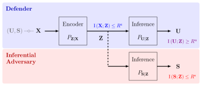
Figure 3: The CLUB model.

3.3 Problem Formulation

Given three dependent (correlated) random variables $\mathbf{U}$, $\mathbf{S}$ and $\mathbf{X}$ with joint distribution $P_{\mathbf{U,S,X}}\,$, the goal of the CLUB model is to find a representation $\mathbf{Z}$ of $\mathbf{X}$ using a stochastic mapping $P_{\mathbf{Z}\mid\mathbf{X}}$ such that: (i) $\left(\mathbf{U},\mathbf{S}\right)\hbox{$\--$}\kern-1.5pt\hbox{$\circ$}\kern-1.5pt\hbox{$\--$}\mathbf{X}\hbox{$\--$}\kern-1.5pt\hbox{$\circ$}\kern-1.5pt\hbox{$\--$}\mathbf{Z}$, and (ii) representation $\mathbf{Z}$ is maximally informative about $\mathbf{U}$ (maximizing $\mathrm{I}\left(\mathbf{U};\mathbf{Z}\right)$) while being minimally informative about $\mathbf{X}$ (minimizing $\mathrm{I}\left(\mathbf{X};\mathbf{Z}\right)$) and minimally informative about $\mathbf{S}$ (minimizing $\mathrm{I}\left(\mathbf{S};\mathbf{Z}\right)$). We can formulate this three-dimensional trade-off by imposing constraints on the two of them. That is, for a given information complexity and information leakage constraints, $R^{\mathrm{z}}\geq 0$ and $R^{\mathrm{s}}\geq 0$, respectively, this trade-off can be formulated by a CLUB functional:

$$\mathsf{CLUB}\left(R^{\mathrm{z}},R^{\mathrm{s}},P_{\mathbf{U},\mathbf{S},\mathbf{X}}\right)\coloneqq\mathop{\sup}_{\begin{subarray}{c}P_{\mathbf{Z}\mid\mathbf{X}}:\\ \left(\mathbf{U},\mathbf{S}\right)\hbox{$\--$}\kern-1.5pt\hbox{$\circ$}\kern-1.5pt\hbox{$\--$}\mathbf{X}\hbox{$\--$}\kern-1.5pt\hbox{$\circ$}\kern-1.5pt\hbox{$\--$}\mathbf{Z}\end{subarray}}\mathrm{I}\left(\mathbf{U};\mathbf{Z}\right)\;\quad\;\mathrm{s.t.}\quad\mathrm{I}\left(\mathbf{X};\mathbf{Z}\right)\leq R^{\mathrm{z}},\;\;\mathrm{I}\left(\mathbf{S};\mathbf{Z}\right)\leq R^{\mathrm{s}}.$$ (7)

The constraint $\mathrm{I}\left(\mathbf{S};\mathbf{Z}\right)\leq R^{\mathrm{s}}$ ensures that $\mathrm{H}\left(\mathbf{S}\mid\mathbf{Z}\right)\geq\mathrm{H}\left(\mathbf{S}\right)-R^{\mathrm{s}}=E^{\mathrm{a}}$, where $E^{\mathrm{a}}$ quantifies the amount of uncertainty for adversary. On the other hand, note that $\mathrm{I}\left(\mathbf{S};\mathbf{Z}\right)=\mathbb{E}_{P_{\mathbf{Z}}}\left[\mathrm{D}_{\mathrm{KL}}\left(P_{\mathbf{S}\mid\mathbf{Z}}\|P_{\mathbf{S}}\right)\right]$. This means that for small values of $R^{\mathrm{s}}$, the posterior of private attribute $\mathbf{S}$ given released representation $\mathbf{Z}$, i.e., $P_{\mathbf{S}\mid\mathbf{Z}}$, is as close as possible to the prior $P_{\mathbf{S}}$. The constraint $\mathrm{I}\left(\mathbf{X};\mathbf{Z}\right)\leq R^{\mathrm{z}}$ controls information complexity (aka compactness) of representations and goes beyond a simple regularization term. Indeed, it is related to the notion of encoder capacity [79, 80], which is a measure of distinguishability among input data samples from their released representations. Moreover, the information complexity $\mathrm{I}\left(\mathbf{X};\mathbf{Z}\right)$ establishes a fundamental relation to the generalization capability of the stochastic encoder model $P_{\mathbf{Z}\mid\mathbf{X}}$. The trade-off in (7) was studied in [51], where the constraint on $\mathrm{I}\left(\mathbf{U};\mathbf{Z}\right)$ is motivated as a rate-constraint, and the trade-off is studied under perfect privacy regime (i.e., $\mathrm{I}\left(\mathbf{S};\mathbf{Z}\right)=0$). Note that by controlling the rate $R^{\mathrm{z}}$, the defender (data owner) exploits the imposed distortion at the utility service provider (authorized decoder) to control the uncertainty for the adversary (non-authorized decoder). The values $\mathsf{CLUB}\left(R^{\mathrm{z}},R^{\mathrm{s}},P_{\mathbf{U},\mathbf{S},\mathbf{X}}\right)$ for different $R^{\mathrm{z}}$ and $R^{\mathrm{s}}$ specify the CLUB curve.

Alternatively, one may impose constraints on useful information $\mathrm{I}\left(\mathbf{U};\mathbf{Z}\right)$ and disclosed private information $\mathrm{I}\left(\mathbf{S};\mathbf{Z}\right)$, which leads to:

$$\mathsf{CLUB}\left(R^{\mathrm{u}},R^{\mathrm{s}},P_{\mathbf{U},\mathbf{S},\mathbf{X}}\right)\coloneqq\mathop{\inf}_{\begin{subarray}{c}P_{\mathbf{Z}\mid\mathbf{X}}:\\ \left(\mathbf{U},\mathbf{S}\right)\hbox{$\--$}\kern-1.5pt\hbox{$\circ$}\kern-1.5pt\hbox{$\--$}\mathbf{X}\hbox{$\--$}\kern-1.5pt\hbox{$\circ$}\kern-1.5pt\hbox{$\--$}\mathbf{Z}\end{subarray}}\mathrm{I}\left(\mathbf{X};\mathbf{Z}\right)\;\quad\;\mathrm{s.t.}\quad\mathrm{I}\left(\mathbf{U};\mathbf{Z}\right)\geq R^{\mathrm{u}},\;\;\mathrm{I}\left(\mathbf{S};\mathbf{Z}\right)\leq R^{\mathrm{s}}.$$ (8)

In order to explore the CLUB curve, one must find the optimal bottleneck representation $\mathbf{Z}$ for different values of $R^{\mathrm{z}}$ and $R^{\mathrm{s}}$ ($R^{\mathrm{u}}$ and $R^{\mathrm{s}}$). In practice, the CLUB curve is explored by maximizing (minimizing) its associated Lagrangian functional. Therefore, equivalently, with the introduction of a Lagrange multipliers $\beta,\alpha\in\left[0,1\right]$ and $\gamma,\lambda\in\left(0,+\infty\right)$, we can formulate the CLUB problem by the associated Lagrangian functional. In particular, the two associated CLUB Lagrangian functionals of our interest are given as follows:

$$\mathcal{L}_{\mathrm{CLUB}}\left(P_{\mathbf{Z}\mid\mathbf{X}},\beta,\alpha\right) \coloneqq\mathrm{I}\left(\mathbf{U};\mathbf{Z}\right)-\beta\,\mathrm{I}\left(\mathbf{X};\mathbf{Z}\right)-\alpha\,\mathrm{I}\left(\mathbf{S};\mathbf{Z}\right),$$ (9a)

$$\mathcal{L}_{\mathrm{CLUB}}\left(P_{\mathbf{Z}\mid\mathbf{X}},\gamma,\lambda\right) \coloneqq\mathrm{I}\left(\mathbf{X};\mathbf{Z}\right)-\gamma\,\mathrm{I}\left(\mathbf{U};\mathbf{Z}\right)+\lambda\,\mathrm{I}\left(\mathbf{S};\mathbf{Z}\right).$$ (9b)

Consider the set of 3-dimensional mutual information region for $\left(\mathbf{U},\mathbf{S},\mathbf{X}\right)\sim P_{\mathbf{U},\mathbf{S},\mathbf{X}}$, defined as follows:

$$\mathcal{I}\left(P_{\mathbf{U},\mathbf{S},\mathbf{X}}\right)\coloneqq\bigcup_{P_{\mathbf{Z}\mid\mathbf{X}}}\Big{\{}\mathrm{I}\left(\mathbf{U};\mathbf{Z}\right),\mathrm{I}\left(\mathbf{S};\mathbf{Z}\right),\mathrm{I}\left(\mathbf{X};\mathbf{Z}\right):\left(\mathbf{U},\mathbf{S}\right)\hbox{$\--$}\kern-1.5pt\hbox{$\circ$}\kern-1.5pt\hbox{$\--$}\mathbf{X}\hbox{$\--$}\kern-1.5pt\hbox{$\circ$}\kern-1.5pt\hbox{$\--$}\mathbf{Z}\Big{\}}\subseteq\mathbb{R}^{3}.$$ (10)

Also, consider the constrained information regions $\mathcal{R}\left(P_{\mathbf{U},\mathbf{S},\mathbf{X}}\right)$, defined as follows:

$$\mathcal{R}\left(P_{\mathbf{U},\mathbf{S},\mathbf{X}}\right)\coloneqq\big{\{}\left(R^{\mathrm{u}},R^{\mathrm{s}},R^{\mathrm{z}}\right)\in\mathcal{I}_{\mathbf{U},\mathbf{S},\mathbf{X}}:\;\mathrm{I}\left(\mathbf{U};\mathbf{Z}\right)\geq R^{\mathrm{u}},\mathrm{I}\left(\mathbf{S};\mathbf{Z}\right)\leq R^{\mathrm{s}},\mathrm{I}\left(\mathbf{X};\mathbf{Z}\right)\leq R^{\mathrm{z}}\big{\}}.$$ (11)

In Sec. 6.1, we show that the CLUB model subsumes most previously reported information-theoretic privacy models. More specifically, we show that the mutual information region $\mathcal{I}\left(P_{\mathbf{U},\mathbf{S},\mathbf{X}}\right)$ subsumes the recent models proposed in [62, 81, 82].

4 Variational CLUB

Direct optimization of (9a) to obtain the optimal stochastic mapping $P_{\mathbf{Z}\mid\mathbf{X}}$ is generally challenging. Instead, a tight variational bound can be optimized. Let $Q_{\mathbf{U}\mid\mathbf{Z}}:\mathcal{Z}\rightarrow\mathcal{P}\left(\mathcal{U}\right)$, $Q_{\mathbf{X}\mid\mathbf{S},\mathbf{Z}}:\mathcal{S}\times\mathcal{Z}\rightarrow\mathcal{P}\left(\mathcal{X}\right)$ and $Q_{\mathbf{Z}}:\mathcal{Z}\rightarrow\mathcal{P}\left(\mathcal{Z}\right)$ be variational approximations of the optimal utility decoder distribution $P_{\mathbf{U}\mid\mathbf{Z}}$, uncertainty decoder distribution $P_{\mathbf{X}\mid\mathbf{S},\mathbf{Z}}$, and latent space distribution $P_{\mathbf{Z}}$, respectively. In the sequel, we will obtain a variational bound $\mathcal{L}_{\mathrm{VCLUB}}\left(P_{\mathbf{Z}\mid\mathbf{X}},Q_{\mathbf{U}\mid\mathbf{Z}},Q_{\mathbf{Z}},Q_{\mathbf{X}\mid\mathbf{S},\mathbf{Z}},\beta,\alpha\right)$, such that for any valid mapping $P_{\mathbf{Z}\mid\mathbf{X}}$ satisfying the Markov chain condition $\left(\mathbf{U},\mathbf{S}\right)\hbox{$\--$}\kern-1.5pt\hbox{$\circ$}\kern-1.5pt\hbox{$\--$}\mathbf{X}\hbox{$\--$}\kern-1.5pt\hbox{$\circ$}\kern-1.5pt\hbox{$\--$}\mathbf{Z}$, we have:

$$\mathcal{L}_{\mathrm{CLUB}}\left(P_{\mathbf{Z}\mid\mathbf{X}},\beta,\alpha\right)\geq\mathcal{L}_{\mathrm{VCLUB}}\left(P_{\mathbf{Z}\mid\mathbf{X}},Q_{\mathbf{U}\mid\mathbf{Z}},Q_{\mathbf{Z}},Q_{\mathbf{X}\mid\mathbf{S},\mathbf{Z}},\beta,\alpha\right).$$ (12)

The inequality holds with equality, if the variational approximations match the true distributions, i.e., when $Q_{\mathbf{U}\mid\mathbf{Z}}=P_{\mathbf{U}\mid\mathbf{Z}}$, $Q_{\mathbf{X}\mid\mathbf{S},\mathbf{Z}}=P_{\mathbf{X}\mid\mathbf{S},\mathbf{Z}}$, and $Q_{\mathbf{Z}}=P_{\mathbf{Z}}$. Since (12) holds for any $P_{\mathbf{Z}\mid\mathbf{X}}$, instead of maximizing $\mathcal{L}_{\mathrm{CLUB}}\left(P_{\mathbf{Z}\mid\mathbf{X}},\beta,\alpha\right)$, we will maximize $\mathcal{L}_{\mathrm{VCLUB}}\left(P_{\mathbf{Z}\mid\mathbf{X}},Q_{\mathbf{U}\mid\mathbf{Z}},Q_{\mathbf{Z}},Q_{\mathbf{X}\mid\mathbf{S},\mathbf{Z}},\beta,\alpha\right)$ over the variational distributions.

Alternatively, consider the CLUB Lagrangian functional (9b) and let $\mathcal{L}_{\mathrm{VCLUB}}\left(P_{\mathbf{Z}\mid\mathbf{X}},Q_{\mathbf{U}\mid\mathbf{Z}},Q_{\mathbf{Z}},Q_{\mathbf{X}\mid\mathbf{S},\mathbf{Z}},\gamma,\lambda\right)$ be the obtained variational bound. For any valid mapping $P_{\mathbf{Z}\mid\mathbf{X}}$ satisfying the Markov chain condition $\left(\mathbf{U},\mathbf{S}\right)\hbox{$\--$}\kern-1.5pt\hbox{$\circ$}\kern-1.5pt\hbox{$\--$}\mathbf{X}\hbox{$\--$}\kern-1.5pt\hbox{$\circ$}\kern-1.5pt\hbox{$\--$}\mathbf{Z}$, we have:

$$\mathcal{L}_{\mathrm{CLUB}}\left(P_{\mathbf{Z}\mid\mathbf{X}},\gamma,\lambda\right)\leq\mathcal{L}_{\mathrm{VCLUB}}\left(P_{\mathbf{Z}\mid\mathbf{X}},Q_{\mathbf{U}\mid\mathbf{Z}},Q_{\mathbf{Z}},Q_{\mathbf{X}\mid\mathbf{S},\mathbf{Z}},\gamma,\lambda\right).$$ (13)

4.1 Variational Bound on Information Complexity

The information complexity $\mathrm{I}\left(\mathbf{X};\mathbf{Z}\right)$ can be decomposed as:

$$\mathrm{I}\left(\mathbf{X};\mathbf{Z}\right)=\mathbb{E}_{P_{\mathbf{X},\mathbf{Z}}}\left[\log\frac{P_{\mathbf{X},\mathbf{Z}}}{P_{\mathbf{X}}P_{\mathbf{Z}}}\right]=\mathbb{E}_{P_{\mathbf{X},\mathbf{Z}}}\left[\log\frac{P_{\mathbf{Z}\mid\mathbf{X}}}{P_{\mathbf{Z}}}\right] = \mathbb{E}_{P_{\mathbf{X},\mathbf{Z}}}\left[\log\frac{P_{\mathbf{Z}\mid\mathbf{X}}}{Q_{\mathbf{Z}}}\right]-\mathrm{D}_{\mathrm{KL}}\left(P_{\mathbf{Z}}\|Q_{\mathbf{Z}}\right)$$ (14)

$$= \mathrm{D}_{\mathrm{KL}}\left(P_{\mathbf{Z}\mid\mathbf{X}}\|Q_{\mathbf{Z}}\mid P_{\mathbf{X}}\right)-\mathrm{D}_{\mathrm{KL}}\left(P_{\mathbf{Z}}\|Q_{\mathbf{Z}}\right),$$ (15)

where $\mathrm{D}_{\mathrm{KL}}\left(P_{\mathbf{Z}\mid\mathbf{X}}\|Q_{\mathbf{Z}}\mid P_{\mathbf{X}}\right)$ is the conditional divergence. Since $\mathrm{D}_{\mathrm{KL}}\left(P_{\mathbf{Z}}\|Q_{\mathbf{Z}}\right)\geq 0$, we can upper bound (14) as:

$$\mathrm{I}\left(\mathbf{X};\mathbf{Z}\right)\leq\mathrm{D}_{\mathrm{KL}}\left(P_{\mathbf{Z}\mid\mathbf{X}}\|Q_{\mathbf{Z}}\mid P_{\mathbf{X}}\right).$$ (16)

Hence, one can minimize the information complexity upper bound (16), instead of minimizing (14). Note that the information complexity is completely characterized using two terms $\mathrm{D}_{\mathrm{KL}}\left(P_{\mathbf{Z}\mid\mathbf{X}}\|Q_{\mathbf{Z}}\mid P_{\mathbf{X}}\right)$ and $\mathrm{D}_{\mathrm{KL}}\left(P_{\mathbf{Z}}\|Q_{\mathbf{Z}}\right)$.

4.2 Variational Bound on Information Utility

We can decompose the mutual information between the released representation $\mathbf{Z}$ and the utility attribute $\mathbf{U}$ in two analytically equivalent ways:

$$\mathrm{I}\left(\mathbf{U};\mathbf{Z}\right)=\underbrace{\mathrm{H}\left(\mathbf{U}\right)-\mathrm{H}\left(\mathbf{U}\mid\mathbf{Z}\right)}_{\mathrm{Discriminative~{}View}}=\underbrace{\mathrm{H}\left(\mathbf{Z}\right)-\mathrm{H}\left(\mathbf{Z}\mid\mathbf{U}\right)}_{\mathrm{Generative~{}View}}.$$ (17)

Therefore, maximizing $\mathrm{I}\left(\mathbf{U};\mathbf{Z}\right)$ can have two different interpretations. The discriminative view expresses that (i) the utility attribute needs to be distributed as uniformly as possible in the data space, and (ii) the utility attribute should be confidently inferred from the released representation $\mathbf{Z}$. On the other hand, the generative view expresses that (i) the released representations should be spread as much as possible in the latent space (i.e., high entropy $\mathrm{H}(\mathbf{Z})$), and (ii) the released representation corresponding to the same utility attribute should be close together (i.e., minimizing conditional entropy $\mathrm{H}(\mathbf{Z}\!\mid\!\mathbf{U})$). Since our goal is to identify the utility attributes based on the revealed representation, the discriminative view of this decomposition is more aligned with our model. We rewrite the conditional entropy term as follows:

$$\mathrm{H}\left(\mathbf{U}\mid\mathbf{Z}\right) =\mathbb{E}_{P_{\mathbf{U},\mathbf{Z}}}\left[\log P_{\mathbf{U}\mid\mathbf{Z}}\right]$$ (18a)

$$=\mathbb{E}_{P_{\mathbf{U},\mathbf{Z}}}\left[\log Q_{\mathbf{U}\mid\mathbf{Z}}\right]+\mathbb{E}_{P_{\mathbf{U},\mathbf{Z}}}\left[\log\frac{P_{\mathbf{U}\mid\mathbf{Z}}}{Q_{\mathbf{U}\mid\mathbf{Z}}}\right]$$ (18b)

$$=\mathbb{E}_{P_{\mathbf{U},\mathbf{Z}}}\left[\log Q_{\mathbf{U}\mid\mathbf{Z}}\right]+\mathrm{D}_{\mathrm{KL}}\left(P_{\mathbf{U}\mid\mathbf{Z}}\|Q_{\mathbf{U}\mid\mathbf{Z}}\mid P_{\mathbf{Z}}\right).$$ (18c)

Note that $\mathrm{H}\left(P_{\mathbf{U}\mid\mathbf{Z}}\|Q_{\mathbf{U}\mid\mathbf{Z}}\mid P_{\mathbf{Z}}\right)\coloneqq\mathbb{E}_{P_{\mathbf{Z}}}\left[\mathbb{E}_{P_{\mathbf{U}\mid\mathbf{Z}}}\left[\log Q_{\mathbf{U}\mid\mathbf{Z}}\right]\right]=\mathbb{E}_{P_{\mathbf{U},\mathbf{Z}}}\left[\log Q_{\mathbf{U}\mid\mathbf{Z}}\right]$ is the cross-entropy loss function. Since $\mathrm{D}_{\mathrm{KL}}\left(P_{\mathbf{U}\mid\mathbf{Z}}\|Q_{\mathbf{U}\mid\mathbf{Z}}\mid P_{\mathbf{Z}}\right)\geq 0$, we can lower bound information utility as:

$$\mathrm{I}\left(\mathbf{U};\mathbf{Z}\right)\geq\mathrm{H}\left(\mathbf{U}\right)-\mathrm{H}\left(P_{\mathbf{U}\mid\mathbf{Z}}\|Q_{\mathbf{U}\mid\mathbf{Z}}\mid P_{\mathbf{Z}}\right).$$ (19)

According to (19), the minimization of the average cross-entropy loss leads to the maximization of (a lower bound of) the information gain $\mathrm{I}\left(\mathbf{U};\mathbf{Z}\right)$. Therefore, if the conditional distributions are very close to each other, i.e., if the gap $\mathrm{D}_{\mathrm{KL}}\left(P_{\mathbf{U}\mid\mathbf{Z}}\|Q_{\mathbf{U}\mid\mathbf{Z}}\mid P_{\mathbf{Z}}\right)$ is small, by minimizing the average cross-entropy loss $\mathrm{H}\left(P_{\mathbf{U}\mid\mathbf{Z}}\|Q_{\mathbf{U}\mid\mathbf{Z}}\mid P_{\mathbf{Z}}\right)$ over representations, we can achieve a tight upper bound on the decoder’s uncertainty $\mathrm{H}\left(\mathbf{U}\!\mid\!\mathbf{Z}\right)$. Furthermore, note that minimizing $\mathrm{H}\left(\mathbf{U}\!\mid\!\mathbf{Z}\right)$ leads to a small probability of error in the prediction of the (discrete) utility attribute from released representation.

Remark 3 (From supervised CLUB to unsupervised CLUB).

Let us consider a scenario in which the data owner wishes to release the original domain data $\mathbf{X}$ (e.g., facial images) as accurately as possible (i.e., $\mathbf{U}\equiv\mathbf{X}$), without revealing a specific sensitive attribute $\mathbf{S}$ (e.g., gender, emotion, etc.). We call this setup as the unsupervised CLUB model and the formerly described general case, where $\mathbf{U}$ is a generic attribute of data $\mathbf{X}$ as the supervised CLUB model. In the unsupervised scenario, we can proceed with a similar decomposition as derived above, but with a few modifications. For the sake of brevity, we address this decomposition in Sec. 5, after introducing our parameterized variational approximation of the distributions.

4.3 Variational Bound on Information Leakage

One can obtain a variational lower bound on $\mathrm{I}\left(\mathbf{S};\mathbf{Z}\right)$ similarly to the one obtained in (19), that is:

$$\mathrm{I}\left(\mathbf{S};\mathbf{Z}\right)\geq\mathrm{H}\left(\mathbf{S}\right)+\mathbb{E}_{P_{\mathbf{S},\mathbf{X}}}\left[\mathbb{E}_{P_{\mathbf{Z}\mid\mathbf{X}}}\left[\log Q_{\mathbf{S}\mid\mathbf{Z}}\right]\right].$$ (20)

However, we want to minimize $\mathrm{I}\left(\mathbf{S};\mathbf{Z}\right)$; therefore, we instead need a variational upper bound. Alternatively, we can express $\mathrm{I}\left(\mathbf{S};\mathbf{Z}\right)$ as:

$$\mathrm{I}\left(\mathbf{S};\mathbf{Z}\right) = \mathrm{I}\left(\mathbf{X};\mathbf{Z}\right)-\mathrm{I}\left(\mathbf{X};\mathbf{Z}\mid\mathbf{S}\right)$$ (21)

$$= \mathrm{I}\left(\mathbf{X};\mathbf{Z}\right)-\mathrm{H}\left(\mathbf{X}\mid\mathbf{S}\right)+\mathrm{H}\left(\mathbf{X}\mid\mathbf{S},\mathbf{Z}\right).$$

By utilizing the variational approximation $Q_{\mathbf{X}\mid\mathbf{S},\mathbf{Z}}$ for the conditional entropy $\mathrm{H}\left(\mathbf{X}\!\mid\!\mathbf{S},\mathbf{Z}\right)$, we have:

$$\mathrm{H}\left(\mathbf{X}\!\mid\!\mathbf{S},\mathbf{Z}\right)=-\mathbb{E}_{P_{\mathbf{S},\mathbf{X},\mathbf{Z}}}\left[\log P_{\mathbf{X}\mid\mathbf{S},\mathbf{Z}}\right]=-\mathbb{E}_{P_{\mathbf{S},\mathbf{X}}}\left[\mathbb{E}_{P_{\mathbf{Z}\mid\mathbf{X}}}\left[\log Q_{\mathbf{X}\mid\mathbf{S},\mathbf{Z}}\right]\right]-\mathrm{D}_{\mathrm{KL}}\left(P_{\mathbf{X}\mid\mathbf{S},\mathbf{Z}}\|Q_{\mathbf{X}\mid\mathbf{S},\mathbf{Z}}\right).\vspace{-4pt}$$ (22)

Considering $\mathrm{D}_{\mathrm{KL}}\left(P_{\mathbf{X}\mid\mathbf{S},\mathbf{Z}}\|Q_{\mathbf{X}\mid\mathbf{S},\mathbf{Z}}\right)\geq 0$ and using (16), we can obtain an upper bound on $\mathrm{I}\left(\mathbf{S};\mathbf{Z}\right)$ as:

$$\mathrm{I}\left(\mathbf{S};\mathbf{Z}\right)\leq\mathrm{D}_{\mathrm{KL}}\left(P_{\mathbf{Z}\mid\mathbf{X}}\|Q_{\mathbf{Z}}\mid P_{\mathbf{X}}\right)+\mathrm{H}\left(\mathbf{X}\mid\mathbf{S}\right)+\mathrm{H}\left(P_{\mathbf{X}\mid\mathbf{S,Z}}\|Q_{\mathbf{X}\mid\mathbf{S,Z}}\mid P_{\mathbf{S,Z}}\right),\vspace{-4pt}$$ (23)

where $\mathrm{H}\left(P_{\mathbf{X}\mid\mathbf{S,Z}}\|Q_{\mathbf{X}\mid\mathbf{S,Z}}\mid P_{\mathbf{S,Z}}\right)\coloneqq\mathbb{E}_{P_{\mathbf{S},\mathbf{X},\mathbf{Z}}}\left[\log Q_{\mathbf{X}\mid\mathbf{S},\mathbf{Z}}\right]$. Eqn. (21) depicts the critical role of information complexity $\mathrm{I}\left(\mathbf{X};\mathbf{Z}\right)$ in controlling the information leakage $\mathrm{I}\left(\mathbf{S};\mathbf{Z}\right)$. The less the information complexity, the less distinguishable the revealed representations, and hence the less the information leakage. The term $\mathrm{H}\!\left(P_{\mathbf{X}\mid\mathbf{S,Z}}\|Q_{\mathbf{X}\mid\mathbf{S,Z}}\!\mid\!P_{\mathbf{S,Z}}\right)$ can be interpreted as follows. Consider the inference threat model presented in Sec. 2.2. The inferential adversary has access to the revealed representation $\mathbf{Z}$ and is interested in inferring the sensitive attribute $\mathbf{S}$. Note that the adversary’s inference is through reconstructing the original data $\mathbf{X}$. Therefore, after observing $\mathbf{Z}$, the adversary chooses a belief distribution over $\mathcal{S}$ and then tries to reconstruct the original data $\mathbf{X}$ to revise his belief. If the released representation is statistically independent of the sensitive attribute $\mathbf{S}$, then the adversary cannot revise his belief by injecting various $\mathbf{S}$ to his inferential model. Hence, by maximizing the average log-likelihood $\log Q_{\mathbf{X}\mid\mathbf{S},\mathbf{Z}}$ over $P_{\mathbf{Z}\mid\mathbf{X}}$, the defender minimizes the average adversarial inference about $\mathbf{S}$.

Considering (16), (19), and (23), in the supervised scenario, the VCLUB bound in (12) can be written as:

$$\mathcal{L}_{\mathrm{VCLUB}}^{\mathsf{S}}\left(P_{\mathbf{Z}\mid\mathbf{X}},Q_{\mathbf{U}\mid\mathbf{Z}},Q_{\mathbf{Z}},Q_{\mathbf{X}\mid\mathbf{S},\mathbf{Z}},\beta,\alpha\right)$$

$$=\mathbb{E}_{P_{\mathbf{U},\mathbf{X}}}\left[\mathbb{E}_{P_{\mathbf{Z}\mid\mathbf{X}}}\left[\log Q_{\mathbf{U}\mid\mathbf{Z}}\right]\right]-\left(\beta+\alpha\right)\mathbb{E}_{P_{\mathbf{X},\mathbf{Z}}}\left[\log\frac{P_{\mathbf{Z}\mid\mathbf{X}}}{Q_{\mathbf{Z}}}\right]+\alpha\,\mathbb{E}_{P_{\mathbf{S},\mathbf{X}}}\left[\mathbb{E}_{P_{\mathbf{Z}\mid\mathbf{X}}}\left[\log Q_{\mathbf{X}\mid\mathbf{S},\mathbf{Z}}\right]\right]+\mathrm{c},\vspace{-4pt}$$ (24)

where $\mathrm{c}$ is a constant term. For the sake of brevity, we directly address the unsupervised DVCLUB in Sec. 5.

5 Deep Variational CLUB (DVCLUB)

The common approach is to use neural networks to parameterize variational inference bounds. To this goal, we parameterize the encoding distribution $P_{\mathbf{Z}\mid\mathbf{X}}$, utility decoding distribution $Q_{\mathbf{U}\mid\mathbf{Z}}$, uncertainty decoding distribution $Q_{\mathbf{X}\mid\mathbf{S,Z}}$, and prior $Q_{\mathbf{Z}}$. Let $P_{\bm{\phi}}(\mathbf{Z}\!\mid\!\mathbf{X})$ denote the family of encoding probability distributions $P_{\mathbf{Z}\mid\mathbf{X}}$ over $\mathcal{Z}$ for each element of space $\mathcal{X}$, parameterized by the output of a deep neural network $f_{\bm{\phi}}$ with parameters $\bm{\phi}$. In the context of inference problems, $P_{\bm{\phi}}(\mathbf{Z}\!\mid\!\mathbf{X})$ is called the amortized variational inference (AVI) distribution or variational posterior distribution. Analogously, let $P_{\bm{\theta}}(\mathbf{U}\!\mid\!\mathbf{Z})$ and $P_{\bm{\varphi}}\!\left(\mathbf{X}\!\mid\!\mathbf{S},\mathbf{Z}\right)$ denote the corresponding family of decoding probability distributions $Q_{\mathbf{U}\mid\mathbf{Z}}$ and $Q_{\mathbf{X}\mid\mathbf{S},\mathbf{Z}}$, respectively, parameterized by the output of the deep neural networks $g_{\bm{\theta}}$ and $g_{\bm{\varphi}}$. Moreover, for the prior distribution $Q_{\mathbf{Z}}$ we consider the family of distributions $Q_{\bm{\psi}}\!\left(\mathbf{Z}\right)$, which can be interpreted as the target (proposal) distribution in the latent space. The choice for these distributions is considered by trading off computational complexity with model expressiveness. Let $P_{\mathsf{D}}\!\left(\mathbf{X}\right)\!=\!\!\frac{1}{N}\!\sum_{n=1}^{N}\!\delta(\mathbf{x}-\mathbf{x}_{n})$, $\mathbf{x}_{n}\!\!\in\!\mathcal{X}$, denote the empirical data distribution. In this case, $P_{\!\bm{\phi}}\!\left(\mathbf{X},\mathbf{Z}\right)\!=\!P_{\mathsf{D}}(\mathbf{X})P_{\!\bm{\phi}}\!\left(\mathbf{Z}\!\mid\!\mathbf{X}\right)$ denotes our joint inference data distribution, and $P_{\!\bm{\phi}}(\mathbf{Z})\!=\!\mathbb{E}_{\!P_{\mathsf{D}}(\mathbf{X})}\!\left[P_{\!\bm{\phi}}(\mathbf{Z}\!\mid\!\mathbf{X})\right]$ denotes the learned aggregated posterior distribution over latent space $\mathcal{Z}$.

Parameterized Information Complexity: The parameterized variational approximation of information complexity (14) can be defined as:

$$\mathrm{I}_{\bm{\phi},\bm{\psi}}\!\left(\mathbf{X};\mathbf{Z}\right)\coloneqq\mathrm{D}_{\mathrm{KL}}\!\left(P_{\bm{\phi}}(\mathbf{Z}\!\mid\!\mathbf{X})\,\|\,Q_{\bm{\psi}}(\mathbf{Z})\mid P_{\mathsf{D}}(\mathbf{X})\right)-\mathrm{D}_{\mathrm{KL}}\!\left(P_{\bm{\phi}}(\mathbf{Z})\,\|\,Q_{\bm{\psi}}(\mathbf{Z})\right).$$ (25)

Indeed, the information complexity $\mathrm{I}_{\bm{\phi},\bm{\psi}}\!\left(\mathbf{X};\mathbf{Z}\right)$ measures the amount of Shannon’s mutual information between the parameters of the model and the dataset $\mathsf{D}$, given a prior $Q_{\bm{\psi}}(\mathbf{Z})$ and stochastic map $P_{\bm{\phi}}(\mathbf{Z}\!\mid\!\mathbf{X}):\mathcal{X}\rightarrow\mathcal{P}(\mathcal{Z})$. Note that the posterior distribution $P_{\bm{\phi}}(\mathbf{Z}\!\mid\!\mathbf{X})$ depends on the choice of the optimization algorithm, therefore, the information complexity implicitly depends on this choice. The relative entropy $\mathrm{D}_{\mathrm{KL}}\!\left(P_{\bm{\phi}}(\mathbf{Z})\,\|\,Q_{\bm{\psi}}(\mathbf{Z})\right)$ is usually ignored in the literature. A critical challenge is to guarantee that the learned aggregated posterior distribution $P_{\bm{\phi}}(\mathbf{Z})$ conforms well to the proposed prior $Q_{\bm{\psi}}\!\left(\mathbf{Z}\right)$ [83, 84, 85, 86, 87]. We can tackle this issue by employing a more expressive form for $Q_{\bm{\psi}}\!\left(\mathbf{Z}\right)$, which would allow us to provide a good fit for an arbitrary space $\mathcal{Z}$, at the expense of additional computational complexity.

From (25), we have:

$$\!\!\!\!\!\!\mathrm{I}_{\bm{\phi},\bm{\psi}}\!\left(\mathbf{X};\mathbf{Z}\right) \leq\mathrm{D}_{\mathrm{KL}}\!\left(P_{\bm{\phi}}(\mathbf{Z}\!\mid\!\mathbf{X})\,\|\,Q_{\bm{\psi}}(\mathbf{Z})\mid P_{\mathsf{D}}(\mathbf{X})\right)$$ (26a)

$$=\mathbb{E}_{P_{\mathsf{D}}(\mathbf{X})}\Big{[}\mathbb{E}_{P_{\bm{\phi}}(\mathbf{Z}\mid\mathbf{X})}\Big{[}\log\frac{P_{\bm{\phi}}(\mathbf{Z}\!\mid\!\mathbf{X})}{Q_{\bm{\psi}}(\mathbf{Z})}\Big{]}\Big{]}$$ (26b)

$$=\mathbb{E}_{P_{\mathsf{D}}(\mathbf{X})}\left[\mathbb{E}_{P_{\bm{\phi}}(\mathbf{Z}\mid\mathbf{X})}\big{[}\log P_{\bm{\phi}}(\mathbf{Z}\!\mid\!\mathbf{X})\big{]}\right]-\mathbb{E}_{P_{\bm{\phi}}(\mathbf{Z})}\left[\log Q_{\bm{\psi}}(\mathbf{Z})\right]$$ (26c)

$$=-\mathbb{E}_{P_{\mathsf{D}}(\mathbf{X})}\left[\,\mathrm{H}\left(P_{\bm{\phi}}(\mathbf{Z}\!\mid\!\mathbf{X}=\mathbf{x})\right)\,\right]+\mathrm{H}\left(P_{\bm{\phi}}(\mathbf{Z})\|Q_{\bm{\psi}}(\mathbf{Z})\right).$$ (26d)

Therefore, if $\mathrm{D}_{\mathrm{KL}}\!\left(P_{\bm{\phi}}(\mathbf{Z})\,\|\,Q_{\bm{\psi}}(\mathbf{Z})\right)$ is small, minimizing the cross-entropy term $\mathrm{H}\left(P_{\bm{\phi}}(\mathbf{Z})\|Q_{\bm{\psi}}(\mathbf{Z})\right)$ provides an upper bound on the information complexity. Note that by imposing a constraint on the information complexity $\mathrm{I}_{\bm{\phi},\bm{\psi}}\!\left(\mathbf{X};\mathbf{Z}\right)$, we are imposing a constraint on the entropy of the AVI distribution $P_{\bm{\phi}}(\mathbf{Z})$.

Parameterized Information Utility: The parameterized variational approximation associated to the information utility bound in (19) can be defined as:

$$\mathrm{I}_{\bm{\phi},\bm{\theta}}\!\left(\mathbf{U};\mathbf{Z}\right) \coloneqq\mathrm{H}(\mathbf{U})-\mathrm{H}\left(P_{\mathbf{U}\mid\mathbf{Z}}\,\|\,P_{\bm{\theta}}\!\left(\mathbf{U}\!\mid\!\mathbf{Z}\right)\mid P_{\bm{\phi}}(\mathbf{Z})\right)+\mathrm{D}_{\mathrm{KL}}\left(P_{\mathbf{U}\mid\mathbf{Z}}\,\|\,P_{\bm{\theta}}\!\left(\mathbf{U}\!\mid\!\mathbf{Z}\right)\mid P_{\bm{\phi}}(\mathbf{Z})\right)$$ (27a)

$$\geq\mathrm{H}(\mathbf{U})-\mathrm{H}\left(P_{\mathbf{U}\mid\mathbf{Z}}\,\|\,P_{\bm{\theta}}\!\left(\mathbf{U}\!\mid\!\mathbf{Z}\right)\mid P_{\bm{\phi}}(\mathbf{Z})\right)=\mathrm{H}(\mathbf{U})-\mathrm{H}_{\bm{\phi},\bm{\theta}}\left(\mathbf{U}\!\mid\!\mathbf{Z}\right),$$ (27b)

where $\mathrm{H}_{\bm{\phi},\bm{\theta}}\left(\mathbf{U}\!\mid\!\mathbf{Z}\right)\coloneqq\mathrm{H}\left(P_{\mathbf{U}\mid\mathbf{Z}}\,\|\,P_{\bm{\theta}}\!\left(\mathbf{U}\!\mid\!\mathbf{Z}\right)\mid P_{\bm{\phi}}(\mathbf{Z})\right)$.

Alternatively, we can decompose $\mathrm{I}_{\bm{\phi},\bm{\theta}}\!\left(\mathbf{U};\mathbf{Z}\right)$ as follows:

$$\mathrm{I}_{\bm{\phi},\bm{\theta}}\!\left(\mathbf{U};\mathbf{Z}\right) \coloneqq\mathbb{E}_{P_{\mathbf{U},\mathbf{X}}}\left[\mathbb{E}_{P_{\bm{\phi}}\left(\mathbf{Z}\mid\mathbf{X}\right)}\Big{[}\log\frac{P_{\bm{\theta}}\!\left(\mathbf{U}\!\mid\!\mathbf{Z}\right)}{P_{\mathbf{U}}}\cdot\frac{P_{\bm{\theta}}(\mathbf{U})}{P_{\bm{\theta}}(\mathbf{U})}\Big{]}\right]$$ (28a)

$$=\mathbb{E}_{P_{\mathbf{U},\mathbf{X}}}\left[\mathbb{E}_{P_{\bm{\phi}}\left(\mathbf{Z}\mid\mathbf{X}\right)}\left[\log P_{\bm{\theta}}\!\left(\mathbf{U}\!\mid\!\mathbf{Z}\right)\right]\right]-\mathbb{E}_{P_{\mathbf{U}}}\Big{[}\log\frac{P_{\mathbf{U}}}{P_{\bm{\theta}}(\mathbf{U})}\Big{]}-\mathbb{E}_{P_{\mathbf{U}}}\left[\log P_{\bm{\theta}}(\mathbf{U})\right]$$ (28b)

$$=-\mathrm{H}_{\bm{\phi},\bm{\theta}}\left(\mathbf{U}\!\mid\!\mathbf{Z}\right)-\mathrm{D}_{\mathrm{KL}}\left(P_{\mathbf{U}}\,\|\,P_{\bm{\theta}}(\mathbf{U})\right)+\mathrm{H}\left(P_{\mathbf{U}}\,\|\,P_{\bm{\theta}}(\mathbf{U})\right)$$ (28c)

$$\geq\underbrace{-\mathrm{H}_{\bm{\phi},\bm{\theta}}\left(\mathbf{U}\!\mid\!\mathbf{Z}\right)}_{\mathrm{Prediction~{}Fidelity}}\,\,\,-\!\!\!\underbrace{\mathrm{D}_{\mathrm{KL}}\left(P_{\mathbf{U}}\,\|\,P_{\bm{\theta}}(\mathbf{U})\right)}_{\mathrm{Distribution~{}Discrepancy~{}Loss}}\!\!\!\!\eqqcolon\,\,\mathrm{I}_{\bm{\phi},\bm{\theta}}^{\mathrm{L}}\!\left(\mathbf{U};\mathbf{Z}\right).$$ (28d)

This decomposition will lead us to a unified formulation for both the supervised and unsupervised DVCLUB objectives.

When the utility task is to reconstruct (generate) the original data $\mathbf{X}$, i.e., $P_{\bm{\theta}}(\mathbf{X}\!\mid\!\mathbf{Z})=P_{\bm{\theta}}(\mathbf{U}\!\mid\!\mathbf{Z})$, let us denote the generated data distribution as $P_{\bm{\theta}}(\mathbf{X})\!\coloneqq\!\mathbb{E}_{Q_{\bm{\psi}}(\mathbf{Z})}\left[P_{\bm{\theta}}(\mathbf{X}\!\mid\!\mathbf{Z})\right]$. The parameterized variational approximation associated to the information utility $\mathrm{I}(\mathbf{U};\mathbf{Z})=\mathrm{I}(\mathbf{X};\mathbf{Z})$ can be defined as:

$$\mathrm{I}_{\bm{\phi},\bm{\theta}}\!\left(\mathbf{X};\mathbf{Z}\right) \coloneqq\mathbb{E}_{P_{\mathsf{D}}(\mathbf{X})}\left[\mathbb{E}_{P_{\bm{\phi}}\left(\mathbf{Z}\mid\mathbf{X}\right)}\Big{[}\log\frac{P_{\bm{\theta}}\!\left(\mathbf{X}\!\mid\!\mathbf{Z}\right)}{P_{\mathsf{D}}(\mathbf{X})}\Big{]}\right]$$ (29a)

$$=\mathbb{E}_{P_{\mathsf{D}}(\mathbf{X})}\left[\mathbb{E}_{P_{\bm{\phi}}\left(\mathbf{Z}\mid\mathbf{X}\right)}\left[\log P_{\bm{\theta}}\!\left(\mathbf{X}\!\mid\!\mathbf{Z}\right)\right]\right]-\mathbb{E}_{P_{\mathsf{D}}(\mathbf{X})}\Big{[}\log\frac{P_{\mathsf{D}}(\mathbf{X})}{P_{\bm{\theta}}(\mathbf{X})}\Big{]}+\mathbb{E}_{P_{\mathsf{D}}(\mathbf{X})}\left[\log P_{\bm{\theta}}(\mathbf{X})\right]$$ (29b)

$$=\mathbb{E}_{P_{\mathsf{D}}(\mathbf{X})}\left[\mathbb{E}_{P_{\bm{\phi}}\left(\mathbf{Z}\mid\mathbf{X}\right)}\left[\log P_{\bm{\theta}}\!\left(\mathbf{X}\!\mid\!\mathbf{Z}\right)\right]\right]-\mathrm{D}_{\mathrm{KL}}\left(P_{\mathsf{D}}(\mathbf{X})\,\|\,P_{\bm{\theta}}(\mathbf{X})\right)+\mathrm{H}\left(P_{\mathsf{D}}(\mathbf{X})\,\|\,P_{\bm{\theta}}(\mathbf{X})\right)$$ (29c)

$$\geq\underbrace{-\mathrm{H}_{\bm{\phi},\bm{\theta}}\left(\mathbf{X}\!\mid\!\mathbf{Z}\right)}_{\mathrm{Reconstruction~{}Fidelity}}\,\,-\!\!\underbrace{\mathrm{D}_{\mathrm{KL}}\left(P_{\mathsf{D}}(\mathbf{X})\,\|\,P_{\bm{\theta}}(\mathbf{X})\right)}_{\mathrm{Distribution~{}Discrepancy~{}Loss}}\!\!\!\eqqcolon\,\,\,\mathrm{I}_{\bm{\phi},\bm{\theta}}^{\mathrm{L}}\!\left(\mathbf{X};\mathbf{Z}\right),$$ (29d)

where $\mathrm{H}_{\bm{\phi},\bm{\theta}}\left(\mathbf{X}\!\mid\!\mathbf{Z}\right)\coloneqq\mathbb{E}_{P_{\mathsf{D}}(\mathbf{X})}\left[\mathbb{E}_{P_{\bm{\phi}}\left(\mathbf{Z}\mid\mathbf{X}\right)}\left[\log P_{\bm{\theta}}\!\left(\mathbf{X}\!\mid\!\mathbf{Z}\right)\right]\right]=\mathrm{H}\left(P_{\mathbf{X}\mid\mathbf{Z}}\,\|\,P_{\bm{\theta}}\!\left(\mathbf{X}\!\mid\!\mathbf{Z}\right)\mid P_{\bm{\phi}}(\mathbf{Z})\right)$. The information utility $\mathrm{I}_{\bm{\phi},\bm{\theta}}\!\left(\mathbf{X};\mathbf{Z}\right)$ measures how perceptually similar the original data $\mathbf{X}$ and reconstructed data $\mathbf{\widehat{X}}$ through the bottleneck representation $\mathbf{Z}$.

Parameterized Information Leakage: Let $P_{\bm{\xi}}(\mathbf{S}\!\mid\!\mathbf{Z})$ denote the corresponding family of decoding probability distribution $Q_{\mathbf{S}\mid\mathbf{Z}}$, where $Q_{\mathbf{S}\mid\mathbf{Z}}:\mathcal{Z}\rightarrow\mathcal{P}(\mathcal{S})$ is a variational approximation of optimal decoder distribution $P_{\mathbf{S}\mid\mathbf{Z}}$. Similarly to (28), one can recast the parameterized variational approximation associated with the information leakage:

$$\mathrm{I}_{\bm{\phi},\bm{\xi}}(\mathbf{S};\mathbf{Z})\geq-\mathrm{H}_{\bm{\phi},\bm{\xi}}\left(\mathbf{S}\!\mid\!\mathbf{Z}\right)-\mathrm{D}_{\mathrm{KL}}\left(P_{\mathbf{S}}\,\|\,P_{\bm{\xi}}(\mathbf{S})\right)\eqqcolon\mathrm{I}_{\bm{\phi},\bm{\xi}}^{\mathrm{L}}\!\left(\mathbf{S};\mathbf{Z}\right).$$ (30)

On the other hand, the parameterized variational approximation of conditional entropy (22) can be defined as:

$$\mathrm{H}_{\bm{\phi},\bm{\varphi}}\!\left(\mathbf{X}\!\mid\!\mathbf{S},\mathbf{Z}\right) \coloneqq \!\!-\;\mathbb{E}_{P_{\mathbf{S},\mathbf{X}}}\left[\mathbb{E}_{P_{\bm{\phi}}(\mathbf{Z}\mid\mathbf{X})}\left[\log P_{\bm{\varphi}}(\mathbf{X}\!\mid\!\mathbf{S},\mathbf{Z})\right]\right]-\mathrm{D}_{\mathrm{KL}}\left(P_{\mathbf{X}\mid\mathbf{S},\mathbf{Z}}\,\|\,P_{\bm{\varphi}}\!\left(\mathbf{X}\!\mid\!\mathbf{S},\mathbf{Z}\right)\right)$$ (31)

$$\leq \!\!-\;\mathbb{E}_{P_{\mathbf{S},\mathbf{X}}}\left[\mathbb{E}_{P_{\bm{\phi}}(\mathbf{Z}\mid\mathbf{X})}\left[\log P_{\bm{\varphi}}(\mathbf{X}\!\mid\!\mathbf{S},\mathbf{Z})\right]\right]\eqqcolon\mathrm{H}_{\bm{\phi},\bm{\varphi}}^{\mathrm{U}}\!\left(\mathbf{X}\!\mid\!\mathbf{S},\mathbf{Z}\right).$$

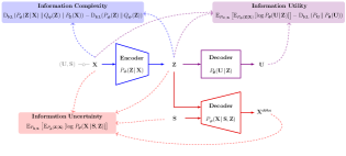
(a)

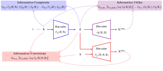
(b)

Figure 4: Block diagram of the DVCLUB associated with $(\text{P1})$ and $(\text{P2})$ in the (a) supervised setup and (b) unsupervised setup.

Consider the lower bound (20) and upper bound (23) on information leakage $\mathrm{I}\left(\mathbf{S};\mathbf{Z}\right)$. Using (30) and (31), the lower and upper bounds on $\mathrm{I}_{\bm{\phi},\bm{\xi}}(\mathbf{S};\mathbf{Z})$ are given as:

$$\mathrm{I}_{\bm{\phi},\bm{\xi}}^{\mathrm{L}}\!\left(\mathbf{S};\mathbf{Z}\right)\!\coloneqq\!-\mathrm{H}_{\bm{\phi},\bm{\xi}}\left(\mathbf{S}\!\mid\!\mathbf{Z}\right)-\mathrm{D}_{\mathrm{KL}}\left(P_{\mathbf{S}}\,\|\,P_{\bm{\xi}}(\mathbf{S})\right)\\ \leq\;\mathrm{I}_{\bm{\phi},\bm{\xi}}(\mathbf{S};\mathbf{Z})\;\leq\;\\ \mathrm{I}_{\bm{\phi},\bm{\psi}}\!\left(\mathbf{X};\mathbf{Z}\right)+\mathrm{H}_{\bm{\phi},\bm{\varphi}}^{\mathrm{U}}\!\left(\mathbf{X}\!\mid\!\mathbf{S},\mathbf{Z}\right)+\mathrm{c}\eqqcolon\mathrm{I}_{\bm{\phi},\bm{\psi},\bm{\varphi}}^{\mathrm{U}}\left(\mathbf{S};\mathbf{Z}\right)+\mathrm{c},$$ (32)

where $\mathrm{c}$ is a constant term, independent of the neural network parameters. The above lower and upper bounds lead us towards two alternative models. The upper bound in (32) encourages the model to directly minimize the information complexity $\mathrm{I}_{\bm{\phi},\bm{\psi}}\!\left(\mathbf{X};\mathbf{Z}\right)$ as well as the information uncertainty $\mathrm{H}_{\bm{\phi},\bm{\varphi}}^{\mathrm{U}}\!\left(\mathbf{X}\!\mid\!\mathbf{S},\mathbf{Z}\right)$. By minimizing the information uncertainty $\mathrm{H}_{\bm{\phi},\bm{\varphi}}^{\mathrm{U}}\!\left(\mathbf{X}\!\mid\!\mathbf{S},\mathbf{Z}\right)$ the model forces to forget the sensitive attribute $\mathbf{S}$ at the expense of reducing the uncertainty about the original data $\mathbf{X}$, i.e., encourages the model to reconstruct the original data $\mathbf{X}$. In contrast, the lower bound in (32) encourages the model to maximizes (i) uncertainty about the sensitive attribute $\mathbf{S}$ given the released representation $\mathbf{Z}$, i.e., $\mathrm{H}_{\bm{\phi},\bm{\xi}}\left(\mathbf{S}\!\mid\!\mathbf{Z}\right)$, as well as (ii) the distribution discrepancy measure $\mathrm{D}_{\mathrm{KL}}\left(P_{\mathbf{S}}\,\|\,P_{\bm{\xi}}(\mathbf{S})\right)$. Note that minimizing the lower bound on information leakage may not necessarily minimize the average maximal possible leakage. Furthermore, although the lower bound in (32) does not explicitly depend on the information complexity $\mathrm{I}_{\bm{\phi},\bm{\psi}}\!\left(\mathbf{X};\mathbf{Z}\right)$, it depends implicitly through the encoder $f_{\bm{\phi}}$.

5.1 DVCLUB Objectives

Considering (12) and (13), and using the addressed parameterized approximations, we have:

$$\mathop{\max}_{P_{\mathbf{Z}\mid\mathbf{X}}}\;\mathop{\max}_{Q_{\mathbf{U}\mid\mathbf{Z}},Q_{\mathbf{Z}},Q_{\mathbf{X}\mid\mathbf{S},\mathbf{Z}}}\;\mathcal{L}_{\mathrm{VCLUB}}^{\mathsf{S/U}}\left(P_{\mathbf{Z}\mid\mathbf{X}},Q_{\mathbf{U}\mid\mathbf{Z}},Q_{\mathbf{Z}},Q_{\mathbf{X}\mid\mathbf{S},\mathbf{Z}},\beta,\alpha\right)\geq\mathop{\max}_{\bm{\phi},\bm{\theta},\bm{\psi},\bm{\varphi}}\mathcal{L}_{\mathrm{DVCLUB}}^{\mathsf{S/U}}\left(\bm{\phi},\bm{\theta},\bm{\psi},\bm{\varphi},\beta,\alpha\right)\!,$$ (33)

or alternatively, we have:

$$\mathop{\min}_{P_{\mathbf{Z}\mid\mathbf{X}}}\;\mathop{\min}_{Q_{\mathbf{U}\mid\mathbf{Z}},Q_{\mathbf{Z}},Q_{\mathbf{X}\mid\mathbf{S},\mathbf{Z}}}\;\mathcal{L}_{\mathrm{VCLUB}}^{\mathsf{S/U}}\left(P_{\mathbf{Z}\mid\mathbf{X}},Q_{\mathbf{U}\mid\mathbf{Z}},Q_{\mathbf{Z}},Q_{\mathbf{X}\mid\mathbf{S},\mathbf{Z}},\gamma,\lambda\right)\leq\mathop{\min}_{\bm{\phi},\bm{\theta},\bm{\psi},\bm{\varphi}}\mathcal{L}_{\mathrm{DVCLUB}}^{\mathsf{S/U}}\left(\bm{\phi},\bm{\theta},\bm{\psi},\bm{\varphi},\gamma,\lambda\right)\!,$$ (34)

where $\mathcal{L}_{\mathrm{DVCLUB}}^{\mathsf{S/U}}\left(\bm{\phi},\bm{\theta},\bm{\psi},\bm{\varphi},\beta,\alpha\right)$ and $\mathcal{L}_{\mathrm{DVCLUB}}^{\mathsf{S/U}}\left(\bm{\phi},\bm{\theta},\bm{\psi},\bm{\varphi},\gamma,\lambda\right)$ denote the associated Deep Variational CLUB (DVCLUB) Lagrangian functionals in the ‘supervised’ or ‘unsupervised’ scenarios, respectively, which are given as:

$$\!\!(\text{P1}\!\!:\!\mathsf{S})\!:\;\mathcal{L}_{\mathrm{DVCLUB}}^{\mathsf{S}}\left(\bm{\phi},\bm{\theta},\bm{\psi},\bm{\varphi},\beta,\alpha\right)\coloneqq\overbrace{\mathbb{E}_{P_{\mathbf{U},\mathbf{X}}}\left[\mathbb{E}_{P_{\bm{\phi}}\left(\mathbf{Z}\mid\mathbf{X}\right)}\left[\log P_{\bm{\theta}}\!\left(\mathbf{U}\!\mid\!\mathbf{Z}\right)\right]\right]-\mathrm{D}_{\mathrm{KL}}\left(P_{\mathbf{U}}\,\|\,P_{\bm{\theta}}(\mathbf{U})\right)}^{{\color[rgb]{.5,0,.5}\mathrm{Information~{}Utility:}~{}\mathrm{I}_{\bm{\phi},\bm{\theta}}^{\mathrm{L}}\left(\mathbf{U};\mathbf{Z}\right)}}\\ \qquad\quad\qquad\quad\qquad\quad\qquad\;\;-\left(\beta+\alpha\right)\!\underbrace{\Big{(}\mathrm{D}_{\mathrm{KL}}\!\left(P_{\bm{\phi}}(\mathbf{Z}\!\mid\!\mathbf{X})\,\|\,Q_{\bm{\psi}}(\mathbf{Z})\mid P_{\mathsf{D}}(\mathbf{X})\right)-\mathrm{D}_{\mathrm{KL}}\!\left(P_{\bm{\phi}}(\mathbf{Z})\,\|\,Q_{\bm{\psi}}(\mathbf{Z})\right)\!\Big{)}}_{{\color[rgb]{0,0,1}\mathrm{Information~{}Complexity:}~{}\mathrm{I}_{\bm{\phi},\bm{\psi}}\left(\mathbf{X};\mathbf{Z}\right)}}\\ \;\;-\,\alpha\,\underbrace{\big{(}-\mathbb{E}_{P_{\mathbf{S},\mathbf{X}}}\left[\mathbb{E}_{P_{\bm{\phi}}\left(\mathbf{Z}\mid\mathbf{X}\right)}\left[\log P_{\bm{\varphi}}\!\left(\mathbf{X}\!\mid\!\mathbf{S},\mathbf{Z}\right)\right]\right]\big{)}}_{{\color[rgb]{1,0,0}\mathrm{Information~{}Uncertainty:}~{}\mathrm{H}_{\bm{\phi},\bm{\varphi}}^{\mathrm{U}}\left(\mathbf{X}\mid\mathbf{S},\mathbf{Z}\right)}}.$$ (35)

$$\!\!(\text{P1}\!\!:\!\mathsf{U})\!:\;\mathcal{L}_{\mathrm{DVCLUB}}^{\mathsf{U}}\left(\bm{\phi},\bm{\theta},\bm{\psi},\bm{\varphi},\beta,\alpha\right)\coloneqq\overbrace{\mathbb{E}_{P_{\mathsf{D}}(\mathbf{X})}\left[\mathbb{E}_{P_{\bm{\phi}}\left(\mathbf{Z}\mid\mathbf{X}\right)}\left[\log P_{\bm{\theta}}\!\left(\mathbf{X}\!\mid\!\mathbf{Z}\right)\right]\right]-\mathrm{D}_{\mathrm{KL}}\left(P_{\mathsf{D}}(\mathbf{X})\,\|\,P_{\bm{\theta}}(\mathbf{X})\right)}^{{\color[rgb]{.5,0,.5}\mathrm{Information~{}Utility:}~{}\mathrm{I}_{\bm{\phi},\bm{\theta}}^{\mathrm{L}}\left(\mathbf{X};\mathbf{Z}\right)}}\\ \qquad\qquad\quad\qquad\qquad\quad\quad\;\;-\left(\beta+\alpha\right)\!\underbrace{\Big{(}\!\mathrm{D}_{\mathrm{KL}}\!\left(P_{\bm{\phi}}(\mathbf{Z}\!\mid\!\mathbf{X})\,\|\,Q_{\bm{\psi}}(\mathbf{Z})\mid P_{\mathsf{D}}(\mathbf{X})\right)-\mathrm{D}_{\mathrm{KL}}\!\left(P_{\bm{\phi}}(\mathbf{Z})\,\|\,Q_{\bm{\psi}}(\mathbf{Z})\right)\!\Big{)}}_{{\color[rgb]{0,0,1}\mathrm{Information~{}Complexity:}~{}\mathrm{I}_{\bm{\phi},\bm{\psi}}\left(\mathbf{X};\mathbf{Z}\right)}}\\ \;\;-\alpha\;\underbrace{\big{(}-\mathbb{E}_{P_{\mathbf{S},\mathbf{X}}}\left[\mathbb{E}_{P_{\bm{\phi}}\left(\mathbf{Z}\mid\mathbf{X}\right)}\left[\log P_{\bm{\varphi}}\!\left(\mathbf{X}\!\mid\!\mathbf{S},\mathbf{Z}\right)\right]\right]\big{)}}_{{\color[rgb]{1,0,0}\mathrm{Information~{}Uncertainty:}~{}\mathrm{H}_{\bm{\phi},\bm{\varphi}}^{\mathrm{U}}\left(\mathbf{X}\mid\mathbf{S},\mathbf{Z}\right)}}\!.\!$$ (36)

Alternatively, one can obtain the DVCLUB Lagrangian functionals associated to (13) in both the supervised and unsupervised scenarios. We will discuss the alternative objectives in Sec. 7. Fig. 4 demonstrates the general block diagram for the supervised and unsupervised DVCLUB models. In practice, we need to train the model using alternating block coordinate descent algorithms. In the following, we gradually build the fundamentals of the learning model.

5.2 Learning Algorithm

Given a collection of i.i.d. training samples $\{\left(\mathbf{u}_{n},\mathbf{s}_{n},\mathbf{x}_{n}\right)\}_{n=1}^{N}\subseteq\mathcal{U}\times\mathcal{S}\times\mathcal{X}$, and using the stochastic gradient descent (SGD)-type algorithms, the deep neural networks $f_{\bm{\phi}}$, $g_{\bm{\theta}}$, and $g_{\bm{\varphi}}$ (or $g_{\bm{\xi}}$) can be trained jointly to maximize a Monte-Carlo approximation of the DVCLUB functionals over parameters $\bm{\phi}$, $\bm{\theta}$, $\bm{\varphi}$, and $\bm{\xi}$. In order to have a stable gradient with respect to the encoder, the reparameterization trick [15] is used to sample from the learned posterior distribution $P_{\bm{\phi}}(\mathbf{Z}\!\mid\!\mathbf{X})$. To do this, we need to explicitly consider $P_{\bm{\phi}}(\mathbf{Z}\!\mid\!\mathbf{X})$ to belong to a tractable parametric family of distributions (e.g., Gaussian distributions) such that we are able to sample from $P_{\bm{\phi}}(\mathbf{Z}\!\!\mid\!\!\mathbf{X})$ by: (i) sampling a random vector $\bm{\mathcal{E}}$ with distribution $P_{\bm{\mathcal{E}}}(\bm{\varepsilon)}$, $\bm{\varepsilon}\in\mathcal{E}$, which does not depend on $\bm{\phi}$; (ii) transforming the samples using some parametric function $f_{\bm{\phi}}:\mathcal{X}\times\mathcal{E}\rightarrow\mathcal{Z}$, such that $\mathbf{Z}=f_{\bm{\phi}}\left(\mathbf{x},\bm{\mathcal{E}}\right)\sim P_{\bm{\phi}}\!\left(\mathbf{Z}\mid\mathbf{X}=\mathbf{x}\right)$. One can consider multivariate Gaussian parametric encoders of mean $\bm{\mu}_{\bm{\phi}}(\mathbf{x})$, and co-variance $\bm{\Sigma}_{\bm{\phi}}(\mathbf{x})$, i.e., $P_{\bm{\phi}}(\mathbf{Z}\!\mid\!\mathbf{x})=\mathcal{N}\left(\bm{\mu}_{\bm{\phi}}(\mathbf{x}),\bm{\Sigma}_{\bm{\phi}}(\mathbf{x})\right)$, where $\bm{\mu}_{\bm{\phi}}(\mathbf{x})$ and $\bm{\Sigma}_{\bm{\phi}}(\mathbf{x})$ are the two output vectors of the network $f_{\bm{\phi}}$ for the given input sample $\mathbf{x}$. The inferred posterior distribution is typically a multi-variate Gaussian with diagonal co-variance, i.e., $P_{\bm{\phi}}(\mathbf{Z}\!\mid\!\mathbf{x})=\mathcal{N}\big{(}\bm{\mu}_{\bm{\phi}}(\mathbf{x}),\mathsf{diag}(\bm{\sigma}_{\bm{\phi}}(\mathbf{x}))\big{)}$. Suppose $\mathcal{Z}=\mathbb{R}^{d_{\mathbf{z}}}$, therefore, we first sample a random variable $\bm{\mathcal{E}}$ i.i.d. from $\mathcal{N}\!\left(\bm{0},\mathbf{I}_{d_{\mathbf{z}}}\right)$, then given a data sample $\mathbf{x}\in\mathcal{X}$, we generate the sample $\mathbf{z}=\bm{\mu}_{\bm{\phi}}(\mathbf{x})+\bm{\sigma}_{\bm{\phi}}(\mathbf{x})\odot\bm{\varepsilon}$, where $\odot$ is the element-wise (Hadamard) product. Noting that $f_{\bm{\phi}}$ is a deterministic mapping, the stochasticity of encoder $P_{\bm{\phi}}\!\left(\mathbf{Z}\!\mid\!\mathbf{X}\right)$ is relegated to the random variable $\bm{\mathcal{E}}$. The decoder $P_{\bm{\theta}}(\mathbf{U}\!\!\mid\!\!\mathbf{Z})$ (likewise $P_{\bm{\theta}}(\mathbf{X}\!\!\mid\!\!\mathbf{Z})$) utilizes a suitable distribution for the data and task under consideration.

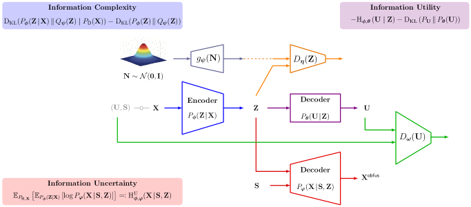
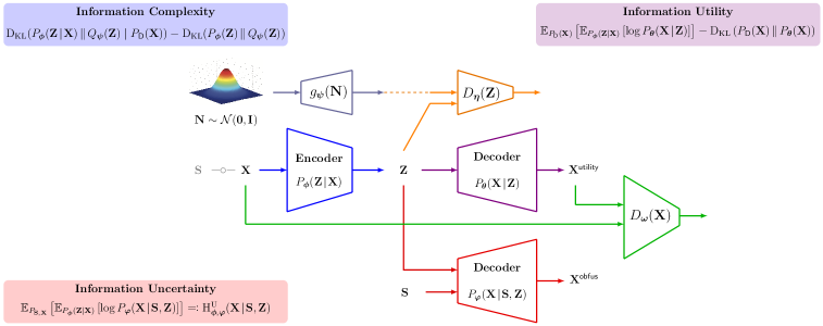
Figure 5: Supervised DVCLUB training architecture associated with $(\text{P1})$.

Figure 6: Unsupervised DVCLUB training architecture associated with $(\text{P1})$.

The latent space prior distribution is typically considered as a fixed $d$-dimensional standard isotropic multi-variate Gaussian, i.e., $Q_{\bm{\psi}}\!\left(\mathbf{Z}\right)=Q_{\mathbf{Z}}=\mathcal{N}\!\left(\bm{0},\mathbf{I}_{d}\right)$. For this simple explicit choice, the information complexity upper bound $\mathbb{E}_{P_{\bm{\phi}}(\mathbf{X},\mathbf{Z})}\big{[}\log\frac{P_{\bm{\phi}}\left(\mathbf{Z}\mid\mathbf{X}\right)}{Q_{\mathbf{Z}}}\big{]}=\mathbb{E}_{P_{\mathsf{D}}(\mathbf{X})}\left[\mathrm{D}_{\mathrm{KL}}\left(P_{\bm{\phi}}\!\left(\mathbf{Z}\!\mid\!\mathbf{X}\right)\|Q_{\mathbf{Z}})\right)\right]$ has a closed-form expression for a given sample $\mathbf{x}$, which reads as $2\,\mathrm{D}_{\mathrm{KL}}\left(P_{\bm{\phi}}\!\left(\mathbf{Z}\!\mid\!\mathbf{X}=\mathbf{x}\right)\|Q_{\mathbf{Z}}\right)={\|\bm{\mu}_{\bm{\phi}}(\mathbf{x})\|}_{2}^{2}+d+\sum_{i=1}^{d}(\bm{\sigma}_{\bm{\phi}}(\mathbf{x})_{i}-\log\bm{\sigma}_{\bm{\phi}}(\mathbf{x})_{i})$. However, simple prior can lead to under-fitting, and, as a consequence, poor representations. On the other hand, having a complete match, i.e., $Q_{\mathbf{Z}}\!=\!\frac{1}{N}\sum_{n=1}^{N}P_{\bm{\phi}}(\mathbf{Z}\!\mid\!\mathbf{x}_{n})$, may potentially lead to over-fitting. Moreover, it is a computationally expensive task due to the summation over all training samples. One possible solution to overcome this issue is to explicitly consider a mixture of diagonal Gaussian distributions as the proposal prior [88, 89], i.e., $Q_{\bm{\psi}}(\mathbf{Z})\!=\!\sum_{k=1}^{K}\pi_{k}\,\mathcal{N}\big{(}\bm{\mu}_{{\bm{\psi}}_{k}},\mathsf{diag}(\bm{\sigma}_{{\bm{\psi}}_{k}})\big{)}$, $\sum_{k=1}^{K}\pi_{k}\!=\!1$, where $K\!\ll\!N$, and learn the mixture weights. In [86], the authors considered the proposal prior as a mixture of equi-probable variational posteriors, such that $Q_{\bm{\psi}}(\mathbf{Z})=\frac{1}{K}\sum_{k=1}^{K}P_{\bm{\phi}}(\mathbf{Z}\!\mid\!\widetilde{\mathbf{x}}_{k})$, where $\{\widetilde{\mathbf{x}}_{k}\}_{k=1}^{K}$, $K\ll N$, are referred to as the pseudo-inputs, which are learned through back-propagation. In the same line of research, in [87], the authors constructed the proposal prior by multiplying a simple prior with a learned acceptance probability function, which re-weights the considered simple prior. Alternatively, one can adversarially learn the prior distribution $Q_{\bm{\psi}}(\mathbf{Z})$ through a generator model $g_{\bm{\psi}}(\mathbf{N})$, where $\mathbf{N}\sim\mathcal{N}\left(\bm{0},\mathbf{I}\right)$. This choice gives us an implicit prior distribution $Q_{\bm{\psi}}(\mathbf{Z})$. Implicit distributions are probability distributions that are learned via passing noise through a deterministic function which is parameterized by a neural network [21, 90, 91, 92, 93]. This allows us easily sample from them and take derivatives of samples with respect to the model parameters.

Divergence Estimation: We can estimate the $\mathrm{KL}$-divergences in (35) and (36) using the density-ratio trick [94, 95], utilized in the GAN framework to directly match the data distribution $P_{\mathbf{X}}$ and the marginal model distribution $P_{\bm{\theta}}(\mathbf{X})$. The trick is to express two distributions as conditional distributions, conditioned on a label $C\in\{0,1\}$, and reduce the task to binary classification. The key point is that we can estimate the KL-divergence, and indeed all the well-defined $f$-divergences, by estimating the ratio of the two distributions without modeling each distribution explicitly. Consider $\mathrm{D}_{\mathrm{KL}}\!\left(P_{\bm{\phi}}(\mathbf{Z})\,\|\,Q_{\bm{\psi}}(\mathbf{Z})\right)=\mathbb{E}_{P_{\bm{\phi}}(\mathbf{Z})}\!\left[\log\frac{P_{\bm{\phi}}(\mathbf{Z})}{Q_{\bm{\psi}}(\mathbf{Z})}\right]$. Define $\rho_{\mathbf{Z}}(\mathbf{z}\mid c)$ as follows:

$$\rho_{\mathbf{Z}}(\mathbf{z}\!\mid\!c)=\left\{\begin{array}[]{ll}P_{\bm{\phi}}(\mathbf{Z})&,~{}\mathrm{if}\quad c=1\\ Q_{\bm{\psi}}(\mathbf{Z})&,~{}\mathrm{if}\quad c=0\end{array}\right..$$ (39)

Suppose that a perfect binary classifier (discriminator) $D_{\bm{\eta}}(\mathbf{z})$, with parameters $\bm{\eta}$, is trained to associate label $c=1$ to samples from distribution $P_{\bm{\phi}}(\mathbf{Z})$ and label $c=0$ to samples from $Q_{\bm{\psi}}(\mathbf{Z})$. Using the Bayes’ rule and assuming that the marginal class probabilities are equal, i.e., $\rho(c=1)=\rho(c=0)$, the density ratio can be expressed as:

$$\frac{P_{\bm{\phi}}(\mathbf{Z}=\mathbf{z})}{Q_{\bm{\psi}}(\mathbf{Z}=\mathbf{z})}=\frac{\rho_{\mathbf{Z}}(\mathbf{z}\mid c=1)}{\rho_{\mathbf{Z}}(\mathbf{z}\mid c=0)}=\frac{\rho_{\mathbf{Z}}(c=1\mid\mathbf{z})}{\rho_{\mathbf{Z}}(c=0\mid\mathbf{z})}\approx\frac{D_{\bm{\eta}}(\mathbf{z})}{1-D_{\bm{\eta}}(\mathbf{z})}.$$ (40)

Therefore, given a trained discriminator $D_{\bm{\eta}}(\mathbf{z})$ and $M$ i.i.d. samples $\{\mathbf{z}_{m}\}_{m=1}^{M}$ from $P_{\bm{\phi}}(\mathbf{Z})$, one can estimate the divergence $\mathrm{D}_{\mathrm{KL}}\!\left(P_{\bm{\phi}}(\mathbf{Z})\,\|\,Q_{\bm{\psi}}(\mathbf{Z})\right)$ as:

$$\mathrm{D}_{\mathrm{KL}}\!\left(P_{\bm{\phi}}(\mathbf{Z})\,\|\,Q_{\bm{\psi}}(\mathbf{Z})\right)\approx\frac{1}{M}\sum_{m=1}^{M}\log\frac{D_{\bm{\eta}}(\mathbf{z}_{m})}{1-D_{\bm{\eta}}(\mathbf{z}_{m})}.$$ (41)

The density ratio trick opens the door to implicit prior and posterior distributions. The implicit generative models provide likelihood-free inference models. Interestingly, this trick allows us to learn the parameterized prior distribution $Q_{\bm{\psi}}(\mathbf{Z})$ through a generator model.

Given the discriminator (parameterized scoring function) $D_{\bm{\eta}}(\mathbf{z})\approx\rho_{\mathbf{Z}}(c=1\mid\mathbf{z})=P_{\bm{\phi}}(\mathbf{Z}=\mathbf{z})$, we now need to specify a proper scoring rule for binary discrimination to allow us for parameter learning. Binary cross-entropy loss is typically considered to this end. In this case, the latent space discriminator $D_{\bm{\eta}}(\mathbf{z})$ minimizes the following loss function:

$$\mathcal{L}_{\mathrm{disc}}^{\mathsf{z}}(\bm{\eta},\bm{\phi}) \coloneqq\mathbb{E}_{\rho_{\mathbf{Z}}(\mathbf{z}\mid c)\rho(c)}\left[\,-c\,\log D_{\bm{\eta}}(\mathbf{Z})-(1-c)\,\log(1-D_{\bm{\eta}}(\mathbf{Z}))\,\right]$$ (42a)

$$=\mathbb{E}_{P_{\mathsf{D}}(\mathbf{X})}\left[\,\mathbb{E}_{P_{\bm{\phi}}(\mathbf{Z}\mid\mathbf{X})}\left[-\log D_{\bm{\eta}}(\mathbf{Z})\right]\,\right]+\mathbb{E}_{Q_{\bm{\psi}}(\mathbf{Z})}\left[\,-\log(1-D_{\bm{\eta}}(\mathbf{Z}))\,\right].$$ (42b)

Analogously, we can estimate the KL-divergence $\mathrm{D}_{\mathrm{KL}}\left(P_{\mathsf{D}}(\mathbf{X})\,\|\,P_{\bm{\theta}}(\mathbf{X})\right)$, the discrepancy measure in the visible (perceptual) space in the unsupervised DVCLUB functional (36). Let us introduce a random variable $y$, and assign a label $y=1$ to sample drawn from $P_{\mathsf{D}}(\mathbf{X})$ and $y=0$ to samples drawn from $P_{\bm{\theta}}(\mathbf{X})$. Also, consider the discriminator $D_{\bm{\omega}}(\mathbf{x})\approx\rho_{\mathbf{X}}(y=1\mid\mathbf{x})=P_{\mathsf{D}}(\mathbf{X}=\mathbf{x})$, with parameters $\bm{\omega}$. Given a trained discriminator $D_{\bm{\omega}}(\mathbf{x})$ and $M$ i.i.d. samples $\{\mathbf{x}_{m}\}_{m=1}^{M}$ from $P_{\mathsf{D}}(\mathbf{X})$, we have:

$$\mathrm{D}_{\mathrm{KL}}\left(P_{\mathsf{D}}(\mathbf{X})\,\|\,P_{\bm{\theta}}(\mathbf{X})\right)\approx\frac{1}{M}\sum_{m=1}^{M}\log\frac{D_{\bm{\omega}}(\mathbf{x}_{m})}{1-D_{\bm{\omega}}(\mathbf{x}_{m})}.$$ (43)

In this case, the visible space discriminator $D_{\bm{\omega}}(\mathbf{x})$ minimizes the following loss function:

$$\mathcal{L}_{\mathrm{disc}}^{\mathsf{x}}(\bm{\omega},\bm{\theta}) \coloneqq\mathbb{E}_{\rho_{\mathbf{X}}(\mathbf{x}\mid y)\rho(y)}\left[\,-y\,\log D_{\bm{\omega}}(\mathbf{X})-(1-y)\,\log(1-D_{\bm{\omega}}(\mathbf{X}))\,\right]$$ (44a)

$$=\mathbb{E}_{P_{\mathsf{D}}(\mathbf{X})}\left[\,-\log D_{\bm{\omega}}(\mathbf{X})\,\right]+\mathbb{E}_{P_{\bm{\theta}}(\mathbf{X})}\left[\,-\log(1-D_{\bm{\omega}}(\mathbf{X}))\,\right]$$ (44b)

$$=\mathbb{E}_{P_{\mathsf{D}}(\mathbf{X})}\left[\,-\log D_{\bm{\omega}}(\mathbf{X})\,\right]+\mathbb{E}_{Q_{\bm{\psi}}(\mathbf{Z})}\left[\,-\log\left(1-D_{\bm{\omega}}(\,g_{\bm{\theta}}(\mathbf{Z})\,)\right)\,\right],$$ (44c)

or equivalently, maximizes $\mathbb{E}_{P_{\mathsf{D}}(\mathbf{X})}\left[\,\log D_{\bm{\omega}}(\mathbf{X})\,\right]+\mathbb{E}_{Q_{\bm{\psi}}(\mathbf{Z})}\left[\,\log\left(1-D_{\bm{\omega}}(\,g_{\bm{\theta}}(\mathbf{Z})\,)\right)\,\right]$.

Learning Procedure: The DVCLUB models $(\text{P1}\!\!:\!\mathsf{S})$ and $(\text{P1}\!\!:\!\mathsf{U})$ are trained using alternating block coordinate descent across five steps:

(1) Train the Encoder, Utility Decoder and Uncertainty Decoder.

• Supervised Setup:

  $$\mathop{\max}_{\bm{\phi},\bm{\theta},\bm{\varphi}}\quad\mathbb{E}_{P_{\mathbf{U},\mathbf{X}}}\left[\mathbb{E}_{P_{\bm{\phi}}(\mathbf{Z}\mid\mathbf{X})}\left[\log P_{\bm{\theta}}(\mathbf{U}\!\mid\!\mathbf{Z})\right]\right]-(\beta+\alpha)\;\;\mathrm{D}_{\mathrm{KL}}\left(P_{\bm{\phi}}(\mathbf{Z}\mid\mathbf{X})\|Q_{\bm{\psi}}(\mathbf{Z})\!\mid\!P_{\mathsf{D}}(\mathbf{X})\right)\\ -\alpha\;\;\mathbb{E}_{P_{\mathbf{S},\mathbf{X}}}\left[\mathbb{E}_{P_{\bm{\phi}}(\mathbf{Z}\mid\mathbf{X})}\left[-\log P_{\bm{\varphi}}(\mathbf{X}\!\mid\!\mathbf{S},\mathbf{Z})\right]\right].$$ (45)

• Unsupervised Setup:

  $$\mathop{\max}_{\bm{\phi},\bm{\theta},\bm{\varphi}}\quad\mathbb{E}_{P_{\mathsf{D}}(\mathbf{X})}\left[\mathbb{E}_{P_{\bm{\phi}}(\mathbf{Z}\mid\mathbf{X})}\left[\log P_{\bm{\theta}}(\mathbf{X}\!\mid\!\mathbf{Z})\right]\right]-(\beta+\alpha)\;\;\mathrm{D}_{\mathrm{KL}}\left(P_{\bm{\phi}}(\mathbf{Z}\mid\mathbf{X})\|Q_{\bm{\psi}}(\mathbf{Z})\!\mid\!P_{\mathsf{D}}(\mathbf{X})\right)\\ -\alpha\;\;\mathbb{E}_{P_{\mathbf{S},\mathbf{X}}}\left[\mathbb{E}_{P_{\bm{\phi}}(\mathbf{Z}\mid\mathbf{X})}\left[-\log P_{\bm{\varphi}}(\mathbf{X}\!\mid\!\mathbf{S},\mathbf{Z})\right]\right].$$ (46)

(2) Train the Latent Space Discriminator.

$$\mathop{\min}_{\bm{\eta}}\quad\mathbb{E}_{P_{\mathsf{D}}(\mathbf{X})}\left[\,\mathbb{E}_{P_{\bm{\phi}}(\mathbf{Z}\mid\mathbf{X})}\left[-\log D_{\bm{\eta}}(\mathbf{Z})\right]\,\right]+\mathbb{E}_{Q_{\bm{\psi}}(\mathbf{Z})}\left[\,-\log(1-D_{\bm{\eta}}(\mathbf{Z}))\,\right].$$ (47)

(3) Train the Encoder and Prior Distribution Generator Adversarially.

$$\mathop{\max}_{\bm{\phi},\bm{\psi}}\quad\mathbb{E}_{P_{\mathsf{D}}(\mathbf{X})}\left[\,\mathbb{E}_{P_{\bm{\phi}}(\mathbf{Z}\mid\mathbf{X})}\left[-\log D_{\bm{\eta}}(\mathbf{Z})\right]\,\right]+\mathbb{E}_{Q_{\bm{\psi}}(\mathbf{Z})}\left[\,-\log(1-D_{\bm{\eta}}(\mathbf{Z}))\,\right].$$ (48)

(4) Train the Output Space Discriminator.

• Supervised Scenario: the Attribute Class Discriminator $D_{\omega}(\mathbf{U})$ is updated as:

  $$\mathop{\min}_{\bm{\omega}}\quad\mathbb{E}_{P_{\mathbf{U}}}\left[\,-\log D_{\bm{\omega}}(\mathbf{U})\,\right]+\mathbb{E}_{Q_{\bm{\psi}}(\mathbf{Z})}\left[\,-\log\left(1-D_{\bm{\omega}}(\,g_{\bm{\theta}}(\mathbf{Z})\,)\right)\,\right].$$ (49)

• Unsupervised Scenario: the Visible Space Discriminator $D_{\omega}(\mathbf{X})$ is updated as:

  $$\mathop{\min}_{\bm{\omega}}\quad\mathbb{E}_{P_{\mathsf{D}}(\mathbf{X})}\left[\,-\log D_{\bm{\omega}}(\mathbf{X})\,\right]+\mathbb{E}_{Q_{\bm{\psi}}(\mathbf{Z})}\left[\,-\log\left(1-D_{\bm{\omega}}(\,g_{\bm{\theta}}(\mathbf{Z})\,)\right)\,\right].$$ (50)

(5) Train the Prior Distribution Generator and Utility Decoder Adversarially.

$$\mathop{\max}_{\bm{\psi},\bm{\theta}}\quad\mathbb{E}_{Q_{\bm{\psi}}(\mathbf{Z})}\left[\,-\log\left(1-D_{\bm{\omega}}(\,g_{\bm{\theta}}(\mathbf{Z})\,)\right)\,\right].$$ (51)

The complete training algorithm of the supervised and unsupervised DVCLUB models are shown in the Algorithm 1 and Algorithm 2, respectively. We will discuss the alternative objectives in Sec. 7, and address their associated training algorithms in Appendix. D. An overview of our implementation is provided in Appendix. C.

1:Input: Training Dataset: $\{\left(\mathbf{u}_{n},\mathbf{s}_{n},\mathbf{x}_{n}\right)\}_{n=1}^{N}$; Hyper-Parameters: $\alpha,\beta$

2:$\bm{\phi},\bm{\theta},\bm{\psi},\bm{\varphi},\bm{\eta},\bm{\omega}\;\leftarrow$ Initialize Network Parameters

3:repeat(1) Train the Encoder, Utility Decoder, Uncertainty Decoder $\left(\bm{\phi},\bm{\theta},\bm{\varphi}\right)$

4:       Sample a mini-batch $\{\mathbf{u}_{m},\mathbf{s}_{m},\mathbf{x}_{m}\}_{m=1}^{M}\sim P_{\mathsf{D}}(\mathbf{X})P_{\mathbf{U},\mathbf{S}\mid\mathbf{X}}$

5:       Compute $\mathbf{z}_{m}\sim f_{\bm{\phi}}(\mathbf{x}_{m}),\forall m\in[M]$

6:       Sample $\{\mathbf{\widehat{z}}_{m}\}_{m=1}^{M}\sim Q_{\bm{\psi}}(\mathbf{Z})$

7:       Compute $\mathbf{\widehat{x}}_{m}=g_{\bm{\varphi}}(\mathbf{\widehat{z}}_{m},\mathbf{s}_{m}),\forall m\in[M]$

8:       Back-propagate loss: $\mathcal{L}\!\left(\bm{\phi},\!\bm{\theta},\!\bm{\varphi}\right)\!=\!\!-\frac{1}{M}\!\sum_{m=1}^{M}\!\!\Big{(}\!\log P_{\bm{\theta}}(\mathbf{u}_{m}\!\mid\!\mathbf{z}_{m})\!-\!(\beta+\alpha)\mathrm{D}_{\mathrm{KL}}\!\left(P_{\bm{\phi}}(\mathbf{z}_{m}\!\mid\!\mathbf{x}_{m})\|Q_{\bm{\psi}}(\mathbf{z}_{m})\right)\!+\!\alpha\log P_{\bm{\varphi}}(\mathbf{\widehat{x}}_{m}\!\mid\!\mathbf{s}_{m},\mathbf{z}_{m})\Big{)}$ (2) Train the Latent Space Discriminator $\bm{\eta}$

9:       Sample $\{\mathbf{x}_{m}\}_{m=1}^{M}\sim P_{\mathsf{D}}(\mathbf{X})$

10:       Sample $\{\mathbf{n}_{m}\}_{m=1}^{M}\sim\mathcal{N}(\bm{0},\mathbf{I})$

11:       Compute $\mathbf{z}_{m}\sim f_{\bm{\phi}}(\mathbf{x}_{m}),\forall m\in[M]$

12:       Compute $\mathbf{\widetilde{z}}_{m}\sim g_{\bm{\psi}}(\mathbf{n}_{m}),\forall m\in[M]$

13:       Back-propagate loss: $\;\;\;\;\mathcal{L}\!\left(\bm{\eta}\right)\!=\!\left(\beta+\alpha\right)\left[-\frac{1}{M}\sum_{m=1}^{M}\!\Big{(}\log D_{\bm{\eta}}(\mathbf{z}_{m})+\log\left(1-D_{\bm{\eta}}(\,\mathbf{\widetilde{z}}_{m}\,)\right)\Big{)}\right]$ (3) Train the Encoder and Prior Distribution Generator $\left(\bm{\phi},\bm{\psi}\right)$ Adversarially

14:       Sample $\{\mathbf{x}_{m}\}_{m=1}^{M}\sim P_{\mathsf{D}}(\mathbf{X})$

15:       Sample $\{\mathbf{n}_{m}\}_{m=1}^{M}\sim\mathcal{N}(\bm{0},\mathbf{I})$

16:       Compute $\mathbf{z}_{m}\sim f_{\bm{\phi}}(\mathbf{x}_{m}),\forall m\in[M]$

17:       Compute $\mathbf{\widetilde{z}}_{m}\sim g_{\bm{\psi}}(\mathbf{n}_{m}),\forall m\in[M]$

18:       Back-propagate loss: $\;\;\;\;\mathcal{L}\!\left(\bm{\phi},\bm{\psi}\right)\!=\!\left(\beta+\alpha\right)\left[\frac{1}{M}\sum_{m=1}^{M}\!\Big{(}\log D_{\bm{\eta}}(\mathbf{z}_{m})+\log\left(1-D_{\bm{\eta}}(\,\mathbf{\widetilde{z}}_{m}\,)\right)\Big{)}\right]$ (4) Train the Attribute Class Discriminator $\bm{\omega}$

19:       Sample $\{\mathbf{u}_{m}\}_{m=1}^{M}\sim P_{\mathbf{U}}$

20:       Sample $\{\mathbf{n}_{m}\}_{m=1}^{M}\sim\mathcal{N}\!\left(\bm{0},\mathbf{I}\right)$

21:       Compute $\mathbf{\widetilde{u}}_{m}\sim g_{\bm{\theta}}\left(g_{\bm{\psi}}(\mathbf{n}_{m})\right),\forall m\in[M]$

22:       Back-propagate loss: $\;\;\;\;\mathcal{L}\!\left(\bm{\omega}\right)\!=\!-\frac{1}{M}\sum_{m=1}^{M}\!\Big{(}\log D_{\bm{\omega}}(\mathbf{u}_{m})+\log\left(1-D_{\bm{\omega}}(\,\mathbf{\widetilde{u}}_{m}\,)\right)\Big{)}$ (5) Train the Prior Distribution Generator and Utility Decoder $\left(\bm{\psi},\bm{\theta}\right)$ Adversarially

23:       Sample $\{\mathbf{n}_{m}\}_{m=1}^{M}\sim\mathcal{N}\!\left(\bm{0},\mathbf{I}\right)$

24:       Compute $\mathbf{\widetilde{u}}_{m}\sim g_{\bm{\theta}}\left(g_{\bm{\psi}}(\mathbf{n}_{m})\right),\forall m\in[M]$

25:       Back-propagate loss: $\;\;\;\;\mathcal{L}\!\left(\bm{\psi},\bm{\theta}\right)\!=\!\frac{1}{M}\sum_{m=1}^{M}\!\log\left(1-D_{\bm{\omega}}(\,\mathbf{\widetilde{u}}_{m}\,)\right)$

26:until Convergence

27:return $\bm{\phi},\bm{\theta},\bm{\psi},\bm{\varphi},\bm{\eta},\bm{\omega}$

Algorithm 1 Supervised Deep Variational CLUB training algorithm associated with ($\text{P1}\!\!:\!\mathsf{S}$)

1:Input: Training Dataset: $\{\left(\mathbf{s}_{n},\mathbf{x}_{n}\right)\}_{n=1}^{N}$; Hyper-Parameters: $\alpha,\beta$

2:$\bm{\phi},\bm{\theta},\bm{\psi},\bm{\varphi},\bm{\eta},\bm{\omega}\;\leftarrow$ Initialize Network Parameters

3:repeat(1) Train the Encoder, Utility Decoder, Uncertainty Decoder $\left(\bm{\phi},\bm{\theta},\bm{\varphi}\right)$

4:       Sample a mini-batch $\{\mathbf{s}_{m},\mathbf{x}_{m}\}_{m=1}^{M}\sim P_{\mathsf{D}}(\mathbf{X})P_{\mathbf{S}\mid\mathbf{X}}$

5:       Compute $\mathbf{z}_{m}\sim f_{\bm{\phi}}(\mathbf{x}_{m}),\forall m\in[M]$

6:       Sample $\{\mathbf{\widehat{z}}_{m}\}_{m=1}^{M}\sim Q_{\bm{\psi}}(\mathbf{Z})$

7:       Compute $\mathbf{\widehat{x}}_{m}=g_{\bm{\varphi}}(\mathbf{\widehat{z}}_{m},\mathbf{s}_{m}),\forall m\in[M]$

8:       Back-propagate loss: $\mathcal{L}\!\left(\bm{\phi},\!\bm{\theta},\!\bm{\varphi}\right)\!=\!\!-\frac{1}{M}\!\sum_{m=1}^{M}\!\!\Big{(}\!\log P_{\bm{\theta}}(\mathbf{x}_{m}\!\mid\!\mathbf{z}_{m})\!-\!(\beta+\alpha)\mathrm{D}_{\mathrm{KL}}\!\left(P_{\bm{\phi}}(\mathbf{z}_{m}\!\mid\!\mathbf{x}_{m})\|Q_{\bm{\psi}}(\mathbf{z}_{m})\right)\!+\!\alpha\log P_{\bm{\varphi}}(\mathbf{\widehat{x}}_{m}\!\mid\!\mathbf{s}_{m},\mathbf{z}_{m})\Big{)}$ (2) Train the Latent Space Discriminator $\bm{\eta}$

9:       Sample $\{\mathbf{x}_{m}\}_{m=1}^{M}\sim P_{\mathsf{D}}(\mathbf{X})$

10:       Sample $\{\mathbf{n}_{m}\}_{m=1}^{M}\sim\mathcal{N}(\bm{0},\mathbf{I})$

11:       Compute $\mathbf{z}_{m}\sim f_{\bm{\phi}}(\mathbf{x}_{m}),\forall m\in[M]$

12:       Compute $\mathbf{\widetilde{z}}_{m}\sim g_{\bm{\psi}}(\mathbf{n}_{m}),\forall m\in[M]$

13:       Back-propagate loss: $\;\;\;\;\mathcal{L}\!\left(\bm{\eta}\right)\!=\!\left(\beta+\alpha\right)\left[-\frac{1}{M}\sum_{m=1}^{M}\!\big{(}\,\log D_{\bm{\eta}}(\mathbf{z}_{m})+\log\left(1-D_{\bm{\eta}}(\,\mathbf{\widetilde{z}}_{m}\,)\right)\,\big{)}\right]$ (3) Train the Encoder and Prior Distribution Generator $\left(\bm{\phi},\bm{\psi}\right)$ Adversarially

14:       Sample $\{\mathbf{x}_{m}\}_{m=1}^{M}\sim P_{\mathsf{D}}(\mathbf{X})$

15:       Sample $\{\mathbf{n}_{m}\}_{m=1}^{M}\sim\mathcal{N}(\bm{0},\mathbf{I})$

16:       Compute $\mathbf{z}_{m}\sim f_{\bm{\phi}}(\mathbf{x}_{m}),\forall m\in[M]$

17:       Compute $\mathbf{\widetilde{z}}_{m}\sim g_{\bm{\psi}}(\mathbf{n}_{m}),\forall m\in[M]$

18:       Back-propagate loss: $\;\;\;\;\mathcal{L}\!\left(\bm{\phi},\bm{\psi}\right)\!=\!\left(\beta+\alpha\right)\left[\frac{1}{M}\sum_{m=1}^{M}\!\big{(}\,\log D_{\bm{\eta}}(\mathbf{z}_{m})+\log\left(1-D_{\bm{\eta}}(\,\mathbf{\widetilde{z}}_{m}\,)\right)\,\big{)}\right]$ (4) Train the Visible Space Discriminator $\bm{\omega}$

19:       Sample $\{\mathbf{x}_{m}\}_{m=1}^{M}\sim P_{\mathsf{D}}(\mathbf{X})$

20:       Sample $\{\mathbf{n}_{m}\}_{m=1}^{M}\sim\mathcal{N}\!\left(\bm{0},\mathbf{I}\right)$

21:       Compute $\mathbf{\widetilde{x}}_{m}\sim g_{\bm{\theta}}(g_{\bm{\psi}}(\mathbf{n}_{m})),\forall m\in[M]$

22:       Back-propagate loss: $\;\;\;\;\mathcal{L}\!\left(\bm{\omega}\right)\!=\!-\frac{1}{M}\sum_{m=1}^{M}\!\Big{(}\,\log D_{\bm{\omega}}(\mathbf{x}_{m})+\log\left(1-D_{\bm{\omega}}(\,\mathbf{\widetilde{x}}_{m}\,)\,\right)\Big{)}$ (5) Train the Prior Distribution Generator and Utility Decoder $\left(\bm{\psi},\bm{\theta}\right)$ Adversarially

23:       Sample $\{\mathbf{n}_{m}\}_{m=1}^{M}\sim\mathcal{N}\!\left(\bm{0},\mathbf{I}\right)$

24:       Compute $\mathbf{\widetilde{x}}_{m}\sim g_{\bm{\theta}}\left(g_{\bm{\psi}}(\mathbf{n}_{m})\right),\forall m\in[M]$

25:       Back-propagate loss: $\;\;\;\;\mathcal{L}\!\left(\bm{\psi},\bm{\theta}\right)\!=\!\frac{1}{M}\sum_{m=1}^{M}\log\left(1-D_{\bm{\omega}}(\,\mathbf{\widetilde{x}}_{m}\,)\right)$

26:until Convergence

27:return $\bm{\phi},\bm{\theta},\bm{\psi},\bm{\varphi},\bm{\eta},\bm{\omega}$

Algorithm 2 Unsupervised Deep Variational CLUB training algorithm associated with ($\text{P1}\!\!:\!\mathsf{U}$)

6 Connections with other Problems

6.1 Connection with State-of-the-Art Bottleneck Models

In this subsection, we present the connection of CLUB model with the most relative state-of-the-art literature. We show that CLUB model generalizes most of the previously proposed models. To help interpretation, we use $\mathrm{I}$-Diagram [96], an analogy between information theory and set theory, to visualize a clear connection between the different considered objectives. By constructing an unique measure, called $\mathrm{I}$-Measure, consistent with Shannon’s information measure, we can geometrically represent the relationship among the Shannon’s information measures. The Markov chain $\left(\mathbf{U},\mathbf{S}\right)\hbox{$\--$}\kern-1.5pt\hbox{$\circ$}\kern-1.5pt\hbox{$\--$}\mathbf{X}\hbox{$\--$}\kern-1.5pt\hbox{$\circ$}\kern-1.5pt\hbox{$\--$}\mathbf{Z}$ implies:

$$\mathrm{I}\left(\mathbf{U};\mathbf{S};\mathbf{Z}\mid\mathbf{X}\right)+\mathrm{I}\left(\mathbf{U};\mathbf{Z}\mid\mathbf{S},\mathbf{X}\right)+\mathrm{I}\left(\mathbf{S};\mathbf{Z}\mid\mathbf{U},\mathbf{X}\right)\!\! = \!\!\mathrm{I}\left(\mathbf{U};\mathbf{Z}\mid\mathbf{X}\right)+\mathrm{I}\left(\mathbf{S};\mathbf{Z}\mid\mathbf{U},\mathbf{X}\right)$$ (52)

$$= \!\!\mathrm{I}\left(\mathbf{U},\mathbf{S};\mathbf{Z}\mid\mathbf{X}\right)=0.$$

Considering the Markov chain $\left(\mathbf{U},\mathbf{S}\right)\hbox{$\--$}\kern-1.5pt\hbox{$\circ$}\kern-1.5pt\hbox{$\--$}\mathbf{X}\hbox{$\--$}\kern-1.5pt\hbox{$\circ$}\kern-1.5pt\hbox{$\--$}\mathbf{Z}$, the corresponding $\mathrm{I}$-Diagram is depicted in Fig. 7, where various information quantities are also highlighted.

Information Bottleneck (IB). The IB principle [3] formulates the problem of extracting the relevant information from the random variable $\mathbf{X}$ about the random variable $\mathbf{U}$ that is of interest. Given two correlated random variables $\mathbf{U}$ and $\mathbf{X}$ with joint distribution $P_{\mathbf{U,X}}$, the goal of original IB is to find a representation $\mathbf{Z}$ of $\mathbf{X}$ using a stochastic mapping $P_{\mathbf{Z}\mid\mathbf{X}}$ such that: (i) $\mathbf{U}\hbox{$\--$}\kern-1.5pt\hbox{$\circ$}\kern-1.5pt\hbox{$\--$}\mathbf{X}\hbox{$\--$}\kern-1.5pt\hbox{$\circ$}\kern-1.5pt\hbox{$\--$}\mathbf{Z}$ and (ii) representation $\mathbf{Z}$ is maximally informative about $\mathbf{U}$ (maximizing $\mathrm{I}\left(\mathbf{U};\mathbf{Z}\right)$) while being minimally informative about $\mathbf{X}$ (minimizing $\mathrm{I}\left(\mathbf{X};\mathbf{Z}\right)$). This trade-off can be formulated by bottleneck functional:

$$\mathsf{IB}\left(R,P_{\mathbf{U},\mathbf{X}}\right)\coloneqq\mathop{\sup}_{\begin{subarray}{c}P_{\mathbf{Z}\mid\mathbf{X}}:\\ \mathbf{U}\hbox{$\--$}\kern-1.5pt\hbox{$\circ$}\kern-1.5pt\hbox{$\--$}\mathbf{X}\hbox{$\--$}\kern-1.5pt\hbox{$\circ$}\kern-1.5pt\hbox{$\--$}\mathbf{Z}\end{subarray}}\mathrm{I}\left(\mathbf{U};\mathbf{Z}\right)\;\;\mathrm{s.t.}\;\;\mathrm{I}\left(\mathbf{X};\mathbf{Z}\right)\leq R.$$ (53)

In IB model, $\mathrm{I}\left(\mathbf{U};\mathbf{Z}\right)$ is referred to as the relevance of $\mathbf{Z}$ and $\mathrm{I}\left(\mathbf{X};\mathbf{Z}\right)$ is referred to as the complexity of $\mathbf{Z}$. The values $\mathsf{IB}\left(R,P_{\mathbf{U},\mathbf{X}}\right)$ for different $R$ specify the IB curve. Analogously, with the introduction of a Lagrange multiplier $\beta\in\left[0,1\right]$ we can quantify the IB problem by the associated Lagrangian functional $\mathcal{L}_{\mathrm{IB}}\left(P_{\mathbf{Z}\mid\mathbf{X}},\beta\right)\coloneqq\mathrm{I}\left(\mathbf{U};\mathbf{Z}\right)-\beta\,\mathrm{I}\left(\mathbf{X};\mathbf{Z}\right)$. Clearly, IB is a specific case of CLUB model (7), when the information leakage is disregarded, or equivalently, when $R^{\mathrm{s}}\geq\mathrm{H}\left(\mathbf{S}\right)$.

The underlying IB optimization problem dates back to the early 1970’s, when Wyner and Ziv [97] determined the value of IB functional (53) for the special case of binary random variables. See also [98, 99, 100] for the related problems. Inspired by the formulation of IB method in [3], abundant characterizations, generalizations, and applications have been proposed [2, 101, 102, 103, 104, 105, 106, 107, 108, 109, 81, 110, 111, 112, 113, 114]. We refer the reader to [115, 116, 117, 118] for a review of recent research on IB models.

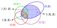
(a)

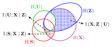
(b)

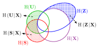
(c)

Figure 7: Information diagrams for $\left(\mathbf{U},\mathbf{S}\right)\hbox{$\--$}\kern-1.5pt\hbox{$\circ$}\kern-1.5pt\hbox{$\--$}\mathbf{X}\hbox{$\--$}\kern-1.5pt\hbox{$\circ$}\kern-1.5pt\hbox{$\--$}\mathbf{Z}$. (a) mutual information $\mathrm{I}\left(\mathbf{U};\mathbf{Z}\right)$, $\mathrm{I}\left(\mathbf{X};\mathbf{Z}\right)$ and $\mathrm{I}\left(\mathbf{S};\mathbf{Z}\right)$; (b) redundant information $\mathrm{I}\left(\mathbf{X};\mathbf{Z}\mid\mathbf{U}\right)$, residual information $\mathrm{I}\left(\mathbf{U};\mathbf{X}\mid\mathbf{Z}\right)$ and residual information $\mathrm{I}\left(\mathbf{S};\mathbf{X}\mid\mathbf{Z}\right)$; (c) utility attribute uncertainty $\mathrm{H}\left(\mathbf{U}\!\mid\!\mathbf{X}\right)$, private attribute uncertainty $\mathrm{H}\left(\mathbf{S}\!\mid\!\mathbf{X}\right)$ and encoding uncertainty $\mathrm{H}\left(\mathbf{Z}\!\mid\!\mathbf{X}\right)$.

Privacy Funnel (PF). In contrast to IB principle, which seeks to obtain a representation $\mathbf{Z}$ that is maximally expressive (information preserving) about $\mathbf{U}$ while maximally compressive about $\mathbf{X}$, considering Markov chain $\mathbf{S}\hbox{$\--$}\kern-1.5pt\hbox{$\circ$}\kern-1.5pt\hbox{$\--$}\mathbf{X}\hbox{$\--$}\kern-1.5pt\hbox{$\circ$}\kern-1.5pt\hbox{$\--$}\mathbf{Z}$, the goal of PF [2] is to determine a representation $\mathbf{Z}$ that minimizes the information leakage between the private (sensitive) data $\mathbf{S}$ and the disclosed representation $\mathbf{Z}$, i.e., $\mathrm{I}\left(\mathbf{S};\mathbf{Z}\right)$, while maximizes the amount of information between non-private (useful) data $\mathbf{X}$ and disclosed representation $\mathbf{Z}$, i.e., $\mathrm{I}\left(\mathbf{X};\mathbf{Z}\right)$. Therefore, the PF method addresses the trade-off between the information leakage $\mathrm{I}\left(\mathbf{S};\mathbf{Z}\right)$ and the revealed useful information $\mathrm{I}\left(\mathbf{X};\mathbf{Z}\right)$. Analogously, this trade-off can be formulated by the PF functional:

$$\mathsf{PF}\left(R,P_{\mathbf{S},\mathbf{X}}\right)\coloneqq\mathop{\inf}_{\begin{subarray}{c}P_{\mathbf{Z}\mid\mathbf{X}}:\\ \mathbf{S}\hbox{$\--$}\kern-1.5pt\hbox{$\circ$}\kern-1.5pt\hbox{$\--$}\mathbf{X}\hbox{$\--$}\kern-1.5pt\hbox{$\circ$}\kern-1.5pt\hbox{$\--$}\mathbf{Z}\end{subarray}}\mathrm{I}\left(\mathbf{S};\mathbf{Z}\right)\;\;\mathrm{s.t.}\;\;\mathrm{I}\left(\mathbf{X};\mathbf{Z}\right)\geq R.$$ (54)

The values $\mathsf{PF}\left(R,P_{\mathbf{S},\mathbf{X}}\right)$ for different $R$ specify the PF curve. By introducing a Lagrange multiplier $\beta\in\left[0,1\right]$ we can quantify the PF problem by the associated Lagrangian functional $\mathcal{L}_{\mathrm{PF}}\left(P_{\mathbf{Z}\mid\mathbf{X}},\beta\right)\coloneqq\mathrm{I}\left(\mathbf{S};\mathbf{Z}\right)-\beta\,\mathrm{I}\left(\mathbf{X};\mathbf{Z}\right)$. Setting $\mathbf{U}\equiv\mathbf{X}$ and $R^{\mathrm{z}}\geq\mathrm{H}\left(P_{\mathbf{X}}\right)$ in the CLUB objective (7), the CLUB model reduces to the PF model. This corresponds to a scenario, for instance, in which the goal is to release facial images, without revealing a specific sensitive attribute.

In [62], the authors obtained a map $P_{\mathbf{Z}\mid\mathbf{X}}$ that minimizes $\mathrm{I}\left(\mathbf{U};\mathbf{X}\mid\mathbf{Z}\right)$ under an information leakage constraint $\mathrm{I}\left(\mathbf{S};\mathbf{Z}\right)$. Considering a similar setting to ours, the following objective is considered:

$$\mathop{\inf}_{\begin{subarray}{c}P_{\mathbf{Z}\mid\mathbf{X}}:\\ \left(\mathbf{U},\mathbf{S}\right)\hbox{$\--$}\kern-1.5pt\hbox{$\circ$}\kern-1.5pt\hbox{$\--$}\mathbf{X}\hbox{$\--$}\kern-1.5pt\hbox{$\circ$}\kern-1.5pt\hbox{$\--$}\mathbf{Z}\end{subarray}}\quad\mathrm{I}\left(\mathbf{U};\mathbf{X}\mid\mathbf{Z}\right)\quad\mathrm{s.t.}\quad\mathrm{I}\left(\mathbf{S};\mathbf{Z}\right)\leq R^{\mathrm{s}}.$$ (55)

One can interpret $\mathrm{I}\left(\mathbf{U};\mathbf{X}\mid\mathbf{Z}\right)$ as the amount of information about $\mathbf{U}$ we lose by observing the released representation $\mathbf{Z}$ instead of the original data $\mathbf{X}$. To see its connection to CLUB, note that, under the Markov chain $\mathbf{U}\hbox{$\--$}\kern-1.5pt\hbox{$\circ$}\kern-1.5pt\hbox{$\--$}\mathbf{X}\hbox{$\--$}\kern-1.5pt\hbox{$\circ$}\kern-1.5pt\hbox{$\--$}\mathbf{Z}$, we have:

$$\mathrm{I}\left(\mathbf{U};\mathbf{Z}\right)=\mathrm{I}\left(\mathbf{U};\mathbf{X}\right)-\mathrm{I}\left(\mathbf{U};\mathbf{X}\mid\mathbf{Z}\right).$$ (56)

Therefore, maximizing $\mathrm{I}\left(\mathbf{U};\mathbf{Z}\right)$ is equivalent to minimizing $\mathrm{I}\left(\mathbf{U};\mathbf{X}\mid\mathbf{Z}\right)$. Clearly, the objective (55) can be considered as a special case of the CLUB model in (7). In particular, we highlight that our model addresses the key missed component in the considered formulation, i.e., the information complexity constraint.

Note that $P_{\mathbf{U},\mathbf{X}\mid\mathbf{Z}}=P_{\mathbf{U}\mid\mathbf{X},\mathbf{Z}}P_{\mathbf{X}\mid\mathbf{Z}}=P_{\mathbf{U}\mid\mathbf{X}}P_{\mathbf{X}\mid\mathbf{Z}}$, hence,

$$\mathrm{I}\left(\mathbf{U};\mathbf{X}\mid\mathbf{Z}\right) = \mathbb{E}_{P_{\mathbf{U},\mathbf{X},\mathbf{Z}}}\left[\log\frac{P_{\mathbf{U},\mathbf{X}\mid\mathbf{Z}}}{P_{\mathbf{U}\mid\mathbf{Z}}P_{\mathbf{X}\mid\mathbf{Z}}}\right]=\mathbb{E}_{P_{\mathbf{U},\mathbf{X},\mathbf{Z}}}\left[\log\frac{P_{\mathbf{U}\mid\mathbf{X}}P_{\mathbf{X}\mid\mathbf{Z}}}{P_{\mathbf{U}\mid\mathbf{Z}}P_{\mathbf{X}\mid\mathbf{Z}}}\right]=\mathbb{E}_{P_{\mathbf{X},\mathbf{Z}}}\Big{[}\mathbb{E}_{P_{\mathbf{U}\mid\mathbf{X},\mathbf{Z}}}\big{[}\log\frac{P_{\mathbf{U}\mid\mathbf{X}}}{P_{\mathbf{U}\mid\mathbf{Z}}}\big{]}\Big{]}$$ (57)

$$= \mathbb{E}_{P_{\mathbf{X},\mathbf{Z}}}\left[\mathrm{D}_{\mathrm{KL}}\left(P_{\mathbf{U}\mid\mathbf{X}}\|P_{\mathbf{U}\mid\mathbf{Z}}\right)\right].$$

This gives us another interpretation of the CLUB objective as a distribution matching problem, which aims at obtaining a stochastic map $P_{\mathbf{Z}\mid\mathbf{X}}$ such that $P_{\mathbf{U}\mid\mathbf{Z}}\approx P_{\mathbf{U}\mid\mathbf{X}}$. This means that the posterior distributions of the utility attribute $\mathbf{U}$ are similar conditioned on the released representation $\mathbf{Z}$ or the original data $\mathbf{X}$. Finally, we remark that Eq. (56) is also related to the source coding problem with a common reconstruction constraint studied in [119, 120].

Deterministic IB (DIB). In the information complexity decomposition $\mathrm{I}\left(\mathbf{X};\mathbf{Z}\right)=\mathrm{H}\left(\mathbf{Z}\right)-\mathrm{H}\left(\mathbf{Z}\mid\mathbf{X}\right)$, the conditional entropy $\mathrm{H}\left(\mathbf{Z}\!\mid\!\mathbf{X}\right)$ measures the encoding uncertainty (see Fig. 7(c)). The deterministic IB model [103] is based on a deterministic encoder. In this case, we have $\mathrm{H}\left(\mathbf{Z}\!\mid\!\mathbf{X}\right)=0$. Considering the Markov chain $\mathbf{U}\hbox{$\--$}\kern-1.5pt\hbox{$\circ$}\kern-1.5pt\hbox{$\--$}\mathbf{X}\hbox{$\--$}\kern-1.5pt\hbox{$\circ$}\kern-1.5pt\hbox{$\--$}\mathbf{Z}$, the following objective is considered:

$$\mathsf{DIB}\left(R,P_{\mathbf{U},\mathbf{X}}\right)\coloneqq\mathop{\inf}_{\begin{subarray}{c}P_{\mathbf{Z}\mid\mathbf{X}}:\\ \mathbf{U}\hbox{$\--$}\kern-1.5pt\hbox{$\circ$}\kern-1.5pt\hbox{$\--$}\mathbf{X}\hbox{$\--$}\kern-1.5pt\hbox{$\circ$}\kern-1.5pt\hbox{$\--$}\mathbf{Z}\end{subarray}}\quad\mathrm{H}\left(\mathbf{Z}\right)\quad\mathrm{s.t.}\quad\mathrm{I}\left(\mathbf{U};\mathbf{Z}\right)\geq R.$$ (58)

In this case, the associated Lagrangian functional is given by $\mathcal{L}_{\mathrm{DIB}}(P_{\mathbf{Z}\mid\mathbf{X}},\beta)\coloneqq\mathrm{H}\left(\mathbf{Z}\right)-\beta\mathrm{I}\left(\mathbf{U};\mathbf{Z}\right)$. Clearly, DIB is a specific case of the IB model; and hence, the CLUB model in (8).

Conditional Entropy Bottleneck (CEB). The conditional entropy bottleneck (CEB) [81] is motivated from the principle of minimum necessary information, and considers the following objective:

$$\mathsf{CEB}\left(R,P_{\mathbf{U},\mathbf{X}}\right)\coloneqq\mathop{\sup}_{\begin{subarray}{c}P_{\mathbf{Z}\mid\mathbf{X}}:\\ \mathbf{U}\hbox{$\--$}\kern-1.5pt\hbox{$\circ$}\kern-1.5pt\hbox{$\--$}\mathbf{X}\hbox{$\--$}\kern-1.5pt\hbox{$\circ$}\kern-1.5pt\hbox{$\--$}\mathbf{Z}\end{subarray}}\quad\mathrm{I}\left(\mathbf{U};\mathbf{Z}\right)\quad\mathrm{s.t.}\quad\mathrm{I}\left(\mathbf{X};\mathbf{Z}\mid\mathbf{U}\right)\leq R.$$ (59)

One can interpret $\mathrm{I}\left(\mathbf{X};\mathbf{Z}\mid\mathbf{U}\right)$ as the redundant information in the released representation $\mathbf{Z}$ about the utility attribute $\mathbf{U}$. To see its connection to CLUB, let us consider the Markov chain $\mathbf{U}\hbox{$\--$}\kern-1.5pt\hbox{$\circ$}\kern-1.5pt\hbox{$\--$}\mathbf{X}\hbox{$\--$}\kern-1.5pt\hbox{$\circ$}\kern-1.5pt\hbox{$\--$}\mathbf{Z}$, we have:

$$\mathrm{I}\left(\mathbf{X};\mathbf{Z}\right)=\mathrm{I}\left(\mathbf{X};\mathbf{Z}\mid\mathbf{U}\right)+\mathrm{I}\left(\mathbf{U};\mathbf{Z}\right).$$ (60)

Therefore, using (60), the associated CEB Lagrangian $\mathcal{L}_{\mathrm{CEB}}\left(P_{\mathbf{Z}\mid\mathbf{X}},\beta^{\prime}\right)\coloneqq\mathrm{I}\left(\mathbf{U};\mathbf{Z}\right)-\beta^{\prime}\,\mathrm{I}\left(\mathbf{X};\mathbf{Z}\mid\mathbf{U}\right)$ can recast as:

$$\mathcal{L}_{\mathrm{CEB}}\left(P_{\mathbf{Z}\mid\mathbf{X}},\beta^{\prime}\right) = \left(\beta^{\prime}+1\right)\mathrm{I}\left(\mathbf{U};\mathbf{Z}\right)-\beta^{\prime}\mathrm{I}\left(\mathbf{X};\mathbf{Z}\right)$$ (61)

$$= \left(\beta^{\prime}+1\right)\Big{(}\mathrm{I}\left(\mathbf{S};\mathbf{Z}\right)-\frac{\beta^{\prime}}{\beta^{\prime}+1}\mathrm{I}\left(\mathbf{X};\mathbf{Z}\right)\Big{)}$$

$$= \left(\beta^{\prime}+1\right)\mathcal{L}_{\mathrm{IB}}\left(P_{\mathbf{Z}\mid\mathbf{X}},\beta\right),$$

where $\beta=\beta^{\prime}/(\beta^{\prime}+1)$. Hence, maximizing $\mathcal{L}_{\mathrm{CEB}}\left(P_{\mathbf{Z}\mid\mathbf{X}},\beta^{\prime}\right)$ is equivalent to maximizing $\mathcal{L}_{\mathrm{IB}}\left(P_{\mathbf{Z}\mid\mathbf{X}},\beta\right)$, which is a specific case of CLUB model (7).

Conditional PF (CPF). Inspired by the conditional entropy bottleneck [81] and noting that the PF (54) is dual of the Information Bottleneck (53), the recent work of [82], addressed the CPF as:

$$\mathsf{CPF}\left(R,P_{\mathbf{S},\mathbf{X}}\right)\coloneqq\mathop{\inf}_{\begin{subarray}{c}P_{\mathbf{Z}\mid\mathbf{X}}:\\ \mathbf{S}\hbox{$\--$}\kern-1.5pt\hbox{$\circ$}\kern-1.5pt\hbox{$\--$}\mathbf{X}\hbox{$\--$}\kern-1.5pt\hbox{$\circ$}\kern-1.5pt\hbox{$\--$}\mathbf{Z}\end{subarray}}\quad\mathrm{I}\left(\mathbf{S};\mathbf{Z}\right)\quad\mathrm{s.t.}\quad\mathrm{I}\left(\mathbf{X};\mathbf{Z}\mid\mathbf{S}\right)\geq R^{\mathrm{c}\mid\mathrm{s}}.$$ (62)

To see its connection to CLUB, we use the Markov chain $\mathbf{S}\hbox{$\--$}\kern-1.5pt\hbox{$\circ$}\kern-1.5pt\hbox{$\--$}\mathbf{X}\hbox{$\--$}\kern-1.5pt\hbox{$\circ$}\kern-1.5pt\hbox{$\--$}\mathbf{Z}$ to obtain:

$$\mathrm{I}\left(\mathbf{X};\mathbf{Z}\right)=\mathrm{I}\left(\mathbf{X};\mathbf{Z}\mid\mathbf{S}\right)+\mathrm{I}\left(\mathbf{S};\mathbf{Z}\right).$$ (63)

Hence, CPF ignores the shared information in the released representation $\mathbf{Z}$ about the private attribute $\mathbf{S}$, and imposes the constraint on the residual information in the released representation $\mathbf{Z}$ about the useful data $\mathbf{X}$. The associated CPF Lagrangian functional is given by $\mathcal{L}_{\mathrm{CPF}}\left(P_{\mathbf{Z}\mid\mathbf{X}},\beta^{\prime}\right)\coloneqq\mathrm{I}\left(\mathbf{S};\mathbf{Z}\right)-\beta^{\prime}\mathrm{I}\left(\mathbf{X};\mathbf{Z}\mid\mathbf{S}\right)$. Analogous to (61), and using (63), we have:

$$\mathcal{L}_{\mathrm{CPF}}\left(P_{\mathbf{Z}\mid\mathbf{X}},\beta^{\prime}\right)=\left(\beta^{\prime}+1\right)\mathcal{L}_{\mathrm{PF}}\left(P_{\mathbf{Z}\mid\mathbf{X}},\beta\right),$$ (64)

where $\beta=\beta^{\prime}/(\beta^{\prime}+1)$. Hence, minimizing $\mathcal{L}_{\mathrm{CPF}}\left(P_{\mathbf{Z}\mid\mathbf{X}},\beta^{\prime}\right)$ is equivalent to minimizing $\mathcal{L}_{\mathrm{PF}}\left(P_{\mathbf{Z}\mid\mathbf{X}},\beta\right)$, which is again a specific case of the CLUB model in (7).

6.2 Connection with State-of-the-Art Generative Models

We now compare the the DVCLUB functionals (35) and (36) to other generative modeling approaches in the literature. Note that the latent variable generative models, like the VAE and GAN families, aim at capturing data distributions by minimizing specific discrepancy measures $\mathsf{dist}(P_{\mathbf{X}},P_{\bm{\theta}}(\mathbf{X}))$ between the true (but unknown) data distribution $P_{\mathbf{X}}$ and the generated model distribution $P_{\bm{\theta}}(\mathbf{X})$. Furthermore, note that maximizing the objective (36) is equivalent to maximizing the information utility $\mathrm{I}_{\bm{\phi},\bm{\theta}}\!\left(\mathbf{X};\mathbf{Z}\right)$, which is equivalent to minimizing the $\mathrm{KL}$-divergence discrepancy measure $\mathrm{D}_{\mathrm{KL}}\!\left(P_{\mathsf{D}}(\mathbf{X})\,\|\,P_{\bm{\theta}}(\mathbf{X})\right)$. Finally note that although the CLUB model is formulated using Shannon’s mutual information, which leads us to self-consistent equations, one can use other information measures with different operational meanings, as mentioned in Footnote 4.

In $\beta$-VAE [16] the Lagrangian functional is defined as:

$$\mathcal{L}_{\beta\text{-VAE}}\left(\bm{\phi},\bm{\theta},\beta\right)\coloneqq\mathbb{E}_{P_{\mathsf{D}}(\mathbf{X})}\left[\mathbb{E}_{P_{\bm{\phi}}\left(\mathbf{Z}\mid\mathbf{X}\right)}\left[\log P_{\bm{\theta}}\!\left(\mathbf{X}\!\mid\!\mathbf{Z}\right)\right]\right]-\beta\,\mathrm{D}_{\mathrm{KL}}\!\left(P_{\bm{\phi}}(\mathbf{Z}\!\mid\!\mathbf{X})\,\|\,Q_{\bm{\psi}}(\mathbf{Z})\mid P_{\mathsf{D}}(\mathbf{X})\right).$$ (65)

In the original VAE [15] framework the parameter $\beta$ associated with the information complexity is set to $1$. Hence, VAE and $\beta$-VAE force $P_{\bm{\phi}}(\mathbf{Z}\!\mid\!\mathbf{X}\!=\!\mathbf{x})$ to match the proposal prior $Q_{\bm{\psi}}(\mathbf{Z})$ for all input samples $\mathbf{x}\in\mathcal{X}$ drawn from $P_{\mathsf{D}}(\mathbf{X})$. However, there is no constraint to penalize the discrepancy between the learned aggregated posterior $P_{\bm{\phi}}(\mathbf{Z})$ and the proposal prior distribution $Q_{\bm{\psi}}(\mathbf{Z})$. Clearly, $\beta$-VAE functional (65) is a specific case of DVCLUB functional (36).

The InfoVAE [17], considered the following Lagrangian functional:

$$\mathcal{L}_{\text{InfoVAE}}\left(\bm{\phi},\bm{\theta},\beta\right)\coloneqq\mathbb{E}_{P_{\mathsf{D}}(\mathbf{X})}\left[\mathbb{E}_{P_{\bm{\phi}}\left(\mathbf{Z}\mid\mathbf{X}\right)}\left[\log P_{\bm{\theta}}\!\left(\mathbf{X}\!\mid\!\mathbf{Z}\right)\right]\right]\\ -\beta\,\mathrm{D}_{\mathrm{KL}}\!\left(P_{\bm{\phi}}(\mathbf{Z}\!\mid\!\mathbf{X})\,\|\,Q_{\bm{\psi}}(\mathbf{Z})\mid P_{\mathsf{D}}(\mathbf{X})\right)+(\beta-\tau)\,\mathrm{D}_{\mathrm{KL}}\!\left(P_{\bm{\phi}}(\mathbf{Z})\,\|\,Q_{\bm{\psi}}(\mathbf{Z})\right),$$ (66)

where $\tau>0$. When $\beta=\tau$, we get $\beta$-VAE. Let $\tau=0$ and consider DVCLUB Lagrangian functional (36), therefore, the first term of InfoVAE functional corresponds to the first term of information utility lower bound $\mathrm{I}_{\bm{\phi},\bm{\theta}}^{\mathrm{L}}\left(\mathbf{U};\mathbf{Z}\right)$, while the second and third terms correspond to the information complexity $\mathrm{I}_{\bm{\phi},\bm{\psi}}\left(\mathbf{X};\mathbf{Z}\right)$. Hence, there is no term to capture a discrepancy between the observed distribution $P_{\mathsf{D}}(\mathbf{X})$ and the generated model distribution $P_{\bm{\theta}}(\mathbf{X})$.

GANs compute the optimal generator $g_{\bm{\theta}}^{\ast}$ by minimizing a distance between the observed distribution $P_{\mathsf{D}}(\mathbf{X})$ and the generated distribution $P_{\bm{\theta}}(\mathbf{X})$, without considering an explicit probability model for the observed data. The original GAN [18] problem, also called the vanilla GAN, considers the following objective:

$$\mathcal{L}_{\mathrm{GAN}}\left(\bm{\theta},\bm{\omega}\right)\coloneqq\;\;\mathbb{E}_{P_{\mathsf{D}}(\mathbf{X})}\left[\,\log D_{\bm{\omega}}(\mathbf{X})\,\right]+\mathbb{E}_{Q_{\bm{\psi}}(\mathbf{Z})}\left[\,\log\left(1-D_{\bm{\omega}}(\,g_{\bm{\theta}}(\mathbf{Z})\,)\right)\,\right],$$ (67)

where first a random code $\mathbf{Z}\in\mathcal{Z}$ is sampled from a fixed distribution $Q_{\psi}(\mathbf{Z})$, next $\mathbf{Z}$ is mapped to the $\mathbf{X}\in\mathcal{X}$ using a deterministic generator (decoder) $g_{\bm{\theta}}:\mathcal{Z}\rightarrow\mathcal{X}$. The generator $g_{\bm{\theta}}$ and the visual space discriminator $D_{\bm{\omega}}$ neural networks are trained adversarially:

$$\mathop{\min}_{\bm{\theta}}\mathop{\max}_{\bm{\omega}}\;\;\mathcal{L}_{\mathrm{GAN}}\left(\bm{\theta},\bm{\omega}\right).$$ (68)

To see its relation to our DVCULB model, consider the visible space discriminator training step (50) and utility decoder adversarial training step (51). Inspired by the original formulation of the GAN problem [18], abundant characterizations, generalizations, and applications have since been proposed [121, 21, 122, 123, 124, 125, 126, 127, 128, 19, 129, 130].

Remark 4.

In the Euclidean space we can represent any convex function as the point-wise supremum of a family of affine functions, and vice versa. Noting that $f$-divergence is a convex function of probability measures, we can represent it as a point-wise supremum of affine functions. Let $f:\mathcal{X}\rightarrow\mathbb{R}$ be a convex and lower semi-continuous function. The convex conjugate (also known as the Fenchel dual or Legendre transform) $f^{\ast}:\mathcal{X}\rightarrow\mathbb{R}$ of $f$ is defined by $f^{\ast}(\mathbf{v})\coloneqq\mathop{\sup}_{\mathbf{c}\in\mathsf{dom}(f)}\,\left\{\langle\mathbf{c},\mathbf{v}\rangle-f(\mathbf{c})\right\}$, where $\mathsf{dom}(f)$ denotes the effective domain of $f$ which is given by $\mathsf{dom}(f)=\{\mathbf{c}\mid f(\mathbf{c})<\infty\}$ [94, 131, 126]. Hence, for any $\mathbf{v}\in\mathsf{dom}(f^{\ast})$ and $\mathbf{c}\in\mathsf{dom}(f)$ we have $f(\mathbf{c})\geq\mathbf{c}\mathbf{v}-f^{\ast}(\mathbf{v})$ (Fenchel-Young inequality). Using the notion of convex conjugate one can obtain a variational representation of a well-defined $f$-divergence in terms of the convex conjugate of $f$:

$$\mathrm{D}_{f}\!\left(P\|Q\right)=\int_{\mathcal{X}}Q(\mathbf{x})f\left(\frac{P(\mathbf{x})}{Q(\mathbf{x})}\right)\mathrm{d}\mathbf{x} =\int_{\mathcal{X}}Q(\mathbf{x})\,\mathop{\sup}_{\mathbf{c}\in\mathsf{dom}(f^{\ast})}\left\{\mathbf{c}\;\frac{P(\mathbf{x})}{Q(\mathbf{x})}-f^{\ast}(\mathbf{c})\right\}\mathrm{d}\mathbf{x}$$ (69a)

$$\geq\mathop{\sup}_{C:\mathcal{X}\rightarrow\mathbb{R}}\left(\int_{\mathcal{X}}P(\mathbf{x})\,C(\mathbf{x})\,\mathrm{d}\mathbf{x}-\int_{\mathcal{X}}Q(\mathbf{x})\,f^{\ast}(C(\mathbf{x}))\,\mathrm{d}\mathbf{x}\right)$$ (69b)

$$=\mathop{\sup}_{C:\mathcal{X}\rightarrow\mathbb{R}}\left(\,\mathbb{E}_{P}\left[\,C(\mathbf{X})\,\right]+\mathbb{E}_{Q}\left[\,-f^{\ast}(C(\mathbf{X}))\,\right]\,\right),$$ (69c)

where the supremum is taken over all measurable functions $C:\mathcal{X}\rightarrow\mathbb{R}$. Under mild conditions on $f$ [94], the bound is tight for $C^{\ast}(x)=f^{\prime}\left(\frac{p(x)}{q(x)}\right)$, where $f^{\prime}$ denotes the first derivative of $f$.

Using the above remark, we now suppose $C(\mathbf{x})$ is a variational function parameterized by $\bm{\omega}$, and represent it as $C_{\bm{\omega}}(\mathbf{x})=h\left(V_{\bm{\omega}}(\mathbf{x})\right)$, where $V_{\bm{\omega}}:\mathcal{X}\rightarrow\mathbb{R}$, and $h:\mathbb{R}\rightarrow\mathsf{dom}(f^{\ast})$ is an output activation function. We call $C_{\bm{\omega}}:\mathcal{X}\rightarrow\mathbb{R}$ as the critic function. Choosing $f(\mathbf{c})=\mathbf{c}\log\mathbf{c}-(\mathbf{c}+1)\log(\frac{\mathbf{c}+1}{2})$ gives us the Jensen-Shannon’s divergence (JSD) and we have $f^{\ast}(\mathbf{v})=-\log\left(1-e^{\mathbf{v}}\right)$. Using the JSD and choosing the output activation function as $h(t)=-\log(1+e^{-t})$, the variational lower bound (69c) reduces to the original GAN objective (67), where $C_{\bm{\omega}}(\mathbf{x})=h(V_{\bm{\omega}}(\mathbf{x}))=\log D_{\bm{\omega}}(\mathbf{x})$, and $-f^{\ast}\left(\log D_{\bm{\omega}}(\mathbf{x})\right)=\log(1-D_{\bm{\omega}}(\mathbf{x}))$.

Remark 5 (Optimal Transport Problem).

A recent body of work study generative models from an optimal transport (OT) point of view. Let $\mathcal{X}$ and $\mathcal{Y}$ be two measurable spaces, and let $\mathcal{P}(\mathcal{X})$ and $\mathcal{P}(\mathcal{Y})$ be the sets of all positive Radon probability measures on $\mathcal{X}$ and $\mathcal{Y}$, respectively. For any measurable non-negative cost function $\mathsf{c}:\mathcal{X}\times\mathcal{Y}\rightarrow\mathbb{R}^{+}$, the optimal transport problem (Kantorovich problem) between distributions $P\in\mathcal{P}(\mathcal{X})$ and $Q\in\mathcal{P}(\mathcal{Y})$ is defined as [132, 133]:

$$\mathsf{OT}_{\mathsf{c}}\left(P,Q\right)\coloneqq\mathop{\inf}_{\bm{\pi}\in\Pi(P,Q)}\int_{\mathcal{X}\times\mathcal{Y}}\mathsf{c}(\mathbf{x},\mathbf{y})\,\mathrm{d}\bm{\pi}(\mathbf{x},\mathbf{y})=\mathop{\inf}_{\bm{\pi}\in\Pi(P,Q)}\mathbb{E}_{\bm{\pi}}\left[\,\mathsf{c}(\mathbf{X},\mathbf{Y})\,\right],$$ (70)

where $\Pi(P,Q)$ denotes the set of joint distributions (couplings) over the product space $\mathcal{X}\times\mathcal{Y}$ with marginals $P$ and $Q$, respectively. That is, for all measurable sets $\mathcal{A}\subset\mathcal{X}$ and $\mathcal{B}\subset\mathcal{Y}$, we have:

$$\Pi(P,Q)\coloneqq\left\{\pi\in\mathcal{P}(\mathcal{X}\times\mathcal{Y}):\;\pi(\mathcal{A}\times\mathcal{Y})=P(\mathcal{A}),\,\pi(\mathcal{X}\times\mathcal{B})=Q(\mathcal{B})\right\}.$$ (71)

The joint measures $\bm{\pi}\in\Pi(P,Q)$ are called the transport plans. The cost function $\mathsf{c}$ represents the cost to move a unit of mass from $\mathbf{x}$ to $\mathbf{y}$.

Remark 6 (Dual Formulation).

The Kantorovich problem (70) defines a constrained linear program, and hence admits an equivalent dual formulation:

$$\mathsf{OT}_{\mathsf{c}}\left(P,Q\right) \coloneqq\mathop{\sup}_{(h_{1},h_{2})\in\mathcal{R}(\mathsf{c})}\int_{\mathcal{X}}h_{1}(\mathbf{x})\;\mathrm{d}P(\mathbf{x})+\int_{\mathcal{Y}}h_{2}(\mathbf{y})\;\mathrm{d}Q(\mathbf{y})$$ (72a)

$$=\mathop{\sup}_{(h_{1},h_{2})\in\mathcal{R}(\mathsf{c})}\mathbb{E}_{P}\left[\,h_{1}(\mathbf{X})\,\right]+\mathbb{E}_{Q}\left[\,h_{2}(\mathbf{Y})\,\right],$$ (72b)

where for any $\mathsf{c}\in\mathcal{C}(\mathcal{X}\times\mathcal{Y})$, the set of admissible dual potentials (also known as Kantorovich potentials) is:

$$\mathcal{R}(\mathsf{c})\coloneqq\left\{\,(h_{1},h_{2})\in\mathcal{C}(\mathcal{X})\times\mathcal{C}(\mathcal{Y}):\;h_{1}(\mathbf{x})+h_{2}(\mathbf{y})\leq\mathsf{c}(\mathbf{x},\mathbf{y}),\,\forall(\mathbf{x},\mathbf{y})\in\mathcal{X}\times\mathcal{Y}\,\right\},$$ (73)

where $\mathcal{C}(\mathcal{X})$ and $\mathcal{C}(\mathcal{Y})$ are the space of continuous (real-valued) functions on $\mathcal{X}$ and $\mathcal{Y}$, respectively.

For any $h_{2}\in\mathcal{C}(\mathcal{Y})$, let us define its $\mathsf{c}$-transform $h_{1}^{\mathsf{c}}\in\mathcal{C}(\mathcal{Y})$ of $h_{1}\in\mathcal{C}(\mathcal{X})$ as:

$$h_{1}^{\mathsf{c}}(\mathbf{y})\coloneqq\mathop{\inf}_{\mathbf{x}\in\mathcal{X}}\mathsf{c}(\mathbf{x},\mathbf{y})-h_{1}(\mathbf{x}),\quad\forall\mathbf{y}\in\mathcal{Y}.$$ (74)

Given a candidate potential $h_{1}$ for the first variable, $h_{1}^{\mathsf{c}}$ is the best possible potential that can be paired with $h_{1}$. A function $h_{1}^{\mathsf{c}}$ in the form above is called a $\mathsf{c}$-concave function. Note that Kantorovich potentials satisfy $h_{2}=h_{1}^{\mathsf{c}}$. Denoting $h_{1}=h$ we can rewrite the dual formulation in (72) as:

$$\mathsf{OT}_{\mathsf{c}}\left(P,Q\right)=\mathop{\sup}_{h\in\mathcal{C}(\mathcal{X})}\mathbb{E}_{P}\left[\,h(\mathbf{X})\,\right]+\mathbb{E}_{Q}\left[\,h^{\mathsf{c}}(\mathbf{Y})\,\right].$$ (75)

Remark 7 (Wasserstein Distance).

In the Kantorovich problem (70), assume $\mathcal{X}=\mathcal{Y}$, let $(\mathcal{X},\mathsf{d})$ be a metric space, and consider $\mathsf{c}(\mathbf{x},\mathbf{y})=\mathsf{d}^{p}(\mathbf{x},\mathbf{y})$ for some $p\geq 1$. In this case, the $p$-Wasserstein distance on $\mathcal{X}$ is defined as:

$$\mathcal{W}_{p}(P,Q)\coloneqq{\mathsf{OT}_{\mathsf{d}^{p}}\left(P,Q\right)}^{1/p}.$$ (76)

The cases $p=1$ and $p=2$ are particularly interesting. The $1$-Wasserstein distance is more flexible and easier to bound, moreover, the Kantorovich-Rubinstein duality holds for the $1$-Wasserstein distance. The $2$-Wasserstein distance is more appropriate to reflect the geometric features, moreover, it scales better with the dimension. Let $\mathrm{L}_{p}(h)=\mathop{\sup}_{\mathbf{x},\mathbf{y}\in\mathcal{X}}\{\frac{|h(\mathbf{x})-h(\mathbf{y})|}{\mathsf{d}^{p}(\mathbf{x},\mathbf{y})}:\,\mathbf{x}\neq\mathbf{y}\}$ denotes the Lipschitz constant of a function $h\in\mathcal{C}(\mathcal{X})$ with respect to cost $\mathsf{c}(\mathbf{x},\mathbf{y})=\mathsf{d}^{p}(\mathbf{x},\mathbf{y})$. One can show that if $\mathrm{L}_{p}(h)\leq 1$, then $h^{\mathsf{c}}=-h$. Let $\mathcal{H}_{p,k}=\{h\in\mathcal{C}(\mathcal{X}):\,\mathrm{L}_{p}(h)\leq k\}$ is the set of all bounded $\mathrm{L}_{p}(h)$-Lipschitz functions on $(\mathcal{X},\mathsf{d})$ with $\mathsf{c}(\mathbf{x},\mathbf{y})=\mathsf{d}^{p}(\mathbf{x},\mathbf{y})$ such that $\mathrm{L}_{p}(h)\leq k$. The $\mathcal{W}_{1}(P,Q)$ can be rewritten as:

$$\mathcal{W}_{1}(P,Q)=\mathop{\sup}_{h\in\mathcal{H}_{1,1}}\mathbb{E}_{P}\left[\,h(\mathbf{X})\,\right]-\mathbb{E}_{Q}\left[\,h(\mathbf{Y})\,\right].$$ (77)

Note that, as stated before, the latent variable generative models aim at capturing data distributions by minimizing specific discrepancy measures between the true (but unknown) data distribution $P_{\mathbf{X}}$ and the generated model distribution $P_{\bm{\theta}}(\mathbf{X})$. Moreover, in practice, only an empirical data distribution $P_{\mathsf{D}}(\mathbf{X})$ is available. In the Optimal Transport problem, one can factor the mapping from $\mathbf{X}\in\mathcal{X}$ to $\mathbf{Y}\in\mathcal{X}$, i.e., the couplings $\Pi(P,Q)$, through a latent code $\mathbf{Z}\in\mathcal{Z}$. This shed light on the connections between the latent variable generative models and Optimal Transport problem.

Let $\mathbf{Y}=g_{\bm{\theta}}(\mathbf{Z})\in\mathcal{X}$ denotes the generated samples by a generator $g_{\bm{\theta}}:\mathcal{Z}\rightarrow\mathcal{X}$ and consider the Kantorovich-Rubinstein duality formulation (77). By restricting the dual potential $h$ to have a parametric form, i.e., $h=D_{\bm{\omega}}:\mathcal{X}\rightarrow\mathbb{R}$, the Wasserstein GAN (WGAN) [19] considers the following objective:

$$\mathop{\min}_{\bm{\theta}}\mathop{\max}_{\bm{\omega}}\;\;\mathcal{L}_{\mathrm{WGAN}}\left(\bm{\theta},\bm{\omega}\right)=\;\;\mathbb{E}_{P_{\mathsf{D}}(\mathbf{X})}\left[\,D_{\bm{\omega}}(\mathbf{X})\,\right]-\mathbb{E}_{Q_{\bm{\psi}}(\mathbf{Z})}\left[\,D_{\bm{\omega}}\left(\,g_{\bm{\theta}}(\mathbf{Z})\right)\,\right],$$ (78)

where the $1$-Lipschitz constraint in (77) is satisfied by using a deep neural network with ReLu units.

Let $P_{\bm{\theta}}(\mathbf{Y}\!\mid\!\mathbf{Z}=\mathbf{z})=\delta(\mathbf{y}-g_{\bm{\theta}}(\mathbf{z})),\forall\mathbf{z}\in\mathcal{Z}$, i.e., suppose $\mathbf{Y}\sim P_{\bm{\theta}}(\mathbf{X})$ is defined with a deterministic mapping, the parameterized Kantorovich problem associated with (70) can be expressed as follows::

$$\mathsf{OT}_{\mathsf{c}}\left(P_{\mathsf{D}}(\mathbf{X}),P_{\bm{\theta}}(\mathbf{X})\right)=\!\!\mathop{\inf}_{\bm{\pi}\in\Pi(P_{\mathsf{D}}(\mathbf{X}),P_{\bm{\theta}}(\mathbf{X}))}\mathbb{E}_{\bm{\pi}}\left[\,\mathsf{c}(\mathbf{X},\mathbf{Y})\,\right]=\!\!\mathop{\inf}_{\begin{subarray}{c}P_{\bm{\phi}}(\mathbf{Z}\mid\mathbf{X}):\\ P_{\bm{\phi}}(\mathbf{Z})=Q_{\bm{\psi}}(\mathbf{Z})\end{subarray}}\!\!\mathbb{E}_{P_{\mathsf{D}}(\mathbf{X})}\left[\mathbb{E}_{P_{\bm{\phi}}(\mathbf{Z}\mid\mathbf{X})}\left[\,\mathsf{c}\left(\mathbf{X},g_{\bm{\theta}}(\mathbf{Z})\right)\,\right]\right].$$ (79)

The Wasserstein Auto-Encoder (WAE) [20] is formulated as the relaxed unconstrained parameterized OT (79), and reads as:

$$\mathop{\min}_{\bm{\phi},\bm{\theta}}\;\;\mathcal{L}_{\mathrm{WAE}}\left(\bm{\phi},\bm{\theta}\right)\coloneqq\;\;\mathbb{E}_{P_{\mathsf{D}}(\mathbf{X})}\left[\mathbb{E}_{P_{\bm{\phi}}\left(\mathbf{Z}\mid\mathbf{X}\right)}\left[\,\mathsf{c}(\mathbf{X},g_{\bm{\theta}}(\mathbf{Z}))\,\right]\right]+\lambda^{\prime}\,\mathsf{dist}(P_{\bm{\phi}}(\mathbf{Z}),Q_{\bm{\psi}}(\mathbf{Z})),$$ (80)

where $\lambda^{\prime}\geq 0$ is a regularization parameter, and $\mathsf{dist}(P_{\bm{\phi}}(\mathbf{Z}),Q_{\bm{\psi}}(\mathbf{Z}))$ is a discrepancy between $P_{\bm{\phi}}(\mathbf{Z})$ and $Q_{\bm{\psi}}(\mathbf{Z})$. For instance, one can consider $\mathsf{dist}(P_{\bm{\phi}}(\mathbf{Z}),Q_{\bm{\psi}}(\mathbf{Z}))=\mathrm{D}_{f}(P_{\bm{\phi}}(\mathbf{Z})\|Q_{\bm{\psi}}(\mathbf{Z}))$, or alternatively, one can use the Maximum Mean Discrepancy (MMD) for a characteristic positive-definite reproducing kernel [20]. Note that, in contrast to $\beta$-VAE (65), the WAE [20] directly captures discrepancy between aggregated posterior $P_{\bm{\phi}}(\mathbf{Z})$ and proposal prior $Q_{\bm{\psi}}(\mathbf{Z})$, and ignoring the conditional relative entropy $\mathrm{D}_{\mathrm{KL}}\!\left(P_{\bm{\phi}}(\mathbf{Z}\!\mid\!\mathbf{X})\,\|\,Q_{\bm{\psi}}(\mathbf{Z})\mid P_{\mathsf{D}}(\mathbf{X})\right)$. To see its connection with CLUB model, consider the DVCLUB objective (36). Note that maximizing the information utility $\mathrm{I}_{\bm{\phi},\bm{\theta}}^{\mathrm{L}}(\mathbf{X};\mathbf{Z})$ is equivalent to minimizing the divergence measure between $P_{\mathsf{D}}(\mathbf{X})$ and $P_{\bm{\theta}}(\mathbf{X})$, as well as, minimizing the negative log-likelihood $\mathbb{E}_{P_{\mathsf{D}}(\mathbf{X})}\left[\mathbb{E}_{P_{\bm{\phi}}\left(\mathbf{Z}\mid\mathbf{X}\right)}\left[-\log P_{\bm{\theta}}\!\left(\mathbf{X}\!\mid\!\mathbf{Z}\right)\right]\right]$.

In WAE objective (80), let $\mathsf{c}(\mathbf{x},\mathbf{y})=\mathsf{d}^{2}(\mathbf{x},\mathbf{y})$. This will lead us to the Adversarial Auto-Encoders (AAEs) model [21]. This means that the AAEs minimizes $2$-Wasserstein distance between $P_{\mathsf{D}}(\mathbf{X})$ and $P_{\bm{\theta}}(\mathbf{X})$. Hence, the AAE objective reads as:

$$\mathop{\min}_{\bm{\phi},\bm{\theta}}\;\;\mathcal{L}_{\mathrm{AAE}}\left(\bm{\phi},\bm{\theta}\right)\coloneqq\;\;\mathbb{E}_{P_{\mathsf{D}}(\mathbf{X})}\left[\mathbb{E}_{P_{\bm{\phi}}\left(\mathbf{Z}\mid\mathbf{X}\right)}\left[\,-\log P_{\bm{\theta}}(\mathbf{X}\!\mid\!\mathbf{Z})\,\right]\right]+\lambda^{\prime}\,\mathsf{dist}(P_{\bm{\phi}}(\mathbf{Z}),Q_{\bm{\psi}}(\mathbf{Z})).$$ (81)

6.3 Connection with Modern Data Compression Models

In the era of big data, with recent advances in modern computation environments coupled with growing concern about the ‘storage’, ‘communication’ and ‘process’ of data, it is desirable to emerge new models for data compression while simultaneously satisfying some privacy constraints. Modern data compression research may try to study fundamental challenges in multi-terminal distributed compression models, find new perceptual metrics, address compression techniques of/with neural networks, study fundamentals of quantum compression of quantum or classical information, and pave the way toward data compression schemes in genomics and astronomy, to name a few.

In general, the data compression schemes can be lossless or lossy. The principle engineering objective of lossless data compression schemes is to construct (assign) new representations (representatives) of given data with minimal possible description length, without information loss. Shannon introduced the theoretical discipline of treating data compression which is regardless of a specific coding method [135]. The shortest description rate (achievable data compression limit) is the entropy $\mathrm{H}(\mathbf{X})$. The lossless compression schemes are only possible for discrete random variables and also require a priori knowledge of the data distribution.

Following Shannon’s lead, lossy compression schemes are typically studied and analyzed through the lens of Shannon’s rate-distortion theorem. Shannon’s rate-distortion theorem gives us the minimal (infimal) rate required by an optimal encoder to achieve a particular distortion. The development of practical codes for lossy compression of data at rates approaching Shannon’s rate-distortion bound is one of the significant problems in information theory.

The classical data compression techniques mostly rely on a transform coding scheme [136], which has three components: (i) transform, (ii) quantization, and (iii) entropy coding, which operate successively and independently. The key idea of transform coding is that the data may be more effectively processed in the transform domain (latent space) than in the original data domain [136]. The state-of-the-art literature on transform coding almost always studied and optimized linear transforms. For example, the well-known JPEG lossy image compression scheme is based on the discrete cosine transform (DCT) and JPEG 2000, an improved version of the JPEG, is based on the discrete wavelet transform (DWT). In a typical transform coding scheme, an encoder maps any data $\mathbf{X}$ into a transform (latent) space using an invertible analysis transform. Since the transform is invertible, it is information preserving. Next, the transform coefficients (latent space dimensions) are quantized independently using scalar quantization. Finally, the resulted discrete representations are encoded using a lossless entropy code, such as arithmetic coding or Huffman coding.

Although the idea of using neural networks for data compression dates back to the late 1980s [137, 138, 139, 140, 141, 142, 143, 144], just very recently the research community turned its attention to learned data compression models [145, 146, 147, 148, 149, 150, 151, 152, 153, 154, 155, 156, 157, 158, 159, 160, 161, 162, 163, 164], thanks to recent advances in storage, communication, and computation facilities, as well as the introduction of deep generative models, such as autoregressive models [165], GANs [18] VAEs [15], and normalizing flows [84].

In line with recent advances in neural data compression, we now relate our CLUB model to generative compression. The deterministic CLUB (DCLUB) model encourages to have a deterministic encoding function. Considering the Markov chain $(\mathbf{U},\mathbf{S})\hbox{$\--$}\kern-1.5pt\hbox{$\circ$}\kern-1.5pt\hbox{$\--$}\mathbf{X}\hbox{$\--$}\kern-1.5pt\hbox{$\circ$}\kern-1.5pt\hbox{$\--$}\mathbf{Z}$, the DCLUB functional can be expressed as:

$$\mathsf{DCLUB}\left(R^{\mathrm{u}},R^{\mathrm{s}},P_{\mathbf{U},\mathbf{S},\mathbf{X}}\right)\coloneqq\mathop{\inf}_{\begin{subarray}{c}P_{\mathbf{Z}\mid\mathbf{X}}:\\ \left(\mathbf{U},\mathbf{S}\right)\hbox{$\--$}\kern-1.5pt\hbox{$\circ$}\kern-1.5pt\hbox{$\--$}\mathbf{X}\hbox{$\--$}\kern-1.5pt\hbox{$\circ$}\kern-1.5pt\hbox{$\--$}\mathbf{Z}\end{subarray}}\mathrm{H}\left(\mathbf{Z}\right)\;\quad\;\mathrm{s.t.}\quad\mathrm{I}\left(\mathbf{U};\mathbf{Z}\right)\geq R^{\mathrm{u}},\;\;\mathrm{I}\left(\mathbf{S};\mathbf{Z}\right)\leq R^{\mathrm{s}}.\vspace{-2pt}$$ (82)

Hence, the associated Lagrangian functional is given as:

$$\mathcal{L}_{\mathrm{DCLUB}}\left(P_{\mathbf{Z}\mid\mathbf{X}},\gamma,\lambda\right) \coloneqq\mathrm{H}\left(\mathbf{Z}\right)-\gamma\,\mathrm{I}\left(\mathbf{U};\mathbf{Z}\right)+\lambda\,\mathrm{I}\left(\mathbf{S};\mathbf{Z}\right)$$ (83a)

$$\equiv\mathrm{H}\left(\mathbf{Z}\right)+\gamma\,\mathrm{H}\left(\mathbf{U}\mid\mathbf{Z}\right)-\lambda\,\mathrm{H}\left(\mathbf{S}\mid\mathbf{Z}\right).\vspace{-5pt}$$ (83b)

Clearly, DIB model (58) is a specific case of the DCLUB (82); and hence, the CLUB model (8).

The associated deep variational DCLUB (DVDCLUB) Lagrangian functionals in the supervised and unsupervised scenarios can be obtained by simplifying corresponding parameterized variational approximations. Considering a deterministic encoding function, the utility attribute prediction fidelity $-\mathrm{H}_{\bm{\phi},\bm{\theta}}\!\left(\mathbf{U}\!\mid\!\mathbf{Z}\right)$ in Eq. (28) is given as $\mathbb{E}_{P_{\mathbf{U},\mathbf{X}}}\left[\mathbb{E}_{P_{\bm{\phi}}\left(\mathbf{Z}\mid\mathbf{X}\right)}\left[\log P_{\bm{\theta}}\!\left(\mathbf{U}\!\mid\!\mathbf{Z}\right)\right]\right]\equiv\mathbb{E}_{P_{\mathbf{U},\mathbf{X},\mathbf{Z}}}\left[\log P_{\bm{\theta}}\!\left(\mathbf{U}\!\mid\!\mathbf{Z}\right)\right]\eqqcolon-\mathrm{H}_{\bm{\theta}}\!\left(\mathbf{U}\!\mid\!\mathbf{Z}\right)$. Hence, $\mathrm{I}_{\bm{\phi},\bm{\theta}}\!\left(\mathbf{U};\mathbf{Z}\right)$ in Eq. (28) reduces to $\mathrm{I}_{\bm{\theta}}\!\left(\mathbf{U};\mathbf{Z}\right)\geq-\mathrm{H}_{\bm{\theta}}\!\left(\mathbf{U}\!\mid\!\mathbf{Z}\right)-\mathrm{D}_{\mathrm{KL}}\left(P_{\mathbf{U}}\,\|\,P_{\bm{\theta}}(\mathbf{U})\right)\eqqcolon\mathrm{I}_{\bm{\theta}}^{\mathrm{L}}\!\left(\mathbf{U};\mathbf{Z}\right)$. Analogously, $\mathrm{I}_{\bm{\phi},\bm{\theta}}\!\left(\mathbf{X};\mathbf{Z}\right)$ in Eq. (29) reduces to $\mathrm{I}_{\bm{\theta}}\!\left(\mathbf{X};\mathbf{Z}\right)\geq-\mathrm{H}_{\bm{\theta}}\!\left(\mathbf{X}\!\mid\!\mathbf{Z}\right)-\mathrm{D}_{\mathrm{KL}}\left(P_{\mathsf{D}}(\mathbf{X})\,\|\,P_{\bm{\theta}}(\mathbf{X})\right)\eqqcolon\mathrm{I}_{\bm{\theta}}^{\mathrm{L}}\!\left(\mathbf{X};\mathbf{Z}\right)$. The information uncertainty upper bound $\mathrm{H}_{\bm{\phi},\bm{\varphi}}^{\mathrm{U}}\left(\mathbf{X}\mid\mathbf{S},\mathbf{Z}\right)$ in Eq. (31) is simplified as $-\mathbb{E}_{P_{\mathbf{S},\mathbf{X}}}\left[\log P_{\bm{\varphi}}\left(\mathbf{X}\mid\mathbf{S},\mathbf{Z}\right)\right]=-\mathbb{E}_{P_{\mathbf{S},\mathbf{X},\mathbf{Z}}}\left[\log P_{\bm{\varphi}}\left(\mathbf{X}\mid\mathbf{S},\mathbf{Z}\right)\right]\eqqcolon\mathrm{H}_{\bm{\varphi}}^{\mathrm{U}}\left(\mathbf{X}\mid\mathbf{S},\mathbf{Z}\right)$. Similarly, information uncertainty lower bound $\mathrm{I}_{\bm{\phi},\bm{\xi}}^{\mathrm{L}}\!\left(\mathbf{S};\mathbf{Z}\right)$ in Eq. (32) reduces to $\mathrm{I}_{\bm{\xi}}^{\mathrm{L}}\!\left(\mathbf{S};\mathbf{Z}\right)\!\coloneqq\!-\mathrm{H}_{\bm{\xi}}\left(\mathbf{S}\!\mid\!\mathbf{Z}\right)-\mathrm{D}_{\mathrm{KL}}\left(P_{\mathbf{S}}\,\|\,P_{\bm{\xi}}(\mathbf{S})\right)$. Using Eq. (25) and Eq. (26), in DCLUB model, the parameterized variational approximation of information complexity is simplified as:

$$\mathrm{I}_{\bm{\phi},\bm{\psi}}\left(\mathbf{X};\mathbf{Z}\right)=\mathrm{H}\left(P_{\bm{\phi}}(\mathbf{Z})\,\|\,Q_{\bm{\psi}}(\mathbf{Z})\right)-\mathrm{D}_{\mathrm{KL}}\left(P_{\bm{\phi}}(\mathbf{Z})\,\|\,Q_{\bm{\psi}}(\mathbf{Z})\right)\eqqcolon\mathrm{H}_{\bm{\phi},\bm{\psi}}\!\left(\mathbf{Z}\right).\vspace{-6pt}$$ (84)

Using the above parameterized variational approximations of information quantities the Lagrangian functionals associated with ($\text{P1}\!\!:\!\mathsf{S}$), ($\text{P1}\!\!:\!\mathsf{U}$), and ($\text{P3}\!\!:\!\mathsf{S}$) are given as follows:

$$\!\!(\text{P1}\!\!:\!\mathsf{S})\!:\;\mathcal{L}_{\mathrm{DVDCLUB}}^{\mathsf{S}}\left(\bm{\phi},\bm{\theta},\bm{\psi},\bm{\varphi},\beta,\alpha\right) \coloneqq \!\!\!\!\!\!\overbrace{\mathrm{I}_{\bm{\theta}}^{\mathrm{L}}\left(\mathbf{U};\mathbf{Z}\right)}^{{\color[rgb]{.5,0,.5}\mathrm{Information~{}Utility}}}\!\!\!\!\!\!-\left(\beta+\alpha\right)\!\!\!\!\!\!\!\!\!\!\!\overbrace{\mathrm{H}_{\bm{\phi},\bm{\psi}}\!\left(\mathbf{Z}\right)}^{{\color[rgb]{0,0,1}\mathrm{Information~{}Complexity}}}\!\!-\;\alpha\!\!\!\!\!\overbrace{\mathrm{H}_{\bm{\varphi}}^{\mathrm{U}}\left(\mathbf{X}\mid\mathbf{S},\mathbf{Z}\right)}^{{\color[rgb]{1,0,0}\mathrm{Information~{}Uncertainty}}}\!\!\!\!\!\!,$$ (85)

$$\!\!(\text{P1}\!\!:\!\mathsf{U})\!:\;\mathcal{L}_{\mathrm{DVDCLUB}}^{\mathsf{U}}\left(\bm{\phi},\bm{\theta},\bm{\psi},\bm{\varphi},\beta,\alpha\right) \coloneqq \;\;\mathrm{I}_{\bm{\theta}}^{\mathrm{L}}\left(\mathbf{X};\mathbf{Z}\right)\;-\left(\beta+\alpha\right)\;\;\mathrm{H}_{\bm{\phi},\bm{\psi}}\!\left(\mathbf{Z}\right)\;\;\;\;\;\;\;-\alpha\;\;\;\mathrm{H}_{\bm{\varphi}}^{\mathrm{U}}\left(\mathbf{X}\mid\mathbf{S},\mathbf{Z}\right),$$ (86)

$$\!\!(\text{P3}\!\!:\!\mathsf{S})\!:\;\prescript{\mathrm{L}\!}{}{\mathcal{L}}_{\mathrm{DVDCLUB}}^{\mathsf{S}}\left(\bm{\phi},\bm{\theta},\bm{\psi},\bm{\xi},\gamma,\lambda\right) \coloneqq \!\!\!\!\!\!-\gamma\;\mathrm{I}_{\bm{\theta}}^{\mathrm{L}}\left(\mathbf{U};\mathbf{Z}\right)\;+\quad\quad\quad\quad\mathrm{H}_{\bm{\phi},\bm{\psi}}\!\left(\mathbf{Z}\right)\qquad+\lambda\underbrace{\mathrm{I}_{\bm{\xi}}^{\mathrm{L}}\!\left(\mathbf{S};\mathbf{Z}\right)}_{{\color[rgb]{1,0,0}\mathrm{Information~{}Leakage}}}.\vspace{-7pt}$$ (87)

Study and analysis of the DCLUB and corresponding DVDCLUB models are beyond the scope of this research. Here we briefly review the core idea of generative compression techniques.

Suppose the data $\mathbf{X}$ is approximated by a discrete codevector (center vector) $\mathbf{c}_{i}\in\mathcal{C}$ using an analysis transform $f:\mathbb{R}^{d_{\mathbf{x}}}\rightarrow\mathbb{R}^{d_{\mathbf{z}}}$ followed by quantization $\mathcal{Q}:\mathbb{R}^{d_{\mathbf{z}}}\rightarrow\mathbb{R}^{d_{\mathbf{c}}}$, and then assign to a unique binary sequence using an entropy coding, where $\mathcal{C}=\{\mathbf{c}_{i}\in\mathbb{R}^{d_{\mathbf{c}}}\mid i\in[L]\}$ denotes a codebook in transform domain (latent space). Let $\mathbf{Z}_{\mathcal{Q}}=\mathcal{Q}(\mathbf{Z})=\mathcal{Q}\left(f\left(\mathbf{X}\right)\right)$. Let $\mathsf{dist}\big{(}\mathbf{X},\widehat{\mathbf{X}}\big{)}$ represents a well-defined distortion measure between the original data $\mathbf{X}$ and the reconstructed data $\widehat{\mathbf{X}}$, where $\widehat{\mathbf{X}}=g\left(\mathcal{Q}\left(f\left(\mathbf{X}\right)\right)\right)$. In the most general form, the classical data compression schemes goal is to minimize the expected distortion loss as well as the expected description length of the bit-stream (rate), optimizing the following trade-off:

$$\underbrace{\mathbb{E}_{P_{\mathbf{X}}}\left[\,\mathsf{dist}(\mathbf{X},g\left(\mathcal{Q}\left(f\left(\mathbf{X}\right)\right)\right)\;\right]}_{\mathrm{Distortion}}\,+\,\beta^{{}^{\prime}}\,\underbrace{\mathbb{E}_{P_{\mathbf{X}}}\left[-\log\left(P_{\mathbf{Z}_{\mathcal{Q}}}\!\left(\mathbf{Z}_{\mathcal{Q}}\right)\right)\right]}_{\mathrm{Rate}},\vspace{-4pt}$$ (88)

where $\beta^{{}^{\prime}}\!\geq\!0$ is a Lagrangian multiplier and $P_{\mathbf{Z}_{\mathcal{Q}}}$ is a discrete entropy model. Note that the rate term is the cross-entropy between the marginal probability distribution of codevector index $i$ (shared entropy model) and the true marginal distribution of index $i$. One can use some parametric nonlinear analysis and synthesis transforms $f_{\bm{\phi}}\!:\mathbb{R}^{d_{\mathbf{x}}}\!\rightarrow\mathbb{R}^{d_{\mathbf{z}}}$ and $g_{\bm{\theta}}\!:\mathbb{R}^{d_{\mathbf{z}}}\!\rightarrow\mathbb{R}^{d_{\mathbf{x}}}$, respectively, instead of conventional linear transforms. This is the core idea of generative compression techniques. For instance, one can consider $\mathbf{c}_{i},i\in[L]$ as center vectors (centroids) generated from model prior probability distribution $Q_{\bm{\psi}}(\mathbf{Z})$ (the parameterized entropy model). Considering a parameterized deterministic encoder $f_{\bm{\phi}}\!:\mathbb{R}^{d_{\mathbf{x}}}\!\rightarrow\mathbb{R}^{d_{\mathbf{z}}}$, the input data $\mathbf{X}$ is mapped to one of the code vectors in $\mathcal{C}$ using a neural network. However, there are two challenges when optimizing the rate-distortion trade-off (88) using deep neural networks [151]: (i) tackling the non-differentiable cost function derived by quantization, and (ii) attaining an accurate and differentiable estimate of cross-entropy. To tackle the non-differentiability of the optimization functional, the proposed approaches are basically based on stochastic approximations [147, 149, 148, 161, 160]. For example, [147] modeled the quantization error as additive uniform stochastic noise, [161] employed universal quantization, and [149] proposed a stochastic rounding operation with a smooth derivative approximation. To tackle the entropy estimation challenge, a common approach is to (a) model the marginal distribution with a parametric model, such as a piece-wise linear model [147], or a Gaussian mixture model [149, 166]; and (b) consider i.i.d assumption for the symbol stream. In [151], the authors proposed a soft-to-hard quantization approach to tackle both above challenges.

6.4 Connection with Fair Machine Learning Models

A common classical task in computer vision is to find the features that are invariant with respect to some covariate factors, e.g., invariant to image translation, scaling, and rotation [167]. More recently, the algorithmic fairness community [6, 7, 8, 9, 5, 10, 11, 12, 13, 14, 168, 169, 170, 171, 172, 173, 174, 175, 176, 177, 178, 179, 180, 181, 182, 183, 184, 185, 186, 187, 188, 189, 190, 191, 192] endeavors to quantify and mitigate undesired biases against some variable $\mathbf{S}$ (e.g., gender, ethnicity, sexual orientation, disability) from the results of the model. The mitigation approaches can be categorized into three groups: (i) pre-processing [7, 10, 175], post-processing[193, 9, 194, 195, 176, 196], and in-processing [5, 12, 13, 11, 14, 174] approaches. The objective of in-processing approaches is to mitigate the undesired bias during the training phase of a machine learning model. From this perspective, fair representation learning encourages the model to learn a representation $\mathbf{Z}$ that is invariant to variable $\mathbf{S}$. Hence, the CLUB model can contribute to fair representation learning under information complexity and utility constraints.

7 Experiments

We conduct experiments on the large-scale Colored-MNIST and CelebA datasets. The Colored-MNIST is our modified version of the MNIST [197] data-set, which is a collection of $70,000$ ‘colored’ digits of size $3\times 28\times 28$. The digits are randomly colored into $\mathsf{Red}$, $\mathsf{Green}$, and $\mathsf{Blue}$ using uniform and non-uniform (biased) distributions. The CelebA [198] data-set contains around $200,000$ images of size $3\times 128\times 128$. We used TensorFlow $2.3$ [199] with Integrated Keras API to implement and train the proposed DVCLUB models.

7.1 Alternative DVCLUB Objectives

We can obtain the DVCLUB Lagrangian functionals associated to (13) in both the supervised and unsupervised scenarios. In the supervised setup, we can recast $\mathcal{L}_{\mathrm{DVCLUB}}^{\mathsf{S}}\left(\bm{\phi},\bm{\theta},\bm{\psi},\bm{\varphi},\gamma,\lambda\right)$ as follows:

$$\!\!(\text{P2}\!\!:\!\mathsf{S})\!:\;\mathcal{L}_{\mathrm{DVCLUB}}^{\mathsf{S}}\left(\bm{\phi},\bm{\theta},\bm{\psi},\bm{\varphi},\gamma,\lambda\right)\coloneqq(1+\lambda)\!\overbrace{\Big{(}\mathrm{D}_{\mathrm{KL}}\!\left(P_{\bm{\phi}}(\mathbf{Z}\!\mid\!\mathbf{X})\,\|\,Q_{\bm{\psi}}(\mathbf{Z})\mid P_{\mathsf{D}}(\mathbf{X})\right)\!-\!\mathrm{D}_{\mathrm{KL}}\!\left(P_{\bm{\phi}}(\mathbf{Z})\,\|\,Q_{\bm{\psi}}(\mathbf{Z})\right)\!\Big{)}}^{{\color[rgb]{0,0,1}\mathrm{Information~{}Complexity:}~{}\mathrm{I}_{\bm{\phi},\bm{\psi}}\left(\mathbf{X};\mathbf{Z}\right)}}\\ \qquad\qquad\qquad\qquad\qquad\qquad\qquad\quad\;-\gamma\;\underbrace{\Big{(}\mathbb{E}_{P_{\mathbf{U},\mathbf{X}}}\left[\mathbb{E}_{P_{\bm{\phi}}\left(\mathbf{Z}\mid\mathbf{X}\right)}\left[\log P_{\bm{\theta}}\!\left(\mathbf{U}\!\mid\!\mathbf{Z}\right)\right]\right]-\mathrm{D}_{\mathrm{KL}}\left(P_{\mathbf{U}}\,\|\,P_{\bm{\theta}}(\mathbf{U})\right)\!\Big{)}}_{{\color[rgb]{.5,0,.5}\mathrm{Information~{}Utility:}~{}\mathrm{I}_{\bm{\phi},\bm{\theta}}^{\mathrm{L}}\left(\mathbf{U};\mathbf{Z}\right)}}\\ \qquad\;\;+\,\lambda\,\underbrace{\left(-\,\mathbb{E}_{P_{\mathbf{S},\mathbf{X}}}\left[\mathbb{E}_{P_{\bm{\phi}}\left(\mathbf{Z}\mid\mathbf{X}\right)}\left[\log P_{\bm{\varphi}}\!\left(\mathbf{X}\!\mid\!\mathbf{S},\mathbf{Z}\right)\right]\right]\right)}_{{\color[rgb]{1,0,0}\mathrm{Information~{}Uncertainty:}~{}\mathrm{H}_{\bm{\phi},\bm{\varphi}}^{\mathrm{U}}\left(\mathbf{X}\mid\mathbf{S},\mathbf{Z}\right)}}.$$ (89)

Likewise consider $(\text{P2}\!\!:\!\mathsf{U})$ associated with $\mathcal{L}_{\mathrm{DVCLUB}}^{\mathsf{U}}\left(\bm{\phi},\bm{\theta},\bm{\psi},\bm{\varphi},\gamma,\lambda\right)$. Note that in maximizing the DVCLUB Lagrangian functionals $\mathcal{L}_{\mathrm{DVCLUB}}^{\mathsf{S}}\left(\bm{\phi},\bm{\theta},\bm{\psi},\bm{\varphi},\beta,\alpha\right)$ and $\mathcal{L}_{\mathrm{DVCLUB}}^{\mathsf{U}}\left(\bm{\phi},\bm{\theta},\bm{\psi},\bm{\varphi},\beta,\alpha\right)$ we explicitly trade-off the opposing desiderata of information complexity and information leakage, by tuning the regularization parameters $\beta$ and $\alpha$. While in minimizing the DVCLUB Lagrangian functionals $\mathcal{L}_{\mathrm{DVCLUB}}^{\mathsf{S}}\left(\bm{\phi},\bm{\theta},\bm{\psi},\bm{\varphi},\gamma,\lambda\right)$ and $\mathcal{L}_{\mathrm{DVCLUB}}^{\mathsf{U}}\left(\bm{\phi},\bm{\theta},\bm{\psi},\bm{\varphi},\gamma,\lambda\right)$ we explicitly trade-off the opposing desiderata of information utility and information leakage, by tuning the regularization parameters $\gamma$ and $\lambda$. Finally, note that in these objectives we minimize the upper bound of information leakage in (32), i.e., we minimize the average maximal (worse-case) leakage. Alternatively, one can consider the lower bound on the information leakage in (32). In this case, one can consider the following minimization objective:

$$\!\!(\text{P3}\!\!:\!\mathsf{S})\!:\;\prescript{\mathrm{L}\!}{}{\mathcal{L}}_{\mathrm{DVCLUB}}^{\mathsf{S}}\left(\bm{\phi},\bm{\theta},\bm{\psi},\bm{\xi},\gamma,\lambda\right)\coloneqq\overbrace{\mathrm{D}_{\mathrm{KL}}\!\left(P_{\bm{\phi}}(\mathbf{Z}\!\mid\!\mathbf{X})\,\|\,Q_{\bm{\psi}}(\mathbf{Z})\mid P_{\mathsf{D}}(\mathbf{X})\right)-\mathrm{D}_{\mathrm{KL}}\!\left(P_{\bm{\phi}}(\mathbf{Z})\,\|\,Q_{\bm{\psi}}(\mathbf{Z})\right)}^{{\color[rgb]{0,0,1}\mathrm{Information~{}Complexity:}~{}\mathrm{I}_{\bm{\phi},\bm{\psi}}\left(\mathbf{X};\mathbf{Z}\right)}}\\ \qquad\qquad\qquad\qquad\qquad\qquad\;-\gamma\;\underbrace{\Big{(}\mathbb{E}_{P_{\mathbf{U},\mathbf{X}}}\left[\mathbb{E}_{P_{\bm{\phi}}\left(\mathbf{Z}\mid\mathbf{X}\right)}\left[\log P_{\bm{\theta}}\!\left(\mathbf{U}\!\mid\!\mathbf{Z}\right)\right]\right]-\mathrm{D}_{\mathrm{KL}}\left(P_{\mathbf{U}}\,\|\,P_{\bm{\theta}}(\mathbf{U})\right)\Big{)}}_{{\color[rgb]{.5,0,.5}\mathrm{Information~{}Utility:}~{}\mathrm{I}_{\bm{\phi},\bm{\theta}}^{\mathrm{L}}\left(\mathbf{U};\mathbf{Z}\right)}}\\ \;\;\;\;\;+\,\lambda\,\underbrace{\Big{(}\mathbb{E}_{P_{\mathbf{S},\mathbf{X}}}\left[\mathbb{E}_{P_{\bm{\phi}}\left(\mathbf{Z}\mid\mathbf{X}\right)}\left[\log P_{\bm{\xi}}\!\left(\mathbf{S}\!\mid\!\mathbf{Z}\right)\right]\right]-\mathrm{D}_{\mathrm{KL}}\left(P_{\mathbf{S}}\,\|\,P_{\bm{\xi}}(\mathbf{S})\right)\Big{)}}_{{\color[rgb]{1,0,0}\mathrm{Information~{}Leakage:}~{}\mathrm{I}_{\bm{\phi},\bm{\xi}}^{\mathrm{L}}\left(\mathbf{S};\mathbf{Z}\right)}}.$$ (90)

Likewise consider $(\text{P3}\!\!:\!\mathsf{U})$ associated with the objective $\prescript{\mathrm{L}\!}{}{\mathcal{L}}_{\mathrm{DVCLUB}}^{\mathsf{U}}\left(\bm{\phi},\bm{\theta},\bm{\psi},\bm{\xi},\gamma,\lambda\right)$ in unsupervised setup. Note that the obtained Lagrangian functionals based on the lower bound of information leakage (32) cannot be included in the variational bounds (33) or (34).

Fig. 8 demonstrates the general block diagram for the supervised and unsupervised DVCLUB models associated with $(\text{P3})$. The training architecture associated with problems $(\text{P3}\!\!:\!\mathsf{S})$ and $(\text{P3}\!\!:\!\mathsf{U})$ are depicted in Fig. 9 and Fig. 10, respectively. The associated learning algorithm are provided in Appendix D.

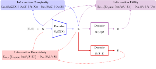
(a)

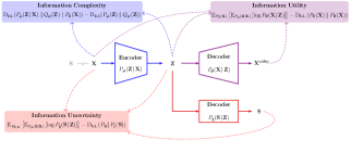
(b)

Figure 8: Block diagram of the DVCLUB associated with $(\text{P3})$ in the (a) supervised setup and (b) unsupervised setup.

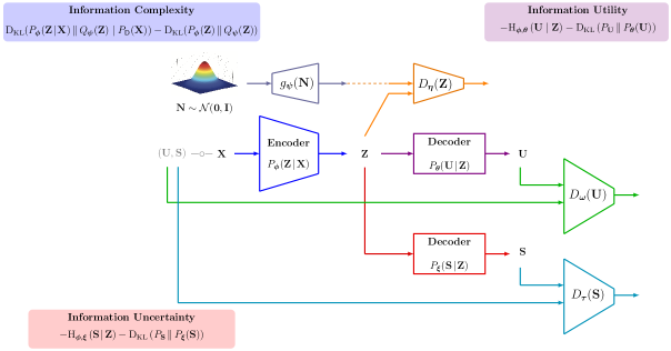
Figure 9: Supervised DVCLUB training architecture: considering the lower bound of information leakage.

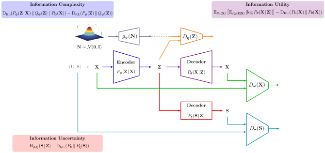
Figure 10: Unsupervised DVCLUB training architecture: considering the lower bound of information leakage.

7.2 Colored-MNIST Experiments

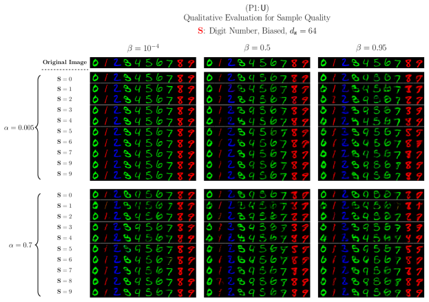
Figure 19: Qualitative evaluation for sample quality at the inferential adversary for unsupervised CLUB model ($\text{P1}\!\!:\!\mathsf{U}$) on Colored MNIST, setting $d_{\mathbf{z}}=64$, keeping the same setup as considered in Fig. 18.

The experiments on colored-MNIST dataset are depicted in this subsection. In order to study the impact of possible biases in the distribution of $\mathbf{S}$, we consider two scenarios for a digit color. In the uniform scenario the digits are randomly colored with the probabilities $P_{S}(\mathsf{Red})=P_{S}(\mathsf{Green})=P_{S}(\mathsf{Blue})=\frac{1}{3}$, while in the biased scenario the digits are randomly colored with the probabilities $P_{S}(\mathsf{Red})=\frac{1}{2}$, $P_{S}(\mathsf{Green})=\frac{1}{6}$, $P_{S}(\mathsf{Blue})=\frac{1}{3}$, and set $Q_{\bm{\psi}}\!\left(\mathbf{Z}\right)=\mathcal{N}\!\left(\bm{0},\mathbf{I}_{d}\right)$. The recognition accuracy of the utility attribute for the supervised CLUB model ($\text{P1}\!\!:\!\mathsf{S}$) is depicted in Fig. 11. The estimated information leakage for CLUB models (P1) and (P3) are depicted in Fig. 12 and Fig. 13, respectively, for the supervised and unsupervised setup. Fig. 14 depicts estimated information utility for the CLUB models ($\text{P1}\!\!:\!\mathsf{S}$) and ($\text{P3}\!\!:\!\mathsf{S}$). The MSE results of utility data $\mathbf{U}\equiv\mathbf{X}$ for the unsupervised scenarios ($\text{P1}\!\!:\!\mathsf{U}$) and ($\text{P3}\!\!:\!\mathsf{U}$), are depicted in Fig. 15. We provide a qualitative evaluation for sample quality at the inferential adversary for different CLUB models in Fig. 16, Fig. 17, Fig. 18, and Fig. 19. The training details and network architectures are provided in Appendix. A and Appendix B.

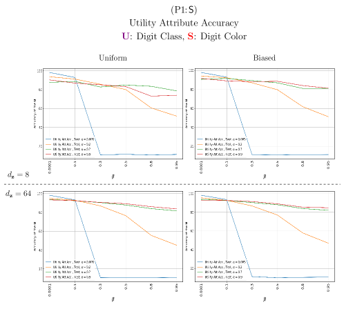
Figure 11: Recognition accuracy of the utility attribute $\mathbf{U}$ for supervised CLUB model ($\text{P1}\!\!:\!\mathsf{S}$) on ‘Test’ dataset of Colored-MNIST, considering $d_{\mathbf{z}}=8$ (First Row) and $d_{\mathbf{z}}=64$ (Second Row), setting $Q_{\bm{\psi}}\!\left(\mathbf{Z}\right)=\mathcal{N}\!\left(\bm{0},\mathbf{I}_{d_{\mathbf{z}}}\right)$, for different information complexity weights $\beta$ and information leakage weights $\alpha$. (Left Column): setting $P(\mathsf{Red})\!=\!P(\mathsf{Green})\!=\!P(\mathsf{Blue})\!=\!\frac{1}{3}$; (Right Column): setting $P(\mathsf{Red})\!=\!\frac{1}{2}$, $P(\mathsf{Green})\!=\!\frac{1}{6}$, $P(\mathsf{Blue})\!=\!\frac{1}{3}$.

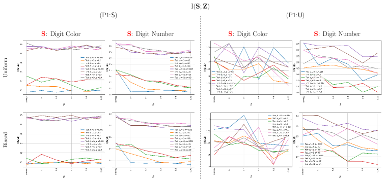
Figure 12: Estimated information leakage $\mathrm{I}(\mathbf{S};\mathbf{Z})$ on Colored-MNIST dataset using MINE, considering supervised and unsupervised scenarios ($\text{P1}\!\!:\!\mathsf{S}$) (Left Panel) and ($\text{P1}\!\!:\!\mathsf{U}$) (Right Panel), respectively, for $d_{\mathrm{z}}\in\{8,64\}$. (First Row): setting $P(\mathsf{Red})\!=\!P(\mathsf{Green})\!=\!P(\mathsf{Blue})\!=\!\frac{1}{3}$; (Second Row): setting $P(\mathsf{Red})\!=\!\frac{1}{2}$, $P(\mathsf{Green})\!=\!\frac{1}{6}$, $P(\mathsf{Blue})\!=\!\frac{1}{3}$.

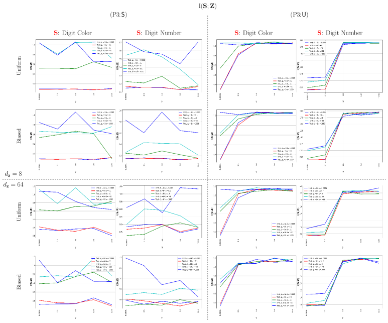
Figure 13: Estimated information leakage $\mathrm{I}(\mathbf{S};\mathbf{Z})$ on Colored-MNIST dataset using MINE, considering supervised and unsupervised scenarios ($\text{P3}\!\!:\!\mathsf{S}$) (Left Panel) and ($\text{P3}\!\!:\!\mathsf{U}$) (Right Panel), respectively, for $d_{\mathrm{z}}=8$ (Up Panel) and $d_{\mathrm{z}}=64$ (Down Panel). In each horizontal panel, (First Row): setting $P(\mathsf{Red})\!=\!P(\mathsf{Green})\!=\!P(\mathsf{Blue})\!=\!\frac{1}{3}$; (Second Row): setting $P(\mathsf{Red})\!=\!\frac{1}{2}$, $P(\mathsf{Green})\!=\!\frac{1}{6}$, $P(\mathsf{Blue})\!=\!\frac{1}{3}$.

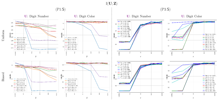
Figure 14: Estimated information utility $\mathrm{I}(\mathbf{U};\mathbf{Z})$ on Colored-MNIST dataset using MINE, considering supervised scenarios ($\text{P1}\!\!:\!\mathsf{S}$) (Left Panel) and ($\text{P3}\!\!:\!\mathsf{S}$) (Right Panel), for $d_{\mathrm{z}}\in\{8,64\}$. (First Row): setting $P(\mathsf{Red})\!=\!P(\mathsf{Green})\!=\!P(\mathsf{Blue})\!=\!\frac{1}{3}$; (Second Row): setting $P(\mathsf{Red})\!=\!\frac{1}{2}$, $P(\mathsf{Green})\!=\!\frac{1}{6}$, $P(\mathsf{Blue})\!=\!\frac{1}{3}$.

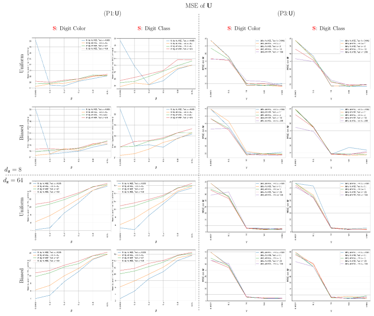
Figure 15: Mean Square Error of utility data $\mathbf{U}\equiv\mathbf{X}$ on Colored-MNIST dataset, considering unsupervised scenarios ($\text{P1}\!\!:\!\mathsf{U}$) (Left Panel) and ($\text{P3}\!\!:\!\mathsf{U}$) (Right Panel), for $d_{\mathrm{z}}=8$ (Up Panel) and $d_{\mathrm{z}}=64$ (Down Panel). In each horizontal panel, (First Row): setting $P(\mathsf{Red})\!=\!P(\mathsf{Green})\!=\!P(\mathsf{Blue})\!=\!\frac{1}{3}$; (Second Row): setting $P(\mathsf{Red})\!=\!\frac{1}{2}$, $P(\mathsf{Green})\!=\!\frac{1}{6}$, $P(\mathsf{Blue})\!=\!\frac{1}{3}$.

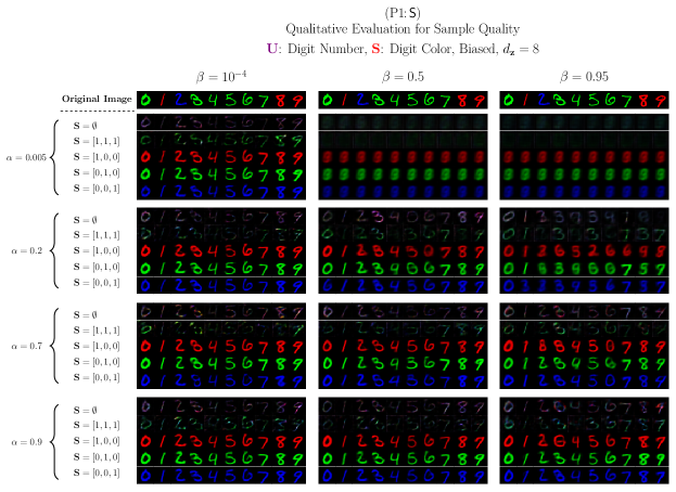
Figure 16: Qualitative evaluation for sample quality at the inferential adversary for supervised CLUB model ($\text{P1}\!\!:\!\mathsf{S}$) on Colored-MNIST, setting $d_{\mathbf{z}}=8$, $\mathbf{U}$: digit number, $\mathbf{S}$: digit color, $P_{S}(\mathsf{Red})=\frac{1}{2}$, $P_{S}(\mathsf{Green})=\frac{1}{6}$, $P_{S}(\mathsf{Blue})=\frac{1}{3}$, and $Q_{\bm{\psi}}\!\left(\mathbf{Z}\right)=\mathcal{N}\!\left(\bm{0},\mathbf{I}_{d}\right)$, for different trade-offs between $\beta$ and $\alpha$. From left to right: increasing information complexity weight $\beta$. From top to down: increasing information leakage weight $\alpha$. Five scenarios are considered to investigate the adversary’s beliefs about sensitive attribute $\mathbf{S}$. $\mathbf{S}=\emptyset$ corresponds to the case in which the adversary recovers $\mathbf{X}$ without any assumption on the digit color; $\mathbf{S}=\left[1,1,1\right]$ corresponds to a possible, probably meaningless, adversary’s belief about sensitive attribute to infer $\mathbf{S}$ from reconstructed $\mathbf{X}$; $\mathbf{S}=\left[1,0,0\right]$, $\mathbf{S}=\left[0,1,0\right]$, and $\mathbf{S}=\left[0,0,1\right]$ correspond to different adversary’s beliefs about sensitive attribute, i.e., the digit color, associated with $\mathsf{Red}$, $\mathsf{Green}$ and $\mathsf{Blue}$ colors, respectively. The results show that the adversary cannot revise his belief about $\mathbf{S}$.

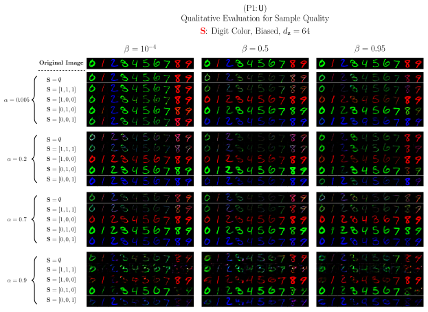
Figure 17: Qualitative evaluation for sample quality at the inferential adversary for supervised CLUB model ($\text{P1}\!\!:\!\mathsf{U}$) on Colored-MNIST, setting $d_{\mathbf{z}}=64$, keeping the same setup as considered in Fig. 16.

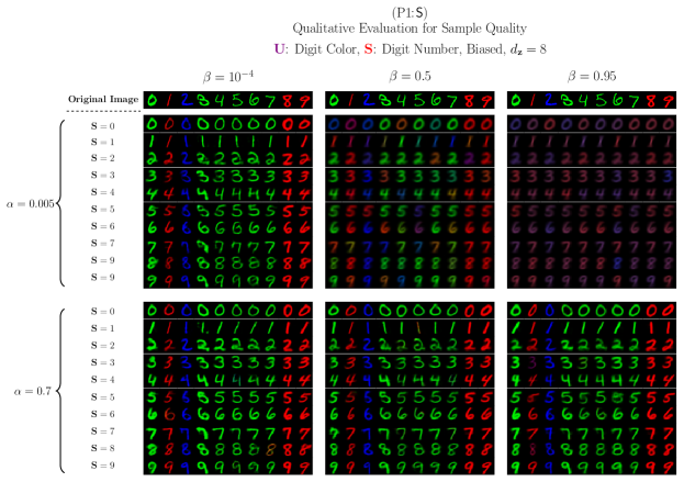
Figure 18: Qualitative evaluation for sample quality at the inferential adversary for supervised CLUB model ($\text{P1}\!\!:\!\mathsf{S}$) on Colored-MNIST, setting $d_{\mathbf{z}}=8$, $\mathbf{U}$: digit color, $\mathbf{S}$: digit number, $P_{U}(\mathsf{Red})=\frac{1}{2}$, $P_{U}(\mathsf{Green})=\frac{1}{6}$, $P_{U}(\mathsf{Blue})=\frac{1}{3}$, and $Q_{\bm{\psi}}\!\left(\mathbf{Z}\right)=\mathcal{N}\!\left(\bm{0},\mathbf{I}_{d}\right)$, for different trade-offs between $\beta$ and $\alpha$. From left to right: increasing information complexity weight $\beta$. From top to down: increasing information leakage weight $\alpha$. Ten scenarios are considered to investigate the adversary’s beliefs about sensitive attribute $\mathbf{S}$. Each scenario corresponds to the case in which the adversary recovers $\mathbf{X}$ with a assumption on the digit number. The results show that the adversary cannot revise his belief about $\mathbf{S}$.

7.3 CelebA Experiments

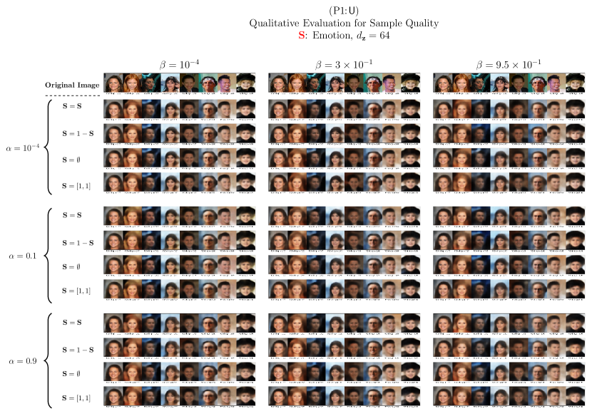
Figure 28: Qualitative evaluation for sample quality at the inferential adversary for unsupervised CLUB model ($\text{P1}\!\!:\!\mathsf{U}$) on CelebA, setting $\mathbf{S}$: Emotion, and keeping the same setup as considered in Fig. 27. Emotion probabilities are computed and depicted under each image.

The experiments on CelebA dataset are depicted in this subsection. The recognition accuracy of the utility attribute for the supervised CLUB models ($\text{P1}\!\!:\!\mathsf{S}$) and ($\text{P3}\!\!:\!\mathsf{S}$) are depicted in Fig. 20 and Fig. 21, respectively. The recognition accuracy of the sensitive attribute for the unsupervised CLUB models ($\text{P1}\!\!:\!\mathsf{U}$) and ($\text{P3}\!\!:\!\mathsf{U}$) is depicted in Fig. 22. The estimated information leakage for CLUB models (P1) and (P3) are depicted in Fig. 23 and Fig. 24, respectively, for the supervised and unsupervised setup. Fig. 25 depicts estimated information utility for the CLUB models ($\text{P1}\!\!:\!\mathsf{S}$) and ($\text{P3}\!\!:\!\mathsf{S}$). The MSE results of utility data $\mathbf{U}\equiv\mathbf{X}$ for the unsupervised scenarios ($\text{P1}\!\!:\!\mathsf{U}$) and ($\text{P3}\!\!:\!\mathsf{U}$), are depicted in Fig. 26. We provide a qualitative evaluation for sample quality at the inferential adversary for different CLUB models in Fig. 27 and Fig. 28. The training details and network architectures are provided in Appendix. A and Appendix B.

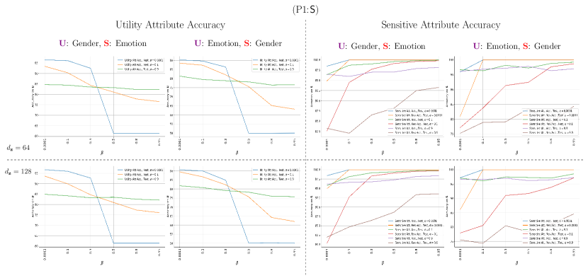
Figure 20: Recognition accuracy of the utility attribute $\mathbf{U}$ (Left Panel) and sensitive attribute $\mathbf{S}$ (Right Panel) for supervised CLUB model ($\text{P1}\!\!:\!\mathsf{S}$) on ‘Test’ dataset of CelebA, considering $d_{\mathbf{z}}=64$ (First Row) and $d_{\mathbf{z}}=128$ (Second Row), setting $Q_{\bm{\psi}}\!\left(\mathbf{Z}\right)=\mathcal{N}\!\left(\bm{0},\mathbf{I}_{d_{\mathbf{z}}}\right)$, for different information complexity weights $\beta$ and information leakage weights $\alpha$. For each panel, (Left Column): utility task is gender recognition, sensitive attribute is emotion (smiling); (Right Column): utility task is emotion (smiling) recognition, sensitive attribute is gender.

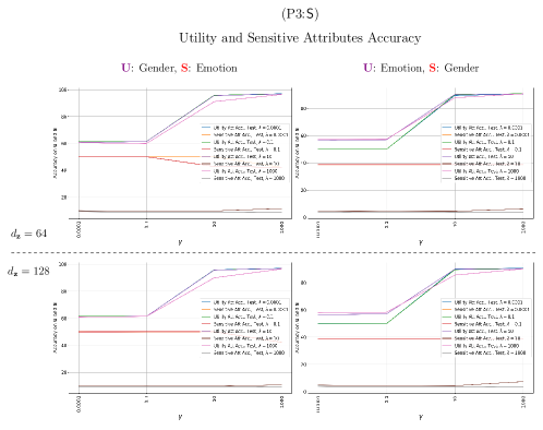
Figure 21: Recognition accuracy of the utility attribute $\mathbf{U}$ and sensitive attribute $\mathbf{S}$ for supervised CLUB model ($\text{P3}\!\!:\!\mathsf{S}$) on ‘Test’ dataset of CelebA, considering $d_{\mathbf{z}}=64$ (First Row) and $d_{\mathbf{z}}=128$ (Second Row), setting $Q_{\bm{\psi}}\!\left(\mathbf{Z}\right)=\mathcal{N}\!\left(\bm{0},\mathbf{I}_{d_{\mathbf{z}}}\right)$, for different information utility weights $\gamma$ and information leakage weights $\lambda$. (Left Column): utility task is gender recognition, sensitive attribute is emotion (smiling); (Right Column): utility task is emotion (smiling) recognition, sensitive attribute is gender.

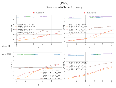
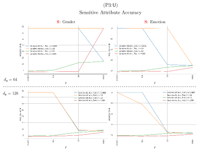
Figure 22: Recognition accuracy of the sensitive attribute $\mathbf{S}$ for unsupervised CLUB models ($\text{P1}\!\!:\!\mathsf{U}$) (Left Panel) and ($\text{P3}\!\!:\!\mathsf{U}$) (Right Panel) on ‘Test’ dataset of CelebA, considering $d_{\mathbf{z}}=64$ (First Row) and $d_{\mathbf{z}}=128$ (Second Row), setting $Q_{\bm{\psi}}\!\left(\mathbf{Z}\right)=\mathcal{N}\!\left(\bm{0},\mathbf{I}_{d_{\mathbf{z}}}\right)$; for different information complexity weights $\beta$ and information leakage weights $\alpha$ in ($\text{P1}\!\!:\!\mathsf{U}$), and for different information utility weights $\gamma$ and information leakage weights $\lambda$ in ($\text{P3}\!\!:\!\mathsf{U}$). For each panel, (Left Column): sensitive attribute is gender; (Right Column): sensitive attribute is emotion (smiling).

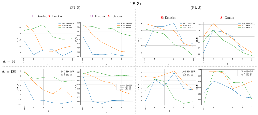
Figure 23: Estimated information leakage $\mathrm{I}(\mathbf{S};\mathbf{Z})$ for CLUB models ($\text{P1}\!\!:\!\mathsf{S}$) (Left Panel) and ($\text{P1}\!\!:\!\mathsf{U}$) (Right Panel) on ‘Test’ dataset of CelebA using MINE, considering $d_{\mathbf{z}}=64$ (First Row) and $d_{\mathbf{z}}=128$ (Second Row), setting $Q_{\bm{\psi}}\!\left(\mathbf{Z}\right)=\mathcal{N}\!\left(\bm{0},\mathbf{I}_{d_{\mathbf{z}}}\right)$, for different information complexity weights $\beta$ and information leakage weights $\alpha$.

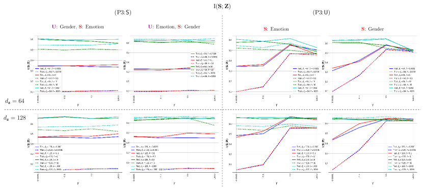
Figure 24: Estimated information leakage $\mathrm{I}(\mathbf{S};\mathbf{Z})$ for CLUB models ($\text{P3}\!\!:\!\mathsf{S}$) (Left Panel) and ($\text{P3}\!\!:\!\mathsf{U}$) (Right Panel) on ‘Test’ and ‘Train’ datasets of CelebA using MINE, considering $d_{\mathbf{z}}=64$ (First Row) and $d_{\mathbf{z}}=128$ (Second Row), setting $Q_{\bm{\psi}}\!\left(\mathbf{Z}\right)=\mathcal{N}\!\left(\bm{0},\mathbf{I}_{d_{\mathbf{z}}}\right)$, for different information utility weights $\gamma$ and information leakage weights $\lambda$.

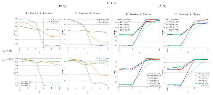
Figure 25: Estimated information utility $\mathrm{I}(\mathbf{U};\mathbf{Z})$ for supervised CLUB models ($\text{P1}\!\!:\!\mathsf{S}$) (Left Panel) and ($\text{P3}\!\!:\!\mathsf{S}$) (Right Panel) on ‘Test’ and ‘Train’ datasets of CelebA using MINE, considering $d_{\mathbf{z}}=64$ (First Row) and $d_{\mathbf{z}}=128$ (Second Row), setting $Q_{\bm{\psi}}\!\left(\mathbf{Z}\right)=\mathcal{N}\!\left(\bm{0},\mathbf{I}_{d_{\mathbf{z}}}\right)$, for different information complexity weights $\beta$ and information leakage weights $\alpha$ in ($\text{P1}\!\!:\!\mathsf{S}$), and for different information utility weights $\gamma$ and information leakage weights $\lambda$ in ($\text{P3}\!\!:\!\mathsf{S}$).

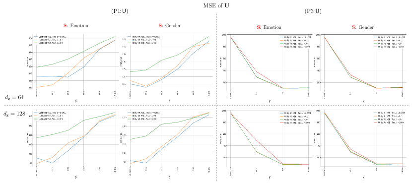
Figure 26: Mean Square Error (MSE) of reconstructed $\mathbf{U}\equiv\mathbf{X}$ for unsupervised CLUB models ($\text{P1}\!\!:\!\mathsf{U}$) (Left Panel) and ($\text{P3}\!\!:\!\mathsf{U}$) (Right Panel) on ‘Test’ dataset of CelebA, considering $d_{\mathbf{z}}=64$ (First Row) and $d_{\mathbf{z}}=128$ (Second Row), setting $Q_{\bm{\psi}}\!\left(\mathbf{Z}\right)=\mathcal{N}\!\left(\bm{0},\mathbf{I}_{d_{\mathbf{z}}}\right)$, for different information complexity weights $\beta$ and information leakage weights $\alpha$ in ($\text{P1}\!\!:\!\mathsf{U}$), and for different information utility weights $\gamma$ and information leakage weights $\lambda$ in ($\text{P3}\!\!:\!\mathsf{U}$).

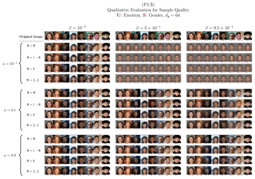
Figure 27: Qualitative evaluation for sample quality at the inferential adversary for supervised CLUB model ($\text{P1}\!\!:\!\mathsf{S}$) on CelebA, setting $d_{\mathbf{z}}=64$, $\mathbf{U}$: Emotion, $\mathbf{S}$: Gender, $Q_{\bm{\psi}}\!\left(\mathbf{Z}\right)=\mathcal{N}\!\left(\bm{0},\mathbf{I}_{d}\right)$, for different trade-offs between $\beta$ and $\alpha$. From left to right: increasing information complexity weight $\beta$. From top to down: increasing information uncertainly weight $\alpha$. Four scenarios are considered to investigate the adversary’s beliefs about sensitive attribute $\mathbf{S}$. $\mathbf{S}=\mathbf{S}$ corresponds to the case in which the adversary recovers $\mathbf{X}$ when his belief coincides with the original $\mathbf{S}$ (i.e., $\mathbf{S}=\left[1,0\right]$ for man, and $\mathbf{S}=\left[0,1\right]$ for woman); $\mathbf{S}=1-\mathbf{S}$ corresponds to the case in which the adversary recovers $\mathbf{X}$ when his belief coincides with the inverse of original $\mathbf{S}$; $\mathbf{S}=\emptyset$ corresponds to the case in which the adversary recovers $\mathbf{X}$ without any assumption on the sensitive attribute $\mathbf{S}$; $\mathbf{S}=\left[1,1\right]$ correspond to a possible, probably meaningless, adversary’s belief about sensitive attribute, to infer the sensitive attribute $\mathbf{S}$ from reconstructed $\mathbf{X}$. Gender probabilities are computed and depicted under each image. These probabilities show how accurately an adversary can revise his belief about $\mathbf{S}$, at different information leakage weights $\alpha$ and information complexity weights $\beta$.

8 Conclusion

We proposed a general family of optimization problems that unified and generalized most of the state-of-the-art information-theoretic privacy models. We first addressed obfuscation and utility measures under logarithmic loss, and then expressed the concept of relevant information from information-theoretic, statistical, and measure-theoretic perspectives. We then introduced and characterized the CLUB optimization problem and established a variational lower bound to optimize the associated CLUB Lagrangian functional. We constructed the DVCLUB models by employing neural networks to parameterize variational approximations of the information complexity, information leakage, and information utility quantities. We also proposed alternating block coordinate descent training algorithms associated with the proposed DVCLUB models. The DVCLUB model sheds light on the connections between information theory and generative models, deep compression models, as well as, fair machine learning models. In addition, this unifying perspective allows us to relate the CLUB model to several information-theoretic coding problems. Constructing an $\mathrm{I}$-measure, consistent with Shannon’s information measures, we geometrically represent the relationship among Shannon’s information measures in state-of-the-art bottleneck problems, interpreting the differences in their objectives. Although the CLUB model is formulated using Shannon’s mutual information, which leads us to self-consistent equations, one can use other information measures with different operational meanings.

tablesection figuresection

Appendix A Training Details

All of the experiments in the study were carried out in the following order:

1.01 Warm-up Phase

We utilize the warm-up phase before running training Algorithms 1,2,3,4 for all experiments. In the warm-up phase, we pre-trained encoder $\left(f_{\bm{\phi}}\right)$ and utility-decoder $\left(g_{\bm{\theta}}\right)$ together for a few epochs via backpropagation with the Adam optimizer [200]. We found out the warm-up stage was helpful in method convergence speed. Therefore, we initialize the encoder and the utility-decoder weights with the obtained values rather than random or zero initialization. For each experiment, the hyper-parameters of the learning algorithm in this phase are depicted in TABLE I.

Experiment Dataset	Learning Rate	Max Iteration	Batch Size
Colored-MNIST	0.001	50	1024
(both version)
CelebA	0.005	50	1024

TABLE I: Models’ hyper-parameters in the Warm-Up phase for the experiments.

1.02 Main Block-wised Training Phase

In contrast to most neural network models that only have one forward step and a backward step in each epoch to update all network weights, each of our learning algorithms consists of several blocks in which forward and backward steps have been done on different paths. The model’s parameters update based on the corresponding path.

Since it was not possible for us to use the default model training function of the Keras API, we implement All six training Algorithms 1,2,3,4 from scratch in Tensorflow. It is important to remember that we initialize all parameters to zero except for the $\left(\bm{\phi},\bm{\theta}\right)$ values acquired in the previous stage. Furthermore, we set the learning rate of the block (1) in all Algorithms to five times larger than other blocks. The hyper-parameters of models for each experiment are shown in TABLE II.

Experiment Dataset	Learning Rate	Max Iteration	Batch Size
	[blocks (2)-(5)]
Colored-MNIST	0.0001	500	2048
(both version)
CelebA	0.00001	500	1024

TABLE II: Models’ hyper-parameters in the main phase for the experiments.

Appendix B Network Architecture

2.01 Colored-MNIST

In the Colored-MNIST experiment, we consider two setups for data utility and information leakage evaluation. In the first scenario, we set the utility data to the class label of the input image and consider the color of the input image as sensitive data, and for the second one, we did vice versa. It is worth mentioning both balanced and unbalanced Colored-MNIST datasets are applied with the same architecture. The architecture of networks is given in Table III and IV.

Encoder ($f_{\bm{\phi}}$) - Both Setups

Input  $\mathbf{x}\in\mathbb{R}^{28\times 28\times 3}$ Color Image

Conv(64,5,2), BN, LeakyReLU

Conv(128,5,2), BN, LeakyReLU

Flatten

FC($d_{z}\times 4$), BN, Tanh

$\mu$= FC($d_{z}$), $\sigma$= FC($d_{z}$)

$z$=SamplingWithReparameterizationTrick[$\mu$,$\sigma$]

Utility Decoder ($g_{\bm{\theta}}$) - Supervised Setup

Input  $\mathbf{z}\in\mathbb{R}^{d_{z}}$ Code

FC($d_{z}\times 4$), BN, LeakyReLU

FC($|\mathcal{U}|$), SOFTMAX

Utility Decoder ($g_{\bm{\theta}}$) - Unsupervised Setup

Input  $\mathbf{z}\in\mathbb{R}^{d_{\mathrm{z}}}$ Code

FC($6272$), BN, LeakyReLU

Reshape($(7,7,128)$)

DeConv($64,5,2$), BN, LeakyReLU

DeConv($3,5,2$), Sigmoid

Uncertainty Decoder ($g_{\bm{\varphi}}$)

Input  $\mathbf{z}\in\mathbb{R}^{d_{\mathrm{z}}}$ Code

FC($6272$), BN, LeakyReLU

Reshape($(7,7,128)$)

DeConv($64,5,2$), BN, LeakyReLU

DeConv($3,5,2$), Sigmoid

Uncertainty Decoder ($g_{\bm{\xi}}$)

Input  $\mathbf{z}\in\mathbb{R}^{d_{\mathrm{z}}}$ Code, $\mathbf{s}\in\mathbb{R}^{|\mathcal{U}|}$

$\mathbf{zs}$ = concatenate($\mathbf{z},\mathbf{s}$)

FC($2\times 2\times 256$), BN, LeakyReLU

Reshape($(256,2,2)$)

DeConv($(128,3,2)$), BN, LeakyReLU

DeConv($(64,3,2)$), BN, LeakyReLU

DeConv($(32,3,2)$), BN, LeakyReLU

DeConv($(16,3,2)$), BN, LeakyReLU

DeConv($(8,3,2)$), BN, LeakyReLU

Conv($3,3,2$), Sigmoid

Prior Distribution Generator ($g_{\bm{\psi}}$) - Both Setups

Input  Sample Noise$\sim\mathcal{N}\!\left(\bm{0},\mathbf{I}\right)$

FC($100$), BN, LeakyReLU

FC($100$), BN, LeakyReLU

FC($|d_{z}|$), Sigmoid

TABLE III: The encoders and decoders architecture for the Colored-MNIST experiments.

Latent Space Discriminator ($D_{\bm{\eta}}$)

Input  $\mathbf{z}\in\mathbb{R}^{d_{z}}$ Code

FC($128$), BN, LeakyReLU

FC($64$), BN, LeakyReLU

FC($1$), Sigmoid

Utility Attribute Class Discriminator ($D_{\bm{\omega}}$)

Input  $\mathbf{u}\in\mathbb{R}^{|\mathcal{U}|}$

FC($|\mathcal{U}|\times 8$), BN, LeakyReLU

FC($|\mathcal{U}|\times 8$), BN, LeakyReLU

FC($1$), Sigmoid

Visible Space Discriminator ($D_{\bm{\omega}}$)

Input  $\mathbf{\widehat{x}}\in\mathbb{R}^{28\times 28\times 3}$  Color Image

Conv($32,3,2$), BN, LeakyReLU

Conv($64,3,2$), BN, LeakyReLU

Conv($128,3,2$), BN, LeakyReLU

Flatten

FC($128$), BN, LeakyReLU

FC($1$), Sigmoid

TABLE IV: The discriminators architecture details for the Colored-MNIST experiments.

2.02 Mutual Information Estimation

For all experiments in this paper, we report estimation of MI between the released representation and sensitive attribute, i.e., $\mathrm{I}\left(\mathbf{S};\mathbf{Z}\right)$, as well as the MI between the released representation and utility attribute, i.e., $\mathrm{I}\left(\mathbf{U};\mathbf{Z}\right)$. To approximate mutual information, we employed the MINE model [201]. The architecture of the model is depicted in V. Note that MINE’s network for estimating $\mathrm{I}\left(\mathbf{S};\mathbf{Z}\right)$ has the same architecture as shown in Table V.

MINE    $\mathrm{I}\left(\mathbf{U};\mathbf{Z}\right)$

Input  $\mathbf{z}\in\mathbb{R}^{d_{z}}$ Code; $\mathbf{u}\in\mathbb{R}^{|\mathcal{U}|}$

x = Concatenate([z, u])

FC(100), ELU

FC(100), ELU

FC(100), ELU

FC(1)

TABLE V: The architecture of MINE network for mutual information estimation.

2.03 CelebA

In this experiment, we considered two scenarios for data utility and sensitive attributes. These setups are shown in Table VI. Note that all of the utility and sensitive attributes are binary data. The architecture of networks is given in Table VII.

Scenario Number	Utility Attribute	Sensitive Attribute
1	Gender	Smiling
2	Smiling	Gender

TABLE VI: The considered scenarios for the CelebA experiments.

Encoder $f_{\bm{\phi}}$ - Both Setups

Input  $\mathbf{x}\in\mathbb{R}^{64\times 64\times 3}$ Color Image

Conv(64,5,2), BN, LeakyReLU

Conv(128,5,2), BN, LeakyReLU

Flatten

FC($d_{z}\times 4$), BN, Tanh

$\mu$= FC($d_{z}$), $\sigma$= FC($d_{z}$)

$z$=SamplingWithReparameterizationTrick[$\mu$,$\sigma$]

Utility Decoder ($g_{\bm{\theta}}$) - Supervised Setups

Input  $\mathbf{z}\in\mathbb{R}^{d_{z}}$ Code

FC($d_{z}\times 4$), BN, LeakyReLU

FC($|\mathcal{U}|$), SOFTMAX

Utility Decoder ($g_{\bm{\theta}}$) - Unsupervised Setups

Input  $\mathbf{z}\in\mathbb{R}^{d_{\mathrm{z}}}$ Code

FC($7\times 7\times 128$), BN, LeakyReLU

Reshape($(7,7,128)$)

DeConv($64,5,2$), BN, LeakyReLU

DeConv($3,5,2$), Sigmoid

Uncertainty Decoder ($g_{\bm{\varphi}}$) - Supervised Setups

Input  $\mathbf{z}\in\mathbb{R}^{d_{\mathrm{z}}}$ Code, $\mathbf{s}\in\mathbb{R}^{|\mathcal{U}|}$

$\mathbf{zs}$ = concatenate($\mathbf{z},\mathbf{s}$)

FC($7\times 7\times 128$), BN, LeakyReLU

Reshape($(128,7,7)$), BN, LeakyReLU

DeConv($(64,5,2)$), BN, LeakyReLU

DeConv($(3,5,2)$), Sigmoid

Uncertainty Decoder ($g_{\bm{\xi}}$)

Input  $\mathbf{z}\in\mathbb{R}^{d_{\mathrm{z}}}$ Code

FC($d_{\mathrm{z}}\times 4$), BN, LeakyReLU

FC($|\mathcal{S}|$), Softmax

Prior Distribution Generator ($g_{\bm{\psi}}$)

Input  Sample Noise$\sim\mathcal{N}\!\left(\bm{0},\mathbf{I}\right)$

FC($100$), BN, LeakyReLU

FC($100$), BN, LeakyReLU

FC($|d_{z}|$), Sigmoid

TABLE VII: The encoders and decoders architecture for the CelebA experiments.

Latent Space Discriminator ($D_{\bm{\eta}}$)

Input  $\mathbf{z}\in\mathbb{R}^{d_{z}}$ Code

FC($512$), BN, LeakyReLU

FC($128$), BN, LeakyReLU

FC($1$), Sigmoid

Utility Attribute Class Discriminator ($D_{\bm{\omega}}$)

Input  $\mathbf{u}\in\mathbb{R}^{|\mathcal{U}|}$

FC($|\mathcal{U}|\times 4$), BN, LeakyReLU

FC($|\mathcal{U}|\times 4$), BN, LeakyReLU

FC($1$), Sigmoid

Visible Space Discriminator ($D_{\bm{\omega}}$)

Input  $\mathbf{x}\in\mathbb{R}^{64\times 64\times 3}$ Color Image

Conv(32,3,2), BN, LeakyReLU

Conv(64,3,2), BN, LeakyReLU

Conv(128,3,2), BN, LeakyReLU

Flatten

FC($128$), BN, LeakyReLU

FC($1$), Sigmoid

TABLE VIII: The discriminators architecture for the CelebA experiments.

Appendix C Implementation Overview

Considering Algorithm 1 and Algorithm 2, the main loop consists of ‘five’ blocks where only some networks are used in the forward phase, and mostly one of them would update their parameters via back propagation in each block. Therefore, we shattered the model into four sub-modules in the training stage for simplicity and performance. For the sake of visualization, we demonstrate a collection of sub-networks of the CLUB models in Fig. 29, Fig. 30, Fig. 31, and Fig. 32.

During training, all of the sub-module (d) parameters, call the "auto-encoder part" would update with BP after each forward step. For the sub-modules (a), (b), and (c), only the parameters of one network are updated when the corresponding error function values back-propagate, and we freeze the other network parameters in the sub-module. For example, block (3) of Algorithm 1 is related to the (c) sub-module, but at the BP step, the latent space discriminator is frozen to prevent its parameters from updating.

It should be mentioned that during our experiments, we found out that before running our main algorithm, it is beneficial to pre-train the auto-encoder sub-module since we need to sample from the latent space, which uses in other parts of the main model during training. We justify this by mentioning that sampling meaningful data rather than random ones from latent variables from the beginning of learning helps the model to converge better and faster in comparison with starting one of our DVCLUB algorithms with a randomly initiated auto-encoder.

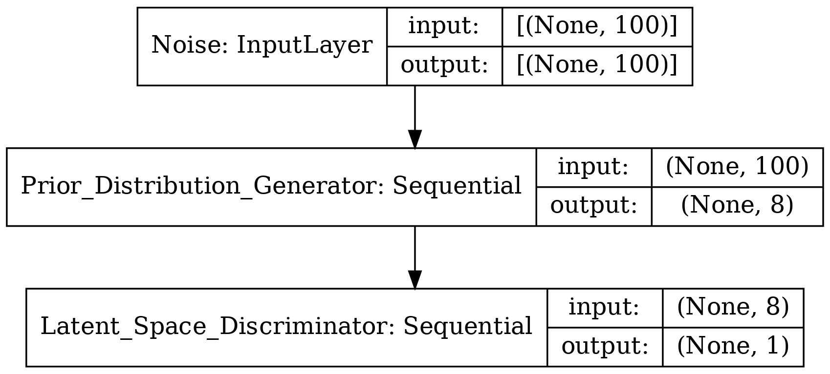
(a) Prior-Generator adjoint Latent-Space-Discriminator module

(b) Utility-Decoder adjoint Attribute-Class-Discriminator module

(c) Encoder adjoint Latent-Space-Discriminator module

(d) The auto-encoder module

Figure 29: All model modules for supervised CLUB algorithm associated with ($\text{P1}\!\!:\!\mathsf{S}$) on Colored-MNIST dataset, setting $\mathbf{U}$: Digit Color, $\mathbf{S}$: Digit Class. The encoder output is set to 8 neurons.

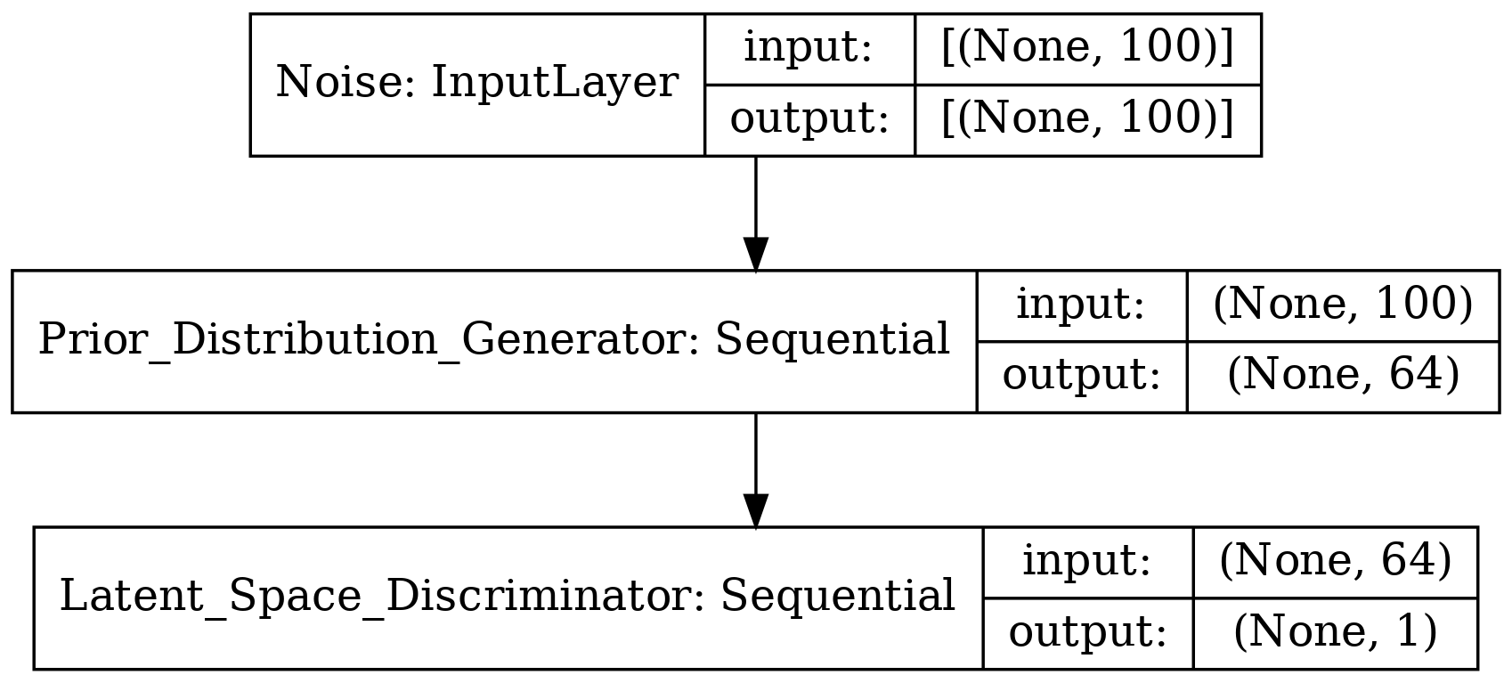
(a) Prior-Generator adjoint Latent-Space-Discriminator module

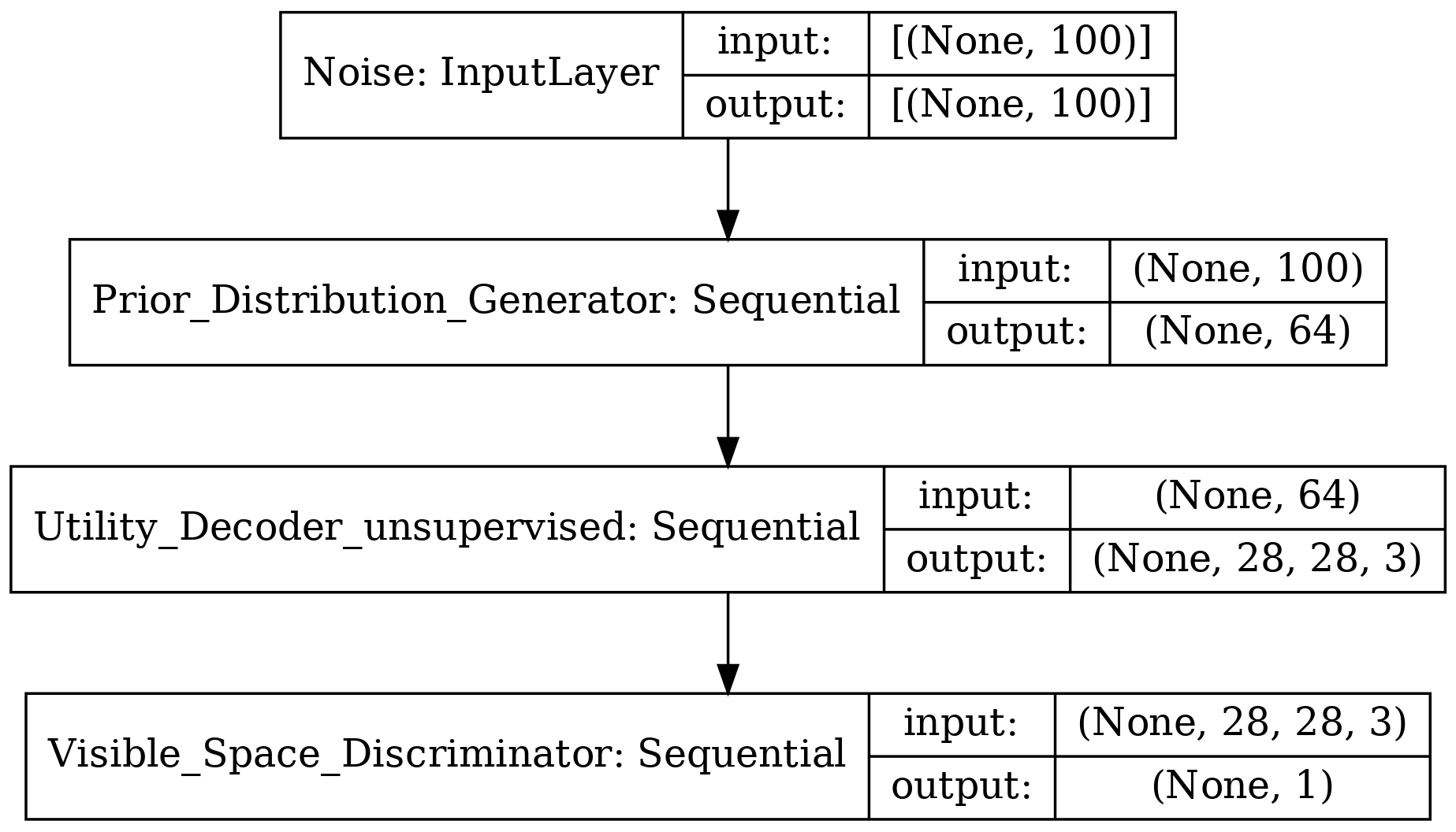
(b) Utility-Decoder adjoint Attribute-Class-Discriminator module

(c) Encoder adjoint Latent-Space-Discriminator module

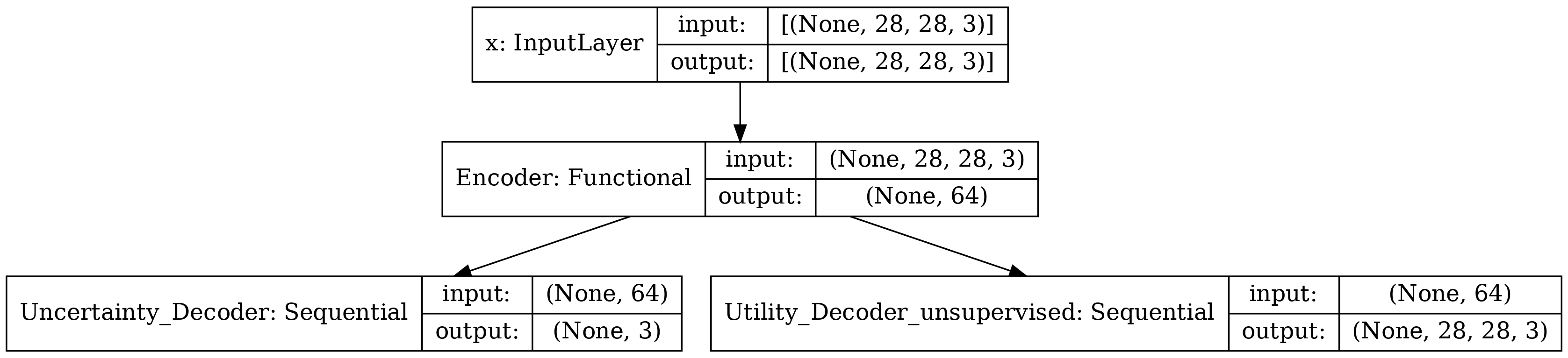
(d) The auto-encoder module

Figure 30: All model modules for unsupervised CLUB algorithm associated with ($\text{P3}\!\!:\!\mathsf{U}$) on Colored-MNIST dataset, setting $\mathbf{U}$: Digit Class, $\mathbf{S}$: Digit Color. The encoder output is set to 64 neurons.

(a) Prior-Generator adjoint Latent-Space-Discriminator module

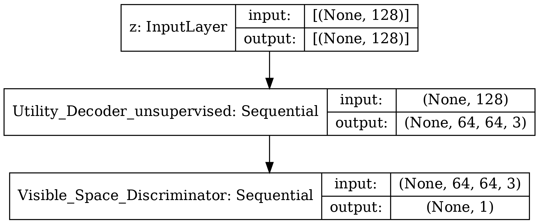
(b) Utility-Decoder adjoint Attribute-Class-Discriminator module

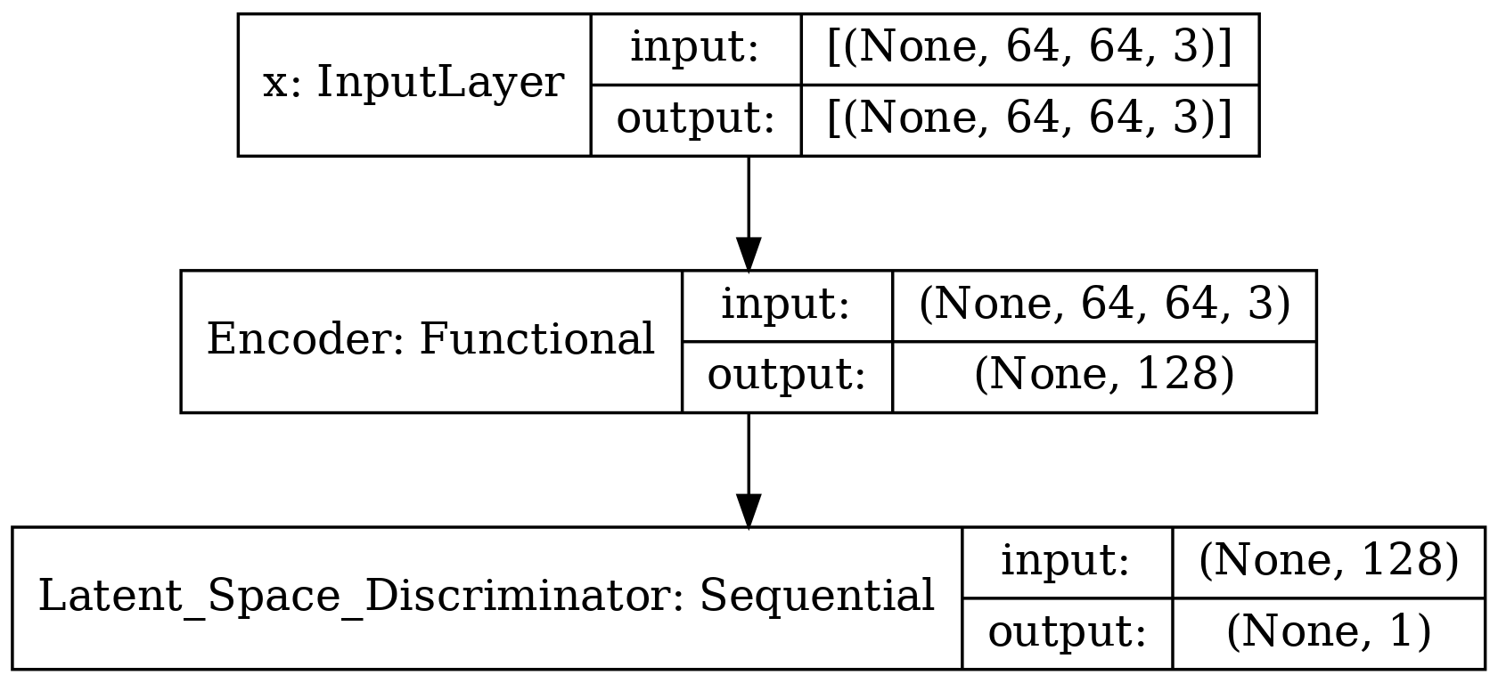
(c) Encoder adjoint Latent-Space-Discriminator module

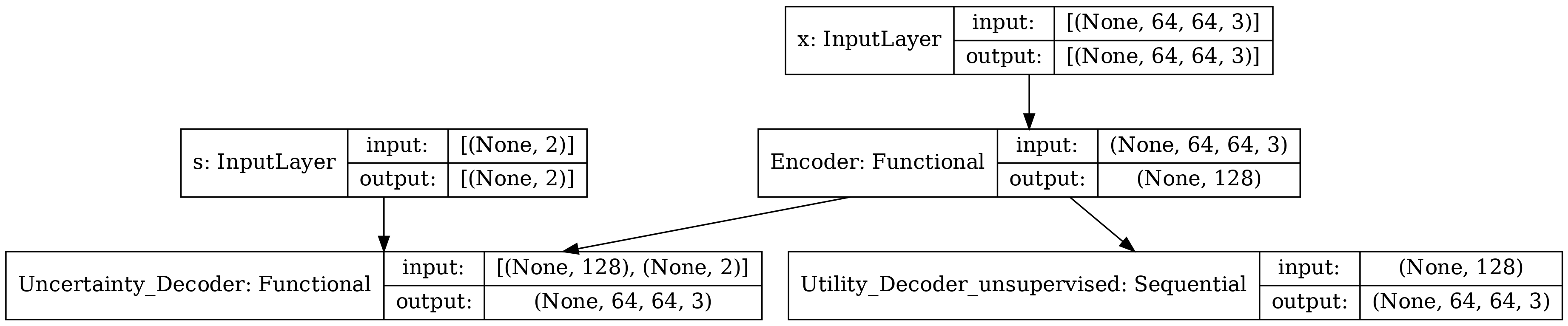
(d) The auto-encoder module

Figure 31: All model modules for unsupervised CLUB algorithm associated with ($\text{P1}\!\!:\!\mathsf{U}$) on CelebA dataset, setting $\mathbf{U}$: Gender, $\mathbf{S}$: Emotion. The encoder output is set to 128 neurons.

(a) Prior-Generator adjoint Latent-Space-Discriminator module

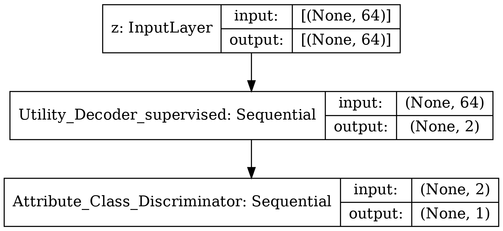
(b) Utility-Decoder adjoint Attribute-Class-Discriminator module

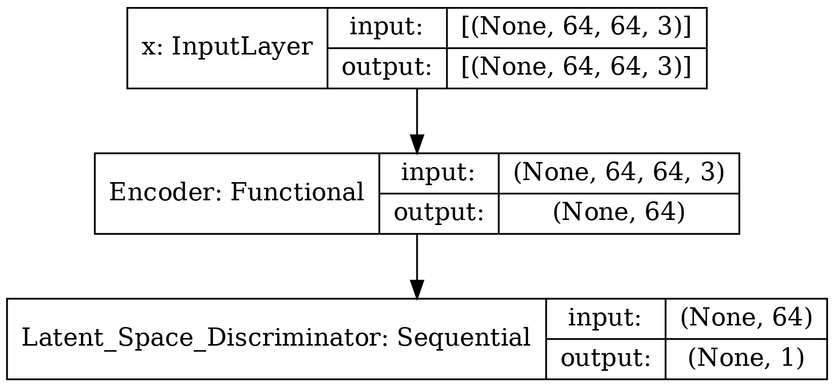
(c) Encoder adjoint Latent-Space-Discriminator module

(d) The auto-encoder module

Figure 32: All model modules for supervised CLUB algorithm associated with ($\text{P3}\!\!:\!\mathsf{S}$) on CelebA dataset, setting $\mathbf{U}$: Emotion, $\mathbf{S}$: Gender. The encoder output is set to 64 neurons.

Appendix D Supplementary Results

4.1 Supplementary Results of Colored-MNIST Experiments

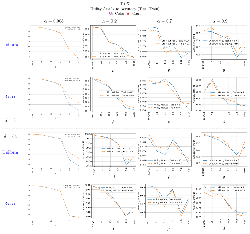
Figure 33: Recognition accuracy of the utility attribute $\mathbf{U}$ for supervised CLUB model ($\text{P1}\!\!:\!\mathsf{S}$) on ‘Test’ and ‘Train’ datasets of Colored-MNIST, considering $d_{\mathbf{z}}=8$ (Up Panel) and $d_{\mathbf{z}}=64$ (Down Panel), setting $Q_{\bm{\psi}}\!\left(\mathbf{Z}\right)=\mathcal{N}\!\left(\bm{0},\mathbf{I}_{d_{\mathbf{z}}}\right)$, for different information complexity weights $\beta$ and information leakage weights $\alpha$.

4.2 Supplementary Results of CelebA Experiments

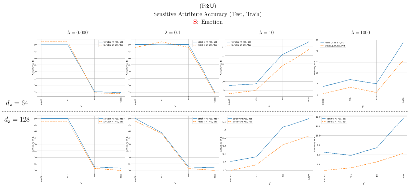
Figure 34: Recognition accuracy of the sensitive attribute $\mathbf{S}$ for unsupervised CLUB model ($\text{P3}\!\!:\!\mathsf{U}$) on ‘Test’ and ‘Train’ datasets of CelebA, considering $d_{\mathbf{z}}=64$ (First Row) and $d_{\mathbf{z}}=128$ (Second Row), setting $\mathbf{S}$: Emotion (smiling), $Q_{\bm{\psi}}\!\left(\mathbf{Z}\right)=\mathcal{N}\!\left(\bm{0},\mathbf{I}_{d_{\mathbf{z}}}\right)$, for different information utility weights $\gamma$ and information leakage weights $\lambda$.

Figure 35: Recognition accuracy of the sensitive attribute $\mathbf{S}$ for unsupervised CLUB model ($\text{P3}\!\!:\!\mathsf{U}$) on ‘Test’ and ‘Train’ datasets of CelebA, considering $d_{\mathbf{z}}=64$ (First Row) and $d_{\mathbf{z}}=128$ (Second Row), setting $\mathbf{S}$: Gender, $Q_{\bm{\psi}}\!\left(\mathbf{Z}\right)=\mathcal{N}\!\left(\bm{0},\mathbf{I}_{d_{\mathbf{z}}}\right)$, for different information utility weights $\gamma$ and information leakage weights $\lambda$.

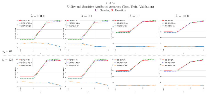
Figure 36: Recognition accuracy of the utility attribute $\mathbf{U}$ and sensitive attribute $\mathbf{S}$ for supervised CLUB model ($\text{P3}\!\!:\!\mathsf{S}$) on ‘Test’, ‘Train’ and ‘Validation’ datasets of CelebA, considering $d_{\mathbf{z}}=64$ (First Row) and $d_{\mathbf{z}}=128$ (Second Row), setting $\mathbf{U}$: Gender, $\mathbf{S}$: Emotion (smiling), $Q_{\bm{\psi}}\!\left(\mathbf{Z}\right)=\mathcal{N}\!\left(\bm{0},\mathbf{I}_{d_{\mathbf{z}}}\right)$, for different information utility weights $\gamma$ and information leakage weights $\lambda$.

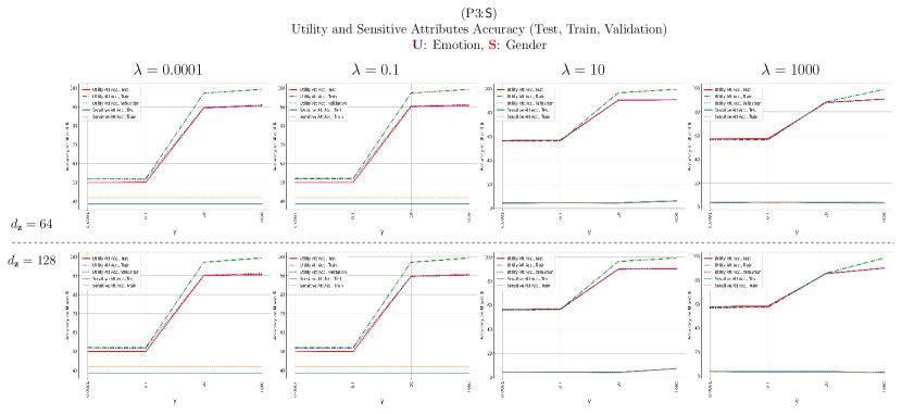
Figure 37: Recognition accuracy of the utility attribute $\mathbf{U}$ and sensitive attribute $\mathbf{S}$ for supervised CLUB model ($\text{P3}\!\!:\!\mathsf{S}$) on ‘Test’, ‘Train’ and ‘Validation’ datasets of CelebA, considering $d_{\mathbf{z}}=64$ (First Row) and $d_{\mathbf{z}}=128$ (Second Row), setting $\mathbf{U}$: Emotion (smiling), $\mathbf{S}$: Gender, $Q_{\bm{\psi}}\!\left(\mathbf{Z}\right)=\mathcal{N}\!\left(\bm{0},\mathbf{I}_{d_{\mathbf{z}}}\right)$, for different information utility weights $\gamma$ and information leakage weights $\lambda$.

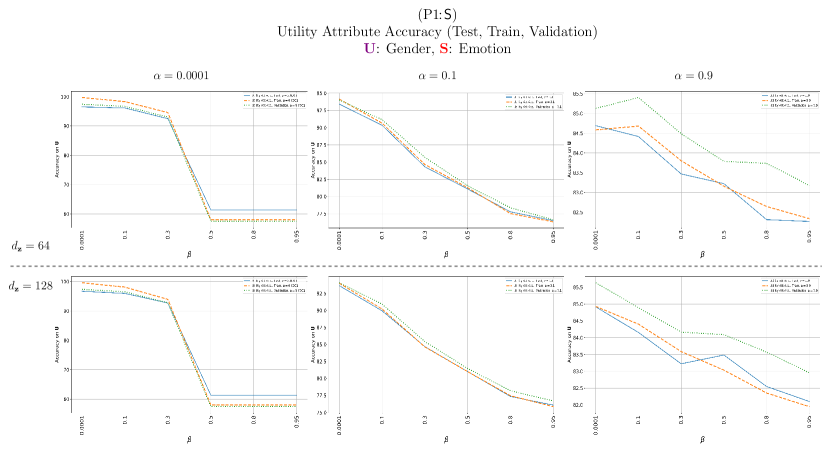
Figure 38: Recognition accuracy of the utility attribute $\mathbf{U}$ for supervised CLUB model ($\text{P1}\!\!:\!\mathsf{S}$) on ‘Test’, ‘Train’ and ‘Validation’ datasets of CelebA, considering $d_{\mathbf{z}}=64$ (First Row) and $d_{\mathbf{z}}=128$ (Second Row), setting $\mathbf{U}$: Gender, $\mathbf{S}$: Emotion (smiling), $Q_{\bm{\psi}}\!\left(\mathbf{Z}\right)=\mathcal{N}\!\left(\bm{0},\mathbf{I}_{d_{\mathbf{z}}}\right)$, for different information complexity weights $\beta$ and information leakage weights $\alpha$.

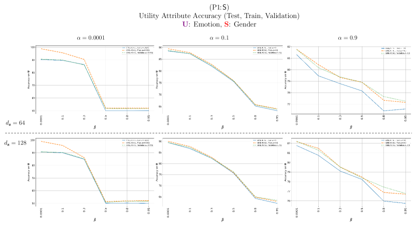
Figure 39: Recognition accuracy of the utility attribute $\mathbf{U}$ for supervised CLUB model ($\text{P1}\!\!:\!\mathsf{S}$) on ‘Test’, ‘Train’ and ‘Validation’ datasets of CelebA, considering $d_{\mathbf{z}}=64$ (First Row) and $d_{\mathbf{z}}=128$ (Second Row), setting $\mathbf{U}$: Emotion (smiling), $\mathbf{S}$: Gender, $Q_{\bm{\psi}}\!\left(\mathbf{Z}\right)=\mathcal{N}\!\left(\bm{0},\mathbf{I}_{d_{\mathbf{z}}}\right)$, for different information complexity weights $\beta$ and information leakage weights $\alpha$.

4.3 Training Algorithms

1:Input: Training Dataset: $\{\left(\mathbf{u}_{n},\mathbf{s}_{n},\mathbf{x}_{n}\right)\}_{n=1}^{N}$; Hyper-Parameters: $\gamma,\lambda$

2:$\bm{\phi},\bm{\theta},\bm{\psi},\bm{\xi},\bm{\eta},\bm{\omega},\bm{\tau}\;\leftarrow$ Initialize Network Parameters

3:repeat(1) Train the Encoder, Utility Decoder, Uncertainty Decoder $\left(\bm{\phi},\bm{\theta},\bm{\xi}\right)$

4:      Sample a mini-batch $\{\mathbf{u}_{m},\mathbf{s}_{m},\mathbf{x}_{m}\}_{m=1}^{M}\sim P_{\mathsf{D}}(\mathbf{X})P_{\mathbf{U},\mathbf{S}\mid\mathbf{X}}$

5:      Compute $\mathbf{z}_{m}\sim f_{\bm{\phi}}(\mathbf{x}_{m}),\forall m\in[M]$

6:      Back-propagate loss: $\mathcal{L}\!\left(\bm{\phi},\!\bm{\theta},\!\bm{\xi}\right)\!=\!\!-\frac{1}{M}\!\sum_{m=1}^{M}\!\!\big{(}\mathrm{D}_{\mathrm{KL}}\!\left(P_{\bm{\phi}}(\mathbf{z}_{m}\!\mid\!\mathbf{x}_{m})\|Q_{\bm{\psi}}(\mathbf{z}_{m})\right)-\gamma\log P_{\bm{\theta}}(\mathbf{u}_{m}\!\mid\!\mathbf{z}_{m})\!+\!\lambda\log P_{\bm{\xi}}(\mathbf{s}_{m}\!\mid\!\mathbf{z}_{m})\big{)}$ (2) Train the Latent Space Discriminator $\bm{\eta}$

7:      Sample $\{\mathbf{x}_{m}\}_{m=1}^{M}\sim P_{\mathsf{D}}(\mathbf{X})$

8:      Sample $\{\mathbf{n}_{m}\}_{m=1}^{M}\sim\mathcal{N}(\bm{0},\mathbf{I})$

9:      Compute $\mathbf{z}_{m}\sim f_{\bm{\phi}}(\mathbf{x}_{m}),\forall m\in[M]$

10:      Compute $\mathbf{\widetilde{z}}_{m}\sim g_{\bm{\psi}}(\mathbf{n}_{m}),\forall m\in[M]$

11:      Back-propagate loss: $\;\;\;\;\mathcal{L}\!\left(\bm{\eta}\right)\!=\!-\frac{1}{M}\sum_{m=1}^{M}\!\left(\log D_{\bm{\eta}}(\mathbf{z}_{m})\right)-\frac{1}{M}\sum_{m=1}^{M}\!\left(\log\left(1-D_{\bm{\eta}}(\,\mathbf{\widetilde{z}}_{m}\,)\right)\right)$ (3) Train the Encoder and Prior Distribution Generator $\left(\bm{\phi},\bm{\psi}\right)$ Adversarially

12:      Sample $\{\mathbf{x}_{m}\}_{m=1}^{M}\sim P_{\mathsf{D}}(\mathbf{X})$

13:      Sample $\{\mathbf{n}_{m}\}_{m=1}^{M}\sim\mathcal{N}(\bm{0},\mathbf{I})$

14:      Compute $\mathbf{z}_{m}\sim f_{\bm{\phi}}(\mathbf{x}_{m}),\forall m\in[M]$

15:      Compute $\mathbf{\widetilde{z}}_{m}\sim g_{\bm{\psi}}(\mathbf{n}_{m}),\forall m\in[M]$

16:      Back-propagate loss: $\;\;\;\;\mathcal{L}\!\left(\bm{\phi},\bm{\psi}\right)\!=\!\frac{1}{M}\sum_{m=1}^{M}\!\left(\log D_{\bm{\eta}}(\mathbf{z}_{m})\right)+\frac{1}{M}\sum_{m=1}^{M}\!\left(\log\left(1-D_{\bm{\eta}}(\,\mathbf{\widetilde{z}}_{m}\,)\right)\right)$ (4) Train the Utility Attribute Class Discriminator $\bm{\omega}$

17:      Sample $\{\mathbf{u}_{m}\}_{m=1}^{M}\sim P_{\mathbf{U}}$

18:      Sample $\{\mathbf{n}_{m}\}_{m=1}^{M}\sim\mathcal{N}\!\left(\bm{0},\mathbf{I}\right)$

19:      Compute $\mathbf{\widetilde{u}}_{m}\sim g_{\bm{\theta}}\left(g_{\bm{\psi}}(\mathbf{n}_{m})\right),\forall m\in[M]$

20:      Back-propagate loss: $\;\;\;\;\mathcal{L}\!\left(\bm{\omega}\right)\!=\!\gamma\left[-\frac{1}{M}\sum_{m=1}^{M}\!\left(\log D_{\bm{\omega}}(\mathbf{u}_{m})\right)-\frac{1}{M}\sum_{m=1}^{M}\!\left(\log\left(1-D_{\bm{\omega}}(\,\mathbf{\widetilde{u}}_{m}\,)\right)\right)\right]$ (5) Train the Sensitive Attribute Class Discriminator $\bm{\tau}$

21:      Sample $\{\mathbf{s}_{m}\}_{m=1}^{M}\sim P_{\mathbf{S}}$

22:      Sample $\{\mathbf{n}_{m}\}_{m=1}^{M}\sim\mathcal{N}\!\left(\bm{0},\mathbf{I}\right)$

23:      Compute $\mathbf{\widetilde{s}}_{m}\sim g_{\bm{\xi}}\left(g_{\bm{\psi}}(\mathbf{n}_{m})\right),\forall m\in[M]$

24:      Back-propagate loss: $\;\;\;\;\mathcal{L}\!\left(\bm{\tau}\right)\!=\!\lambda\left[\frac{1}{M}\sum_{m=1}^{M}\!\left(\log D_{\bm{\tau}}(\mathbf{s}_{m})\right)+\frac{1}{M}\sum_{m=1}^{M}\!\left(\log\left(1-D_{\bm{\tau}}(\,\mathbf{\widetilde{s}}_{m}\,)\right)\right)\right]$ (6) Train the Prior Distribution Generator, Utility Decoder, and Uncertainty Decoder $\left(\bm{\psi},\bm{\theta},\bm{\xi}\right)$ Adversarially

25:      Sample $\{\mathbf{n}_{m}\}_{m=1}^{M}\sim\mathcal{N}\!\left(\bm{0},\mathbf{I}\right)$

26:      Compute $\mathbf{\widetilde{u}}_{m}\sim g_{\bm{\theta}}\left(g_{\bm{\psi}}(\mathbf{n}_{m})\right),\forall m\in[M]$

27:      Compute $\mathbf{\widetilde{s}}_{m}\sim g_{\bm{\xi}}\left(g_{\bm{\psi}}(\mathbf{n}_{m})\right),\forall m\in[M]$

28:      Back-propagate loss: $\;\;\;\;\mathcal{L}\!\left(\bm{\psi},\bm{\theta},\bm{\xi}\right)\!=\!\gamma\,\frac{1}{M}\sum_{m=1}^{M}\!\left(\log\left(1-D_{\bm{\omega}}(\,\mathbf{\widetilde{u}}_{m}\,)\right)\right)-\lambda\,\frac{1}{M}\sum_{m=1}^{M}\!\left(\log\left(1-D_{\bm{\tau}}(\,\mathbf{\widetilde{s}}_{m}\,)\right)\right)$

29:until Convergence

30:return $\bm{\phi},\bm{\theta},\bm{\psi},\bm{\xi},\bm{\eta},\bm{\omega},\bm{\tau}$

Algorithm 3 Supervised Deep Variational CLUB training algorithm associated with ($\text{P3}\!\!:\!\mathsf{S}$)

1:Input: Training Dataset: $\{\left(\mathbf{s}_{n},\mathbf{x}_{n}\right)\}_{n=1}^{N}$; Hyper-Parameters: $\gamma,\lambda$

2:$\bm{\phi},\bm{\theta},\bm{\psi},\bm{\xi},\bm{\eta},\bm{\omega},\bm{\tau}\;\leftarrow$ Initialize Network Parameters

3:repeat(1) Train the Encoder, Utility Decoder, Uncertainty Decoder $\left(\bm{\phi},\bm{\theta},\bm{\xi}\right)$

4:      Sample a mini-batch $\{\mathbf{s}_{m},\mathbf{x}_{m}\}_{m=1}^{M}\sim P_{\mathsf{D}}(\mathbf{X})P_{\mathbf{S}\mid\mathbf{X}}$

5:      Compute $\mathbf{z}_{m}\sim f_{\bm{\phi}}(\mathbf{x}_{m}),\forall m\in[M]$

6:      Back-propagate loss: $\mathcal{L}\!\left(\bm{\phi},\!\bm{\theta},\!\bm{\xi}\right)\!=\!\!-\frac{1}{M}\!\sum_{m=1}^{M}\!\!\big{(}\mathrm{D}_{\mathrm{KL}}\!\left(P_{\bm{\phi}}(\mathbf{z}_{m}\!\mid\!\mathbf{x}_{m})\|Q_{\bm{\psi}}(\mathbf{z}_{m})\right)-\gamma\log P_{\bm{\theta}}(\mathbf{x}_{m}\!\mid\!\mathbf{z}_{m})\!+\!\lambda\log P_{\bm{\xi}}(\mathbf{s}_{m}\!\mid\!\mathbf{z}_{m})\big{)}$ (2) Train the Latent Space Discriminator $\bm{\eta}$

7:      Sample $\{\mathbf{x}_{m}\}_{m=1}^{M}\sim P_{\mathsf{D}}(\mathbf{X})$

8:      Sample $\{\mathbf{n}_{m}\}_{m=1}^{M}\sim\mathcal{N}(\bm{0},\mathbf{I})$

9:      Compute $\mathbf{z}_{m}\sim f_{\bm{\phi}}(\mathbf{x}_{m}),\forall m\in[M]$

10:      Compute $\mathbf{\widetilde{z}}_{m}\sim g_{\bm{\psi}}(\mathbf{n}_{m}),\forall m\in[M]$

11:      Back-propagate loss: $\;\;\;\;\mathcal{L}\!\left(\bm{\eta}\right)\!=\!-\frac{1}{M}\sum_{m=1}^{M}\!\left(\log D_{\bm{\eta}}(\mathbf{z}_{m})\right)-\frac{1}{M}\sum_{m=1}^{M}\!\left(\log\left(1-D_{\bm{\eta}}(\,\mathbf{\widetilde{z}}_{m}\,)\right)\right)$ (3) Train the Encoder and Prior Distribution Generator $\left(\bm{\phi},\bm{\psi}\right)$ Adversarially

12:      Sample $\{\mathbf{x}_{m}\}_{m=1}^{M}\sim P_{\mathsf{D}}(\mathbf{X})$

13:      Sample $\{\mathbf{n}_{m}\}_{m=1}^{M}\sim\mathcal{N}(\bm{0},\mathbf{I})$

14:      Compute $\mathbf{z}_{m}\sim f_{\bm{\phi}}(\mathbf{x}_{m}),\forall m\in[M]$

15:      Compute $\mathbf{\widetilde{z}}_{m}\sim g_{\bm{\psi}}(\mathbf{n}_{m}),\forall m\in[M]$

16:      Back-propagate loss: $\;\;\;\;\mathcal{L}\!\left(\bm{\phi},\bm{\psi}\right)\!=\!\frac{1}{M}\sum_{m=1}^{M}\!\left(\log D_{\bm{\eta}}(\mathbf{z}_{m})\right)+\frac{1}{M}\sum_{m=1}^{M}\!\left(\log\left(1-D_{\bm{\eta}}(\,\mathbf{\widetilde{z}}_{m}\,)\right)\right)$ (4) Train the Visible Space Discriminator $\bm{\omega}$

17:      Sample $\{\mathbf{x}_{m}\}_{m=1}^{M}\sim P_{\mathsf{D}}(\mathbf{X})$

18:      Sample $\{\mathbf{n}_{m}\}_{m=1}^{M}\sim\mathcal{N}\!\left(\bm{0},\mathbf{I}\right)$

19:      Compute $\mathbf{\widetilde{x}}_{m}\sim g_{\bm{\theta}}\left(g_{\bm{\psi}}(\mathbf{n}_{m})\right),\forall m\in[M]$

20:      Back-propagate loss: $\;\;\;\;\mathcal{L}\!\left(\bm{\omega}\right)\!=\!\gamma\left[-\frac{1}{M}\sum_{m=1}^{M}\!\left(\log D_{\bm{\omega}}(\mathbf{x}_{m})\right)-\frac{1}{M}\sum_{m=1}^{M}\!\left(\log\left(1-D_{\bm{\omega}}(\,\mathbf{\widetilde{x}}_{m}\,)\right)\right)\right]$ (5) Train the Sensitive Attribute Class Discriminator $\bm{\tau}$

21:      Sample $\{\mathbf{s}_{m}\}_{m=1}^{M}\sim P_{\mathbf{S}}$

22:      Sample $\{\mathbf{n}_{m}\}_{m=1}^{M}\sim\mathcal{N}\!\left(\bm{0},\mathbf{I}\right)$

23:      Compute $\mathbf{\widetilde{s}}_{m}\sim g_{\bm{\xi}}\left(g_{\bm{\psi}}(\mathbf{n}_{m})\right),\forall m\in[M]$

24:      Back-propagate loss: $\;\;\;\;\mathcal{L}\!\left(\bm{\tau}\right)\!=\!\lambda\left[\frac{1}{M}\sum_{m=1}^{M}\!\left(\log D_{\bm{\tau}}(\mathbf{s}_{m})\right)+\frac{1}{M}\sum_{m=1}^{M}\!\left(\log\left(1-D_{\bm{\tau}}(\,\mathbf{\widetilde{s}}_{m}\,)\right)\right)\right]$ (6) Train the Prior Distribution Generator, Utility Decoder, and Uncertainty Decoder $\left(\bm{\psi},\bm{\theta},\bm{\xi}\right)$ Adversarially

25:      Sample $\{\mathbf{n}_{m}\}_{m=1}^{M}\sim\mathcal{N}\!\left(\bm{0},\mathbf{I}\right)$

26:      Compute $\mathbf{\widetilde{x}}_{m}\sim g_{\bm{\theta}}\left(g_{\bm{\psi}}(\mathbf{n}_{m})\right),\forall m\in[M]$

27:      Compute $\mathbf{\widetilde{s}}_{m}\sim g_{\bm{\xi}}\left(g_{\bm{\psi}}(\mathbf{n}_{m})\right),\forall m\in[M]$

28:      Back-propagate loss: $\;\;\;\;\mathcal{L}\!\left(\bm{\psi},\bm{\theta},\bm{\xi}\right)\!=\!\gamma\,\frac{1}{M}\sum_{m=1}^{M}\!\left(\log\left(1-D_{\bm{\omega}}(\,\mathbf{\widetilde{x}}_{m}\,)\right)\right)-\lambda\,\frac{1}{M}\sum_{m=1}^{M}\!\left(\log\left(1-D_{\bm{\tau}}(\,\mathbf{\widetilde{s}}_{m}\,)\right)\right)$

29:until Convergence

30:return $\bm{\phi},\bm{\theta},\bm{\psi},\bm{\xi},\bm{\eta},\bm{\omega},\bm{\tau}$

Algorithm 4 Unsupervised Deep Variational CLUB training algorithm associated with ($\text{P3}\!\!:\!\mathsf{U}$)

References

• [1] F. P. Calmon and N. Fawaz, “Privacy against statistical inference,” in 50th Annual Allerton Conference on Communication, Control, and Computing.   IEEE, 2012, pp. 1401–1408.
• [2] A. Makhdoumi, S. Salamatian, N. Fawaz, and M. Médard, “From the information bottleneck to the privacy funnel,” in IEEE Information Theory Workshop (ITW).   IEEE, 2014, pp. 501–505.
• [3] N. Tishby, F. C. Pereira, and W. Bialek, “The information bottleneck method,” in IEEE Allerton, 2000.
• [4] C. T. Li and A. El Gamal, “Extended Gray–Wyner system with complementary causal side information,” IEEE Transactions on Information Theory, vol. 64, no. 8, pp. 5862–5878, 2017.
• [5] C. Louizos, K. Swersky, Y. Li, M. Welling, and R. Zemel, “The variational fair autoencoder,” in International Conference on Learning Representation (ICLR), 2016.
• [6] C. Dwork, M. Hardt, T. Pitassi, O. Reingold, and R. Zemel, “Fairness through awareness,” in 3rd Innovations in Theoretical Computer Science Conference, 2012, pp. 214–226.
• [7] F. Kamiran and T. Calders, “Data preprocessing techniques for classification without discrimination,” Knowledge and Information Systems, vol. 33, no. 1, pp. 1–33, 2012.
• [8] R. Zemel, Y. Wu, K. Swersky, T. Pitassi, and C. Dwork, “Learning fair representations,” in International Conference on Machine Learning (ICML), 2013, pp. 325–333.
• [9] M. Hardt, E. Price, and N. Srebro, “Equality of opportunity in supervised learning,” in Advances in Neural Information Processing Systems, 2016, pp. 3315–3323.
• [10] F. P. Calmon, D. Wei, B. Vinzamuri, K. N. Ramamurthy, and K. R. Varshney, “Optimized pre-processing for discrimination prevention,” in Advances in Neural Information Processing Systems, 2017, pp. 3992–4001.
• [11] M. B. Zafar, I. Valera, M. G. Rogriguez, and K. P. Gummadi, “Fairness constraints: Mechanisms for fair classification,” in Artificial Intelligence and Statistics.   PMLR, 2017, pp. 962–970.
• [12] G. Louppe, M. Kagan, and K. Cranmer, “Learning to pivot with adversarial networks,” in Advances in Neural Information Processing Systems, 2017, pp. 981–990.
• [13] C. Wadsworth, F. Vera, and C. Piech, “Achieving fairness through adversarial learning: an application to recidivism prediction,” arXiv preprint arXiv:1807.00199, 2018.
• [14] B. H. Zhang, B. Lemoine, and M. Mitchell, “Mitigating unwanted biases with adversarial learning,” in AAAI/ACM Conference on AI, Ethics, and Society, 2018, pp. 335–340.
• [15] D. P. Kingma and M. Welling, “Auto-encoding variational bayes,” in International Conference on Learning Representations (ICLR), 2014.
• [16] I. Higgins, L. Matthey, A. Pal, C. Burgess, X. Glorot, M. Botvinick, S. Mohamed, and A. Lerchner, “beta-vae: Learning basic visual concepts with a constrained variational framework,” in International Conference on Learning Representations (ICLR), 2017.
• [17] “Infovae: Information maximizing variational autoencoders,” arXiv preprint arXiv:1706.02262, 2017.
• [18] I. Goodfellow, J. Pouget-Abadie, M. Mirza, B. Xu, D. Warde-Farley, S. Ozair, A. Courville, and Y. Bengio, “Generative adversarial nets,” in Advances in neural information processing systems, 2014, pp. 2672–2680.
• [19] M. Arjovsky, S. Chintala, and L. Bottou, “Wasserstein gan,” arXiv preprint arXiv:1701.07875, 2017.
• [20] I. Tolstikhin, O. Bousquet, S. Gelly, and B. Schölkopf, “Wasserstein auto-encoders,” in International Conference on Learning Representations (ICLR), 2018.
• [21] A. Makhzani, J. Shlens, N. Jaitly, I. Goodfellow, and B. Frey, “Adversarial autoencoders,” arXiv preprint arXiv:1511.05644, 2015.
• [22] A. B. L. Larsen, S. K. Sønderby, H. Larochelle, and O. Winther, “Autoencoding beyond pixels using a learned similarity metric,” in International Conference on Machine Learning, 2016, pp. 1558–1566.
• [23] S. Voloshynovskiy, M. Kondah, S. Rezaeifar, O. Taran, T. Hotolyak, and D. J. Rezende, “Information bottleneck through variational glasses,” in NeurIPS Workshop on Bayesian Deep Learning, Vancouver, Canada, December 2019.
• [24] L. Sweeney, “Simple demographics often identify people uniquely,” Health (San Francisco), vol. 671, pp. 1–34, 2000.
• [25] ——, “k-anonymity: A model for protecting privacy,” International Journal of Uncertainty, Fuzziness and Knowledge-Based Systems, vol. 10, no. 05, pp. 557–570, 2002.
• [26] A. Machanavajjhala, J. Gehrke, D. Kifer, and M. Venkitasubramaniam, “l-diversity: Privacy beyond k-anonymity,” in Data Engineering, 2006. ICDE’06. Proceedings of the 22nd International Conference on.   IEEE, 2006, pp. 24–24.
• [27] N. Li, T. Li, and S. Venkatasubramanian, “t-closeness: Privacy beyond k-anonymity and l-diversity,” in IEEE 23rd International Conference on Data Engineering (ICDE).   IEEE, 2007, pp. 106–115.
• [28] C. Dwork, F. McSherry, K. Nissim, and A. Smith, “Calibrating noise to sensitivity in private data analysis,” in Theory of Cryptography Conference.   Springer, 2006, pp. 265–284.
• [29] D. Kifer and A. Machanavajjhala, “A rigorous and customizable framework for privacy,” in 31st ACM SIGMOD-SIGACT-SIGAI symposium on Principles of Database Systems.   ACM, 2012, pp. 77–88.
• [30] I. S. Reed, “Information theory and privacy in data banks,” in National Computer Conference and Exposition.   ACM, 1973, pp. 581–587.
• [31] H. Yamamoto, “A source coding problem for sources with additional outputs to keep secret from the receiver or wiretappers (corresp.),” IEEE Transactions on Information Theory, vol. 29, no. 6, pp. 918–923, 1983.
• [32] A. Evfimievski, J. Gehrke, and R. Srikant, “Limiting privacy breaches in privacy preserving data mining,” in 22th ACM SIGMOD-SIGACT-SIGART symposium on Principles of database systems.   ACM, 2003, pp. 211–222.
• [33] D. Rebollo-Monedero, J. Forne, and J. Domingo-Ferrer, “From t-closeness-like privacy to postrandomization via information theory,” IEEE Transactions on Knowledge and Data Engineering, vol. 22, no. 11, pp. 1623–1636, 2009.
• [34] L. Sankar, S. R. Rajagopalan, and H. V. Poor, “Utility-privacy tradeoffs in databases: An information-theoretic approach,” IEEE Transactions on Information Forensics and Security (TIFS), vol. 8, no. 6, pp. 838–852, 2013.
• [35] F. P. Calmon, M. Varia, M. Médard, M. M. Christiansen, K. R. Duffy, and S. Tessaro, “Bounds on inference,” in 51st Annual Allerton Conference on Communication, Control, and Computing.   IEEE, 2013, pp. 567–574.
• [36] A. Makhdoumi and N. Fawaz, “Privacy-utility tradeoff under statistical uncertainty,” in 51st Annual Allerton Conference on Communication, Control, and Computing.   IEEE, 2013, pp. 1627–1634.
• [37] S. Asoodeh, F. Alajaji, and T. Linder, “Notes on information-theoretic privacy,” in 52nd Annual Allerton Conference on Communication, Control, and Computing.   IEEE, 2014, pp. 1272–1278.
• [38] F. P. Calmon, A. Makhdoumi, and M. Médard, “Fundamental limits of perfect privacy,” in IEEE International Symposium on Information Theory (ISIT).   IEEE, 2015, pp. 1796–1800.
• [39] S. Salamatian, A. Zhang, F. P. Calmon, S. Bhamidipati, N. Fawaz, B. Kveton, P. Oliveira, and N. Taft, “Managing your private and public data: Bringing down inference attacks against your privacy,” IEEE Journal of Selected Topics in Signal Processing, vol. 9, no. 7, pp. 1240–1255, 2015.
• [40] Y. O. Basciftci, Y. Wang, and P. Ishwar, “On privacy-utility tradeoffs for constrained data release mechanisms,” in Information Theory and Applications Workshop (ITA).   IEEE, 2016, pp. 1–6.
• [41] S. Asoodeh, M. Diaz, F. Alajaji, and T. Linder, “Information extraction under privacy constraints,” Information, vol. 7, no. 1, p. 15, 2016.
• [42] K. Kalantari, L. Sankar, and O. Kosut, “On information-theoretic privacy with general distortion cost functions,” in IEEE International Symposium on Information Theory (ISIT).   IEEE, 2017, pp. 2865–2869.
• [43] B. Rassouli, F. Rosas, and D. Gündüz, “Latent feature disclosure under perfect sample privacy,” in IEEE International Workshop on Information Forensics and Security (WIFS).   IEEE, 2018, pp. 1–7.
• [44] S. Asoodeh, M. Diaz, F. Alajaji, and T. Linder, “Estimation efficiency under privacy constraints,” IEEE Transactions on Information Theory, vol. 65, no. 3, pp. 1512–1534, 2018.
• [45] B. Rassouli and D. Gündüz, “On perfect privacy,” in IEEE International Symposium on Information Theory (ISIT).   IEEE, 2018, pp. 2551–2555.
• [46] J. Liao, O. Kosut, L. Sankar, and F. P. Calmon, “Privacy under hard distortion constraints,” in IEEE Information Theory Workshop (ITW).   IEEE, 2018, pp. 1–5.
• [47] S. A. Osia, A. Taheri, A. S. Shamsabadi, K. Katevas, H. Haddadi, and H. R. Rabiee, “Deep private-feature extraction,” IEEE Transactions on Knowledge and Data Engineering, vol. 32, no. 1, pp. 54–66, 2018.
• [48] A. Tripathy, Y. Wang, and P. Ishwar, “Privacy-preserving adversarial networks,” in 57th Annual Allerton Conference on Communication, Control, and Computing.   IEEE, 2019, pp. 495–505.
• [49] H. Hsu, S. Asoodeh, F. P. Calmon, and N. Fawaz, “Information-theoretic privacy watchdogs,” in IEEE International Symposium on Information Theory (ISIT).   IEEE, 2019.
• [50] J. Liao, O. Kosut, L. Sankar, and F. P. Calmon, “Tunable measures for information leakage and applications to privacy-utility tradeoffs,” IEEE Transactions on Information Theory, vol. 65, no. 12, pp. 8043–8066, 2019.
• [51] S. Sreekumar and D. Gündüz, “Optimal privacy-utility trade-off under a rate constraint,” in IEEE International Symposium on Information Theory (ISIT).   IEEE, 2019, pp. 2159–2163.
• [52] T. Xiao and A. Khisti, “Maximal information leakage based privacy preserving data disclosure mechanisms,” in 16th Canadian Workshop on Information Theory (CWIT).   IEEE, 2019, pp. 1–6.
• [53] M. Diaz, H. Wang, F. P. Calmon, and L. Sankar, “On the robustness of information-theoretic privacy measures and mechanisms,” IEEE Transactions on Information Theory, vol. 66, no. 4, pp. 1949–1978, 2019.
• [54] B. Rassouli, F. E. Rosas, and D. Gündüz, “Data disclosure under perfect sample privacy,” IEEE Transactions on Information Forensics and Security, 2019.
• [55] B. Rassouli and D. Gündüz, “Optimal utility-privacy trade-off with total variation distance as a privacy measure,” IEEE Transactions on Information Forensics and Security, vol. 15, pp. 594–603, 2019.
• [56] ——, “On perfect privacy,” IEEE Journal on Selected Areas in Information Theory, vol. 2, no. 1, pp. 177–191, 2021.
• [57] C. E. Shannon, “Communication theory of secrecy systems,” Bell system technical journal, vol. 28, no. 4, pp. 656–715, 1949.
• [58] H. Edwards and A. Storkey, “Censoring representations with an adversary,” in International Conference on Learning Representation (ICLR), 2016.
• [59] J. Hamm, “Enhancing utility and privacy with noisy minimax filters,” in IEEE International Conference on Acoustics, Speech and Signal Processing (ICASSP).   IEEE, 2017, pp. 6389–6393.
• [60] C. Huang, P. Kairouz, X. Chen, L. Sankar, and R. Rajagopal, “Context-aware generative adversarial privacy,” Entropy, vol. 19, no. 12, p. 656, 2017.
• [61] ——, “Generative adversarial privacy,” arXiv preprint arXiv:1807.05306, 2018.
• [62] M. Bertran, N. Martinez, A. Papadaki, Q. Qiu, M. Rodrigues, G. Reeves, and G. Sapiro, “Adversarially learned representations for information obfuscation and inference,” in International Conference on Machine Learning, 2019, pp. 614–623.
• [63] B. Razeghi, F. P. Calmon, D. Gündüz, and S. Voloshynovskiy, “On perfect obfuscation: Local information geometry analysis,” in IEEE International Workshop on Information Forensics and Security (WIFS), 2020, pp. 1–6.
• [64] A. A. Atashin, B. Razeghi, D. Gündüz, and S. Voloshynovskiy, “Variational leakage: The role of information complexity in privacy leakage,” in 3rd ACM Workshop on Wireless Security and Machine Learning, 2021, pp. 91–96.
• [65] N. Cesa-Bianchi and G. Lugosi, Prediction, learning, and games.   Cambridge university press, 2006.
• [66] T. Andre, M. Antonini, M. Barlaud, and R. M. Gray, “Entropy-based distortion measure for image coding,” in International Conference on Image Processing.   IEEE, 2006, pp. 1157–1160.
• [67] P. Harremoës and N. Tishby, “The information bottleneck revisited or how to choose a good distortion measure,” in IEEE International Symposium on Information Theory.   IEEE, 2007, pp. 566–570.
• [68] T. A. Courtade and R. D. Wesel, “Multiterminal source coding with an entropy-based distortion measure,” in IEEE International Symposium on Information Theory (ISIT).   IEEE, 2011, pp. 2040–2044.
• [69] T. M. Cover, Elements of information theory.   John Wiley & Sons, 1999.
• [70] Y. Polyanskiy and Y. Wu, “Lecture notes on information theory,” Lecture Notes for ECE563 (UIUC) and, vol. 6, 2014.
• [71] S. Arimoto, “Information measures and capacity of order $\alpha$ for discrete memoryless channels,” Topics in information theory, 1977.
• [72] I. Csiszár, “Information-type measures of difference of probability distributions and indirect observation,” studia scientiarum Mathematicarum Hungarica, vol. 2, pp. 229–318, 1967.
• [73] J. Duchi, “Lecture notes for statistics 311/electrical engineering 377,” 2016.
• [74] J. Rissanen, “Stochastic complexity and modeling,” The annals of statistics, pp. 1080–1100, 1986.
• [75] ——, “Stochastic complexity,” Journal of the Royal Statistical Society: Series B (Methodological), vol. 49, no. 3, pp. 223–239, 1987.
• [76] J. J. Rissanen, “Fisher information and stochastic complexity,” IEEE Transactions on Information Theory, vol. 42, no. 1, pp. 40–47, 1996.
• [77] P. D. Grünwald, I. J. Myung, and M. A. Pitt, Advances in minimum description length: Theory and applications, 2005.
• [78] P. Grunwald, “A tutorial introduction to the minimum description length principle,” arXiv preprint math/0406077, 2004.
• [79] M. Vera, P. Piantanida, and L. R. Vega, “The role of information complexity and randomization in representation learning,” arXiv preprint arXiv:1802.05355, 2018.
• [80] ——, “The role of the information bottleneck in representation learning,” in IEEE International Symposium on Information Theory (ISIT).   IEEE, 2018, pp. 1580–1584.
• [81] I. Fischer, “The conditional entropy bottleneck,” arXiv preprint arXiv:2002.05379, 2020.
• [82] B. Rodríguez-Gálvez, R. Thobaben, and M. Skoglund, “A variational approach to privacy and fairness,” arXiv preprint arXiv:2006.06332, 2020.
• [83] D. P. Kingma, T. Salimans, R. Jozefowicz, X. Chen, I. Sutskever, and M. Welling, “Improved variational inference with inverse autoregressive flow,” in Advances in Neural Information Processing Systems, 2016, pp. 4743–4751.
• [84] D. J. Rezende and S. Mohamed, “Variational inference with normalizing flows,” in 32nd International Conference on Machine Learning, 2015, pp. 1530–1538.
• [85] M. Rosca, B. Lakshminarayanan, and S. Mohamed, “Distribution matching in variational inference,” arXiv preprint arXiv:1802.06847, 2018.
• [86] J. Tomczak and M. Welling, “VAE with a VampPrior,” in International Conference on Artificial Intelligence and Statistics, 2018, pp. 1214–1223.
• [87] M. Bauer and A. Mnih, “Resampled priors for variational autoencoders,” in 22nd International Conference on Artificial Intelligence and Statistics, 2019, pp. 66–75.
• [88] N. Dilokthanakul, P. A. Mediano, M. Garnelo, M. C. Lee, H. Salimbeni, K. Arulkumaran, and M. Shanahan, “Deep unsupervised clustering with gaussian mixture variational autoencoders,” arXiv preprint arXiv:1611.02648, 2016.
• [89] E. Nalisnick, L. Hertel, and P. Smyth, “Approximate inference for deep latent gaussian mixtures,” in NIPS Workshop on Bayesian Deep Learning, vol. 2, 2016.
• [90] L. Mescheder, S. Nowozin, and A. Geiger, “Adversarial variational bayes: unifying variational autoencoders and generative adversarial networks,” in International Conference on Machine Learning (ICML), 2017, pp. 2391–2400.
• [91] V. Dumoulin, I. Belghazi, B. Poole, O. Mastropietro, A. Lamb, M. Arjovsky, and A. Courville, “Adversarially learned inference,” in International Conference on Learning Representations (ICLR), 2017.
• [92] J. Donahue, P. Krähenbühl, and T. Darrell, “Adversarial feature learning,” in International Conference on Learning Representations (ICLR), 2017.
• [93] F. Huszár, “Variational inference using implicit distributions,” arXiv preprint arXiv:1702.08235, 2017.
• [94] X. Nguyen, M. J. Wainwright, and M. I. Jordan, “Estimating divergence functionals and the likelihood ratio by convex risk minimization,” IEEE Transactions on Information Theory, vol. 56, no. 11, pp. 5847–5861, 2010.
• [95] M. Sugiyama, T. Suzuki, and T. Kanamori, “Density-ratio matching under the Bregman divergence: A unified framework of density-ratio estimation,” Annals of the Institute of Statistical Mathematics, vol. 64, no. 5, pp. 1009–1044, 2012.
• [96] R. W. Yeung, “A new outlook on shannon’s information measures,” IEEE Transactions on Information Theory, vol. 37, no. 3, pp. 466–474, 1991.
• [97] A. Wyner and J. Ziv, “A theorem on the entropy of certain binary sequences and applications–i,” IEEE Transactions on Information Theory, vol. 19, no. 6, pp. 769–772, 1973.
• [98] A. Wyner, “A theorem on the entropy of certain binary sequences and applications–ii,” IEEE Transactions on Information Theory, vol. 19, no. 6, pp. 772–777, 1973.
• [99] H. Witsenhausen and A. Wyner, “A conditional entropy bound for a pair of discrete random variables,” IEEE Transactions on Information Theory, vol. 21, no. 5, pp. 493–501, 1975.
• [100] R. Ahlswede and J. Körner, “On the connection between the entropies of input and output distributions of discrete memoryless channels,” in 5th Conference on Probability Theory, 1977.
• [101] N. Tishby and N. Zaslavsky, “Deep learning and the information bottleneck principle,” in IEEE Information Theory Workshop (ITW).   IEEE, 2015, pp. 1–5.
• [102] A. A. Alemi, I. Fischer, J. V. Dillon, and K. Murphy, “Deep variational information bottleneck,” arXiv preprint arXiv:1612.00410, 2016.
• [103] D. Strouse and D. J. Schwab, “The deterministic information bottleneck,” Neural computation, vol. 29, no. 6, pp. 1611–1630, 2017.
• [104] M. Vera, L. R. Vega, and P. Piantanida, “Collaborative information bottleneck,” IEEE Transactions on Information Theory, vol. 65, no. 2, pp. 787–815, 2018.
• [105] A. Kolchinsky, B. D. Tracey, and S. Van Kuyk, “Caveats for information bottleneck in deterministic scenarios,” in International Conference on Learning Representations (ICLR), 2019.
• [106] S. Bang, P. Xie, H. Lee, W. Wu, and E. Xing, “Explaining a black-box using deep variational information bottleneck approach,” arXiv preprint arXiv:1902.06918, 2019.
• [107] R. A. Amjad and B. C. Geiger, “Learning representations for neural network-based classification using the information bottleneck principle,” IEEE Transactions on Pattern Analysis and Machine Intelligence, 2019.
• [108] J. Hu, R. Ji, S. Zhang, X. Sun, Q. Ye, C.-W. Lin, and Q. Tian, “Information competing process for learning diversified representations,” in Advances in Neural Information Processing Systems, 2019, pp. 2175–2186.
• [109] T. Wu, I. Fischer, I. L. Chuang, and M. Tegmark, “Learnability for the information bottleneck,” International Conference on Learning Representations (ICLR), 2019.
• [110] M. Federici, A. Dutta, P. Forré, N. Kushman, and Z. Akata, “Learning robust representations via multi-view information bottleneck,” International Conference on Learning Representations (ICLR), 2020.
• [111] N. Ding and P. Sadeghi, “A submodularity-based clustering algorithm for the information bottleneck and privacy funnel,” in IEEE Information Theory Workshop (ITW).   IEEE, 2019, pp. 1–5.
• [112] H. Hafez-Kolahi and S. Kasaei, “Information bottleneck and its applications in deep learning,” Algorithms, vol. 3, no. 4, p. 5, 2019.
• [113] H. Hafez-Kolahi, S. Kasaei, and M. Soleymani-Baghshah, “Sample complexity of classification with compressed input,” Neurocomputing, 2020.
• [114] A. Kirsch, C. Lyle, and Y. Gal, “Unpacking information bottlenecks: Unifying information-theoretic objectives in deep learning,” arXiv preprint arXiv:2003.12537, 2020.
• [115] S. Voloshynovskiy, M. Kondah, S. Rezaeifar, O. Taran, T. Holotyak, and D. J. Rezende, “Information bottleneck through variational glasses,” in 4th Workshop on Bayesian Deep Learning (NeurIPS 2019), 2019.
• [116] Z. Goldfeld and Y. Polyanskiy, “The information bottleneck problem and its applications in machine learning,” IEEE Journal on Selected Areas in Information Theory, 2020.
• [117] A. Zaidi, I. Estella-Aguerri et al., “On the information bottleneck problems: Models, connections, applications and information theoretic views,” Entropy, vol. 22, no. 2, p. 151, 2020.
• [118] S. Asoodeh and F. P. Calmon, “Bottleneck problems: An information and estimation-theoretic view,” Entropy, vol. 22, no. 11, p. 1325, 2020.
• [119] Y. Steinberg, “Coding and common reconstruction,” IEEE Transactions on Information Theory, vol. 55, no. 11, pp. 4995–5010, 2009.
• [120] M. Benammar and A. Zaidi, “Rate-distortion function for a heegard-berger problem with two sources and degraded reconstruction sets,” IEEE Transactions on Information Theory, vol. 62, no. 9, pp. 5080–5092, 2016.
• [121] M. Mirza and S. Osindero, “Conditional generative adversarial nets,” arXiv preprint arXiv:1411.1784, 2014.
• [122] T. Salimans, I. Goodfellow, W. Zaremba, V. Cheung, A. Radford, and X. Chen, “Improved techniques for training gans,” in Advances in neural information processing systems, 2016, pp. 2234–2242.
• [123] J. Ho and S. Ermon, “Generative adversarial imitation learning,” in Advances in neural information processing systems, 2016, pp. 4565–4573.
• [124] V. Dumoulin, I. Belghazi, B. Poole, O. Mastropietro, A. Lamb, M. Arjovsky, and A. Courville, “Adversarially learned inference,” arXiv preprint arXiv:1606.00704, 2016.
• [125] J. Zhao, M. Mathieu, and Y. LeCun, “Energy-based generative adversarial network,” arXiv preprint arXiv:1609.03126, 2016.
• [126] S. Nowozin, B. Cseke, and R. Tomioka, “f-gan: Training generative neural samplers using variational divergence minimization,” in Advances in neural information processing systems, 2016, pp. 271–279.
• [127] P. Isola, J.-Y. Zhu, T. Zhou, and A. A. Efros, “Image-to-image translation with conditional adversarial networks,” in IEEE Conference on Computer Vision and Pattern Recognition, 2017, pp. 1125–1134.
• [128] J.-Y. Zhu, T. Park, P. Isola, and A. A. Efros, “Unpaired image-to-image translation using cycle-consistent adversarial networks,” in IEEE International Conference on Computer Vision, 2017, pp. 2223–2232.
• [129] X. Mao, Q. Li, H. Xie, R. Y. Lau, Z. Wang, and S. Paul Smolley, “Least squares generative adversarial networks,” in IEEE International Conference on Computer Vision, 2017, pp. 2794–2802.
• [130] H. Zhang, I. Goodfellow, D. Metaxas, and A. Odena, “Self-attention generative adversarial networks,” in International Conference on Machine Learning.   PMLR, 2019, pp. 7354–7363.
• [131] Y. Wu, “Lecture notes for ECE598YW: Information-theoretic methods for high-dimensional statistics,” 2017.
• [132] C. Villani, Optimal transport: old and new.   Springer Science & Business Media, 2008, vol. 338.
• [133] G. Peyré, M. Cuturi et al., “Computational optimal transport: With applications to data science,” Foundations and Trends® in Machine Learning, vol. 11, no. 5-6, pp. 355–607, 2019.
• [134] O. Bousquet, S. Gelly, I. Tolstikhin, C.-J. Simon-Gabriel, and B. Schoelkopf, “From optimal transport to generative modeling: the vegan cookbook,” arXiv preprint arXiv:1705.07642, 2017.
• [135] C. E. Shannon, “A mathematical theory of communication,” The Bell system technical journal, vol. 27, no. 3, pp. 379–423, 1948.
• [136] V. K. Goyal, “Theoretical foundations of transform coding,” IEEE Signal Processing Magazine, vol. 18, no. 5, pp. 9–21, 2001.
• [137] N. Sonehara, “Image data compression using a neural network model,” in International Joint Conference on Neural Networks, 1989, pp. II–35.
• [138] S. P. Luttrell, “Image compression using a multilayer neural network.” Pattern Recognition Letters, vol. 10, no. 1, pp. 1–7, 1989.
• [139] D. Anthony, E. Hines, J. Barham, and D. Taylor, “A comparison of image compression by neural networks and principal component analysis,” in IJCNN International Joint Conference on Neural Networks.   IEEE, 1990, pp. 339–344.
• [140] G. Sicuranza, G. Romponi, and S. Marsi, “Artificial neural network for image compression,” Electronics Letters, vol. 26, no. 7, pp. 477–479, 1990.
• [141] R. Setiono and G. Lu, “Image compression using a feedforward neural network,” in IEEE International Conference on Neural Networks (ICNN), vol. 7.   IEEE, 1994, pp. 4761–4765.
• [142] R. D. Dony and S. Haykin, “Neural network approaches to image compression,” Proceedings of the IEEE, vol. 83, no. 2, pp. 288–303, 1995.
• [143] A. Namphol, S. H. Chin, and M. Arozullah, “Image compression with a hierarchical neural network,” IEEE Transactions on Aerospace and Electronic Systems, vol. 32, no. 1, pp. 326–338, 1996.
• [144] J. Jiang, “Image compression with neural networks–a survey,” Signal processing: image Communication, vol. 14, no. 9, pp. 737–760, 1999.
• [145] G. Toderici, S. M. O’Malley, S. J. Hwang, D. Vincent, D. Minnen, S. Baluja, M. Covell, and R. Sukthankar, “Variable rate image compression with recurrent neural networks,” in International Conference on Learning Representations (ICLR), 2016.
• [146] K. Gregor, F. Besse, D. Jimenez Rezende, I. Danihelka, and D. Wierstra, “Towards conceptual compression,” Advances In Neural Information Processing Systems, vol. 29, 2016.
• [147] J. Ballé, V. Laparra, and E. P. Simoncelli, “End-to-end optimized image compression,” in International Conference on Learning Representations (ICLR), 2017.
• [148] J. Ballé, D. Minnen, S. Singh, S. J. Hwang, and N. Johnston, “Variational image compression with a scale hyperprior,” in International Conference on Learning Representations (ICLR), 2017.
• [149] L. Theis, W. Shi, A. Cunningham, and F. Huszár, “Lossy image compression with compressive autoencoders,” in International Conference on Learning Representations (ICLR), 2017.
• [150] G. Toderici, D. Vincent, N. Johnston, S. Jin Hwang, D. Minnen, J. Shor, and M. Covell, “Full resolution image compression with recurrent neural networks,” in IEEE conference on Computer Vision and Pattern Recognition, 2017, pp. 5306–5314.
• [151] E. Agustsson, F. Mentzer, M. Tschannen, L. Cavigelli, R. Timofte, L. Benini, and L. V. Gool, “Soft-to-hard vector quantization for end-to-end learning compressible representations,” Advances in neural information processing systems, vol. 30, 2017.
• [152] O. Rippel and L. Bourdev, “Real-time adaptive image compression,” in International Conference on Machine Learning.   PMLR, 2017, pp. 2922–2930.
• [153] S. Santurkar, D. Budden, and N. Shavit, “Generative compression,” in Picture Coding Symposium (PCS).   IEEE, 2018, pp. 258–262.
• [154] F. Mentzer, E. Agustsson, M. Tschannen, R. Timofte, and L. Van Gool, “Conditional probability models for deep image compression,” in IEEE Conference on Computer Vision and Pattern Recognition, 2018, pp. 4394–4402.
• [155] M. Tschannen, E. Agustsson, and M. Lucic, “Deep generative models for distribution-preserving lossy compression,” Advances in Neural Information Processing Systems, vol. 31, 2018.
• [156] D. Minnen, J. Ballé, and G. D. Toderici, “Joint autoregressive and hierarchical priors for learned image compression,” Advances in neural information processing systems, vol. 31, 2018.
• [157] J. Ballé, D. Minnen, S. Singh, S. J. Hwang, and N. Johnston, “Variational image compression with a scale hyperprior,” in International Conference on Learning Representations (ICLR), 2018.
• [158] D. Ulyanov, A. Vedaldi, and V. Lempitsky, “Deep image prior,” in Proceedings of the IEEE conference on computer vision and pattern recognition, 2018, pp. 9446–9454.
• [159] E. Agustsson, M. Tschannen, F. Mentzer, R. Timofte, and L. V. Gool, “Generative adversarial networks for extreme learned image compression,” in IEEE/CVF International Conference on Computer Vision, 2019, pp. 221–231.
• [160] J. Lee, S. Cho, and S.-K. Beack, “Context-adaptive entropy model for end-to-end optimized image compression,” in International Conference on Learning Representations (ICLR), 2019.
• [161] Y. Choi, M. El-Khamy, and J. Lee, “Variable rate deep image compression with a conditional autoencoder,” in IEEE/CVF International Conference on Computer Vision, 2019, pp. 3146–3154.
• [162] Y. Hu, W. Yang, Z. Ma, and J. Liu, “Learning end-to-end lossy image compression: A benchmark,” IEEE Transactions on Pattern Analysis and Machine Intelligence, 2021.
• [163] Y. Yang, S. Mandt, and L. Theis, “An introduction to neural data compression,” arXiv preprint arXiv:2202.06533, 2022.
• [164] M. Gregorová, M. Desaules, and A. Kalousis, “Learned transform compression with optimized entropy encoding,” in ICLR Neural Compression Workshop, 2021.
• [165] H. Larochelle and I. Murray, “The neural autoregressive distribution estimator,” in 14th International Conference on Artificial Intelligence and Statistics.   JMLR Workshop and Conference Proceedings, 2011, pp. 29–37.
• [166] K. Ullrich, E. Meeds, and M. Welling, “Soft weight-sharing for neural network compression,” in International Conference on Learning Representations (ICLR), 2017.
• [167] D. G. Lowe, “Object recognition from local scale-invariant features,” in 7th IEEE international conference on computer vision, vol. 2.   IEEE, 1999, pp. 1150–1157.
• [168] D. Madras, E. Creager, T. Pitassi, and R. Zemel, “Fairness through causal awareness: Learning causal latent-variable models for biased data,” in Conference on Fairness, Accountability, and Transparency, 2019, pp. 349–358.
• [169] U. Hébert-Johnson, M. P. Kim, O. Reingold, and G. N. Rothblum, “Calibration for the (computationally-identifiable) masses,” arXiv preprint arXiv:1711.08513, 2017.
• [170] D. Madras, E. Creager, T. Pitassi, and R. Zemel, “Learning adversarially fair and transferable representations,” in International Conference on Machine Learning (ICML), 2018, pp. 3384–3393.
• [171] D. Madras, T. Pitassi, and R. Zemel, “Predict responsibly: improving fairness and accuracy by learning to defer,” in Advances in Neural Information Processing Systems, 2018, pp. 6147–6157.
• [172] M. Kearns, S. Neel, A. Roth, and Z. S. Wu, “Preventing fairness gerrymandering: Auditing and learning for subgroup fairness,” in International Conference on Machine Learning, 2018, pp. 2564–2572.
• [173] M. P. Kim, A. Ghorbani, and J. Zou, “Multiaccuracy: Black-box post-processing for fairness in classification,” in AAAI/ACM Conference on AI, Ethics, and Society, 2019, pp. 247–254.
• [174] L. E. Celis, L. Huang, V. Keswani, and N. K. Vishnoi, “Classification with fairness constraints: A meta-algorithm with provable guarantees,” in Conference on Fairness, Accountability, and Transparency, 2019, pp. 319–328.
• [175] R. K. Bellamy, K. Dey, M. Hind, S. C. Hoffman, S. Houde, K. Kannan, P. Lohia, J. Martino, S. Mehta, A. Mojsilović et al., “Ai fairness 360: An extensible toolkit for detecting and mitigating algorithmic bias,” IBM Journal of Research and Development, vol. 63, no. 4/5, pp. 4–1, 2019.
• [176] J. Chen, N. Kallus, X. Mao, G. Svacha, and M. Udell, “Fairness under unawareness: Assessing disparity when protected class is unobserved,” in Conference on Fairness, Accountability, and Transparency, 2019, pp. 339–348.
• [177] A. Grover, K. Choi, R. Shu, and S. Ermon, “Fair generative modeling via weak supervision,” arXiv preprint arXiv:1910.12008, 2019.
• [178] N. Mehrabi, F. Morstatter, N. Saxena, K. Lerman, and A. Galstyan, “A survey on bias and fairness in machine learning,” arXiv preprint arXiv:1908.09635, 2019.
• [179] J. Mary, C. Calauzènes, and N. El Karoui, “Fairness-aware learning for continuous attributes and treatments,” in International Conference on Machine Learning, 2019, pp. 4382–4391.
• [180] E. Creager, D. Madras, J.-H. Jacobsen, M. A. Weis, K. Swersky, T. Pitassi, and R. Zemel, “Flexibly fair representation learning by disentanglement,” arXiv preprint arXiv:1906.02589, 2019.
• [181] J. Song, P. Kalluri, A. Grover, S. Zhao, and S. Ermon, “Learning controllable fair representations,” in 22nd International Conference on Artificial Intelligence and Statistics, 2019, pp. 2164–2173.
• [182] O. Nachum and H. Jiang, “Group-based fair learning leads to counter-intuitive predictions,” arXiv preprint arXiv:1910.02097, 2019.
• [183] H. Zhao and G. Gordon, “Inherent tradeoffs in learning fair representations,” in Advances in neural information processing systems, 2019, pp. 15 675–15 685.
• [184] T. Adel, I. Valera, Z. Ghahramani, and A. Weller, “One-network adversarial fairness,” in AAAI Conference on Artificial Intelligence, vol. 33, 2019, pp. 2412–2420.
• [185] D. Wei, K. N. Ramamurthy, and F. P. Calmon, “Optimized score transformation for fair classification,” arXiv preprint arXiv:1906.00066, 2019.
• [186] L. T. Liu, M. Simchowitz, and M. Hardt, “The implicit fairness criterion of unconstrained learning,” in International Conference on Machine Learning (ICML), 2019, pp. 4051–4060.
• [187] M. Serrurier, J.-M. Loubes, and E. Pauwels, “Fairness with wasserstein adversarial networks,” Technical report, working paper or preprint, Tech. Rep., 2019.
• [188] M. Yurochkin, A. Bower, and Y. Sun, “Learning fair predictors with sensitive subspace robustness,” arXiv preprint arXiv:1907.00020, 2019.
• [189] V. Grari, S. Lamprier, and M. Detyniecki, “Adversarial learning for counterfactual fairness,” arXiv preprint arXiv:2008.13122, 2020.
• [190] T. Zhang, T. Zhu, M. Han, J. Li, W. Zhou, and P. S. Yu, “Fairness constraints in semi-supervised learning,” arXiv preprint arXiv:2009.06190, 2020.
• [191] S. Dutta, P. Venkatesh, P. Mardziel, A. Datta, and P. Grover, “Fairness under feature exemptions: Counterfactual and observational measures,” arXiv preprint arXiv:2006.07986, 2020.
• [192] R. Ragonesi, R. Volpi, J. Cavazza, and V. Murino, “Learning unbiased representations via mutual information backpropagation,” arXiv preprint arXiv:2003.06430, 2020.
• [193] F. Kamiran, T. Calders, and M. Pechenizkiy, “Discrimination aware decision tree learning,” in 2010 IEEE international conference on data mining.   IEEE, 2010, pp. 869–874.
• [194] G. Pleiss, M. Raghavan, F. Wu, J. Kleinberg, and K. Q. Weinberger, “On fairness and calibration,” Advances in neural information processing systems, vol. 30, 2017.
• [195] A. K. Menon and R. C. Williamson, “The cost of fairness in binary classification,” in Conference on Fairness, Accountability and Transparency.   PMLR, 2018, pp. 107–118.
• [196] W. Alghamdi, H. Hsu, H. Jeong, H. Wang, P. W. Michalak, S. Asoodeh, and F. P. Calmon, “Beyond adult and compas: Fairness in multi-class prediction,” arXiv preprint arXiv:2206.07801, 2022.
• [197] Y. LeCun and C. Cortes, “MNIST handwritten digit database,” 2010. [Online]. Available: http://yann.lecun.com/exdb/mnist/
• [198] Z. Liu, P. Luo, X. Wang, and X. Tang, “Deep learning face attributes in the wild,” in International Conference on Computer Vision (ICCV), December 2015.
• [199] M. Abadi, P. Barham, J. Chen, Z. Chen, A. Davis, J. Dean, M. Devin, S. Ghemawat, G. Irving, M. Isard et al., “Tensorflow: A system for large-scale machine learning,” in 12th $\{$USENIX$\}$ Symposium on Operating Systems Design and Implementation ($\{$OSDI$\}$ 16), 2016, pp. 265–283.
• [200] D. P. Kingma and J. Ba, “Adam: A method for stochastic optimization,” arXiv preprint arXiv:1412.6980, 2014.
• [201] M. I. Belghazi, A. Baratin, S. Rajeshwar, S. Ozair, Y. Bengio, A. Courville, and D. Hjelm, “Mutual information neural estimation,” in International Conference on Machine Learning (ICML), 2018, pp. 531–540.