Non-Convex Bilevel Games
with Critical Point Selection Maps

Abstract

Bilevel optimization problems involve two nested objectives, where an upper-level objective depends on a solution to a lower-level problem. When the latter is non-convex, multiple critical points may be present, leading to an ambiguous definition of the problem. In this paper, we introduce a key ingredient for resolving this ambiguity through the concept of a selection map which allows one to choose a particular solution to the lower-level problem. Using such maps, we define a class of hierarchical games between two agents that resolve the ambiguity in bilevel problems. This new class of games requires introducing new analytical tools in Morse theory to extend implicit differentiation, a technique used in bilevel optimization resulting from the implicit function theorem. In particular, we establish the validity of such a method even when the latter theorem is inapplicable due to degenerate critical points. Finally, we show that algorithms for solving bilevel problems based on unrolled optimization solve these games up to approximation errors due to finite computational power. A simple correction to these algorithms is then proposed for removing these errors.

1 Introduction

Bilevel optimization has proven to be a major tool for solving machine learning problems that possess a nested structure such as hyper-parameter optimization [17], meta-learning [6], reinforcement learning [23, 33], or dictionary learning [38]. Introduced in the field of economic game theory in [49], a bilevel optimization problem can be understood as a game between a leader and a follower each of which optimizes their own objective function but where the leader can anticipate follower’s actions. In the context of machine learning, the leader typically optimizes a hyper-parameter over a validation loss while the follower optimizes the model parameter on a training loss [37].

Bilevel optimization introduces many challenges. In particular, when multiple optimal solutions are available to the follower, the leader would need to optimize a different objective depending on the follower’s strategy to select an optimal solution. As a result, the bilevel problem becomes ambiguously defined without knowing the follower’s strategy [35]. A large body of work on bilevel programs for machine learning gets around these considerations by assuming the follower to have a unique optimal choice, a situation that typically occurs when the follower’s objective is strongly convex, leading to efficient and scalable algorithms [1, 2, 7, 14, 20, 32, 33, 47]. However, in many machine learning applications, the strong convexity of the follower’s objective is an unrealistic assumption. This is particularly the case in the context of deep learning, where the follower’s objective, the training loss, can be highly non-convex in the parameters of the model and can have regions of flat optima due to symmetries and other degeneracies [15, 30].

In the literature on mathematical optimization, the ambiguity in bilevel problems is often resolved by making an additional assumption on the follower’s strategy for choosing their optimal solution. In particular, two problems are often considered: optimistic and pessimistic bilevel programs, see [13]. Both problems rely on two assumptions: (i) the follower is using a strategy for selecting a solution to their problem that is either improving or degrading the leader’s objective and (ii) the leader knows exactly what strategy the follower is using. These assumptions are strong from a game-theoretical perspective and often unrealistic for machine learning problems such as hyper-parameter optimization. Still, optimistic/pessimistic bilevel games are well defined and early works have proposed several algorithms to solve them with strong convergence guarantees [55, 56, 57]. Yet, these algorithms are often ill-suited to large-scale and high-dimensional problems arising in machine learning applications as they rely on second-order optimization methods such as Newton’s method  [21]. For this reason, scalable first-order algorithms for such games have been proposed recently [34, 35].

However, many of the best-performing approaches for hyper-parameter optimization rely neither on an optimistic nor a pessimistic formulation of the bilevel problem [50]. Instead, they often rely on algorithms initially designed for bilevel problems with strongly convex lower objectives even though the convexity assumption does not hold [37]. Consequently, these algorithms are solving a seemingly ill-defined bilevel program due to the ambiguity in the way the follower selects their solution. However, their ability to provide models with good empirical performance raises the question of whether these algorithms are solving another class of well-defined hierarchical problems beyond optimistic and pessimistic bilevel programs that are still relevant for machine learning.

In this work, we answer the above question by introducing Bilevel Games with Selection (BGS), a class of games between two agents: a leader and a follower, where the leader uses a mechanism for anticipating the solution of the follower without knowing the exact follower’s strategy. We define such a mechanism using the notion of a selection, which is simply a map for selecting a particular solution to the follower’s objective given the current state of the game. In particular, BGS recovers a usual bilevel program when the follower’s objective admits a unique solution. By playing a BGS, the agents seek an equilibrium point for which each of their objectives ceases to vary. The equilibria are completely determined by the selection thus resulting in a well-defined problem.

When the selection is differentiable, the equilibrium point can be characterized by a first-order optimality condition which enables gradient-based approximations. More precisely, we show that implicit differentiation [42], which, a priori, is only valid when the critical points of the follower’s objective are non-degenerate, remains applicable for solving BGS even when these critical points are degenerate. To this end, we consider a general construction of the selection as the limit of a gradient flow of the follower’s objective and prove the differentiability of such a selection near local minimizers, provided the follower’s objective satisfies a generalization of the Morse-Bott property [4, 16]. We then characterize the differential of the selection as a solution to a linear system thus extending implicit differentiation to degenerate critical points. Finally, we leverage this characterization to show that popular algorithms based on iterative differentiation (ITD) [5] find fixed points approximating the BGS’s equilibria up to approximation errors. We then introduce a simple corrective term to these algorithms based on implicit differentiation to remove these errors.

2 Related Work

Iterative/Unrolled optimization (ITD)

is a class of methods approximating the lower-level solution map by a differentiable function obtained through successive gradient updates [5]. When the lower-level objective is strongly convex, these algorithms solve a well-defined bilevel problem up to an error that is controlled by increasing the computational budget for the approximate solution [25]. Our analysis suggests a simple algorithmic correction to these approaches which can result in solutions to a bilevel game with a constant budget for the approximate solution.

Approximate Implicit Differentiation (AID)

is a class of methods approximating the variations of the lower-level solution map using the Implicit Function theorem [18, 19, 42, 43]. The non-degeneracy requirement under which the latter theorem holds restricts the applicability of AID to, essentially, strongly convex lower-level objectives. These algorithms admit fixed points that match the solutions to the bilevel problem [19, 23, 24, 25]. As such, they typically require a smaller computational budget than ITD [2, 25]. Recently, [8, 10, 9] extended AID to non-smooth objectives while still requiring non-degenerate critical points. The present work is complementary to these works as it extends AID to smooth objectives that have possibly degenerate critical points.

Optimistic and pessimistic bilevel optimization.

When the lower-level objective is non-convex, the ambiguity of the problem arising from the multiplicity of the lower-level solutions can be resolved by optimizing the upper-level objective over all such possible solutions [53, 58]. The optimistic and pessimistic problems arise when either minimizing or maximizing the upper-level over all such lower-level solutions. Early works proposed to solve these problems using exact penalization [57], second-order optimization [55, 56] or smoothing method [54]. However, these approaches are hard to scale to the high dimensional problems arising in machine learning. More recently, [35, 34] considered first-order methods based on unrolled optimization or interior-point methods for solving optimistic bilevel problems and provided approximation guarantees. However, as shown in [50], most practical applications to bilevel optimization rely on a formulation that goes beyond optimistic or pessimistic formulations. The present work departs from these approaches and instead introduces a bilevel game that is more tractable to solve. We show that popular bilevel algorithms, such as unrolled optimization, yield approximations of these games.

3 Non-Convex Bilevel Optimization with Selection

Notations. Define $\mathcal{X}\!=\!\mathbb{R}^{p}$ and $\mathcal{Y}\!=\!\mathbb{R}^{d}$ for some positive integers $p$ and $d$. We consider two real valued functions $f$ and $g$ defined on $\mathcal{X}{\times}\mathcal{Y}$ and assume $g$ to be twice-continuously differentiable.

3.1 Background on Bilevel Optimization

A bilevel program is an optimization problem where an upper-level objective $f$ defined over a set $\mathcal{X}\times\mathcal{Y}$ of variables $(x,y)$ is optimized in the first variable $x$ under the constraint that the second variable $y$ is optimal for a lower-level objective $y\mapsto g(x,y)$ depending on the upper-variable $x$. When $g(x,.)$ admits a unique minimizer denoted by $y^{\star}(x)$, which is the case if $y\mapsto g(x,y)$ is strongly convex, the bilevel problem is well-defined and can be expressed as:

$$\min_{x\in\mathcal{X}}f(x,y^{\star}(x)),\qquad y^{\star}(x):=\arg\min_{y\in\mathcal{Y}}g(x,y).$$ (BP)

When $g$ is non-convex, the set of minimizers $T(x){:=}\arg\min_{y}g(x,y)$ may contain more than one element making Equation BP ambiguous. A possible approach for resolving the ambiguity is to adopt a game-theoretical point of view, where a lower-level agent uses a particular strategy for selecting a solution in $T(x)$. For instance, in pessimistic bilevel games, the lower agent chooses a minimizer of $g(x,.)$ that maximizes $f(x,.)$ while the upper agent minimizes the resulting worst-case loss $F$ in $x$:

$$\text{({\bf UL}):}\leavevmode\nobreak\ \leavevmode\nobreak\ \leavevmode\nobreak\ \min_{x\in\mathcal{X}}F(x),\qquad\text{and}\leavevmode\nobreak\ \leavevmode\nobreak\ \leavevmode\nobreak\ \text{({\bf LL}):}\leavevmode\nobreak\ \leavevmode\nobreak\ \leavevmode\nobreak\ \leavevmode\nobreak\ F(x):=\max_{y\in\mathcal{Y}}f(x,y)\leavevmode\nobreak\ \leavevmode\nobreak\ \leavevmode\nobreak\ \text{s.t.}\leavevmode\nobreak\ \leavevmode\nobreak\ \leavevmode\nobreak\ y\in T(x).$$ (pessimistic-BG)

Similarly, an optimistic bilevel game can be obtained by replacing maximization with minimization so that both agents cooperate. While these approaches are highly relevant from a game-theoretical point of view, many machine learning applications do not rely on a pessimistic/optimistic bilevel formulation. For instance, for hyper-parameter optimization, the lower agent may have access to training data, but it should not have access to the validation data processed (used in $f$) by the upper agent. Instead, a popular approach consists of applying algorithms designed for bilevel programs that admit unique solutions for the lower problems, even though this assumption may not hold in practice [37]. In the next section, we introduce a class of games that allow characterizing the equilibrium points obtained by these popular algorithms while resolving the ambiguity of non-convex bilevel problems and bypassing the limitations of pessimistic/optimistic bilevel formulations.

3.2 Bilevel Games with Selection (BGS)

We introduce a new class of nested games for bilevel optimization with two agents, a leader and a follower. The follower minimizes the lower-level objective $g$ w.r.t. a variable $y$ in $\mathcal{Y}$. Similarly, the leader minimizes the upper-level objective $f$ w.r.t. a variable $x\in\mathcal{X}$ while anticipating the follower’s solution. More precisely, the leader has access to a selection map: $\phi:\mathcal{X}{\times}\mathcal{Y}\rightarrow\mathcal{Y}$ to choose a unique critical point $\phi(x,y)$ of $y\mapsto g(x,y)$ given the current state of the game $(x,y)\in\mathcal{X}{\times}\mathcal{Y}$ thus allowing the leader to anticipate the follower’s solution. Typically, the selection $\phi(x,y)$ represents the critical point that is selected by an optimization process of $g(x,.)$ starting from an initial condition $y$ (e.g., the limit of a gradient flow for a gradient descent algorithm). The Bilevel Game with Selection (BGS) is therefore defined as the following interdependent optimization problems:

$$\text{({\bf UL}):}\quad\min_{x\in\mathcal{X}}\mathcal{L}_{\phi}(x,y):=f(x,\phi(x,y)),\qquad\qquad\text{({\bf LL}):}\quad\min_{y\in\mathcal{Y}}g(x,y).$$ (BGS)

Given a selection map $\phi$, the game Equation BGS is well-defined and does not suffer from the ambiguity problem in Equation BP. The explicit dependence of $\phi(x,y)$ on the initialization $y$ might seem unnecessary at first, as one could simply fix $y$ to some value $y_{0}$ and consider only the dependence on the variable $x$. However, such a dependence on the variable $y$ allows performing warm-start [50], where the lower-level problem is optimized starting from a previous state of the game, thus resulting in computational savings Figure 1. We provide below a formal definition for the selection map.

Definition 1 (Selection map).

Given a continuously differentiable function $g:\mathcal{X}\times\mathcal{Y}\to\mathbb{R}$, the map $\phi:\mathcal{X}\times\mathcal{Y}\rightarrow\mathcal{Y}$ is a selection if it satisfies the following properties for any pair $(x,y)\in\mathcal{X}\times\mathcal{Y}$:

1. Criticality: The element $y^{\prime}=\phi(x,y)$ is a critical point of $g(x,.)$, i.e. $\partial_{y}g(x,y^{\prime})=0$.

2. Self-consistency: If $y$ is a critical point of $g(x,.)$ i.e. $\partial_{y}g(x,y)=0$, then $\phi(x,y)=y$.

Criticality ensures the leader possesses a hierarchical advantage in that they know what are the optimal choices accessible to the follower. Self-consistency implies that the leader makes a guess that is not contradicting the current choice $y$ of the follower. Both properties ensure the leader can rationally anticipate the follower’s actions from the current state of the game $(x,y)$. We will see in Section 4, under mild assumptions on $g$, that it is always possible to define a selection $\phi$ as the limit of a continuous-time gradient flow of $y\mapsto g(x,y)$ initialized at $y$. Moreover, as we discuss later in Section 5, the selection does not need to be explicitly constructed for solving Equation BGS in practice. It can be simply related to the implicit bias of the algorithm used for solving the follower’s problem.

Connection to Equation BP.

When the lower-level objective $y\mapsto g(x,y)$ admits a unique minimizer $y^{\star}(x)$, it is easy to check that there exists a unique selection map $\phi$ satisfies $\phi(x,y){=}y^{\star}(x)$. Hence, Equation BGS recovers the bilevel problem in Equation BP as a particular case.

Connection to Equation pessimistic-BG or the optimistic variant.

Key differences between Equation BGS and pessimistic or optimistic games is that (i) the follower has never access to the upper function $f$ with Equation BGS, which matches practical hyper-parameter optimization applications where $f$ relies on a validation dataset, whereas $g$ relies on a distinct training set; (ii) the leader in Equation pessimistic-BG does not take into account the strategy used by the follower, whereas the leader in Equation BGS makes more rational choices by guessing the strategy of the follower through the selection map $\phi$.

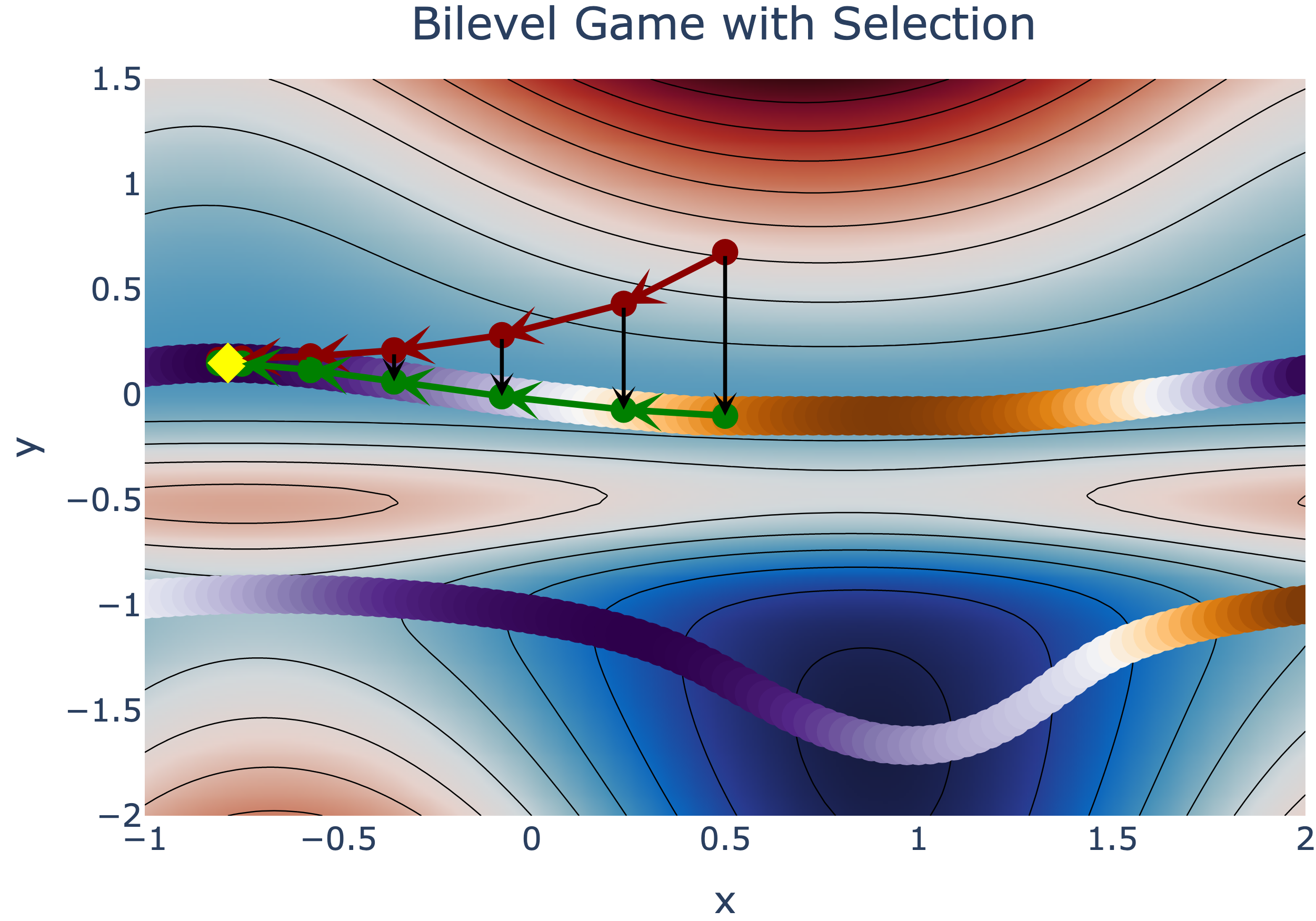
Figure 1: Left: Heatmap of the lower-level objective $g(x,y)$. The local minimizers of $y\mapsto g(x,y)$ are represented by the ’critical lines’ in blue. The selection map $\phi(x,y)$ is defined by following the vector field $\partial_{y}g(x,y)$, in black. Right: Iterates $(x_{k},y_{k})$ (in red) obtained by playing a BGS. The follower finds the next update $y_{k}$ by optimizing $y\mapsto g(x_{k},y)$ starting from previous iterate $y_{k-1}$. The leader finds the next update $x_{k}$ by optimizing the upper-level objective $f$ along the ’critical lines’ (iterates in green).

First-order equilibrium conditions.

The agents can play the game Equation BGS by successively taking actions $(x_{k},y_{k})$ to improve their own objectives $x\mapsto\mathcal{L}_{\phi}(x,y_{k-1})$ and $y\mapsto g(x_{k},y)$, by hoping the strategy will reach an equilibrium pair $(x^{*},y^{*})$ Figure 1(Right). In the case where $f$, $g$ and $\phi$ are differentiable at $(x^{*},y^{*})$, the equilibrium pair is characterized by a first-order stationary condition:

$$\partial_{x}\mathcal{L}_{\phi}(x^{\star},y^{\star})=\partial_{x}f(x^{\star},y^{\star})+\partial_{x}\phi(x^{\star},y^{\star})\partial_{y}f(x^{\star},y^{\star})=0,\qquad\partial_{y}g(x^{\star},y^{\star})=0.$$ (SC)

When $g$ is smooth and strongly convex in $y$, the implicit function theorem [28, Theorem 5.9] ensures that $\phi$ is differentiable and provides an expression of $\partial_{x}\phi(x^{\star},y^{\star})$ as a solution to a linear system which key for implicit differentiation. This allows to devise efficient algorithms using estimates of the gradient $\partial_{x}\mathcal{L}_{\phi}$, see, e.g., [2]. However, extensions of the implicit function theorem, such as the constant rank theorem  [29, Theorem 4.12], for cases where $g$ has possibly degenerate critical points require strong assumptions on $g$ which are unrealistic in machine learning. In the next section, we provide new analytical tools for extending implicit differentiation by studying the differentiability of a family of selection maps corresponding to a large class of functions $g$. The resulting expression will be key for devising first-order methods to solve Equation BGS, as discussed in Section 5.

4 Selection Based on Gradient Flows for Parameteric Morse-Bott Functions

In this section, we extend implicit differentiation to a class of functions with possibly degenerate critical points. To this end, we consider a particular selection $\phi(x,y)$ obtained as the limit of a gradient flow $(\phi_{t}(x,y))_{t\geq 0}$ of $g(x,.)$ initialized at $y$. We then study the differentiability w.r.t. $x$ of the selection by analyzing the dynamics of such a gradient flow. For general non-convex functions, the selection might be non-differentiable since a small perturbation to the parameter $x$ can change the geometry of the critical points of $g$, causing the perturbed flow to move away from the non-perturbed one (see Figure 2). We are therefore interested in functions $g$ preserving the local geometry near critical points as $x$ varies. In Section 4.1, we introduce such a class of functions called parametric Morse-Bott functions, which covers many practical machine learning models. We then show, in Section 4.2, that the selection resulting from such a function is differentiable near local minima.

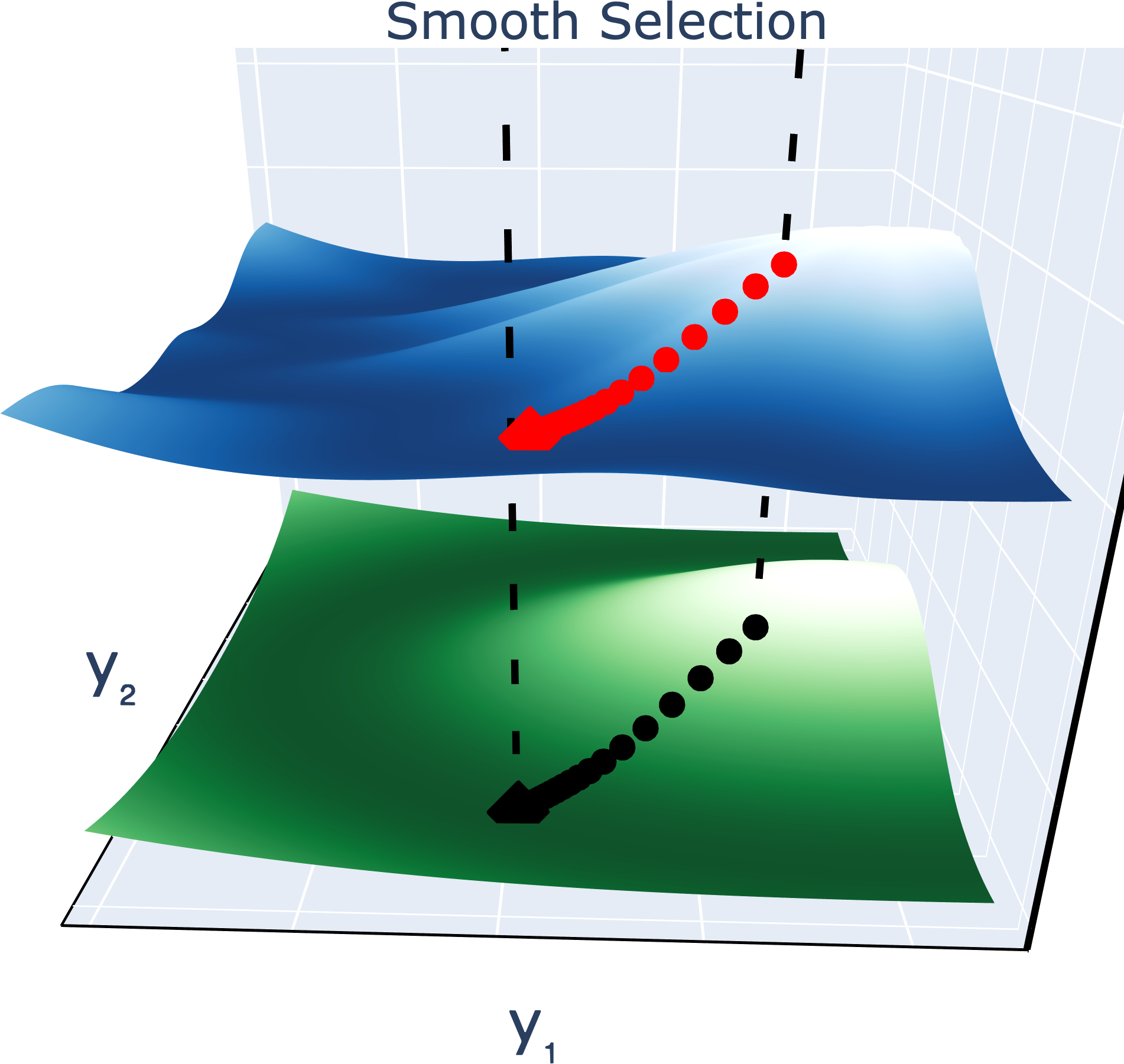
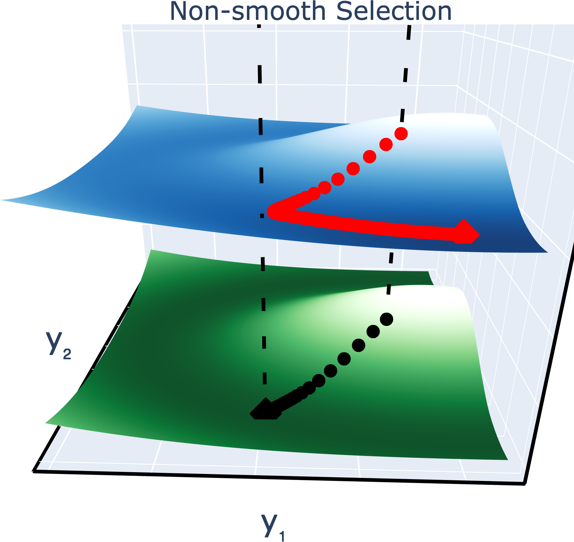
Figure 2: Two examples of functions $g$ with different behaviors of the gradient flow under perturbations of $x$. In both figures, the green surface represents a function $y\mapsto g(x_{0},y)$ with $y\in\mathbb{R}^{2}$ resembling a Mexican hat which has a manifold of (degenerate) local minimizers (in dark green). The blue surfaces represent deformed versions of the Mexican hat function when the parameter $x$ is slightly perturbed $x_{1}{\approx}x_{0}$. Depending on the deformation, the resulting function $y{\mapsto}g(x_{1},y)$ can either preserve the same type of critical points as the unperturbed function, i.e. local minimizers remain local minimizers (Left), or change their type, i.e.: local minimizers can become saddle-points (Right). Left: the selection behaves smoothly as a function of the deformation. Right: the selection is discontinuous since the gradient flow is pushed away from $\phi(x_{0},y_{0})$ which is deformed into a saddle point.

4.1 Parameteric Morse-Bott Functions

We introduce parametric Morse-Bott functions, a class of parametric functions $g:\mathcal{X}\times\mathcal{Y}\rightarrow\mathbb{R}$ with parameter $x$ in $\mathcal{X}$ extending the more familiar notion of Morse-Bott functions (Section A.1, [16]) to account for the effect of the parameter $x$ on the geometry of critical points.

Definition 2 (Parametric Morse-Bott function.).

Let $g:\mathcal{X}\times\mathcal{Y}$ be a real-valued twice continuousely differentiable function and define the set of augmented critical points $\mathcal{M}$ as follows:

$$\mathcal{M}:={\left\{(x,y)\in\mathcal{X}\times\mathcal{Y}\leavevmode\nobreak\ \middle|\leavevmode\nobreak\ \partial_{y}g(x,y)=0\right\}}$$ (1)

Let $(x_{0},y_{0})\in\mathcal{M}$. We say that $g$ is Morse-Bott at $y_{0}$ w.r.t. $x_{0}$, if there exists an open neighbordhood $\mathcal{V}$ of $(x_{0},y_{0})$ s.t. the intersection $\mathcal{M}\cap\mathcal{V}$ is a $C^{2}$-connected sub-manifold of $\mathcal{X}{\times}\mathcal{Y}$ of dimension:

$$\dim(\mathcal{M}\cap\mathcal{V})=\dim(\mathcal{X})+dim{\left(\text{Ker}(\partial^{2}_{yy}g(x_{0},y_{0}))\right)}.$$ (2)

$g$ is a parametric Morse-Bott function if for any $(x_{0},y_{0}){\in}\mathcal{M}$, $g$ is Morse-Bott at $y_{0}$ w.r.t. $x_{0}$.

The functions in 2 satisfy a condition that is stronger than simply satisfying the Morse-Bott property at any parameter value $x$ (3 of Section A.1). Indeed, we show in Proposition 7 of Section A.2 that, for any $x_{0}\in\mathcal{X}$, the function $y\mapsto g(x_{0},y)$ is a Morse-Bott function, meaning that the critical set $C(x_{0})$ of $y\mapsto g(x_{0},.)$ near a critical point $y_{0}$ is locally a $C^{2}$ connected sub-manifold of $\mathcal{Y}$ of dimension equal to the dimension of the null-space of the Hessian $\partial^{2}_{yy}g(x_{0},y_{0})$. For conciseness, we introduce the following assumption which ensures $g$ satisfies the condition of 2 as well as possesses continuous third-order derivatives.

Assumption 1 (Parameteric Morse-Bott property).

The function $g$ is at least three-times continuously differentiable and is a parameteric Morse-Bott function as defined in 2.

Examples of parametric Morse-Bott function.

A notable class of parametric Morse-Bott functions is the one containing all twice-continuously differentiable functions that are strongly convex or, more generally, possess only non-degenerate critical points in the second variable as shown in Proposition 8 of Section A.2. Note that parametric Morse-Bott functions need not be convex and can have multiple (possibly degenerate) local minima, saddle-points, and local maxima.

Another class of functions, this time with possibly degenerate critical points, are those that can be expressed as a composition of some Morse-Bott function $h$ and a family $(\tau_{x})_{x\in\mathcal{X}}$ of diffeomorphisms on $\mathcal{Y}$ parameterized by $x$, i.e. $g(x,y){=}h(\tau_{x}(y))$. This particular form is relevant in generative modeling where the diffeomorphisms are defined using normalizing flows of parameter $x$ [44].

The condition in 2 ensures that the degree of freedom of the augmented critical set $\mathcal{M}$ is exactly determined by the degree of freedom of the parameter $x$ and the degree of degeneracy of the Hessian at a critical point $y$. This condition is precisely what guarantees the stability of the local shape of critical points when the parameter $x$ varies as we formalize through the next theorem.

Theorem 1 (Morse-Bott lemma with parameters).

Let $g$ be a function satisfying Assumption 1. Let $(x_{0},y_{0})$ in $\mathcal{M}$ be an augmented critical point of $g$. Denote by $\mathcal{K}$ the null space of the Hessian $A_{0}{:=}\partial^{2}_{yy}g(x_{0},y_{0})$ and by $\mathcal{K}^{\perp}$ its orthogonal complement in $\mathcal{Y}$. Let $J_{0}$ be a diagonal matrix with diagonal element given by the sign of the non-zero eigenvalues of $A_{0}$. Then, there exists open neighborhoods $\mathcal{U}$ and $\mathcal{V}$ of $(x_{0},0_{\mathcal{K}},0_{\mathcal{K}^{\perp}})$ and $(x_{0},y_{0})$ in $\mathcal{X}{\times}\mathcal{K}{\times}\mathcal{K}^{\perp}$ and $\mathcal{X}{\times}\mathcal{Y}$, and a diffeomorphism $\psi:\mathcal{U}\rightarrow\mathcal{V}$ preserving the first variable, i.e. $\psi(x,r,w){=}(x,y)$ for any $(x,r,w)\in\mathcal{U}$, with $\psi(x_{0},0_{\mathcal{K}},0_{\mathcal{K}^{\perp}}){=}(x_{0},y_{0})$ such that $g$ admits the representation:

$$g(\psi(x,r,w))=g(\psi(x,0_{\mathcal{K}},0_{\mathcal{K}^{\perp}}))+\frac{1}{2}w^{\top}J_{0}w,\qquad\forall(x,r,w)\in\mathcal{U}.$$ (3)

Theorem 1, which is proven in Section A.3, shows that, near an augmented critical point $(x_{0},y_{0})$, $g$ looks like a quadratic function up to an additive term that depends only on the parameter $x$. Moreover, slightly varying the parameter $x$ does not change the quadratic function and thus preserves the local shape near critical points. Theorem 1 is an extension of the Morse-Bott lemma [16, Theorem 2.10] to the case when there is a dependence on a parameter $x$. It can also be seen as an extension of the Morse lemma with parameters [16, Theorem 4] which allows dependence to a parameter $x$ but requires the critical points to be non-degenerate (invertible matrix $A_{0}$). To our knowledge, Theorem 1 is the first result in the literature providing a decomposition of parametric functions with degenerate critical points into the sum of a quadratic non-degenerate term and a singular term depending only on the parameter $x$. We present now a corollary of Theorem 1 which is a strengthened version of the standard Łojasiewicz inequality [36] that will be essential for our subsequent analysis.

Proposition 1 (Locally Uniform Łojasiewicz gradient inequality).

Let $g$ be a function satisfying Assumption 1 and let $(x_{0},y_{0})$ be in $\mathcal{M}$ the augmented critical set defined in 2. Then, there exists an open neighborhood $\mathcal{U}$ of $(x_{0},y_{0})$ and a positive number $\mu>0$ such that $y\mapsto g(x,y)$ is constant on the set $\mathcal{M}\cap\mathcal{U}$ with some common value $G(x):=g(x,y)$ and the following holds:

$$\mu{\left\lvert g(x,y)-G(x)\right\rvert}\leq\frac{1}{2}{\left\lVert\partial_{y}g(x,y)\right\rVert}^{2},\qquad\forall(x,y)\in\mathcal{U}.$$ (4)

Proposition 1, which is proven in Section A.3, ensures that the Łojasiewicz gradient inequality holds uniformly on $(x,y)$ near any augmented critical point $(x_{0},y_{0})$. This result will be essential in Section 4.2 for defining a selection $\phi$ obtained as limits of gradient flows and to obtain a locally uniform control of these flows in the parameter $x$. This in turn will allow us to obtain the differentiability of the selection in the parameter $x$ whenever $\phi(x,y)$ is a local minimum.

4.2 Smoothness of Selections Based on Gradient Flows of a Parametric Morse-Bott Function

We consider a construction for the selection $\phi$ in 1 as a limit of a continuous-time gradient flow of $g$. More precisely, we define a continuous-time trajectory $(\phi_{t}(x,y))_{t\geq 0}$ in $\mathcal{Y}$ initialized at $\phi_{0}(x,y)=y$ and driven by the differential equation:

$$\frac{d\phi_{t}(x,y)}{dt}=-\partial_{y}g(x,\phi_{t}(x,y)).$$ (GF)

Provided $\phi_{t}(x,y)$ converges towards some element $\phi(x,y)$ as $t{\rightarrow}{+}\infty$, we can expect such a limit to satisfy both conditions of 1, therefore constituting a valid selection. However, for general non-convex functions, $\phi_{t}(x,y)$ might not always converge [36]. To guarantee the existence and convergence of the flow, we make the following assumptions on the function $g$.

Assumption 2 (Smoothness).

There exists $L{>}0$ such that $y{\mapsto}\partial_{y}g(x,y)$ is $L$-Lipschitz for any $x{\in}\mathcal{X}$.

Assumption 3 (Coercivity).

For any $x\in\mathcal{X}$, it holds that $g(x,y)\rightarrow+\infty$ as ${\left\lVert y\right\rVert}\rightarrow+\infty$.

The smoothness assumption in Assumption 2 is standard and guarantees the existence of the flow by the Cauchy-Lipschitz theorem. The coercivity condition in Assumption 3 guarantees that $\phi_{t}(x,y)$ cannot escape to infinity. It can be easily enforced by adding a small $\ell_{2}$-penalty to a non-negative loss (such as cross-entropy or mean-squared loss) which is already a common practice in machine learning. These assumptions, along with Assumption 1 ensure that the limit $\phi(x,y)$ always exists as we summarize in the following proposition, which is proven in Appendix B.

Proposition 2.

Under Assumptions 2, 1 and 3, and for any $(x,y)\in\mathcal{X}\times\mathcal{Y}$, the gradient flow Equation GF always converges towards a critical point $\phi(x,y)$ of $y\mapsto g(x,y)$ and the map $(x,y)\mapsto\phi(x,y)$ is a selection map as defined in 1. We call $\phi$ the flow selection relatively to $g$.

Proposition 2 is a consequence of a general result that holds for functions satisfying a Łojasiewicz gradient inequality [3, 40] which is the case here by Proposition 1. From now on, we restrict our attention to the selection $\phi$ defined in Proposition 2. Even though $\phi$ satisfies the implicit equation $\partial_{y}g(x,\phi(x,y))=0$, we cannot rely anymore on the implicit function theorem for studying the differentiability of $\phi(x,y)$ in $x$ since $g$ can have degenerate critical points. Instead, we propose to characterize the differentiability of $\phi$ by studying the limit of $U_{t}(x,y):=\partial_{x}\phi_{t}(x,y)$ which is formally driven by a linear differential equation of the form:

$$-\frac{dU_{t}(x,y)}{dt}=\partial^{2}_{xy}g(x,\phi_{t}(x,y))+U_{t}(x,y)\partial^{2}_{yy}g(x,\phi_{t}(x,y)).$$ (5)

Had we known in advance that $\phi(x,y)$ is differentiable in $x$, the limit $U_{\infty}(x,y)$ of $U_{t}(x,y)$ as $t\rightarrow+\infty$, whenever defined, would be a promising candidate for the differential of $\phi(x,y)$ in $x$. Such a limit is indeed expected to satisfy the following linear equation:

$$0=\partial^{2}_{xy}g(x,\phi(x,y))+U_{\infty}(x,y)\partial^{2}_{yy}g(x,\phi(x,y)).$$ (6)

A first challenge is to ensure that $U_{t}$ does not diverge. For critical points $\phi(x,y)$ that are not local minima, it is easy to see that the Hessian $\partial^{2}_{yy}g(x,\phi_{t}(x,y))$ must have a negative eigenvalue for $t$ large enough, therefore causing the system Equation 5 to diverge. Intuitively, unless $\phi(x,y)$ is a local minimum, there is no reason to expect $\phi(x,y)$ to be differentiable or even continuous in $x$, simply because $\phi(x,y)$ would be an unstable fixed-point of the flow $\phi_{t}(x,y)$, so that any change in $x$ might cause a large variation in $\phi(x,y)$. The possible non-differentiability of $\phi(x,y)$ for critical points that are not local minima is not problematic in practice, since for almost all initial conditions $y$ of the flow $\phi_{t}(x,y)$, the limit $\phi(x,y)$ is guaranteed to be a local minimizer [41]. In addition, we show in Proposition 13 of Section B.3 that if $\phi(x_{0},y)$ is a local minimum, then $\phi(x,y)$ must also be a local minimum in a neighborhood of $x_{0}$.

Nevertheless, even for local minima, if the Hessian $\partial^{2}_{yy}g(x,\phi(x,y))$ is non-invertible, Equation 6 might never hold if $\partial^{2}_{xy}g(x,\phi(x,y))$ does not belong to the image of the Hessian. However, we show in Proposition 6 of Section A.2 that, for any pair $(x,y)$ of critical points, $\partial^{2}_{xy}g(x,y)$ must always belong to the span of the Hessian $\partial^{2}_{yy}g(x,y)$ as soon as $g$ satisfies Assumption 1, therefore ensuring that Equation 6 admits a solution. The following theorem, which is proven in Appendix C, establishes the differentiability of $\phi$ at local minima and shows that $\partial_{x}\phi$ is exactly given by the limit $U_{\infty}$.

Theorem 2 (Differentiability of the flow selection).

Let $g$ be a function satisfying Assumptions 3, 1 and 2 so that the flow selection $\phi$ is well-defined. Let $(x_{0},y_{0})$ be in $\mathcal{X}{\times}\mathcal{Y}$. If $\phi(x_{0},y_{0})$ is a local minimizer of $y\mapsto g(x_{0},y)$, then there exists a neighborhood $\mathcal{U}$ of $x_{0}$ on which $x\mapsto\phi(x,y_{0})$ is differentiable with differential $\partial_{x}\phi(x,y_{0}){=}U_{\infty}(x,y_{0})$. Moreover, if $y_{0}$ is a local minimizer of $y{\mapsto}g(x_{0},y)$, then, denoting by $\dagger$ the pseudo inverse operator, $\partial_{x}\phi(x_{0},y_{0})$ is exactly given by:

$$\partial_{x}\phi(x_{0},y_{0}){=}-\partial_{xy}g(x_{0},y_{0}){\left(\partial_{yy}g(x_{0},y_{0})\right)}^{\dagger}.$$ (7)

The expression in Equation 7 is very similar to the one that would arise by application of the implicit function theorem to a strongly convex function $g$. However, the proof technique does not rely on such a theorem which would not be applicable here. The key technical challenges in proving the above result are: (i) showing that $\phi(x,y)$ must be continuous at $x_{0}$ and (ii) controlling the error ${\left\lVert U_{t}(x,y)-U_{\infty}(x,y)\right\rVert}$ locally uniformly in $x$. The result follows by the application of classical uniform convergence results [46, Theorem 7.17]. The continuity of $\phi$ is established in Proposition 12 of Section B.3 and relies on a stability analysis of the flow $\phi_{t}$ performed in Section B.2. The uniform convergence of $U_{t}$ towards $U_{\infty}$ is shown in Proposition 17 of Appendix C and relies on a local uniform convergence of the flow $\phi_{t}$ towards $\phi$ which is proven in Proposition 14 of Section B.4. It is worth noting that, even though we identified $\partial_{x}\phi$ to be $U_{\infty}$, the latter is not fully characterized by Equation 6 as it might contain a non-zero component in the null-space of the Hessian. However, when $(x_{0},y_{0})$ is an augmented critical pair of $g$, such a component vanishes, and $\partial_{x}\phi(x_{0},y_{0})$ is exactly determined by the minimal norm solution in Equation 7. The latter fact has practical implications when designing algorithms for solving Equation BGS as we discuss next.

5 Algorithms

5.1 Unrolled Optimization for BGS

Unrolled optimization constructs a map $\varphi_{T}(x,y)$ approximating a critical point of the function $y\mapsto g(x,y)$ for any fixed $x$ by applying a finite number $T>0$ of gradient updates starting from some initial condition $y$. By convention, we set $\varphi_{0}(x,y){=}y$. Hence, $\varphi_{T}$ can be understood as an approximation to the selection map defined in Section 4.2. We emphasize that $\varphi_{T}$ is not a selection (1) since $\varphi_{T}(x,y)$ is not a critical point of $g$ in general. Nevertheless, it provides a tractable approximation to critical points which is key for constructing practical algorithms for bilevel optimization. The gradient of $\varphi_{T}(x,y)$ w.r.t. $x$ is then obtained by differentiating through the optimization steps and used to optimize the approximate upper-level objective:

$$\mathcal{L}_{T}(x,y):=f(x,\varphi_{T}(x,y)).$$ (8)

Given the $k$-th upper-level iterate $x_{k}$ and an initial condition $\tilde{y}_{k}$ for the unrolled optimization, these approaches compute an approximation $y_{k}{=}\varphi_{T}({x_{k\text{--}1}},\tilde{y}_{k})$ and find an update direction $d_{k}$ for the upper-level variable $x$ by differentiating $\mathcal{L}_{T}(x,\tilde{y}_{k})$ in $x$ at the current iterate ${x_{k\text{--}1}}$. The following iterate $x_{k}$ is obtained by applying an update procedure, such as $x_{k}{=}{x_{k\text{--}1}}{-}\gamma d_{k}$ for positive small enough step-size $\gamma$. In Algorithm 1, we present several variants of these schemes, including a simple correction allowing them to solve Equation BGS instead of an approximation.

The initial condition $\tilde{y}_{k}$ is often computed using a warm-start procedure $\tilde{y}_{k}{=}\mathcal{I}_{M}({x_{k\text{--}1}},{y_{k\text{--}1}})$. The simplest procedure is to set $\tilde{y}_{k}{=}{y_{k\text{--}1}}$ in which case $\mathcal{I}_{0}(x,y){=}y$. However, it is not uncommon to perform $M{>}0$ optimization steps to minimize the objective $y{\mapsto}g({x_{k\text{--}1}},y)$ starting from ${y_{k\text{--}1}}$. By doing so, gradient unrolling stops at $\tilde{y}_{k}$ and ignores the dependence of $\tilde{y}_{k}$ on ${y_{k\text{--}1}}$, resulting in Truncated unrolled optimization [47]. Algorithm 1 summarizes these approaches when the binary variable AddCorrection is set to False. To characterize the limit points of Algorithm 1, we make the following assumptions on $\mathcal{I}_{M}$, $\mathcal{\varphi}_{T}$.

Algorithm 1 BGS-Opt$(x_{0},y_{0})$

1:  Inputs: $x_{0}$, $y_{0}$,

2:  Parameters: $K$, $T$, $M$ , $\gamma$ AddCorrection

3:  for  $k\in\{1,...,K+1\}$  do

4:     $\tilde{y}_{k}\leftarrow\mathcal{I}_{M}{\left({x_{k\text{--}1}},{y_{k\text{--}1}}\right)}$. # Warm-start.

5:     $y_{k}{\leftarrow}\varphi_{T}{\left({x_{k\text{--}1}},\tilde{y}_{k}\right)}$ # Unrolled optimization.

6:     $d_{k}\leftarrow\partial_{x}\mathcal{L}_{T}{\left({x_{k\text{--}1}},\tilde{y}_{k}\right)}$

7:     if AddCorrection$=$ True  then

8:        $v_{k}\leftarrow\partial_{y}\mathcal{L}_{T}{\left({x_{k\text{--}1}},\tilde{y}_{k}\right)}$

9:        $\xi_{k}{\approx}-{\left(\partial_{yy}g({x_{k\text{--}1}},y_{k})\right)}^{\dagger}v_{k}$ # Approx. solver

10:        $d_{k}\leftarrow d_{k}+{\color[rgb]{0,0,0}\partial_{xy}g({x_{k\text{--}1}},y_{k})\xi_{k}}$ # Grad. correction

11:     end if

12:     $x_{k}\leftarrow{x_{k\text{--}1}}-\gamma d_{k}$ # Updating $x$

13:  end for

14:  Return $(x_{K},y_{K})$.

Assumption 4.

For any non-negative integers $M,T\geq 0$, the maps $\mathcal{I}_{M}$ and $\mathcal{\varphi}_{T}$ are continuous on $\mathcal{X}\times\mathcal{Y}$ and take values in $\mathcal{Y}$, with $\varphi_{T}$ being continuously differentiable. Moreover, for any $(x,y)\in\mathcal{X}\times\mathcal{Y}$ s.t. $\partial_{y}g(x,y){=}0$ and $M,T\geq 0$, there exists a matrix $D$ such that:

$$\mathcal{I}_{M}(x,y)=\varphi_{T}(x,y)=y,\quad\partial_{x}\varphi_{T}(x,y)=\partial^{2}_{xy}g(x,y)D,\quad\partial_{y}\varphi_{T}(x,y)=I+\partial^{2}_{yy}g(x,y)D.$$ (9)

Finally, for any $(x,y){\in}\mathcal{X}{\times}\mathcal{Y}$, and $M,T\geq 0$ s.t. $T+M>0$, the equality $y{=}\varphi_{T}(x,\mathcal{I}_{M}(x,y))$ implies that $y$ is a critical point of $g$, i.e. $\partial_{y}g(x,y)=0$.

Assumption 5.

$\varphi_{T}$ converges to a selection $\phi$ and $\partial_{x}\varphi_{T}$ converges uniformly near local minima.

Assumption 4 is satisfied by many mappings used in practice such as $T$-steps of the gradient descent or proximal point algorithms, whenever $g$ is twice-continuousely differentiable and $L$-smooth as shown in Proposition 19 of Appendix D. Assumption 5 is a discrete-time version of the uniform convergence result in Proposition 17 of Appendix C but that we directly assume here for simplicity. Under these assumptions we show that Algorithm 1 can find equilibria of Equation BGS up to an approximation error resulting from the fact that $\varphi_{T}$ is not an exact selection.

Proposition 3.

Let $M,T$ be non-negative numbers s.t. $M+T>0$ and let $(x_{k},y_{k})$ be the iterates of Algorithm 1 using the maps $\mathcal{I}_{M}$ and $\varphi_{T}$ and without any correction, i.e. AddCorrection${=}$False. If $(x_{k},y_{k})$ converges to a limit point $(x_{T}^{\star},y_{T}^{\star})$ then, under Assumption 4:

$$\partial_{x}\mathcal{L}_{T}(x_{T}^{\star},y_{T}^{\star})=0,\qquad\partial_{y}g(x_{T}^{\star},y_{T}^{\star})=0.$$ (10)

Let $E$ be the set of limit points $(x_{T}^{\star},y_{T}^{\star})$ for $T\geq 0$. If $E$ is bounded and $y_{T}^{\star}$ is a local minimum of $g(x_{T}^{\star},.)$ for any $T\geq 0$, then, under Assumptions 4 and 5, the elements of $E$ are approximate equilibria for Equation BGS:

$$\lim\sup_{T}{\left\lVert\partial_{x}\mathcal{L}_{\phi}(x_{T}^{\star},y_{T}^{\star})\right\rVert}=0,\qquad\partial_{y}g(x_{T}^{\star},y_{T}^{\star})=0,\quad(\forall T>0).$$ (11)

Proposition 3 shows that unrolled optimization algorithms approximately solve Equation BGS in the limit where the number of unrolling steps $T$ of the $\varphi_{T}$ goes to infinity. This result is consistent with the ones obtained in [25] for the case where $g$ is strongly convex and illustrates the high computational cost for solving Equation BGS without correcting for the bias introduced by unrolling. Next, we show how to get rid of such a bias in light of Theorem 2.

5.2 Implicit Gradient Correction

We propose to correct the bias of unrolling by exploiting the expression of the gradient $\partial_{x}\phi$ provided in Theorem 2. The key idea is to obtain an expression for $\partial_{x}\mathcal{L}_{\phi}(x,y)$ in terms of $\mathcal{L}_{T}$ and the second-order derivatives of $g$ which holds for any local minimizer $y$ of $y\mapsto g(x,y)$ as shown by the proposition below.

Proposition 4.

Let $\phi$ be the selection defined in Section 4.2 and $(x,y)\in\mathcal{X}\times\mathcal{Y}$ be s.t. $y$ is a local minimum of $y\mapsto g(x,y)$. Then, under Assumptions 3, 4, 1 and 2, $\partial_{x}\mathcal{L}_{\phi}(x,y)$ is given by the equation:

$$\partial_{x}\mathcal{L}_{\phi}(x,y):=\partial_{x}\mathcal{L}_{T}(x,y)-\partial^{2}_{xy}g(x,y){\left(\partial^{2}_{yy}g(x,y)\right)}^{\dagger}\partial_{y}\mathcal{L}_{T}(x,y).$$ (12)

Proposition 4, which is proven in Appendix D, suggests a simple correction for the gradient estimate $d_{k}$ in Algorithm 1. By doing so, the corrected algorithm would be performing an approximate gradient descent on each of the upper-level and lower-level objectives, suggesting that the algorithm may recover equilibrium points of Equation BGS without having to increase the computation budget for the unrolling as we show later in Proposition 5. A simple way to proceed would to compute $c_{k}$ satisfying the approximate equation $c_{k}{\approx}-B_{k}(A_{k})^{\dagger}v_{k}$, where $A_{k}{=}\partial^{2}_{yy}g({x_{k\text{--}1}},y_{k})$, $B_{k}{:=}\partial^{2}_{xy}g({x_{k\text{--}1}},y_{k})$ and $v_{k}{=}\partial_{y}\mathcal{L}_{T}({x_{k\text{--}1}},\tilde{y}_{k})$. More concretely, $c_{k}$ can be computed by setting $c_{k}{=}B_{k}\xi_{k}$ where $\xi_{k}$ approximates the minimum norm solution to the least squares problem:

$$\xi_{k}\approx\arg\min_{\xi}{\left\lVert\xi\right\rVert}^{2},\qquad s.t.\quad\xi\in\arg\min_{\xi}{\left\lVert A_{k}\xi+v_{k}\right\rVert}^{2},$$ (13)

Approximate solution to Equation 13. It is possible to solve Equation 13 approximately using an iterative procedure by constructing $N$ iterates $\xi^{t}$ starting from $\xi^{0}=0$ and performing (conjugate) gradient descent on the quadratic objective. This can be implemented efficiently using only Hessian vector products with the Hessian $A_{k}$ [37]. The constrained problem Equation 13 can also be expressed as an unconstrained one by re-parametrizing $\xi=A_{k}z$:

$$\xi_{k}\approx A_{k}z_{k}^{\star},\qquad s.t.\quad z_{k}^{\star}\in\arg\min_{z}{\left\lVert A_{k}^{2}z+v_{k}\right\rVert}^{2}.$$ (14)

Eq. Equation 14 has the advantage that $z_{k}^{\star}$ solves an unconstrained problem. As such, it is more amenable to applying a warm-start strategy, which can yield efficient approximation $z_{k}$ to $z_{k}^{\star}$ by exploiting previously computed approximation $z_{k-1}$ to $z_{k-1}^{\star}$  [2]. This strategy can be achieved using a standard iterative algorithm $\mathcal{P}$ for approximately solving the least-squares problems, such as a fixed number of conjugate gradient iterations, that takes as input the matrix $A_{k}$, vector $v_{k}$ and initialization $z_{k-1}\approx z_{k-1}^{\star}$ and returns the next iterate $z_{k}\approx z_{k}^{\star}$. More formally we view $\mathcal{P}$ as a continuous map of $(A,v,z)\mapsto\mathcal{P}(A,v,z)$ returning a vector $z^{\prime}$ and such that the only fixed points are exact solutions to the least square problem $\min_{z}{\left\lVert A^{2}z+v\right\rVert}^{2}$. We refer to Section D.1 for examples of such maps. We can then define the iterates $z_{k}$ and $\xi_{k}$ as follows:

$$\xi_{k}=A_{k}z_{k},\qquad z_{k}=\mathcal{P}(A_{k},v_{k},z_{k-1}).$$ (15)

The corrected algorithm is obtained by setting the variable AddCorrection${=}$True in Algorithm 1 and computing the $\xi_{k}$ using any approximate solver including, in particular, the ones based on a warm-start strategy as in Equation 15. The following proposition, with proof in Appendix D, shows that the proposed correction indeed yields equilibrium points of Equation BGS.

Proposition 5.

Let $(x_{k},y_{k})$ be the iterates obtained using Algorithm 1 with AddCorrection${=}$True and $T+M>0$ and assume that $\xi_{k}$ are computed using Equation 15. If $(x_{k},y_{k},z_{k})_{k\geq 0}$ converges to a limit point $(x^{\star},y^{\star},z^{\star})$, then $y^{\star}$ is a critical point of $y\mapsto g(x^{\star},y)$ and if, in addition, $y^{\star}$ is a local minimizer, then $(x^{*},y^{*})$ must be an equilibrium of Equation BGS satisfying Equation SC:

$$\partial_{x}\mathcal{L}_{\mathcal{\phi}}(x^{\star},y^{\star})=0\leavevmode\nobreak\ \leavevmode\nobreak\ \leavevmode\nobreak\ \leavevmode\nobreak\ \text{and}\leavevmode\nobreak\ \leavevmode\nobreak\ \leavevmode\nobreak\ \leavevmode\nobreak\ \partial_{y}g(x^{\star},y^{\star})=0$$ (16)

Proposition 5 shows that the proposed correction allows to recover equilibria of Equation BGS without having to increase the number of iterations $T$ of the unrolled algorithm. This is by contrast with Proposition 3 where $T$ must increase to infinity, which would be impractical. We discuss in Section D.2 how different choices for the parameters $T$ and $M$ recover known algorithms. In particular, that Algorithm 1 with correction allows interpolating between two families of algorithms: (ITD) and (AID) while still recovering the correct equilibria. Numerical results illustrating the benefits of the correction are presented in Appendix E.

6 Discussion

We have introduced a bilevel game that resolves the ambiguity in bilevel optimization with non-convex objectives using the notion of selection maps. We have shown that many algorithms for bilevel optimization approximately solve these games up to a bias due to finite computational power. Our study of the differentiability properties of the selection maps has resulted in practical procedures for correcting such a bias and required the development of new analytical tools. This study opens the way for several avenues of research to understand the tradeoff between unrolling and implicit gradient correction for designing efficient algorithms. In future work, studying these algorithms in a non-smooth and stochastic setting would also be of great theoretical and practical interest.

Funding

This project was supported by ANR 3IA MIAI@Grenoble Alpes (ANR-19-P3IA-0003).

Checklist

The checklist follows the references. Please read the checklist guidelines carefully for information on how to answer these questions. For each question, change the default [TODO] to [Yes] , [No] , or [N/A] . You are strongly encouraged to include a justification to your answer, either by referencing the appropriate section of your paper or providing a brief inline description. Please do not modify the questions and only use the provided macros for your answers. Note that the Checklist section does not count towards the page limit. In your paper, please delete this instructions block and only keep the Checklist section heading above along with the questions/answers below.

1. For all authors…

   1. Do the main claims made in the abstract and introduction accurately reflect the paper’s contributions and scope? [Yes]

   2. Did you describe the limitations of your work? [Yes]

   3. Did you discuss any potential negative societal impacts of your work? [N/A]

   4. Have you read the ethics review guidelines and ensured that your paper conforms to them? [Yes]

2. If you are including theoretical results…

   1. Did you state the full set of assumptions of all theoretical results? [Yes]

   2. Did you include complete proofs of all theoretical results? [Yes]

3. If you ran experiments…

   1. Did you include the code, data, and instructions needed to reproduce the main experimental results (either in the supplemental material or as a URL)? [N/A]

   2. Did you specify all the training details (e.g., data splits, hyperparameters, how they were chosen)? [N/A]

   3. Did you report error bars (e.g., with respect to the random seed after running experiments multiple times)? [N/A]

   4. Did you include the total amount of compute and the type of resources used (e.g., type of GPUs, internal cluster, or cloud provider)? [N/A]

4. If you are using existing assets (e.g., code, data, models) or curating/releasing new assets…

   1. If your work uses existing assets, did you cite the creators? [N/A]

   2. Did you mention the license of the assets? [N/A]

   3. Did you include any new assets either in the supplemental material or as a URL? [N/A]

   4. Did you discuss whether and how consent was obtained from people whose data you’re using/curating? [N/A]

   5. Did you discuss whether the data you are using/curating contains personally identifiable information or offensive content? [N/A]

5. If you used crowdsourcing or conducted research with human subjects…

   1. Did you include the full text of instructions given to participants and screenshots, if applicable? [N/A]

   2. Did you describe any potential participant risks, with links to Institutional Review Board (IRB) approvals, if applicable? [N/A]

   3. Did you include the estimated hourly wage paid to participants and the total amount spent on participant compensation? [N/A]

Appendix A Morse-Bott Lemma with Parameters

A.1 Background on Morse-Bott Functions

We recall the definition of classical Morse-Bott functions [4, 16], which we extend in Section 4.1 to the case where there is a dependence on some additional parameter $x$ in $\mathcal{X}$.

Definition 3 (Morse-Bott function).

Let $h:\mathcal{Y}\rightarrow\mathbb{R}$ be a real-valued twice continuousely differentiable function. Define $\mathcal{C}_{h}$ to be the set of critical points of $h$ and consider $y_{0}\in C_{h}$. We say that $h$ is Morse-Bott at $y_{0}$, if there exists a open neighbordhood $\mathcal{V}$ of $y_{0}$ such that $C_{h}\cap\mathcal{V}$ is a connected sub-manifold of $\mathcal{Y}$ of dimension $\dim{\left(\text{Ker}(\partial_{yy}^{2}h(y_{0}))\right)}$. We say that $h$ is a Morse-Bott function if for any $y_{0}\in\mathcal{C}_{h}$, $h$ is Morse-Bott at $y_{0}$.

Morse-Bott functions were introduced in the context of differential topology to analyze the geometry of a manifold by studying the properties of differentiable functions defined on that manifold [4]. Their main property is that all their critical points that are connected have the same type (same number of positive and negative eigenvalues for the Hessian), a fact expressed by the Morse-Bott lemma [16, Theorem 2.10] that we generalize to the parametric setting in Theorem 1. Morse-Bott functions form a generic class of functions [39], meaning that any smooth function can always be slightly perturbed to become a smooth Morse-Bott function. Hence, in principle, requiring that $y\mapsto g(x,y)$ is a Morse-Bott function for any parameter $x\in\mathcal{X}$ is essentially a mild assumption. The Morse-Bott property allows characterizing the geometry of critical points of $g(x,.)$ for any $x$ and ensures that the selection map $\phi$ is well-defined [11, Chapter 15]. However, this condition does not provide any information about how the set of critical points evolves as the parameter $x$ varies, which is crucial for the study of smoothness of the selection $\phi$. This is precisely why we introduced parametric Morse-Bott functions in Section 4.1.

A.2 Properties of Parameteric Morse-Bott Functions.

In this section, we describe some elementary properties of parametric Morse-Bott functions. In particular, Proposition 6 shows that $\partial_{xy}^{2}g(x,y)$ belongs to the range of $\partial_{yy}^{2}g(x,y)$ whenever $(x,y)$ is an augmented critical point of $g$, i.e. $\partial_{y}g(x,y)=0$. Proposition 7 shows that any parametric Morse-Bott function $g$ satisfies a pointwise Morse-Bott property in the sense of 3. Finally, Propositions 8 and 1 provide examples of functions that satisfy the parametric Morse-Bott property. Recall $\mathcal{M}$ the set of augmented critical points of $g$:

$$\mathcal{M}={\left\{(x,y)\in\mathcal{X}\times\mathcal{Y}\middle|\partial_{y}g(x,y)=0\right\}}.$$ (17)

Proposition 6 (Exact least square solution).

Let $g$ be a parametric Morse-Bott function. Let $(x_{0},y_{0})$ be an element in $\mathcal{M}$ defined in Equation 17 and define the matrices $A:=\partial_{yy}^{2}g(x_{0},y_{0})$ and $B:=\partial_{xy}^{2}g(x_{0},y_{0})$. Then, $B$ is in the range of $A$, i.e. there exists a matrix $U$ such that $B{=}UA$.

Proof.

Recall that $\mathcal{M}$ is the set of augmented critical points of $g$. Since $g$ is a parametric Morse-Bott function, there exists a neighborhood $\mathcal{U}$ of $(x_{0},y_{0})$ such that the augmented critical set $\mathcal{M}\cap\mathcal{U}$ is a $C^{2}$ manifold of dimension $d_{\mathcal{M}}{=}\dim(\mathcal{X})+\dim(Ker(\partial_{yy}^{2}g(x_{0},y_{0})))$. We know that $\mathcal{M}\cap\mathcal{U}$ is characterized locally by the equation $\partial_{y}g(x_{0},y_{0})=0$, hence the tangent space $T{\mathcal{M}}_{(x_{0},y_{0})}$ of $\mathcal{M}\cap\mathcal{U}$ at point $(x_{0},y_{0})$ consist of the set of directions $(u,v)\in\mathcal{X}\times\mathcal{Y}$ for which $\partial_{y}g(x_{0}+\epsilon u,y_{0}+\epsilon v)=O(\epsilon^{2})$. In other words $T{\mathcal{M}}_{(x_{0},y_{0})}$ is the set of vectors $(u,v)\in\mathcal{X}\times\mathcal{Y}$ of $\mathcal{M}\cap\mathcal{U}$ satisfying the equation:

$$u^{\top}\partial_{xy}^{2}g(x_{0},y_{0})+v^{\top}\partial_{yy}^{2}g(x_{0},y_{0}){=}u^{\top}B+v^{\top}A{=}0.$$ (18)

Since $\mathcal{M}\cap\mathcal{U}$ is of dimension $d_{\mathcal{M}}$, the tangent space $T\mathcal{M}_{(x_{0},y_{0})}$ must also have dimension $d_{\mathcal{M}}$. Therefore, by the rank theorem, it must hold that the matrix $D=(B,A)$ has a rank equal to $\dim(\mathcal{X})+\dim(\mathcal{Y})-d_{\mathcal{M}}=\text{rank}(A)$. On the other hand, we know that $0^{\top}B+v^{\top}A=v^{\top}A\in Range(A)$ for any $v\in\mathcal{Y}$, so that $Range(A)\subset Range(D)$. The two subspaces having the same dimension, the inclusion implies equality ($Range(A)=Range(D)$). Henceforth, there must exist a matrix $U$ such that $B$ can be written as $B{=}UA$. ∎

Proposition 7 (Pointwise Morse-Bott property).

Let $g$ be a parametric Morse-Bott function. Then for any $x\in\mathcal{X}$, the function $y\mapsto g(x,y)$ is a Morse-Bott function in the following sense: For any $x_{0}$ and any critical point $y_{0}$ of $g(x_{0},.)$, there exists an open neighborhood $\mathcal{V}$ of $y_{0}$ so that $C_{x,y_{0}}:={\left\{y\in\mathcal{Y}\middle|\partial_{y}g(x_{0},y)=0\right\}}\cap\mathcal{V}$ is a connected sub-manifold of dimension equal to the dimension of the null space of the Hessian $\partial_{yy}^{2}g(x,y_{0})$.

Proof.

Let $(x_{0},y_{0})$ be in $\mathcal{X}\times\mathcal{Y}$ such that $\partial_{y}g(x_{0},y_{0})=0$. Then, since $g$ is a parameteric Morse-Bott function, there exists a neighborhood $\mathcal{U}$ of $(x_{0},y_{0})$ such that the augmented critical set $\mathcal{M}\cap\mathcal{U}$ is a $C^{2}$ manifold of dimension $d_{\mathcal{M}}{=}\dim(\mathcal{X})+\dim(Ker(\partial_{yy}^{2}g(x_{0},y_{0})))$. On the other hand, we know that $\mathcal{M}\cap\mathcal{U}$ is characterized locally by the equation $\partial_{y}g(x,y)=0$, hence the tangent vectors $(u,v)\in\mathcal{X}\times\mathcal{Y}$ of $\mathcal{M}\cap\mathcal{U}$ at $(x_{0},y_{0})$ must satisfy the equation:

$$u^{\top}\partial_{xy}^{2}g(x_{0},y_{0})+v^{\top}\partial_{yy}^{2}g(x_{0},y_{0}){=}0.$$ (19)

For simplicity, we denote by $B=\partial_{xy}^{2}g(x_{0},y_{0})$ and $A=\partial_{yy}^{2}g(x_{0},y_{0})$. By Proposition 6, we know that $B$ can be written in the form $B=UA$ for some matrix. Hence, the tangent space of $\mathcal{M}$ at $(x_{0},y_{0})$ consists in vectors $(u,v)\in\mathcal{X}\times\mathcal{Y}$ satisfying

$${\left(u^{\top}U+v\right)}A=0.$$ (20)

In particular, for any $u\in\mathcal{X}$, we can set $v=-u^{\top}U$ which ensures that $(u,v)$ is in the tangent space of $\mathcal{M}$ at $(x_{0},y_{0})$. Now consider the sub-manifold $\{x_{0}\}\times\mathcal{Y}$, its tangent space at $(x_{0},y_{0})$ is $\{0\}\times\mathcal{Y}$. For any element $(x,y)\in\mathcal{X}\times\mathcal{Y}$, we have the decomposition $(x,y){=}(x,-x^{\top}U)+(0,y+x^{\top}U)$ where the first tuple belongs to the tangent space of $\mathcal{M}$ and the second one belongs to the tangent space of $\{x_{0}\}\times\mathcal{Y}$ at $(x_{0},y_{0})$. Hence, the tangent space of $\mathcal{X}\times\mathcal{Y}$ is generated by the both separate tangent spaces which means that both manifolds intersect transversally and that $\{x_{0}\}\times\mathcal{C}:=(\mathcal{M}\cap\mathcal{U})\cap(\{x_{0}\}\times\mathcal{Y})$ is a sub-manifold of dimension $\dim{\left(Ker{\left(\partial_{yy}^{2}g(x_{0},y_{0})\right)}\right)}$ [29, Theorem 6.30]. For a small enough open connected neighborhood $\mathcal{V}$ of $y_{0}$, we can ensure that $\mathcal{C}\cap\mathcal{V}$ is a connected sub-manifold of $\mathcal{Y}$. This precisely means that $y\mapsto g(x_{0},y)$ is Morse-Bott at the point $y_{0}$ which concludes the proof. ∎

Proposition 8 (Morse functions with parameters).

Let $g:\mathcal{X}\times\mathcal{Y}$ be a three-times continuously differentiable function such that for any $(x,y)\in\mathcal{X}\times\mathcal{Y}$ for which $\partial_{y}g(x,y)=0$, the Hessian matrix $\partial_{yy}^{2}g(x,y)$ is invertible. Then $g$ is a parametric Morse-Bott function.

Proof.

Let $(x_{0},y_{0})\in\mathcal{X}\times\mathcal{Y}$ be such that $y_{0}$ is a critical point of $g(x_{0},.)$ ( i.e. $\partial_{y}g(x_{0},y_{0}){=}0$). Since, by assumption, the Hessian is invertible, we can apply the implicit function theorem which guarantees the existence of a function $x\mapsto y(x)$ defined in a neighborhood $\mathcal{U}$ of $x_{0}$ and taking values in a neighborhood $\mathcal{V}$ of $y_{0}$, such that $y(x_{0})=y_{0}$ and $y(x)$ is the unique critical point of $g(x,.)$ on $\mathcal{V}$, i.e.:

$$\partial_{y}g(x,y(x))=0,\qquad\forall x\in\mathcal{U}.$$ (21)

Moreover, $x\mapsto y(x)$ is twice continuously differentiable. This ensures that $\mathcal{M}$ the set of augmented critical points of $g$ satisfies:

$$\mathcal{M}\cap{\left(\mathcal{U}\times\mathcal{V}\right)}={\left\{(x,y(x))\in\mathcal{X}\times\mathcal{Y}\middle|x\in\mathcal{U}\right\}}:=\mathcal{S}.$$ (22)

We only need to show that $\mathcal{M}\cap{\left(\mathcal{U}\times\mathcal{V}\right)}$ is a manifold of dimension $\dim(\mathcal{X})$. For this, we will apply the regular level set theorem  [29, Corollary 5.14] to the function $G:(x,y)\mapsto\partial_{y}g(x,y)$ defined on $\mathcal{U}\times\mathcal{V}$. The pre-image of $0$ by $G$ is exactly equal to $\mathcal{M}\cap{\left(\mathcal{U}\times\mathcal{V}\right)}$. Moreover, for any $(x,y)\in\mathcal{M}\cap{\left(\mathcal{U}\times\mathcal{V}\right)}$, we have that $dG(x,y)$ is of maximal rank since $\partial_{yy}^{2}g(x,y)$ is invertible. Hence, by application of the regular level set theorem theorem to the twice continuously differentiable ($C^{2}$) function $G$, it follows that $\mathcal{M}\cap{\left(\mathcal{U}\times\mathcal{V}\right)}=G^{-1}({\left\{0\right\}})$ is a $C^{2}$ sub-manifold of $\mathcal{X}\times\mathcal{Y}$ of dimension $\dim(ker(dG(x,y)))=\dim(\mathcal{X})$. We have shown that $\mathcal{M}\cap{\left(\mathcal{U}\times\mathcal{V}\right)}$ is sub-manifold of dimension $\dim(\mathcal{X})$, which proves the result. ∎

Lemma 1.

Let $h$ be a smooth Morse-Bott function defined on $\mathcal{Y}$. Let $\mathcal{T}:\mathcal{X}\times\mathcal{Y}\rightarrow\mathcal{Y}$ be a smooth function, such that $y\mapsto\mathcal{T}(x,y)=\tau_{x}(y)$ is a diffeomorphism on $\mathcal{Y}$ for any $x\in\mathcal{X}$. Then the function $g(x,y)=h(\tau_{x}(y))$ is a parametric Morse-Bott function.

Proof.

Consider the function $G:(x,y)\mapsto\partial_{y}g(x,y)$. We have the following equivalence

$$(x,y)\in G^{-1}({\left\{0\right\}})\iff\partial_{y}h(\tau_{x}(h))\partial_{y}\tau_{x}(y)=0\iff\tau_{x}(y)\in\partial_{y}h^{-1}({\left\{0\right\}}).$$ (23)

Consider the map $\mathcal{T}:(x,y)\mapsto\tau_{x}(y)$, then we have shown that $G^{-1}({\left\{0\right\}})=\mathcal{T}^{-1}{\left(\partial_{y}h^{-1}({\left\{0\right\}})\right)}$. Let $(x_{0},y_{0})\in\mathcal{X}\times\mathcal{Y}$ be an augmented critical point of $g$. Set $\tilde{y}=\mathcal{T}(x_{0},y_{0})$ which is a critical point of $h$. Since $h$ is, by assumption, Morse-Bott at $\tilde{y}$, then there exists an open neighborhood $\tilde{\mathcal{V}}$ of $\tilde{y}$ such that $\partial_{y}h^{-1}({\left\{0\right\}})\cap\tilde{\mathcal{V}}$ is a sub-manifold of dimension $\dim(Ker(\partial_{yy}^{2}h(\tilde{y})))$. By continuity of $\mathcal{T}$, we can always find open connected neighborhoods $\mathcal{U}$ and $\mathcal{V}$ of $(x_{0},y_{0})$ so that $\mathcal{V}^{\prime}{:=}\mathcal{T}(\mathcal{U}\times\mathcal{V})\subset\tilde{\mathcal{V}}$. Moreover, since for any $x$ $\mathcal{T}(x,.)$ is a diffeomorphism, it must be that $\mathcal{V}^{\prime}$ is an open set. Therefore, $\mathcal{S}:=\partial_{y}h^{-1}({\left\{0\right\}})\cap\mathcal{V}^{\prime}$ must be a sub-manifold as of dimension $\dim(Ker(\partial_{yy}^{2}h(\tilde{y})))$. It remains to show that $\mathcal{T}^{-1}(\mathcal{S})$ is a sub-manifold. To see this, it suffice to note that the differential of $\mathcal{T}$ is surjective which ensures that $\mathcal{T}$ is transverse to $\mathcal{S}$ and that $\mathcal{T}^{-1}(\mathcal{S})$ is a sub-manifold [29, Theorem 6.30]. Moreover, the dimension of such manifold is equal to $\dim(\mathcal{X})+\dim(ker(\partial_{yy}^{2}h(\tilde{y})))=\dim(\mathcal{X})+\dim(ker(\partial_{yy}^{2}g(x_{0},y_{0})))$.

∎

A.3 Proof of the Morse-Bott Lemma with Parameters

In this section, we provide a proof of the Morse-Bott lemma with parameters introduced in Theorem 1. We then introduces two results in Propositions 9 and 1 which are consequences of Theorem 1. Proposition 9 shows that near an augmented critical point $(x_{0},y_{0})$, the Hessian matrices of nearby augmented critical points are all similar. This result illustrates that the geometry near a critical point is preserved when the parameter $x$ is perturbed. Proposition 9 will be used later in Proposition 16 of Appendix C to show that the pseudo-inverse of the Hessian matrices of critical points near a local minimum are uniformly bounded. Finally, Corollary 1 shows that near any augmented critical point $(x_{0},y_{0})$ the function $y\mapsto g(x,y)$ can be expressed as a slight deformation of $y\mapsto g(x_{0},y)$. This result, along with the stability result in Section B.2 of the gradient flow to deformations will be key to prove the continuity of the selection map $x\mapsto\phi(x,y)$ near local minima.

Proof of Theorem 1.

Let $x_{0}\in\mathcal{X}$ and $y_{0}$ be a critical point of $g(x_{0},.)$. Denote by $\mathcal{K}$ the null space of the Hessian $A_{0}=\partial_{yy}^{2}g(x_{0},y_{0})$ and by $\mathcal{K}^{\perp}$ its orthogonal complement in $\mathcal{Y}$. The function $g(x_{0},.)$ is a Morse-Bott function by Proposition 7, therefore by the Morse-Bott lemma [16, Theorem 2.10], there exists three open neighborhoods $\mathcal{O}$, $\mathcal{O}^{\perp}$ and $\mathcal{V}$ of $0\in\mathcal{K}$, $0\in\mathcal{K}^{\perp}$ and $y_{0}\in\mathcal{Y}$ and a diffeomorphism $s:\mathcal{O}\times\mathcal{O}^{\perp}\rightarrow\mathcal{V}$ s.t. $s(0,0)=y_{0}$ and for any $r,w\in\mathcal{O}\times\mathcal{O}^{\perp}$ it holds that:

$$g(x_{0},s(r,w))=g(x_{0},y_{0})+\frac{1}{2}w^{\top}J_{0}w,\forall r,w\in\mathcal{O}\times\mathcal{O}^{\perp}.$$ (24)

where $J_{0}$ is an invertible diagonal matrix whose diagonal elements are equal to the sign of the non-zero eigenvalues of the Hessian $\partial_{yy}^{2}g(x_{0},y_{0})$. By convention $J_{0}{=}0$ in case the Hessian $\partial_{yy}^{2}g(x_{0},y_{0})=0$. Since, the function $h(x,r,w):=g(x,s(r,w))$ is such that $\partial_{w}h(x_{0},0,0)=0$ and the partial Hessian $\partial_{ww}^{2}h(x_{0},0,0)=J_{0}$ is invertible, we are in position to apply the Morse lemma with parameters [16, Theorem 4]. The lemma ensures that $\mathcal{O}$ and $\mathcal{O}^{\perp}$ can be chosen small enough so that there exits open neighborhoods $\mathcal{B}$ and $\mathcal{O}^{\perp}_{1}$ of $x_{0}\in\mathcal{X}$ and $0\in\mathcal{K}^{\perp}$ and a diffeomorphism $\tau$ from $\mathcal{B}\times\mathcal{O}\times\mathcal{O}_{1}^{\perp}$ to $\mathcal{B}\times\mathcal{O}\times\mathcal{O}^{\perp}$ such that $\tau(x_{0},0,0){=}(x_{0},0,0)$ and decomposing $h$ locally into a quadratic component and a singular one. More precisely, for any $(x,r,w)\in\mathcal{B}\times\mathcal{O}\times\mathcal{O}_{1}^{\perp}$, the map $r$ satisfies $\tau(x,r,w){=}(x,r,w^{\prime})$ for some $w^{\prime}\in\mathcal{O}^{\perp}$ and the following equation holds:

$$h(\tau(x,r,w))=h(\tau(x,r,0))+\frac{1}{2}w^{\top}J_{0}w.$$ (25)

It remains to show that $\xi\mapsto h(\tau(x,r,0))$ is in fact constant for $(x,r)$ in an open neighborhood of $(x_{0},0)\in\mathcal{X}\times\mathcal{O}$. To this end, define the sets $A$, $B$ and $C$ as follows:

$$A :={\left\{(x,y)\in\mathcal{B}\times\mathcal{V}\quad\middle|\quad\partial_{y}g(x,y)=0\right\}},$$ (26)

$$B :={\left\{(x,r,w)\quad\middle|\quad(x,r)\in\mathcal{B}\times\mathcal{O},\quad\partial_{r}h(\tau(x,r,w))=0\right\}},$$ (27)

$$C :={\left\{(x,r,0)\quad\middle|\quad(x,r)\in\mathcal{B}\times\mathcal{O},\quad\partial_{r}h(\tau(x,r,0))=0\right\}}.$$ (28)

Then by Equation 25, it holds that $B=C$. Moreover, $A$ and $B$ are homeomorphic. Indeed to see this, we introduce the notation $\tilde{s}(x,r,w):=(x,s(r,w))$ which defines a diffeomorphism from $\mathcal{B}\times\mathcal{O}\times\mathcal{O}^{\perp}$ to $\mathcal{B}\times\mathcal{V}$. Hence, $g\circ\tilde{s}\circ\tau=h\circ\tau$. This ensures $\tilde{s}\circ\tau(B){=}A$, which means precisely that $A$ and $B$ are homeomorphic since $\tilde{s}\circ\tau$ is a homeomorphism. Moreover, by definition of $g$ as a parametric Morse-Bott function, we also know that $A$ is a sub-manifold of $\mathcal{X}\times\mathcal{Y}$ of dimension $\dim(\mathcal{X})+\dim{\left(Ker{\left(\partial_{yy}^{2}g(x_{0},y_{0})\right)}\right)}$ provided the neighborhoods $\mathcal{B}$ and $\mathcal{V}$ are small enough. Hence, we can deduce that $B$ and $C$ must also be sub-manifolds of the same dimension. In particular, $C$ is a sub-manifold of $\mathcal{B}\times\mathcal{O}\times\{0\}$ which is of dimension $\dim(\mathcal{X})+\dim{\left(Ker{\left(\partial_{yy}^{2}g(x_{0},y_{0})\right)}\right)}$. Therefore, $C$ is an open sub-manifold of $\mathcal{B}\times\mathcal{O}\times\{0\}$. Hence, since $(x_{0},0,0)\in C$, there must exists an open connected neighborhood $\mathcal{B}_{1}\times\mathcal{O}_{1}\times\{0\}$ of $(x_{0},0,0)$ in $\mathcal{B}\times\mathcal{O}\times\{0\}$ that is contained in $C$. Hence, we deduce that for any $(x,r)\in\mathcal{B}_{1}\times\mathcal{O}_{1}$, the function $h$ satisfies $\partial_{r}h(\tau(x,r,0))=0$ so that $h(\tau(x,r,0))=h(\tau(x,0,0))$ on such neighborhood. Finally, we have shown that there exits

$$g\circ\tilde{s}\circ\tau(x,r,w)=g\circ\tilde{s}\circ\tau(x,0,0)+\frac{1}{2}w^{\top}J_{0}w.$$

We conclude the proof by setting $\psi(x,r,w)=\tilde{s}\circ\tau(x,r,w)$ which is the desired diffeomorphism. ∎

Proposition 9.

Let $g$ be a real-valued function such that Assumption 1 holds. Consider an augmented critical point $(x_{0},y_{0}){\in}\mathcal{M}$, with $\mathcal{M}$ defined in Equation 17. Then there exists a neighborhood $\mathcal{V}$ of $(x_{0},y_{0})$ and a continuous map $(x,y)\mapsto P(x,y)$ defined on $\mathcal{V}$ with values in $\mathbb{R}^{d\times d}$ such that:

• $P(x,y)$ is invertible for any $(x,y)\in\mathcal{V}$ with singular values contained in an interval $[\sigma_{\min},\sigma_{\max}]$ for some positive constants $\sigma_{\min}$ and $\sigma_{\max}$.

• For any augmented critical point $(x,y)\in\mathcal{V}$, the Hessian of $g$ is given by:

  $$\partial_{yy}^{2}g(x,y)=P(x,y)^{\top}\partial_{yy}^{2}g(x_{0},y_{0})P(x,y).$$

Proof.

Denote by $\mathcal{K}$ the null space of the Hessian $A_{0}=\partial_{yy}^{2}g(x_{0},y_{0})$ and by $\mathcal{K}^{\perp}$ its orthogonal complement in $\mathcal{Y}$. Let $J_{0}$ be a diagonal matrix with diagonal elements given by the sign of the non-zero eigenvalues of $A_{0}$. Since $g$ satisfies Assumption 1, we apply Theorem 1 which ensures the existence of a diffeomorphism $\psi$ defined on an open neighborhood $\mathcal{U}$ of $(x_{0},0,0)\in\mathcal{X}\times\mathcal{K}\times\mathcal{K}^{\perp}$ with values in an open neighborhood $\mathcal{V}$ of $(x_{0},y_{0})$ in $\mathcal{X}\times\mathcal{Y}$, s.t. $\psi(x_{0},0,0)=(x_{0},y_{0})$ and for all $(x,r,w)\in\mathcal{U}$, $\psi$ satisfies $\psi(x,r,w){=}(x,y)$ and

$$g(\psi(x,r,w)) =g(\psi(x,0,0))+\frac{1}{2}w^{\top}J_{0}w,$$ (29)

$$=g(\psi(x,0,0))+\frac{1}{2}(r^{\top}w^{\top})\tilde{J}_{0}\begin{pmatrix}r\\ w\end{pmatrix},$$ (30)

where we defined $\tilde{J}_{0}$ to be the matrix of dimension $d\times d$ given by:

$$\tilde{J}_{0}=\begin{pmatrix}0&0\\ 0&J_{0}\end{pmatrix}.$$ (31)

Since $\psi$ is a diffeomorphism satisfying $\psi(x,r,w)=(x,y)$, we can equivalently write Equation 29 as:

$$g(x,y)=g(\psi(x,0,0))+\frac{1}{2}\psi^{-1}_{2,3}(x,y)^{\top}\tilde{J}_{0}\psi^{-1}_{2,3}(x,y),\qquad\forall(x,y)\in\mathcal{V},$$ (32)

where $\psi_{2,3}^{-1}(x,y)$ are last two components of $\psi^{-1}(x,y)$ (i.e. $\psi^{-1}(x,y)=(x,\psi_{2,3}^{1}(x,y))$). By differentiating Equation 32 w.r.t. $y$ we obtain:

$$\partial_{y}g(x,y)=\partial_{y}\psi^{-1}_{2,3}(x,y)\tilde{J}_{0}\psi^{-1}_{2,3}(x,y).$$ (33)

$\partial_{y}\psi^{-1}_{2,3}(x,y)$ must be invertible since $(\partial_{x}\psi^{-1},\partial_{y}\psi^{-1})$ is invertible and of the form:

$$\begin{pmatrix}\partial_{x}\psi^{-1}\\ \partial_{y}\psi^{-1}\end{pmatrix}=\begin{pmatrix}I&\partial_{x}\psi_{2,3}^{-1}\\ 0&\partial_{y}\psi_{2,3}^{-1}\end{pmatrix}.$$ (34)

Therefore, if $y$ is a critical point of $g(x,.)$, then Equation 33 implies that $\tilde{J}_{0}\psi^{-1}_{2,3}(x,y)=0$. Let $(x,y)$ be an augmented critical point of $g$, $\epsilon>0$ and $u$ be vector in $\mathcal{Y}$, then the following holds:

$$\frac{1}{\epsilon}\partial_{y}g(x,y+\epsilon u)={\left(\partial_{y}\psi_{2,3}^{-1}(x,y+\epsilon u)\right)}^{\top}\tilde{J}_{0}{\left(\frac{1}{\epsilon}\psi_{3}^{-1}(x,y+\epsilon u)-\psi_{2,3}^{-1}(x,y)\right)}.$$ (35)

Hence, by taking the limit when $\epsilon$ approaches $0$, it follows that:

$$\partial_{yy}^{2}g(x,y)={\left(\partial_{y}\psi_{2,3}^{-1}(x,y)\right)}^{\top}\tilde{J}_{0}\partial_{y}\psi_{2,3}^{-1}(x,y).$$ (36)

Define $P_{0}:=\partial_{y}\psi_{2,3}^{-1}(x_{0},y_{0})\partial_{y}\psi_{2,3}^{-1}(x_{0},y_{0})^{\top}$ which is invertible. Then, we can write:

$$\partial_{yy}^{2}g(x,y) =\partial_{y}\psi_{2,3}^{-1}(x,y)^{\top}P_{0}^{-1}P_{0}\tilde{J}_{0}P_{0}P_{0}^{-1}\partial_{y}\psi_{2,3}^{-1}(x,y)$$ (37)

$$=\partial_{y}\psi_{2,3}^{-1}(x,y)^{\top}P_{0}^{-1}\partial_{y}\psi_{2,3}^{-1}(x_{0},y_{0})A_{0}\partial_{y}\psi_{2,3}^{-1}(x_{0},y_{0})^{\top}P_{0}^{-1}\partial_{y}\psi_{2,3}^{-1}(x,y)$$ (38)

$$=P(x,y)^{\top}\partial_{yy}^{2}g(x_{0},y_{0})P(x,y),$$ (39)

where we defined $P(x,y){=}\partial_{y}\psi_{2,3}^{-1}(x_{0},y_{0})^{\top}P_{0}^{-1}\partial_{y}\psi_{2,3}^{-1}(x,y)$. The matrix $P(x,y)$ is invertible for any $(x,y)\in\mathcal{V}$ and the map $(x,y)\mapsto P(x,y)$ is continuous. Hence, by considering compact neighborhood of $(x_{0},y_{0})$ contained in $\mathcal{V}$, we can ensure that the singular values of $P(x,y)$ are contained in an interval $[\sigma_{\min},\sigma_{\max}]$ where $\sigma_{\min}$ and $\sigma_{\max}$ are positive numbers. Further considering the restriction of such map on an open neighborhood $\mathcal{V}^{\prime}\subset K$ of $(x_{0},y_{0})$ yields the desired result. ∎

Corollary 1.

Let $g$ be a real-valued function such that Assumption 1 holds. Consider an augmented critical point $(x_{0},y_{0}){\in}\mathcal{M}$, with $\mathcal{M}$ defined in Equation 17. Then, there exists a open neighborhoods $\mathcal{B}$ and $\mathcal{V}$ of $x_{0}$ and $y_{0}$ in $\mathcal{X}$ and $\mathcal{Y}$ and a continuously differentiable map $\tau$ from $\mathcal{B}\times\mathcal{V}$ to $\mathcal{V}$ such that:

• For any $x\in\mathcal{B}$, the map $\tau_{x}:y\mapsto\tau(x,y)$ is a diffeomorphism from $\mathcal{V}$ to itself satisfying $\tau_{x_{0}}(y)=y$ for any $y\in\mathcal{V}$. Moreover, $(x,y)\mapsto\tau_{x}^{-1}(y)$ is continuous.

• For any $(x,y)\in\mathcal{B}\times\mathcal{V}$, the function $g$ satisfies $g(x,y){=}g(x_{0},\tau(x,y))+C(x)$, where $x\mapsto C(x)$ is a function independent of $y$.

• There exists positive numbers $\ell$ and $L$ s.t for any $(x,y)\in\mathcal{B}\times\mathcal{V}$:

  $$\ell^{2}I\leq\partial_{y}\tau(x,y)^{\top}\partial_{y}\tau(x,y)\leq(L^{\prime})^{2}I.$$ (40)

Proof.

We use the notations of Theorem 1 where $\mathcal{K}$ is the null subspace of the Hessian $\partial_{yy}^{2}g(x_{0},y_{0})$ and $\mathcal{K}^{\perp}$ its orthogonal complement in $\mathcal{Y}$. By Theorem 1 $g$ satisfies:

$$g(\psi(x,r,w))=g(\psi(x,0,0))+\frac{1}{2}\bar{y}^{\top}J_{0}\bar{y},$$ (41)

with $\psi$ and $J_{0}$ being the diffeomorphism and matrix defined in Theorem 1. Recall that $\psi$ is defined on an open neighborhood $\mathcal{B}\times\mathcal{O}\times\mathcal{O}^{\perp}$ of $(x_{0},0,0)\in\mathcal{X}\times\mathcal{K}\times\mathcal{K}^{\perp}$ and whose image by $\psi$ is an open neighborhood $\mathcal{B}\times\mathcal{V}$ of $(x_{0},y_{0})$. Hence, we can write:

$$g(\psi(x,r,w))=C(x)+g(\psi(x_{0},r,w)),$$

with $C(x):=g(\psi(x,0,0))-g(\psi(x_{0},0,0))$. We also know that $\psi$ preserves $x$, meaning that $\psi(x,r,w){=}(x,y)$. Hence, we can define $(x,r,w)\mapsto\tilde{\tau}_{x}(r,w)\in\mathcal{Y}$, s.t. $\psi(x,r,w){=}(x,\tilde{\tau}_{x}(r,w))$. For any $x\in\mathcal{B}$, $(r,w)\mapsto\tilde{\tau}_{x}(r,w)$ defines a diffeomorphism from $\mathcal{O}\times\mathcal{O}^{\perp}$ onto its image. Moreover, its image must be equal to $\mathcal{V}$. Indeed, since $\psi(\mathcal{B}\times\mathcal{O}\times\mathcal{O}^{\perp})=\mathcal{B}\times\mathcal{V}$, it follows that for any $(x,y)\in\mathcal{B}\times\mathcal{V}$, there exists $(r,w)\in\mathcal{O}\times\mathcal{O}^{\perp}$ such that $\psi(x,r,w)=(x,\tilde{\tau}_{x}(r,w))=(x,y)$. In particular, if $(x,y)\in\mathcal{B}\times\mathcal{V}$ and $(r,w)=\tilde{\tau}_{x}^{-1}(y)$, we can write $\psi(x_{0},r,w){=}(x_{0},\tilde{\tau}_{x_{0}}(r,w)){=}(x_{0},\tilde{\tau}_{x_{0}}\tilde{\tau}_{x}^{-1}(y))$. Therefore, the following expression holds for any $(x,y)\in\mathcal{B}\times\mathcal{V}$:

$$g(x,y)=C(x)+g(x_{0},\tau(x,y)),$$

where we defined $\tau(x,y){=}\tilde{\tau}_{x_{0}}\circ\tilde{\tau}_{x}^{-1}(y)$. For any $x\in\mathcal{B}$, the map $\tau_{x}:y\mapsto\tau(x,y)$ is a diffeomorphism satisfying $\tau(x_{0},y){=}y$. Moreover, $(x,r,w)\mapsto\tilde{\tau}_{x}(r,w)$ and $(x,y)\mapsto\tilde{\tau}_{x}^{-1}(y)$ are continuously differentiable since $\psi$ is a diffeomorphism. As a result, $\tau$ is continuously differentiable as well and $(x,y)\mapsto\tau_{x}^{-1}(y)$ is continuously differentiable. Finally, since $\partial_{y}\tau(x,y)$ is jointly continuous in $x$ and $y$ and $\partial_{y}\psi_{x}(y)$ is invertible, then, provided that $\mathcal{B}$ and $\mathcal{V}$ are small enough, there must exist two positive numbers $\ell$ and $L^{\prime}$ such that for any $(x,y)\in\mathcal{B}\times\mathcal{V}$:

$$\ell^{2}I\leq\partial_{y}\psi(y)^{\top}\partial_{y}\psi(y)\leq(L^{\prime})^{2}I.$$ (42)

∎

Proof of Proposition 1 .

Recall $\mathcal{M}={\left\{(x,y)\in\mathcal{X}\times\mathcal{Y}\middle|\partial_{y}g(x,y)=0\right\}}$ the set of augmented critical points of $g$ and let $(x_{0},y_{0})$ be in $\mathcal{M}$. First, since Assumption 1 holds, we know by Proposition 7 that $g(x_{0},.)$ is a Morse-Bott function. Hence, by [16, Theorem 1], it follows that $g(x_{0},.)$ satisfies a Łojasiewicz inequality near $y_{0}$. In other words, there exists a neighborhood $\mathcal{V}$ of $y_{0}$ and a positive constant $\mu^{\prime}>0$ such that:

$$\mu^{\prime}{\left\lvert g(x_{0},y)-g(x_{0},y_{0})\right\rvert}\leq\frac{1}{2}{\left\lVert\partial_{y}g(x_{0},y)\right\rVert}^{2},\qquad\forall y\in\mathcal{V}.$$ (43)

By Corollary 1, there exists a continuous function $\tau$ defined on an open neighborhood $\mathcal{B}\times\mathcal{V}$ of $(x_{0},y_{0})$ whose image is $\mathcal{V}$ and for which $g(x,y){=}g(x_{0},\tau(x,y)){+}C(x)$ for any $(x,y)\in\mathcal{B}\times\mathcal{V}$, where $C(x)$ is a function of $x$ independent of $y$. Moreover, for any $x\in\mathcal{B}$, $y\mapsto\tau(x,y)$ is a diffeomorphism from $\mathcal{V}$ to itself whose inverse is written as $\tau^{-1}(x,y)$ by an abuse of notion. In particular, for $y{=}\tau^{-1}(x,y_{0})$ we set $G(x){:=}g(x,\tau^{-1}(x,y_{0}))=g(x_{0},y_{0})+C(x)$. Note that $\tau^{-1}(x,y_{0})$ is critical point of $g(x,.)$ since $\partial_{y}g(x,\tau^{-1}(x,y_{0}))\partial_{y}\tau^{-1}(x,y_{0}){=}\partial_{y}g(x_{0},y_{0})=0$ and $\partial_{y}\tau^{-1}(x,y_{0})$ is invertible. Hence, the following holds for any $(x,y)\in\mathcal{B}\times\mathcal{V}$.

$$\mu^{\prime}{\left\lvert g(x,y)-G(x)\right\rvert}=\mu^{\prime}{\left\lvert g(x_{0},\tau(x,y))-g(x_{0},y_{0})\right\rvert}\leq\frac{1}{2}{\left\lVert\partial_{y}g(x_{0},\tau(x,y)\right\rVert}^{2}.$$ (44)

Moreover, by construction of $\tau$, we know that $\partial_{y}\tau(x,y)$ satisfies Equation 40 for any $(x,y)\in\mathcal{B}\times\mathcal{V}$. Therefore, we deduce that:

$${\left\lVert\partial_{y}g(x,y)\right\rVert}^{2}={\left\lVert\partial_{y}g(x_{0},\tau(x,y))\partial_{y}\tau(x,y)\right\rVert}^{2}\geq\ell^{2}{\left\lVert\partial_{y}g(x_{0},\tau(x,y))\right\rVert}^{2},$$ (45)

Finally, combining the above inequality with Equation 44, we get that, for any $(x,y)\in\mathcal{B}\times\mathcal{V}$:

$$\ell^{2}\mu^{\prime}{\left\lvert g(x,y)-G(x)\right\rvert}\leq\frac{1}{2}{\left\lVert\partial_{y}g(x,y)\right\rVert}^{2},\qquad\forall(x,y)\in\mathcal{U}.$$ (46)

The result follows by setting $\mu=\ell^{2}\mu^{\prime}>0$ and $\mathcal{U}=\mathcal{B}\times\mathcal{V}$. ∎

Appendix B Asymptotic Properties of Gradient Flows

B.1 Convergence of the gradient flow.

Recall that the gradient flow $\phi_{t}(x,y)$ satisfies the differential equation

$$\frac{d\phi_{t}(x,y)}{dt}=-\partial_{y}g(x,\phi_{t}(x,y)),\quad\phi_{0}(x,y)=y.$$

The next proposition shows that the gradient flow $\phi_{t}(x,y)$ converges towards a well-defined selection map $\phi(x,y)$.

Proposition 10 (Convergence of $\phi_{t}$.).

Let $x,y$ be in $\mathcal{X}\times\mathcal{Y}$. Under Assumptions 1, 2 and 3, $(t,x,y)\mapsto\phi_{t}(x,y)$ is continuous and for any $(x,y)\in\mathcal{X}\times\mathcal{Y}$, $\phi_{t}(x,y)$ converges towards a unique critical point $\phi(x,y)$ of $y\mapsto g(x,y)$ as $t$ goes to $+\infty$.

Proof.

First, Assumption 2 ensures that the gradient flow $\phi_{t}(x,y)$ is uniquely defined at all times $t$ [12]. $\phi_{t}(x,y)$ is jointly continuous in $(t,x,y)$ by Cauchy-Lipschitz theorem. Moreover, $t\mapsto\phi_{t}(x,y)$ remains bounded thanks to Assumption 3. Otherwise, there exists a subsequence $\phi_{t_{n}}(x,y)$ such that $g(x,\phi_{t_{n}}(x,y))$ diverges to $+\infty$. This contradicts the fact that $g(x,\phi_{t_{n}}(x,y))$ is decreasing since $\phi_{t}(x,y)$ is a gradient flow of $g$. Hence, we deduce that $\phi_{t}(x,y)$ must have at least one accumulation point $y^{\star}$. Moreover, $y^{\star}$ must be a critical point of $g(x,.)$. To see this, note that $g(x,\phi_{t}(x,y))$ is a decreasing function in time and is lower-bounded. Hence, it admits a finite limit $l$. Moreover, by differentiating $g(x,\phi_{t}(x,y))$ is time, it follows that:

$$\frac{\mathop{}\!\mathrm{d}}{\mathop{}\!\mathrm{d}t}g(x,\phi_{t}(x,y))=-{\left\lVert\partial_{y}g(x,\phi_{t}(x,y))\right\rVert}^{2}$$ (47)

This implies that $\int_{0}^{+\infty}{\left\lVert\partial_{y}g(x,\phi_{s}(x,y))\right\rVert}^{2}\mathop{}\!\mathrm{d}s=g(x,y)-l$ is finite. Since, $g$ is $L$-smooth by Assumption 2, this is only possible if $\partial_{y}g(x,\phi_{s}(x,y))$ converges to $0$. In particular, by continuity of $\partial_{y}g(x,y)$, it follows that $\partial_{y}g(x,y^{\star})=0$. We only need to show that $y^{\star}$ is the unique accumulation point of $\phi_{t}(x,y)$. To show this, we apply Proposition 1, which implies, in particular, that $g$ satisfies a Łojasiewicz inequality in a neighborhood $\mathcal{V}$ of $y^{\star}$:

$$\mu{\left\lvert g(x,y)-G(x)\right\rvert}\leq{\left\lVert\partial_{y}g(x,y)\right\rVert}^{2},\forall y\in\mathcal{V}.$$ (48)

We can therefore apply [40, Theorem 2.7] which ensure that $y^{\star}$ is the unique accumulation point of $\phi_{t}(x,y)$ and that $\phi_{t}(x,y)$ converges towards $y^{\star}$. We can therefore defined the map $\phi(x,y)=\lim_{t\rightarrow\infty}\phi_{t}(x,y)$ which constitues a selection.

∎

B.2 Stability of the Gradient Flow Near Local Minima

In this section, we provide a general result establishing the stability of gradient flows to perturbations. This result shows that deforming a gradient flow by a family of diffeomorphisms yields trajectories that are not too far from the unperturbed flow. We will use this result later in Section B.3 in conjunction with the formulation of $y\mapsto g(x,y)$ as a perturbation of $y\mapsto g(x_{0},y)$ provided in Corollary 1 to prove that the gradient flow $\phi_{t}(x,y)$ remain stable as the parameter $x$ varies.

Proposition 11 (Stability near local minima).

Let $h$ be a real valued differentiable function defined on $\mathcal{Y}$ and $y_{0}$ be a local minimizer of $h$. We assume that $h$ satisfies the Łojasiewicz inequality near $y_{0}$, meaning that there exists $\mu>0$ and $R>0$ s.t.:

$$\mu(h(y)-h(y_{0}))\leq\frac{1}{2}{\left\lVert\partial_{y}h(y)\right\rVert}^{2},\qquad\forall y\in B(y_{0},R).$$ (49)

Let $\mathcal{V}$ be an open neighborhood of $y_{0}$, $R^{\prime}>0$ such that $B(y_{0},2R^{\prime})\subset\mathcal{V}$ and $\mathcal{P}$ a family of diffeomorphisms defined from $\mathcal{V}$ to itself and satisfying:

1. For any $\tau{\in}\mathcal{P}$, the pre-image $y_{\psi}{:=}\psi^{-1}(y_{0})$ of $y_{0}$ by $\psi$ belongs to $B(y_{0},R^{\prime})$.

2. There exists positive numbers $\ell$ and $L^{\prime}$ s.t. for any $\tau\in\mathcal{P}$ and any $y\in\mathcal{V}$:

   $$\ell^{2}I\leq\partial_{y}\tau(y)^{\top}\partial_{y}\tau(y)\leq(L^{\prime})^{2}I.$$ (50)

For some $\tau\in\mathcal{P}$, consider a maximal solution $(z_{t})$ of the following ODE:

$$\dot{z_{t}}=-\partial_{y}h(\tau(z_{t}))\partial_{z}\tau(z_{t}),\qquad z_{0}\in B{\left(y_{\tau},R^{\prime}\right)}.$$ (51)

Then, there exists $0<C\leq R^{\prime}$, such that for any $0<\epsilon\leq C$, there exists $0<\eta\leq\frac{\epsilon}{2}$ with the following property:

For any $\tau\in\mathcal{P}$ and any $z_{0}$ s.t. ${\left\lVert z_{0}-y_{\tau}\right\rVert}\leq\eta$:

1. The solution $z_{t}$ to Equation 51 is well-defined at all times $t\geq 0$.

2. For all $t\geq 0$, it holds that ${\left\lVert z_{t}-y_{\tau}\right\rVert}\leq\epsilon$.

Proof.

The proof is inspired from the the abstract stability result in [31]. We know that $y_{0}$ is a local minimizer of $h$, therefore there exists $R">0$ such that for any $y$ satisfying ${\left\lVert y-y_{0}\right\rVert}\leq R"$, it holds that $\mathcal{L}(y):=h(y)-h(y_{0})\geq 0$. Moreover, by Equation 49, we also have that:

$$2\mu\mathcal{L}(y)\leq{\left\lVert\partial_{y}\mathcal{L}(y)\right\rVert}^{2},\qquad\forall y\in B(y_{0},R).$$ (52)

Take $\epsilon<\frac{1}{L^{\prime}}\min(R,R",L^{\prime}R^{\prime}):=C$. To simplify subsequent calculations, we will choose $y$ close enough to $y_{0}$ so that $2\ell^{-1}\sqrt{\frac{2}{\mu}}\mathcal{L}(y)^{\frac{1}{2}}\leq\epsilon$, where $\mu$ is the positive constant appearing in Equation 56 and $\ell$ is the positive constant in Equation 50. This is possible by continuity of $\mathcal{L}$ which that there exists $0<\eta\leq\frac{\epsilon}{2}$ for which any $y\in B(y_{0},L^{\prime}\eta)$ satisfies:

$$\mathcal{L}(y)^{\frac{1}{2}}\leq\frac{1}{2}\ell\sqrt{\frac{\mu}{2}}\epsilon.$$ (53)

Consider now $\tau\in\mathcal{P}$. Equation Equation 50 implies that $\tau$ is $L^{\prime}$-Lipschitz on $B(y_{0},2R^{\prime})$. Moreover, for any $z$ in $B(y_{\tau},\eta)$, it holds that $z\in B(y_{0},2R^{\prime})$ since $\eta\leq R^{\prime}$ and $y_{\tau}\in B(y_{0},R^{\prime})$ by definition of $y_{\tau}$. Therefore, we can write the following inequality:

$${\left\lVert\tau(z)-y_{0}\right\rVert}={\left\lVert\tau(z)-\tau(y_{\tau})\right\rVert}\leq L^{\prime}{\left\lVert z-y_{\tau}\right\rVert}\leq L^{\prime}\eta,$$ (54)

We have shown that $\tau(z)\in B(y_{0},L^{\prime}\eta)$ for any $z\in B(y_{\tau},\eta)$, so that Equation 53 holds for $\tau(z)$:

$$\mathcal{L}(\tau(z))^{\frac{1}{2}}\leq\frac{1}{2}\ell\sqrt{\frac{\mu}{2}}\epsilon,\qquad\forall z\in B(y_{\tau},\eta),$$ (55)

Additionally, by Equation 56 and using that $\ell^{2}{\left\lVert\partial_{y}\mathcal{L}(\tau(z))\right\rVert}^{2}\leq{\left\lVert\nabla\mathcal{L}\circ\tau(z)\right\rVert}^{2}$ by Equation 50, it holds for any $\epsilon<C$ that:

$$0\leq 2\mu\mathcal{L}(\tau(z))\leq{\left\lVert\partial_{y}\mathcal{L}(\tau(z))\right\rVert}^{2}\leq\ell^{-2}{\left\lVert\nabla\mathcal{L}\circ\tau(z)\right\rVert}^{2},\qquad\forall z\in B(y_{\tau},\epsilon),$$ (56)

From now on, we fix $\tau$, and consider $z_{t}$ to the ODE Equation 51 with initial condition $z_{0}\in B(y_{\tau},\eta)$. Define $\mathcal{T}=\{t\in\mathbb{R}_{+}|.{\left\lVert z_{s}-y_{\tau}\right\rVert}<C\quad\forall s\in[0,t)\}$ which is not empty by construction since ${\left\lVert z_{0}-y_{\tau}\right\rVert}<C$ $s\mapsto z_{s}$ is continuous. Hence, $t_{1}:=\sup\mathcal{T}$ is positive. We will show that $t_{1}=+\infty$. We will also consider the time until which $\mathcal{L}(\tau(z_{t}))$ remains positive: $t^{+}:=\sup\{t\in\mathbb{R}_{+}|\mathcal{L}(\tau(z_{s}))>0\forall s\in[0,t)\}$. We may assume that $\mathcal{L}(\tau(z_{0}))>0$ so that $t^{+}>0$ by continuity of the solution $z_{t}$. The case where $\mathcal{L}(\tau(z_{0}))=0$ will be treated separately. Denote by $t_{1}^{+}:=\min(t_{1},t^{+})$ so that, for any $t\in[0,t_{1}^{+})$ the following holds:

$$-\frac{\mathop{}\!\mathrm{d}\mathcal{L}(\tau(z_{t}))^{\frac{1}{2}}}{\mathop{}\!\mathrm{d}t}= \frac{1}{2}\mathcal{L}(\tau(z_{t}))^{-\frac{1}{2}}{\left\lVert\nabla\mathcal{L}\circ\tau(z_{t})\right\rVert}^{2}\geq\ell\sqrt{\frac{\mu}{2}}{\left\lVert\nabla\mathcal{L}\circ(\tau(z_{t}))\right\rVert},$$ (57)

where the first equality follows by differentiating $z_{t}$ in time and using the ODE equation Equation 51, while the last inequality uses the inequality Equation 56 which holds since ${\left\lVert z_{t}-y_{\tau}\right\rVert}<C$. Integrating between $0$ and $t\in[0,t_{1}^{+})$, we get:

$$\mathcal{L}(\tau(z_{0}))^{\frac{1}{2}}-\mathcal{L}(\tau(z_{t}))^{\frac{1}{2}}\geq\ell\sqrt{\frac{\mu}{2}}\int_{0}^{t}{\left\lVert\nabla\mathcal{L}\circ\tau(z_{s})\right\rVert}\mathop{}\!\mathrm{d}s.$$ (58)

Since ${\left\lVert z_{0}-y_{\tau}\right\rVert}\leq\eta$ and using Equation 53, it holds that $\mathcal{L}(z_{0})^{\frac{1}{2}}\leq\frac{\ell}{2}\sqrt{\frac{\mu}{2}}\epsilon$. We can therefore deduce that $\int_{0}^{t}{\left\lVert\nabla\mathcal{L}\circ\tau(z_{s})\right\rVert}\mathop{}\!\mathrm{d}s\leq\frac{\epsilon}{2}$. This allows to write for all $t\in[0,t_{1}^{+})$

$${\left\lVert z_{t}-y_{\tau}\right\rVert}\leq {\left\lVert z_{t}-z_{0}\right\rVert}+{\left\lVert z_{0}-y_{\tau}\right\rVert},$$ (59)

$$\leq \int_{0}^{t}{\left\lVert\nabla\mathcal{L}\circ\tau(z_{s})\right\rVert}\mathop{}\!\mathrm{d}s+\eta\leq\epsilon.$$ (60)

We distinguish two cases depending on whether $t^{+}<t_{1}$ or $t_{1}\leq t^{+}$.

Case 1: $t^{+}<t_{1}$ or. In this case we have $t_{1}^{+}=t^{+}<+\infty$. This case also accounts for when $\mathcal{L}\circ\tau(z_{0}){=}0$ which implies that $t^{+}=0<t_{1}$. If $t^{+}{=}0$, then ${\left\lVert z_{t^{+}}-y_{\tau}\right\rVert}\leq\epsilon$ by construction. Otherwise, we still have that ${\left\lVert z_{t^{+}}-y_{\tau}\right\rVert}\leq\epsilon$ by Equation 59 and the continuity of $z_{t}$ at $t^{+}$. Moreover, by definition of $t^{+}$, it must also hold that $\mathcal{L}\circ\tau(z_{t^{+}})=0$. We only need to show that $\nabla\mathcal{\mathcal{L}}\circ\tau(z_{t^{+}})=0$. By contradiction, if $\nabla\mathcal{\mathcal{L}}\circ\tau(z_{t^{+}})\neq 0$, then we would have $\mathcal{L}\circ\tau(z_{t^{+}+s})<0$ for $s>0$ small enough. However, since $t^{+}<t_{1}$, then $t^{+}+s<t_{1}$ for $s$ small enough, so that ${\left\lVert z_{t^{+}+s}-y_{\tau}\right\rVert}<C$. The latter means that $\mathcal{L}\circ\tau(z_{t^{+}+s})\geq 0$ since $y_{0}$ is a local minimizer of $\mathcal{L}$. This contradicts $\mathcal{L}\circ(z_{t^{+}+s})<0$. Therefore $\nabla\mathcal{\mathcal{L}}\circ\tau(z_{t^{+}}){=}0$ which implies that $\tau(z_{t^{+}})$ is a critical point of $y\mapsto\mathcal{L}(y)$ so that $z_{t}=z_{t^{+}}$ for any $t\geq t^{+}$. This directly means that ${\left\lVert z_{t}-y_{\tau}\right\rVert}\leq\epsilon$ for any $t\geq 0$, hence $t_{1}=+\infty$.

Case 2: $t^{+}\geq t_{1}$. In this case, $t_{1}^{+}=t_{1}$. If by contradiction we had $t_{1}<+\infty$, then we would directly get ${\left\lVert z_{t_{1}}-y_{\tau}\right\rVert}\leq\epsilon$ by continuity of $t$ at $t_{1}$ and maximality of the solution $z_{t}$. However, by defintion of $t_{1}$, we also have ${\left\lVert z_{t_{1}}-y_{\tau}\right\rVert}=C$. This contradicts the condition $\epsilon<C$ and therefore means that $t_{1}=+\infty$. Hence, it holds that ${\left\lVert z_{t}-y_{\tau}\right\rVert}\leq\epsilon$ for any $t\geq 0$ and that the solution $z_{t}$ is well-defined at all times.

∎

B.3 Continuity of the Flow Selection

Proposition 12 shows that $x\mapsto\phi(x,y)$ is continuous at $x_{0}$ whenever $\phi(x_{0},y)$ is a local minimum of $g(x_{0},.)$. Proposition 13 shows that, near $x_{0}$, $\phi(x,y)$ are local minima as well provided $\phi(x_{0},y)$ is a local minimum of $g(x_{0},.)$.

Proposition 12 (Continuity near local minima).

Let $x_{0}\in\mathcal{X}$ and $y\in\mathcal{Y}$. Let $g$ be such that Assumptions 3, 1 and 2 hold. Assume that $y_{0}=\phi(x_{0},y)$ is a local minimizer of $y\mapsto g(x_{0},y)$. Then, for any $\epsilon>0$ small enough, there exists $T>0$ and $\eta>0$, s.t.:

$${\left\lVert\phi_{t}(x,y)-\phi(x_{0},y)\right\rVert}\leq\epsilon,\qquad\forall t\geq T,\quad\forall x\in B(x_{0},\eta).$$ (61)

In particular, $x\mapsto\phi(x,y)$ is continuous at $\phi(x_{0},y)$.

Proof.

We will apply Proposition 11 to the function $h(y)=g(x_{0},y)$ and the well-chosen family $\mathcal{P}$ of local diffeomorphisms on $\mathcal{Y}$. By application of Corollary 1, there exists a open neighborhoods $\mathcal{B}$ and $\mathcal{V}$ of $x_{0}$ and $y_{0}$ in $\mathcal{X}$ and $\mathcal{Y}$ and a continuously differentiable map $\tau$ from $\mathcal{B}\times\mathcal{V}$ to $\mathcal{V}$ such that $y\mapsto\tau(x,y)$ is a diffeomorphism from $\mathcal{V}$ onto itself and for which $g$ satisfies for any $(x,y)\in\mathcal{B}\times\mathcal{V}$:

$$g(x,y)=g(x_{0},\tau(x,y))+C(x).$$ (62)

For simplicity, we write $\tau_{x}:y\mapsto\tau(x,y)$ by an abuse of notations. We know, by Corollary 1, that $x\mapsto\tau_{x}^{-1}(y_{0})$ is continuous and converges to $\tau_{x_{0}}^{-1}(y_{0})=y_{0}$. Hence, by restricting $x$ to a smaller neighborhood $\mathcal{B}^{\prime}\subset\mathcal{B}$, we can ensure that $\tau_{x}^{-1}(y_{0})$ belongs to $B(y_{0},R^{\prime})$ with $R^{\prime}$ small enough so that $B(y_{0},2R^{\prime})\subset\mathcal{V}$. Consider now the family of diffeomorphisms $\mathcal{P}$

$$\mathcal{P}={\left\{\mathcal{V}\ni y\mapsto\tau(x,y)\in\mathcal{V}\middle|x\in\mathcal{B}^{\prime}\right\}}.$$ (63)

We have constructed $\mathcal{P}$ satisfying the conditions of Proposition 11. Moreover, by Proposition 1, the function $h(y){:=}g(x_{0},y)$ satisfies a Łojasiewicz inequality in an open neighborhood $\mathcal{V}^{\prime}$ of $y_{0}$:

$$\mu{\left\lvert h(y)-G(x_{0})\right\rvert}\leq{\left\lVert\partial_{y}h(y)\right\rVert}^{2},\forall y\in\mathcal{V}^{\prime}.$$ (64)

We can always choose the neighborhood $\mathcal{V}^{\prime}$ to be an open ball $B(y_{0},R)$ of radius $R>0$ centered in $y_{0}$. Therefore, we have shown so far that $h$ and $\mathcal{P}$ satisfy the conditions of Proposition 11.

For any $\tau\in\mathcal{P}$, consider the ODE:

$$z_{t}=-\partial_{y}g(x,\tau(z_{t})),\qquad z_{0}\in B(y_{0},R^{\prime}).$$ (65)

Following the notation in Proposition 11, we define $y_{\tau}:=\tau^{-1}(y_{0})$ for any $\tau\in\mathcal{P}$. We apply Proposition 11 which ensures stability of $z_{t}$. More precisely, there exists a positive constant $C$ smaller than $R^{\prime}$ so that for any $0<\epsilon<C$, the solution $z_{t}$ is well-defined at all times and satisfies ${\left\lVert z_{t}-y_{\tau}\right\rVert}\leq\epsilon$ for any $t\geq 0$, provided that the initial condition $z_{0}$ satisfies ${\left\lVert z_{0}-y_{\tau}\right\rVert}\leq\eta$ for some positive $\eta<\frac{\epsilon}{2}$ that is independent of the choice of $\tau$ is $\mathcal{P}$:

$$\forall\tau\in\mathcal{P}:{\left\lVert z_{0}-y_{\tau}\right\rVert}\leq\eta\implies{\left\lVert z_{t}-y_{\tau}\right\rVert}\leq\epsilon.$$ (66)

We will apply this result to a particular choice for $z_{0}$. From now on, we fix $0<\epsilon<C$ and let $0<\eta\leq\frac{\epsilon}{2}$ be as in Proposition 11. Using Proposition 10, we know that $\phi_{t}(x_{0},y)$ converges to $y_{0}=\phi(x_{0},y)$, hence there exits $T>0$ s.t. ${\left\lVert\phi_{T}(x_{0},y)-y_{0}\right\rVert}\leq\frac{\eta}{3}$. Moreover, since the maps $x\mapsto\phi_{T}(x,y)$ and $x\mapsto y_{\tau_{x}}$ are continuous at $x_{0}$ with $y_{\tau_{x_{0}}}{=}y_{0}$, there exits $\eta^{\prime}$ satisfying $0<\eta^{\prime}$ such that $B(x_{0},\eta^{\prime})\subset\mathcal{B}^{\prime}$ and ${\left\lVert\phi_{T}(x,y)-\phi_{T}(x_{0},y)\right\rVert}\leq\frac{\eta}{3}$ and ${\left\lVert y_{\tau_{x}}-y_{0}\right\rVert}\leq\frac{\eta}{3}$ for any $x\in B(x_{0},\eta^{\prime})$. Therefore:

$${\left\lVert\phi_{T}(x,y)-y_{\tau_{x}}\right\rVert}\leq{\left\lVert\phi_{T}(x,y)-\phi_{T}(x_{0},y)\right\rVert}+{\left\lVert\phi_{T}(x_{0},y)-y_{0}\right\rVert}+{\left\lVert y_{0}-y_{\tau_{x}}\right\rVert}\leq\eta.$$ (67)

For any $x\in B(x_{0},\eta^{\prime})$, by choosing $z_{0}=\phi_{T}(x,y)$, we have that ${\left\lVert z_{0}-y_{\tau_{x}}\right\rVert}\leq\eta$. Therefore, we deduce by Equation 66 that ${\left\lVert z_{t}-y_{\tau_{x}}\right\rVert}\leq\epsilon$ and subsequently that

$${\left\lVert z_{t}-y_{0}\right\rVert}\leq{\left\lVert z_{t}-y_{\tau_{x}}\right\rVert}+{\left\lVert y_{\tau_{x}}-y_{0}\right\rVert}\leq\epsilon+\frac{\eta}{3}\leq\frac{7}{6}\epsilon,$$ (68)

since we imposed that $\eta<\frac{\epsilon}{2}$. Recall now that $z_{t}$ satisfies the ODE:

$$\dot{z}_{t}=-\partial_{y}g(x_{0},\tau_{x}(z_{t}))\partial_{z}\tau_{x}(z_{t}).$$ (69)

By definition of $\tau_{x}$, we have $g(x,y)=g(x_{0},\tau_{x}(y))$ for any $y\in B(y_{0},2R^{\prime})\subset\mathcal{V}$. In particular, as we have shown that ${\left\lVert z_{t}-y_{0}\right\rVert}\leq\frac{7}{6}\epsilon<2R^{\prime}$, it follows that $z_{t}$ satisfies the ODE:

$$\dot{z}_{t}=-\partial_{y}g(x,z_{t})=-\partial_{y}g(x_{0},\tau_{x}(z_{t}))\partial_{z}\tau_{x}(z_{t}).$$ (70)

By Cauchy-Lipschtz theorem, the solution of the above ODE is unique. Moreover, since we know that $\phi_{T+t}(x,y)$ is a solution to the above ODE, then we deduce that $z_{t}=\phi_{T+t}(x,y)$. We have shown that for any $\epsilon<C$, there exists $T>0$ and $\eta^{\prime}$ such that:

$${\left\lVert\phi_{t}(x,y)-y_{0}\right\rVert}\leq\frac{7}{6}\epsilon,\qquad\forall t\geq T,\quad\forall x\in B(x_{0},\eta^{\prime}).$$ (71)

Since $\phi_{t}(x,y)$ converges towards $\phi(x,y)$ by Proposition 10, taking the limit $t{\rightarrow}\infty$ in Equation 71, we obtain:

$${\left\lVert\phi(x,y)-y_{0}\right\rVert}\leq\frac{7}{6}\epsilon,\forall x\in B(x_{0},\eta^{\prime}).$$ (72)

The above inequality imply in particular that $x\mapsto\phi(x,y)$ is continuous at $x_{0}$. ∎

Proposition 13 (Stability of local minimizers).

Let $x_{0}\in\mathcal{X}$ and $y\in\mathcal{Y}$ and $g$ be such that Assumptions 3, 1 and 2 hold. Assume that $y_{0}=\phi(x_{0},y)$ is a local minimizer of $y\mapsto g(x_{0},y)$. Then, for any $x_{1}$ in a neighborhood of $x_{0}$, $\phi(x_{1},y)$ is a local minimizer of $g(x_{1},.)$.

Proof.

By assumption, $y_{0}:=\phi(x_{0},y)$ is a local minimizer of $g(x_{0},.)$ ensuring that $\partial_{yy}^{2}g(x_{0},y_{0})$ is positive semi-definite. Moreover, by Corollary 1, there exists a neighborhood $B(x_{0},\eta)\times B(y_{0},2R^{\prime})$ of $(x_{0},y_{0})$ such that for any augmented critical point $(x_{1},y_{1})\in\mathcal{M}\cap B(x_{0},\eta)\times B(y_{0},2R^{\prime})$, the Hessian $\partial_{yy}^{2}g(x_{1},y_{1})$ is similar to $\partial_{yy}^{2}g(x_{0},y_{0})$. Hence, for any $(x_{1},y_{1})\in\mathcal{M}\cap B(x_{0},\eta)\times B(y_{0},2R^{\prime})$, $\partial_{yy}^{2}g(x_{1},y_{1})$ must be positive semi-definite so that $y_{1}$ is a local minimizer of $g(x_{1},.)$.

We can then apply Proposition 12 which ensures that $x\mapsto\phi(x,y)$ is continuous at $x_{0}$. Therefore, there exists $\eta^{\prime}<\eta$ so that, for any $x_{1}\in B(x_{0},\eta^{\prime})$, $y_{1}:=\phi(x_{1},y)$ belongs to $B(y_{0},2R^{\prime})$. As a result, $y_{1}$ must be a local minimizer of $g(x_{1},.)$ since the augmented critical point $(x_{1},y_{1})$ belongs to $\mathcal{M}\cap B(x_{0},\eta)\times B(y_{0},2R^{\prime})$. ∎

B.4 Uniform Convergence of the Gradient Flow

The result bellow shows that the gradient flow $\phi_{t}(x,y)$ converges locally uniformly in $x$ near $x_{0}$ at an exponential rate, whenever $\phi(x_{0},y)$ is a local minimum. It relies on the locally uniform convergence result in Proposition 12 and the locally uniform Łojasiewicz inequality in Proposition 1.

Proposition 14.

Let $x_{0}\in\mathcal{X}$ and $y\in\mathcal{Y}$ and $g$ be such that Assumptions 3, 1 and 2 hold. Assume that $y_{0}:=\phi(x_{0},y)$ is a local minimum. Then there exists positive constants $\eta$, $T$, $\mu$ and $C$ such that:

$${\left\lVert\phi_{t}(x,y)-\phi(x,y)\right\rVert}\leq Ce^{-t\mu},\qquad\forall t\geq T,x\in B(x_{0},\eta).$$ (73)

A fortiori, $\phi(x,y)$ is continuous on $B(x_{0},\eta)$.

Proof.

Proposition 1 ensures the existence of $\epsilon>0$ and $\eta>0$ be such that the following inequality holds:

$$\mu{\left\lvert g(x,y^{\prime})-G(x)\right\rvert}\leq\frac{1}{2}{\left\lVert\partial_{y}g(x,y^{\prime})\right\rVert}^{2},\qquad\forall x,y^{\prime}\in B(x_{0},\eta^{\prime})\times B(y_{0},\epsilon).$$ (74)

By Proposition 12 and for $\epsilon{>}0$ small enough, there exists $T{>}0$ and $\eta^{\prime}>\eta{>}0$ for which:

$${\left\lVert\phi_{t}(x,y)-y_{0}\right\rVert}\leq\epsilon,\qquad\forall t\geq T,\quad\forall x\in B(x_{0},\eta^{\prime}).$$ (75)

Therefore, choosing $y^{\prime}{=}\phi_{t}(x,y)$ in Equation 74 implies:

$$\mu{\left\lvert g(x,\phi_{t}(x,y))-G(x)\right\rvert}\leq\frac{1}{2}{\left\lVert\partial_{y}g(x,\phi_{t}(x,y))\right\rVert}^{2},\qquad\forall x\in B(x_{0},\eta).$$ (76)

Note that $G(x)$ is the common value of $g(x,y)$ when $y$ is a critical point of $g(x,.)$ in $B(y_{0},\epsilon)$. In particular, since $\phi(x,y)\in B(y_{0},\epsilon)$, it holds that $G(x)=g(x,\phi(x,y))$. Moreover, by Proposition 13, $\phi(x,y)$ is a local minimum for $y\mapsto g(x,y)$. Hence, we must have $g(x,\phi_{t}(x,y))-G(x)\geq 0$. We may assume that the inequality is strict otherwise the $\phi_{t}(x,y)$ would be a fixed point and we would have $\phi_{t}(x,y)=\phi(x,y)$. The following inequality holds for any $t\geq T$:

$${\left\lVert\phi_{t}(x,y)-\phi(x,y)\right\rVert}\leq\int_{t}^{+\infty}{\left\lVert\partial_{y}g(x,\phi_{s}(x,y))\right\rVert}\mathop{}\!\mathrm{d}s\leq-\frac{2}{\mu}\int_{t}^{+\infty}\dot{H}(s)\mathop{}\!\mathrm{d}s=\frac{2}{\mu}H(t).$$ (77)

where we introduced $H(t)={\left(g{\left(x,\phi_{t}(x,y)\right)}-G(x)\right)}^{\frac{1}{2}}$. Thus, we only need to study the evolution of $H(t)$ in time. Computing the derivatives of $H(t)$ and using the inequality in Equation 76 yields

$$\dot{H}(t)=-\frac{1}{2}H(t)^{-1}{\left\lVert\partial_{y}g(x,\phi_{t}(x,y))\right\rVert}^{2}\leq-\mu H(t).$$

By integrating the above inequality, it follows that $H(t)\leq H(T)e^{-\mu(t-T)}$. Moreover, using the smoothness of $y\mapsto g(x,y)$, we know that

$$H(T)\leq\sqrt{\frac{L}{2}}{\left\lVert\phi_{T}(x,y)-\phi(x,y)\right\rVert}\leq\sqrt{\frac{L}{2}}\epsilon,\forall x\in B(x_{0},\eta).$$

Finally, we have shown that ${\left\lVert\phi_{t}(x,y){-}\phi(x,y)\right\rVert}\leq\sqrt{\frac{L}{\mu}}\epsilon e^{-(t-T)\mu}$ for any $x\in B(x_{0},\eta)$ and $t{\geq}T$. Since $\phi_{t}$ are continuous in $x$ and converge uniformly in $x$ on $B(x_{0},\eta)$, then their limit must be continuous on $B(x_{0},\eta)$. ∎

Appendix C Differentiability of the Flow Selection

In this section, we study the differentiability of $x{\mapsto}\phi(x,y)$ through the evolution of $\partial_{x}\phi_{t}(x,y)$. The following result establishes that $\partial_{x}\phi_{t}(x,y)$ is well-defined and satisfies a linear differential equation.

Proposition 15.

Assume $g$ is twice continuously differentiable and satisfies Assumption 2. Then, $(x,t)\mapsto\phi_{t}(x,y)$ is continuously differentiable with $\partial_{x}\phi_{t}(x,y):=U_{t}(x,y)$ satisfying the differential equation:

$$\dot{U}_{t}(x,y)=-B_{t}(x,y)-A_{t}(x,y)U_{t}(x,y),$$ (78)

where $B_{t}$ and $A_{t}$ are given by:

$$B_{t}(x,y)=\partial_{xy}^{2}g(x,\phi_{t}(x,y)),\qquad A_{t}(x,y)=\partial_{yy}^{2}g(x,\phi_{t}(x,y)).$$ (79)

Proof.

The differentiability of the flow $\phi_{t}(x,y)$ in $x$ follows by the application of Cauchy-Lipschitz theorem. It suffices to differentiate the equation defining the flow w.r.t. to obtain Equation 78. ∎

Note that, by Proposition 10 and continuity of $\partial_{xy}^{2}g(x,y)$ and $\partial_{yy}^{2}g(x,y)$, the matrices $A_{t}(x,y)$ and $B_{t}(x,y)$ must converge to the following matrices $A_{\infty}$ and $B_{\infty}$ for any $(x,y)\in\mathcal{X}\times\mathcal{Y}$:

$$A_{\infty}(x,y):=\partial_{yy}^{2}g(x,\phi(x,y)),\qquad B_{\infty}(x,y):=\partial_{xy}^{2}g(x,\phi(x,y))$$ (80)

The following proposition shows that the pseudo-inverse of $A_{\infty}(x,y)$ remain bounded near $x_{0}$ provided that $\phi(x_{0},y)$ is a local minimum.

Proposition 16.

Let $(x_{0},y)$ be in $\mathcal{X}\times\mathcal{Y}$ and set $y_{0}$ and $g$ be such that Assumptions 3, 1 and 2 hold. Assume that $y_{0}{:=}\phi(x_{0},y)$ is a local minimum of $g(x_{0},.)$. Then there exists an open neighborhood $\mathcal{U}$ of $x_{0}$ and a positive constant $\lambda>0$ such that:

$$\lambda{\left\lVert A_{\infty}(x,y)\right\rVert}_{op}\leq 1,\qquad\forall x\in\mathcal{U},$$ (81)

where $A_{\infty}(x,y)=\partial_{yy}^{2}g(x,\phi(x,y))$.

Proof.

We apply Proposition 9 which ensures the existence of an open neighborhood $\mathcal{V}$ of $(x_{0},y_{0})$ for which:

$$\partial_{yy}^{2}g(x,y)=P(x,y)^{\top}\partial_{yy}^{2}g(x_{0},y_{0})P(x,y).$$ (82)

where $(x,y)\mapsto P(x,y)$ is continuous map with values in $\mathbb{R}^{d\times d}$, and $P(x,y)$ is invertible for any $(x,y)\in\mathcal{V}$ with singular values in $[\sigma_{\min},\sigma_{\max}]$ for $\sigma_{\min}>0$ and $\sigma_{\max}<+\infty$. Moreover, since $y_{0}:=\phi(x_{0},y)$ is a local minimum of $g(x_{0},.)$, we know, by Proposition 12, that $x\mapsto\phi(x,y)$ is continuous at $x_{0}$. Hence, there exists a neighborhood $\mathcal{U}$ of $x_{0}$ for which $(x,\phi(x,y))\in\mathcal{V}$ for any $x\in\mathcal{U}$. Therefore, it follows that:

$$A_{\infty}(x,y)=P(x,\phi(x,y))^{\top}\partial_{yy}^{2}g(x_{0},y_{0})P(x,\phi(x,y)),\qquad\forall x\in\mathcal{U}.$$ (83)

In particular, it follows that:

$$A_{\infty}(x,y)^{\dagger}=P(x,\phi(x,y))^{-1}\partial_{yy}^{2}g(x_{0},y_{0})^{\dagger}P(x,\phi(x,y))^{-\top}.$$ (84)

Hence, we easily deduce that the operator norm of $A_{\infty}(x,y)^{\dagger}$ satisfies:

$${\left\lVert A_{\infty}(x,y)^{\dagger}\right\rVert}_{op}\leq\sigma_{\min}^{-2}{\left\lVert\partial_{yy}^{2}g(x_{0},y_{0})^{\dagger}\right\rVert}_{op}.$$ (85)

The result follows by setting $\lambda=\sigma_{\min}^{2}{\left\lVert\partial_{yy}^{2}g(x_{0},y_{0})^{\dagger}\right\rVert}_{op}^{-1}$. ∎

We will need to introduce the following matrix $U^{\star}(x,y)$ defined as:

$$U^{\star}(x,y):=-{\left(A_{\infty}(x,y)\right)}^{\dagger}B_{\infty}(x,y).$$ (86)

The following proposition shows, under mild conditions, that $U_{t}(x,y)$ converges towards a limiting element $U_{\infty}(x,y)$ satisfying the equation: $A_{\infty}U_{\infty}=A_{\infty}U^{\star}$.

Proposition 17.

Let $(x_{0},y)$ be in $\mathcal{X}\times\mathcal{Y}$ and set $y_{0}$ and $g$ be such that Assumptions 3, 1 and 2 hold. Assume that $y_{0}{:=}\phi(x_{0},y)$ is a local minimum of $g(x_{0},.)$. Then there exists $\eta>0$ such that, for any $x\in B(x_{0},\eta)$, $U_{t}(x,y)$ converges towards an element $U_{\infty}(x,y)$ satisfying

$$A_{\infty}(x,y)U_{\infty}(x,y){=}A_{\infty}(x,y)U^{\star}(x,y).$$

In paticular, if $y$ is a critical point of $y\mapsto g(x,.)$ then $U_{\infty}(x,y):=U^{\star}(x,y)$. Moreover, there exists a time $T>0$ and constants $C>0$, $\mu$ such that for any $x\in B(x_{0},\eta)$ and $t\geq T$:

$${\left\lVert U_{t}(x,y)-U_{\infty}(x,y)\right\rVert}\leq Ce^{-\mu t},$$ (87)

Proof.

For simplicity, we omit the dependence on $(x,y)$ as they remain fixed. Let $P$ be a projection matrix that commutes with $A_{\infty}$, i.e. : $PA_{\infty}=A_{\infty}P$. We will choose $P$ to be either $P_{\infty}=A_{\infty}A_{\infty}^{\dagger}$ or $P=I-P_{\infty}$. Define $V_{t}=P(U_{t}-U^{\star})$. By differentiating in time, it is easy to see that $V_{t}$ satisfies:

$$\dot{V}_{t}=\tilde{B}_{t}-PA_{t}V_{t}.$$ (88)

where $\tilde{B}_{t}:=P{\left(B_{\infty}-B_{t}+(A_{\infty}-A_{t})U^{\star}\right)}$. Denote by $(s,t)\mapsto R_{s}^{t}$ the resolvant of the linear system Equation 88, i.e. the squared matrix satisfying $\frac{\mathop{}\!\mathrm{d}R_{s}^{t}}{\mathop{}\!\mathrm{d}t}=-PA_{t}R_{s}^{t}$ for $t\geq s$ and $R_{s}^{s}=I$ . Standard results for linear differential equations  [45, Chapter 2] ensure that $R_{s}^{t}$ is always invertible at any time and that $V_{t}$ can be expressed in terms of $R_{s}^{t}$ as follows:

$$V_{t}=-R_{0}^{t}PU^{\star}+\int_{0}^{t}R_{s}^{t}\tilde{B}_{s}\mathop{}\!\mathrm{d}s.$$

Controlling ${\left\lVert R_{s}^{t}\right\rVert}_{op}$:

We will show the following inequality:

$$\log{\left({\left\lVert R_{s}^{t}\right\rVert}_{op}\right)}\leq\int_{s}^{t}{\left(-\lambda_{P}+{\left\lVert A_{\infty}-A_{u}\right\rVert}\right)}\mathop{}\!\mathrm{d}u,$$ (89)

where ${\left\lVert.\right\rVert}_{op}$ refers to the operator norm and $\lambda_{P}$ is the smallest eigenvalue of $PA_{\infty}P$. To achieve this, we define $\mathcal{L}_{t}=\frac{1}{2}{\left\lVert R_{s}^{t}u\right\rVert}^{2}$ for $t\geq s$ and $u$ a vector in $\mathcal{Y}$. We then differentiate $\mathcal{L}_{t}$ in time to get:

$$\dot{\mathcal{L}}_{t} =-\langle R_{s}^{t}u,PA_{t}R_{s}^{t}u\rangle=-\langle R_{s}^{t}u,PA_{\infty}R_{s}^{t}u\rangle+\langle R_{s}^{t}u,P{\left(A_{\infty}-A_{t}\right)}R_{s}^{t}u\rangle,$$ (90)

$$=-\langle R_{s}^{t}u,PA_{\infty}PR_{s}^{t}u\rangle+\langle R_{s}^{t}u,P{\left(A_{\infty}-A_{t}\right)}R_{s}^{t}u\rangle,$$ (91)

$$\leq 2{\left(-\lambda_{P}+{\left\lVert A_{\infty}-A_{t}\right\rVert}_{op}\right)}\mathcal{L}_{t},$$ (92)

where we used that $PA_{\infty}P{=}P^{2}A_{\infty}{=}PA_{\infty}$ since $P$ and $A_{\infty}$ commute. We also used elementary properties of the trace of product of matrices to get the last inequality. By integrating the above inequality, we obtain:

$$\frac{1}{2}{\left\lVert R_{s}^{t}u\right\rVert}^{2}\mathcal{L}_{t}\leq \frac{1}{2}{\left\lVert R_{s}^{s}u\right\rVert}^{2}e^{2\int_{s}^{t}{\left(-\lambda_{P}+{\left\lVert A_{\infty}-A_{u}\right\rVert}_{op}\right)}\mathop{}\!\mathrm{d}u},$$ (93)

$$\leq \frac{1}{2}{\left\lVert u\right\rVert}^{2}e^{2\int_{s}^{t}{\left(-\lambda_{P}+{\left\lVert A_{\infty}-A_{u}\right\rVert}_{op}\right)}\mathop{}\!\mathrm{d}u},$$ (94)

where we used that $R_{s}^{s}=I$. The desired bound on ${\left\lVert R_{s}^{t}\right\rVert}_{op}$ follows by taking the supremum over $u$ in the unit ball.

Controlling ${\left\lVert B_{\infty}-B_{t}\right\rVert}_{op}$ and ${\left\lVert A_{\infty}-A_{t}\right\rVert}_{op}$:

By Proposition 14, there exists $\eta>0$ and $T>0$ such that:

$${\left\lVert\phi_{t}(x,y)-\phi(x,y)\right\rVert}\leq Ce^{-t\mu},\qquad\forall t\geq T,x\in B(x_{0},\eta).$$ (95)

Moreover, since $\phi(x,y)$ is continuous at $x_{0}$ by Proposition 12, we can always choose $\eta$ small enough so that $\phi(x,y)$ remains bounded. Hence, there exists a compact set $K$ containing $\phi_{t}(x,y)$ for any $t\geq T$ and $x\in B(x_{0},\eta)$. Denote by ${\left\lvert K\right\rvert}$ its diameter. By continuity of $\phi_{t}(x,y)$, we can also take $K$ large enough so that $\phi_{t}(x,y)\in K$ for any $0\leq t\leq T$ and $x\in B(x_{0},\eta)$. Since $g$ is three-times continuity differentiable by Assumption 1, there exists a positive constant $L$ s.t. for all $x\in B(x_{0},\eta)$ and $y,y^{\prime}\in K$:

$${\left\lVert\partial_{xy}^{2}g(x,y)-\partial_{xy}^{2}g(x,y^{\prime})\right\rVert}_{op}, \leq L{\left\lVert y-y^{\prime}\right\rVert},$$ (96)

$${\left\lVert\partial_{yy}^{2}g(x,y)-\partial_{yy}^{2}g(x,y^{\prime})\right\rVert}_{op} \leq L{\left\lVert y-y^{\prime}\right\rVert}.$$ (97)

As a result, we can write

$$\max{\left({\left\lVert B_{\infty}-B_{t}\right\rVert}_{op},{\left\lVert A_{\infty}-A_{t}\right\rVert}_{op}\right)}\leq L{\left\lVert\phi(x,y)-\phi_{t}(x,y)\right\rVert}\leq c_{t}.$$ (98)

where, we defined $c_{t}$ to be:

$$c_{t}=\begin{cases}LCe^{-t\mu},\qquad t\geq T,\\ 2L{\left\lvert K\right\rvert},\qquad t<T.\end{cases}$$ (99)

Controlling $V_{t}$: For simplicity define $C_{t}=\int_{0}^{t}c_{u}\mathop{}\!\mathrm{d}u\leq C_{\infty}:=2L{\left\lvert K\right\rvert}T+LCe^{-T\mu}/\mu$. We will first control the error term $\int_{0}^{t}R_{s}^{t}\tilde{B}_{s}\mathop{}\!\mathrm{d}s$. For $t>T$, the following holds:

$$\int_{0}^{t}{\left\lVert R_{s}^{t}\tilde{B}_{s}\right\rVert}_{op}\mathop{}\!\mathrm{d}s\leq \int_{0}^{t}{\left\lVert R_{s}^{t}\right\rVert}_{op}{\left({\left\lVert B_{\infty}-B_{t}\right\rVert}+{\left\lVert A_{\infty}-A_{t}\right\rVert}{\left\lVert U^{\star}\right\rVert}_{\infty}\right)}\mathop{}\!\mathrm{d}s,$$ (100)

$$\leq \int_{0}^{t}e^{\int_{s}^{t}-\lambda_{P}+c_{u}\mathop{}\!\mathrm{d}u}{\left(1+{\left\lVert U\right\rVert}_{op}^{\star}\right)}c_{s}\mathop{}\!\mathrm{d}s,$$ (101)

$$\leq e^{C_{\infty}}{\left(1+{\left\lVert U\right\rVert}_{op}^{\star}\right)}\int_{0}^{t}c_{s}e^{-(t-s)\lambda_{P}}\mathop{}\!\mathrm{d}s,$$ (102)

where we used elementary linear algebra inequalities for the first line and Equations 89 and 98 for the second line. We need to control ${\left\lVert U^{\star}(x,y)\right\rVert}_{op}{=}{\left\lVert A_{\infty}(x,y)^{\dagger}B_{\infty}(x,y)\right\rVert}_{op}$. To achieve this, we use Proposition 16 which ensures that ${\left\lVert A_{\infty}(x,y)^{\dagger}\right\rVert}_{op}\leq\lambda^{-1}$ for some positive $\lambda$ provided $x$ is close enough to $x_{0}$. Thus, we can choose $\eta$ small enough so that ${\left\lVert A_{\infty}(x,y)^{\dagger}\right\rVert}_{op}\leq\lambda^{-1}$ for any $x\in B(x_{0},\eta)$. Moreover, by Proposition 14, we know that $x\mapsto\phi(x,y)$ is continuous on $B(x_{0},\eta)$ provided $\eta$ is small enough. Therefore, we can ensure that $B_{\infty}(x,y)$ is bounded by some value $B_{max}$ on $B(x_{0},\eta)$. Hence, we deduce that ${\left\lVert U^{\star}(x,y)\right\rVert}_{op}\leq M=\lambda^{-1}B_{\max}$ for any $x\in B(x_{0},\eta)$. We can finally write the upper-bound bellow:

$$\int_{0}^{t}{\left\lVert R_{s}^{t}\tilde{B}_{s}\right\rVert}_{op}\mathop{}\!\mathrm{d}s\leq e^{C_{\infty}}{\left(1+M\right)}\underbrace{\int_{0}^{t}c_{s}e^{-(t-s)\lambda_{P}}\mathop{}\!\mathrm{d}s}_{E_{t}}.$$ (103)

We distinguish two cases depending on the choice of $P$:

• Case $P=A_{\infty}A_{\infty}^{\dagger}$.

In the case where $A_{\infty}(x_{0},y){=}0$, then by Proposition 9 and for $\eta>0$ small enough, it holds that $A_{\infty}(x,y)=0$ for any $x\in B(x_{0},\eta)$. In this case, the dynamics is trivial. Instead, if $A_{\infty}(x_{0},y){\neq}0$, then by Proposition 9 and for $\eta>0$ small enough, $A_{\infty}(x,y)\neq 0$ for any $x\in B(x_{0},\eta)$. In this case, we know that ${\left\lVert A_{\infty}(x,y)\right\rVert}_{op}$ is the inverse of the smallest positive eigenvalue of $A_{\infty}(x,y)$ which is also equal to $\lambda_{P}$ by definition. Moreover, by Proposition 16, there exists $\eta>0$ small enough and $\lambda>0$ such that $\lambda{\left\lVert A_{\infty}(x,y)\right\rVert}_{op}\leq 1$ for any $x\in B(x_{0},\eta)$. We then deduce that $\lambda<\lambda_{P}$. Hence, for $t\geq T$, we have:

$$E_{t}= c_{T}\int_{0}^{T}e^{-\lambda(t-s)}+LC\int_{T}^{t}e^{-\lambda(t-s)-(s-T)\mu},$$ (104)

$$= \frac{c_{T}}{\lambda}e^{-\lambda(t-T)}+\frac{LC}{\lambda-\mu}{\left(e^{-\mu(t-T)}-e^{-\lambda(t-T)}\right)}.$$ (105)

By abuse of notation, we still write $\frac{1}{\lambda-\mu}{\left(e^{-\mu(t-T)}-e^{-\lambda(t-T)}\right)}$ even when when $\lambda=\mu$, to refer to the limit $(t-T)e^{-\lambda(t-T)}$ when $\mu$ approaches $\lambda$. By introducing $\tilde{\mu}=\frac{1}{2}\min(\lambda,\mu)$, we get the simpler bound:

$$E_{t}\leq\frac{(c_{T}+LC)}{\tilde{\mu}}e^{-\tilde{\mu}(t-T)}.$$ (106)

On the other hand, recalling the upper-bound on ${\left\lVert R_{s}^{t}\right\rVert}_{op}$ we deduce that ${\left\lVert R_{0}^{t}\right\rVert}_{op}\leq e^{C_{\infty}-\lambda_{P}t}$. Hence, we can write for any $t\geq T$:

$${\left\lVert V_{t}\right\rVert}\leq e^{C_{\infty}}{\left(1+M\right)}{\left(e^{-\lambda_{P}t}+\frac{c_{T}+LC}{\tilde{\mu}}e^{-\tilde{\mu}(t-T)}\right)},$$ (107)

$$\leq e^{C_{\infty}}{\left(1+M\right)}{\left(1+\frac{c_{T}+LC}{\tilde{\mu}}e^{\tilde{\mu}T}\right)}e^{-\tilde{\mu}t}.$$ (108)

Hence, $V_{t}$ converges towards $0$ at an exponential rate.

• Case $P=I-A_{\infty}A_{\infty}^{\dagger}$.

In this case, $\lambda_{P}=0$ and $PU^{\star}=-PA_{\infty}^{\dagger}B_{\infty}=0$. Therefore, $V_{t}$ simplifies to $V_{t}{=}\int_{0}^{t}R_{s}^{t}\tilde{B}_{s}\mathop{}\!\mathrm{d}s$. We will simply show that such integral is absolutely convergent. To achieve this, we consider $t\geq T$ and compute $E_{t}$:

$$E_{t}= \int_{0}^{t}c_{s}\mathop{}\!\mathrm{d}s=\int_{0}^{T}c_{s}\mathop{}\!\mathrm{d}s+\int_{T}^{t}c_{s}\mathop{}\!\mathrm{d}s,$$ (109)

$$= Tc_{T}+LC\int_{T}^{t}e^{-\mu(s-T)}\mathop{}\!\mathrm{d}s,$$ (110)

$$= Tc_{T}+\frac{LC}{\mu}{\left(1-e^{-\mu(t-T)}\right)}\leq Tc_{T}+\frac{LC}{\mu}:=E_{\infty}.$$ (111)

Hence, $E_{t}$ converges to a finite quantity $E_{\infty}$. Using Equation 103, we deduce that $\int_{0}^{t}R_{s}^{t}\tilde{B}_{s}\mathop{}\!\mathrm{d}s$ is absolutely convergent so that $V_{t}$ converges to an element $V_{\infty}$. Moreover, we have:

$${\left\lVert V_{t}-V_{\infty}\right\rVert}\leq\int_{t}^{\infty}{\left\lVert R_{s}^{t}\tilde{B}_{s}\right\rVert}\mathop{}\!\mathrm{d}s\leq e^{C_{\infty}}{\left(1+M\right)}{\left(E_{\infty}-E_{t}\right)},$$ (112)

$$\leq Ce^{C_{\infty}}\frac{L}{\mu}{\left(1+M\right)}e^{-\mu(t-T)}.$$ (113)

Hence, we have shown that there exists $\eta>0$ small enough such that for any $x\in B(x_{0},\eta)$, $U_{t}(x,y)$ converges to an element $U_{\infty}(x,y)$ satisfying $A_{\infty}(x,y)U_{\infty}(x,y)=A_{\infty}(x,y)U^{\star}(x,y)$. Moreover, the there exists a time $T$ and positive constants $C^{\prime}$ and $\mu^{\prime}$ such that:

$${\left\lVert U_{t}(x,y)-U_{\infty}(x,y)\right\rVert}\leq C^{\prime}e^{-\mu^{\prime}t},\forall t\geq T,\forall x\in B(x_{0},\eta).$$ (114)

∎

Proof of Theorem 2..

By Proposition 10, we have that $\phi_{t}(x,y)$ converges to $\phi(x,y)$. Moreover, since $\phi(x_{0},y)$ is a local minimizer of $g(x_{0},.)$, Proposition 12 ensures that $\phi(x,y)$ is continuous at $x_{0}$. Finally, we know by Proposition 15 that $\phi_{t}(x,y)$ is differentiable in $x$ and by Proposition 17 that $\partial_{x}\phi_{t}(x,y):=U_{t}(x,y)$ converges uniformly towards $U_{\infty}(x,y)$. Therefore, by [46, Theorem 7.17], we conclude that $\phi(x,y)$ is differentiable in a neighborhood of $x_{0}$ with differential given by $\partial_{x}\phi(x,y)=U_{\infty}(x,y)$. If in addition, $y$ is a local minimizer, then, by Proposition 17, $\partial_{x}\phi(x,y){=}-\partial_{xy}g(x,y){\left(\partial_{yy}g(x,y)\right)}^{\dagger}$. ∎

Appendix D Limits Points of Bilevel Optimization Algorithms

Proposition 18.

Let $g$ be a real-valued function on $\mathcal{X}\times\mathcal{Y}$ such that Assumption 2 holds. Consider the maps $\varphi_{T}$ and $\mathcal{I}_{M}$ defined in Equation 118 and let $T$ and $M$ be non-negative integers, such that $T+M>0$. Let $(x,y)\in\mathcal{X}\times\mathcal{Y}$ such that $\varphi_{T}(x,\mathcal{I}_{M}(x,y))=y$. Then, $\partial_{y}g(x,y)=0$.

Proof.

Let us fix $(x,y)\in\mathcal{X}\times\mathcal{Y}$ and consider the iterates $y^{T}=\varphi_{T}(x,y)$. We will show that $y^{T}$ satisfy a sufficient decrease condition for some positive constant $a$:

$$g(x,y^{T+1})+\frac{L}{2}{\left\lVert y^{T}-y^{T+1}\right\rVert}^{2}\leq g(x,y^{T}).$$ (115)

To see this, we can use the smoothness of $g$ to write:

$$g(x,y^{T+1})-g(x,y^{T})\leq-d^{\top}H_{T}d+\frac{L}{2}{\left\lVert H_{T}d\right\rVert}^{2},$$ (116)

where $d=\partial_{y}g(x,y^{T})$ and we write $H_{T}{=}H_{T}(x,y)$ by abuse of notation. Hence, it follows that:

$$g(x,y^{T+1})-g(x,y^{T})+\frac{L}{2}{\left\lVert y^{T+1}-y^{T}\right\rVert}^{2}\leq-d^{\top}{\left(H_{T}-LH_{T}^{2}\right)}d\leq 0,$$ (117)

where we used that $H_{T}\leq\frac{1}{L}I$. Similarly, we obtain a sufficient decrease condition for the iterates defined by $\mathcal{I}_{M}$. Consider now $T$ and $M$, such that $T+M>0$, and let $(x,y)$ be such that $\varphi_{T}(x,\mathcal{I}_{M}(x,y)){=}y$. Consider the iterates $y^{k}{=}\mathcal{I}_{k}(x,y)$ for $m\leq M$, and $y^{k}{=}\varphi_{t}(x,y^{M})$ for $t\leq T$. Then the iterates $y^{k}$ define a non-increasing sequence $g(x,y^{k})$. Moreover, since $y^{T+M}=y^{0}=y$, it must be that $g(x,y^{k})=g(x,y)$. The sufficient decrease condition in Equation 115 implies that the iterates are all constant $y^{k}=y^{0}$. In particular, if $M>0$, this implies that $H_{M}(x,y)\partial_{y}g(x,y)=0$ so that $\partial_{y}g(x,y)=0$ since $H_{M}(x,y)$ is invertible. On the other hand, if $M=0$, then the condition $T+M>0$ implies that $T>0$, so that $y=y^{1}=y-H_{T}(x,y)\partial_{y}g(x,y)$. Similarly, since $H_{T}(x,y)$, we deduce that $\partial_{y}g(x,y)=0$. ∎

Proposition 19 (Properties of the maps $\varphi_{T}$ and $\mathcal{I}_{M}$).

Let $g$ be a function satisfying Assumption 2 with a smoothness constant $L$. Consider $\varphi_{T}(x,y)$ and $\mathcal{I}_{M}(x,y)$ defined by the following recursion which holds for any $x,y\in\mathcal{X}\times\mathcal{Y}$:

$$\varphi_{T+1}(x,y) =\varphi_{T}(x,y)-H_{T}(x,y){\left(\partial_{y}g(x,\varphi_{T}(x,y))\right)},\qquad\varphi_{0}(x,y)=y$$ (118)

$$\mathcal{I}_{M+1}(x,y) =\mathcal{I}_{M}(x,y)-H_{M}^{\prime}(x,y){\left(\partial_{y}g(x,\mathcal{I}_{M}(x,y))\right)},\qquad\mathcal{I}_{0}(x,y)=y,$$ (119)

where $H_{T}(x,y)$ and $H_{M}^{\prime}(x,y)$ are positive symmetric matrices satisfying $H_{M}^{\prime}(x,y)\leq\frac{1}{L}I$ and $H_{T}(x,y)\leq\frac{1}{L}I$ for any $(x,y)\in\mathcal{X}\times\mathcal{Y}$ and non-negative integers $T,M$. Moreover, assume that $H_{T}(x,y)$ is continuously differentiable. Then $\varphi_{T}$ and $\mathcal{I}_{M}$ satisfy Assumption 4.

Proof.

It is clear that for any $(x,y)\in\mathcal{X}\times\mathcal{Y}$, s.t. $y$ is a critical point of $g(x,.)$, we have that $\mathcal{I}_{M}(x,y)=\varphi_{T}(x,y)=y$. Moreover, if $T,M$ are such that $T+M>0$ and $(x,y)\in\mathcal{X}\times\mathcal{Y}$ satisfy $\varphi_{T}(x,\mathcal{I}_{M}(x,y))=y$, then Proposition 18 ensures that $\partial_{y}g(x,y){=}0$. It remains to obtain an expression for $\partial_{x}\varphi_{T}$ and $\partial_{y}\varphi_{T}$ in terms of second-order derivatives of $g$. We proceed by recursion. For $T=0$, by setting $D=0$, we have that:

$$\partial_{x}\varphi_{0}(x,y)=0=\partial_{xy}^{2}g(x,y)D,\qquad\partial_{y}\varphi_{0}(x,y)=I=I+\partial_{xy}^{2}g(x,y)D.$$ (120)

Let $(x,y)$ be an augmented critical point of $g$. Assume now that for some $T\geq 0$, there exists a matrix $D_{T}$, such that:

$$\partial_{x}\varphi_{T}(x,y)=\partial_{xy}^{2}g(x,y)D_{T},\qquad\partial_{y}\varphi_{T}(x,y)=I+\partial_{yy}^{2}g(x,y)D_{T}.$$ (121)

Differentiating the expression of $\varphi_{T+1}(x,y)$ w.r.t. $x$ and $y$ yields:

$$\partial_{x}\varphi_{T+1}(x,y)= \partial_{x}\varphi_{T}(x,y)-{\left(\partial_{xy}g(x,\varphi_{T}(x,y))+\partial_{x}\varphi_{T}(x,y)\partial_{yy}^{2}g(x,\varphi_{T}(x,y))\right)}H_{T}(x,y)$$ (122)

$$-\partial_{x}H_{T}(x,y)\partial_{y}g(x,\varphi_{T}(x,y)).$$ (123)

$$= \partial_{xy}g(x,y){\left(D_{T}-{\left(I+D_{T}\partial_{yy}^{2}g(x,y)\right)}H_{T}(x,y)\right)}=\partial_{xy}g(x,y)D_{T+1},$$ (124)

Where we defined $D_{T+1}(x,y){=}D_{T}-{\left(I+D_{T}\partial_{yy}^{2}g(x,y)\right)}H_{T}(x,y)$. In the above expression, the last line follows by recalling that $\varphi_{T}(x,y){=}0$ and $\partial_{x}H_{T}(x,y)\partial_{y}g(x,\varphi_{T}(x,y))=0$ since $(x,y)$ is an augmented critical point of $g$ and by using the recursion assumption on $\partial_{x}\varphi_{T}(x,y)$.

Similarly, for $\partial_{y}\varphi_{T+1}(x,y)$, the following holds:

$$\partial_{y}\varphi_{T+1}(x,y)= \partial_{y}\varphi_{T}(x,y)-\partial_{y}\varphi_{T}(x,y)\partial_{yy}^{2}g(x,\varphi_{T}(x,y))H_{T}(x,y)$$ (125)

$$-\partial_{y}H_{T}(x,y)\partial_{y}g(x,\varphi_{T}(x,y)),$$ (126)

$$= I+\partial_{yy}^{2}g(x,y){\left(D_{T}-{\left(I+D_{T}\partial_{yy}^{2}g(x,y)\right)}H_{T}(x,y)\right)}=I+\partial_{yy}^{2}g(x,y)D_{T+1}.$$ (127)

Hence, by recursion, $\varphi_{T}(x,y)$ satisfies the equation Equation 121 for any $T\geq 0$. We have shown that $\varphi_{T}$ and $\mathcal{I}_{M}$ satisfy Assumption 4. ∎

Proof of Proposition 3.

Fix $T\geq$ and consider the iterates $(x_{k},y_{k})$ of Algorithm 1 using $\varphi_{T}$. By assumption $(x_{k},y_{k})_{k\geq 0}$ converges to an element $(x_{T}^{\star},y_{T}^{\star})$ in $\mathcal{X}\times\mathcal{Y}$. By continuity of the maps $\varphi_{T}$, $\mathcal{I}_{M}$ and $\partial_{x}\mathcal{L}_{T}$, we have that:

$$y_{T}^{\star}=\lim_{k}y_{k}=\lim_{k}\varphi_{T}(x_{k-1},\mathcal{I}_{M}(x_{k-1},y_{k-1})) =\varphi_{T}(x_{T}^{\star},\mathcal{I}_{M}(x_{T}^{\star},y_{T}^{\star})),$$ (128)

$$\lim_{k}\partial_{x}\mathcal{L}_{T}(x_{k-1},\mathcal{I}_{M}(x_{k-1},y_{k-1})) =\partial_{x}\mathcal{L}_{T}(x_{T}^{\star},\mathcal{I}_{M}(x_{T}^{\star},y_{T}^{\star})):=d^{\star}.$$ (129)

By Assumption 4, the first equation implies that $y_{T}^{\star}$ is a critical point of $g(x_{T}^{\star},.)$ (i.e. $\partial_{y}g(x_{T}^{\star},y_{T}^{\star})=0$). Moreover, taking the limit in the update equation $x_{k}=x_{k-1}-\gamma d_{k}$ yields $d^{\star}=0$. Hence, we also have that $\partial_{x}\mathcal{L}_{T}(x_{T}^{\star},\mathcal{I}_{M}(x_{T}^{\star},y_{T}^{\star}))=0$. Finally, recall that $\mathcal{I}_{M}(x_{T}^{\star},y_{T}^{\star}){=}y_{T}^{\star}$ by Assumption 4 since $(x_{T}^{\star},y_{T}^{\star})$ is an augmented critical point of $g$. Thus we have shown that:

$$\partial_{x}\mathcal{L}_{T}(x_{T}^{\star},y_{T}^{\star})=0,\qquad\partial_{y}g(x_{T}^{\star},y_{T}^{\star}).$$ (130)

Assume now that $y_{T}^{\star}$ is a local minimum of $g(x_{T}^{\star},.)$ and that $(x_{T}^{\star},y_{T}^{\star})_{T\geq 0}$ is bounded. Hence, there exists a subsequence of $(x_{T}^{\star},y_{T}^{\star})_{T\geq 0}$ converging towards an accumulation point $(x^{\star},y^{\star})$. By abuse of notation, we denote $(x_{T}^{\star},y_{T}^{\star})_{T\geq 0}$ such subsequence. By continuity of the Hessian of $g$, it follows that $y^{\star}$ must also be a local minimum of $g(x^{\star},.)$. We can now use Assumption 5 which ensures that $\varphi_{T}$ converges to a selection $\phi$. Moreover, since $\partial_{x}\varphi_{T}$ converges uniformly near local minima, it follows by [46, Theorem 7.17] that $\phi(x,y)$ is differentiable w.r.t. $x$ near $(x^{\star},y^{\star})$ and that $\partial_{x}\varphi_{T}(x,y)$ converges uniformly near $(x^{\star},y^{\star})$ towards $\partial_{x}\phi(x,y)$. Hence, we can write for $T$ large enough:

$$\partial_{x}\mathcal{L}_{\phi}(x_{T}^{\star},y_{T}^{\star})= \partial_{x}\mathcal{L}_{T}(x_{T}^{\star},y_{T}^{\star})+{\left(\partial_{x}\phi(x_{T}^{\star},y_{T}^{\star})-\partial_{x}\varphi_{T}(x_{T}^{\star},y_{T}^{\star})\right)}\partial_{y}f(x_{T}^{\star},y_{T}^{\star}),$$ (131)

$$= {\left(\partial_{x}\phi(x_{T}^{\star},y_{T}^{\star})-\partial_{x}\varphi_{T}(x_{T}^{\star},y_{T}^{\star})\right)}\partial_{y}f(x_{T}^{\star},y_{T}^{\star}).$$ (132)

By uniform convergence of $\partial_{x}\varphi_{T}(x,y)$ to $\partial_{x}\phi(x,y)$ and recalling that $(x_{T}^{\star},y_{T}^{\star})$ is bounded, we deduce that ${\left\lVert\partial_{x}\mathcal{L}_{\phi}(x_{T}^{\star},y_{T}^{\star})\right\rVert}$ converges to $0$. In particular, this holds true for a subsequence satisfying $\lim\sup_{T}{\left\lVert\partial_{x}\mathcal{L}_{\phi}(x_{T}^{\star},y_{T}^{\star})\right\rVert}{=}\lim_{T}{\left\lVert\partial_{x}\mathcal{L}_{\phi}(x_{T}^{\star},y_{T}^{\star})\right\rVert}$, which proves the desired result. ∎

Proof of Proposition 4.

Let $(x,y)\in\mathcal{X}\times\mathcal{Y}$ be such that $y$ is a local minimum of $g(x,.)$. Define $d$ to be:

$$d=\partial_{x}\mathcal{L}_{T}(x,y)-\partial_{xy}^{2}g(x,y){\left(\partial_{yy}^{2}g(x,y)\right)}^{\dagger}\partial_{y}\mathcal{L}_{T}(x,y).$$ (133)

By Theorem 2, $x\mapsto\phi(x,y)$ is differentiable at $x$ and since $y$ is a critical point of $g(x,.)$, the differential of $\phi(x,y)$ is given by $\partial_{x}\phi(x,y)=-\partial_{xy}^{2}g(x,y){\left(\partial_{yy}^{2}g(x,y)\right)}^{\dagger}$. Hence, $d$ is equal to:

$$d=\partial_{x}\mathcal{L}_{T}(x,y)+\partial_{x}\phi(x,y)\partial_{y}\mathcal{L}_{T}(x,y).$$ (134)

Using the definition of $\mathcal{L}_{T}$ and recalling that $\varphi_{T}$ satisfies Assumption 4, the following holds:

$$d =\partial_{x}f(x,\varphi_{T}(x,y))+\partial_{x}\varphi_{T}(x,y)\partial_{y}f(x,\varphi_{T}(x,y))+\partial_{x}\phi(x,y)\partial_{y}\varphi_{T}(x,y)\partial_{y}f(x,\varphi_{T}(x,y)),$$ (135)

$$=\partial_{x}f(x,y)+{\left(\partial_{x}\varphi_{T}(x,y)+\partial_{x}\phi(x,y)\partial_{y}\varphi_{T}(x,y)\right)}\partial_{y}f(x,y),$$ (136)

$$=\partial_{x}f(x,y)+{\left(\partial_{xy}^{2}g(x,y)D+\partial_{x}\phi(x,y){\left(I+\partial_{yy}^{2}g(x,y)D\right)}\right)}\partial_{y}f(x,y),$$ (137)

$$=\partial_{x}f(x,y)+\partial_{x}\phi(x,y)\partial_{y}f(x,y)+{\left(\partial_{xy}^{2}g(x,y)+\partial_{x}\phi(x,y)\partial_{yy}^{2}g(x,y)\right)}D\partial_{y}f(x,y),$$ (138)

$$=\partial_{x}\mathcal{L}_{\phi}(x,y)+{\left(\partial_{xy}^{2}g(x,y)+\partial_{x}\phi(x,y)\partial_{yy}^{2}g(x,y)\right)}D\partial_{y}f(x,y).$$ (139)

The last term of the above equation vanishes, since by definition of $\partial_{x}\phi(x,y)$, it holds that $\partial_{xy}^{2}g(x,y)+\partial_{x}\phi(x,y)\partial_{yy}^{2}g(x,y)=0$. Therefore, we have shown that $d=\partial_{x}\mathcal{L}_{\phi}(x,y)$, which concludes the proof. ∎

Proof of Proposition 5.

By continuity of the maps $\varphi_{T}$ and $\mathcal{I}_{M}$ and since $(x_{k},y_{k},z_{k})\rightarrow(x^{\star},y^{\star},z^{\star})$, it holds that $y^{\star}=\varphi_{T}(x^{\star},\mathcal{I}_{M}(x^{\star},y^{\star}))$. Hence, by Assumption 4, it follows that $y^{\star}$ must be a critical point of $y\mapsto g(x^{\star},y^{\star})$, i.e. $\partial_{y}g(x^{\star},y^{\star}){=}0$. Moreover, we have that $\tilde{y}_{k}=\mathcal{I}_{M}(x_{k},y_{k})\xrightarrow[k]{}\mathcal{I}_{M}(x^{\star},y^{\star})=y^{\star}$ by continuity of $\mathcal{I}_{M}$ and the condition in Assumption 4. Since $f$ and $\varphi_{T}$ are continuously differentiable we get that $u_{k},v_{k}\xrightarrow[k]{}\partial_{x}\mathcal{L}_{T}(x^{\star},y^{\star}),\partial_{y}\mathcal{L}_{T}(x^{\star},y^{\star})$. Moreover, recalling that $\mathcal{L}_{T}(x,y){=}f(x,\varphi_{T}(x,y))$, by application of the chain rule and using that $\varphi_{T}(x^{\star},y^{\star}){=}y^{\star}$ it follows that:

$$u_{k} \xrightarrow[k]{}u^{\star}:=\partial_{x}f(x^{\star},y^{\star})+\partial_{x}\varphi_{T}(x^{\star},y^{\star})\partial_{y}f(x^{\star},y^{\star}),$$ (140)

$$v_{k} \xrightarrow[k]{}v^{\star}:=\partial_{y}\varphi_{T}(x^{\star},y^{\star})\partial_{y}f(x^{\star},y^{\star}).$$ (141)

By continuity of the higher-order derivatives of $g$, it holds that:

$$\partial_{yy}^{2}g(x_{k},y_{k+1}) \xrightarrow[k]{}A^{*}:=\partial_{yy}^{2}g(x^{\star},y^{\star}),$$ (142)

$$\partial_{xy}^{2}g(x_{k},y_{k+1}) \xrightarrow[k]{}B^{*}:=\partial_{xy}^{2}g(x^{\star},y^{\star}).$$ (143)

Recall that $z_{k}$ is given by the update equation $z_{k}=\mathcal{P}(A_{k},v_{k},z_{k-1})$, where $\mathcal{P}$ is a continuous map for which $z=\mathcal{P}(A,v,z)$ if and only if $z\in\arg\min_{z}{\left\lVert A^{2}z+v\right\rVert}^{2}$. By continuity of $\mathcal{P}$, it follows that $z^{\star}$ satisfies:

$$z^{\star}=\mathcal{P}(A^{\star},v^{\star},z^{\star}).$$ (144)

Therefore, $z^{\star}$ minimizes $z\mapsto{\left\lVert(A^{\star})^{2}z+v^{\star}\right\rVert}^{2}$ and satisfies the fixed point equation $(A^{\star})^{3}z^{\star}+A^{\star}v^{\star}{=}0$ so that $A^{\star}z^{\star}=-(A^{\star})^{\dagger}v^{\star}$. Moreover, recall that $\xi_{k}{=}A_{k}z_{k}$, hence $\xi_{k}$ converges towards $\xi^{\star}:=A^{\star}z^{\star}$. Therefore, $\xi^{\star}{=}-(A^{\star})^{\dagger}v^{\star}$. Taking the limit as $k$ goes to $+\infty$, we get that $d_{k}$ defined in Algorithm 1 converges towards $d^{\star}$ defined by:

$$d^{\star}: =u^{\star}+B^{\star}\xi^{\star},$$ (145)

$$=u^{\star}-B^{\star}(A^{\star})^{\dagger}v^{\star}.$$ (146)

By Proposition 4, it is easy to see that $d^{\star}=\partial_{x}\mathcal{L}_{\phi}(x^{\star},y^{\star})$. Finally, recalling the update equation $x_{k+1}{=}x_{k}-\gamma d_{k}$ and that $x_{k}\xrightarrow[k]{}x^{\star}$, we directly deduce that $d_{k}\xrightarrow[k]{}0$, so that $d^{\star}=0$. This shows that $(x^{\star},y^{\star})$ is an equilibrium point of Equation BGS and satisfies Equation SC. ∎

D.1 Warm-start Strategy

In this section, we provide simple examples for the map $\mathcal{P}(A,v,z)$ to find approximate solutions minimizing $Q(z):=\frac{1}{2}{\left\lVert A^{2}z+v\right\rVert}^{2}$, where $A$ is a symmetric matrix in $\mathbb{R}^{d\times d}$ satisfying $A\leq LI$, with $L$ being the smoothness constant of $g$ in Assumption 2. The algorithm $\mathcal{P}$ can be as simple as $N$-step of conjugate gradient descent on $Q$ with a step-size $\alpha\leq\frac{1}{L^{4}}$ where $L$ is the smoothness constant of $g$ in Assumption 2. More formally, $\mathcal{P}(A,v,z){=}z^{N}$ where $z^{N}$ is the $N$ iterate of the following recursion:

$$z^{n+1}=z^{n}-\alpha\partial_{z}Q(z^{n}),\qquad z^{0}=z.$$ (147)

It is clear that $\mathcal{P}(A,v,z)$ is continuous in its arguments. Moreover, using a similar argument as in Proposition 18, one can prove that whenever $z$ is a fixed point of $\mathcal{P}(A,v,z)$, then $z$ must be a critical point of $Q$ and therefore satisfies the equation $A^{3}z+Av=0$. The update equation in Equation 147 depends however on the step-size $\alpha$ which needs to be smaller than $\frac{1}{L^{4}}$. to avoid the dependence on such step-size, A more efficient choice for the map $\mathcal{P}$ which does not require using a step-size, is to perform $N$ conjugate gradient iterations on $Q$ starting from an initial condition $z$.

D.2 Recovering Existing Algorithms

Table 1 below summarizes how to recover well-known gradient-based algorithms for bilevel optimization from Algorithm 1.

Algorithm	T	M	Correction
ITD [5]	$T>0$	$M=0$	False
Corrected ITD	$T>0$	$M=0$	True
Truncated ITD [47]	$T>0$	$M>0$	False
Corrected Truncated ITD	$T>0$	$M>0$	True
AID [42]	$T=0$	$T>0$	True

Table 1: Recovering bilevel optimization algorithms from Algorithm 1.

Hence, Algorithm 1 recovers the most popular bilevel optimization algorithms but also introduces a corrected version to them to ensure that they recover the equilibria of Equation BGS.

Appendix E Experiments

To illustrate the effect of the corrective term introduced in Section 5 , we consider two sets of experiments: a synthetic problem for which the optimal solutions can be computed in closed form and a dataset distillation task on Cifar10 [27] using a ResNet18 architecture [22].

E.1 Synthetic Problem

Motivated by the instrumental variable regression problem [48] which solves a bilevel problem with quadratic objectives for both levels, we consider lower and upper-level objectives of the form:

$$f(x,y) :=\frac{1}{2}x^{\top}A_{f}x+C_{f}^{\top}y$$ (148)

$$g(x,y) :=\frac{1}{2}y^{\top}A_{g}y+y^{\top}B_{g}x$$ (149)

where $A_{f}$ and $A_{g}$ are symmetric positive matrices of size $d_{x}{\times}d_{x}$ and $d_{y}{\times}d_{y}$, $B_{g}$ is a $d_{y}{\times}d_{x}$ matrix and $C_{f}$ is a $d_{y}$ vector with $d_{x}{=}2000$ and $d_{y}{=}1000$. To allow for multiple solutions to the LL objective, we choose $A_{g}$ to be non-invertible with a null-space of dimension $100$ while we choose $A_{f}$ to be invertible for simplicity. Furthermore, to ensure that $f$ admits a finite minimum value we choose $B_{g}$ to be of the form $A_{g}U$ for some randomly sampled matrix $U$. We construct the matrices $A_{f}$ and $A_{g}$ so that the highest eigenvalues of $A_{f}$ and $A_{g}$ are smaller than $1$ and their conditioning is equal to $10$. Here, we define the conditioning of a matrix to be the ratio between the highest and smallest non-zero eigenvalues. For a given $x$, the minimizers of $g$ are of the form:

$$y=-A_{g}^{\dagger}B_{g}x+(I-A_{g}A_{g}^{\dagger})y_{0},$$ (150)

where $y_{0}$ is any vector in $\mathbb{R}^{d_{y}}$. Replacing the optimal $y$ in the UL objective results in the expression which holds for any $y_{0}\in\mathbb{R}^{d_{y}}$.

$$\frac{1}{2}x^{\top}A_{f}x-C_{f}^{\top}A_{g}^{\dagger}B_{g}x+C_{f}^{\top}(I-A_{g}A_{g}^{\dagger})y_{0}.$$ (151)

At this point, it is easy to check that either maximizing or minimizing the above objective over $y_{0}$ results in an infinite value of the objective whenever $C_{f}^{\top}(I-A_{g}A_{g}^{\dagger})$ is non-zero. This implies that the optimistic and pessimistic formulations of the bilevel problem result in an infinite optimal loss. However, the Equation BGS has a well-defined solution. To see this, it is possible to define a selection of the form $\phi(x,y){=}-A_{g}^{\dagger}B_{g}x+(I-A_{g}A_{g}^{\dagger})y$ which corresponds to the limit of a gradient flow of $g$ initialized at $y$. The upper objective of Equation BGS is therefore given by:

$$\mathcal{L}_{\phi}(x,y)=\frac{1}{2}x^{\top}A_{f}x-C_{f}^{\top}A_{g}^{\dagger}B_{g}x+C_{f}^{\top}(I-A_{g}A_{g}^{\dagger})y.$$ (152)

Instead of optimizing $\mathcal{L}_{\phi}(x,y)$ over $x$ and $y$ which would result in an infinite loss, Equation BGS optimizes $\mathcal{L}_{\phi}(x,y)$ over $x$ only, while $y$ is optimized for $f(x,y)$, thus seeking an equilibrium $(x^{\star},y^{\star})$ satisfying Equation SC which can be expressed in closed form as

$$x^{\star}:=A_{f}^{-1}B_{g}^{\top}A_{g}^{\dagger}C_{f},\qquad y^{\star}:=-A_{g}^{\dagger}B_{g}x+(I-A_{g}A_{g}^{\dagger})y_{0}$$ (153)

where $y_{0}$ is any vector in $\mathbb{R}^{d_{y}}$. Hence, while there exist multiple equilibria, they all have the same value for $x^{\star}$ and yield a finite objective.

We solve the above problem using Algorithm 1 either using the correction or not. When using the correction, we compute the approximate solution $\xi_{k}$ to the linear system Equation 13 using the following update rule:

$$\xi_{k}=\xi_{k-1}-\beta(\partial_{yy}g(x_{k-1},y_{k})\xi_{k-1}+v_{k})$$ (154)

where $\beta=0.9$ is a positive step-size. For the lower-level problem, we use $T$ steps of gradient descent with a step-size $\alpha=0.9$ while we set the upper-level step-size to $\gamma=1.$. We then set the warm-start parameter value $M$ to $0$ and vary $T$.

Results.

We consider the distance of the iterate $x_{k}$ to the optimal equilibrium $x^{\star}$ as measured by the metric induced by $A_{f}$:

$${\left\lVert x_{k}-x^{\star}\right\rVert}^{2}_{A_{f}}:=\frac{1}{2}{\left(x_{k}-x^{\star}\right)}^{\top}A_{f}{\left(x_{k}-x^{\star}\right)}$$ (155)

Figure 3 (left) shows the evolution of ${\left\lVert x_{k}-x^{\star}\right\rVert}^{2}_{A_{f}}$ as a function of time (in seconds) for different algorithmic choices, while Figure 3(right) shows the evolution of the approximate upper-level gradient $d_{k}$ used in Algorithm 1. We first observe that, without correction, and when using a small number of unrolled iterations $(T\leq 10)$, the algorithm does not converge towards $x^{\star}$, (the distance to the iterate is larger than $10^{3}$). Instead, the algorithm reaches a different equilibrium as suggested by the evolution of the gradient approximation $d_{k}$ towards $0$ (Figure 3-(right)). As the number of unrolling steps $T$ increases, the algorithm takes more time to converge as suggested by Figure 3-(right) (green trace $T=1000$). However, the limit gets closer to the equilibrium $x^{\star}$ (Figure 3-(right), green trace). This confirms our first convergence result in Proposition 3 stating that unrolled optimization finds an approximate solution to Equation BGS.

When using the correction, Algorithm 1 is able to recover the equilibrium $x^{\star}$ while still using a small number of unrolling steps $T\leq 10$ and requiring less time to converge. This observation supports the result in Proposition 5.

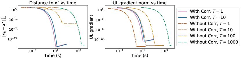
Figure 3: (left) Evolution of the distance of the UL iterate $x_{k}$ to the equilibrium $x^{\star}$ vs time (in seconds). (right) evolution of the norm of approximate gradient $d_{k}$ vs time in seconds. In all cases, algorithms are run until convergence, i.e. ${\left\lVert d_{k}\right\rVert}$ converges to $0$.

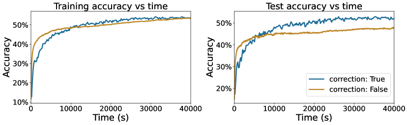
Figure 4: Evolution in time of the training and test accuracy of a ResNet18 model on Cifar10 dataset. Each iteration corresponds to the accuracy of the model with parameter $y_{k}$ trained on a synthetic dataset of $100$ points $x_{k}$ to minimize the LL objective. The synthetic points $x_{k}$ are learned by minimizing the training error when using the running model $y_{k}$.

E.2 Dataset Distillation on Cifar10

We consider the task of learning a small synthetic dataset so that a classifier trained on such a dataset achieves a small error on a training set. More formally, we consider a classification problem with $C$ classes using a model with parameters $y$ and a training dataset $\mathcal{D}_{tr}=\{(\xi_{i},c_{i})\}$ consisting of $N$ i.i.d. samples $\xi_{i}$ and corresponding labels $c_{i}$. The goal is to learn a synthetic dataset of $FC$ points, where $F$ is a positive integer, such that each class $c$ contains $F$ representative samples. We can collect the synthetic points into a vector $x$ to be learned and denote by $\mathcal{D}_{x}$ the synthetic dataset. For a given dataset $\mathcal{D}$, denote by $\mathcal{L}_{\mathcal{D}}(y)$ the cross-entropy loss of a model with parameters $y$ evaluated on $\mathcal{D}$. The bi-level formulation of the distillation task consists in optimizing a lower-level objective $g(x,y)=\mathcal{L}_{\mathcal{D}_{x}}(y)$ to learn the model parameters $y$ that best predicts the classes of the synthetic dataset. The upper-level objective $g(x,y)=\mathcal{L}_{\mathcal{D}_{tr}}(y)$ evaluates the optimal model on the training set and optimizes the synthetic samples.

Setup

. We consider a setup similar to [52] for distilling Cifar10 [27] on $100$ synthetic points. We set $F{=}10$, thus requiring $10$ synthetic points for each of the $C{=}10$ classes of Cifar10. We then use ResNet18 [22] as a classifier and apply Algorithm 1 to learn the optimal synthetic points. For the lower level, we use gradient descent with $1$ unrolled iteration (i.e. $T=1$, $M=0$) and a step-size of $\alpha{=}0.001$. For the upper level, we use Adam optimizer [26], with the default parameters, a step-size of $\gamma=0.01$ and a batch-size of $1024$. When using the corrective term, we use the update equation Equation 154 with a step-size $\beta=0.0001$.

Results.

Figure 4 shows the evolution of the training and test accuracy of the model as a function of time in two settings, either with or without correction. While the training accuracy for both versions of the algorithm is similar, the corrective term yields an improved final test accuracy ($54.19\%$ vs $48.6\%$). Note that these accuracies are of the same order as those obtained in [51] suggesting that distilling Cifar10 in only $100$ samples is not sufficient to capture all variability in the dataset. While the additional correction increases the computational cost per iteration, it provides a better gradient estimate which results in a faster/better performance overall.

References

• Ablin et al. [2020] Pierre Ablin, Gabriel Peyré, and Thomas Moreau. Super-efficiency of automatic differentiation for functions defined as a minimum. In International Conference on Machine Learning, pages 32–41. PMLR, 2020.
• Arbel and Mairal [2021] Michael Arbel and Julien Mairal. Amortized implicit differentiation for stochastic bilevel optimization. working paper or preprint, November 2021. URL https://hal.archives-ouvertes.fr/hal-03455458.
• Attouch et al. [2013] Hedy Attouch, Jérôme Bolte, and Benar Fux Svaiter. Convergence of descent methods for semi-algebraic and tame problems: proximal algorithms, forward–backward splitting, and regularized gauss–seidel methods. Mathematical Programming, 137(1):91–129, 2013.
• Austin and Braam [1995] David M Austin and Peter J Braam. Morse-bott theory and equivariant cohomology. In The Floer memorial volume, pages 123–183. Springer, 1995.
• Baydin et al. [2018] Atilim Gunes Baydin, Barak A Pearlmutter, Alexey Andreyevich Radul, and Jeffrey Mark Siskind. Automatic differentiation in machine learning: a survey. Journal of machine learning research, 18, 2018.
• Bertinetto et al. [2018] Luca Bertinetto, Joao F Henriques, Philip HS Torr, and Andrea Vedaldi. Meta-learning with differentiable closed-form solvers. arXiv preprint arXiv:1805.08136, 2018.
• Blondel et al. [2021] Mathieu Blondel, Quentin Berthet, Marco Cuturi, Roy Frostig, Stephan Hoyer, Felipe Llinares-López, Fabian Pedregosa, and Jean-Philippe Vert. Efficient and modular implicit differentiation. arXiv preprint arXiv:2105.15183, 2021.
• Bolte et al. [2021] Jérôme Bolte, Tam Le, Edouard Pauwels, and Tony Silveti-Falls. Nonsmooth implicit differentiation for machine-learning and optimization. Advances in neural information processing systems, 34:13537–13549, 2021.
• Bolte et al. [2022a] Jérôme Bolte, Ryan Boustany, Edouard Pauwels, and Béatrice Pesquet-Popescu. Nonsmooth automatic differentiation: a cheap gradient principle and other complexity results. arXiv preprint arXiv:2206.01730, 2022a.
• Bolte et al. [2022b] Jérôme Bolte, Edouard Pauwels, and Samuel Vaiter. Automatic differentiation of nonsmooth iterative algorithms. arXiv preprint arXiv:2206.00457, 2022b.
• Cohen [1991] Ralph L Cohen. Topics in Morse theory. Stanford University Department of Mathematics, 1991.
• Daneri and Savaré [2010] Sara Daneri and Giuseppe Savaré. Lecture notes on gradient flows and optimal transport. arXiv preprint arXiv:1009.3737, 2010.
• Dempe et al. [2007] S Dempe, J Dutta, and BS Mordukhovich. New necessary optimality conditions in optimistic bilevel programming. Optimization, 56(5-6):577–604, 2007.
• Domke [2012] Justin Domke. Generic methods for optimization-based modeling. In Artificial Intelligence and Statistics, pages 318–326. PMLR, 2012.
• Draxler et al. [2018] Felix Draxler, Kambis Veschgini, Manfred Salmhofer, and Fred Hamprecht. Essentially no barriers in neural network energy landscape. In International conference on machine learning, pages 1309–1318. PMLR, 2018.
• Feehan [2020] Paul Feehan. On the morse–bott property of analytic functions on banach spaces with łojasiewicz exponent one half. Calculus of Variations and Partial Differential Equations, 59(2):1–50, 2020.
• Feurer and Hutter [2019] Matthias Feurer and Frank Hutter. Hyperparameter optimization. In Automated machine learning, pages 3–33. Springer, Cham, 2019.
• Franceschi et al. [2018] Luca Franceschi, Paolo Frasconi, Saverio Salzo, Riccardo Grazzi, and Massimiliano Pontil. Bilevel programming for hyperparameter optimization and meta-learning. In International Conference on Machine Learning, pages 1568–1577. PMLR, 2018.
• Ghadimi and Wang [2018] Saeed Ghadimi and Mengdi Wang. Approximation methods for bilevel programming. arXiv preprint arXiv:1802.02246, 2018.
• Gould et al. [2016] Stephen Gould, Basura Fernando, Anoop Cherian, Peter Anderson, Rodrigo Santa Cruz, and Edison Guo. On differentiating parameterized argmin and argmax problems with application to bi-level optimization. arXiv preprint arXiv:1607.05447, 2016.
• Guo et al. [2015] Lei Guo, Gui-Hua Lin, and Jane J Ye. Solving mathematical programs with equilibrium constraints. Journal of Optimization Theory and Applications, 166(1):234–256, 2015.
• He et al. [2015] Kaiming He, Xiangyu Zhang, Shaoqing Ren, and Jian Sun. Deep Residual Learning for Image Recognition. 2016 IEEE Conference on Computer Vision and Pattern Recognition (CVPR), pages 770–778, 2015. doi: 10.1109/CVPR.2016.90.
• Hong et al. [2020] Mingyi Hong, Hoi-To Wai, Zhaoran Wang, and Zhuoran Yang. A two-timescale framework for bilevel optimization: Complexity analysis and application to actor-critic. arXiv preprint arXiv:2007.05170, 2020.
• Ji and Liang [2021] Kaiyi Ji and Yingbin Liang. Lower bounds and accelerated algorithms for bilevel optimization. arXiv preprint arXiv:2102.03926, 2021.
• Ji et al. [2021] Kaiyi Ji, Junjie Yang, and Yingbin Liang. Bilevel optimization: Convergence analysis and enhanced design. In International Conference on Machine Learning, pages 4882–4892. PMLR, 2021.
• Kingma and Ba [2015] Diederik P. Kingma and Jimmy Ba. Adam: A method for stochastic optimization. In Yoshua Bengio and Yann LeCun, editors, 3rd International Conference on Learning Representations, ICLR 2015, San Diego, CA, USA, May 7-9, 2015, Conference Track Proceedings, 2015.
• Krizhevsky et al. [2009] Alex Krizhevsky, Geoffrey Hinton, et al. Learning multiple layers of features from tiny images. 2009.
• Lang [2012] Serge Lang. Fundamentals of differential geometry, volume 191. Springer Science & Business Media, 2012.
• Lee [2003] John M. Lee. Introduction to Smooth Manifolds. Springer Science & Business Media, 2003. ISBN 978-0-387-95448-6. Google-Books-ID: eqfgZtjQceYC.
• Li et al. [2018] Hao Li, Zheng Xu, Gavin Taylor, Christoph Studer, and Tom Goldstein. Visualizing the loss landscape of neural nets. Advances in neural information processing systems, 31, 2018.
• Li et al. [2019] Zhuchun Li, Yi Liu, and Xiaoping Xue. Convergence and stability of generalized gradient systems by łojasiewicz inequality with application in continuum kuramoto model. Discrete & Continuous Dynamical Systems, 39(1):345, 2019.
• Liao et al. [2018] Renjie Liao, Yuwen Xiong, Ethan Fetaya, Lisa Zhang, KiJung Yoon, Xaq Pitkow, Raquel Urtasun, and Richard Zemel. Reviving and improving recurrent back-propagation. In International Conference on Machine Learning, pages 3082–3091. PMLR, 2018.
• Liu et al. [2021a] Risheng Liu, Jiaxin Gao, Jin Zhang, Deyu Meng, and Zhouchen Lin. Investigating bi-level optimization for learning and vision from a unified perspective: A survey and beyond. arXiv preprint arXiv:2101.11517, 2021a.
• Liu et al. [2021b] Risheng Liu, Xuan Liu, Shangzhi Zeng, Jin Zhang, and Yixuan Zhang. Value-function-based sequential minimization for bi-level optimization. arXiv preprint arXiv:2110.04974, 2021b.
• Liu et al. [2021c] Risheng Liu, Yaohua Liu, Shangzhi Zeng, and Jin Zhang. Towards gradient-based bilevel optimization with non-convex followers and beyond. Advances in Neural Information Processing Systems, 34, 2021c.
• Lojasiewicz [1982] Stanislaw Lojasiewicz. Sur les trajectoires du gradient d’une fonction analytique. Seminari di geometria, 1983:115–117, 1982.
• Lorraine et al. [2020] Jonathan Lorraine, Paul Vicol, and David Duvenaud. Optimizing millions of hyperparameters by implicit differentiation. In International Conference on Artificial Intelligence and Statistics, pages 1540–1552. PMLR, 2020.
• Mairal et al. [2011] Julien Mairal, Francis Bach, and Jean Ponce. Task-driven dictionary learning. IEEE transactions on pattern analysis and machine intelligence, 34(4):791–804, 2011.
• Martınez-Alfaro et al. [2016] J Martınez-Alfaro, IS Meza-Sarmiento, and R Oliveira. Topological classification of simple morse bott functions on surfaces. Real and complex singularities, 675:165–179, 2016.
• Merlet and Nguyen [2013] Benoît Merlet and Thanh Nhan Nguyen. Convergence to equilibrium for discretizations of gradient-like flows on riemannian manifolds. Differential and Integral Equations, 26(5/6):571–602, 2013.
• Panageas and Piliouras [2016] Ioannis Panageas and Georgios Piliouras. Gradient descent only converges to minimizers: Non-isolated critical points and invariant regions. arXiv preprint arXiv:1605.00405, 2016.
• Pedregosa [2016] Fabian Pedregosa. Hyperparameter optimization with approximate gradient. In International conference on machine learning, pages 737–746. PMLR, 2016.
• Rajeswaran et al. [2019] Aravind Rajeswaran, Chelsea Finn, Sham M Kakade, and Sergey Levine. Meta-Learning with Implicit Gradients. In H. Wallach, H. Larochelle, A. Beygelzimer, F. d\textquotesingle Alché-Buc, E. Fox, and R. Garnett, editors, Advances in Neural Information Processing Systems 32 (NeurIPS). Curran Associates, Inc., 2019.
• Rezende and Mohamed [2015] Danilo Rezende and Shakir Mohamed. Variational inference with normalizing flows. In International conference on machine learning, pages 1530–1538. PMLR, 2015.
• Robinson [2012] Rex Clark Robinson. An introduction to dynamical systems: continuous and discrete, volume 19. American Mathematical Soc., 2012.
• Rudin et al. [1976] Walter Rudin et al. Principles of mathematical analysis, volume 3. McGraw-hill New York, 1976.
• Shaban et al. [2019] Amirreza Shaban, Ching-An Cheng, Nathan Hatch, and Byron Boots. Truncated back-propagation for bilevel optimization. In The 22nd International Conference on Artificial Intelligence and Statistics, pages 1723–1732. PMLR, 2019.
• Singh et al. [2019] Rahul Singh, Maneesh Sahani, and Arthur Gretton. Kernel Instrumental Variable Regression. arXiv:1906.00232 [cs, econ, math, stat], June 2019. URL http://arxiv.org/abs/1906.00232. arXiv: 1906.00232.
• Stackelberg [1934] H.F. Von Stackelberg. MarktformundGleichgewicht. Springer, 1934.
• Vicol et al. [2021] Paul Vicol, Jonathan Lorraine, David Duvenaud, and Roger Grosse. Implicit regularization in overparameterized bilevel optimization. In ICML 2021 Beyond First Order Methods Workshop, 2021.
• Wang et al. [2018a] Tongzhou Wang, Jun-Yan Zhu, Antonio Torralba, and Alexei A Efros. Dataset distillation. arXiv preprint arXiv:1811.10959, 2018a.
• Wang et al. [2018b] Wei Wang, Yuan Sun, and Saman Halgamuge. Improving mmd-gan training with repulsive loss function. arXiv preprint arXiv:1812.09916, 2018b.
• Wiesemann et al. [2013] Wolfram Wiesemann, Angelos Tsoukalas, Polyxeni-Margarita Kleniati, and Berç Rustem. Pessimistic bilevel optimization. SIAM Journal on Optimization, 23(1):353–380, 2013.
• Xu and Ye [2014] Mengwei Xu and Jane J Ye. A smoothing augmented lagrangian method for solving simple bilevel programs. Computational Optimization and Applications, 59(1):353–377, 2014.
• Ye and Ye [1997] JJ Ye and XY Ye. Necessary optimality conditions for optimization problems with variational inequality constraints. Mathematics of Operations Research, 22(4):977–997, 1997.
• Ye and Zhu [1995] JJ Ye and DL Zhu. Optimality conditions for bilevel programming problems. Optimization, 33(1):9–27, 1995.
• Ye et al. [1997] JJ Ye, DL Zhu, and Qiji Jim Zhu. Exact penalization and necessary optimality conditions for generalized bilevel programming problems. SIAM Journal on optimization, 7(2):481–507, 1997.
• Zemkoho [2016] Alain B Zemkoho. Solving ill-posed bilevel programs. Set-Valued and Variational Analysis, 24(3):423–448, 2016.