Statistical Equilibrium of Large Scales in three-dimensional Hydrodynamic Turbulence

Abstract

We investigate experimentally three-dimensional (3D) hydrodynamic turbulence at scales larger than the forcing scale. We manage to perform a scale separation between the forcing scale and the container size by injecting energy into the fluid using centimetric magnetic particles. We measure the statistics of the fluid velocity field at scales larger than the forcing scale (energy spectra, velocity distributions, and energy flux spectrum). In particular, we show that the large-scale dynamics are in statistical equilibrium and can be described with an effective temperature, although not isolated from the turbulent Kolmogorov cascade. In the large-scale domain, the energy flux is zero on average but exhibits intense temporal fluctuations. Our work paves the way to use equilibrium statistical mechanics to describe the large-scale properties of 3D turbulent flows.

Introduction.—

Three-dimensional (3D) hydrodynamics turbulence has been extensively studied to characterize the energy transfers in the inertial range, the interval between the energy injection scale and the small (dissipative) scale Richardson ; Kolmogorov41 ; K41b ; Frisch ; Pope . While they control many properties of 3D turbulent flows, e.g., mixing in industrial flows, or transport of tracers in geophysical and astrophysical turbulent flows Moffatt , the large-scale properties of turbulence, the scales larger than the forcing scale, have been less investigated. Indeed, in most experiments and direct numerical simulations (DNS), 3D turbulent flows are forced at a scale comparable to the container size to study the turbulent energy cascade within the inertial range. However, it has been conjectured that the large-scale modes of turbulent flows possess the same energy and are in a statistical stationary equilibrium regime Burgers29 ; Frisch ; Hopf ; Lee ; Kraichnan . This equipartition regime, also called thermal equilibrium, would occur if no mean energy flux is transferred from the forcing scale to the large scales. Such a statistical equilibrium is difficult to observe in most experimental systems and numerical simulations because there is no scale separation between the forcing scale and the container size. Numerical simulations have recently confirmed the statistical equilibrium in 3D forced turbulent flows for the spectrally truncated Navier-Stokes equations AlexakisJFM2020 and the truncated Euler equation Cichowlas2005 ; Dallas2015 ; AlexakisJFM2019 ; Verma2020 , but experimental evidence of this regime remains elusive.

Here, we generate 3D hydrodynamic turbulence using centimetric magnetic particles immersed in a large fluid reservoir. This method provides a wide interval between the energy injection scale and the container size. We observe a statistical equilibrium regime in this large-scale interval while a turbulent cascade develops in the inertial range. We also show that the effective temperature of the statistical equilibrium regime is related to the injection of energy. Note that large-scale structures in decaying 3D turbulence have been investigated Batchelor56 ; Saffman67 ; Davidson ; Lesieur ; DavidsonJFM2012 ; YoshimatsuPRF2019 , but are different from the stationary (forcing) case AlexakisJFM2019 . Other turbulent systems also exhibit large-scale statistical equilibrium, e.g., in wave turbulence with no inverse cascade, such as capillary waves Balkovsky1995 ; Michel2017 ; Abdurakhimov2015 , bending waves in mechanical plates MiquelPRE2021 , or optical waves Josserand05 . Conversely, the presence of an inverse cascade implies that two-dimensional hydrodynamic turbulence Kraichnan67 , gravity wave turbulence FalconPRL2020 , or acoustic wave turbulence in superfluid Ganshin2008 do not exhibit a statistical equilibrium regime.

Theoretical backgrounds.—

In the case of nonhelical, incompressible, inviscid, and force-free turbulent flows, Kraichnan Kraichnan derived the statistical equilibrium energy spectrum $E_{T}(k)$ for low wavenumbers $k$

$$E_{T}(k)=\frac{4\pi\alpha k^{2}}{\alpha^{2}-\beta^{2}k^{2}}.$$ (1)

$\alpha$, $\beta$ are determined by the total energy and the helicity of the system. This result referred to as absolute equilibrium, is related to classical equilibrium statistical mechanics and is equivalent to the equipartition of the total kinetic energy among the large-scale Fourier modes Rose1978 ; Lesieur ; Hopf ; Lee . One can also say that the large-scale equipartition implies that the spectral energy density per unit mass $E_{T}(k)\mathrm{d}k$ is equal to the number of modes times the energy per mode per mass, i.e.,

$$E_{T}(k)\mathrm{d}k=\frac{4\pi k_{\rm B}{T}}{\rho}k^{2}\mathrm{d}k$$ (2)

with $k_{\rm B}$ the Boltzmann constant, $\rho$ the fluid density, and $T$ a temperature in a classical thermodynamic equilibrium sense. Therefore, one obtains the expression which is equivalent to Eq. (1) when $\beta k\ll\alpha$. Note that deviations from Eq. (1) are expected for a broadband spectral forcing instead of a narrow one AlexakisJFM2019 or in the case of anisotropic turbulence Thalabard2015 .

By assuming high-Reynolds number isotropic turbulence, the energy spectrum in the inertial range (i.e., for high $k$) is given by the Kolmogorov spectrum Kolmogorov41

$$E_{K}(k)=C_{K}\epsilon^{2/3}k^{–5/3}$$ (3)

with $C_{K}\simeq 1.6$ the experimentally measured Kolmogorov constant SaddoughiJFM94 , and $\epsilon$ the rate of energy dissipation per unit mass. In the stationary regime, $\epsilon$ is constant and equal to the energy flux transferred from the forcing scale to the dissipation scale. Therefore, $\epsilon$ is also equal to the energy injection rate in the stationary regime.

Experimental setup.—

We inject energy homogeneously into the fluid using small magnetic particles. The nonlinear transfer of energy and turbulent cascade towards small scales (inertial range) have been characterized using this method CazaubielPRF2021 . To measure the large-scale properties of turbulence, we scaled up this experimental system. A plexiglass square container of length $L=32$ cm and height $h=22$ cm is filled with water (22.5 L) and sealed by a transparent lid. This fluid container sits between a pair of Helmholtz coils (0.49 m inner diameter and 1 m outer diameter). The pair of coils is powered by a sinusoidal current (Itech IT7815 AC 15 kW power supply) and generates a vertical oscillating magnetic field $B(t)$ with an amplitude $B\in[0,360]$ G and a frequency $F\in[0,25]$ Hz. This AC magnetic field is homogeneous within all the volume of the fluid container (5% accuracy) and transfers kinetic energy to $N$ neodymium magnets encapsulated in plexiglass shells (1 cm), which are immersed in the fluid ($N\in[50,450]$). The volume fraction of the magnetic particles is smaller than 1.5%. The kinetic energy of the magnetic particles is then transferred to the surrounding fluid randomly in both space and time (see FalconEPL2013 ; FalconPRF2017 ; CazaubielPRF2021 and movies in the Supplemental Material SuppMat ; Note ). The forcing scale is estimated to be 5 cm. It corresponds to the integral scale $L_{i}$ defined as the abscissa of the maximum of the energy spectrum (see below). Note that $L_{i}$ cannot be accurately computed from the autocorrelation function of the velocity field since the container size $L$ is not eight times larger than the integral scale Pope ; CazaubielPRF2021 ; ONeill2004 . The fluid velocity is measured locally by nonintrusive Laser Doppler Velocimetry (LDV Dantec Flow Explorer 1D) with a sampling frequency of 250 Hz. We perform Particle Image Velocimetry (PIV) Thielicke2014 to measure the fluid velocity field in a horizontal $xy$ plane ($32\times 32$ cm²). The fluid is seeded with Polyamide fluid tracers ($50\text{\,}\upmu\mathrm{m}$) illuminated by a horizontal laser sheet and a high-speed camera (Phantom V1840, 2048​ $\times$​ 1952 pixels² at 200 fps), located on the top of the fluid container, records time series of images. The mean fluid velocity is smaller than the standard deviation of the velocity fluctuations $\sigma_{u}$ ($<10$%), such that one can assume that there is no mean flow. The isotropy of the velocity field is also checked for different values of $N$ Note2 . Typical values of the turbulent flow are the following: the dissipation rate $\epsilon$ is $3\times 10^{-4}$ m²/s³, the Reynolds number at the integral scale $L_{i}\simeq 5$ cm is 650, and the Reynolds number at the Taylor scale $L_{\lambda}\simeq 7.6$ mm is ${\rm Re}_{\lambda}=100$. We have ${\rm Re}_{\lambda}\in[56,100]$ when changing the experimental parameters ($F$, $N$, or $B$).

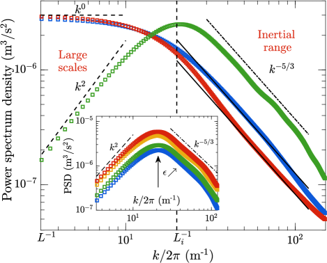
Figure 1: 3D power spectrum density $E(k)$ (green) derived from the 1D spectrum of the longitudinal velocity $E_{uu}(k_{x})$ (red), and transverse velocity $E_{vv}(k_{x})$ (blue), (Eq. (4)). Dashed line: $k^{2}$ power law illustrating the large-scale statistical equilibrium regime. Dot-dashed line: $k^{-5/3}$ power law illustrating the inertial range of the turbulent cascade. The vertical dashed line corresponds to the inverse of the integral scale $k_{i}/2\pi=1/L_{i}$ and separates the large-scale domain ($k<k_{i}$) from the inertial range ($k>k_{i}$). The PIV measurements are performed at $F=20$ Hz, $B=290$ G and $N=55$. Inset: Power spectrum densities at different $\epsilon\in[1.1,3.2]\times 10^{-4}$ m²/s³.

Spatial power spectrum.—

The longitudinal and transverse horizontal fluid velocities are defined as $u(x,t)$ and $v(x,t)$. We first measure the longitudinal $E_{uu}(k_{x})$ and transverse $E_{vv}(k_{x})$ spectra (Fig. 1). The inertial range is consistent with the Kolmogorov prediction over a decade. The power spectra are proportional to $k_{x}^{-5/3}$ in the inertial range and the ratio between the unidimensional (1D) power spectra is equal to $E_{vv}(k_{x})/E_{uu}(k_{x})=4/3$ Pope (black lines in Fig. 1). In the case of isotropic turbulence, the 3D power spectrum $E(k)$ is derived from the longitudinal and transverse spectra Pope ; Davidson

$$E(k)=-k\frac{\mathrm{d}}{\mathrm{d}k}\left[\frac{1}{2}E_{uu}(k_{x})+E_{vv}(k_{x})\right]\,{\rm.}$$ (4)

The energy spectrum $E(k)$ is shown in Fig. 1. A $k^{2}$ power law is observed in the energy spectra at lower wavenumbers, illustrating the statistical equilibrium regime, while a $k^{-5/3}$ power law is observed at higher wavenumbers, indicating a direct energy cascade in the inertial range. In between these regimes, the wavenumbers close to the value $k_{i}=2\pi/L_{i}$ suggest that the statistical equilibrium state and the out-of-equilibrium one interact with each other (see below).

Effective temperature.—

Both $k^{2}$ and $k^{-5/3}$ power laws are consistently observed in the energy spectra when increasing the energy injection rate $\epsilon$ (inset of Fig. 1). For each 3D spectrum $E(k$), we compute the effective temperature by integrating both members of Eq. (2) in the large-scale interval $k\in[k_{L}=2\pi/L$, $k_{i}=2\pi/L_{i}]$

$$T_{exp}=\frac{3\rho}{32\pi^{4}k_{\rm B}}\frac{L^{3}L_{i}^{3}}{L^{3}-L_{i}^{3}}\int_{k_{L}}^{k_{i}}E(k)\mathrm{d}k\,{\rm.}$$ (5)

$T_{exp}$ is shown in Fig. 2 as a function of the energy injection rate $\epsilon$ ($\times$). One can also estimate the temperature by fitting directly the experimental 3D spectra with Eq. (2), which leads to similar values of the temperature ($\circ$ in Fig. 2). $T_{exp}$ is found to be 13 orders of magnitude higher than the room temperature and proportional to $\epsilon^{2/3}$ (Fig. 2). This result is explained by equating Eqs. (2) and (3), which gives the relationship

$$T=\frac{\rho C_{K}}{4\pi k_{\rm B}}k_{i}^{-11/3}\epsilon^{2/3}.$$ (6)

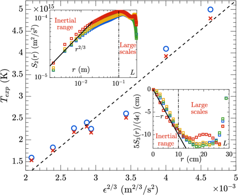
Figure 2: Effective temperature $T_{exp}$ of the statistical equilibrium regime of the large scales for different energy injection rates $\epsilon$. The energy injection rate $\epsilon$ is measured using $\epsilon=2\nu\int_{2\pi/L}^{\infty}k^{2}E(k)dk$. $T_{exp}$ is measured from the 3D spectra shown in Fig. 1 using Eqs. (2) ($\circ$) and (5) ($\times$). The solid dashed line corresponds to Eq. (6) using $k_{i}/2\pi=13.3$ m^-1. Insets: Structure functions $S_{2}(r)$ (top) and $S_{3}(r)/(4\epsilon/5)$ (bottom) for different $\epsilon$ (same colors as in the inset of Fig. 1). Solid lines correspond to $r^{2/3}$ and $-r$, respectively.

Structure functions.—

The velocity increments at a distance $r$, $\mathcal{S}_{i}(r)=\langle[v(x+r)-v(x)]^{i}\rangle$ are now computed from the PIV measurements. The insets of Fig. 2 show that $\mathcal{S}_{2}(r)\sim(\epsilon r)^{2/3}$ and $\mathcal{S}_{3}(r)=-4\epsilon r/5$ in the inertial range, as predicted theoretically Kolmogorov41 ; K41b ; Pope . For large scales (i.e., $r>0.1$ m), $\mathcal{S}_{2}(r)$ and $\mathcal{S}_{3}(r)$ are found to be roughly independent of $r$, except when $r\simeq L$. We also found that $\mathcal{S}_{2}(r)\simeq 2\sigma_{u}^{2}$, suggesting that the velocities are uncorrelated at long distances, as expected Davidson .

Velocity probability distribution.—

The probability distribution functions (PDF) of the velocity field (Fig. 3) are found to be strongly non-Gaussian probably because the PDFs of the Lagrangian magnetic particle velocity are stretched exponentials (see Supp. Mat. SuppMat ). However, we show that the large-scale modes are normally distributed by applying a spatial low-pass filter to the velocity field, confirming that the large-scale modes have reached a statistical equilibrium. The Kurtosis of the low-pass filtered velocity distribution is equal to 3 (inset Fig. 3). The shape of the PDF of the low-pass filtered velocities is also independent of the energy injection rate $\epsilon$, which is illustrated by the constant value of the kurtosis (inset Fig. 3). High-pass filtering of the velocity field also shows that the non-Gaussianity of the PDFs is reminiscent of the magnetic particle velocity one.

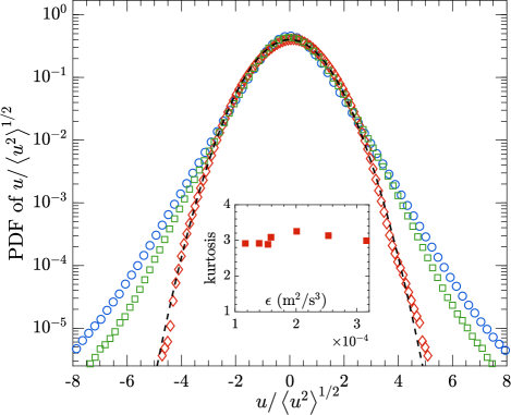
Figure 3: Probability density functions (PDF) of the normalized fluid velocity fluctuations $u/\sqrt{\langle u^{2}\rangle}$ of ($\Diamond$) large-scale modes, ($\square$) all modes, and ($\circ$) small-scale modes for $\sigma_{u}=0.6$ cm/s. The cutoff value of the filter is equal to $k/2\pi=9.4$ (m^-1). The black dashed line represents a Gaussian distribution. Inset: Kurtosis ($K=\langle u^{4}\rangle/\langle u^{2}\rangle^{2}$) of the large-scale modes as a function of $\epsilon$ ($\sigma_{u}\in[0.6,1.3]$ cm/s).

Mean energy flux.—

Measuring the energy flux is essential to understanding the dynamics of turbulent phenomena Verma . We compute the time-averaged energy flux spectrum $\overline{\Pi}(k)$ from the expression $\Pi(k,t)=\langle\mathbf{v}^{<}_{k}\cdot[\mathbf{v}^{<}_{k}\cdot\nabla\mathbf{v}^{>}_{k}]\rangle_{r}+\langle\mathbf{v}^{<}_{k}\cdot[\mathbf{v}^{>}_{k}\cdot\nabla\mathbf{v}^{>}_{k}]\rangle_{r}$ Frisch , where $\mathbf{v}^{<}_{k}(\mathbf{r})\equiv\int_{0}^{k}\mathbf{\widehat{v}}(k^{\prime})e^{i\mathbf{k^{\prime}\cdot r}}\mathrm{d}k^{\prime}$ is the low-filtered velocity field at the wavenumber $k$, $\mathbf{v}^{>}_{k}(\mathbf{r})\equiv\int_{k}^{\infty}\widehat{\mathbf{v}}(k^{\prime})e^{i\mathbf{k^{\prime}\cdot r}}\mathrm{d}k^{\prime}$ the high-filtered one, and $\mathbf{\widehat{v}}$ is the Fourier transform of the velocity field $\mathbf{v}$. The zero-mean energy flux measured at low wavenumbers confirms the statistical equilibrium regime (Fig. 4). The interval in which the mean energy flux is zero corresponds to the same interval in which the $k^{2}$ power law of the energy spectrum is observed. In the inertial range, the energy flux is positive and implies a direct energy cascade towards high wavenumbers, corresponding to the turbulent cascade shown in Fig. 1. For wavenumbers $k/2\pi$ higher than 100 m^-1, the energy flux strongly decreases, which is consistent with Fig. 1.

Energy flux fluctuations.—

Although no energy cascades within the large scales in equipartition, intense temporal fluctuations of the energy flux $\Pi(k,t)$ are observed (bottom inset of Fig. 4 - see also Supp. Mat. SuppMat ). This highlights that the large-scale domain is not isolated from the inertial range. Within the large-scale interval, the energy flux follows a Gaussian distribution (bottom inset of Fig. 4), whose standard deviation $\sigma_{\Pi}(k)=\left[\overline{\Pi(k,t)^{2}}\right]^{1/2}$ is proportional to $k^{2}$ (top inset), similarly to the energy spectrum $E(k)$. We can thus infer that $\sigma_{\Pi}(k)/E(k)\sim k^{0}$ for $k<k_{i}$. The damped fluctuations of zero-mean energy flux observed at low wavenumbers (top inset Fig. 4) have also been reported in DNS Dallas2015 ; AlexakisJFM2020 . The top inset of Fig. 4 also shows that these fluctuations are intense within the direct cascade but are strongly damped by viscous dissipation at high wavenumbers.

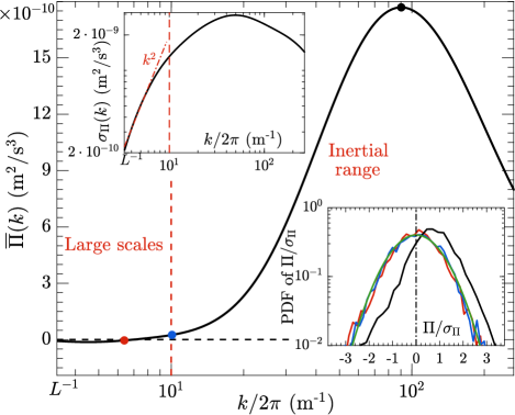
Figure 4: Time-averaged energy flux spectrum $\overline{\Pi}(k)$. At large scales ($k<k_{i}$), zero-mean energy flux is measured (equipartition). In the inertial range ($k>k_{i}$), the energy flux is positive and implies a direct cascade of energy. Insets: (top) Standard deviation of the energy flux spectrum $\sigma_{\Pi}(k)$. (bottom): PDFs of the fluctuations of the energy flux $\Pi/\sigma_{\Pi}$ for three values of the wavenumber $k$ (colored bullets). The green line represents a Gaussian distribution.

Temporal power spectrum.—

We now measure the temporal spectrum $E_{u}(f)$ of the horizontal velocity $u(t)$ (Fig. 5). The signal is recorded for $\mathcal{T}=5$  hours to converge the statistics at low frequencies ($f<f_{i}$), which represent the large-scale modes. To avoid a significant increase in the fluid temperature, we repeatedly performed LDV measurements for 100 s and then we let the fluid cool down for 10 min. The signal $u(t)$ is shown in the inset of Fig. 5, with a low-pass filtered signal (black) to emphasize the slow modes of the temporal signal. The frequency spectrum shown in Fig. 5 is proportional to $f^{-5/3}$ at high frequencies ($f>f_{i}$). This is consistent with the $k^{-5/3}$ power law observed in the unidimensional energy spectrum, which implies a direct energy cascade in the inertial range (Fig. 1). This power law was predicted by the Tennekes’ model (large-scale advection of turbulent eddies) in isotropic turbulence without mean flow Tennekes ; CazaubielPRF2021 . At low frequencies ($f<f_{i}$), the frequency spectrum is found to be almost flat $f^{0}$, implying that large scales are uncorrelated. This is similar to the unidimensional spatial spectrum $E_{uu}(k)\sim k^{0}$ at large scales (Fig. 1), suggesting that we observe the statistical equilibrium regime at low frequencies.

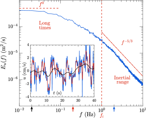
Figure 5: Temporal power spectrum density of the horizontal velocity $E_{u}(f)$. The dashed line represents a $f^{0}$ power law and the dot-dashed line represents a $f^{-5/3}$ power law. The forcing parameters are identical to Fig. 1. $f_{i}$ indicates the beginning of the inertial range, i.e., the typical correlation frequency of the flow. Inset: Horizontal velocity $u(t)$ low-pass filtered at 2 Hz (blue), 0.2 Hz (red), and 0.02 Hz (black), as illustrated by the colored arrows in the main figure.

Conclusion.—

We have experimentally shown that the large-scale dynamics in forced dissipative 3D hydrodynamic turbulence are in agreement with the statistical equilibrium prediction. This system is a remarkable example in which the large scales are in statistical equilibrium, while smaller scales are in an out-of-equilibrium stationary regime. A direct consequence of this experimental validation is that simulations leading to a statistical equilibrium regime, such as those of the truncated Euler equation Dallas2015 , could provide a new tool to efficiently simulate the large-scale dynamics of 3D turbulent flows in various fields. Our findings also pave the way to possibly use concepts of equilibrium statistical mechanics (such as fluctuation-dissipation and fluctuation theorems) for large-scale turbulent flows. It can help better understand the interactions between the degrees of freedom at equilibrium (large scales) with out-of-equilibrium structures (small scales), which are essential when studying turbulent phenomena. In the future, we will explore the transient regimes of the equilibrium regime of large scales, called the thermalization processes, by measuring the growth and decay of turbulence Saffman67 ; DavidsonJFM2012 . More generally, better identifying the mechanisms governing large-scale properties of turbulent flows such as statistical equilibrium, condensation, or inverse cascade, is of primary interest in 3D turbulence Alexakis2018 ; Dallas2015 ; Xia2011 ; FalconPRF2017 , wave turbulence Michel2017 ; FalconPRL2020 ; MiquelPRE2021 , and climate modeling ShawARFM2013 .

- (1) L. F. Richardson Weather Prediction by Numerical Process (Cambridge University Press, Cambridge, United Kingdom, 1922).
- (2) A. N. Kolmogorov, The local structure of turbulence in incompressible viscous fluid for very large Reynolds numbers, Dokl. Akad. Nauk SSSR 30, 9 (1941); reproduced in Proc. R. Soc. Lond. A 434, 9 (1991).
- (3) A. N. Kolmogorov, Dissipation of energy in the locally isotropic turbulence, Dokl. Akad. Nauk SSSR 32, 16 (1941), reproduced in Proc. R. Soc. Lond. A 434, 15 (1991).
- (4) U. Frisch Turbulence: The Legacy of A. N. Kolmogorov (Cambridge University Press, Cambridge, United Kingdom, 1995), and references therein.
- (5) S. B. Pope Turbulent flows (Cambridge University Press, Cambridge, 4th Ed., 2006)
- (6) H. K. Moffatt Magnetic Field Generation in Electrically Conducting Fluids (Cambridge University Press, Cambridge, United Kingdom, 1978)
- (7) J. M. Burgers, On the application of statistical mechanics to the theory of turbulent fluid motion, Proc. Roy. Neth. Acad. Soc. 32, 414, 643, 818 (1929), reprinted in F. T. M. Nieuwstadt and J. A. Steketee Selected Papers of J. M. Burgers (Springer, Dordrecht, 1995)
- (8) E. Hopf, Statistical hydromechanics and functional calculus, J. Rational Mech. Anal. 1, 87 (1952).
- (9) T. D. Lee, On some statistical properties of hydrodynamical and magneto-hydrodynamical fields, Quart. Appl. Math. 10, 69 (1952).
- (10) R. H. Kraichnan, Helical turbulence and absolute equilibrium, J. Fluid Mech. 59, 745 (1973)
- (11) A. Alexakis and M.-É. Brachet, Energy fluxes in quasi-equilibrium flows, J. Fluid Mech. 884, A33 (2020).
- (12) C. Cichowlas, P. Bonaïti, F. Debbasch, and M.-É. Brachet, Effective dissipation and turbulence in spectrally truncated Euler flows, Phys. Rev. Lett. 95, 264502 (2005).
- (13) V. Dallas, S. Fauve, and A. Alexakis, Statistical Equilibria of Large Scales in dissipative Hydrodynamic Turbulence, Phys. Rev. Lett. 115, 204501 (2015)
- (14) A. Alexakis and M.-É. Brachet, On the thermal equilibrium state of large-scale flows, J. Fluid Mech. 872, 594 (2019).
- (15) M. K. Verma, S. Bhattacharya, and S. Chatterjee, Euler turbulence and thermodynamic equilibrium, ArXiv:202409053v1 (2020); M. K. Verma, Boltzmann equation and hydrodynamic equations: their equilibrium and non-equilibrium behaviour, Phil. Trans. R. Soc. A 378 20190470 (2020).
- (16) G. K. Batchelor and I. Proudman, The large-scale structure of homogeneous turbulence, Phil. Trans. Roy. Soc. A 248, 369 (1956).
- (17) P. G. Saffman, The large-scale structure of homogeneous turbulence, J. Fluid Mech. 27, 581 (1967).
- (18) P. A. Davidson Turbulence (Oxford University Press, New-York, 2nd. Ed., 2015)
- (19) M. Lesieur Turbulence in fluids (Martinus Nijhoff Publishers, Dordrecht, 1987) pp. 205 - 211
- (20) P. Krogstad and P. Davidson, Is grid turbulence Saffman turbulence? J. Fluid Mech. 642, 373 (2010); P. Davidson, N. Okamoto, and Y. Kaneda, On freely decaying, anisotropic, axisymmetric Saffman turbulence. J. Fluid Mech. 706, 150 (2012).
- (21) K. Yoshimatsu and Y. Kaneda, No return to reflection symmetry in freely decaying homogeneous turbulence, Phys. Rev. Fluids 4, 024611 (2019)
- (22) G. Michel, F. Pétrélis, and S. Fauve, Observation of Thermal Equilibrium in Capillary Wave Turbulence, Phys. Rev. Lett. 118, 144502 (2017).
- (23) E. Balkovsky, G. Falkovich, V. Lebedev, and I. Ya. Shapiro, Large-scale properties of wave turbulence, Phys. Rev. E 52, 4537 (1995).
- (24) L. V. Abdurakhimov, M. Arefin, G. V. Kolmakov, A. A. Levchenko, Yu. V. Lvov, and I. A. Remizov, Bidirectional energy cascade in surface capillary waves, Phys. Rev. E 91, 023021 (2015).
- (25) B. Miquel, A. Naert, and S. Aumaître, Low-frequency spectra of bending wave turbulence, Phys. Rev. E 103, L061001 (2021).
- (26) C. Connaughton, C. Josserand, A. Picozzi, Y. Pomeau, and S. Rica, Condensation of Classical Nonlinear Waves, Phys. Rev. Lett. 95, 263901 (2005); C. Sun, S. Jia, C. Barsi, S. Rica, A. Picozzi, and J. W. Fleischer, Observation of the kinetic condensation of classical waves, Nature Phys. 8, 470 (2012); K. Baudin, A. Fusaro, K. Krupa, J. Garnier, S. Rica, G. Millot, and A. Picozzi, Classical Rayleigh-Jeans Condensation of Light Waves: Observation and Thermodynamic Characterization, Phys. Rev. Lett. 125, 244101 (2020)
- (27) R. H. Kraichnan, Inertial Ranges in Two‐Dimensional Turbulence, Phys. Fluids 10, 1417 (1967); J. Sommeria, Experimental study of the two-dimensional inverse energy cascade in a square box, J. Fluid Mech. 170, 139 (1986); J. Paret and P. Tabeling, Experimental observation of the two-dimensional inverse energy cascade, Phys. Rev. Lett. 79, 4162 (1997); A. von Kameke, F. Huhn, G. Fernández-García, A. P. Muñuzuri, and V. Pérez-Muñuzuri, Double cascade turbulence and Richardson dispersion in a horizontal fluid flow induced by Faraday waves, Phys. Rev. Lett. 107, 074502 (2011); N. Francois, H. Xia, H. Punzmann, and M. Shats, Inverse energy cascade and emergence of large coherent vortices in turbulence driven by Faraday waves. Phys. Rev. Lett. 110, 194501 (2013).
- (28) E. Falcon, G. Michel, G. Prabhudesai, A. Cazaubiel, M. Berhanu, N. Mordant, S. Aumaître, and F. Bonnefoy, Saturation of the Inverse Cascade in Surface Gravity-Wave Turbulence, Phys. Rev. Lett. 125, 134501 (2020).
- (29) A. N. Ganshin, V. B. Efimov, G. V. Kolmakov, L. P. Mezhov-Deglin, and P. V. E. McClintock, Observation of an inverse energy cascade in developed acoustic turbulence in superfluid helium, Phys. Rev. Lett. 101, 065303 (2008).
- (30) H. A. Rose and P. L. Sulem, Fully developed turbulence and statistical mechanics, J. Phys. II (France) 39, 441 (1978).
- (31) S. Thalabard, B. Saint-Michel, E. Herbert, F. Daviaud, and B. Dubrulle, A statistical mechanics framework for the large-scale structure of turbulent von Kármán flows, New J. Phys. 17, 063006 (2015).
- (32) S. G. Saddoughi and S. V. Veeravalli, Local isotropy in turbulent boundary layers at high Reynolds number, J. Fluid Mech. 268, 333 (1994).
- (33) E. Falcon, J.-C. Bacri, C. Laroche, Equation of state of a granular gas homogeneously driven by particle rotations, Europhys. Lett. 103, 64004 (2013)
- (34) E. Falcon, J.-C. Bacri, and C. Laroche, Dissipated power within a turbulent flow forced homogeneously by magnetic particles, Phys. Rev. Fluids 2, 102601(R) (2017)
- (35) A. Cazaubiel, J.-B. Gorce, J.-C. Bacri, M. Berhanu, C. Laroche, and E. Falcon, Three-dimensional turbulence generated homogeneously by magnetic particles, Phys. Rev. Fluids 6, L112601 (2021)
- (36) See Supplemental Material at http://link.aps.org/… for movies and further data analyses, which includes additional Refs. Rouyer .
- (37) In movies of Ref. SuppMat , note, in particular, the motions of the magnetic particles are not synchronized with the vertical oscillating magnetic field.
- (38) P. L. O’Neill, D. Nicolaides, D. R. Honnery, and J. Soria, Autocorrelation functions and the determination of integral length with reference to experimental and numerical data, in Proc. 15th Australasian Fluid Mech. Conf., edited by M. Behnia, W. Lin, and G. D. McBain (University of Sydney, Australia, 2004), pp. 1–4.
- (39) W. Thielicke and E. Stamhuis, PIVlab–towards user-friendly, affordable and accurate digital particle image velocimetry in MATLAB, J. Open Res. Softw. 2, 1 (2014).
- (40) The measured isotropy ratios, and , are smaller than 7% regardless of , confirming the isotropy of the velocity field.
- (41) M. K. Verma, Variable energy flux in turbulence, J. Phys. A 55, 13002 (2021).
- (42) H. Tennekes, Eulerian and lagrangian time microscales in isotropic turbulence, J. Fluid Mech. 67, 561 (1975).
- (43) A. Alexakis and L. Biferale, Cascades and transitions in turbulent flows, Phys. Rep. 767, 1 (2018).
- (44) H. Xia, D. Byrne, G. Falkovich, and M. Shats, Upscale energy transfer in thick turbulent fluid layers, Nat. Phys. 7, 321 (2011)
- (45) R. A. Shaw, Particle-turbulence interactions in atmospheric clouds, Annu. Rev. Fluid Mech. 35, 183 (2003)
- (46) F. Rouyer and N. Menon, Velocity Fluctuations in a Homogeneous 2D Granular Gas in Steady State, Phys. Rev. Lett. 85, 3676 (2000), T. P. C. Van Noije and M. H. Ernst, Velocity distributions in homogeneous granular fluids: the free and the heated case, Granular Matter 1, 57 (1998).