Research Joint Ventures:
The Role of Financial Constraints

Abstract

This paper provides a novel theory of research joint ventures for financially constrained firms. When firms choose R&D portfolios, an RJV can help to coordinate research efforts, reducing investments in duplicate projects. This can free up resources, increase the variety of pursued projects and thereby increase the probability of discovering the innovation. RJVs improve innovation outcomes when market competition is weak or external financing conditions are bad. An RJV may increase the innovation probability and nevertheless lower total R&D costs. RJVs that increase innovation also increase consumer surplus and tend to be profitable, but innovation-reducing RJVs also exist. Finally, we compare RJVs to innovation-enhancing mergers.

JEL Codes:	L13, L24, O31
Keywords:	Innovation, Research Joint Ventures, Financial Constraints,
	Mergers, Intensity of Competition, Licensing

1 Introduction

Innovation often involves large R&D investments. A well-known example is the pharmaceutical industry where blockbuster drugs can require high upfront R&D expenses. Similarly, automobile producers have recently spent £341 billion within five years to become successful players in the electric vehicle industry. The necessary investments and the required technological skills are so large that even industry giants rarely attempt to take on the task on their own. In the last few years, major players have agreed on research joint ventures (RJVs). For instance, Daimler and Geely jointly develop battery-driven Smart cars. PSA and Opel hooked up with Saft, a subsidiary of Total, to develop batteries. Together with BP, Daimler and BMW develop charging stations. Renault, Nissan and Mitsubishi Motors agreed on investing $26 billion to develop common platforms for electric vehicles. Further up in the value chain, suppliers of essential inputs have also joined forces. Not only are the required R&D investments large, there is also significant uncertainty about which technology the vehicles of the future will rely on. Today, most electric vehicles are powered by lithium-ion batteries, but this technology has significant drawbacks and automotive companies are additionally investing in alternative approaches. For example, Volvo and Daimler are collaborating on fuel-cell driven cars, while Ford and BMW have jointly invested in a startup developing solid-state batteries. In all these partnerships, at least some of the firms are competing or planning to compete in the product market.

Though competition policy investigates RJVs in various ways, it typically treats them more leniently than other forms of horizontal cooperation. For instance, the European Union addresses RJVs either under its merger regulation or under Article 101 of the EU treaty, depending on whether it is a full-function joint venture or not. In the latter case, even if an RJV has been found to have anti-competitive object or actual or potential competition-restricting effects (Article 101(1)), it may still be justified on the basis of efficiency gains under certain conditions (Article 101(3)). The legal situation in the United States is similar, with the 1993 National Cooperative Research and Production Act specifying that horizontal cooperation in RJVs is not per se illegal, but is to be evaluated under the “rule of reason”.

An important prerequisite to justify a friendly approach of competition policy towards RJVs is that they have beneficial effects on R&D activities. Existing literature focuses on knowledge spillovers as the main justification for RJVs. Our paper analyzes a different channel through which RJVs can lead to more innovation: When R&D costs are high (so that firms are financially constrained) and there is significant uncertainty about the right way to generate the desired innovative outcome, an RJV can help reduce investments in duplicate R&D projects, thereby freeing up funds that can be invested in previously unexplored approaches. To clarify conditions under which this is indeed the case, we introduce a model that combines financial constraints and uncertainty about the right way to generate the desired innovation. Contrary to previous theoretical literature on RJVs, the firms not only choose how much to invest in, but also how to spread investments over different R&D projects. This feature of our model allows us to investigate how the members of an RJV can benefit from reallocating scarce resources across projects. Thereby, we can separate the decisions on how much to invest from the decision in which projects to invest in. To the best of our knowledge, we provide the first analysis of research joint ventures that explicitly considers project choice.

More precisely, in our benchmark model, we analyze a duopoly with two symmetric firms. These firms choose in which set of R&D projects from a continuum of alternatives to invest. Only one of all possible projects will lead to an innovation, resulting in a positive effect on the firm’s product market profits. Therefore, when firms invest in a wider range of projects, they are more likely to find the right approach. We assume that projects are identical except that some are more costly than others. Each firm has a fixed budget, which can be used for R&D investments. In addition, firms can borrow externally. In line with the empirical literature (see Section 5), we assume that such external financing is costly and that firms who borrow externally have to pay a positive interest rate on the external loans. The firm chooses its investment strategy so as to maximize expected profits. We assume that the budget is sufficiently small that, in equilibrium, both firms borrow positive amounts from the financial markets. Our analysis compares the outcome of this R&D competition game with the alternative that the firms form an RJV in an otherwise identical setting. In the latter case, the two firms combine their budgets, and the RJV chooses R&D investments to maximize joint payoffs. Firms share the research costs equally and, if successful, both receive the innovation. After the R&D outcomes materialize, the firms compete in the product market.

Our central results give conditions under which an RJV increases the probability of innovation. The intensity of product market competition is a first important determinant. To see this, note that, in the absence of an RJV, an innovating firm may benefit from escaping competition, moving ahead by being the only one who has access to a superior technology. Under an RJV, it is obviously impossible to escape competition by innovation, because firms have agreed to share the fruits of their research efforts. Instead, a successful RJV symmetrically increases the profits of both firms. When competition is soft, so that the increase in industry profits from successful joint innovation is large relative to the benefit from escaping competition, the innovation probability is higher under an RJV than under R&D competition. Interestingly, this result does not rely on the existence of financial constraints. Moreover, like all our main results, it does not require spillovers, which are the driving force behind innovation-enhancing research cooperation in the literature. As an example, we show that the soft competition case applies to a model of price competition with sufficiently differentiated goods.

Next, we suppose that competition is not soft, including for instance homogeneous quantity competition as well as price competition with weakly differentiated products. In this case, the value of escaping competition would always be higher than the joint profit increase from innovating together, so that, in the absence of budget constraints, the probability of innovation under an RJV would be lower than under R&D competition. This is precisely where our modeling choices play a critical role, because they allow us to identify features of RJVs that are absent in standard models. In an RJV, the participating parties can not only coordinate the decisions on how much to invest, but also in which projects to invest. This allows them to reduce duplication and free up resources, which they can spend on further projects without having to access the capital market. When the amount of internal funding that an RJV frees up is large enough, then that RJV can potentially invest in a wider range of projects, compared to independent firms, using just internal funding. Whether an RJV actually makes use of this opportunity or whether it just enjoys the cost savings from avoided duplication depends not only on the nature of competition, but also on financial constraints: When external financing conditions are sufficiently bad, then the RJV increases the innovation probability even when competition is not soft. To repeat, this result relies on the existence of financial constraints: Without them, the RJV would invest in less projects than the two independent firms together.

In the situation with relatively intense competition just described, the RJV not only increases the probability of a successful innovation, but at the same time it also reduces overall R&D spending. This result means that total industry R&D costs and the probability of a successful innovation do not necessarily move in the same direction. This is in stark contrast with the existing literature, which typically views an RJV as innovation-enhancing if and only if it increases total investment cost. This feature of our model underlines the importance of allowing for different R&D projects.

While understanding how RJVs impact innovation outcomes is of independent interest, maximizing consumer surplus is often emphasized as a policy goal. Under very mild assumptions, we show that any RJV that increases the probability of innovation also increases expected consumer surplus. This occurs because consumers are better off if innovation is more likely, and conditional on being discovered, if it is used by as many firms as possible. Since all RJVs increase the diffusion of innovation among firms (because all firms in an RJV get access to the innovation), then RJVs which increase the innovation probability unambiguously benefit consumers. Thus, the conditions that we identify for which RJVs increase the innovation probability are also sufficient to guarantee that RJVs increase consumer welfare.

Overall, the results just discussed show that RJVs are helpful for inducing innovation and improving consumer welfare under a wider range of circumstances than identified by previous literature. However, in line with existing worries in EU circles, we also found circumstances under which RJVs are harmful to innovation. Thus, to evaluate the innovation effects of RJVs, it is decisive to understand the incentives of firms to form an RJV. If firms only had an incentive to form RJVs that reduce innovation, then lenient policy towards them would be misguided. We thus ask: Will firms have incentives to engage in RJVs for which our analysis has shown that they enhance innovation? Or will they rather engage in RJVs that reduce innovation? We find general and widely applicable conditions under which firms benefit from forming RJVs that increase the innovation probability. In particular, this will always be true unless competition is very intense. However, we also find circumstances under which firms engage in RJVs even though they reduce overall innovation – the cost savings in these cases suffice to make the RJVs profitable.

Next, we compare RJVs and mergers. Which of the two forms of cooperation is more conducive to innovation depends on the nature of product market cooperation and the stringency of financial constraints. This result relates to a recent discussion in merger control that has emphasized R&D effects, asking whether (potentially) beneficial effects of mergers on innovation provide a justification for waving them through in spite of their well-known mark-up increasing effects. We identify a wide range of parameters, for which even mergers that lead to a higher innovation probability than R&D competition should be prohibited, as an RJV would have the same social benefits without the social costs of eliminating competition.

Moreover, we explore the link between our analysis and the more familiar rationale for RJVs that relies on knowledge spillovers. In an extension of our model, we find that knowledge spillovers and financial constraints are complements in the sense that RJVs with financial constraints are more likely to increase the probability of innovation the stronger spillovers are, and vice versa. Finally, we analyze the relation between licensing and RJVs. In line with previous literature, the chance to earn licensing fees increases innovation incentives under R&D competition. As a result, the conditions under which an RJV yields a higher probability of innovation than R&D competition become more restrictive. Moreover, with licensing, if an RJV increases the probability of innovation, it always results in lower R&D spending.

All told, our paper attempts to shed light on how the consideration of project choice and financial constraints affects the analysis of research joint ventures. While we ignore important aspects such as firm asymmetries, costs of RJV formation and governance issues, and we work under the debatable assumption that the RJV does not induce collusive behaviour in the product market, we are confident that our approach can be a useful input for a more comprehensive welfare analysis.

In Section 2, we provide the benchmark duopoly model. Section 3 analyzes the innovation effects of RJVs and identifies conditions under which they are profitable. In Section 4, we compare RJVs and mergers. Further, we extend the analysis to the case of spillovers and to multiple firms, and we discuss licensing. In Section 5, we discuss the model in the light of existing literature. Section 6 concludes.

2 Model

Our model of R&D with project choice builds on previous work of Letina (2016) and Letina et al. (2021). However, neither of these papers deals with research joint ventures or budget constraints. We assume that two ex-ante symmetric firms $(i\in\{1,2\})$ can invest in R&D before they compete in the product market. There are two possible levels of technology – current technology, which is available to both firms, and new technology, which is only available to the firms that innovate. To improve their technology level, firms can invest in multiple projects $\theta$ from the set of available projects $\Theta=[0,1)$. Only one project $\hat{\theta}\in\Theta$ is correct, that is, leads to an innovation, and investing in all other projects leads to a dead end. Further, we assume that $\hat{\theta}\in\Theta$ is uniformly distributed on $[0,1]$, so that all projects are equally likely to be correct and, if correct, lead to the same innovation. For each $\theta\in[0,1)$, each firm chooses whether to invest in that research project ($r_{i}(\theta)=1$) or not ($r_{i}(\theta)=0$). If $r_{i}(\hat{\theta})=1$, then firm $i$ will innovate for sure and if $r_{i}(\hat{\theta})=0$, then firm $i$ will not innovate. We restrict the firm’s choices to the set of measurable functions $r:\Theta\rightarrow\{0,1\}$, which we denote with $\mathcal{R}$. The cost of developing a project $\theta$ is given by $C(\theta)$, where we assume that the function $C:[0,1)\rightarrow\mathbb{R}^{+}$ is differentiable and strictly increasing and that $C(0)=0$ and $\lim_{\theta\rightarrow 1}C(\theta)=\infty$. Therefore, the total research costs of firm $i$ are $\int_{0}^{1}r_{i}(\theta)C(\theta)d\theta$.

If a firm has chosen $r_{i}(\hat{\theta})=1$ in the investment stage, it has access to an innovation and enters the product market competition with technology state $t_{i}=I$. If it has not invested in $\hat{\theta}$, it does not have access to an innovation, and its technology state is $t_{i}=0$.

For now, we do not explicitly model product market competition. Instead, we formulate weak general assumptions that we show to hold in familiar models of product market competition in Section 3.6. We assume that the product market profits of firm $i$ are given in reduced form by the expression $\pi_{t_{i}t_{j}}$ for $j\neq i$. If both firms innovate, then they will compete with the new technology, and their market profits are given by $\pi_{II}$. Similarly, if both firms compete with the current technology, then each of them obtains profits $\pi_{\mathit{0}\mathit{0}}$. If a single firm innovates, it obtains profits $\pi_{I\mathit{0}}$, while the other firm obtains $\pi_{\mathit{0}I}$. We will impose the following regularity assumptions on the profit functions.

Assumption 1 (Regularity of profit functions).

1. Profits are non-negative: $\pi_{t_{i}t_{j}}\geq 0$ for all $t_{i}$ and $t_{j}$.

2. Innovation increases profits: $\pi_{II}\geq\pi_{\mathit{0}\mathit{0}}$.

3. Competitor innovation reduces profits: $\pi_{t_{i}\mathit{0}}\geq\pi_{t_{i}I}$ for $t_{i}\in\{\mathit{0},I\}$.

4. Escaping competition is more valuable than catching up:
   $\pi_{I\mathit{0}}-\pi_{\mathit{0}\mathit{0}}\geq\pi_{II}-\pi_{\mathit{0}I}$.

Obviously, Assumptions 1(i)-(iii) are compatible with most standard oligopoly models. Furthermore, authors such as Bagwell and Staiger (1994), Leahy and Neary (1997), Farrell and Shapiro (2000) and Schmutzler (2013) have argued that submodularity conditions like (iv) hold for many innovation games with standard models of price and quantity competition unless knowledge spillovers are strong. Intuitively, a successful innovation of the competitor reduces own equilibrium outputs and margins, which reduces the benefits from increasing margins and outputs through own innovation.

While we will always maintain that competition is sufficiently intense that Assumption 1(iv) hold, we will distinguish between three different regimes according to the intensity of competition.

Definition 1 (Intensity of competition).

1. Competition is intense if avoiding the competitor catching up is more valuable than catching up: $\pi_{I\mathit{0}}-\pi_{II}>\pi_{II}-\pi_{\mathit{0}I}$.

2. Competition is soft if avoiding the competitor catching up is less valuable than improving together: $\pi_{I\mathit{0}}-\pi_{II}<\pi_{II}-\pi_{\mathit{0}\mathit{0}}$.

3. Competition is moderate if neither of the above cases holds, so that: $\pi_{II}-\pi_{\mathit{0}I}\geq\pi_{I\mathit{0}}-\pi_{II}\geq\pi_{II}-\pi_{\mathit{0}\mathit{0}}$.

For cost-reducing investments, competition is typically intense in a homogeneous Bertrand market, but also for a homogeneous Cournot market with linear demand (see Section 3.6.1). In Section 3.6.2, we will see that all three regimes arise with differentiated price competition, depending on the degree of substitution.

Each firm has a research budget $B$. If a firm spends more than $B$, it has to borrow from the capital market at the interest rate $\rho>0$, reflecting the well-known difficulties of external financing of R&D investments (see Section 5). We will assume (in a way which will be made precise in Assumption 1) that without a research joint venture the budget is binding and both firms find it optimal to borrow positive amounts from the capital market.

The expected total payoff of firm $i$, given the strategy of competitor $j$ is then

$$\mathbb{E}\Pi_{i}(r_{i},r_{j})= \int_{0}^{1}(1-r_{j}(\theta))\left[r_{i}(\theta)\pi_{I\mathit{0}}+(1-r_{i}(\theta))\pi_{\mathit{0}\mathit{0}}\right]d\theta$$

$$+\int_{0}^{1}r_{j}(\theta)\left[r_{i}(\theta)\pi_{II}+(1-r_{i}(\theta))\pi_{\mathit{0}I}\right]d\theta$$

$$-\int_{0}^{1}r_{i}(\theta)C(\theta)d\theta-\rho\max\left\{0,\int_{0}^{1}r_{i}(\theta)C(\theta)d\theta-B\right\}.$$

The first integral captures the expected payoffs when firm $j$ does not innovate. Similarly, the second integral represents the payoffs when firm $j$ innovates. The third line represents research costs, depending on whether the firm borrows from the capital market or not. Firms choose $r_{i}(\theta)$ and $r_{j}(\theta)$ simultaneously with the goal of maximizing $\mathbb{E}\Pi_{i}$ and $\mathbb{E}\Pi_{j}$, respectively. We will focus on pure strategy equilibria throughout.

3 Effects of Research Joint Ventures

3.1 Equilibrium under R&D Competition

We now characterize the equilibrium strategies under R&D competition. Given our assumptions on research costs, it is intuitive that both firms will invest in projects near $\theta=0$, whereas neither firm will invest in projects near $\theta=1$. One would thus expect equilibrium strategies to be of the following type.

Definition 1.

A double cut-off strategy profile is a profile $(r_{i},r_{j})$ of research strategies for which $\theta_{L}\in[0,1)$ and $\theta_{H}\in[\theta_{L},1)$ exist such that

$$r_{i}(\theta)=r_{j}(\theta)=1\quad \text{ if }\theta<\theta_{L}$$

$$r_{i}(\theta)=r_{j}(\theta)=0\quad \text{ if }\theta>\theta_{H}.$$

Note that the definition does not specify which firm invests for $\theta\in(\theta_{L},\theta_{H})$. To find the equilibrium cut-off values, consider the equations

$$(1+\rho)C(\theta_{1}) =\pi_{I\mathit{0}}-\pi_{\mathit{0}\mathit{0}}$$

$$(1+\rho)C(\theta_{2}) =\pi_{II}-\pi_{\mathit{0}I}.$$

$\theta_{1}$ is the most expensive project in which a firm can profitably invest using external finance, assuming that the competitor does not invest in this project. Similarly, $\theta_{2}$ is the most expensive project in which a firm can profitably invest using external finance, assuming that the competitor invests in this project. An immediate consequence of Assumption 1(iv) is that $\theta_{2}\leq\theta_{1}$. The following assumption guarantees that both firms will borrow positive amounts in any equilibrium.

Assumption 1.

$B<\int_{0}^{\theta_{2}}C(\theta)d\theta$.

Next, we characterize all equilibria of this game.

Lemma 1 (Characterization of investment strategies under competition).

(i) The research competition game has multiple equilibria. A profile of double-cut off strategies $(r^{*}_{i},r^{*}_{j})$ is an equilibrium if it satisfies (a) $\theta_{L}=\theta_{2}$ and $\theta_{H}=\theta_{1}$ and (b) for each $\theta\in(\theta_{2},\theta_{1})$ either:

$$r^{*}_{i}(\theta) =1\text{ and }r^{*}_{j}(\theta)=0\text{ or }$$

$$r^{*}_{i}(\theta) =0\text{ and }r^{*}_{j}(\theta)=1.$$

(ii) No other pure-strategy equilibria of the research-competition game exist.

Figure 1: Industry portfolio of research projects in any equilibrium.

Thus, all equilibria share the double cut-off structure, which is determined by the marginal cost of research projects and the benefit of being successful. Both firms invest in the cheap projects $\theta\in[0,\theta_{2})$, while neither firm invests in the expensive projects $\theta\in(\theta_{1},1]$. For intermediate projects, the marginal benefits of an innovation are higher than the marginal costs when only one firm finds the innovation, but not when both firms are successful. Hence, for each $\theta$ in the interval $(\theta_{2},\theta_{1})$, one firm invests while the other does not invest, but the identity of the investing firm is not determined, which leads to the multiplicity of equilibria. However, all equilibria are equivalent – in the sense that they generate the innovation with the same probability and lead to the same market structure in each state of the world. In any equilibrium, the overall innovation probability is $\theta_{1}$. Furthermore, the probability of a duopoly with an innovation is $\theta_{2}$, the probability of a single firm with an innovation is $\theta_{1}-\theta_{2}$, while the probability of a duopoly without an innovation is $1-\theta_{1}$. Note that there is duplication of research efforts in equilibrium, as all projects in the interval $[0,\theta_{2})$ are duplicated. Figure 1 depicts the industry portfolio of research projects in every equilibrium.

The symmetric setting of our model brings out clearly that the asymmetric outcome depicted in the figure exclusively reflects equilibrium considerations rather than exogeneous differences between firms. The value of investing in a particular project depends on the behavior of the competitor. Investing tends to be more worthwhile if the competitor does not invest than if he invests. In the former case, the resulting profit increase is given by the value of escaping competition ($\pi_{I\mathit{0}}-\pi_{\mathit{0}\mathit{0}}$), which by Assumption 1 is larger than the value of catching up ($\pi_{II}-\pi_{\mathit{0}I}$), which determines the incentives for investing in projects that the competitor also invests in. The asymmetric investment behavior of firms for intermediate projects directly reflects these differences in incentives.

As the difference between the value of escaping competition and the value of catching up increases (reflecting greater intensity of competition), the area with asymmetric investment becomes larger. An increase in the value of escaping competition increases $\theta_{1}$ and thus project variety and the probability of innovation. This tends to lead to more demand for external funding to finance more expensive projects. Conversely, in most standard oligopoly models, the value of catching up decreases with more intense competition, which lowers the amount of duplication and, thus, the need for external funds. Therefore, the overall effect of increased competition on external funding is ambiguous. Further, a higher borrowing cost $\rho$ implies a lower probability of finding the innovation and less duplication of effort since $\theta_{1}$ and $\theta_{2}$ both decrease in $\rho$. Lastly, by Assumption 1, a marginal change in the budget size B does not affect the equilibrium portfolio.

3.2 Optimal Project Choice of an RJV

In our model of RJVs, the firms combine their individual budgets and invest in research together. However, the two firms still compete in the product market after the successful project has been realized. Moreover, the research costs are equally shared and both firms obtain the innovation if developed. This eliminates the possibility of an asymmetric product market structure. The firms will compete either with or without innovation. Like an individual firm, the RJV can borrow at the interest rate $\rho$ on the external market if the total budget $2B$ is insufficient. The RJV chooses the research strategy $r_{v}$ to maximize the expected total payoff

$$\mathbb{E}\Pi_{v}(r_{v})=2 \int_{0}^{1}\left[r_{v}(\theta)\pi_{II}+(1-r_{v}(\theta))\pi_{\mathit{0}\mathit{0}}\right]d\theta$$

$$-\int_{0}^{1}r_{v}(\theta)C(\theta)d\theta-\rho\max\left\{\int_{0}^{1}r_{v}(\theta)C(\theta)d\theta-2B,0\right\}.$$ (1)

The optimal strategy will be of the following type.

Definition 2.

A single cut-off strategy is a research strategy $r_{v}$ for which a $\theta^{*}\in[0,1)$ exists such that $r_{v}(\theta)=1$ if $\theta<\theta^{*}$ and $r_{v}(\theta)=0$ if $\theta>\theta^{*}$.

Let $\theta^{B}$ be defined as the solution to $\int_{0}^{\theta^{B}}C(\theta)d\theta=2B$ if $\int_{0}^{1}C(\theta)d\theta>2B$ and $\theta^{B}=1$ otherwise. That is, a joint venture which invests in all projects in the set $(0,\theta^{B})$ either has innovation costs equal to $2B$ or invests in all projects. Next, let $\theta^{u}$ and $\theta^{\rho}$ be the solutions to the following equations

$$(1+\rho)C(\theta^{\rho}) =2[\pi_{II}-\pi_{\mathit{0}\mathit{0}}]$$

$$C(\theta^{u}) =2[\pi_{II}-\pi_{\mathit{0}\mathit{0}}].$$

Thus, $\theta^{u}$ is the most expensive research project in which an RJV that does not borrow from the capital market wants to invest in. Similarly, $\theta^{\rho}<\theta^{u}$ is the most expensive research project in which an RJV that has to borrow would choose to invest in. How $\theta^{B}$ relates to these two values will determine the optimal portfolio of the RJV.

Lemma 2 (Investment strategies of an RJV).

The RJV chooses a single cut-off strategy with

$$\theta^{*}=\begin{cases}\theta^{\rho}\quad&\text{if}\quad\theta^{B}<\theta^{\rho}\\ \theta^{B}\quad&\text{if}\quad\theta^{B}\in[\theta^{\rho},\theta^{u}]\\ \theta^{u}\quad&\text{if}\quad\theta^{B}>\theta^{u}.\end{cases}$$

Thus, the cut-off project always lies in the interval $[\theta^{\rho},\theta^{u}]$. Which of the three cases in the lemma arises depends on the budget $B$, the interest rate $\rho$, on product market profits and on the cost function. If $\theta^{B}<\theta^{\rho}$, then the joint venture invests its entire budget $2B$ into research and, in addition, it borrows from the capital market in order to finance its research activities. In contrast with a marginal change in the cost of borrowing $\rho$, a marginal increase in the budget would not affect the investment strategy. When $\theta^{B}\in(\theta^{\rho},\theta^{u})$, the RJV invests the entire budget, but it does not borrow. Thus, a marginal increase in the budget would lead to an increase in investment, whereas a marginal change in $\rho$ would have no effect. Finally, when $\theta^{B}>\theta^{u}$, the RJV does not borrow and furthermore only invests a portion of its budget into research. Hence, neither marginal changes in $B$ nor in $\rho$ would change investment behavior, which is fully determined by product market conditions.

Note that in standard oligopoly models, the expression $\pi_{II}-\pi_{\mathit{0}\mathit{0}}$ is decreasing in standard parameterizations of the intensity of competition. This implies that the critical cut-off projects $\theta^{\rho}$ and $\theta^{u}$ are larger when product market competition is softer. Thus, unless it is optimal to just invest the entire budget ($\theta^{*}=\theta^{B}$), the RJV uses more funding when competition becomes softer. This is in line with the findings of Kamien et al. (1992) and Goyal and Moraga-Gonzalez (2001) that softer product market competition increases incentives to cooperate and leads to higher research efforts.

3.3 R&D Competition vs. R&D Cooperation

Next, we present our central result that deals with the effect of the RJV on the probability that an innovation will be discovered. Define the interest threshold $\bar{\rho}$ and the budget threshold $\bar{B}(\rho)$ as

$$\bar{\rho} =\begin{cases}\dfrac{\pi_{I\mathit{0}}-\pi_{II}-(\pi_{II}-\pi_{\mathit{0}\mathit{0}})}{2(\pi_{II}-\pi_{\mathit{0}\mathit{0}})},&\text{for }\pi_{II}>\pi_{\mathit{0}\mathit{0}}\\ \infty,&\text{for }\pi_{II}=\pi_{\mathit{0}\mathit{0}}.\end{cases}$$

$$\bar{B}(\rho) =\dfrac{\int_{0}^{\theta_{1}}C(\theta)d\theta}{2}$$

The budget threshold depends negatively on $\rho$ because $\theta_{1}$ does. The thresholds play a critical role for the effects of an RJV on innovation.

Proposition 1 (Comparison of R&D competition and RJV).

1. Suppose competition is soft. Then the innovation probability is strictly larger under the RJV than under R&D competition.

2. Suppose competition is moderate or intense. Then:
   (a) The innovation probability is strictly larger under the RJV than in any equilibrium under competition if and only if $B>\bar{B}(\rho)$ and $\rho>\bar{\rho}$.
   (b) If the formation of the RJV strictly increases the innovation probability, then it weakly decreases total R&D spending.

The result reflects the subtle interplay between product market competition and financing conditions. In a model with R&D project choice, an RJV results in efficiency gains at the investment stage – it reduces the amount of duplication of research projects. This allows the RJV to “cast a wider net,” as the funds that were previously used to finance duplicate research projects can now be redirected to other projects. This duplication reduction effect of the RJV makes it less costly to sustain high innovation probabilities. However, a potential countervailing effect needs to be taken into account: Escaping competition can be very valuable for each individual firm. Thus, compared with an RJV, incentives for innovation may be higher for a firm that can fully appropriate the benefits from innovation as the single successful innovator under R&D competition. If competition is soft, i.e., (i) holds, then this countervailing effect has no bite, as joint profits in an RJV are high enough that the innovation probability will be higher than under R&D competition. As we will see in Proposition 2, this result does not even require the existence of financial constraints.

By contrast, Proposition 1(ii) deals with the case that product market competition is moderate or intense. Then additional requirements are necessary for an RJV to increase innovation. Together, the condition that $\rho>\bar{\rho}$ and $B>\bar{B}(\rho)$ guarantee that the RJV will invest in more projects than both firms would in any equilibrium without the RJV, even though product market competition is not soft. The advantages of the RJV in this setting come from the ability to avoid duplication and thereby finance a wider range of projects internally, thus avoiding the necessity to borrow from the capital markets. This is illustrated in Figure 2. When either $B\leq\bar{B}(\rho)$ or $\rho\leq\bar{\rho}$, so that the conditions in (iia) are not satisfied, then RJVs (weakly) decrease the innovation probability.

Figure 2: An example of an RJV increasing the set of developed projects.

Result (iib) deserves particular emphasis. It is common in the innovation literature to use the overall amount of R&D spending as a measure of the probability that an innovation will be discovered. Usually, a policy is said to promote innovation if it leads to more R&D spending. The result demonstrates that this approach can be misleading: When competition is not soft and financial constraints are severe, R&D competition leads to both higher R&D costs and a lower innovation probability than an RJV. Intuitively, in any equilibrium under R&D competition, both firms invest more than their available budget in R&D. Therefore, the marginal R&D project that they are willing to invest in has to be sufficiently profitable, so that incurring the higher marginal cost of borrowed funds is justified. However, whenever the conditions of Proposition 1(iia) are satisfied, an RJV optimally invests weakly less than its total budget. In spite of this reduction in R&D costs, the probability of innovation increases as the reduction in investment corresponds to avoided duplication rather than reductions in project variety. By contrast, in case (i), we cannot rule out that the RJV spends more on R&D than the firms under R&D competition: While the RJV can achieve the same innovation probability as the competitive firms with lower costs, it also faces stronger investment incentives.

3.4 Consumer Welfare

While supporting inventiveness of an industry can be a worthy goal in itself, competition policy often emphasizes consumer surplus. As our next result shows, the two are aligned under very mild conditions.

The model we have introduced so far does not specify the impact of innovation on consumers at all. However, a natural intuition is that consumers benefit from innovations. The following assumption formalizes this intuition. Denote consumer surplus resulting from market competition when both firms have innovated with $CS_{II}$, when neither firm has innovated with $CS_{\mathit{0}\mathit{0}}$ and with $CS_{I\mathit{0}}$ when only one firm has innovated.

Assumption 2.

Consumers benefit from innovation: $CS_{II}>CS_{\mathit{0}\mathit{0}}$ and $CS_{II}>CS_{I\mathit{0}}$.

When innovations are aimed at developing better products or lowering production costs, we can expect that some of the benefits will be passed on to consumers, so that Assumption 2 will hold. With the addition of this assumption, we can show the following result.

Proposition 2 (Effect of RJVs on consumer surplus).

If an RJV strictly increases the innovation probability, then it also strictly increases expected consumer surplus.

Formation of an RJV affects consumer surplus in two ways: (i) it changes the probability that the innovation is discovered and (ii) it changes the diffusion of innovation among the competing firms. By Assumption 2, consumers benefit from both a higher innovation probability and more diffusion of innovation. Since RJVs always facilitate the diffusion of innovation (because whenever the RJV innovates, both firms can use the resulting innovation), then an RJV that increases the innovation probability clearly leads to higher consumer surplus.

Together with Proposition 1, this result gives simple conditions for an RJV to increase expected consumer surplus. It should be noted that these conditions are sufficient, but not necessary – because RJVs always increase the diffusion of innovation, it is possible for an RJV that slightly decreases the innovation probability to lead to a higher expected consumer surplus.

3.5 Profitability of RJVs

So far, we have analyzed how the formation of an RJV affects innovation probability and consumer welfare. We have not yet asked whether it is in the firms’ interest to agree on an RJV. In the following, we will deal with this issue. We ask under which conditions joint profits are higher under an RJV than under R&D competition. If this requirement is not fulfilled, then at least one of the firms would not consent to an RJV. By contrast, if the RJV does increase joint profits and profits are symmetric under R&D competition, then the RJV will result in a Pareto improvement from the perspective of the two firms. Even when profits are not symmetric ex ante, an RJV that increases joint profits could always be turned into a Pareto improvement using suitable transfers.

Then using Lemmas 1 and 2, we find that net profits with an RJV are at least as high as under competition if and only if

$$2\theta^{\ast}\pi_{II}+2\left(1-\theta^{\ast}\right)\pi_{\mathit{0}\mathit{0}}-\gamma^{rjv}\geq$$ (2)

$$2\theta_{2}\pi_{II}+\left(\theta_{1}-\theta_{2}\right)\left(\pi_{I\mathit{0}}+\pi_{\mathit{0}I}\right)+2\left(1-\theta_{1}\right)\pi_{\mathit{0}\mathit{0}}-2\gamma^{com}\text{,}$$

where $\gamma^{rjv}$ and $\gamma^{com}$ capture total research cost (including the costs of external financing) incurred by the RJV and a single firm under competition, respectively. In the following, we will shed more light on this condition by identifying transparent (sufficient) conditions on primitives under which it holds. Define

$$\Psi=\begin{cases}\dfrac{\pi_{I\mathit{0}}+\pi_{\mathit{0}I}-2\pi_{II}}{2(\pi_{II}-\pi_{\mathit{0}\mathit{0}})}&\text{for }\pi_{II}>\pi_{\mathit{0}\mathit{0}}\\ \infty,&\text{for }\pi_{II}=\pi_{\mathit{0}\mathit{0}},\end{cases}$$

and note that whenever competition is intense, $\Psi>0$.

Proposition 3 (Profitable innovation-enhancing RJV).

An RJV strictly increases net profits in each of the following constellations.

1. Competition is soft.

2. Competition is moderate, $B>\bar{B}(\rho)$ and $\rho>\bar{\rho}$.

3. Competition is intense and $\frac{\min\{\theta^{B},\theta^{u}\}-\theta_{1}}{\theta_{1}-\theta_{2}}>\Psi$.

In all three cases, an RJV strictly increases the innovation probability.

The distinction between the three cases reiterates the importance of the intensity of competition. In case (i), competition is soft, so that part (i) of Proposition 1 applies – the RJV increases innovation. Proposition 3 shows that, in this case, the firms’ incentives for RJV formation are fully aligned with the goal of increasing the innovation probability. Like Proposition 1(ii), Proposition 3(ii) imposes that competition is moderate. In this region, an RJV increases profits as well as the innovation probability, provided the additional conditions on the budget and the interest rate hold. Finally, Part (iii) applies when competition is intense. Contrary to soft and moderate competition, the conditions guaranteeing that an RJV increases innovation by Proposition 1 and the condition under which it increases profits no longer coincide: The additional condition in Proposition 3(iii) limits the intensity of competition as captured by $\Psi$. For instance, it does not hold with homogeneous Bertrand competition. It also requires that the budget of the RJV is sufficiently large.

In most cases, the conditions in Proposition 3 also guarantee that the RJV does not spend more than its total budget, so that, by Assumption 2, it does not increase total expenditures. An exception arises in the subcase of (i) where the budget is sufficiently low that $\theta^{B}<\theta^{\rho}$: In this case, the RJV may spend more ($\theta^{\ast}=\theta^{\rho}$) than the two firms would have spent under R&D competition. Spending the same amount as before would have reduced costs without affecting innovation and thus would have already been profitable. The fact that the RJV chooses to spend more thus means that this is profitable, despite the increase in R&D costs.

An immediate corollary of Propositions 2 and 3 is that an RJV increases total welfare whenever conditions $(i)$–$(iii)$ of Proposition 3 are satisfied. The reason for this is that such an RJV increases the innovation probability, so that, by Proposition 2, it increases consumer welfare and by Proposition 3, it increases net profits, therefore increasing total welfare.

As mentioned in the introduction, one concern about research joint ventures in the European Union is their potential adverse effect on the probability of innovation. While we have just seen that firms typically want to engage in RJVs if they increase innovation, we cannot rule out the case that firms engage in research joint ventures even when they reduce the probability of innovation:

Proposition 4 (Profitable innovation-reducing RJV).

Suppose that the following conditions hold:

1. $2\pi_{II}-(\pi_{I\mathit{0}}+\pi_{\mathit{0}\mathit{0}})=0$.

2. $B\leq\bar{B}(\rho)$ or $\rho\leq\bar{\rho}$.

3. $\pi_{II}>\pi_{\mathit{0}I}$.

Then there exists some $\hat{\pi}_{I\mathit{0}}>\pi_{I\mathit{0}}$ such that for all $\pi_{I\mathit{0}}^{\prime}\in(\pi_{I\mathit{0}},\hat{\pi}_{I\mathit{0}})$ and keeping other parameters fixed, the RJV is profitable, but reduces the innovation.

The result applies when competition is moderate, but close to the area where it would be soft. Then, under Condition (ii) in Proposition 4, an RJV would reduce innovation slightly, but without major adverse effects on gross profits. The cost-reducing effect of an RJV will then suffice to make it profitable.

3.6 Examples

In this subsection, we illustrate the general analysis with two standard oligopoly models. For the first one, homogeneous linear Cournot competition, competition is moderate or intense, so that Proposition 1(ii) always applies and financial constraints are necessary for the innovation probability to be higher with an RJV than without. In the second example, differentiated price competition, competition can be soft. When this is the case, Proposition 1(i) applies and the RJV always increases the innovation probability. In each case, we only sketch the analysis; more details are in Appendix A.6.

3.6.1 Cournot Competition

Suppose that two firms are choosing quantities $q_{1}$ and $q_{2}$, with $Q=q_{1}+q_{2}$. Assuming an interior solution, the market price is given by $P(Q)=a-bQ$. Each firm can produce the good with some constant marginal cost $c$. The firms can invest in a potential process innovation that reduces the marginal cost of production to $c-I$ for some $I>0$. Denoting $\alpha=a-c$, we assume for simplicity that $\alpha>I$, which guarantees that innovations are non-drastic. Calculating standard Cournot profits when firms have marginal costs $c$ or $c-I$ yields the reduced form profits $\pi_{t_{i}t_{j}}$ and it is straightforward to verify that they satisfy Assumption 1. In fact, the stricter condition that competition is not soft, as required by Proposition 1(ii), holds for all parameter values.

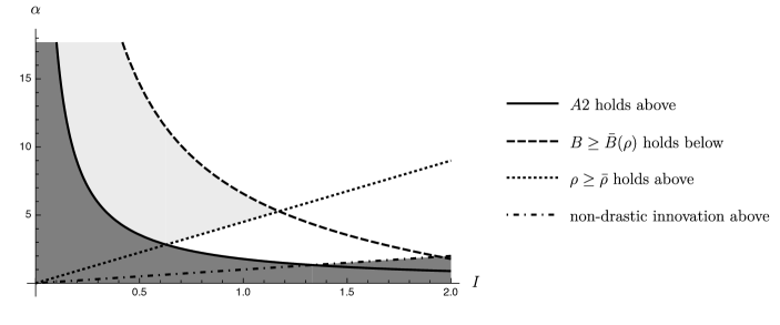
Figure 3: Comparison of R&D competition and RJV in a Cournot example with inverse demand $P(Q)=a-bQ$, constant marginal costs $c$, $B=0.01$, $\rho=0.1$ and $C(\theta)=\frac{\theta}{1-\theta^{2}}$. Axes depict cost reduction $I$ and $\alpha=a-c$.

Thus, after calculating $\overline{\rho}=\frac{I}{2\alpha+I}$, we directly obtain:

Corollary 1.

In the linear Cournot model, the innovation probability is strictly higher with an RJV than with R&D competition if and only if $\rho>\bar{\rho}=\frac{I}{2\alpha+I}$ and $B>\bar{B}(\rho)$. If these conditions both hold, then the total R&D expenditures of the RJV are lower than those under R&D competition.

When competition is moderate or intense, the RJV only improves the innovation probability if the impact of pooling of resources is significant enough (as captured by the conditions on $\rho$ and B). Importantly, Corollary 1 also identifies the role of the product market. A larger product market (captured by higher $\alpha$) and a smaller innovation size $I$ both increase the range of interest rates for which the RJV increases profits.

Figure 3 illustrates the result for specific parameter values. Assumption 1 and the focus on non-drastic innovations imply that we do not consider the darkly shaded region. The lightly shaded area depicts the parameter region for which the innovation probability is higher with an RJV than with R&D competition. The existence of this region means that the requirement of Assumption 1 that the budget is sufficiently small and the requirement from Proposition 1(ii) that it is sufficiently large are consistent. Note that all RJVs that increase the innovation probability compared to any equilibrium under R&D competition are profitable in this case. In the parameter region colored in white, an RJV lowers the innovation probability compared to any equilibrium under competition.

3.6.2 Differentiated Price Competition

The linear homogeneous Cournot model is simple to analyze, but it restricts the possible outcomes, because competition is moderate or intense, so that Propositions 1(i) and 3(i) never apply. With differentiated goods, competition can be soft (as well as moderate or intense), so that these results become applicable. To see this, consider a standard model of differentiated price competition with inverse demand $p_{i}=1-q_{i}-bq_{j}$ for $b\in[0,1)$ and constant marginal cost $c>0$ where firms can engage in cost reductions $I\leq c$. In the appendix, we derive the equilibrium profits.

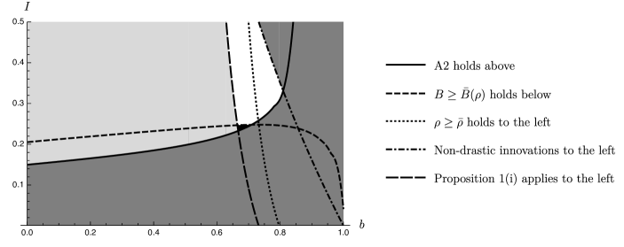
Figure 4: Comparison of R&D competition and RJV in a differentiated Bertrand example with inverse demands $p_{i}=1-q_{i}-bq_{j}$ and constant marginal costs $c=0.5$. Axes depict substitution parameter $b$ and cost reduction $I$.

Figure 4 illustrates the stark contrast to the homogeneous Cournot example. We exclude parameter areas where the innovation is drastic (in which case $\pi_{\mathit{0}I}$ would be negative) and/or Assumption 1 is violated (darkly shaded region). The central observation is that the RJV increases innovation and is profitable with sufficiently weak competition (in the large shaded grey area). This follows by applying Propositions 1(i) and 3(i). By contrast, the parameter region where Proposition 1(ii) and 3(ii) apply is very small (only the very small black area in the middle of the figure). Finally, note that, by Proposition 4, it will be profitable to engage in RJVs that reduce innovation (and costs) for parameter constellations near the left boundary of the white region.

4 Further Results

In this section, we provide further results. We first compare the effects of RJVs with those of mergers. Then we allow for spillovers and licensing, respectively. Finally, we consider markets with more than two firms.

4.1 Mergers vs. RJVs

Competition policy usually views RJVs more favorably than full mergers as they allow the participants to reap some of the efficiency benefits that might arise in R&D, without necessarily eliminating product market competition between the firms involved. However, a precise comparison needs to take differences in the effects of RJVs and mergers on innovation into account. In the following, we therefore analyze the innovation effects of a merger between the two firms, following the above analysis of the RJV closely. Contrary to the RJV, the merged entity not only combines the research budget, but its constituent parts give up competition entirely. We denote the (monopoly) profit of the merged firm as $\pi_{t_{m}}$, where $t_{m}\in\{0,I\}$ indicates whether the firm has successfully innovated or not. In line with Assumption 1(ii), we assume that innovation increases profits.

Assumption 1.

$\pi_{I}>\pi_{\mathit{0}}$.

The analysis for the merged firm is entirely analogous to the RJV case, except that we have to replace $\pi_{II}$ with $\pi_{I}$ and $\pi_{\mathit{0}\mathit{0}}$ with $\pi_{\mathit{0}}$ in the expected payoff formula (1).

Accordingly, we define critical values $\theta^{u}_{m}$ and $\theta^{\rho}_{m}<\theta^{u}_{m}$ which are analogous to $\theta^{u}$ and $\theta^{\rho}$, except that we replace $2[\pi_{II}-\pi_{\mathit{0}\mathit{0}}]$ with $\pi_{I}-\pi_{\mathit{0}}$. It is straightforward that the merged firm optimally uses a single cut-off strategy like the RJV, with $\theta^{u}_{m}$ and $\theta^{\rho}_{m}$ instead of $\theta^{u}$ and $\theta^{\rho}$ (see Lemma 6 in Appendix A.7.1). As a result, the comparison between investments with a merger and with R&D competition (see Proposition 1 in Appendix A.7.1) is analogous to the comparison between the RJV and R&D competition (Proposition 1), except that we again need to replace $2[\pi_{II}-\pi_{\mathit{0}\mathit{0}}]$ with $\pi_{I}-\pi_{\mathit{0}}$, and the interest rate threshold thus becomes

$$\bar{\rho}_{m} =\dfrac{\pi_{I\mathit{0}}-\pi_{\mathit{0}\mathit{0}}-(\pi_{I}-\pi_{\mathit{0}})}{\pi_{I}-\pi_{\mathit{0}}}.$$

The following result compares the innovation probability under a merger and under an RJV.

Proposition 1 (Comparison of an RJV and a merger).

1. If $2[\pi_{II}-\pi_{\mathit{0}\mathit{0}}]\geq\pi_{I}-\pi_{\mathit{0}}$, the innovation probability under an RJV is weakly higher than under a merger. The difference is strict, except when $\theta^{B}\in[\theta^{\rho},\theta^{u}_{m}]$ or $2[\pi_{II}-\pi_{\mathit{0}\mathit{0}}]=\pi_{I}-\pi_{\mathit{0}}$.

2. If $2[\pi_{II}-\pi_{\mathit{0}\mathit{0}}]<\pi_{I}-\pi_{\mathit{0}}$, the innovation probability under an RJV is weakly lower than under a merger. The difference is strict, except when $\theta^{B}\in[\theta^{\rho}_{m},\theta^{u}]$.

A merger leads to similar efficiency gains as an RJV – in both cases duplicate projects are eliminated, and those resources can be invested into new projects. However, the total profit increase for the members of the RJV will generally differ from those for the merged firm: Whereas innovation increases the joint profit of the RJV by $2[\pi_{II}-\pi_{\mathit{0}\mathit{0}}]$, the corresponding value for the merged firm is $\pi_{I}-\pi_{\mathit{0}}$. The above result confirms the intuition that the relative size of these two profit differentials determines whether an RJV or a merged firm will be more likely to generate innovation.

However, there is a subtle effect of financial constraints: Even when the total profit effects of innovation differ for RJVs and mergers, the investments and thus the innovation probability are the same for non-degenerate parameter ranges. This happens when the budgets are intermediate, that is either $\theta^{B}\in[\theta^{\rho},\theta^{u}_{m}]$ in case $(i)$ or $\theta^{B}\in[\theta^{\rho}_{m},\theta^{u}]$ in case $(ii)$. In those cases, both the RJV and the merged firm invest their entire budgets, but the marginal return of additional research projects is not sufficient to justify the cost of borrowing from the capital market. Hence, the RJV and the merged entity each invest exactly the total research budget $2B$ into R&D.

Proposition 1 enables us to analyze whether a merger or an RJV would be better from the consumer surplus perspective, assuming that firms would want to engage in it. Analogously to Proposition 2, we maintain the following weak assumptions: (a) When technology is the same, consumer surplus is higher with two active firms than with one; (b) for the same number of active firms, consumer surplus is higher if the firms have innovated than if they have not. Thus, in case $(i)$ of Proposition 1, the RJV unambiguously increases consumer surplus. The reason is that the RJV both weakly increases the probability that the innovation will be discovered and increases competition for any level of technology. Even in case $(ii)$, where the profit increase from innovation is larger for the merger than for the RJV, the RJV unambiguously leads to higher consumer surplus than the merger if $\theta^{B}\in[\theta^{\rho}_{m},\theta^{u}]$, as the innovation probability is the same for both forms of cooperation. In case $(ii)$, if $\theta^{B}\not\in[\theta^{\rho}_{m},\theta^{u}]$, the comparison is ambiguous: The merged firm would be more likely to discover the innovation, while the RJV would maintain the more competitive market structure. One consequence of this analysis is that from a consumer perspective, an RJV is preferable to a merger, except possibly when the innovation probability would be significantly higher under a merger. This suggests that firms should not only be required to show that a merger would have positive innovation effects, but also that these effects would not occur with an RJV.

4.2 Spillovers

Our model differs from the previous literature on RJVs not only by its focus on financial constraints as opposed to spillovers, but also by the feature that firms can choose between different R&D projects. To simplify the comparison with the existing literature, we first consider a variant of our project choice model without financial constraints, but with spillovers. Thereafter, we analyze the interaction between financial constraints and spillovers.

4.2.1 Spillovers without financial constraints

We modify the setting of Section 2 by assuming that the firms with cost functions $C(\theta)$ choose their investment portfolio without any budget constraint. Moreover, with R&D competition, if a firm has invested successfully in a project and the rival has not, then with probability $\sigma\in[0,1]$ the rival will obtain access to the innovation. Thus, it is now possible that a firm obtains the innovation without investing itself.

We provide the equilibrium characterization for R&D competition in Appendix A.8.1. As in the benchmark model, we obtain an equilibrium in double cut-off strategies. A full description of the equilibrium is given in Lemma 8. The analysis with RJVs is simpler than in the case with financial constraints. The increase in joint profit from a successful innovation is $2\pi_{II}-2\pi_{\mathit{0}\mathit{0}}$. Hence, the RJV invests in all projects up to a cut-off value, which is given by $\theta^{u}$, and it does not invest in the remaining ones. The following result compares investments in the RJV with those under R&D competition.

Proposition 2.

Consider the model with spillovers, but without financial constraints. Assume that $\pi_{I\mathit{0}}>\pi_{II}$. Then the innovation probability is strictly larger under the RJV than under R&D competition if and only if

$$\sigma>1-\frac{\pi_{II}-\pi_{\mathit{0}\mathit{0}}}{\pi_{I\mathit{0}}-\pi_{II}}.$$

This condition is always satisfied if competition is soft.

The proof is in Appendix A.8.1. As in the case with financial constraints, for RJVs to generate a higher innovation probability than R&D competition, it is crucial that the value of escaping competition is sufficiently small relative to the value of joint innovation. A simple, but important implication of Proposition 2 needs to be emphasized: When competition is soft, then the RHS of the inequality in Proposition 2 is negative and an RJV increases innovation for any level of spillovers (including $\sigma=0)$. When competition is moderate or intense, the RHS is positive, but an RJV can still increase the innovation probability if the spillovers are strong enough relative to the strength of the competition. The exception is (homogeneous) Bertrand competition, which is so intense that $\pi_{II}=\pi_{\mathit{0}\mathit{0}}=0$, so that the inequality cannot be satisfied for any $\sigma\in[0,1]$.

4.2.2 Spillovers with financial constraints

In Appendix A.8.2, we integrate the model with spillovers just discussed into the model with financial constraints. Large parts of the analysis follow directly from our results in Section 3. To apply those results, one needs to define the expected payoffs $\tilde{\pi}_{t_{i}t_{j}}$ of discovering the innovation (i.e., before any spillovers happen and taking into account the possibility of a spillover) and then observe that Assumption 1 holds with $\pi$ replaced by $\tilde{\pi}$. Then, the results of Section 3 apply after replacing realized product market profits with expected payoffs. Adapting Assumption 1, we assume that the research budgets of the individual firms are sufficiently small that they will borrow positive amounts in any equilibrium. It is straightforward to show that there is an equilibrium in double cut-off strategies under R&D competition (see Lemma 9 in Appendix A.8.2 for details). The comparison between R&D competition and RJV is also very similar to the case without spillovers (see Proposition 2 in Appendix A.8.2): When the total profit increase $2\pi_{II}-2\pi_{\mathit{0}\mathit{0}}$ from innovation is high enough, then the RJV will lead to a greater innovation probability than R&D competition independent of financial constraints. If the total profit increase from innovation is lower, the RJV only leads to a greater innovation probability if both the interest rate $\rho$ and the RJV budget $2B$ are above a threshold; in this case, the RJV saves investment costs by avoiding duplication.

The following differences to the benchmark model are relevant for the comparison between investments under R&D competition and under the RJV. First, RJVs unconditionally increase innovation whenever $2\pi_{II}-2\pi_{\mathit{0}\mathit{0}}>\pi_{I\mathit{0}}-\pi_{\mathit{0}\mathit{0}}-\sigma(\pi_{I\mathit{0}}-\pi_{II})$, which is more likely to be satisfied when spillovers are strong (i.e., when $\sigma$ is high). Second, when that condition is not satisfied, an increase in $\sigma$ lowers the thresholds for the budget and the interest rate which are needed to guarantee that the RJV increases the innovation probability. The conditions under which an RJV increases the innovation probability are thus weaker with higher spillovers, just as they are with higher interest rates:

Proposition 3 (Benefit of RJV increases in the spillover rate).

Fix any $\sigma$ and $\rho$. If the innovation probability is strictly larger under the RJV than under R&D competition, then it is also strictly larger for any $\sigma^{\prime}\geq\sigma$ and $\rho^{\prime}\geq\rho$.

As in the case without spillovers, an RJV results in efficiency gains at the investment stage by reducing duplication, and resources can be invested in a larger set of projects. Moreover, whereas spillover effects reduce investment under competitive R&D, this is not the case with an RJV. Thus, the positive effect of R&D cooperation on the innovation probability must be larger with spillovers than without, reflecting the internalization of positive spillovers by the RJV.

4.3 Licensing

Like research joint ventures, licensing agreements are an instrument for firms to share the fruits of innovation. The literature has demonstrated the possible benefits and costs of such agreements when R&D efforts are one-dimensional. Here, we show how the possibility of licensing influences R&D project choice in the absence of an RJV and, thereby, the effects of switching to an RJV. In particular, we will show that even when licensing of innovations is possible, RJVs can still lead to an increase in the innovation probability.

We thus extend our benchmark model to allow for licensing of innovations. We suppose that, if only one firm has innovated successfully, it can license the innovation to the competitor with a two-part tariff $(L,\eta)$, consisting of an output-independent fixed fee $L$ and a variable, output-dependent part $\eta$ (e.g., royalties). When the unsuccessful firm licenses the innovation, both the innovator and the licensee have the technology state $t_{i}=I$. However, the incentives of the licensee to compete vigorously are dampened by the variable part of the licensing contract $\eta$. This reduction of the intensity of competition increases total industry profits (compared to the situation when both firms independently innovate) by some amount $\Delta\geq 0$.

We assume that the innovator makes a take it or leave it offer, extracting all the rents from the licensee. In particular, the innovator sets the fixed fee $L$ such that the unsuccessful firm earns its outside option $\pi_{\mathit{0}I}$ and, thus, is indifferent between accepting the contract or not. Therefore, the innovator is willing to license the innovation if her profits with licensing, $2\pi_{II}+\Delta-\pi_{\mathit{0}I}$, are at least as high as her profits without, $\pi_{I\mathit{0}}$. Licensing always happens if competition is soft or moderate and sometimes when it is intense. As in the analysis of spillovers in Section 4.2.2, after replacing the function $\pi_{t_{i}t_{j}}$ appropriately, the analysis directly follows Section 3. Specifically, we define a function $\pi^{L}$ on $\{0,I\}\times\{0,I\}$, which is identical with $\pi$ except that it takes into account licensing payments when only one firm is successful. The only difference between $\pi^{L}$ and $\pi$ is that $\pi^{L}_{I\mathit{0}}=\max\{\pi_{I\mathit{0}},2\pi_{II}+\Delta-\pi_{\mathit{0}I}\}$. This function captures profits as a function of technology level, but taking into account possible gains from licensing. Using this modified profit function, we derive thresholds $\theta^{L}_{1}$ and $\theta^{L}_{2}$ by replacing $\pi$ with $\pi^{L}$ in the definitions of $\theta_{1}$ and $\theta_{2}$. Crucially, whereas $\theta^{L}_{2}=\theta_{2}$, $\theta^{L}_{1}\geq\theta_{1}$, reflecting the potential gains from licensing.

When $2\pi_{II}+\Delta-\pi_{\mathit{0}I}<\pi_{I\mathit{0}}$, the equilibrium under R&D competition is exactly the same as in Lemma 1, because licensing never occurs in this case. When $2\pi_{II}+\Delta-\pi_{\mathit{0}I}\geq\pi_{I\mathit{0}}$, licensing increases the innovation probability in any equilibrium to $\theta_{1}^{L}\geq\theta_{1}$, as the opportunity to license increases the incentives to explore further projects.

For the comparison with the RJV, we replace the budget threshold $\bar{B}(\rho)$ and the interest threshold $\bar{\rho}$ with thresholds $\bar{B}^{L}(\rho)$ and $\bar{\rho}^{L}$ that are based on $\pi^{L}$ rather than $\pi$, leading to the following modification of Proposition 1.

Proposition 4 (Comparison of R&D competition with licensing and RJV).

1. Suppose $2\pi_{II}+\Delta-\pi_{\mathit{0}I}\geq\pi_{I\mathit{0}}$. Then:
   (a) The innovation probability is strictly larger under the RJV than under competition if and only if $B>\bar{B}^{L}(\rho)$ and $\rho>\bar{\rho}^{L}$.
   (b) If the formation of the RJV strictly increases the innovation probability, then it weakly decreases total R&D spending.

2. Suppose $2\pi_{II}+\Delta-\pi_{\mathit{0}I}<\pi_{I\mathit{0}}$. Then the effect of an RJV on the innovation probability is the same as in the absence of a licensing possibility.

In case $(i)$, firms want to license the innovation. In case $(ii)$, they do not. Importantly, the conditions under which the RJV leads to a higher innovation probability are more rigid than without licensing. This is obvious in the case of soft competition, in which Proposition 1(i) states that an RJV is always preferable to R&D competition, while Proposition 4(i) requires that $B>\bar{B}^{L}(\rho)$ and $\rho>\bar{\rho}^{L}$. When competition is not soft, the conditions under which an RJV increases the innovation probability are also more restrictive with licensing than without, since $\bar{B}^{L}(\rho)\geq\bar{B}(\rho)$ and $\bar{\rho}^{L}\geq\bar{\rho}$ whenever Proposition 4(i) applies. The difference arises because licensing increases innovation incentives under R&D competition, so that there is less to gain from an RJV. Moreover, an RJV that increases the innovation probability weakly decreases total R&D spending, because it invests weakly less than the available budget while both firms invest strictly more than their budget under R&D competition.

To put the results into perspective, we can think of ex-post licensing and RJVs as imperfect substitutes for sharing the fruits of R&D. Nonetheless, the above results show that even when ex-post licensing is possible, an RJV may still lead to a higher innovation probability than R&D competition if financial constraints are sufficiently tight.

4.4 Multiple firms

We extend our model by allowing for more than two competing firms. With multiple firms, there are many conceivable ways in which RJVs could be formed, including industry-wide RJVs as well as several competing RJVs. We analyze two illustrative cases. First, we consider a market with three firms that can form an industry-wide RJV. Second, we consider the case of four firms that form two competing RJVs. The analysis is very similar to the benchmark model with two firms. Therefore, we defer details to the Appendix A.9.

4.4.1 Industry-wide RJV

We extend the analysis to the case of three firms, which can form one RJV. Suitably adjusting Assumptions 1 and 1, the analysis and results are analogous to the benchmark model with two firms. The only notable difference is that the R&D competition game now has multiple equilibria in triple cut-off strategies characterized by the three critical values $\theta_{3}\leq\theta_{2}\leq\theta_{1}$. However, the innovation probability in any equilibrium is still given by $\theta_{1}$, the most expensive project in which a single firm can profitably invest relying on external resources. The analysis of the RJV when all firms participate and the resulting comparison between R&D competition and cooperation is qualitatively unchanged. Therefore, we find similar results to Proposition 1: When competition is not too intense, the innovation probability is higher in the RJV; otherwise, this conclusion requires the budget and the external financing costs to be high enough. In the latter case, total R&D-spending in the RJV is lower than under competition.

4.4.2 Multiple RJVs

Next, we consider the formation of multiple RJVs. We consider a market with four firms that form two symmetric RJVs, each with two firms. Therefore, R&D cooperation does not eliminate competition in the innovation stage entirely, but reduces the number of competing agents. Hence, even with an RJV cheap projects are still duplicated. We assume that the budget of an RJV is sufficiently large that it never borrows in equilibrium. Otherwise, the analysis of two competing RJVs turns out to be similar to the R&D competition regime in the baseline model. Analogously to Proposition 1, we find: When competition is relatively soft, then the innovation probability is higher with two RJVs than with R&D competition without additional conditions. Under relatively moderate or intense competition, cooperation on R&D increases the innovation probability only if the budget and the interest rate are sufficiently high. In this case, total R&D-spending with two RJVs is lower than when four firms invest individually.

5 Relation to the Literature

Our paper analyzes R&D competition between duopolists who (i) select between different R&D projects and (ii) are financially constrained. It compares their R&D decisions with those of research joint ventures and merged firms. Accordingly, we briefly discuss the relation of our paper to existing treatments of R&D project choice, financially constrained oligopolists, research joint ventures and mergers and innovation.

Innovation project choice: Our model of R&D competition with project choice builds on Letina (2016) who also considers symmetric incumbents. Letina et al. (2021) apply that framework to study the innovation decisions of asymmetric firms (an incumbent and an entrant). These papers neither include financial constraints, nor do they address joint ventures. Contrary to these models, Moraga-González et al. (2022) allow for (two) different types of R&D, but fix the overall spending.

Financially constrained firms: Authors such as Hall and Lerner (2010) and Kerr and Nanda (2015) have stated several reasons why external financing of R&D investments is more costly than for other investments. As a result, internal financing plays a strong role (Czarnitzki and Hottenrott (2011)). Several authors have provided empirical evidence that financial constraints have a negative impact on R&D investment (Mohnen et al. (2008), Savignac (2008), Mancusi and Vezzulli (2014), Howell (2017) Krieger et al. (2022), Caggese (2019)). In line with our Propositions 3 and 4, Sovinsky (2022) finds that capital-constrained firms are more likely to join an RJV. While the empirical literature on financially constrained firms is voluminous, the theoretical literature is small. We are not aware of any oligopoly model of financially constrained firms (with or without RJV formation) that choose how much as well as in which projects to invest.

The theory of research joint ventures: Our paper differs from the existing theoretical literature on RJVs in two important dimensions. First, the literature does not allow for different R&D projects. Second, it does not model the role of financial constraints. Instead, it focuses mainly on spillovers. Without RJVs, as in our model, firms invest in R&D to gain a competitive advantage over their rivals. However, if knowledge spillovers to competitors are large enough, such gains are small and firms limit their R&D investments. Accordingly, d’Aspremont and Jacquemin (1988) show in a static, two-stage, duopolistic Cournot model that, with high spillovers, an RJV leads to larger R&D expenditures, more output and higher welfare than R&D competition. By contrast, with low spillovers, welfare under R&D competition is higher than in an RJV, as an RJV would lower total R&D investments. As argued above, we find that, with soft competition (for instance, with sufficiently differentiated price competition), an RJV increases the investment probability (and hence welfare) even with low spillovers. Like our paper, Katz (1986) and Kamien et al. (1992) show how the nature of product market competition affects the comparison between R&D competition and cooperation. Like other authors, such as Amir et al. (2019), both papers also argue that an RJV reduces wasteful effort duplication. However, contrary to our approach, none of these papers explicitly models duplication in the natural setting where firms can select between different projects. Instead, firms can only choose the amount of R&D investment, which is in a strictly positive relation with the R&D outcome (the size or probability of an innovation). In our model, an RJV may well increase the innovation probability while investing less resources because duplication is eliminated. This feature is particularly relevant when there is fundamental uncertainty about the right approach to R&D. The literature has also highlighted important caveats to the claim that research cooperation is socially beneficial: RJVs foster product market collusion, which leads to dynamic inefficiency (Grossman and Shapiro (1986), Martin (1996), Jacquemin (1988), Caloghirou et al. (2003) and Miyagiwa (2009)). Competition authorities who decide on such RJVs have to weigh these risks against the potential benefits, which is difficult given realistic informational constraints (Cassiman, 2000).

The empirics of research joint ventures: Empirical studies support the claims of the theoretical literature. Cassiman and Veugelers (2002) show that Belgian manufacturing firms are more likely to cooperate when spillovers are high. Aschhoff and Schmidt (2008) show that R&D cooperation among competitors reduces production costs. Becker and Dietz (2004) provide empirical evidence that members of an RJV invest more in research than without cooperation, and that they are more likely to obtain new products. Veugelers (1997) also finds that cooperation increases investments, but that this requires absorptive capacity. Further, she concludes that firms are more likely to join an RJV the more they spend on R&D. Röller et al. (2007) show that cost-sharing motives are important for RJV formation. Link (1998) provides case-study evidence for efficiencies in a specific RJV. Finally, Duso et al. (2014) and Sovinsky (2022) find empirical evidence that RJVs among competitors are more prone to collusion, which reduces welfare. Thus, horizontal R&D cooperation should come under scrutiny by authorities.

Mergers and innovation: Several authors have recently studied under which circumstances incumbent mergers increase innovation. Federico et al. (2017, 2018) and Motta and Tarantino (2021) identify negative effects in models with one-dimensional R&D effort; similarly, Letina (2016) and Gilbert (2019) obtain negative effects on R&D diversity in models of project choice. Denicolò and Polo (2018) find positive effects. In Bourreau et al. (2021), both possibilities arise, where the positive effects come from allowing for horizontal rather than only vertical R&D innovations. In our model with project choices of financially constrained firms who engage in purely vertical innovations, we similarly find that the effects of the merger can be positive or negative. Contrary to Bourreau et al. (2021), however, the possibility of a positive effect reflects the merged entity’s ability to coordinate which projects to invest in and the existence of financial constraints. Moreover, which effect occurs depends on the intensity of product market competition.

6 Conclusion

This paper provides a novel theory of research joint ventures for financially constrained firms who can choose the set of research projects that they will pursue. Research joint ventures allow firms to share their R&D budget and to coordinate their R&D investment decisions, while maintaining product market competition.

We find that, if product market competition is sufficiently soft, the RJV will increase the probability of an innovation even when there are no financial constraints. As product market competition increases, a positive innovation effect of the RJV requires that the external funding conditions are sufficiently bad and the budget of the RJV is sufficiently large. In the latter case, the RJV reduces research costs by avoiding duplication – this shows that the relation between R&D spending and R&D success probability need not be positive. Moreover, any RJV that increases the innovation probability also increases expected consumer welfare.

Importantly, the conditions under which the RJV increases the probability of a successful innovation and the conditions under which it is profitable for the participants often coincide; in particular, for soft or intermediate competition, firms always want to form RJVs if they increase the innovation probability. This increases consumer welfare under mild conditions. Nonetheless, we also identify situations under which firms find it profitable to form an innovation-reducing RJV merely because they can coordinate on reducing R&D costs, which is in line with concerns of policy makers.

We obtain qualitatively similar results on the effects of mergers on innovation. More interestingly, we find conditions under which a merger does not lead to a lower innovation probability than an RJV. In such situations, even if the merger has pro-competitive effects on innovation relative to the benchmark of R&D competition, the merger should be prohibited because, contrary to the alternative of an RJV, it results in an adverse effect on product market competition.

Appendix A Proofs

A.1 Proof of Lemma 1

We will first prove an intermediate result.

Lemma 1.

Any strategy $r_{i}$ such that $\int_{0}^{1}r_{i}(\theta)C(\theta)d\theta\leq B$ is dominated.

Proof.

If $\int_{0}^{1}r_{i}(\theta)C(\theta)d\theta\leq B$, then by Assumption 1 there exists a set $\Theta^{\prime}\subseteq[0,\theta_{2})$ of positive measure, such that $r_{i}(\theta)=0$ for all $\theta\in\Theta^{\prime}$. Consider a strategy $r^{\prime}_{i}$, where $r^{\prime}_{i}(\theta)=1$ for all $\theta\in[0,\theta_{2})$ and $r^{\prime}_{i}(\theta)=r_{i}(\theta)$ otherwise. We will show that $\mathbb{E}\Pi_{i}(r_{i}^{\prime},r_{j})>\mathbb{E}\Pi_{i}(r_{i},r_{j})$ for any strategy of the opponent $r_{j}$.

Noting that the strategy $r_{i}^{\prime}$ requires external financing (while $r_{i}$ does not), and taking into account that $r^{\prime}_{i}(\theta)=r_{i}(\theta)$ for all $\theta>\theta_{2}$ then

$$\mathbb{E}\Pi_{i}(r_{i}^{\prime},r_{j})-\mathbb{E}\Pi_{i}(r_{i},r_{j})=$$

$$\int_{0}^{\theta_{2}}(r_{i}^{\prime}(\theta)-r_{i}(\theta))\Big{[}(1-r_{j}(\theta))\left[\pi_{I\mathit{0}}-\pi_{\mathit{0}\mathit{0}}\right]+r_{j}(\theta)\left[\pi_{II}-\pi_{\mathit{0}I}\right]\Big{]}d\theta$$

$$-(1+\rho)\int_{0}^{1}r_{i}^{\prime}(\theta)C(\theta)d\theta+\rho B+\int_{0}^{1}r_{i}(\theta)C(\theta)d\theta$$

$$\geq\int_{0}^{\theta_{2}}(r_{i}^{\prime}(\theta)-r_{i}(\theta))\Big{[}(1-r_{j}(\theta))\left[\pi_{I\mathit{0}}-\pi_{\mathit{0}\mathit{0}}\right]+r_{j}(\theta)\left[\pi_{II}-\pi_{\mathit{0}I}\right]\Big{]}d\theta$$

$$-(1+\rho)\int_{0}^{1}r_{i}^{\prime}(\theta)C(\theta)d\theta+(1+\rho)\int_{0}^{1}r_{i}(\theta)C(\theta)d\theta$$

$$=\int_{0}^{\theta_{2}}(r_{i}^{\prime}(\theta)-r_{i}(\theta))\Big{[}(1-r_{j}(\theta))\left[\pi_{I\mathit{0}}-\pi_{\mathit{0}\mathit{0}}\right]+r_{j}(\theta)\left[\pi_{II}-\pi_{\mathit{0}I}\right]\Big{]}d\theta$$

$$-(1+\rho)\int_{0}^{\theta_{2}}(r_{i}^{\prime}(\theta)-r_{i}(\theta))C(\theta)d\theta$$

$$\geq\int_{0}^{\theta_{2}}(r_{i}^{\prime}(\theta)-r_{i}(\theta))\Big{[}\left(\pi_{II}-\pi_{\mathit{0}I}\right)-(1+\rho)C(\theta)\Big{]}d\theta$$

$$>0.$$

The first inequality follows from the assumption that $\int_{0}^{1}r_{i}(\theta)C(\theta)d\theta\leq B$, the second from the fact that $\pi_{I\mathit{0}}-\pi_{\mathit{0}\mathit{0}}\geq\pi_{II}-\pi_{\mathit{0}I}$ and $r_{i}^{\prime}(\theta)-r_{i}(\theta)\geq 0$ and the last from the fact that $\pi_{II}-\pi_{\mathit{0}I}>(1+\rho)C(\theta)$ for all $\theta<\theta_{2}$ and $r_{i}^{\prime}(\theta)>r_{i}(\theta)$ on the set of positive measure $\Theta^{\prime}$. ∎

Proof of (i): Take any strategy $r_{j}$ which corresponds to one of the equilibrium strategies given in Lemma 1. Note that for any fixed $r_{j}$, the equilibrium candidate strategy $r_{i}$ is uniquely determined. Suppose $(r_{i},r_{j})$ does not constitute an equilibrium. Then, there exists a strategy $r^{\prime}_{i}$ such that $\mathbb{E}\Pi_{i}(r_{i}^{\prime},r_{j})>\mathbb{E}\Pi_{i}(r_{i},r_{j})$. By Assumption 1, all equilibrium candidates satisfy $\int_{0}^{1}r_{i}(\theta)C(\theta)d\theta>B$. Moreover, by Lemma 1 we can focus on strategies such that $\int_{0}^{1}r^{\prime}_{i}(\theta)C(\theta)d\theta>B$ is satisfied.

Denote the expected total payoff of project $\theta$, conditional on it being correct, as $v_{i}(\theta,r_{i},r_{j})$. Then there exists a set $\Theta^{\prime}\subseteq[0,1)$ with positive measure such that $v_{i}(\theta,r^{\prime}_{i},r_{j})>v_{i}(\theta,r_{i},r_{j})$ for all $\theta\in\Theta^{\prime}$, or more explicitly:

$$(1-r_{j}(\theta))[r^{\prime}_{i}(\theta)\pi_{I\mathit{0}}+(1-r^{\prime}_{i}(\theta))\pi_{\mathit{0}\mathit{0}}]+r_{j}(\theta)[r^{\prime}_{i}(\theta)\pi_{II}+(1-r^{\prime}_{i}(\theta))\pi_{\mathit{0}I}]$$

$$-(1+\rho)C(\theta)r^{\prime}_{i}(\theta)>(1-r_{j}(\theta))[r_{i}(\theta)\pi_{I\mathit{0}}+(1-r_{i}(\theta))\pi_{\mathit{0}\mathit{0}}]$$

$$+r_{j}(\theta)[r_{i}(\theta)\pi_{II}+(1-r_{i}(\theta))\pi_{\mathit{0}I}]-(1+\rho)C(\theta)r_{i}(\theta).$$ (3)

If $\theta<\theta_{2}$ then $r_{j}(\theta)=1$ so this inequality simplifies to

$$\begin{split}r^{\prime}_{i}(\theta)(\pi_{II}-\pi_{\mathit{0}I}-(1+\rho)C(\theta))>r_{i}(\theta)(\pi_{II}-\pi_{\mathit{0}I}-(1+\rho)C(\theta))\end{split}$$ (4)

Since for $\theta<\theta_{2}$ we have $\pi_{II}-\pi_{\mathit{0}I}-(1+\rho)C(\theta)>0$ and $r_{i}(\theta)=1$, this would imply $r^{\prime}_{i}(\theta)>1$ which is a contradiction.

If $\theta>\theta_{1}$ then $r_{j}(\theta)=0$ so inequality (A.1) simplifies to

$$r^{\prime}_{i}(\theta)[\pi_{I\mathit{0}}-\pi_{\mathit{0}\mathit{0}}-(1+\rho)C(\theta)]>r_{i}(\theta)[\pi_{I\mathit{0}}-\pi_{\mathit{0}\mathit{0}}-(1+\rho)C(\theta)].$$ (5)

Since for $\theta>\theta_{1}$ we have $\pi_{I\mathit{0}}-\pi_{\mathit{0}\mathit{0}}-(1+\rho)C(\theta)<0$ and $r_{i}(\theta)=0$ this would imply $r^{\prime}_{i}(\theta)<0$ which is a contradiction.

Next, consider $\theta\in(\theta_{2},\theta_{1})$. This case only arises if $\theta_{2}<\theta_{1}$, which immediately implies $\pi_{I\mathit{0}}+\pi_{\mathit{0}I}-\pi_{II}-\pi_{\mathit{0}\mathit{0}}>0$. If $r_{j}(\theta)=1$ then, as before, inequality (A.1) simplifies to (4). However, now $\pi_{II}-\pi_{\mathit{0}I}-(1+\rho)C(\theta)<0$ and, for the candidate equilibrium, $r_{i}(\theta)=0$. (4) would thus require that $r^{\prime}_{i}(\theta)<0$, which is a contradiction. Similarly if $r_{j}(\theta)=0$ the inequality (A.1) simplifies to (5), but $\theta<\theta_{1}$ implies $\pi_{I\mathit{0}}-\pi_{\mathit{0}\mathit{0}}-(1+\rho)C(\theta)>0$ and, for the candidate equilibrium, $r_{i}(\theta)=1$. (5) would thus require that $r^{\prime}_{i}(\theta)>1$, which is a contradiction.

Proof of (ii): Suppose there exist two strategies, $r_{i}$ and $r_{j}$, which constitute an equilibrium, and a set of positive measure $I\subseteq[0,1)$, such that $r_{i}$ is different from the strategies characterized in the Lemma at all points of the set $I$. By Lemma 1 we can focus on strategies such that the budget is binding. Let $I_{1}=I\cap(0,\theta_{2})$, $I_{2}=I\cap(\theta_{2},\theta_{1})$ and $I_{3}=I\cap(\theta_{1},1)$. Note that at least one of the sets $I_{1}$, $I_{2}$, or $I_{3}$ has positive measure.

Define

$$\Gamma_{i}(\theta,r_{j})= \pi_{I\mathit{0}}-\pi_{\mathit{0}\mathit{0}}-(1+\rho)C(\theta)$$

$$-r_{j}(\theta)(\pi_{I\mathit{0}}+\pi_{\mathit{0}I}-\pi_{II}-\pi_{\mathit{0}\mathit{0}}).$$

We can express $v_{i}(\theta,r_{i},r_{j})$, the expected total payoff of project $\theta$, conditional on it being correct, as

$$v_{i}(\theta,r_{i},r_{j})=r_{i}(\theta)\Gamma_{i}(\theta,r_{j})+(1-r_{j}(\theta))\pi_{\mathit{0}\mathit{0}}+r_{j}(\theta)\pi_{\mathit{0}I}.$$

Since $\pi_{I\mathit{0}}+\pi_{\mathit{0}I}-\pi_{II}-\pi_{\mathit{0}\mathit{0}}\geq 0$, $\Gamma_{i}(\theta,r_{j})$ is decreasing in $r_{j}(\theta)$.

Assume first that $I_{1}$ has positive measure. Then $r_{i}(\theta)=0$ for all $\theta\in I_{1}$. Since $C(\theta)$ is strictly increasing and $(1+\rho)C(\theta_{2})=\pi_{II}-\pi_{\mathit{0}I}$, then $\Gamma_{i}(\theta,r_{j})>0$ for any $r_{j}$. Thus, the best response of firm $i$ is $r_{i}(\theta)=1$ for all $\theta\in I_{1}$, which is a contradiction.

Next, assume $I_{3}$ has positive measure. Then $r_{i}(\theta)=1$ for all $\theta\in I_{3}$. But, analogously to before, $\Gamma_{i}(\theta,r_{j})<0$ for any $r_{j}$. Thus, the best response of firm $i$ is $r_{i}(\theta)=0$. A contradiction.

Finally, assume $I_{2}$ has positive measure, which implies that $r_{i}(\theta)=r_{j}(\theta)$ for all $\theta\in I_{2}$. Suppose first that $r_{i}(\theta)=0$ on a set of positive measure $I_{2}^{\prime}\subseteq I_{2}$. Observe that $\Gamma_{j}(\theta,r_{i})>0$ for all $\theta\in I_{2}^{\prime}$. Since this is an equilibrium, it must be that $r_{j}(\theta)=1$ for all $\theta\in I_{2}^{\prime}$. A contradiction. Next, suppose that $r_{i}(\theta)=1$ on a set of positive measure $I_{2}^{\prime\prime}\subseteq I_{2}$. Observe that $\Gamma_{j}(\theta,r_{i})<0$ for all $\theta\in I_{2}^{\prime\prime}$. Analogously to the argument above, it must be that $r_{j}(\theta)=0$ for all $\theta\in I_{2}^{\prime\prime}$, a contradiction. Thus, it cannot be that $r_{i}(\theta)=r_{j}(\theta)$ for all $\theta\in I_{2}$. ∎

A.2 Proof of Lemma 2

We can rewrite the expected total payoff of the RJV as

$$\mathbb{E}\Pi_{v}(r_{v})=2 \pi_{\mathit{0}\mathit{0}}+2\left[\pi_{II}-\pi_{\mathit{0}\mathit{0}}\right]\int_{0}^{1}r_{v}(\theta)d\theta$$

$$-\int_{0}^{1}r_{v}(\theta)C(\theta)d\theta-\rho\max\left\{\int_{0}^{1}r_{v}(\theta)C(\theta)d\theta-2B,0\right\}$$

where the probability that the RJV discovers the innovation is given by $\int_{0}^{1}r_{v}(\theta)d\theta$ while $\int_{0}^{1}r_{v}(\theta)C(\theta)d\theta+\rho\max\left\{\int_{0}^{1}r_{v}(\theta)C(\theta)d\theta-2B,0\right\}$ captures total innovation costs.

Since research projects only differ with respect to investment costs and these costs are increasing in $\theta$, for any fixed probability of innovation $\hat{\theta}$, the RJV optimally chooses a cut-off strategy to obtain this probability: It sets $r_{v}(\theta)=1$ for $\theta<\hat{\theta}$ and $r_{v}(\theta)=0$ otherwise, so that $\int_{0}^{1}r_{v}(\theta)C(\theta)d\theta$=$\int_{0}^{\hat{\theta}}C(\theta)d\theta$.

The RJV’s optimal portfolio can be obtained by maximizing

$$\mathbb{E}\hat{\Pi}_{v}(\hat{\theta})=2\pi_{\mathit{0}\mathit{0}}+2\left[\pi_{II}-\pi_{\mathit{0}\mathit{0}}\right]\hat{\theta}-\int_{0}^{\hat{\theta}}C(\theta)d\theta-\rho\max\left\{\int_{0}^{\hat{\theta}}C(\theta)d\theta-2B,0\right\}.$$

Note that

$$\dfrac{\partial\mathbb{E}\hat{\Pi}_{v}}{\partial\hat{\theta}}=\begin{cases}2\left[\pi_{II}-\pi_{\mathit{0}\mathit{0}}\right]-C(\hat{\theta})&\text{for }\hat{\theta}<\theta^{B}\\ 2\left[\pi_{II}-\pi_{\mathit{0}\mathit{0}}\right]-(1+\rho)C(\hat{\theta})&\text{for }\hat{\theta}>\theta^{B}.\end{cases}$$

Now consider the three cases from the proposition (i.e., whether $\theta^{B}<\theta^{\rho}$, $\theta^{B}\in[\theta^{\rho},\theta^{u}]$, or $\theta^{B}>\theta^{u}$). First, if $\theta^{B}<\theta^{\rho}$ then

$$\dfrac{\partial\mathbb{E}\hat{\Pi}_{v}}{\partial\hat{\theta}}=\begin{cases}2\left[\pi_{II}-\pi_{\mathit{0}\mathit{0}}\right]-C(\hat{\theta})>0&\text{for }\hat{\theta}<\theta^{B}\\ 2\left[\pi_{II}-\pi_{\mathit{0}\mathit{0}}\right]-(1+\rho)C(\hat{\theta})>0&\text{for }\hat{\theta}\in(\theta^{B},\theta^{\rho})\\ 2\left[\pi_{II}-\pi_{\mathit{0}\mathit{0}}\right]-(1+\rho)C(\hat{\theta})<0&\text{for }\hat{\theta}\in(\theta^{\rho},1).\end{cases}$$

Thus, $\hat{\theta}=\theta^{\rho}$ maximizes the expected return of the RJV’s portfolio. Second, if $\theta^{B}\in[\theta^{\rho},\theta^{u}]$ then

$$\dfrac{\partial\mathbb{E}\hat{\Pi}_{v}}{\partial\hat{\theta}}=\begin{cases}2\left[\pi_{II}-\pi_{\mathit{0}\mathit{0}}\right]-C(\hat{\theta})>0&\text{for }\hat{\theta}<\theta^{B}\\ 2\left[\pi_{II}-\pi_{\mathit{0}\mathit{0}}\right]-(1+\rho)C(\hat{\theta})<0&\text{for }\hat{\theta}>\theta^{B},\end{cases}$$

so that $\hat{\theta}=\theta^{B}$ maximizes the expected return of the RJV’s portfolio. Third, if $\theta^{B}>\theta^{u}$ then

$$\dfrac{\partial\mathbb{E}\hat{\Pi}_{v}}{\partial\hat{\theta}}=\begin{cases}2\left[\pi_{II}-\pi_{\mathit{0}\mathit{0}}\right]-C(\hat{\theta})>0&\text{for }\hat{\theta}<\theta^{u}\\ 2\left[\pi_{II}-\pi_{\mathit{0}\mathit{0}}\right]-C(\hat{\theta})<0&\text{for }\hat{\theta}\in(\theta^{u},\theta^{B})\\ 2\left[\pi_{II}-\pi_{\mathit{0}\mathit{0}}\right]-(1+\rho)C(\hat{\theta})<0&\text{for }\hat{\theta}\in(\theta^{B},1).\end{cases}$$

Thus, $\hat{\theta}=\theta^{u}$ maximizes the expected return of the RJV’s portfolio. ∎

A.3 Proof of Proposition 1

First, we provide a lemma distinguishing the two parts of Proposition 1.

Lemma 2.

$2\pi_{II}>\pi_{I\mathit{0}}+\pi_{\mathit{0}\mathit{0}}\Leftrightarrow\theta^{\rho}>\theta_{1}$.

Proof.

$$2\pi_{II} >\pi_{I\mathit{0}}+\pi_{\mathit{0}\mathit{0}}$$

$$2[\pi_{II}-\pi_{\mathit{0}\mathit{0}}] >\pi_{I\mathit{0}}-\pi_{\mathit{0}\mathit{0}}$$

$$(1+\rho)C(\theta^{\rho}) >(1+\rho)C(\theta_{1})$$

$$\theta^{\rho} >\theta_{1}.$$

∎

(i) By Lemma 2, $2\pi_{II}>\pi_{I\mathit{0}}+\pi_{\mathit{0}\mathit{0}}$ implies $\theta^{\rho}>\theta_{1}$. By Lemma 2, the probability that the RJV innovates is at least $\theta^{\rho}$. By Lemma 1, the probability of innovation under competition is $\theta_{1}$. Therefore, the probability that the innovation will be discovered is strictly larger under the RJV than under competition.

(ii) To prove part (a), we first provide an auxiliary result (Lemma 3). Using this lemma, we separately show that “if” part follows from Lemma 4 below and “only if” part from Lemma 5 below.

Lemma 3.

Suppose $2\pi_{II}\leq\pi_{I\mathit{0}}+\pi_{\mathit{0}\mathit{0}}$. Then $\rho>\bar{\rho}\Leftrightarrow\theta^{u}>\theta_{1}$.

Proof.

First suppose that $\bar{\rho}<\infty$. Then

$$\rho >\bar{\rho}=\dfrac{\pi_{I\mathit{0}}-2\pi_{II}+\pi_{\mathit{0}\mathit{0}}}{2[\pi_{II}-\pi_{\mathit{0}\mathit{0}}]}$$

$$2\rho[\pi_{II}-\pi_{\mathit{0}\mathit{0}}] >\pi_{I\mathit{0}}-2\pi_{II}+\pi_{\mathit{0}\mathit{0}}$$

$$2(1+\rho)[\pi_{II}-\pi_{\mathit{0}\mathit{0}}] >\pi_{I\mathit{0}}-\pi_{\mathit{0}\mathit{0}}$$

$$2[\pi_{II}-\pi_{\mathit{0}\mathit{0}}] >\dfrac{\pi_{I\mathit{0}}-\pi_{\mathit{0}\mathit{0}}}{1+\rho}$$

$$C(\theta^{u}) >C(\theta_{1})$$

$$\theta^{u} >\theta_{1}.$$

Next suppose $\bar{\rho}=\infty$. Then, clearly $\rho<\bar{\rho}$. Hence, the statement of the lemma holds if and only if $\theta^{u}\leq\theta_{1}$ or $2[\pi_{II}-\pi_{\mathit{0}\mathit{0}}]\leq\frac{\pi_{I\mathit{0}}-\pi_{\mathit{0}\mathit{0}}}{1+\rho}$. As $\bar{\rho}=\infty$ implies $\pi_{II}=\pi_{\mathit{0}\mathit{0}}$, this requirement holds. ∎

Lemma 4.

Suppose $2\pi_{II}\leq\pi_{I\mathit{0}}+\pi_{\mathit{0}\mathit{0}}$. If $B>\bar{B}(\rho)$ and $\rho>\bar{\rho}$, then the probability that the innovation will be discovered is strictly larger under the RJV than under competition.

Proof.

$B>\int_{0}^{\theta_{1}}C(\theta)d\theta/2$ implies $\int_{0}^{\theta^{B}}C(\theta)d\theta>\int_{0}^{\theta_{1}}C(\theta)d\theta$ and therefore $\theta_{1}<\theta^{B}$. Furthermore, by Lemma 2, $\theta^{\rho}\leq\theta_{1}$ so that $\theta^{\rho}<\theta^{B}$. Then, either $\theta^{B}\in(\theta^{\rho},\theta^{u})$ or $\theta^{B}\geq\theta^{u}$. If $\theta^{B}\in(\theta^{\rho},\theta^{u})$, then the RJV invests in all projects in the set $(0,\theta^{B})$ and discovers the innovation with probability $\theta^{B}$. Without the RJV, in any equilibrium, the firms invest in projects in the set $(0,\theta_{1})$ and the innovation is discovered with probability $\theta_{1}$. Since $\theta^{B}>\theta_{1}$ it immediately follows that the probability of innovation strictly increases under the RJV.

Next, suppose $\theta^{B}\geq\theta^{u}$. Then, the RJV invests in all projects in the set $(0,\theta^{u})$ and discovers the innovation with probability $\theta^{u}$. Since $\rho>\bar{\rho}$ implies $\theta^{u}>\theta_{1}$ by Lemma 3, it follows that the probability of innovation strictly increases under the RJV. ∎

Lemma 5.

Suppose $2\pi_{II}\leq\pi_{I\mathit{0}}+\pi_{\mathit{0}\mathit{0}}$. If the probability that the innovation will be discovered is strictly larger under the RJV than under competition, then $B>\bar{B}(\rho)$ and $\rho>\bar{\rho}$.

Proof.

As $2\pi_{II}\leq\pi_{I\mathit{0}}+\pi_{\mathit{0}\mathit{0}}$, Lemma 2 implies $\theta^{\rho}\leq\theta_{1}$. Hence, if the probability that the innovation will be discovered is strictly larger under the RJV than under competition, then $\theta^{B}>\theta^{\rho}$ by Lemma 2. Therefore, either $\theta^{B}\in(\theta^{\rho},\theta^{u})$ or $\theta^{B}\geq\theta^{u}$. If $\theta^{B}\in(\theta^{\rho},\theta^{u})$, then, by Lemma 2, the increase in the probability of discovering the innovation under the RJV implies $\theta^{B}>\theta_{1}$, so that $\theta^{u}>\theta^{B}>\theta_{1}$. If $\theta^{B}\geq\theta^{u}$, then the increase in the probability of discovering the innovation under RJV implies $\theta^{u}>\theta_{1}$, so that $\theta^{B}\geq\theta^{u}>\theta_{1}$. In either case, both $\theta^{u}>\theta_{1}$ and $\theta^{B}>\theta_{1}$.

Note that $\theta^{B}>\theta_{1}$ implies

$$\int_{0}^{\theta^{B}}C(\theta)d\theta>\int_{0}^{\theta_{1}}C(\theta)d\theta.$$

It follows immediately that $B>\int_{0}^{\theta_{1}}C(\theta)d\theta/2=\bar{B}(\rho)$. Furthermore, $\theta^{u}>\theta_{1}$ implies, by Lemma 3, that $\rho>\bar{\rho}$. ∎

Finally, we prove part (b) of (ii). With moderate or intense competition, $2\pi_{II}\leq\pi_{I\mathit{0}}+\pi_{\mathit{0}\mathit{0}}$. If the formation of the RJV strictly increases the probability of discovering the innovation, then, by Lemma 5, $B>\bar{B}(\rho)$ and $\rho>\bar{\rho}$. Using the same argument as in the proof of Lemma 5, we have that either $\theta^{B}\in(\theta^{\rho},\theta^{u})$ or $\theta^{B}\geq\theta^{u}$. If $\theta^{B}\in(\theta^{\rho},\theta^{u})$, then by Lemma 2, the total costs of the RJV are

$$\int_{0}^{\theta^{B}}C(\theta)d\theta=2B.$$ (6)

If $\theta^{B}\geq\theta^{u}$, then by Lemma 2, the total cost of the RJV are

$$\int_{0}^{\theta^{u}}C(\theta)d\theta\leq 2B.$$ (7)

By Lemma 1, the total costs for equilibrium strategies $r^{*}_{i}$ and $r^{*}_{j}$ under competition are

$$(1+\rho)\int_{0}^{1}[r^{*}_{i}(\theta)+r^{*}_{j}(\theta)]C(\theta) d\theta-2\rho B$$

$$=(1+\rho)\left[2\int_{0}^{\theta_{2}}C(\theta)d\theta+\int_{\theta_{2}}^{\theta_{1}}[r^{*}_{i}(\theta)+r^{*}_{j}(\theta)]C(\theta)d\theta\right]-2\rho B$$

$$>(1+\rho)\left[2B+\int_{\theta_{2}}^{\theta_{1}}[r^{*}_{i}(\theta)+r^{*}_{j}(\theta)]C(\theta)d\theta\right]-2\rho B$$

$$=2B+(1+\rho)\int_{\theta_{2}}^{\theta_{1}}[r^{*}_{i}(\theta)+r^{*}_{j}(\theta)]C(\theta)d\theta$$

$$\geq 2B,$$

where the first inequality follows from Assumption 1, and the second inequality from $\theta_{1}\geq\theta_{2}$ and $r^{*}_{i}(\theta)+r^{*}_{j}(\theta)\geq 0$ for any $\theta$.

It immediately follows that the total cost under competition is weakly larger than the total cost under RJV, which proves the proposition.∎

A.4 Proof of Proposition 2

Denote with $\mathcal{P}^{com}_{II}$ the probability that both firms discover the innovation under competition and with $\mathcal{P}^{com}_{I\mathit{0}}$ the probability that a single firm discovers the innovation under competition. Analogously, let $\mathcal{P}^{rjv}_{II}$ be the probability that the innovation is discovered under the RJV.

The expected consumer surplus is strictly higher under RJV than under competition if

$$\mathcal{P}^{rjv}_{II}CS_{II}+\left[1-\mathcal{P}^{rjv}_{II}\right]CS_{\mathit{0}\mathit{0}}>$$

$$\mathcal{P}^{com}_{II}CS_{II}+\mathcal{P}^{com}_{I\mathit{0}}CS_{I\mathit{0}}+\left[1-\mathcal{P}^{com}_{II}-\mathcal{P}^{com}_{I\mathit{0}}\right]CS_{\mathit{0}\mathit{0}}.$$ (8)

We proceed to show that this holds under the assumptions of the proposition. First, observe that by Assumption 2, $CS_{II}>CS_{I\mathit{0}}$, so that

$$\left[\mathcal{P}^{com}_{II}+\mathcal{P}^{com}_{I\mathit{0}}\right]CS_{II}+\left[1-\mathcal{P}^{com}_{II}-\mathcal{P}^{com}_{I\mathit{0}}\right]CS_{\mathit{0}\mathit{0}}\geq$$

$$\mathcal{P}^{com}_{II}CS_{II}+\mathcal{P}^{com}_{I\mathit{0}}CS_{I\mathit{0}}+\left[1-\mathcal{P}^{com}_{II}-\mathcal{P}^{com}_{I\mathit{0}}\right]CS_{\mathit{0}\mathit{0}}.$$ (9)

Second, since the RJV increases the probability of innovation, $\mathcal{P}^{rjv}_{II}>\mathcal{P}^{com}_{II}+\mathcal{P}^{com}_{I\mathit{0}}$ and since by Assumption 2, $CS_{II}>CS_{\mathit{0}\mathit{0}}$, it must be that

$$\mathcal{P}^{rjv}_{II}CS_{II}+\left[1-\mathcal{P}^{rjv}_{II}\right]CS_{\mathit{0}\mathit{0}}>$$

$$\left[\mathcal{P}^{com}_{II}+\mathcal{P}^{com}_{I\mathit{0}}\right]CS_{II}+\left[1-\mathcal{P}^{com}_{II}-\mathcal{P}^{com}_{I\mathit{0}}\right]CS_{\mathit{0}\mathit{0}}.$$ (10)

Finally, observe that combining inequalities (10) and (9) gives inequality (8), which completes the proof. ∎

A.5 Profitability of RJVs

We now prove the results providing conditions under which firms profit from forming RJVs that increase and decrease the probability of innovation, respectively.

A.5.1 Proof of Proposition 3

Using (2), the RJV strictly increases gross profits if and only if

$$2\theta^{\ast}\pi_{II}+2\left(1-\theta^{\ast}\right)\pi_{\mathit{0}\mathit{0}}>$$ (11)

$$2\theta_{2}\pi_{II}+\left(\theta_{1}-\theta_{2}\right)\left(\pi_{I\mathit{0}}+\pi_{\mathit{0}I}\right)+2\left(1-\theta_{1}\right)\pi_{\mathit{0}\mathit{0}}\text{,}$$

which can be rewritten as

$$2\left(\theta_{1}-\theta_{2}\right)\pi_{II}+2\left(\theta^{\ast}-\theta_{1}\right)\pi_{II}>$$ (12)

$$\left(\theta_{1}-\theta_{2}\right)\left(\pi_{I\mathit{0}}+\pi_{\mathit{0}I}\right)+2\left(\theta^{\ast}-\theta_{1}\right)\pi_{\mathit{0}\mathit{0}}\text{.}$$

(i) By Lemma 2, soft competition ($2\pi_{II}>\pi_{I\mathit{0}}+\pi_{\mathit{0}\mathit{0}}$), implies $\theta^{\rho}>\theta_{1}$ and thus, by Lemma 2, $\theta^{*}>\theta_{1}$. Further, observe that $2\pi_{II}>\pi_{I\mathit{0}}+\pi_{\mathit{0}\mathit{0}}$ implies $\pi_{II}>\pi_{\mathit{0}\mathit{0}}$, because $\pi_{II}=\pi_{\mathit{0}\mathit{0}}$ would imply $\pi_{II}>\pi_{I\mathit{0}}$, which contradicts Assumption 1(iii). Thus, under soft competition, inequality (12) holds and the RJV strictly increases gross profit.

If $\theta^{\rho}\leq\theta^{B}$, Lemma 2 implies that the RJV spends exactly its budget or less; hence an RJV does not increase R&D expenditure and, as it strictly increases gross profits, it must also strictly increase net profits. If instead $\theta^{\rho}>\theta^{B}$, then Lemma 2 implies that $\theta^{*}=\theta^{\rho}>\theta_{1}$. Thus, the RJV strictly increases the probability of innovation. By revealed preference, the RJVs profit must be at least as high as if it had chosen $\theta^{*}=\theta_{1}$. Even this choice would lead to higher net profits than R&D competition: First, it saves the R&D costs of duplication; second, for those values of $\theta$ where total gross profits under the RJV differ from those under R&D competition ($\theta\in(\theta_{2},\theta_{1})$), total gross profits under the RJV are strictly higher than under R&D competition, as $2\pi_{II}>\pi_{I\mathit{0}}+\pi_{\mathit{0}\mathit{0}}\geq\pi_{I\mathit{0}}+\pi_{\mathit{0}I}$.

(ii) By Proposition 1, moderate competition and $B>\bar{B}(\rho)$ and $\rho>\overline{\rho}$ imply that the RJV weakly reduces cost and that $\theta^{\ast}>\theta_{1}$. Further, $\rho>\bar{\rho}$ implies that $\pi_{II}>\pi_{\mathit{0}\mathit{0}}$. Otherwise, we would have $\bar{\rho}=\infty$ if $\pi_{II}=\pi_{\mathit{0}\mathit{0}}$, which contradicts $\rho>\bar{\rho}$. Hence, since $2\pi_{II}\geq\pi_{I\mathit{0}}+\pi_{\mathit{0}I}$ under moderate competition, together with $\pi_{II}>\pi_{\mathit{0}\mathit{0}}$ and $\theta^{\ast}>\theta_{1}$, inequality (12) holds and the RJV strictly increases gross profits. As it does not increase costs, it also increases net profits.

(iii) Suppose first that $\theta^{\ast}>\theta_{1}$. Rearranging (11), the requirement that the expected gross profit difference is strictly positive becomes

$$\left(\theta^{\ast}-\theta_{1}\right)\left(2\pi_{II}-2\pi_{\mathit{0}\mathit{0}}\right)>\left(\theta_{1}-\theta_{2}\right)\left(\pi_{I\mathit{0}}+\pi_{\mathit{0}I}-2\pi_{II}\right)$$

As $2\pi_{II}<\pi_{I\mathit{0}}+\pi_{\mathit{0}I}$ (intense competition) implies $\theta_{1}>\theta_{2}$ and the restriction on $\Psi$ can only hold if $\pi_{II}>\pi_{\mathit{0}\mathit{0}}$, we can rearrange again to get

$$\frac{\theta^{\ast}-\theta_{1}}{\theta_{1}-\theta_{2}}>\frac{\pi_{I\mathit{0}}+\pi_{\mathit{0}I}-2\pi_{II}}{2\pi_{I,I}-2\pi_{\mathit{0}\mathit{0}}}=\Psi\text{.}$$

Thus, provided $\theta^{\ast}>\theta_{1}$, $\frac{\theta^{\ast}-\theta_{1}}{\theta_{1}-\theta_{2}}>\Psi$ is equivalent with the requirement that the RJV strictly increases expected gross profits. But $\pi_{I\mathit{0}}+\pi_{\mathit{0}I}-2\pi_{II}>0$ implies $\Psi>0$. Using $\theta_{1}-\theta_{2}>0,$ $\frac{\theta^{\ast}-\theta_{1}}{\theta_{1}-\theta_{2}}>\Psi$ thus implies $\theta^{\ast}>\theta_{1}+\Psi\left(\theta_{1}-\theta_{2}\right)>\theta_{1}$.

Further, $2\pi_{II}<\pi_{I\mathit{0}}+\pi_{\mathit{0}I}\leq\pi_{I\mathit{0}}+\pi_{\mathit{0}\mathit{0}}$ implies that $\theta_{1}>\theta^{\rho}$ and $\Psi>0$. Hence, $\frac{\min\{\theta^{B},\theta^{u}\}-\theta_{1}}{\theta_{1}-\theta_{2}}>\Psi$ implies $\theta^{B}\geq\theta^{\rho}$. Therefore, using Lemma 2, we obtain that $\theta^{\ast}=\min\{\theta^{B},\theta^{u}\}$, so that the RJV is not spending more than its budget and hence not more than the individual firms. Therefore, the RJV strictly increases gross profit and (as it does not increase costs) net profits.

A.5.2 Proof of Proposition 4

We first show that when $2\pi_{II}-(\pi_{I\mathit{0}}+\pi_{\mathit{0}\mathit{0}})=0$, the RJV leaves the innovation probability unaffected. To see this, first note that, together with condition (ii), Proposition 1 implies that the innovation probability is not strictly higher in the RJV than under R&D competition. Next, $2\pi_{II}-(\pi_{I\mathit{0}}+\pi_{\mathit{0}\mathit{0}})=0$ implies that $\theta_{1}=\theta^{\rho}$. As $\theta^{*}\geq\theta^{\rho}$ by Lemma 2, we obtain $\theta^{*}\geq\theta_{1}$, so that the RJV does not have a negative effect on the innovation probability either. All told, there is no effect of the RJV on the innovation probability.

Next, still assuming that $2\pi_{II}-(\pi_{I\mathit{0}}+\pi_{\mathit{0}\mathit{0}})=0$, total gross profits are weakly higher in the RJV than under competition for $\theta\in(\theta_{2},\theta_{1})$ because $2\pi_{II}\geq\pi_{I\mathit{0}}+\pi_{\mathit{0}I}$. As gross profits are the same with and without RJV for the remaining realizations of $\theta$, expected total gross profits are at least weakly higher with the RJV than without. Note that by condition (iii), $\theta_{2}>0$, so that the costs with the RJV are strictly lower than the total costs with R&D competition, with the difference being equal to $\int_{0}^{\theta_{2}}C(\theta)d\theta$.

Finally, observe that a ceteris paribus increase from $\pi_{I\mathit{0}}$ to $\pi_{I\mathit{0}}^{\prime}$ does not affect $\theta_{2}$ nor $\theta^{*}$ but increases $\theta_{1}$ to some $\theta^{\prime}_{1}>\theta^{*}$. By continuity, there exists some $\hat{\pi}_{I\mathit{0}}$ such that for all $\pi_{I\mathit{0}}^{\prime}\in(\pi_{I\mathit{0}},\hat{\pi}_{I\mathit{0}})$, the change in total gross profits under R&D competition is smaller than $\int_{0}^{\theta_{2}}C(\theta)d\theta$. For all such $\pi_{I\mathit{0}}^{\prime}$, the RJV is profitable but it decreases the innovation probability from $\theta^{\prime}_{1}$ to $\theta^{*}$.

A.6 Examples

A.6.1 Linear Cournot Competition

We now sketch the details for the Cournot example of Section 3.6.1. Using the notation $\alpha=a-c$, it is straightforward to show that, under the assumption that $\alpha>I$ an equilibrium with positive outputs and profits exists for both firms, so that the innovation is non-drastic. The equilibrium profits are given as $\pi_{I\mathit{0}}=\frac{1}{9}\frac{\left(\alpha+2I\right)^{2}}{b}$, $\pi_{II}=\frac{1}{9}\frac{\left(\alpha+I\right)^{2}}{b}$, $\pi_{\mathit{0}\mathit{0}}=\frac{1}{9}\frac{\alpha^{2}}{b}$, $\pi_{\mathit{0}I}=\frac{1}{9}\frac{\left(\alpha-I\right)^{2}}{b}$. These expressions imply that, whenever $\alpha>I$, Assumption 1 holds, as well as the stricter condition that competition is not soft required by Proposition 1(ii). Next, Corollary 1 follows directly from inserting these profit expressions in the term $\overline{\rho}$.  Furthermore, the boundary between intense and moderate competition, given by $2\pi_{II}=\pi_{I\mathit{0}}+\pi_{\mathit{0}I}$, can be calculated as $\alpha=3I/2$.

A.6.2 Differentiated Price Competition

We now add further details for the case of price competition with inverse demand $p_{i}=1-q_{i}-bq_{j}$ for $b\in\left[0,1\right)$. We assume that cost differences are not too large $\bigl{(}c_{i}<\frac{2-b-b^{2}+bc_{j}}{2-b^{2}}\bigr{)}$ for $i\in\{1,2\},j\neq i$. Then standard calculations show that both equilibrium outputs are positive, with equilibrium profit

$$\pi_{i}=\frac{\left(2-b-b^{2}-\left(2-b^{2}\right)c_{i}+bc_{j}\right)^{2}}{\left(4-b^{2}\right)^{2}\left(1-b^{2}\right)}.$$ (13)

Inserting appropriate values for $c_{1}$ and $c_{2}$ gives

$$\pi_{I\mathit{0}} =\frac{\left(2-b-b^{2}-\left(2-b^{2}\right)\left(c-I\right)+bc\right)^{2}}{\left(4-b^{2}\right)^{2}\left(1-b^{2}\right)}$$

$$\pi_{II} =\frac{\left(2-b-b^{2}-\left(2-b^{2}\right)\left(c-I\right)+b\left(c-I\right)\right)^{2}}{\left(4-b^{2}\right)^{2}\left(1-b^{2}\right)}$$

$$\pi_{\mathit{0}\mathit{0}} =\frac{\left(2-b-b^{2}-\left(2-b^{2}\right)c+bc\right)^{2}}{\left(4-b^{2}\right)^{2}\left(1-b^{2}\right)}$$

$$\pi_{\mathit{0}I} =\frac{\left(2-b-b^{2}-\left(2-b^{2}\right)c+b\left(c-I\right)\right)^{2}}{\left(4-b^{2}\right)^{2}\left(1-b^{2}\right)}$$

The requirement that all profits be non-negative $\bigl{(}c_{i}\leq\frac{2-b-b^{2}+bc_{j}}{2-b^{2}}\bigr{)}$ is most demanding when $c_{i}=c$ and $c_{j}=c-I$, in which case it can be guaranteed by assuming   

$$I<\frac{b^{2}c-2c-b+bc-b^{2}+2}{b}$$

In Figure 4, we set $c=0.5$ and hence

$$I<\frac{0.5}{b}\left(2-b^{2}-b\right)$$

The assumptions of the paper can easily be verified in this case. We also find expressions for the regions plotted in Figure 4. After some rearrangements, the condition that $\pi_{I\mathit{0}}+\pi_{\mathit{0}\mathit{0}}\leq 2\pi_{II}$ becomes

$$\left(4-8b-2b^{2}+4b^{3}+b^{4}\right)I\geq\\ 8c+12b-4b^{2}c+6b^{3}c+2b^{4}c-12bc+4b^{2}-6b^{3}-2b^{4}-8$$

For $c=0.5$, this simplifies to

$$4I-8bI-2b^{2}I+4b^{3}I+b^{4}I\geq-b^{4}-3b^{3}+2b^{2}+6b-4$$

The condition $\pi_{I\mathit{0}}+\Pi\left(0,I\right)<2\pi_{II}$ becomes

$$4I-4b-8bI-3b^{2}I+4b^{3}I+b^{4}I-3b^{2}+2b^{3}+b^{4}+4\geq 0\text{.}$$

A.7 Mergers

In this section, we first provide formal statements of the informal claims in the main text; thereafter, we state and prove the central result comparing mergers and research joint ventures.

A.7.1 Optimal R&D portfolio of Merged Entity

We first describe the investment behavior of the merged entity in a similar way as for the RJV (see Lemma 2).

Lemma 6.

The merged entity chooses a single cut-off strategy with

$$\hat{\theta}=\begin{cases}\theta^{\rho}_{m}\quad&\text{if}\quad\theta^{B}<\theta^{\rho}_{m}\\ \theta^{B}\quad&\text{if}\quad\theta^{B}\in[\theta^{\rho}_{m},\theta^{u}_{m}]\\ \theta^{u}_{m}\quad&\text{if}\quad\theta^{B}>\theta^{u}_{m}.\end{cases}$$

Proof.

The proof is entirely analogous to the proof of Lemma 2. We merely have to replace $\pi_{\mathit{0}\mathit{0}}$ with $\pi_{\mathit{0}}$ and $\pi_{II}$ with $\pi_{I}$ in the profit expressions and adjust the critical values. ∎

Next, we adapt Proposition 1 to the case of mergers.

Proposition 1 (Comparison of R&D-Competition and Mergers).

1. Suppose $\pi_{I}-\pi_{\mathit{0}}>\pi_{I\mathit{0}}-\pi_{II}$. Then the innovation probability is strictly larger after the merger than under R&D competition.

2. Suppose $\pi_{I}-\pi_{\mathit{0}}\leq\pi_{I\mathit{0}}-\pi_{II}$. Then:
   (a) The innovation probability is strictly larger after the merger than in any equilibrium under competition if and only if $B>\bar{B}(\rho)$ and $\rho>\bar{\rho}_{m}$.
   (b) If the merger strictly increases the innovation probability, then it weakly decreases total R&D spending.

The proof is analagous to the proof of Proposition 1.

A.7.2 Proof of Proposition 1: Comparing Mergers and RJVs

We require an auxiliary result, the proof of which is obvious.

Lemma 7.

$2[\pi_{II}-\pi_{\mathit{0}\mathit{0}}]\gtreqqless\pi_{I}-\pi_{\mathit{0}}\Leftrightarrow\theta^{u}\gtreqqless\theta^{u}_{m}\Leftrightarrow\theta^{\rho}\gtreqqless\theta^{\rho}_{m}$.

Next, we prove the two statements of the proposition in turn.

$(i)$ Suppose that $2[\pi_{II}-\pi_{\mathit{0}\mathit{0}}]>\pi_{I}-\pi_{\mathit{0}}$. By Lemma 7, $\theta^{\rho}_{m}<\theta^{\rho}$ and $\theta^{u}_{m}<\theta^{u}$. This implies that there are two possible orderings of critical values:

$$\theta^{\rho}_{m}<\theta^{\rho} \leq\theta^{u}_{m}<\theta^{u}$$ (14)

$$\theta^{\rho}_{m}<\theta^{u}_{m} <\theta^{\rho}<\theta^{u}.$$ (15)

Suppose first that ordering (14) holds. If $\theta^{B}<\theta^{\rho}_{m}$, then the RJV invests in the set $(0,\theta^{\rho})$ and the merged firm in $(0,\theta^{\rho}_{m})$. If $\theta^{B}\in[\theta^{\rho}_{m},\theta^{\rho})$, then the RJV invests in the set $(0,\theta^{\rho})$ and the merged firm in $(0,\theta^{B})$. Hence, since $\theta^{\rho}>\theta^{\rho}_{m}$, it follows that the RJV invests in a larger set than the merged firm whenever $\theta^{B}<\theta^{\rho}$. If $\theta^{B}\in[\theta^{\rho},\theta^{u}_{m}]$, then both invest in the identical set $(0,\theta^{B})$. If $\theta^{B}\in(\theta^{u}_{m},\theta^{u})$, then the RJV invests in the set $(0,\theta^{B})$ and the merged firm in $(0,\theta^{u}_{m})$. If $\theta^{B}\geq\theta^{u}$, then the RJV invests in the set $(0,\theta^{u})$, whereas the merged firm still invests in $(0,\theta^{u}_{m})$. Hence, since $\theta^{u}>\theta^{u}_{m}$, it follows that the RJV invests in a larger set than the merged firm whenever $\theta^{B}>\theta^{u}_{m}$.

Now suppose that ordering (15) holds. The analysis for $\theta^{B}<\theta^{\rho}_{m}$ and $\theta^{B}\geq\theta^{u}$ is unchanged. If $\theta^{B}\in[\theta^{\rho}_{m},\theta^{u}_{m})$, then the RJV invests in the set $(0,\theta^{\rho})$ and the merged firm in $(0,\theta^{B})$. If $\theta^{B}\in[\theta^{u}_{m},\theta^{\rho})$, then the RJV still invests in the set $(0,\theta^{\rho})$, and the merged firm invests in $(0,\theta^{u}_{m})$. If $\theta^{B}\in[\theta^{\rho},\theta^{u})$, then the RJV invests in the set $(0,\theta^{B})$ and the merged firm in $(0,\theta^{u}_{m})$. Hence, whenever ordering (15) holds, the RJV invests in a larger set than the merged firm.

Next, suppose that $2[\pi_{II}-\pi_{\mathit{0}\mathit{0}}]=\pi_{I}-\pi_{\mathit{0}}$. By Lemma 7, $\theta^{u}=\theta^{u}_{m}$ and $\theta^{\rho}=\theta^{\rho}_{m}$. If $\theta^{B}<\theta^{\rho}=\theta^{\rho}_{m}$, then both the RJV and the merged firm invest in $(0,\theta^{\rho})$. If $\theta^{B}\in[\theta^{\rho},\theta^{u})$, then both invest in the set $(0,\theta^{B})$. If $\theta^{B}\geq\theta^{u}=\theta^{u}_{m}$, then both the RJV and the merged firm invest in the set $(0,\theta^{u})$. Hence, for any $\theta^{B}$ both the RJV and the merged firm invest in the same set of research projects.

$(ii)$ Suppose that $2[\pi_{II}-\pi_{\mathit{0}\mathit{0}}]<\pi_{I}-\pi_{\mathit{0}}$. By Lemma 7, $\theta^{u}<\theta^{u}_{m}$ and $\theta^{\rho}<\theta^{\rho}_{m}$. This implies that there are two possible orderings of critical values:

$$\theta^{\rho}<\theta^{\rho}_{m} \leq\theta^{u}<\theta^{u}_{m}$$ (16)

$$\theta^{\rho}<\theta^{u} <\theta^{\rho}_{m}<\theta^{u}_{m}.$$ (17)

Suppose first that ordering (16) holds. If $\theta^{B}<\theta^{\rho}$, then the merged firm invests in the set $(0,\theta^{\rho}_{m})$ and the RJV in $(0,\theta^{\rho})$. If $\theta^{B}\in[\theta^{\rho},\theta^{\rho}_{m})$, then the merged firm invests in the set $(0,\theta^{\rho}_{m})$ and the RJV in $(0,\theta^{B})$. Hence, if $\theta^{B}<\theta^{\rho}_{m}$ the merged firm invests in a larger set than the RJV. If $\theta^{B}\in[\theta^{\rho}_{m},\theta^{u}]$, then both invest in the identical set $(0,\theta^{B})$. If $\theta^{B}\in(\theta^{u},\theta^{u}_{m})$, then the merged firm invests in the set $(0,\theta^{B})$ and the RJV in $(0,\theta^{u})$. If $\theta^{B}\geq\theta^{u}_{m}$, then the merged firm invests in the set $(0,\theta^{u}_{m})$ and the RJV still in $(0,\theta^{u})$. Hence, whenever $\theta^{B}>\theta^{u}$ the merged firm invests in a larger set than the RJV.

Now suppose that ordering (17) holds and consider again different values that $\theta^{B}$ can take. The analysis for $\theta^{B}<\theta^{\rho}$ and $\theta^{B}\geq\theta^{u}_{m}$ is unchanged. If $\theta^{B}\in[\theta^{\rho},\theta^{u})$, then the merged firm invests in the set $(0,\theta^{\rho}_{m})$ and the RJV in $(0,\theta^{B})$. If $\theta^{B}\in[\theta^{u},\theta^{\rho}_{m})$, then the merged firm invests in the set $(0,\theta^{\rho}_{m})$ and the RJV in $(0,\theta^{u})$. If $\theta^{B}\in[\theta^{\rho}_{m},\theta^{u}_{m})$, then the merged firm invests in the set $(0,\theta^{B})$ and the RJV in $(0,\theta^{u})$. Hence, whenever the ordering (17) holds, the merged firm invests in a larger set than the RJV. ∎

A.8 Spillovers

A.8.1 No Financial Constraints

As a benchmark, we now consider a model without financial constraints. Instead, we allow for spillovers. Specifically, if a firm has invested successfully in a project and the rival has not, then with probability $\sigma\in[0,1]$ the rival will obtain access to the innovation. The expected total payoff of firm $i$, given the strategy of firm $j$ is then

$$\mathbb{E}\Pi_{i}(r_{i}, r_{j})=\int_{0}^{1}(1-r_{j}(\theta))\left[r_{i}(\theta)((1-\sigma)\pi_{I\mathit{0}}+\sigma\pi_{II})+(1-r_{i}(\theta))\pi_{\mathit{0}\mathit{0}}\right]d\theta\;+$$

$$\int_{0}^{1}r_{j}(\theta)\left[(r_{i}(\theta)+\sigma(1-r_{i}(\theta)))\pi_{II}+(1-\sigma)(1-r_{i}(\theta))\pi_{\mathit{0}I}\right]d\theta-$$

$$\int_{0}^{1}r_{i}(\theta)C(\theta)d\theta.$$

Compared to the expected total payoff with financial constraints, firms do not have additional costs from borrowing. Moreover, there is now the possibility that a firm obtains the innovation without innovating itself. The equilibrium characterization for R&D competition closely follows the previous analysis. We first implicitly define critical projects similar to those defined previously.

$$C(\theta^{nc}_{1}) =(1-\sigma)\pi_{I\mathit{0}}+\sigma\pi_{II}-\pi_{\mathit{0}\mathit{0}}$$

$$C(\theta^{nc}_{2}) =(1-\sigma)[\pi_{II}-\pi_{\mathit{0}I}]$$

The intuition for $\theta^{nc}_{1}$ and $\theta^{nc}_{2}$ is analogous to the one for $\theta_{1}$ and $\theta_{2}$, taking into account different payoffs due to potential spillovers. It is straightforward to show that $\theta^{nc}_{1}\geq\theta^{nc}_{2}$.

Lemma 8 (Investment strategies under competition with spillovers).

(i) The research competition game has multiple equilibria. A profile of double cut-off strategies $(r^{*}_{i},r^{*}_{j})$ is an equilibrium if it satisfies (a) $\theta_{L}=\theta^{nc}_{2}$ and $\theta_{H}=\theta^{nc}_{1}$ and (b) for each $\theta\in(\theta^{nc}_{2},\theta^{nc}_{1})$ either:

$$r^{*}_{i}(\theta) =1\text{ and }r^{*}_{j}(\theta)=0\text{ or }$$

$$r^{*}_{i}(\theta) =0\text{ and }r^{*}_{j}(\theta)=1.$$

(ii) No other equilibria of the research-competition game exist.

Next, we consider the case with RJVs. The analysis is simpler than in the case with financial constraints. The increase in joint profit from a successful innovation is $2\pi_{II}-2\pi_{\mathit{0}\mathit{0}}$. Hence, the RJV invests in all projects up to $\theta^{u}$, and it does not invest in the remaining ones. We can now prove Proposition 2.

Proof of Proposition 2

When competition is soft, the argument follows as in the case without spillovers (without relying on Assumption 1). When competition is not soft, we need to show that the condition in the proposition is equivalent with the requirement that $\theta^{nc}_{1}$ < $\theta^{u}$. This follows from simple rearrangements:

$$\sigma >1-\frac{\pi_{II}-\pi_{\mathit{0}\mathit{0}}}{\pi_{I\mathit{0}}-\pi_{II}}$$

$$\sigma(\pi_{I\mathit{0}}-\pi_{II}) >\pi_{I\mathit{0}}-2\pi_{II}+\pi_{\mathit{0}\mathit{0}}$$

$$2\pi_{II}-2\pi_{\mathit{0}\mathit{0}} >(1-\sigma)\pi_{I\mathit{0}}+\sigma\pi_{II}-\pi_{\mathit{0}\mathit{0}}$$

$$C(\theta^{u}) >C(\theta^{nc}_{1}).$$

A.8.2 Financial constraints

We now augment the model with spillovers with financial constraints. The analysis of Sections 2 and 3 carries over directly if we replace the function $\pi$ with $\tilde{\pi}$ defined as follows

$$\tilde{\pi}_{\mathit{0}\mathit{0}} \equiv\pi_{\mathit{0}\mathit{0}}$$

$$\tilde{\pi}_{II} \equiv\pi_{II}$$

$$\tilde{\pi}_{I\mathit{0}} \equiv(1-\sigma)\pi_{I\mathit{0}}+\sigma\pi_{II}$$

$$\tilde{\pi}_{\mathit{0}I} \equiv(1-\sigma)\pi_{\mathit{0}I}+\sigma\pi_{II}$$

Replacing $\pi$ with $\tilde{\pi}$, we obtain new expressions for expected profits, $\mathbb{E}\tilde{\Pi}_{i}(r_{i},r_{j})$, for critical values $\tilde{\theta}_{1},\tilde{\theta}_{2}$, etc. We replace Assumption 1 with

Assumption 1.

$B<\int_{0}^{{\tilde{\theta}_{2}}}C(\theta)d\theta$.

It is straightforward to show that $\tilde{\theta}_{1}\geq\tilde{\theta}_{2}$. Moreover, if $\theta_{1}>0$, then $\theta_{1}>\tilde{\theta}_{1}$ for all $\sigma>0$. Hence, spillover reduces the incentives to invest because rivals could also benefit from the innovation. The following result follows directly from replacing $\pi$ with $\tilde{\pi}$ in Lemma 1 and then inserting the above definitions for $\tilde{\pi}$.

Lemma 9 (Investment strategies under competition with spillovers and financial constraints).

(i) The research competition game has multiple equilibria. A profile of double-cut off strategies $(r^{*}_{i},r^{*}_{j})$ is an equilibrium if it satisfies (a) $\theta_{L}=\tilde{\theta}_{2}$ and $\theta_{H}=\tilde{\theta}_{1}$ and (b) for each $\theta\in(\tilde{\theta}_{2},\tilde{\theta}_{1})$ either:

$$r^{*}_{i}(\theta) =1\text{ and }r^{*}_{j}(\theta)=0\text{ or }$$

$$r^{*}_{i}(\theta) =0\text{ and }r^{*}_{j}(\theta)=1.$$

(ii) No other pure-strategy equilibria of the research-competition game exist.

Suppose now that the two firms form an RJV. Since the firms will share a successful innovation, spillovers do not affect innovation behavior under cooperative R&D. Therefore, an RJV still has the critical projects $\theta^{\rho}$ and $\theta^{u}$ and invests according to Lemma 2.

For the comparison between RJV and R&D competition, we replace $\theta_{1}$ and $\pi$ in the definitions of $\bar{\rho}$ and $\bar{B}(\rho)$ with $\tilde{\theta}_{1}$ and $\tilde{{\pi}}$ to obtain:

$$\tilde{{B}}(\rho) =\dfrac{\int_{0}^{\tilde{\theta}_{1}}C(\theta)d\theta}{2}$$

$$\tilde{\rho} =\begin{cases}\dfrac{\tilde{\pi}_{I\mathit{0}}-\tilde{\pi}_{II}-(\tilde{\pi}_{II}-\tilde{\pi}_{\mathit{0}\mathit{0}})}{2(\tilde{\pi}_{II}-\tilde{\pi}_{\mathit{0}\mathit{0}})},&\text{for }\tilde{\pi}_{II}>\tilde{\pi}_{\mathit{0}\mathit{0}}\\ \infty,&\text{for }\tilde{\pi}_{II}=\tilde{\pi}_{\mathit{0}\mathit{0}}.\end{cases}$$

It is straightforward to show that $\bar{\rho}>\tilde{\rho}$ and $\bar{B}(\rho)>\tilde{{B}}(\rho)$. Replacing $\pi$ with $\tilde{\pi}$ in Proposition 1 and then inserting the values for $\pi_{t_{i}t_{j}}$ into the definitions of $\tilde{\pi}_{t_{i},t_{j}}$ immediately shows under which circumstances an RJV increases innovation with spillovers.

Proposition 2 (Comparison of competition and RJV with spillovers).

1. Suppose $2\pi_{II}-2\pi_{\mathit{0}\mathit{0}}>\pi_{I\mathit{0}}-\pi_{\mathit{0}\mathit{0}}-\sigma(\pi_{I\mathit{0}}-\pi_{II})$. Then the innovation probability is strictly larger under the RJV than under R&D competition.

2. Suppose $2\pi_{II}-2\pi_{\mathit{0}\mathit{0}}<\pi_{I\mathit{0}}-\pi_{\mathit{0}\mathit{0}}-\sigma(\pi_{I\mathit{0}}-\pi_{II})$. Then:
   (a) The innovation probability is strictly larger under the RJV than under competition if and only if $B>\tilde{B}(\rho)$ and $\rho>\tilde{\rho}$.
   (b) If the formation of the RJV strictly increases the innovation probability, then it weakly decreases total R&D spending.

Moreover, the conditions on the budget and interest rate that an RJV increases the probability of innovation are weaker with higher spillovers (see Section A.8.3).

A.8.3 Proof of Proposition 3

First, we note two auxiliary results which are analogous to Lemmas 2 and 3, replacing $\pi$ with $\tilde{\pi}$ and $\theta_{1}$ with $\tilde{\theta}_{1}$.

Lemma 10.

$\pi_{II}>(1-\sigma)(\pi_{I\mathit{0}}-\pi_{II})+\pi_{\mathit{0}\mathit{0}}\Leftrightarrow\theta^{\rho}>\tilde{\theta}_{1}$.

Lemma 11.

$\rho>\tilde{\rho}\Leftrightarrow\theta^{u}>\tilde{\theta}_{1}$.

Next, we provide a useful monotonicity result:

Lemma 12.

$\tilde{\theta}_{1}$ is a weakly decreasing function of $\sigma$ and $\rho$. $\tilde{B}$ and $\tilde{\rho}$ are weakly decreasing in $\sigma$.

Proof.

Suppose $\sigma^{\prime}\geq\sigma$ and $\rho^{\prime}\geq\rho$. Then

$$\frac{\pi_{I\mathit{0}}-\sigma(\pi_{I\mathit{0}}-\pi_{II})-\pi_{\mathit{0}\mathit{0}}}{1+\rho} \geq\frac{\pi_{I\mathit{0}}-\sigma^{\prime}(\pi_{I\mathit{0}}-\pi_{II})-\pi_{\mathit{0}\mathit{0}}}{1+\rho^{\prime}}$$

$$\frac{(1-\sigma)\pi_{I\mathit{0}}+\sigma\pi_{II}-\pi_{\mathit{0}\mathit{0}}}{1+\rho} \geq\frac{(1-\sigma^{\prime})\pi_{I\mathit{0}}+\sigma^{\prime}\pi_{II}-\pi_{\mathit{0}\mathit{0}}}{1+\rho^{\prime}}$$

where the inequality holds since $\pi_{I\mathit{0}}\geq\pi_{II}$. The first result immediately follows. Next, since $C(\theta)$ is a strictly increasing function, $\tilde{B}=\dfrac{\int_{0}^{\tilde{\theta}_{1}}C(\theta)d\theta}{2}$ must also be weakly decreasing in $\sigma$. The interest rate cut-off value $\tilde{\rho}$ is decreasing in $\sigma$, since

$$\dfrac{\partial\tilde{\rho}}{\partial\sigma}=\frac{\pi_{II}-\pi_{I\mathit{0}}}{2(\pi_{II}-\pi_{\mathit{0}\mathit{0}})}\leq 0,$$

if $\pi_{II}-\pi_{\mathit{0}\mathit{0}}>0$ and zero otherwise. ∎

To prove Proposition 3, suppose first that we have weak competition in the sense that $\pi_{II}>(1-\sigma)(\pi_{I\mathit{0}}-\pi_{II})+\pi_{\mathit{0}\mathit{0}}$. By Lemma 10, this implies $\theta^{\rho}>\tilde{\theta}_{1}$. By Lemma 2, the probability that the RJV innovates is at least $\theta^{\rho}$. By Lemma 9, the probability of innovation under R&D competition is $\tilde{\theta}_{1}$, where this expression is decreasing in $\sigma$ by Lemma 12. Now, suppose $\pi_{II}\leq(1-\sigma)(\pi_{I\mathit{0}}-\pi_{II})+\pi_{\mathit{0}\mathit{0}}$. By Proposition 2(ii)(a), a strictly larger innovation probability under the RJV implies $B>\tilde{B}(\rho)$ and $\rho>\tilde{\rho}$. Further, arguing as in the proof of Lemma 5, if the innovation probability is strictly larger under the RJV than under R&D competition, then $\theta^{B}>\theta^{\rho}$. If $\theta^{B}\in(\theta^{\rho},\theta^{u})$, the RJV invests in all projects in the set $(0,\theta^{B})$ and discovers the innovation with probability $\theta^{B}$. Since $B>\tilde{B}(\rho)=\int_{0}^{\tilde{\theta}_{1}}C(\theta)d\theta/2$, we have $\int_{0}^{\theta^{B}}C(\theta)d\theta>\int_{0}^{\tilde{\theta}_{1}}C(\theta)d\theta$, which implies $\theta^{B}>\tilde{\theta}_{1}$. Without the RJV, in any equilibrium, the firms invest in projects in the set $(0,\tilde{\theta}_{1})$ and the innovation is discovered with probability $\tilde{\theta}_{1}$. As $\tilde{\theta}_{1}$ is weakly decreasing in $\rho$ and weakly decreasing in $\sigma$ by Lemma 12, it immediately follows that, if the probability of innovation is strictly larger under the RJV for any $\sigma$ and $\rho$, then this is also true for any $\sigma^{\prime}\geq\sigma$ and $\rho^{\prime}\geq\rho$. If $\theta^{B}\geq\theta^{u}$, then the RJV invests in all projects in the set $(0,\theta^{u})$ and discovers the innovation with probability $\theta^{u}$. By Lemma 11, $\rho>\tilde{\rho}$ implies $\theta^{u}>\tilde{\theta}_{1}$. It immediately follows that, if the probability of innovation is strictly larger under the RJV for any $\sigma$ and $\rho$, then this is also true for $\sigma^{\prime}\geq\sigma$ and $\rho^{\prime}\geq\rho$. ∎

A.8.4 Licensing

We now add some more details to the licensing model sketched in Section 4.3, where a successful innovator chooses a two-part tariff licensing contract $(L,\eta)$ at which the unsuccessful innovator can use the innovation. The buyer accepts any contract that yields at least the outside option of $\pi_{\mathit{0}I}$. In equilibrium, the innovator extracts all rents and sets a fixed fee $L$ such that the unsuccessful firm earns $\pi_{\mathit{0}I}$. Therefore, the single innovator receives the total market surplus net of the outside option, $2\pi_{II}+\Delta-\pi_{\mathit{0}I}$. We spell out the profit function $\pi^{L}$ as

$$\pi^{L}_{00} \equiv\pi_{\mathit{0}\mathit{0}}$$

$$\pi^{L}_{II} \equiv\pi_{II}$$

$$\pi^{L}_{I0} =\max\{\pi_{I\mathit{0}},2\pi_{II}+\Delta-\pi_{\mathit{0}I}\}$$

$$\pi^{L}_{0I} =\pi_{\mathit{0}I}.$$

Replacing $\pi$ with $\pi^{L}$, we obtain a new expression for expected profits, $\mathbb{E}\Pi^{L}_{i}(r_{i},r_{j})$, and critical values $\theta^{L}_{1},\theta^{L}_{2}$, etc. We maintain Assumption 1. It is straightforward to show that $\theta^{L}_{1}\geq\theta_{1}$ and $\theta^{L}_{2}=\theta_{2}$. The next result follows directly from replacing $\pi$ with $\pi^{L}$ in Lemma 1 and then inserting the above definitions for $\pi^{L}$.

Lemma 13 (Investment strategies under competition with licensing).

Suppose that $2\pi_{II}+\Delta-\pi_{\mathit{0}I}\geq\pi_{I\mathit{0}}$. Then:
(i) The research competition game with licensing has multiple equilibria. A profile of double-cut off strategies $(r^{*}_{i},r^{*}_{j})$ is an equilibrium if it satisfies (a) $\theta_{L}=\theta_{2}$ and $\theta_{H}=\theta^{L}_{1}$ and (b) for each $\theta\in(\theta_{2},\theta^{L}_{1})$ either:

$$r^{*}_{i}(\theta) =1\text{ and }r^{*}_{j}(\theta)=0\text{ or }$$

$$r^{*}_{i}(\theta) =0\text{ and }r^{*}_{j}(\theta)=1.$$

(ii) No other equilibria of the research-competition game exist.

The analysis of the RJV is unchanged; it invests according to Lemma 2.

Define the budget threshold $\bar{B}^{L}(\rho)$ and the interest threshold $\bar{\rho}^{L}$ as

$$\bar{\rho}^{L} =\begin{cases}\dfrac{\pi_{\mathit{0}\mathit{0}}+\Delta-\pi_{\mathit{0}I}}{2(\pi_{II}-\pi_{\mathit{0}\mathit{0}})},&\text{for }\pi_{II}>\pi_{\mathit{0}\mathit{0}}\\ \infty,&\text{for }\pi_{II}=\pi_{\mathit{0}\mathit{0}}.\end{cases}$$

$$\bar{B}^{L}(\rho) =\dfrac{\int_{0}^{\theta^{L}_{1}}C(\theta)d\theta}{2}$$

With this notation in place, it is straightforward to see how Proposition 4 directly follows by reformulation of Proposition 1 with $\pi$ replaced by $\pi^{L}$.

A.9 Multiple firms

A.9.1 Industry-wide RJV

We extend the model to three ex-ante symmetric firms $(i\in\{1,2,3\})$. The product market profits of firm $i$ are now given in the reduced form $\pi_{t_{i}t_{j}t_{k}}$ for $j,k\neq i$, $j\neq k$. We suppose profits are symmetric: $\pi_{\mathit{0}I\mathit{0}}=\pi_{\mathit{0}\mathit{0}I}$ and $\pi_{II\mathit{0}}=\pi_{I\mathit{0}I}$. That is, only the number of successful rivals matters. We adjust the assumptions on the product market profits accordingly.

Assumption 2 (Regularity of market profit functions).

1. Profits are non-negative: $\pi_{t_{i}t_{j}t_{k}}\geq 0$ for all $t_{i}$, $t_{j}$ and $t_{k}$.

2. Innovation increases profits: $\pi_{III}\geq\pi_{\mathit{0}\mathit{0}\mathit{0}}$.

3. Competitor innovation reduces profits: $\pi_{\mathit{0}\mathit{0}\mathit{0}}\geq\pi_{\mathit{0}I\mathit{0}}\geq\pi_{\mathit{0}II}$.

4. Competitor innovations reduce the value of own innovations:
   $\pi_{I\mathit{0}\mathit{0}}-\pi_{\mathit{0}\mathit{0}\mathit{0}}\geq\pi_{II\mathit{0}}-\pi_{\mathit{0}I\mathit{0}}\geq\pi_{III}-\pi_{\mathit{0}II}$.

We obtain cut-off values $\theta_{3}\leq\theta_{2}\leq\theta_{1}$ from

$$(1+\rho)C(\theta_{1}) =\pi_{I\mathit{0}\mathit{0}}-\pi_{\mathit{0}\mathit{0}\mathit{0}}$$

$$(1+\rho)C(\theta_{2}) =\pi_{II\mathit{0}}-\pi_{\mathit{0}I\mathit{0}}$$

$$(1+\rho)C(\theta_{3}) =\pi_{III}-\pi_{\mathit{0}II}.$$

After appropriately modifying Assumption 1, we find that all equilibria have a triple cut-off structure with all firms investing in $[0,\theta_{3})$, two firms in $(\theta_{3},\theta_{2})$, one firm in $(\theta_{2},\theta_{1})$ and no firm investing in $(\theta_{1},1)$

Now we suppose that all three firms form an RJV. Let $\theta^{B}$ be defined as the solution to $\int_{0}^{\theta^{B}}C(\theta)d\theta=3B$ if $\int_{0}^{1}C(\theta)d\theta>3B$ and $\theta^{B}=1$ otherwise. Next, let $\theta^{u}$ and $\theta^{\rho}$ be the solutions to the following equations

$$(1+\rho)C(\theta^{\rho}) =3[\pi_{III}-\pi_{\mathit{0}\mathit{0}\mathit{0}}]$$

$$C(\theta^{u}) =3[\pi_{III}-\pi_{\mathit{0}\mathit{0}\mathit{0}}].$$

Using these cut-off values, the RJV follows a cut-off strategy as in Lemma 2. Defining soft competition by the requirement that $3\pi_{III}>\pi_{I\mathit{0}\mathit{0}}+2\pi_{\mathit{0}\mathit{0}\mathit{0}}$ and adjusting the budget cut-off value $\bar{B}$ and the interest rate cut-off value $\bar{\rho}$ appropriately, we finally obtain conditions under which an RJV increases the probability of innovation, which are analogous to those in Proposition 1.

A.9.2 Multiple RJVs

Next, we extend the model to four ex-ante symmetric firms $(i\in\{1,2,3,4\})$. We write the product market profits of firm $i$ facing competitors $j$, $k$ and $l$ as $\pi_{t_{i}t_{j}t_{k}t_{\ell}}$. As in the previous subsection, we assume that profits depend only on the own technology and the number of competitors with the new technology, not on their identity. Further, we impose the regularity conditions that profits are non-negative, weakly increasing in own innovation and that the positive effect of own innovation decreases in the number of competitors with access to the new technology.

We again adjust Assumption 1 so that firms want to borrow externally under R&D competition. Unsurprisingly, it turns out that, under R&D competition these equilibria have four cut-off values $\theta_{4}\leq\theta_{3}\leq\theta_{2}\leq\theta_{1}$, defined in the by now familiar way.

Now we suppose that two RJVs are formed, each consisting of two firms. Thus, instead of four firms, we have two competing RJVs $\{v_{1},v_{2}\}$, each with budget $2B$. Let $\theta^{B}$ be defined as the solution to $\int_{0}^{\theta^{B}}C(\theta)d\theta=2B$ if $\int_{0}^{1}C(\theta)d\theta>2B$ and $\theta^{B}=1$ otherwise. To find the cutoff-values, consider the equations

$$(1+\rho)C(\theta_{1}^{\rho}) =2[\pi_{II\mathit{0}\mathit{0}}-\pi_{\mathit{0}\mathit{0}\mathit{0}\mathit{0}}]$$

$$(1+\rho)C(\theta_{2}^{\rho}) =2[\pi_{IIII}-\pi_{\mathit{0}\mathit{0}II}]$$

$$C(\theta_{1}^{u}) =2[\pi_{II\mathit{0}\mathit{0}}-\pi_{\mathit{0}\mathit{0}\mathit{0}\mathit{0}}]$$

$$C(\theta_{2}^{u}) =2[\pi_{IIII}-\pi_{\mathit{0}\mathit{0}II}].$$

The interpretation is the same as with one RJV. We restrict our analysis to the case in which the budget of an RJV is sufficiently large such that no RJV borrows in equilibrium.

Assumption 3.

$2B>\int_{0}^{\theta_{1}^{\rho}}C(\theta)d\theta$.

The assumptions imply $\theta^{B}>\theta_{1}^{\rho}\geq\theta_{2}^{\rho}$. How $\theta^{B}$ relates to the two values $\theta_{2}^{u}\leq\theta_{1}^{u}$ will determine the optimal portfolio of an RJV. The research competition game turns out to have multiple equilibria with double cut-offs (and no other equilibria).

The proof follows a similar structure as in Lemma 1, but we have to distinguish between the three cases $\theta^{B}<\theta_{2}^{u}$, $\theta^{B}\in[\theta_{2}^{u},\theta_{1}^{u})$ and $\theta_{1}^{u}\leq\theta^{B}$. Further, Assumption 3 implies $(1+\rho)C(\theta)>2[\pi_{II\mathit{0}\mathit{0}}-\pi_{\mathit{0}\mathit{0}\mathit{0}\mathit{0}}]$ for any $\theta>\theta^{B}$. Thus, it is never optimal to invest more than the available budget for an RJV. Defining soft competition by the requirement that $\pi_{II\mathit{0}\mathit{0}}-\pi_{\mathit{0}\mathit{0}\mathit{0}\mathit{0}}>\pi_{I\mathit{0}\mathit{0}\mathit{0}}-\pi_{II\mathit{0}\mathit{0}}$ and adjusting the budget cut-off value $\bar{B}$ and the interest rate cut-off value $\bar{\rho}$ appropriately, we finally obtain conditions under which the formation of two RJVs increases the probability of innovation, which are analogous to those in Proposition 1.

A.10 Sources for RJV Examples

In the Introduction, we mentioned several actual research joint ventures. More information about these ventures can be found at the following links, which are listed in the order in which the RJV appeared in text. All links were last accessed on June 28, 2022 and are archived on https://web.archive.org.

• https://www.cbo.gov/publication/57126

• https://www.bdo.co.uk/en-gb/news/2021/top-20-global-carmakers-spend-another-
  71-7bn-on-r-and-d-as-electric-vehicle-rollout-gathers-pace

• https://group-media.mercedes-benz.com/marsMediaSite/de/instance/ko.xhtml?oid
  =42917172

• https://www.saftbatteries.com/media-resources/press-releases/psa-a-total-
  automotive-cells-company

• https://www.bp.com/en/global/corporate/news-and-insights/press-releases/
  paving-the-way-for-sustainable-mobility-bp-bmw-daimler-announce-bp-third
  -shareholder-of-dcs.html

• https://www.reuters.com/business/autos-transportation/renault-nissan-mitsubishi-
  alliance-say-deepen-cooperations-ev-production-2022-01-27/

• https://www.basf.com/global/de/media/news-releases/2021/05/p-21-215.html

• https://www.volvogroup.com/en/news-and-media/news/2020/apr/news-
  3640568.html

• https://www.washingtonpost.com/technology/2022/05/18/solid-state-batteries-
  electric-vehicles-race/

• https://www.forbes.com/sites/greggardner/2020/02/03/toyota-and-panasonic-
  launch-joint-ev-battery-venture/

• https://www.volkswagen-newsroom.com/en/press-releases/enel-x-and-volkswagen-
  team-up-for-electric-mobility-in-italy-7315

• https://www.media.stellantis.com/em-en/fca-archive/press/fiat-chrysler-
  automobiles-and-engie-eps-plan-to-join-forces-in-a-jv-creating-a-leading-company-
  in-the-e-mobility-sector

References

- Amir et al. (2019) Amir, R., H. Liu, D. Machowska, and J. Resende (2019): “Spillovers, subsidies, and second-best socially optimal R&D,” Journal of Public Economic Theory, 21, 1200–1220.
- Aschhoff and Schmidt (2008) Aschhoff, B. and T. Schmidt (2008): “Empirical evidence on the success of R&D cooperation – happy together?” Review of Industrial Organization, 33, 41–62.
- Bagwell and Staiger (1994) Bagwell, K. and R. W. Staiger (1994): “The sensitivity of strategic and corrective R&D policy in oligopolistic industries,” Journal of International Economics, 36, 133–150.
- Bardey et al. (2016) Bardey, D., B. Jullien, and J.-M. Lozachmeur (2016): “Health insurance and diversity of treatment,” Journal of Health Economics, 47, 50–63.
- Bavly et al. (2022) Bavly, G., Y. Heller, and A. Schreiber (2022): “Social welfare in search games with asymmetric information,” Journal of Economic Theory, 202, 105462.
- Becker and Dietz (2004) Becker, W. and J. Dietz (2004): “R&D cooperation and innovation activities of firms – evidence for the German manufacturing industry,” Research Policy, 33, 209–223.
- Boone (2008a) Boone, J. (2008a): “Competition: Theoretical parameterizations and empirical measures,” Journal of Institutional and Theoretical Economics (JITE)/Zeitschrift für die gesamte Staatswissenschaft, 587–611.
- Boone (2008b) ——— (2008b): “A new way to measure competition,” The Economic Journal, 118, 1245–1261.
- Bourreau et al. (2021) Bourreau, M., B. Jullien, and Y. Lefouili (2021): “Mergers and demand-enhancing innovation,” TSE Working Papers No. 18-907.
- Brunner et al. (2022) Brunner, P., I. Letina, and A. Schmutzler (2022): “Research joint ventures: The role of financial constraints,” arXiv preprint arXiv:2207.04856v1.
- Bryan and Lemus (2017) Bryan, K. A. and J. Lemus (2017): “The direction of innovation,” Journal of Economic Theory, 172, 247–272.
- Caggese (2019) Caggese, A. (2019): “Financing constraints, radical versus incremental innovation, and aggregate productivity,” American Economic Journal: Macroeconomics, 11, 275–309.
- Caloghirou et al. (2003) Caloghirou, Y., S. Ioannides, and N. S. Vonortas (2003): “Research joint ventures,” Journal of Economic Surveys, 17, 541–570.
- Cassiman (2000) Cassiman, B. (2000): “Research joint ventures and optimal R&D policy with asymmetric information,” International Journal of Industrial Organization, 18, 283–314.
- Cassiman and Veugelers (2002) Cassiman, B. and R. Veugelers (2002): “R&D cooperation and spillovers: some empirical evidence from Belgium,” American Economic Review, 92, 1169–1184.
- Choi (1993) Choi, J. P. (1993): “Cooperative R&D with product market competition,” International Journal of Industrial Organization, 11, 553–571.
- Czarnitzki and Hottenrott (2011) Czarnitzki, D. and H. Hottenrott (2011): “R&D investment and financing constraints of small and medium-sized firms,” Small Business Economics, 36, 65–83.
- d’Aspremont and Jacquemin (1988) d’Aspremont, C. and A. Jacquemin (1988): “Cooperative and noncooperative R&D in duopoly with spillovers,” American Economic Review, 78, 1133–1137.
- Denicolò and Polo (2018) Denicolò, V. and M. Polo (2018): “Duplicative research, mergers and innovation,” Economics Letters, 166, 56–59.
- Duso et al. (2014) Duso, T., L.-H. Röller, and J. Seldeslachts (2014): “Collusion through joint R&D: An empirical assessment,” Review of Economics and Statistics, 96, 349–370.
- Falvey et al. (2013) Falvey, R., J. Poyago-Theotoky, and K. T. Teerasuwannajak (2013): “Coordination costs and research joint ventures,” Economic Modelling, 33, 965–976.
- Farrell and Shapiro (2000) Farrell, J. and C. Shapiro (2000): “Scale economies and synergies in horizontal merger analysis,” Antitrust LJ, 68, 685.
- Fauli-Oller and Sandonis (2003) Fauli-Oller, R. and J. Sandonis (2003): “To merge or to license: implications for competition policy,” International Journal of Industrial Organization, 21, 655–672.
- Federico et al. (2017) Federico, G., G. Langus, and T. Valletti (2017): “A simple model of mergers and innovation,” Economics Letters, 157, 136–140.
- Federico et al. (2018) ——— (2018): “Horizontal mergers and product innovation,” International Journal of Industrial Organization, 59, 1–23.
- Fumagalli et al. (2022) Fumagalli, C., M. Motta, and E. Tarantino (2022): “Shelving or developing? The acquisition of potential competitors under financial constraints,” CSEW Working Paper no. 637.
- Gilbert (2019) Gilbert, R. (2019): “Competition, mergers, and R&D diversity,” Review of Industrial Organization, 465–484.
- Goyal and Moraga-Gonzalez (2001) Goyal, S. and J. L. Moraga-Gonzalez (2001): “R&d networks,” Rand Journal of Economics, 686–707.
- Grossman and Shapiro (1986) Grossman, G. M. and C. Shapiro (1986): “Research joint ventures: an antitrust analysis,” JL Econ. & Org., 2, 315.
- Hall and Lerner (2010) Hall, B. H. and J. Lerner (2010): “The financing of R&D and innovation,” in Handbook of the Economics of Innovation, Elsevier, vol. 1, 609–639.
- Howell (2017) Howell, S. T. (2017): “Financing innovation: Evidence from R&D grants,” American Economic Review, 107, 1136–64.
- Jacquemin (1988) Jacquemin, A. (1988): “Cooperative agreements in R&D and European antitrust policy,” European Economic Review, 32, 551–560.
- Kamien et al. (1992) Kamien, M. I., E. Muller, and I. Zang (1992): “Research joint ventures and R&D cartels,” American Economic Review, 1293–1306.
- Kamien and Zang (2000) Kamien, M. I. and I. Zang (2000): “Meet me halfway: Research joint ventures and absorptive capacity,” International Journal of Industrial Organization, 18, 995–1012.
- Katz (1986) Katz, M. L. (1986): “An analysis of cooperative research and development,” RAND Journal of Economics, 527–543.
- Katz and Shapiro (1985) Katz, M. L. and C. Shapiro (1985): “On the licensing of innovations,” RAND Journal of Economics, 16, 504–520.
- Kerr and Nanda (2015) Kerr, W. R. and R. Nanda (2015): “Financing innovation,” Annual Review of Financial Economics, 7, 445–462.
- Krieger et al. (2022) Krieger, J., D. Li, and D. Papanikolaou (2022): “Missing novelty in drug development,” Review of Financial Studies, 35, 636–679.
- Leahy and Neary (1997) Leahy, D. and J. P. Neary (1997): “Public policy towards R&D in oligopolistic industries,” American Economic Review, 642–662.
- Letina (2016) Letina, I. (2016): “The road not taken: competition and the R&D portfolio,” RAND Journal of Economics, 47, 433–460.
- Letina and Schmutzler (2019) Letina, I. and A. Schmutzler (2019): “Inducing variety: A theory of innovation contests,” International Economic Review, 60, 1757–1780.
- Letina et al. (2021) Letina, I., A. Schmutzler, and R. Seibel (2021): “Killer acquisitions and beyond: policy effects on innovation strategies,” University of Zurich, Department of Economics Working Paper no. 358.
- Link (1998) Link, A. N. (1998): “Case study of R&D efficiency in an ATP joint venture,” The Journal of Technology Transfer, 23, 43–51.
- Mancusi and Vezzulli (2014) Mancusi, M. L. and A. Vezzulli (2014): “R&D and credit rationing in SMEs,” Economic Inquiry, 52, 1153–1172.
- Martin (1996) Martin, S. (1996): “R&D joint ventures and tacit product market collusion,” European Journal of Political Economy, 11, 733–741.
- Miyagiwa (2009) Miyagiwa, K. (2009): “Collusion and research joint ventures,” Journal of Industrial Economics, 57, 768–784.
- Mohnen et al. (2008) Mohnen, P., F. C. Palm, S. S. Van Der Loeff, and A. Tiwari (2008): “Financial constraints and other obstacles: Are they a threat to innovation activity?” De Economist, 156, 201–214.
- Moraga-González et al. (2022) Moraga-González, J. L., E. Motchenkova, and S. Nevrekar (2022): “Mergers and innovation portfolios,” The RAND Journal of Economics, 53, 641–677.
- Motta and Tarantino (2021) Motta, M. and E. Tarantino (2021): “The effect of horizontal mergers, when firms compete in prices and investments,” International Journal of Industrial Organization, 78, 102774.
- Röller et al. (2007) Röller, L.-H., R. Siebert, and M. Tombak, Mikhel (2007): “Why firms form (or do not form) RJVs,” Economic Journal, 117, 1122–1144.
- Savignac (2008) Savignac, F. (2008): “Impact of financial constraints on innovation: What can be learned from a direct measure?” Economics of Innovation and New Technology, 17, 553–569.
- Schmutzler (2013) Schmutzler, A. (2013): “Competition and investment: A unified approach,” International Journal of Industrial Organization, 31, 477–487.
- Shapiro (1985) Shapiro, C. (1985): “Patent licensing and R&D rivalry,” American Economic Review, Papers and Proceedings, 75, 25–30.
- Sovinsky (2022) Sovinsky, M. (2022): “Do research joint ventures serve a collusive function?” Journal of the European Economic Association, 20, 430–475.
- Suzumura (1992) Suzumura, K. (1992): “Cooperative and noncooperative R&D in an oligopoly with spillovers,” American Economic Review, 1307–1320.
- Veugelers (1997) Veugelers, R. (1997): “Internal R&D expenditures and external technology sourcing,” Research Policy, 26, 303–315.
- Vilasuso and Frascatore (2000) Vilasuso, J. and M. R. Frascatore (2000): “Public policy and R&D when research joint ventures are costly,” Canadian Journal of Economics/Revue canadienne d’économique, 33, 818–839.