Functional Regression Models with Functional Response: New Approaches and a Comparative Study

Abstract

This paper proposes three new approaches for additive functional regression models with functional response. The first is based on a reformulation of the linear regression model, while the last two are on the yet scarce case of additive nonlinear functional regression models. All proposals are based on extensions of similar models for scalar responses. One of the proposed nonlinear models is based on constructing a Spectral Additive Model, which is restricted to Hilbertian spaces. The other one extends the kernel estimator for functional response and more than one functional covariates. The later can be applied to general metric spaces, since it is only based on distances. The new approaches as well as real data sets are included in the developer version of R package fda.usc available on GitHub. The performances of the new proposals are compared with previous ones, which we review theoretically and practically in this paper. The simulation results show the advantages of the nonlinear proposals and the small loss of efficiency when the simulation scenario is truly linear. The supplementary material also provides a visualization tool for checking the linearity of the relationship between a single covariate and the response, as well as more simulation and data analysis results.

Keywords: Functional data analysis, Functional regression, Functional response, Linear and nonlinear models.

Mathematics Subject Classification: 62R10, 62–04, 62G08, 62J02

1 Introduction

Since the seminal book of Ramsay and Silverman, (2005), Functional Data Analysis (FDA) has become an important field in Statistics. The term FDA is reserved for dealing with random functions, surfaces, or volumes. In its primary definition, FDA deals with data consisting of curves with a common domain, typically a fixed interval $\mathcal{S}=[a,b]$, which can be considered as $\mathcal{S}=[0,1]$ without loss of generality. These curves are usually assumed to belong to the Hilbert space $\mathcal{L}_{2}(\mathcal{S}):=\{f:\mathcal{S}\longrightarrow\mathbb{R}\textrm{ st }\int_{\mathcal{S}}|f(s)|^{2}ds<\infty\}$, equipped with an inner product, defined as $\langle f,g\rangle:=\int_{\mathcal{S}}f(s)g(s)ds$, its corresponding norm $\|f\|_{2}:=\sqrt{\langle f,f\rangle}$ and the associated metric/distance among elements: $d_{2}(f,g):=\|f-g\|_{2}$. In practice, the curves are usually observed in a grid $a=t_{1}<t_{2}<\cdots<t_{r_{S}}=b\in\mathcal{S}$, which might be dense or sparse, depending on measuring situations.

The key difference between FDA and multivariate data analysis (MV) is the dimension of the objects involved and hence, the dimension of the space. The observations in MV belong to Euclidean spaces, $\mathbb{R}^{p}$, whereas FDA is usually reserved for talking about statistical objects like functions, images, or surfaces, which are of infinite dimension. A couple of big differences can be drawn from the infinite dimension of functional spaces. First, the objects of the space cannot be completely represented; thus, a dimension reduction tool must be performed used when possible. Second, usual tricks in MV are now invalid in FDA due to the functional nature of the spaces. For instance, in a dense grid, the values of the curves at neighboring grid points become more and more interdependent, and an attempt to compute the inverse of the covariance matrix of the data becomes an ill-posed problem. The third main difference is that the common definitions of density and distribution function cannot be used for functional random elements due to the infinite dimension of the functional space. As a competitor of the MV, FDA has found its own path to solve these difficulties and even has evolved to deal with other kinds of functional spaces like Banach or metric (see, for instance, Ferraty and Vieu,, 2006) or with more complex objects (see, for instance, Locantore et al.,, 1999). A Banach space is a complete vector space equipped with a norm that does not necessarily have an inner product. A Hilbert space is always a Banach space with the associated norm $\|f\|_{2}:=\sqrt{\langle f,f\rangle}$. However, the reverse is not true in general since not always is possible to define an inner product operator associated with a particular norm. Also, every Banach space with norm $\|\cdot\|$ is a metric space with the associated metric $d(f,g):=\|f-g\|$, while the reverse is not generally true.

FDA has developed many techniques for functional data including outlier detection, clustering, classification, time series, and regression. A Functional Regression Model (FRM) is a regression model in which the response and/or any covariates belong to a functional space. The FRM models can be categorized depending on the type of response and the covariates, to functional or scalar models, and depending on the relationship between them, to linear or nonlinear ones. The best-known functional regression problem in the literature is the functional linear regression with a scalar response, sometimes referred to as the linear scalar-on-function model. In this model, the functional covariate $\mathcal{X}$ is assumed to belong to $\mathcal{L}_{2}(\mathcal{S})$, and the linear relation is modeled by the usual integral linear operator $\int_{\mathcal{S}}\mathcal{X}(t)\beta(t)dt$, where $\beta\in\mathcal{L}_{2}(\mathcal{S})$ is an unknown coefficient function. The key idea for estimating this model is to represent $\beta$ and/or $\mathcal{X}$ on an $\mathcal{L}_{2}$ basis. This basis could be a fixed basis like Fourier or a B–spline basis (see, for instance, Cardot et al.,, 2003, 2007; James et al.,, 2009; Ramsay and Silverman,, 2005, Chap. 5) or a data–driven basis like functional Principal Components (fPC) or functional Partial Least Squares (fPLS) (see Cardot et al.,, 1999; Preda and Saporta,, 2005; Reiss and Ogden,, 2007; Hall et al.,, 2006; Delaigle et al.,, 2012; Febrero-Bande et al.,, 2017, among many others). In a nonlinear FRM, the assumption of having a linear operator is relaxed, and the relationship between the response and covariates is assumed to be an unknown general operator. Indeed, in these models, one can even relax the assumption that the functional variables belong to the Hilbert space. For the estimation of the unknown operator, different methods are proposed in the literature, including the kernel approaches (see, for instance, Ferraty and Vieu,, 2006; Aneiros-Pérez and Vieu,, 2006; Ferraty and Vieu,, 2009; Febrero-Bande and González-Manteiga,, 2013) or by transforming the link among the covariate(s) and the response (see Müller and Yao,, 2008; Ferraty et al.,, 2013; Chen et al.,, 2011; McLean et al.,, 2014; Fan and James,, 2011). The case when both the response and the covariate(s) are functional, aka function-on-function regression, has attracted much less attention in the literature. For the linear case, see, for instance, Ramsay and Silverman, (2005), Chap. 16, Cuevas et al., (2002), Chiou et al., (2003), Ivanescu et al., (2014), Chiou et al., (2016) or Beyaztas and Shang, (2020). The nonlinear case is more scarce with Ferraty et al., 2012b devoted to kernel approaches and Scheipl et al., (2015) and Qi and Luo, (2019), where the chosen approach includes spline-based and fPC-based terms.

This paper focuses on the yet scarce case of nonlinear functional regression models with functional responses that can accommodate more than one functional covariate in the model. We propose three novel approaches; one deals with linear and two deal with nonlinear regression models. For linear models, we represent all covariates, the response, and the coefficient functions on appropriate bases. The model is flexible enough to incorporate a variety of basis expansions, among others, functional Principal Components (fPC), functional Partial Least Squares (fPLS), B–splines, and Fourier bases. We also extend the results of Febrero-Bande et al., (2017) for the scalar response for computing the conditional mean-square prediction error, for a new observation, to the case of functional response. The presented formula is simplified in the particular case of considering the fPC basis for representing covariates and the response. For nonlinear cases, we have extended the spectral additive method proposed by Müller and Yao, (2008) to the case of functional response. To enter the participation of each covariate, they use a combination of smooth functions over the coefficients derived by a basis representation of the covariate. The kernel additive method is another novel approach for estimating nonlinear operator(s) in additive functional regression models with functional responses. The main advantage of this method is that the assumption that the response and all the covariates belong to Hilbert’s space is relaxed. To the best of our knowledge, all the available approaches in the literature only focus on smooth models. Our proposal, however, is the first publicly available implementation of both smooth and non-smooth models in the scope of functional response. In addition, different nonlinear methods are studied and compared with each other and the usual linear FRMs through several simulation scenarios and several real data sets. The examples will show the advantages of the nonlinear proposals and the small loss of efficiency when the scenario is truly linear. Furthermore, we present some graphical tools and visualization methods to assess the assumption of linearity or non-linearity of the regression operator (see the supplementary material).

The structure of the paper is as follows. Section 2 introduces the framework of functional regression models with functional responses. Section 3 provides the inference procedure for the proposed linear approach. Section 4 is devoted to the developed approaches for estimating nonlinear operators as well as an overview of some nonlinear methods in the FDA literature. Section 5 provides practical advice for applying these models and contains the simulation studies. Finally, two applications for real data are provided in Section 6. A graphical tool for assessing the assumption of linearity of the regression operator is presented in the supplementary material. The proposed methods are all included in a recently updated version of the fda.usc R package.

2 Functional Regression Models with Functional Response

Let $\{\mathcal{Y},\{\mathcal{X}^{1},\ldots,\mathcal{X}^{J}\}\}$ be a vector of functional elements in the product space $\mathcal{F}_{\mathcal{Y}}\times\mathcal{F}_{\mathcal{X}^{1}}\times\cdots\times\mathcal{F}_{\mathcal{X}^{J}}$, where each $\mathcal{F}_{\bullet}$ is a normed functional space whose elements are measurable continuous functions almost everywhere, with domains $\{\mathcal{S}_{\mathcal{Y}},\mathcal{S}_{1},\ldots,\mathcal{S}_{J}\}$, i.e. $\mathcal{F}_{\bullet}:=\{f:\mathcal{S}_{\bullet}\rightarrow\mathbb{R}\textrm{ st }\int_{\mathcal{S}_{\bullet}}|f(t)|^{p}dt<\infty\}$, where $1\leq p<\infty$. These spaces are the so-called Lebesgue Spaces that are all normed spaces with the norm $\|f\|_{p}=\left(\int_{\mathcal{S}_{\bullet}}|f(t)|^{p}dt\right)^{1/p}$.

The general case of a Functional Regression Model with Functional Response (FRMFR) is given by

$$\mathcal{Y}=\alpha+m(\mathcal{X}^{1},\cdots,\mathcal{X}^{J})+\epsilon,$$ (1)

where $m:\mathcal{F}_{\mathcal{X}^{1}}\times\cdots\times\mathcal{F}_{\mathcal{X}^{J}}\longrightarrow\mathcal{F}_{\mathcal{Y}}$ is the regression operator among covariate spaces and the response space and {$\alpha,\epsilon\}\in\mathcal{F}_{\mathcal{Y}}$ with $\mathbb{E}\left[\epsilon\right]=0$. For identifiability purposes and without loss of generality, we can assume that all covariates are centered. Thus, $\mathbb{E}\left[m(\cdot)\right]=0$ and $\alpha:=\mathbb{E}\left[\mathcal{Y}\right]$. The second common hypothesis in regression models is that $\epsilon$ and the covariates are independent, i.e. $\textrm{Cov}\left(\mathcal{X}^{j}(s),\epsilon(t)\right)=0\;\forall s,t\in\mathcal{S}_{j}\times\mathcal{S}_{\mathcal{Y}},\;\forall j=1,\ldots,J$.

The task of identifying and estimating the operator $m$ in Model (1) is quite challenging, not only due to the effect of the so–called course of dimensionality but also due to the complexity of the statistical objects involved. In the following sections, we will consider different models for estimating the operator $m(\cdot)$ that provide different ways of predicting the functional response. The construction of these different models must consider the characteristics of the functional spaces where the covariates and the response live and the properties of the model itself.

The next step (not covered in this work) is to extend the Functional Regression Models to estimate Functional Time Series (FTS) using a similar framework. For instance, considering a sequence

$$(\mathcal{Z}_{1},\mathcal{W}^{1}_{1},\ldots,\mathcal{W}^{q}_{1}),\ldots,(\mathcal{Z}_{n},\mathcal{W}^{1}_{n},\ldots,\mathcal{W}^{q}_{n})$$

of elements in the functional space $\mathcal{F}_{\mathcal{Z}}\times\mathcal{F}_{\mathcal{W}^{1}}\times\cdots\times\mathcal{F}_{\mathcal{W}^{q}}$ are denoted by $\mathcal{Y}_{l}=\mathcal{Z}_{l}$ and $\mathcal{X}_{l}^{j}=\mathcal{Z}_{l-j},\;j=1,\ldots,p$ and by, $\mathcal{X}_{l}^{j}=\mathcal{W}^{j-p}_{l},\;j=p+1,\ldots,p+q,\;l=p+1,\ldots,n$. Then, a Functional Additive Model can be written as

$$\mathcal{Z}_{l}=\alpha+\sum_{j=1}^{p}\Phi_{j}(\mathcal{Z}_{l-j})+\sum_{j=p+1}^{p+q}\Phi_{j}(\mathcal{W}^{j-p}_{l})+\epsilon_{l},\quad l=p+1,\ldots,n$$

which is also called a Functional Auto-Regressive Model with $q$ exogenous covariates (FARX). Suppose no exogenous information is available and all $\Phi$’s are linear. In that case, we have a Functional Linear Auto-Regressive Model of order $p$ (FLAR($p$)), also known as a Hilbertian AR (ARH($p$)).

Of course, treating an FTS as an FRMFR requires adding additional assumptions to parameters and covariates to ensure, for instance, stationarity and new tools for testing or capturing the temporal characteristics of the FTS.

3 Functional Linear Models

The Functional Linear Model with Functional Response (FLMFR) is defined as follows

$$\mathcal{Y}_{i}(t)=\alpha(t)+\sum_{j=1}^{J}\langle\mathcal{X}_{i}^{j},\beta_{j}\rangle(t)+\epsilon_{i}(t),\quad i=1,\ldots,n,$$ (2)

where $\langle\mathcal{X}^{j},\beta_{j}\rangle(t):=\int_{\mathcal{S}_{j}}\mathcal{X}^{j}(s)\beta_{j}(s,t)ds$ with $\beta_{j}\in\mathcal{F}_{\mathcal{X}^{j}}\times\mathcal{F}_{\mathcal{Y}}$, $\alpha\in\mathcal{F}_{\mathcal{Y}}$ and $\epsilon\in\mathcal{F}_{\mathcal{Y}}$ is a zero mean process with covariance function $\textrm{Cov}\left(\epsilon(t^{\prime}),\epsilon(t)\right)=\Sigma_{\epsilon}(t^{\prime},t)$. Without loss of generality, all covariates and the response can be centered and then $\alpha\equiv 0$. As in the multivariate case, $\alpha$ can be estimated for non-centered variates as $\hat{\alpha}=\bar{\mathcal{Y}}-\sum_{j=1}^{J}\langle\bar{\mathcal{X}}^{j},\widehat{\beta}_{j}\rangle$, $\bar{\mathcal{Y}}=\frac{1}{n}\sum_{i=1}^{n}\mathcal{Y}_{i}$, $\bar{\mathcal{X}}^{j}=\frac{1}{n}\sum_{i=1}^{n}\mathcal{X}_{i}^{j}$, and $\widehat{\beta}_{j}$ is the estimator of ${\beta}_{j},\;j=1,\ldots,J$.

For the sake of simplicity, let us consider the linear model with just one covariate $\mathcal{X}$ in the following. The key idea is to take advantage of the Hilbert structure for representing the response, the parameter $\beta$, and the covariate on an appropriate basis and approximate the Functional Regression problem by a Multivariate Linear Model.

Be explicit and consider that we can approximately represent $\mathcal{Y}$ in a basis $\theta$ with $L$ elements, $\mathcal{X}$ in a basis $\eta$ with $K$ elements, and $\beta_{1}$ in a tensor product basis $(\eta^{*},\theta^{*})$ with $(K^{*},L^{*})$. The functions are observed in grids $t_{1},\ldots,t_{r_{T}}\in\mathcal{S}_{\mathcal{Y}}$ and $s_{1},\ldots,s_{r_{S}}\in\mathcal{S}_{\mathcal{X}^{1}}$, respectively. Then, the function evaluations over the grids and their approximate basis representations can be written in the following matrix forms:

$$\mathcal{Y}_{i}(t_{j}) \approx \sum_{l=1}^{L}y_{il}\theta_{l}(t_{j}),\;i=1,\ldots,n,\;j=1,\ldots,r_{T}\implies\mathbf{Y}\approx\mathbf{y}\boldsymbol{\theta}$$

$$\mathcal{X}_{i}(s_{j}) \approx \sum_{k=1}^{K}x_{ik}\eta_{k}(s_{j}),\;i=1,\ldots,n,\;j=1,\ldots,r_{S}\implies\mathbf{X}\approx\mathbf{x}\boldsymbol{\eta}$$

$$\beta(s_{i},t_{j}) \approx \sum_{k=1}^{K^{*}}\sum_{l=1}^{L^{*}}b_{kl}\eta_{k}^{*}(s_{i})\theta_{l}^{*}(t_{j}),\;i=1,\ldots,r_{S},\;j=1,\ldots,r_{T}\implies\boldsymbol{\beta}\approx\boldsymbol{\eta^{*}}^{\top}\mathbf{B}\boldsymbol{\theta^{*}}$$

where $\mathbf{x}=(x_{il})_{i,l=1}^{n,K}$, $\mathbf{y}=(y_{ik})_{i,k=1}^{n,L}$ are the coefficients of the basis representations for $\mathcal{X}$ and $\mathcal{Y}$, respectively, and $\mathbf{B}=(b_{kl})_{k,l=1}^{K^{*},L^{*}}$ is the coefficient matrix for $\beta$. Also, $\boldsymbol{\eta}=(\eta_{k}(s_{j}))_{k,j=1}^{K,r_{S}}$, $\boldsymbol{\theta}=(\theta_{l}(t_{j}))_{l,j=1}^{L,r_{T}}$ (resp. $\boldsymbol{\eta^{*}}$, $\boldsymbol{\theta^{*}}$) are the evaluations of the bases (resp. tensor product basis) on the grid points.

Similar to the multivariate case, Model (2) can be estimated by minimizing the Residual Sum of Squares Norms: $\mathrm{RSSN}(\beta)=\sum_{i=1}^{n}\|\mathcal{Y}_{i}-\hat{\mathcal{Y}}_{i}\|^{2}_{2}$, which is approximated by

$$\mathrm{RSSN}(\mathbf{B})\approx\sum_{i=1}^{n}\|\mathbf{y}_{i}\boldsymbol{\theta}-\mathbf{x}_{i}\boldsymbol{\eta}\boldsymbol{\eta^{*}}^{\top}\mathbf{B}\boldsymbol{\theta^{*}}\|_{2}^{2},$$

where $\|\cdot\|_{2}$ here is the multivariate norm in $\mathbb{R}^{r_{T}}$ derived from $\mathcal{L}_{2}$ norm. It is worth noting that all functional data are of the same kind and are observed completely without any missing data on identical grids. Thus, the estimation of ${\beta}$ relies on finding the $K^{*}\times L^{*}$ parameters of $\mathbf{B}$ instead of the $r_{S}\times r_{T}$ parameters of ${\beta}$. Another advantage is that by choosing an appropriate basis (for instance, orthogonal), the dependence among columns of $\mathbf{X}$ is no longer a big problem. Therefore, the two bases must be chosen such that their numerical properties are balanced with their representation quality. Note that the tensor product basis expansion of $\beta$ might use different basis functions from those associated with $\mathcal{X}$ and $\mathcal{Y}$. As pointed out by Preda and Schiltz, (2011), a PLS basis has an equivalence between the functional model and the multiple linear models among representation coefficients in the basis for the covariate and the response. That result can be extrapolated to any type of basis. Also, suppose some penalization on $\boldsymbol{\eta}$ or $\boldsymbol{\theta}$ (typically related to smoothing) is desired. In that case, an appropriate penalization matrix and factor can be added to $\mathrm{RSSN}(B)$. For an introductory view on this, one can refer to (Ramsay and Silverman,, 2005, Chap. 16). We extend the results of Febrero-Bande et al., (2017) to compute the conditional mean–square prediction error (CMSPE) of the scalar response for a new observation $\left(\mathcal{Y}_{0},\mathcal{X}_{0}\right)$ by considering the special case of $K^{*}=K$, $L^{*}=L$ and employing the PC basis $\eta^{*}=\eta$ and $\theta^{*}=\theta$. Then, the following expression can be obtained for the functional response case:

$$\mathbb{E}\left[\left|\left|\mathcal{Y}_{0}-\hat{\mathcal{Y}}_{0}\right|\right|_{2}^{2}|\boldsymbol{\mathcal{X}}_{0}\right]=\sum_{l=1}^{L}\left(\hat{\sigma}_{(l)}^{2}+\frac{\hat{\sigma}_{(l)}^{2}}{n}\left(1+\sum_{k=1}^{K}\frac{x_{0,k}^{2}}{\hat{\lambda}_{k}}\right)\right)+\left|\left|R_{K}^{\mathcal{X}}\right|\right|_{2}^{2}+\left|\left|R_{L}^{\mathcal{Y}}\right|\right|_{2}^{2},$$

where $\mathcal{Y}_{0}=\sum_{l=1}^{\infty}y_{0,l}\theta_{l}$, $\hat{\mathcal{Y}}_{0}=\sum_{l=1}^{L}\hat{y}_{0,l}\theta_{l}$, $R_{L}^{\mathcal{Y}}=\sum_{l=L+1}^{\infty}y_{0,l}\theta_{l}$, $R_{K}^{\mathcal{X}}=\sum_{k=K+1}^{\infty}x_{0,k}\eta_{k}$, $\hat{\lambda}_{k}$ is the estimation of $k$-th eigenvalue for $\mathcal{X}$, and

$$\hat{\sigma}_{(l)}^{2}=\frac{1}{n-K}\sum_{i=1}^{n}\left(y_{il}-\sum_{k=1}^{K}\hat{b}_{kl}x_{ik}\right)^{2},\;l=1,\ldots,L.$$

Leaving aside the role of the two remainder representation terms, $R_{K}^{\mathcal{X}}$ and $R_{L}^{\mathcal{Y}}$, which decrease as $K$ and $L$ increase, the play of these parameters is not symmetric. Although $L$ has an impact only in the remaining term to obtain a better approximation, $K$ can substantially affect the CMSPE depending on the values of the eigenvalues. Other effects of covariates in the CMSPE are related to $\hat{\sigma}^{2}_{(l)}$, which decreases as $K$ increases. So, the choice of $K$ seems more critical than the choice of $L$ and must be balanced its effect among $\hat{\sigma}^{2}_{(l)}$ and $\hat{\lambda}_{1},\ldots,\hat{\lambda}_{K}$.

Different approaches found in the literature differ essentially in the type of basis employed, the type of penalization, and the type of numerical integration method. For instance, Ivanescu et al., (2014) inspires the Penalized Functional Regression (PFR) presented by Goldsmith et al., (2011) and represents the functional coefficients in a large number of eigenfunctions. Then, they use a Penalized Spline Regression to estimate and control the roughness of these coefficients. The Linear Signal Compression approach (LSC) proposed by Luo and Qi, (2017) represents the $\beta$ coefficient using the eigenfunctions of the covariate as $\boldsymbol{\eta}$ and the eigenfunctions of the response as $\boldsymbol{\theta}$. So, $\beta$ is constructed as a tensor product basis expansion of the Karhunen–Loeve representations of $\mathcal{X}$ and $\mathcal{Y}$.

The extension to multiple covariates of any of the above approaches is straightforward since the FLMFR is estimated through an approximation to a Multiple Linear Model among the coefficients of the representation of the covariates and the coefficients of the representation of the response. The main drawback of all these approaches is how to balance the parsimony of the model with the quality of the representation for covariates and response.

4 Functional Nonlinear Models

Two novel nonlinear functional regression models are proposed in the following two subsections. In the final subsection, other available nonlinear competitors are briefly described. All of them will be compared in the numerical study section.

4.1 Functional Spectral Additive Model

One way of considering a more complex relationship than the linear model is to use the idea put forward by Müller and Yao, (2008) for the case of a single functional covariate and a scalar response which, we call “Spectral Additive”. The key motivation of this method is that in an FLMFR, the expectation of the fPC scores of the functional response is a linear function of the fPC scores of the functional covariate. Thus, one way of extending the linear model is to consider additive nonlinear components of the fPC scores of the covariate.

Suppose that $\mathcal{X}^{j}$ has the following truncated basis representation

$$\mathcal{X}^{j}\approx\sum_{k=1}^{K_{j}}x_{k}^{j}\eta_{k},\quad j=1,\ldots,J.$$

Then, the usual basis to represent $\mathcal{X}^{j}$ is given by the fPC, which is the spectral representation of the covariance operator. For a scalar response, the Functional Spectral Additive Model (FSAM) is defined as

$$y=\alpha+\sum_{j=1}^{J}\Phi_{j}(\mathcal{X}^{j})+\epsilon=\alpha+\sum_{j=1}^{J}\sum_{k=1}^{K_{j}}f_{jk}(x_{k}^{j})+\epsilon,$$ (3)

where $f_{jk}$ is a general nonlinear function, $x_{k}^{j}$ is the $k^{\rm th}$ coefficient of the basis for representing $\mathcal{X}^{j}$ and fulfilling, for identifiability purposes, that $\mathbb{E}\left[f_{jk}(x_{k}^{j})\right]=0,\;\forall j,k$. Again, as before, $\epsilon$ is a zero mean vector with covariance operator $\Sigma_{\epsilon}$. FLM is the particular case of this model when $f_{jk}$ is linear. Using a basis representation, the additive model can only be applied to Hilbertian covariates. One of the advantages of additive models in the multivariate framework is that the contribution of each covariate can be easily interpreted. This advantage is diluted in the functional framework because the interpretation of the effects of a functional covariate must be done jointly considering the functions $f_{jk}$ along with the basis and the estimated coefficients. Except in some simple cases, this can be a challenging task. On the other hand, by choosing an orthogonal basis, the collinearity problem is minimized among functions associated with the same covariate.

The extension of Model (3) to functional response (FSAMFR) can be done in one of the following two strategies:

• Fitting Model (3) for each evaluations $\mathcal{Y}(t_{1}),\ldots,\mathcal{Y}(t_{r_{T}})$, over the grid $t_{1},\ldots,t_{r_{T}}\in\mathcal{S}_{\mathcal{Y}}$,

  $$\mathcal{Y}(t_{l})=\alpha(t_{l})+\sum_{j=1}^{J}\sum_{k=1}^{K_{j}}f_{jk}^{(t_{l})}(x_{k}^{j})+\epsilon(t_{l}),l=1,\ldots,r_{T}.$$ (4)

• Fitting Model (3) for each coefficients $y(1),\ldots,y(L)$ of the basis representation $\mathcal{Y}\approx\sum_{l=1}^{L}y(l)\theta_{l}$,

  $$y(l)=\alpha(l)+\sum_{j=1}^{J}\sum_{k=1}^{K_{j}}f_{jk}^{(l)}(x_{k}^{j})+\epsilon(l),\;l=1,\ldots,L.$$ (5)

If the representation of the response is done on an orthogonal basis, the equations in Model (5) deal with uncorrelated responses, and thus, we see only a small (or null) dependence among $y(l)$ for $l=1,\ldots,L$. On the contrary, if the discretization grid is dense, the equations in Model (4) deal with high dependence among $\mathcal{Y}(t_{l})$ for $l=1,\ldots,r_{T}$. In that case, using the common multivariate methods for estimation of $\mathcal{Y}(t_{l})$, $l=1,\ldots,r_{T}$, is computationally expensive and could be unreliable. The reason for the latter is that optimization for each $t_{l}$ might lead to a non-continuous estimator of $\mathcal{Y}(t)$ along the grid. From the computational point of view, the cost linearly increases with a larger number of grid points. Therefore, it seems that there is no main advantage of using Model (4) instead of Model (5).

In Model (5), although finding the closed form for CMSPE is difficult, it seems that the construction is similar to the linear case, but it may include some additional conditions over $f_{jk}^{(l)}$. In our experience, Model (5) has a certain overfitting tendency that can be controlled by imposing restrictions on the flexibility of $f_{jk}^{(l)}$. Although standard penalization and regularization approaches can be done here, controlling the smoothness of the functions $f_{jk}^{(l)}$ does not usually solve this tendency.

4.2 Functional Kernel Additive Model

Another way of considering a nonlinear additive model is to extend the kernel estimator proposed by Febrero-Bande and González-Manteiga, (2013) for scalar response to the case of functional response (FKAMFR). Specifically, the model can be simply written as

$$\mathcal{Y}=\alpha+\sum_{j=1}^{J}\Phi_{j}(\mathcal{X}^{j})+\epsilon.$$ (6)

In this model, the functional spaces associated with the response ($\mathcal{F}_{\mathcal{Y}}$) or the covariates ($\mathcal{F}_{\mathcal{X}^{j}}$) could be a general metric space (of course, including $\mathcal{L}_{2}$). The case with a single functional covariate ($J=1$) was studied in Ferraty et al., 2012a where some convergence results were obtained. For $J>1$, there are only proposals for scalar responses. For instance, in Ferraty and Vieu, (2009), some boosting ideas were applied to estimate a functional kernel regression model with $J>1$, and some illustrations with $J=2$ were provided. Also, the aforementioned work by Febrero-Bande and González-Manteiga, (2013) extends the Backfitting algorithm for functional covariates in the context of generalized responses. Our proposal here is to extend the Backfitting algorithm for a functional response.

Backfitting for Functional Covariates and Response (BFFCFR)

In short, the Backfitting algorithm (BF) is an iterative procedure for estimating a regression model where the optimization of each covariate contribution is done assuming that the rest are fixed and performing a loop across covariates and iterations until convergence. So, BF consists of two nested loops: the outer one is the overall iteration until convergence, and the inner one is the cycle across covariates. The BFFCFR algorithm is as follows

• Initialize the estimators with $\hat{\alpha}^{(0)}:=\bar{\mathcal{Y}}$ and $\Phi_{j}^{(0)}:=0$ for $j=1,\ldots,J$.

• In the $s^{\rm th}$ iteration, update the current estimation of $\Phi_{j}$ for $j=1,\ldots,J$ by

  $$\widehat{\Phi}_{j}^{(s)}(\mathcal{X}^{j}_{0})=\frac{\sum_{i=1}^{n}\left(\mathcal{Y}_{i}-\widehat{\mathcal{Y}}_{i}^{(-j)}\right)K_{j}\left(\frac{d_{j}(\mathcal{X}^{j}_{0},\mathcal{X}^{j}_{i})}{h_{j}}\right)}{\sum_{m=1}^{n}K_{j}\left(\frac{d_{j}(\mathcal{X}^{j}_{0},\mathcal{X}^{j}_{m})}{h_{j}}\right)},$$ (7)

  where

  $$\widehat{\mathcal{Y}}_{i}^{(-j)}=\hat{\alpha}^{(s)}+\sum_{k=1}^{j-1}\widehat{\Phi}_{k}^{(s)}(\mathcal{X}^{k}_{i})+\sum_{k=j+1}^{J}\widehat{\Phi}_{k}^{(s-1)}(\mathcal{X}^{k}_{i}),$$

  $K_{j}$ is a suitable kernel function, $h_{j}>0$ is a proper bandwidth and $d_{j}:\mathcal{F}_{\mathcal{X}^{j}}\times\mathcal{F}_{\mathcal{X}^{j}}\rightarrow\mathbb{R}^{+}$ is the metric or semi-metric associated with the norm of the functional space $\mathcal{S}_{\mathcal{X}^{j}}$.

• Repeat iterations until convergence: $\|\Phi_{j}^{(s)}-\Phi_{j}^{(s-1)}\|<\delta$, $\forall j=1,\ldots,J$, where $\|\cdot\|$ is the associated norm in the normed space.

The final prediction after $s$ iterations are given by

$$\widehat{\mathcal{Y}}_{0}=\hat{\alpha}^{(s)}+\sum_{j=1}^{J}\widehat{\Phi}_{j}^{(s)}(\mathcal{X}^{j}_{0}).$$

The optimization step made in Model (7) is computing a weighted mean of the pseudoresponses (the response minus the contribution of the other covariates) depending on the bandwidth parameter $h_{j}$. This parameter must be optimized by minimizing an appropriate loss function, typically related to the sum of the squared difference norms $\sum_{i=1}^{n}\|\mathcal{Y}_{i}-\hat{\mathcal{Y}_{i}}\|^{2}$, penalizing excessively small values of the bandwidths (using, for instance, GCV techniques) that leads to overfitting. This method can be applied to more general spaces than the Hilbert space. Note that $\mathcal{F}_{\mathcal{Y}}$ must have a real vector space structure, in which Model (7) can be computed. A normed space always fulfills this condition, but this is not true for a general metric space. Also, depending on the metrics of the covariates, the optimization step can be more or less affordable. However, if $h_{j}$ is a scalar parameter, an exhaustive search along a grid of values is always possible.

For the specific case when the functional response belongs to the Hilbert space, a possible alternative approach is to extend Model (6) by fitting Functional Kernel Additive Models with Scalar Response to each of the coefficients of an appropriate basis representation of the functional response, as was done in Model (5), or to the evaluations of the response function on the grid points, as was done in Model (4). Again, the latter seems unable to guarantee certain homogeneity through the estimation procedure along the grid. For instance, the optimal value for the bandwidth could change for consecutive grid points. Fitting Functional Kernel Additive Models with Scalar Response to each of the coefficients of an orthogonal basis representation of the functional response seems to be a better choice for computation of Model (6), especially for sparse measurement of the response.

The properties of this model, including existence and convergence rates, can be deduced from Jeon et al., (2021), where an approach using the Smooth Backfitting (SBF) algorithm is employed for Hilbertian response variables and covariates in Hilbertian and semi–metric spaces or Riemannian manifolds. As in the multivariate framework, using SBF typically ensures the convergence of each $\hat{\Phi}_{k}$ to $\Phi_{k}$, whereas the BF only ensures the global convergence of $\hat{\mathcal{Y}}_{0}$ to $\mathcal{Y}_{0}$. The better properties of SBF are obtained at the cost of computing marginal densities for $(\mathcal{X}^{(j)},\mathcal{X}^{(k)})$ and $\mathcal{X}^{(j)}$, which can be problematic for infinite–dimensional spaces. Jeon et al., (2021) solved the aforementioned problem by assuming that $\mathcal{X}^{(j)}$ is a compact subset of $q_{j}$–dimensional Hilbert space or finite dimensional Riemannian manifold.

4.3 Other Nonlinear Approaches

Some other nonlinear methods for regression models with functional response are described in the FDA literature with certain similarities with the above described. The approach by Scheipl et al., (2015), called Functional Additive Mixed Model (FAMM), is similar to Model (6) or Model (4) in the sense that an additive model is constructed for each grid point of the response being the covariates of different nature (scalar, functional, categorical, etc.). Focusing on functional covariates, the FAMM is constructed as

$$\mathcal{Y}_{i}(t)=\alpha(t)+\sum_{j=1}^{J}f_{j}\left(\mathcal{X}_{i}^{(j)},t\right)+\epsilon_{i}(t),\quad i=1,\ldots,n,$$

in which Scheipl et al., (2015) assumed that $\epsilon_{i}(t_{j}),\;i=1,\ldots,n,\;j=1,\ldots,r_{T}$ is an i.i.d. gaussian noise with variance $\sigma_{\epsilon}^{2}$. Although the i.i.d. assumption across samples $i=1,\ldots,n$ is a common assumption, it seems unreasonable across $t_{1},\ldots,t_{t_{T}}$. The reason is that any independent process along $t$ does not belong to a Hilbert space as it is discontinuous almost everywhere ($\lim_{t\rightarrow t_{0}}\epsilon(t)\neq\epsilon(t_{0})$). Of course, in some cases, this dependency could vanish when the gap among consecutive grid points is large enough.

The $f_{j}$ function for functional effects can add a linear or nonlinear contribution to the model. In the linear case, $f_{j}\left(\mathcal{X}^{(j)},t\right):=\int_{S_{j}}\mathcal{X}^{(j)}(s)\beta_{j}(s,t)ds$ (similar to Model (2)), which might be estimated using a B–spline basis for representing $\mathcal{X}^{(j)}$ and $\beta_{j}$. In the linear case, $f_{j}\left(\mathcal{X}^{(j)},t\right):=\int_{S_{j}}\mathcal{X}^{(j)}(s)\beta_{j}(s,t)ds$ (similar to Model (2)), which might be estimated using a B–spline basis for representing $\mathcal{X}^{(j)}$ and $\beta_{j}$. In the nonlinear case, one might consider $f_{j}\left(\mathcal{X}^{(j)},t\right):=\int_{S_{j}}F_{j}\left(\mathcal{X}^{(j)}(s),s,t\right)ds$, which also can be treated using a trivariate tensor product spline for representing $F_{j}\left(\mathcal{X}^{(j)}(s),s,t\right)$. Typically, a smoothness penalty term is added to regularize the estimated 3d function. The use of such a complex representation for $F_{j}\left(\mathcal{X}^{(j)}(s),s,t\right)$, makes it difficult to achieve a balance between the number of parameters, the computational cost, and the quality of the model. The length of each component of the trivariate tensor product representation of $F_{j}$, which is a 3-dimensional integer vector, must be fixed in advance. In this study, we have used $k$-fold cross-validation to select the optimal length for each component from a grid covering all reasonable combinations for which the estimation is tractable in terms of computational time.

An alternative idea for the nonlinear approach is provided by Qi and Luo, (2019) who assumed

$$F_{j}\left(\mathcal{X}^{(j)}(s),s,t\right)=\sum_{k=1}^{\infty}G_{k}\left(\mathcal{X}^{(j)}(s),s\right)\phi_{k}(t),$$

which is called Decomposition Induced by the Signal Compression (DISC). The goal of this proposal is to find the partial $\sum_{k=1}^{K}G_{k}\left(\mathcal{X}^{(j)}(s),s\right)\phi_{k}(t)$ with the minimum prediction error among all equivalent expansions of $F_{j}$. This can be done in two steps: (i) obtaining $\hat{G}_{k}$ by solving a generalized eigenvalue problem with a smoothness penalty derived from a Sobolev norm, and (ii) estimating $\phi_{k}$ given $\hat{G}_{k}$. Also, in practice, $\hat{G}_{k}$ is estimated using a tensor product B–spline basis, which induces more smoothness in the final estimator.

The main drawback of these approaches, apart from the high number of parameters, is how to generate the basis expansion of $G_{k}$ at $\mathcal{X}^{(j)}$. The tensor product B–spline basis associated with values $\mathcal{X}^{(j)}(s)$ must be constructed using the training sample. The values of these bases for new (future) curves may exceed the interval of the training sample, and this may produce a wiggly prediction for a new observation. Besides, if an outlier exists among the training sample, the range for the B–spline expansion could be distorted. In such a situation, the location of the knots, as well as the elements of the basis associated with them, may not be informative, which results in a considerable bias of the final estimator. However, there is no problem with the basis expansion at points $s$ or $t$ since the intervals of these values are fixed.

5 Numerical Studies

This section compares our proposed methods (namely, FLMFR, FSAMFR, and FKAMFR, which are available in the fda.usc package through the commands fregre.lm.fr, fregre.sam.fr and fregre.kam.fr) with the four mentioned competitor methods (namely, PFR, FAMM, LSC, and DISC). PFR and FAMM methods are available in the refund package through the command pffr, where the argument formula allows us to include linear ffpc, ff or nonlinear term sff. The authors considered the latter as an experimental feature. LSC and DISC methods are available in the FRegSigCom package through the commands cv.sigcom and cv.nonlinear. This package is not currently maintained and its latest version was published in November 2018 but, anyway, it can be downloaded and installed from the Packages/Archive section of CRAN. Note that in this comparison, FLMFR, PFR, and LSC are linear, while FSAMFR, FKAMFR, FAMM, and DISC are nonlinear methods. In all estimation cases when a basis is needed, we have chosen a principal component basis for each covariate or response with a length that ensures the percentage of variability explained (PVE) by the basis is over 95%.

For each simulation scenario, a training sample $(\vec{\mathcal{X}}_{i},\mathcal{Y}_{i})_{i=1}^{n}$ with size $n\in\{50,100,200\}$ is generated, which is used for training all models. A prediction (validation) set $(\vec{\mathcal{X}}_{i}^{p},\mathcal{Y}_{i}^{p})_{i=1}^{n_{p}}$ with size $n_{p}=100$ is also generated to examine the quality of the estimates out of the training sample. The simulation scenarios will be generated by fixing $\rho^{2}$ defined as

$$\rho^{2}=1-\frac{\mathbb{E}\left[\|\epsilon\|^{2}\right]}{\mathbb{E}\left[\|\mathcal{Y}-\mu_{\mathcal{Y}}\|^{2}\right]}.$$

Therefore, the methods will be compared using empirical measures of it

$$R_{{\rm e}}^{2}=1-\frac{\sum_{i=1}^{n}\|\mathcal{Y}_{i}-\hat{\mathcal{Y}}_{i}\|^{2}}{\sum_{i=1}^{n}\|\mathcal{Y}_{i}-\bar{\mathcal{Y}}\|^{2}},$$

$$R_{{\rm p}}^{2}=1-\frac{\sum_{i=1}^{n_{p}}\|\mathcal{Y}_{i}^{p}-\hat{\mathcal{Y}}_{i}^{p}\|^{2}}{\sum_{i=1}^{n_{p}}\|\mathcal{Y}_{i}^{p}-\bar{\mathcal{Y}}\|^{2}},$$

where $\hat{\mathcal{Y}}_{i}$, $\hat{\mathcal{Y}}_{i}^{p}$ are the estimates over the training and the validation set, respectively.

5.1 Simulation Study

Eight scenarios were constructed to compare methods: four linear and four nonlinear. Also, in four scenarios the response depends only on the first covariate, and in the rest, the response is generated using the two functional covariates. The first covariate ($\mathcal{X}^{(1)}$) is generated from a zero-mean Ornstein-Uhlenbeck process in $[0,1]$, with the following covariance function

$$\Sigma_{1}(u,v)=\frac{\sigma^{2}}{2\theta_{1}}\exp\bigg{\{}-\theta_{1}(u+v)\bigg{\}}\bigg{(}\exp\big{\{}2\theta_{1}\min(u,v)\big{\}}-1\bigg{)}.$$

Here, we let $\sigma=1$ and $\theta_{1}=0.2$. The second covariate ($\mathcal{X}^{(2)}$) is generated from a zero-mean Gaussian process with the following covariance function

$$\Sigma_{2}(u,v)=\sigma^{2}\exp\left(\frac{-|u-v|}{\theta_{2}}\right).$$ (8)

In this case, we set $\sigma^{2}=0.5$ and $\theta_{2}=0.7$. Both covariates were generated on an equi-spaced grid of $51$ points. The rule $\textrm{PVE}>95\%$ applied to the covariates leads to select four PCs for $\mathcal{X}^{(1)}$ and five for $\mathcal{X}^{(2)}$.

We used the following four scenarios to generate the functional response.

• Linear smooth (LS): The regression model is

  $$\mathcal{Y}=\Delta\left(\langle\mathcal{X}^{(1)},\beta_{1}^{\rm LS}\rangle+\langle\mathcal{X}^{(2)},\beta_{2}^{\rm LS}\rangle\right)+\epsilon,$$

  with constant $\Delta$ and the following coefficient functions

  $$\beta_{1}^{\rm LS}(u,v)=6\sqrt{uv}\sin(4\pi v)$$

  and

  $$\beta_{2}^{\rm LS}(u,v)=-(uv+1)\cos(2\pi\sqrt{uv}).$$

• Linear non-smooth (LNS): The regression model is

  $$\mathcal{Y}=\Delta\left(\langle\mathcal{X}^{(1)},\beta_{1}^{\rm LNS}\rangle+\langle\mathcal{X}^{(2)},\beta_{2}^{\rm LNS}\rangle\right)+\epsilon,$$

  with the following coefficient functions

  $$\beta_{1}^{\rm LNS}(u,v)=\left\{\begin{array}[]{ll}5.6\exp(u^{3})\left(\frac{v-0.1}{0.25}\right)^{3}&v\in[0,\frac{1}{3})\\ 6.3\left(\frac{v-0.6}{0.25}\right)^{5}&v\in[\frac{1}{3},\frac{3}{4})\\ -28\left(\frac{v-1}{0.5}\right)^{2}\cos(\frac{\pi}{2}u)&v\in[\frac{3}{4},1]\end{array}\right.$$

  and

  $$\beta_{2}^{\rm LNS}(u,v)=\left\{\begin{array}[]{ll}-20v^{2}\cos(2\pi(2u-1)(2v-1))&v\in[0,\frac{1}{2})\\ (2-3v)^{2}&v\in[\frac{1}{2},1]\end{array}\right.$$

• Nonlinear smooth (NLS): The regression model is

  $$\mathcal{Y}=\Delta\left(\langle\Phi_{1}(\mathcal{X}^{(1)}),\beta_{1}^{\rm LS}\rangle+\langle\Phi_{2}(\mathcal{X}^{(2)}),\beta_{2}^{\rm LS}\rangle\right)+\epsilon,$$

  with the following nonlinear operators

  $$\Phi_{1}(\mathcal{X})(s)=\exp\left\{\frac{1}{2}(1-\mathcal{X}(s)^{2})\right\}$$

  and

  $$\Phi_{2}(\mathcal{X})(s)=1+\frac{\mathcal{X}(s)^{2}}{5}+\cos(2\pi(\mathcal{X}(s)/{2}-1))\sin(2\pi(\mathcal{X}(s)/{2}-1)).$$

• Nonlinear non–smooth (NLNS): The regression model is

  $$\mathcal{Y}=\Delta\left(\langle\Phi_{1}(\mathcal{X}^{(1)}),\beta_{1}^{\rm LNS}\rangle+\langle\Phi_{2}(\mathcal{X}^{(2)}),\beta_{2}^{\rm LNS}\rangle\right)+\epsilon.$$

The only difference of the alternative four scenarios with just one covariate is that we only include the first term (with $\mathcal{X}^{(1)})$ in the above models. In all cases, the error process $\epsilon$ is generated on an equispaced grid of $71$ points in $[0,1]$ from a zero-mean Gaussian process with a covariance operator available by Equation (8), where $\sigma^{2}=0.5$, $\theta=0.3$, and $\Delta=1/71$. In order to control the signal-noise ratio, the $\epsilon$ process is re-scaled to set $\rho^{2}=\left\{0.65,0.8,0.95\right\}$. To achieve this correlation, each error trajectory is multiplied by

$$C_{\rho}=\sqrt{\frac{1-\rho^{2}}{\rho^{2}}\frac{\sum_{i}\|M_{i}-\bar{M}\|^{2}}{\sum_{i}\|\epsilon_{i}\|^{2}}},$$

where $M_{i}:=m(\mathcal{X}_{i}^{(1)},\mathcal{X}_{i}^{(2)})$ is the signal (conditional expectation given covariates).

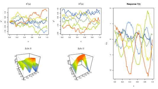
Figure 1: A sample of six realizations of the covariates and their responses jointly with the parameters for scenario 1 (Linear smooth).

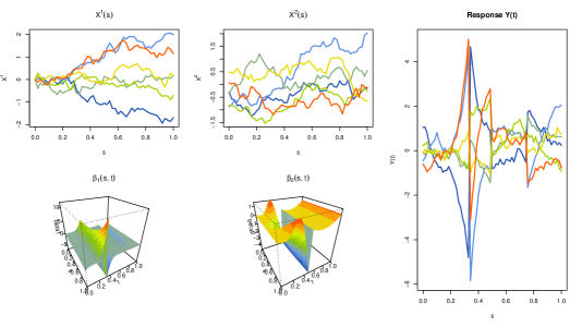
Figure 2: A sample of six realizations of the covariates and their responses jointly with the parameters for scenario 2 (Linear non–smooth).

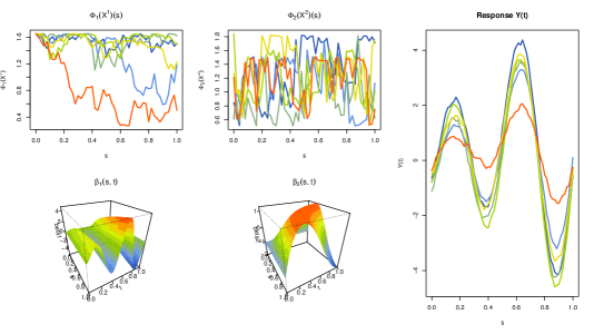
Figure 3: A sample of six realizations of the transformations of the covariates and its response jointly with the parameters for scenario 3 (Nonlinear smooth).

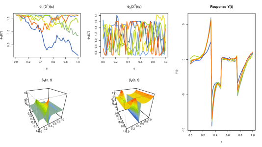
Figure 4: A sample of six realizations of the transformations of the covariates and the response jointly with the parameters for scenario 4 (Nonlinear non–smooth).

Scenarios LS (Figure 1) and NLS (Figure 3) are considered “smooth” in the sense that all the parameters and transformations involved are fairly smooth. On the other hand, scenarios LNS (Figure 2) and NLNS (Figure 4) use some parameters that are discontinuous in some null-measure subsets of their domains. It seems quite “non–smooth” for the methods based on representing all the involved functions on a smooth basis like B–splines.

			Linear smooth
$n=100$
	cov.	FLMFR	FSAMFR	FKAMFR	PFR	FAMM	LSC	DISC
$R_{e}^{2}$	1	0.818	0.857	0.848	0.811	0.866	0.805	0.806
$R_{p}^{2}$	1	0.780	0.740	0.768	0.776	0.609	0.794	0.793
$R_{e}^{2}$	2	0.818	0.856	0.843	0.812	0.865	0.808	0.808
$R_{p}^{2}$	2	0.775	0.734	0.747	0.770	0.585	0.783	0.778
$n=200$
$R_{e}^{2}$	1	0.809	0.827	0.835	0.802	0.832	0.802	0.803
$R_{p}^{2}$	1	0.793	0.781	0.781	0.788	0.746	0.800	0.799
$R_{e}^{2}$	2	0.809	0.828	0.838	0.804	0.833	0.806	0.806
$R_{p}^{2}$	2	0.784	0.769	0.761	0.779	0.739	0.787	0.783
			Linear non–smooth
$n=100$
	cov.	FLMFR	FSAMFR	FKAMFR	PFR	FAMM	LSC	DISC
$R_{e}^{2}$	1	0.811	0.842	0.847	0.237	0.345	0.707	0.703
$R_{p}^{2}$	1	0.770	0.737	0.758	0.213	0.270	0.688	0.683
$R_{e}^{2}$	2	0.810	0.839	0.844	0.348	0.436	0.732	0.726
$R_{p}^{2}$	2	0.781	0.748	0.742	0.324	0.358	0.716	0.713
$n=200$
$R_{e}^{2}$	1	0.802	0.818	0.838	0.231	0.330	0.704	0.705
$R_{p}^{2}$	1	0.775	0.761	0.763	0.219	0.295	0.689	0.687
$R_{e}^{2}$	2	0.801	0.817	0.840	0.343	0.419	0.729	0.727
$R_{p}^{2}$	2	0.790	0.780	0.764	0.331	0.394	0.723	0.720
			Nonlinear smooth
$n=100$
	cov.	FLMFR	FSAMFR	FKAMFR	PFR	FAMM	LSC	DISC
$R_{e}^{2}$	1	0.101	0.843	0.861	0.099	0.866	0.057	0.807
$R_{p}^{2}$	1	-0.112	0.741	0.730	-0.097	0.586	-0.062	0.790
$R_{e}^{2}$	2	0.100	0.820	0.840	0.099	0.853	0.054	0.779
$R_{p}^{2}$	2	-0.106	0.716	0.711	-0.094	0.559	-0.053	0.770
$n=200$
$R_{e}^{2}$	1	0.051	0.817	0.830	0.050	0.830	0.030	0.804
$R_{p}^{2}$	1	-0.049	0.764	0.749	-0.042	0.739	-0.030	0.790
$R_{e}^{2}$	2	0.054	0.794	0.819	0.053	0.815	0.030	0.778
$R_{p}^{2}$	2	-0.060	0.734	0.716	-0.052	0.710	-0.032	0.755
			Nonlinear non–smooth
$n=100$
	cov.	FLMFR	FSAMFR	FKAMFR	PFR	FAMM	LSC	DISC
$R_{e}^{2}$	1	0.101	0.830	0.856	-10.835	-10.567	-4.043	-3.398
$R_{p}^{2}$	1	-0.097	0.706	0.721	-9.949	-9.685	-3.799	-3.074
$R_{e}^{2}$	2	0.099	0.791	0.807	-9.231	-8.972	-3.429	-2.807
$R_{p}^{2}$	2	-0.102	0.621	0.628	-9.277	-9.036	-3.526	-2.878
$n=200$
$R_{e}^{2}$	1	0.052	0.800	0.827	-10.188	-7.966	-3.824	-3.147
$R_{p}^{2}$	1	-0.052	0.736	0.735	-10.416	-8.163	-3.955	-3.255
$R_{e}^{2}$	2	0.050	0.753	0.796	-9.557	-7.265	-3.572	-2.925
$R_{p}^{2}$	2	-0.045	0.676	0.667	-9.239	-7.028	-3.486	-2.838

Table 1: Simulation results ($R_{e}^{2}$ and $R_{p}^{2}$) for scenarios 1-4 with $\rho^{2}=0.80$.

Table 1 shows the results for each scenario, with two sample sizes ($n\in\{100,200\}$), $\rho^{2}=0.80$ and with one or two covariates (column cov.). The tables for all scenarios, $\rho$’s, and sample sizes are shown in the supplementary material. The rows beginning with $R^{2}_{e}$ correspond to the estimation set (each cell is the average of $n\times 100$ values) and those beginning with $R^{2}_{p}$ correspond to the prediction set (each cell is the mean of $n_{p}\times 100=10000$ values). The nearest values to the nominal value in each row are marked in bold.

The results for the Linear smooth scenario are the expected ones for all methods with a tendency to overfit for the nonlinear ones: FSAMFR, FKAMFR, and more acute for FAMM. This tendency can be detected with values over the nominal level $\rho^{2}=0.80$ in the estimation set and below this quantity in the prediction set. Also, in the Supplementary Material, the box plots for all the replicas and scenarios are plotted and this tendency can be easily checked. The choices of trivariate tensor product lengths in FAMM were splinepars=list(bs="ps", k=c(11,5,5), m=2)) using a $5$–fold CV. As one can see from Table 1, the FLMFR, PFR, LSC, and DISC models have closer values of $R_{e}^{2}$ and $R^{2}_{p}$ to the nominal level.

The results for the Linear non-smooth scenario are clearly bad for PFR and FAMM, and not so good for LSC and DISC. Recall that these methods are strongly based on representing the intermediate functions in a B–spline basis and the $\beta$ parameters of this scenario have discontinuities for certain lines (in any case, belonging to $\mathcal{L}_{2}(S)\times\mathcal{L}_{2}(T)$). An example showing the prediction of the methods for “extreme” observations (trajectories that are far from the cloud center on $\mathcal{X}^{(1)}$, $\mathcal{X}^{(2)}$, or both) are shown in the supplementary material. Although all models suffer trying to predict these extreme observations, the predictions provided by PFR and FAMM cannot capture the sharpness of the response trajectories (see Figure 11 in supplementary material). The FLMFR method that uses a PC basis is clearly the best one in this scenario although FSAMFR and FKAMFR are quite close but maintain a tendency to overfit.

In the nonlinear smooth and non-smooth scenarios, the methods FLMFR, PFR, and LSC fail as expected. The DISC method performs well for the smooth case, while for the non-smooth case, the only winners are FKAMFR and FSAMFR. The extremely negative values in the nonlinear non-smooth case are due to the smoothed predictions in the neighborhood of the discontinuities of the response from FAMM, LSC, and DISC methods (see Figure 13 in supplementary material).

6 Real Data Applications

In this section, we consider two real data applications to examine the performance of all competitor methods. A third example is available in the supplementary material.

6.1 Bike-sharing Data

To illustrate how our proposed function-on-function methods work, we use the Bike-sharing data (Fanaee-T and Gama, (2014)) as our first example. This data set is collected by Capital Bikeshare System (CBS), Washington D.C., USA. The number of casual bike rentals (NCBR) is considered as our functional response, and Temperature (T), Humidity (H), Wind Speed (WS) and Feeling Temperature (FT), are the functional covariates. These variables are recorded each hour from January 1, 2011, to December 1, 2012. Similar to Kim et al., (2018), we only consider the data for Saturday trajectories, and NBCR is log–transformed to avoid its natural heteroscedasticity. Ignoring three curves with missing values, the data set contains 102 trajectories, each with 24 data points (hourly) for all variables. The corresponding plots are displayed in Figure 5. Table 2 contains the distance correlation between all variables. It reveals that FT has the highest distance correlation with the response ($\log(\textbf{NCBR}+1)$).

Distance correlation
	NCBR	$\log(\textbf{NCBR}+1)$	T	H	WS
T	0.527	0.678
H	0.067	0.069	0.054
WS	0.062	0.102	0.057	0.053
FT	0.552	0.705	0.994	0.054	0.060

Table 2: Distance correlation among functional variables in Bike-sharing data.

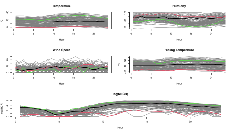
Figure 5: The plot of Bike-sharing variables over 112 Saturdays from January 1, 2011 to December 1, 2012. The black, red, and green lines correspond to dates September 17, 2011, January 21, 2012, and January 9, 2012, respectively.

Based on these values, a variable selection algorithm is performed similarly to the one proposed by Febrero-Bande et al., (2019), and the covariates FT, H, and WS were selected as relevant for the response (in that order). Note that the selection algorithm does not select T due to its collinearity/concurvity with FT (dCor:$0.994$). The observations are randomly split into train and test sets (82 observations are considered for the train set, and the remaining $20$ are allocated to the test set). We repeat this procedure 20 times and compute the $R_{p}^{2}$ for each one. Table 3 shows the results for the aforementioned methods once, including the sub-models in order of their relevance. The median of $R^{2}_{p}$ is shown instead of the mean as FAMM fails to converge in some cases (2–4 repetitions) due to numerical instabilities. Also, the number of repetitions is pretty low due to the FAMM consuming-time requirements.

$\mathcal{Y}=\log(\textbf{NCBR}+1)$
covariates	FLMFR	FSAMFR	FKAMFR	PFR	FAMM	LSC	DISC
FT	0.543	0.595	0.591	0.549	0.502	0.562	0.595
FT, H	0.565	0.599	0.640	0.568	0.445	0.563	0.652
FT, H, WS	0.554	0.563	0.638	0.555	0.529	0.533	0.662

Table 3: Median of $R^{2}_{p}$ for the methods (including the covariates in order of importance) for predicting $\log(\textbf{NCBR}+1)$. The two highest values per row are printed in bold.

Table 3 reveals that whether we include all the covariates or only a subset of them, nonlinear methods provide better prediction performance than linear methods. However, the differences between the two groups are slight. With FT, all methods achieve a certain level that is slightly modified when we add more covariates. The addition of a second covariate slightly improves the $R^{2}_{p}$ for FKAMFR and DISC but shows a decreasing term for FAMM. FLMFR, FSAMFR, PFR, and LSC show an almost constant effect with respect to the addition of covariates. The behavior of FAMM is an exception showing a V-shape along covariates. The slight improvement from two to three covariates (or even decrease) suggests that the inclusion of the third covariate (WS) adds more uncertainty to estimation than prediction power.

An important issue that deserves a detailed discussion is the computational cost. In this example, when needed, FT is represented in two PCs, H in four PCs, and WS in six PCs to ensure at least 95% of the variability of each covariate is explained. The response needs six PCs to explain 90% of the variability. These parameters are related to the complexity that can be derived from the trace of the hat matrix $H$ ($\hat{\mathcal{Y}}=H\mathcal{Y}$). For instance, in FLMFR, each covariate consumes degrees of freedom equal to the number of PCs employed. In the case of FSAMFR, the consumed degrees of freedom is $\sum_{j=1}^{nPCs}k_{j}$ where $k_{j}$ is the complexity of the function associated with the $j^{\rm th}$ PC (by default up to eight). Specifically, in this example, $k_{j}$ is limited to five to have fewer parameters than the number of data. The effect on the complexity of FAMM, LSC, and DISC due to the number of PC of the covariates is not apparent. The reason is that, internally, these methods represent the information on a B–spline basis. Therefore, it seems that the complexity is mainly related to the length of the B–spline basis plus some penalizing factors like in the linear method LSC. In the nonlinear methods, FAMM and DISC, this effect is even worse by adding parameters for the spline representation of the values that add complexity to the estimation process. This makes the choice of the parameters a crucial step but, unfortunately, the help of these packages does not provide further information. The complexity of FKAMFR is derived from the bandwidth values associated with each covariate, and it does not depend on the PC representation of the covariates. Regarding computational time, FLMFR, FSAMFR, LSC, and DISC obtain times measured in milliseconds ($51.5$, $266.2$, $112.9$, and $559.5$, respectively), with important differences among them. PFR extends to $5.47$ seconds, and FKAMFR needs $27.32$ seconds, mostly employed in computing the optimal bandwidths and on the cycles of the back-fitting algorithm. Finally, FAMM extends its time to $489.7$ seconds even with a tiny choice of the parameters (k=c(7,7,7)). Recall that the use of nonlinear contributions with command sff is considered an experimental feature by its authors.

6.2 Electricity Demand and Price Data

Another interesting example comes from the Iberian Energy Market. Specifically, the daily profiles of Electricity Price ($\textbf{Pr}_{d}$) and Demand ($\textbf{En}_{d}$) (the index refers to a day), both measured hourly, are obtained from two biannual periods separated by ten years: 2008-2009 and 2018-2019 (source:omie.es). Febrero-Bande et al., (2019) also employ this data, but they use a different period and focus on variable selection for scalar responses. Comparing the two periods, the profiles (see Figure 6) show a considerable reduction in demand but not followed by a similar reduction in price.

Figure 6: Profiles for Electricity Demand (first row) and Electricity Price (second row) for the periods 2008-09 (first column) and 2018-19 (second column). The black line corresponds to the functional mean of each data set.

In this example, a possible linear relationship among these two covariates is explored ($\textbf{Pr}_{d}$ explained by $\textbf{En}_{d}$) via a simulation study. In the simulation, we use $100$ repetitions, where each period is randomly split into a training and a prediction subset (75%-25%). All the models described above with only one covariate are applied to the training sample, and $R^{2}_{p}$ is computed from the prediction sample for impartial comparative purposes. When necessary, four principal components were employed for representing Pr and En (more than 95% of explained variability is obtained in both cases). The results of the $100$ repetitions are shown in Table 4 and Figure 7, where a significant difference between the two periods is observed. DISC and FKAMFR obtain the two best results in both cases with $0.576$ (DISC) and $0.565$ (FKAMFR) for 2008-09. The other nonlinear methods obtain $0.460$ (FAMM), and $0.424$ (FSAMFR). The linear methods have results between $0.473$ (LSC) and $0.306$ (PFR), suggesting that there is a clear nonlinear relationship among $\textbf{Pr}_{d}$ and $\textbf{En}_{d}$ perhaps due to some clusters owing to different patterns for groups of days (labor vs weekend days). The conclusions for the second period are completely different. See the box plots in Figure 7, which are drawn at the same scale. The numerical results are between $0.230$ (FKAMFR) and $0.137$ (PFR), suggesting a weak linear relationship among covariates. As in this case, we have only one covariate, we can apply the test of linearity between a single functional covariate and a functional response described by García-Portugués et al., (2021). For both periods, we obtain zero $p$-values, and thus, we reject the linear hypothesis.

$\mathcal{Y}=\textbf{Pr}_{d}\sim\textbf{En}_{d}$
$\bar{R}_{p}^{2}$	FLMFR	FSAMFR	FKAMFR	PFR	FAMM	LSC	DISC
2008-09	0.313	0.424	0.565	0.306	0.460	0.473	0.576
2018-19	0.143	0.194	0.230	0.137	0.165	0.197	0.201

Table 4: Mean of $R_{p}^{2}$ for the Energy data. Periods: 2008-09 and 2018-19.

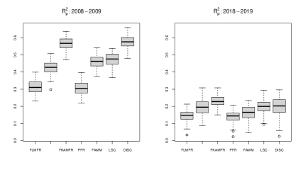
Figure 7: Boxplots for $R^{2}_{p}$ ($100$ repetitions) for two different periods: 2008-2009 (left panel) and 2018-2019 (right panel).

The relevant covariates for constructing predictive models (using information up to $d-1$ to explain $d$) selected in Febrero-Bande et al., (2019) include mainly the lagged functional covariates at $d-1$ and $d-7$. Following the same idea, we implement a numerical study ($100$ repetitions) to explain $\textbf{Pr}_{d}$ with covariates $\textbf{En}_{d-1}$, $\textbf{En}_{d-7}$ and with $\textbf{Pr}_{d-1}$, $\textbf{Pr}_{d-7}$ using only the period 2008-09. Again, we split the data into training and prediction samples (75%-25%) with $543$ curves in the training and $181$ in the prediction sample. Table 5 summarizes the results. The first row (covariates $\textbf{En}_{d-1}$, $\textbf{En}_{d-7}$) is similar to Table 4 but with a rise of about $0.1$ for FKAMFR, FAMM, LSC and DISC. The nonlinear methods show a clear gap with respect to linear methods. When the covariates are $\textbf{Pr}_{d-1}$ and $\textbf{Pr}_{d-7}$ (second row), the model seems linear because all models obtain almost the same high results (around $0.89$). This suggests that $\textbf{Pr}_{d}$ follows a persistent process, where tomorrow’s price is almost perfectly explained with today’s and the last week’s price. In any case, the gap among the rows of Table 5 suggests that there are other factors more important than the load/demand for determining the electricity prices.

Another important factor to take into account is computational time. FLMFR and FSAMFR take about three seconds, while PFR, LSC, and DISC need 10 to 18 seconds. FKAMFR and FAMM go over two minutes to complete their computations and particularly FAMM, depending on its parameters and sample size, can easily last more than 30 minutes.

$\mathcal{Y}=\textbf{Pr}_{d}$
$\bar{R}_{p}^{2}$	FLMFR	FSAMFR	FKAMFR	PFR	FAMM	LSC	DISC
$\textbf{En}_{d-1}$, $\textbf{En}_{d-7}$	0.330	0.469	0.632	0.318	0.560	0.595	0.660
$\textbf{Pr}_{d-1}$, $\textbf{Pr}_{d-7}$	0.889	0.887	0.883	0.886	0.860	0.897	0.883

Table 5: Average of $R_{p}^{2}$ for prediction models with response $\textbf{Pr}_{d}$. Period: 2008-09. The two highest values per row are printed in bold.

7 Concluding Remarks and Outlooks

In this paper, a review of functional regression models with functional response was provided jointly with two new nonlinear proposals: FSAMFR and FKAMFR. Both are extensions of functional regression models with the scalar response and the main difference between them is the nature of the functional spaces associated with the response and the covariates. As FSAMFR is based on the representation of all functional information in bases, this proposal is restricted to be applied when the response and the covariates spaces are Hilbert. On the other hand, the estimation of an FKAMFR model mimics usual kernel regression models but uses distances allowing it to be applied to general metric or normed spaces. The new proposals have been implemented in both functions that will be available in the next version of package fda.usc (the present implementation is provided in the supplementary material with the package fda.usc.devel). Also, a new implementation of a functional linear regression model (FLMFR) is provided that, contrary to previous approaches, does not need to assume that the response trajectories are smooth. The previous approaches, linear (PFR and LSC) or nonlinear (FAMM and DISC), always represent the estimates using a B–spline basis that can have difficulties in scenarios with discrete discontinuities (see, for instance, scenario 2 in the simulation study). These previous approaches are not similar with respect to their availability. The performance of the methods included in FRegSigCom (LSC and DISC) is competitive but the development of the package seems to be discontinued and only old versions can be installed. The refund package (PFR and FAMM) has a continuous development and the performance of PFR seems reasonable when the trajectories are quite smooth. On the contrary, in our simulation scenarios, the application of FAMM, particularly with several functional covariates, was unable to obtain similar results to the other methods even though several combinations of the parameters have been tried.

As a future work, one can extend FRMFR to estimate functional time series with functional responses using a similar framework. Note that treating a functional time series as an FRMFR requires adding additional assumptions to parameters and covariates, such as stationarity, and introducing new tools for testing or capturing the temporal characteristics of the functional time series.

Supplementary Material

A Visualization Tool about Linear-Nonlinear Relationships

In a multivariate framework, it could be relatively easy to construct some diagnostic plots for assessing when the partial contribution of a covariate is linear or nonlinear. This is extremely difficult in FDA due to the high dimensionality of objects involved. Nevertheless, something can be done in the case of Hilbertian response and a single Hilbertian covariate as shown in Figures 8 and 9. In both cases, we have a matrix of plots $7\times 3$ where the columns correspond with the $j^{\rm th}$ PC of the response ($Y.PC_{j}$). The rows are associated with the models described in the paper. And, in each row-column combination, a map of the predicted score for the $j^{\rm th}$ of the response is plotted for a grid of predictor $\mathcal{X}_{0}=\mu_{\mathcal{X}}+x_{0,1}\eta_{1}+x_{0,2}\eta_{2}$, where $x_{0,1}$ and $x_{0,2}$ are generated in the range of the training sample and $\eta_{1}$, $\eta_{2}$, are the first two principal components of the covariate. All the plots have the same scale by columns in order to compare the different models. Also, the dotted line inside each map is the convex hull of $x_{i,1}$ and $x_{i,2}$ from the training sample. The comparison among models must be done inside this polygon although the data cloud is not uniformly filling that convex hull.

Figure 8 corresponds to a linear example and the maps for all models are more or less the same except perhaps for FAMM (row 5) where a different pattern is shown (it seems smoother than the others in the first PC). The map for the first PC shows a clear decreasing trend from top to bottom that is also captured by the nonlinear methods (FSAMFR, FKAMFR, and DISC). For the second PC, FSAMFR and FKAMFR provide a nonlinear pattern that seems not so different from the linear models inside the convex hull polygon.

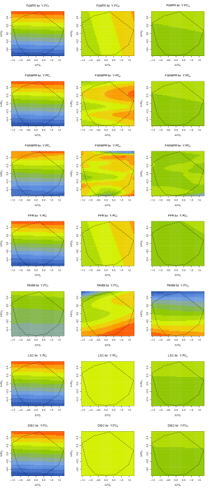
Figure 8: Maps for predictive response PC scores (by columns) as a function of the first two PC of the single covariate (Linear example). The dotted polygon inside each plot is the convex hull of the first two PCs of the covariate.

Figure 9 shows an example of a nonlinear model that, as expected, is captured by FSAMFR, FKAMFR, and DISC principally in the first PC (first column). FAMM captures a smoother version of the first PC and has a different pattern to the second and third PC (possibly to compensate for its estimation of the first PC). The linear models (FLMFR, PFR, and LSC) show a similar pattern among them different from the pattern captured by the nonlinear models.

For several covariates, a similar tool can be done by fixing other covariates to particular values such as their mean and creating predictor vectors in the same way as before generating a grid using the two first PC components. But, it may happen that the plot seems linear because the non-linearity was located far from the chosen fixed point. So, when this visualization tool shows a partial linear relationship, it is not a complete warranty about that assumption.

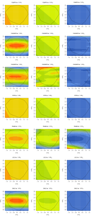
Figure 9: Maps for predictive response PC scores (by columns) as a function of the first two PC of the single covariate (Nonlinear example). The dotted polygon inside each plot is the convex hull of the first two PCs of the covariate.

Detailed results of the numerical study and in–depth analysis of a single replica.

Figures 10–13 show examples of just one replica for scenarios 1–4 focusing on the prediction of “extreme” observations defined as those observations with trajectories for $\mathcal{X}_{1}$, $\mathcal{X}_{2}$ or both far from the center of the trajectories. The first row of the figures shows the extreme observations that are predicted in the second row by all methods. Each figure of the second row shows the true trajectories (thick lines) that are predicted. The first figure of the second row shows the predictions of FLMFR (thin lines), FSAMFR (dashed lines), and FKAMFR (dotted lines). The second figure contains the predictions of PFR (thin lines) and FAMM (dashed lines). And third, shows the predictions of LSC (thin lines) and DISC (dashed lines). The thin lines correspond with the prediction of linear methods whereas the dashed/dotted lines are predictions from nonlinear ones. Predictions and true trajectories are paired by colors. From these figures, some clues can be extracted about the performance of the methods. For instance, in Figure 10 the black curve is extreme mostly because $\mathcal{X}_{1}$ is far from the center and the red and green ones are extreme by $\mathcal{X}_{2}$. All the methods except FAMM provide reasonable predictions for the black curve. The red and green predictions are not so close to the true trajectories for all models but again, FAMM obtain a worse result. In scenario 2 (Figure 11) the main reason for the bad prediction for PFR and FAMM comes from the lack of these methods to adapt the peaks of the response. In scenario 3 (Figure 12), the linear methods are not able to be close to the true curves in the bumps. Finally, in scenario 4 (Figure 13), PFR, FAMM, LSC, and DISC fail due to their smooth representation of the response. FLMFR mainly fails the prediction around point $0.35$.

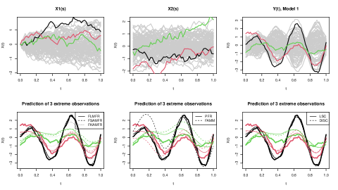
Figure 10: Prediction of 3 extreme observations. The first row shows the trajectories for $\mathcal{X}_{1}$, $\mathcal{X}_{2}$, and $\mathcal{Y}$ with respect to the training set (in gray). The predictions are shown in the second row.

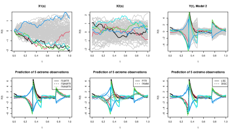
Figure 11: Prediction of 5 extreme observations. The first row shows the trajectories for $\mathcal{X}_{1}$, $\mathcal{X}_{2}$, and $\mathcal{Y}$ with respect to the training set (in gray). The predictions are shown in the second row.

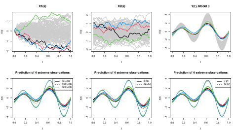
Figure 12: Prediction of 4 extreme observations. The first row shows the trajectories for $\mathcal{X}_{1}$, $\mathcal{X}_{2}$, and $\mathcal{Y}$ with respect to the training set (in gray). The predictions are shown in the second row.

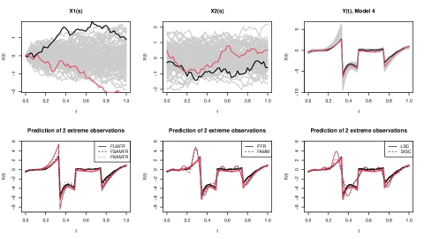
Figure 13: Prediction of 2 extreme observations. The first row shows the trajectories for $\mathcal{X}_{1}$, $\mathcal{X}_{2}$, and $\mathcal{Y}$ with respect to the training set (in gray). The predictions are shown in the second row.

The complete tables derived from the numerical study are shown in the following. Tables 6–7 show the results for $\rho^{2}=0.65$ for scenarios 1–4. Tables 8–9 show the results for $\rho^{2}=0.80$ and the same is shown in Tables 10–11 for $\rho^{2}=0.90$. There is a clear tendency to overfitting in most of the nonlinear methods in linear scenarios. This is more acute for $N=50$ and especially for FAMM which seems very affected by small sizes. The negative results in the prediction rows correspond with scenarios where the model is not able to produce good predictions of new data because the model cannot explain the example (linear model vs nonlinear example) or the size for estimation is too small.

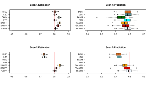
Figure 14: Boxplots of the replicas for scenarios 1–2, $\rho^{2}=0.8$ and $N=200$ for all models.

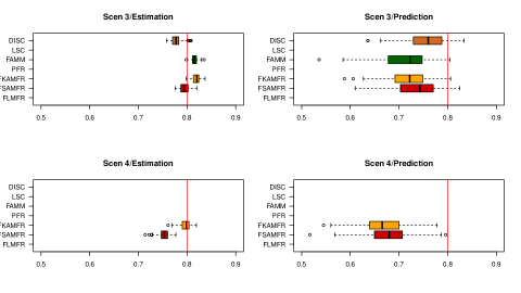
Figure 15: Boxplot of the replicas for scenarios 3–4, $\rho^{2}=0.8$ and $N=200$ for all models.

The box-plots shown in Figures 14 and 15 correspond with the replicas ($R^{2}_{e}$ and $R^{2}_{p}$) for the four scenarios with $\rho^{2}=0.80$ and $N=200$. The boxes that are out of the interval $[0.5,0.9]$ are not shown.

			Linear smooth
$n=50$
	cov.	FLMFR	FSAMFR	FKAMFR	PFR	FAMM	LSC	DISC
$R_{e}^{2}$	1	0.711	0.786	0.730	0.703	0.895	0.665	0.665
$R_{p}^{2}$	1	0.586	0.486	0.596	0.586	-5.369	0.636	0.633
$R_{e}^{2}$	2	0.712	0.787	0.721	0.704	0.893	0.672	0.666
$R_{p}^{2}$	2	0.589	0.487	0.577	0.588	-5.887	0.622	0.615
$n=100$
	cov.	FLMFR	FSAMFR	FKAMFR	PFR	FAMM	LSC	DISC
$R_{e}^{2}$	1	0.682	0.747	0.716	0.676	0.767	0.659	0.659
$R_{p}^{2}$	1	0.627	0.557	0.621	0.624	0.313	0.649	0.648
$R_{e}^{2}$	2	0.681	0.742	0.712	0.675	0.767	0.664	0.660
$R_{p}^{2}$	2	0.619	0.557	0.599	0.617	0.274	0.632	0.626
$n=200$
$R_{e}^{2}$	1	0.666	0.697	0.698	0.660	0.706	0.654	0.654
$R_{p}^{2}$	1	0.635	0.610	0.627	0.631	0.552	0.646	0.646
$R_{e}^{2}$	2	0.664	0.697	0.702	0.660	0.706	0.657	0.654
$R_{p}^{2}$	2	0.638	0.615	0.616	0.634	0.559	0.643	0.639
			Linear non–smooth
$n=50$
	cov.	FLMFR	FSAMFR	FKAMFR	PFR	FAMM	LSC	DISC
$R_{e}^{2}$	1	0.699	0.759	0.724	0.224	0.418	0.577	0.575
$R_{p}^{2}$	1	0.585	0.501	0.590	0.135	-0.864	0.548	0.548
$R_{e}^{2}$	2	0.697	0.755	0.722	0.320	0.515	0.609	0.605
$R_{p}^{2}$	2	0.592	0.518	0.553	0.220	-0.977	0.560	0.564
$n=100$
	cov.	FLMFR	FSAMFR	FKAMFR	PFR	FAMM	LSC	DISC
$R_{e}^{2}$	1	0.671	0.729	0.713	0.205	0.336	0.576	0.568
$R_{p}^{2}$	1	0.611	0.548	0.604	0.160	0.080	0.551	0.551
$R_{e}^{2}$	2	0.669	0.722	0.715	0.296	0.418	0.600	0.592
$R_{p}^{2}$	2	0.623	0.573	0.592	0.247	0.140	0.576	0.576
$n=200$
$R_{e}^{2}$	1	0.658	0.687	0.702	0.196	0.297	0.576	0.569
$R_{p}^{2}$	1	0.635	0.615	0.627	0.173	0.210	0.567	0.563
$R_{e}^{2}$	2	0.656	0.681	0.707	0.284	0.370	0.595	0.589
$R_{p}^{2}$	2	0.630	0.610	0.607	0.258	0.267	0.580	0.577

Table 6: Simulation results ($R_{e}^{2}$ and $R_{p}^{2}$) for scenarios 1–4 with $\rho^{2}=0.65$.

			Nonlinear smooth
$n=50$
	cov.	FLMFR	FSAMFR	FKAMFR	PFR	FAMM	LSC	DISC
$R_{e}^{2}$	1	0.178	0.758	0.762	0.179	0.893	0.075	0.671
$R_{p}^{2}$	1	-0.221	0.482	0.537	-0.204	-5.940	-0.093	0.620
$R_{e}^{2}$	2	0.188	0.746	0.741	0.190	0.891	0.101	0.647
$R_{p}^{2}$	2	-0.207	0.467	0.524	-0.191	-6.950	-0.114	0.614
$n=100$
	cov.	FLMFR	FSAMFR	FKAMFR	PFR	FAMM	LSC	DISC
$R_{e}^{2}$	1	0.093	0.727	0.742	0.093	0.767	0.044	0.662
$R_{p}^{2}$	1	-0.104	0.556	0.585	-0.094	0.299	-0.053	0.636
$R_{e}^{2}$	2	0.097	0.716	0.728	0.097	0.758	0.046	0.640
$R_{p}^{2}$	2	-0.112	0.529	0.562	-0.102	0.240	-0.060	0.616
$n=200$
$R_{e}^{2}$	1	0.046	0.683	0.720	0.046	0.705	0.022	0.655
$R_{p}^{2}$	1	-0.048	0.613	0.606	-0.043	0.559	-0.026	0.647
$R_{e}^{2}$	2	0.048	0.666	0.707	0.048	0.693	0.024	0.633
$R_{p}^{2}$	2	-0.051	0.575	0.571	-0.047	0.525	-0.026	0.608
			Nonlinear non–smooth
$n=50$
	cov.	FLMFR	FSAMFR	FKAMFR	PFR	FAMM	LSC	DISC
$R_{e}^{2}$	1	0.178	0.757	0.759	-8.944	-8.804	-3.318	-2.815
$R_{p}^{2}$	1	-0.194	0.449	0.534	-8.117	-7.995	-3.122	-2.519
$R_{e}^{2}$	2	0.189	0.727	0.692	-7.894	-7.752	-2.906	-2.445
$R_{p}^{2}$	2	-0.218	0.371	0.442	-7.429	-7.314	-2.857	-2.330
$n=100$
	cov.	FLMFR	FSAMFR	FKAMFR	PFR	FAMM	LSC	DISC
$R_{e}^{2}$	1	0.097	0.720	0.747	-8.516	-8.292	-3.183	-2.660
$R_{p}^{2}$	1	-0.097	0.522	0.568	-8.324	-8.114	-3.172	-2.594
$R_{e}^{2}$	2	0.096	0.688	0.692	-7.810	-7.593	-2.901	-2.404
$R_{p}^{2}$	2	-0.101	0.455	0.495	-7.584	-7.392	-2.885	-2.365
$n=200$
$R_{e}^{2}$	1	0.049	0.671	0.718	-8.418	-6.584	-3.159	-2.620
$R_{p}^{2}$	1	-0.047	0.572	0.585	-8.572	-6.725	-3.252	-2.694
$R_{e}^{2}$	2	0.046	0.632	0.685	-7.719	-5.861	-2.886	-2.366
$R_{p}^{2}$	2	-0.043	0.525	0.522	-7.767	-5.923	-2.933	-2.421

Table 7: Simulation results ($R_{e}^{2}$ and $R_{p}^{2}$) for scenarios 1–4 with $\rho^{2}=0.65$.

			Linear smooth
$n=50$
	cov.	FLMFR	FSAMFR	FKAMFR	PFR	FAMM	LSC	DISC
$R_{e}^{2}$	1	0.837	0.875	0.855	0.829	0.940	0.811	0.812
$R_{p}^{2}$	1	0.758	0.705	0.750	0.754	-2.716	0.790	0.786
$R_{e}^{2}$	2	0.834	0.877	0.844	0.827	0.939	0.814	0.810
$R_{p}^{2}$	2	0.766	0.708	0.726	0.761	-3.690	0.782	0.776
$n=100$
	cov.	FLMFR	FSAMFR	FKAMFR	PFR	FAMM	LSC	DISC
$R_{e}^{2}$	1	0.818	0.857	0.848	0.811	0.866	0.805	0.806
$R_{p}^{2}$	1	0.780	0.740	0.768	0.776	0.609	0.794	0.793
$R_{e}^{2}$	2	0.818	0.856	0.843	0.812	0.865	0.808	0.808
$R_{p}^{2}$	2	0.775	0.734	0.747	0.770	0.585	0.783	0.778
$n=200$
$R_{e}^{2}$	1	0.809	0.827	0.835	0.802	0.832	0.802	0.803
$R_{p}^{2}$	1	0.793	0.781	0.781	0.788	0.746	0.800	0.799
$R_{e}^{2}$	2	0.809	0.828	0.838	0.804	0.833	0.806	0.806
$R_{p}^{2}$	2	0.784	0.769	0.761	0.779	0.739	0.787	0.783
			Linear non–smooth
$n=50$
	cov.	FLMFR	FSAMFR	FKAMFR	PFR	FAMM	LSC	DISC
$R_{e}^{2}$	1	0.826	0.863	0.853	0.244	0.373	0.707	0.702
$R_{p}^{2}$	1	0.758	0.706	0.740	0.204	0.158	0.683	0.681
$R_{e}^{2}$	2	0.826	0.860	0.843	0.360	0.469	0.737	0.733
$R_{p}^{2}$	2	0.757	0.711	0.706	0.301	0.265	0.703	0.699
$n=100$
	cov.	FLMFR	FSAMFR	FKAMFR	PFR	FAMM	LSC	DISC
$R_{e}^{2}$	1	0.811	0.842	0.847	0.237	0.345	0.707	0.703
$R_{p}^{2}$	1	0.770	0.737	0.758	0.213	0.270	0.688	0.683
$R_{e}^{2}$	2	0.810	0.839	0.844	0.348	0.436	0.732	0.726
$R_{p}^{2}$	2	0.781	0.748	0.742	0.324	0.358	0.716	0.713
$n=200$
$R_{e}^{2}$	1	0.802	0.818	0.838	0.231	0.330	0.704	0.705
$R_{p}^{2}$	1	0.775	0.761	0.763	0.219	0.295	0.689	0.687
$R_{e}^{2}$	2	0.801	0.817	0.840	0.343	0.419	0.729	0.727
$R_{p}^{2}$	2	0.790	0.780	0.764	0.331	0.394	0.723	0.720

Table 8: Simulation results ($R_{e}^{2}$ and $R_{p}^{2}$) for scenarios 1–4 with $\rho^{2}=0.8$.

			Nonlinear smooth
$n=50$
	cov.	FLMFR	FSAMFR	FKAMFR	PFR	FAMM	LSC	DISC
$R_{e}^{2}$	1	0.201	0.863	0.874	0.196	0.940	0.119	0.814
$R_{p}^{2}$	1	-0.248	0.707	0.693	-0.223	-3.319	-0.158	0.792
$R_{e}^{2}$	2	0.211	0.846	0.851	0.208	0.938	0.114	0.785
$R_{p}^{2}$	2	-0.220	0.664	0.668	-0.199	-2.763	-0.115	0.754
$n=100$
	cov.	FLMFR	FSAMFR	FKAMFR	PFR	FAMM	LSC	DISC
$R_{e}^{2}$	1	0.101	0.843	0.861	0.099	0.866	0.057	0.807
$R_{p}^{2}$	1	-0.112	0.741	0.730	-0.097	0.586	-0.062	0.790
$R_{e}^{2}$	2	0.100	0.820	0.840	0.099	0.853	0.054	0.779
$R_{p}^{2}$	2	-0.106	0.716	0.711	-0.094	0.559	-0.053	0.770
$n=200$
$R_{e}^{2}$	1	0.051	0.817	0.830	0.050	0.830	0.030	0.804
$R_{p}^{2}$	1	-0.049	0.764	0.749	-0.042	0.739	-0.030	0.790
$R_{e}^{2}$	2	0.054	0.794	0.819	0.053	0.815	0.030	0.778
$R_{p}^{2}$	2	-0.060	0.734	0.716	-0.052	0.710	-0.032	0.755
			Nonlinear non–smooth
$n=50$
	cov.	FLMFR	FSAMFR	FKAMFR	PFR	FAMM	LSC	DISC
$R_{e}^{2}$	1	0.203	0.850	0.875	-11.631	-11.491	-4.302	-3.705
$R_{p}^{2}$	1	-0.209	0.678	0.680	-9.983	-9.845	-3.856	-3.085
$R_{e}^{2}$	2	0.196	0.812	0.806	-9.630	-9.487	-3.536	-2.967
$R_{p}^{2}$	2	-0.222	0.568	0.571	-9.091	-8.968	-3.514	-2.833
$n=100$
	cov.	FLMFR	FSAMFR	FKAMFR	PFR	FAMM	LSC	DISC
$R_{e}^{2}$	1	0.101	0.830	0.856	-10.835	-10.567	-4.043	-3.398
$R_{p}^{2}$	1	-0.097	0.706	0.721	-9.949	-9.685	-3.799	-3.074
$R_{e}^{2}$	2	0.099	0.791	0.807	-9.231	-8.972	-3.429	-2.807
$R_{p}^{2}$	2	-0.102	0.621	0.628	-9.277	-9.036	-3.526	-2.878
$n=200$
$R_{e}^{2}$	1	0.052	0.800	0.827	-10.188	-7.966	-3.824	-3.147
$R_{p}^{2}$	1	-0.052	0.736	0.735	-10.416	-8.163	-3.955	-3.255
$R_{e}^{2}$	2	0.050	0.753	0.796	-9.557	-7.265	-3.572	-2.925
$R_{p}^{2}$	2	-0.045	0.676	0.667	-9.239	-7.028	-3.486	-2.838

Table 9: Simulation results ($R_{e}^{2}$ and $R_{p}^{2}$) for scenarios 1–4 with $\rho^{2}=0.8$.

			Linear smooth
$n=50$
	cov.	FLMFR	FSAMFR	FKAMFR	PFR	FAMM	LSC	DISC
$R_{e}^{2}$	1	0.918	0.939	0.934	0.910	0.969	0.906	0.906
$R_{p}^{2}$	1	0.879	0.848	0.858	0.873	-2.106	0.893	0.892
$R_{e}^{2}$	2	0.918	0.940	0.924	0.911	0.970	0.910	0.908
$R_{p}^{2}$	2	0.878	0.846	0.833	0.872	-0.997	0.886	0.880
$n=100$
	cov.	FLMFR	FSAMFR	FKAMFR	PFR	FAMM	LSC	DISC
$R_{e}^{2}$	1	0.908	0.928	0.930	0.901	0.933	0.902	0.903
$R_{p}^{2}$	1	0.892	0.871	0.875	0.886	0.805	0.899	0.898
$R_{e}^{2}$	2	0.909	0.928	0.923	0.902	0.933	0.905	0.905
$R_{p}^{2}$	2	0.891	0.872	0.857	0.885	0.800	0.894	0.890
$n=200$
$R_{e}^{2}$	1	0.904	0.913	0.919	0.897	0.916	0.901	0.902
$R_{p}^{2}$	1	0.895	0.889	0.882	0.889	0.875	0.898	0.898
$R_{e}^{2}$	2	0.904	0.913	0.921	0.898	0.916	0.903	0.904
$R_{p}^{2}$	2	0.894	0.888	0.870	0.888	0.872	0.895	0.892
			Linear non–smooth
$n=50$
	cov.	FLMFR	FSAMFR	FKAMFR	PFR	FAMM	LSC	DISC
$R_{e}^{2}$	1	0.914	0.932	0.935	0.258	0.366	0.794	0.790
$R_{p}^{2}$	1	0.888	0.862	0.858	0.256	0.340	0.790	0.784
$R_{e}^{2}$	2	0.911	0.927	0.919	0.389	0.469	0.824	0.819
$R_{p}^{2}$	2	0.875	0.853	0.811	0.356	0.434	0.801	0.796
$n=100$
	cov.	FLMFR	FSAMFR	FKAMFR	PFR	FAMM	LSC	DISC
$R_{e}^{2}$	1	0.905	0.920	0.929	0.257	0.361	0.792	0.792
$R_{p}^{2}$	1	0.887	0.870	0.866	0.251	0.348	0.785	0.783
$R_{e}^{2}$	2	0.902	0.917	0.923	0.381	0.459	0.819	0.817
$R_{p}^{2}$	2	0.886	0.872	0.844	0.373	0.450	0.810	0.807
$n=200$
$R_{e}^{2}$	1	0.901	0.909	0.916	0.256	0.359	0.791	0.791
$R_{p}^{2}$	1	0.892	0.887	0.876	0.255	0.354	0.787	0.787
$R_{e}^{2}$	2	0.898	0.905	0.923	0.379	0.456	0.818	0.816
$R_{p}^{2}$	2	0.891	0.886	0.864	0.377	0.453	0.814	0.811

Table 10: Simulation results ($R_{e}^{2}$ and $R_{p}^{2}$) for scenarios 1–4 with $\rho^{2}=0.90$.

			Nonlinear smooth
$n=50$
	cov.	FLMFR	FSAMFR	FKAMFR	PFR	FAMM	LSC	DISC
$R_{e}^{2}$	1	0.199	0.928	0.937	0.193	0.970	0.129	0.908
$R_{p}^{2}$	1	-0.246	0.845	0.799	-0.216	-0.889	-0.158	0.893
$R_{e}^{2}$	2	0.215	0.912	0.917	0.210	0.965	0.130	0.878
$R_{p}^{2}$	2	-0.233	0.787	0.752	-0.212	-1.417	-0.138	0.844
$n=100$
	cov.	FLMFR	FSAMFR	FKAMFR	PFR	FAMM	LSC	DISC
$R_{e}^{2}$	1	0.100	0.919	0.920	0.096	0.933	0.060	0.904
$R_{p}^{2}$	1	-0.107	0.860	0.829	-0.090	0.770	-0.056	0.893
$R_{e}^{2}$	2	0.104	0.896	0.903	0.101	0.918	0.058	0.875
$R_{p}^{2}$	2	-0.112	0.821	0.797	-0.098	0.747	-0.064	0.858
$n=200$
$R_{e}^{2}$	1	0.052	0.906	0.903	0.050	0.915	0.029	0.902
$R_{p}^{2}$	1	-0.051	0.876	0.851	-0.043	0.868	-0.028	0.897
$R_{e}^{2}$	2	0.055	0.883	0.890	0.054	0.897	0.033	0.879
$R_{p}^{2}$	2	-0.059	0.841	0.818	-0.051	0.835	-0.035	0.859
			Nonlinear non–smooth
$n=50$
	cov.	FLMFR	FSAMFR	FKAMFR	PFR	FAMM	LSC	DISC
$R_{e}^{2}$	1	0.228	0.919	0.937	-12.404	-12.249	-4.572	-3.904
$R_{p}^{2}$	1	-0.275	0.796	0.776	-11.659	-11.503	-4.536	-3.638
$R_{e}^{2}$	2	0.216	0.875	0.872	-11.281	-11.134	-4.131	-3.496
$R_{p}^{2}$	2	-0.261	0.688	0.662	-10.321	-10.186	-4.015	-3.205
$n=100$
	cov.	FLMFR	FSAMFR	FKAMFR	PFR	FAMM	LSC	DISC
$R_{e}^{2}$	1	0.109	0.907	0.917	-12.017	-11.715	-4.480	-3.749
$R_{p}^{2}$	1	-0.126	0.814	0.816	-11.914	-11.617	-4.568	-3.727
$R_{e}^{2}$	2	0.103	0.859	0.879	-10.805	-10.518	-4.019	-3.304
$R_{p}^{2}$	2	-0.109	0.742	0.723	-10.468	-10.194	-3.977	-3.230
$n=200$
$R_{e}^{2}$	1	0.056	0.888	0.897	-11.624	-9.098	-4.361	-3.597
$R_{p}^{2}$	1	-0.063	0.845	0.835	-11.588	-9.073	-4.403	-3.594
$R_{e}^{2}$	2	0.050	0.836	0.865	-10.248	-7.776	-3.830	-3.100
$R_{p}^{2}$	2	-0.050	0.776	0.759	-10.206	-7.752	-3.857	-3.110

Table 11: Simulation results ($R_{e}^{2}$ and $R_{p}^{2}$) for scenarios 1–4 with $\rho^{2}=0.90$.

Air Quality Data

Our last example is the Air Quality dataset (AQI) available from the UCI machine learning repository (Qi and Luo, (2019)). AQI is a popular dataset consisting of five metal oxide chemical sensors embedded into an air-quality multisensor device. The column names in the dataset begin with PT. The sensors are labeled with Carbon monoxide (CO), Non-methane hydrocarbons (NMHC), total Nitrogen Oxides (NOx), Ozone (O3) because it is supposed that its measures are related with the respective pollutants. The goal of this study is to predict the content of Benzene (C6H6) obtained through an independent analyzer considered the Ground Truth. The multisensor device is placed at a road level in an Italian city during the whole year. These sensors were collected as 24 hourly averaged concentration values each day jointly with the relative humidity (rH) as an external factor.

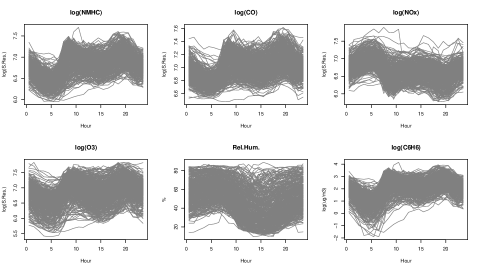
Figure 16: 355 curves for NMHC, CO, NOx, O3 (obtained from sensors), and relative humidity jointly with the response C6H6. The signals from sensors are log–transformed.

After removing the curves with missing values, we have $355$ curves for each of the six functional variables shown in Figure 16. Table 12 presents the distance correlation between functional variables in the AQI dataset. We consider the curves of $\mathcal{Y}=\ln(\textbf{C6H6})$ as the functional response and the other five variables ($\mathcal{X}_{1}=\ln(\textbf{NMHC})$, $\mathcal{X}_{2}=\ln(\textbf{O3})$, $\mathcal{X}_{3}=\ln(\textbf{CO})$, $\mathcal{X}_{4}=\ln(\textbf{NOx})$ and $\mathcal{X}_{5}=\textbf{rH}$) as the functional predictors.

Distance correlation
	$\ln(\textbf{C6H6})$	$\ln(\textbf{NMHC})$	$\ln(\textbf{CO})$	$\ln(\textbf{NOx})$	$\ln(\textbf{O3})$
$\ln(\textbf{NMHC})$	0.986
$\ln(\textbf{CO})$	0.652	0.679
$\ln(\textbf{NOx})$	0.572	0.575	0.571
$\ln(\textbf{O3})$	0.791	0.800	0.782	0.683
rH	0.069	0.071	0.219	0.195	0.169

Table 12: Distance correlation between functional variables in the AQI data.

To evaluate the performance of our proposed methods we randomly select 284 of the total observations as the training set and the rest of 71 as the test set. This procedure is repeated 100 times for the AQI data set, and after fitting each method on the training set, we estimate the regarding parameters for each method and then obtain the functional $R_{p}^{2}$ for each test set. The averages of $R_{p}^{2}$ for the $100$ repetitions are tabulated in Table 13. In this table, sets M1, M2, and M3 consider different predictors. For M1, we select only one predictor, $\ln(\textbf{NMHC})$. For M2, we select three predictors: $\ln(\textbf{NMHC})$, $\ln(\textbf{O3})$, and $\ln(\textbf{CO})$. For M3, we use all the five predictors (namely, $\ln(\textbf{NMHC})$, $\ln(\textbf{O3})$, $\ln(\textbf{CO})$, $\ln(\textbf{NOx})$, and rH). Note that we select the variables in sets M1 and M2 using a similar procedure to Febrero-Bande et al., (2019).

The results of Table 13 reveal that the performance of linear methods is roughly the same as the nonlinear methods on all three sets (M1, M2, M3). FAMM is not included in the comparison due to its high computational cost particularly when more than one predictor is used. The simulation also shows that for the inherently linear models, the performance of linear and nonlinear methods is almost the same. Thus, it seems that the function-on-function model follows a linear behavior between response and covariates on AQI. In Table 13, the results of the LSC method have always shown the highest performance. With a slight difference, DISC and FSAMFR methods have the second and third-best performances. Moreover, Table 13 reveals that the mentioned variable selection algorithm works well with this dataset. The reason is that in all six methods, increasing the number of model predictors does not improve the performance considerably.

$\mathcal{Y}=\ln(\textbf{C6H6})$
Model	FLMFR	FSAMFR	FKAMFR	PFR	LSC	DISC
M1	0.890	0.900	0.849	0.857	0.924	0.921
M2	0.893	0.902	0.858	0.864	0.927	0.912
M3	0.893	0.901	0.861	0.865	0.926	0.902

Table 13: Average of $R^{2}_{p}$ over 100 repetitions for the models (including the covariates in order of importance) for predicting $\ln(\textbf{C6H6})$. M1=$\{\mathcal{X}_{1}\}$, M2=$\{\mathcal{X}_{1},\mathcal{X}_{2},\mathcal{X}_{3}\}$, and M3=$\{\mathcal{X}_{1},\mathcal{X}_{2},\mathcal{X}_{3},\mathcal{X}_{4},\mathcal{X}_{5}\}.$

Supplementary Codes and Data

The codes and data used in this paper are available in the GitHub repository https://github.com/moviedo5/FRMFR/. From the pkg folder, the packages fda.usc.devel (devel version of fda.usc) and FRegSigCom can be installed. The latter is not currently maintained and the file .tar.gz it is a copy of its latest version published in 2018 (also available in https://cran.r-project.org/src/contrib/Archive/FRegSigCom/). The package refund can be installed from CRAN. The SimulationStudy folder contains the code that runs the whole simulation study. The RealDataApplications folder contains three files that correspond with the two examples shown in section 6 (BikeSharing2.R and omie2008vs2018.R) and the third example only shown in Supplementary Material (AirQuality.R). The datasets BikeSharing and AirQuality are included in fda.usc.devel package and are accessible through data command. The Price–Energy datasets are accessible through omel2008-09.rda and omel2018-19.rda files in the GitHub repository.

References

- Aneiros-Pérez and Vieu, (2006) Aneiros-Pérez, G. and Vieu, P. (2006). Semi-functional partial linear regression. Stat. Probabil. Lett., 76(11):1102–1110.
- Beyaztas and Shang, (2020) Beyaztas, U. and Shang, H. L. (2020). On function-on-function regression: partial least squares approach. Environ. Ecol. Stat., 27(1):95–114.
- Cardot et al., (1999) Cardot, H., Ferraty, F., and Sarda, P. (1999). Functional linear model. Stat. Probabil. Lett., 45(1):11–22.
- Cardot et al., (2003) Cardot, H., Ferraty, F., and Sarda, P. (2003). Spline estimators for the functional linear model. Stat. Sinica, 13(3):571–592.
- Cardot et al., (2007) Cardot, H., Mas, A., and Sarda, P. (2007). CLT in functional linear regression models. Probab. Theory Related Fields, 138(3):325–361.
- Chen et al., (2011) Chen, D., Hall, P., and Müller, H. (2011). Single and multiple index functional regression models with nonparametric link. Ann. Stat., 39(3):1720–1747.
- Chiou et al., (2003) Chiou, J.-M., Müller, H.-G., and Wang, J.-L. (2003). Functional quasi-likelihood regression models with smooth random effects. J. R. Stat. Soc. B, 65(2):405–423.
- Chiou et al., (2016) Chiou, J.-M., Yang, Y.-F., and Chen, Y.-T. (2016). Multivariate functional linear regression and prediction. J. Multivariate Anal., 146:301–312.
- Cuevas et al., (2002) Cuevas, A., Febrero, M., and Fraiman, R. (2002). Linear functional regression: the case of fixed design and functional response. Canad. J. Statist., 30(2):285–300.
- Delaigle et al., (2012) Delaigle, A., Hall, P., et al. (2012). Methodology and theory for partial least squares applied to functional data. Ann. Stat., 40(1):322–352.
- Fan and James, (2011) Fan, Y. and James, G. (2011). Functional additive regression. Technical report, Marshall School of Business, University of Southern California.
- Fanaee-T and Gama, (2014) Fanaee-T, H. and Gama, J. (2014). Event labeling combining ensemble detectors and background knowledge. Prog. Artif. Intell., 2(2):113–127.
- Febrero-Bande et al., (2017) Febrero-Bande, M., Galeano, P., and González-Manteiga, W. (2017). Functional principal component regression and functional partial least-squares regression: An overview and a comparative study. Int. Stat. Rev., 85(1):61–83.
- Febrero-Bande and González-Manteiga, (2013) Febrero-Bande, M. and González-Manteiga, W. (2013). Generalized additive models for functional data. TEST, 22(2):278–292.
- Febrero-Bande et al., (2019) Febrero-Bande, M., González-Manteiga, W., and de la Fuente, M. O. (2019). Variable selection in functional additive regression models. Comput. Statist., 34(2):469–487.
- Ferraty et al., (2013) Ferraty, F., Goia, A., Salinelli, E., and Vieu, P. (2013). Functional projection pursuit regression. TEST, 22(2):293–320.
- (17) Ferraty, F., González-Manteiga, W., Martínez-Calvo, A., and Vieu, P. (2012a). Presmoothing in functional linear regression. Stat. Sinica, 22(1):69–94.
- (18) Ferraty, F., Keilegom, I. V., and Vieu, P. (2012b). Regression when both response and predictor are functions. J. Multivariate Anal., 109:10–28.
- Ferraty and Vieu, (2006) Ferraty, F. and Vieu, P. (2006). Nonparametric functional data analysis: theory and practice. Springer.
- Ferraty and Vieu, (2009) Ferraty, F. and Vieu, P. (2009). Additive prediction and boosting for functional data. Comput. Stat. Data Anal., 53(4):1400–1413.
- García-Portugués et al., (2021) García-Portugués, E., Álvarez Liébana, J., Álvarez Pérez, G., and González-Manteiga, W. (2021). A goodness-of-fit test for the functional linear model with functional response. Scand. J. Stat., 48(2):502–528.
- Goldsmith et al., (2011) Goldsmith, J., Bobb, J., Crainiceanu, C.-M., Caffo, B., and Reich, D. (2011). Penalized functional regression. J. Comput. Graph. Stat., 20(4):830–851.
- Hall et al., (2006) Hall, P., Müller, H., and Wang, J. (2006). Properties of principal component methods for functional and longitudinal data analysis. Ann. Stat., 34(3):1493–1517.
- Ivanescu et al., (2014) Ivanescu, A. E., Staicu, A.-M., Scheipl, F., and Greven, S. (2014). Penalized function-on-function regression. Comput. Statist., 30(2):539–568.
- James et al., (2009) James, G., Wang, J., and Zhu, J. (2009). Functional linear regression that’s interpretable. Ann. Stat., 37(5A):2083–2108.
- Jeon et al., (2021) Jeon, J. M., Park, B. U., and Keilegom, I. V. (2021). Additive regression for non-Euclidean responses and predictors. Ann. Stat., 49(5):2611 – 2641.
- Kim et al., (2018) Kim, J. S., Staicu, A.-M., Maity, A., Carroll, R. J., and Ruppert, D. (2018). Additive function-on-function regression. J. Comput. Graph. Stat., 27(1):234–244.
- Locantore et al., (1999) Locantore, N., Marron, J., Simpson, D., Tripoli, N., Zhang, J., Cohen, K., et al. (1999). Robust principal component analysis for functional data. TEST, 8(1):1–73.
- Luo and Qi, (2017) Luo, R. and Qi, X. (2017). Function-on-function linear regression by signal compression. J. Am. Stat. Assoc., 112(518):690–705.
- McLean et al., (2014) McLean, M. W., Hooker, G., Staicu, A.-M., Scheipl, F., and Ruppert, D. (2014). Functional generalized additive models. J. Comput. Graph. Stat., 23(1):249–269.
- Müller and Yao, (2008) Müller, H. and Yao, F. (2008). Functional additive models. J. Am. Stat. Assoc., 103(484):1534–1544.
- Preda and Saporta, (2005) Preda, C. and Saporta, G. (2005). PLS regression on a stochastic process. Comput. Stat. Data Anal., 48(1):149–158.
- Preda and Schiltz, (2011) Preda, C. and Schiltz, J. (2011). Functional PLS regression with functional response: the basis expansion approach. In Proceedings of the 14th Applied Stochastic Models and Data Analysis Conference, pages 1126–1133. Università di Roma La Spienza.
- Qi and Luo, (2019) Qi, X. and Luo, R. (2019). Nonlinear function-on-function additive model with multiple predictor curves. Stat. Sinica, 29(2):719–739.
- Ramsay and Silverman, (2005) Ramsay, J. and Silverman, B. (2005). Functional Data Analysis. Springer.
- Reiss and Ogden, (2007) Reiss, P. and Ogden, R. (2007). Functional principal component regression and functional partial least squares. J. Am. Stat. Assoc., 102:984–996.
- Scheipl et al., (2015) Scheipl, F., Staicu, A.-M., and Greven, S. (2015). Functional additive mixed models. J. Comput. Graph. Stat., 24(2):477–501.