Functional Generalized Empirical Likelihood Estimation for
Conditional Moment Restrictions

Abstract

Important problems in causal inference, economics, and, more generally, robust machine learning can be expressed as conditional moment restrictions, but estimation becomes challenging as it requires solving a continuum of unconditional moment restrictions. Previous works addressed this problem by extending the generalized method of moments (GMM) to continuum moment restrictions. In contrast, generalized empirical likelihood (GEL) provides a more general framework and has been shown to enjoy favorable small-sample properties compared to GMM-based estimators. To benefit from recent developments in machine learning, we provide a functional reformulation of GEL in which arbitrary models can be leveraged. Motivated by a dual formulation of the resulting infinite dimensional optimization problem, we devise a practical method and explore its asymptotic properties. Finally, we provide kernel- and neural network-based implementations of the estimator, which achieve state-of-the-art empirical performance on two conditional moment restriction problems.

1 Introduction

Moment restrictions identify a parameter of interest by restricting the expectation value of so-called moment functions, which depend on the parameter and random variables representing the underlying noisy data generating process. Important problems in causal inference, economics, and generally robust machine learning can be cast in this form (Newey, 1993; Ai and Chen, 2003; Bennett and Kallus, 2020b; Dikkala et al., 2020). Particularly challenging are problems formulated as conditional moment restrictions (CMR), which constrain the conditional expectation of the moment function. Such problems appear, e.g., in instrumental variable (IV) regression (Newey and Powell, 2003; Angrist and Pischke, 2008), where the expectation of the residual of the prediction conditioned on so-called instruments is restricted to be zero. Other applications are policy learning (Bennett and Kallus, 2020a) and off-policy evaluation in reinforcement learning (Kallus and Uehara, 2020; Bennett et al., 2021; Chen et al., 2021) and double/debiased machine learning (Chernozhukov et al., 2016, 2017, 2018).

As conditional moment restrictions are difficult to handle directly, a common approach is to transform them into an infinite number of corresponding unconditional moment restrictions Bierens (1982). Generalizing the corresponding estimation methods from the finite dimensional case to the infinite case is an active area of research (Carrasco and Florens, 2000; Carrasco et al., 2007; Chaussé, 2012; Carrasco and Kotchoni, 2017; Muandet et al., 2020; Bennett and Kallus, 2020b; Zhang et al., 2021).

One of the most popular approaches to learning with moment restrictions is Hansen’s celebrated generalized method of moments (GMM) (Hansen, 1982). In order to improve the small sample properties of GMM estimators, alternative methods have been proposed and are generally known as generalized empirical likelihood (GEL) estimators (Smith, 1997, 2005; Newey and Smith, 2004). GEL generalizes the original empirical likelihood framework developed by Owen (1988, 1990) and Qin and Lawless (1994) to different divergence functions and contains many related estimators as special cases. While closely related to GMM, the estimators from the GEL family have been shown theoretically to exhibit smaller higher-order-biases than those of GMM (Newey and Smith, 2004) and therefore promise to have favorable small sample properties. With increasing number of overidentifying restrictions, i.e., when the number of restrictions exceeds the number of parameters, this advantage has been shown theoretically to become more significant (Newey and Smith, 2002; Donald et al., 2003). Therefore, we expect the framework to be particularly suited for the case of infinitely many restrictions. We leverage this potential for conditional moment restrictions by developing the theoretical foundation for a GEL framework with continua of moment restrictions. values in an RKHS. We derive the dual form of the resulting functionally constrained primal problem and provide details on the optimization procedure. Finally we provide asymptotic properties and experimental results for our estimator.

Our contributions

The major contributions can be summarized as follows: First, we extend the GEL framework to conditional moment restrictions by generalizing it to functional-valued moment restrictions. Second, building on a result from infinite optimization we derive a dual form which allows us to employ modern machine learning models in the GEL context. This generalizes existing results not only to functional-valued moment restrictions but also to general $f$-divergences beyond the Cressie-Reed family. Third, we prove theoretical results on the asymptotic properties of our estimators and show that by placing the moment restrictions into a reproducing kernel Hilbert space, our method provides a consistent estimator for conditional moment restriction problems. Finally, we discuss the relation to existing methods and provide experimental results.

Compared to previous extensions of GEL (Kitamura et al., 2004; Tang and Leng, 2010; Chaussé, 2012; Carrasco and Kotchoni, 2017), our approach combines the idea of a continuum generalization of GEL (Chaussé, 2012; Carrasco and Kotchoni, 2017) with the flexibility of machine learning models such as neural networks and kernel methods. Our general framework contains related estimators such as a one-step/continuous updating version of the variational method of moments (VMM) estimator (Bennett and Kallus, 2020b) as special cases. In contrast to VMM, our method allows the use of divergences other than the $\chi^{2}$-divergence.

The remainder of this paper is organized as follows. Section 2 introduces the method of moments framework (Hall, 2004) and two popular relaxations. Section 3 presents our main contributions, the theoretical development of our FGEL estimator, followed by experimental results in Section 4. Finally, we discuss related works in Section 5.

2 Learning with Moment Restrictions

Let $X\in\mathcal{X}\subseteq\mathbb{R}^{r}$ be a random variable with distribution $P_{0}$ and let $\psi(x;\theta)\in\mathbb{R}^{m}$ denote a vector of $m$ functions, the so-called moment functions, with parameters $\theta\in\Theta\subset\mathbb{R}^{p}$. We denote with $E_{P}[\cdot]$ the expectation over all random variables that are not conditioned on with respect to a distribution $P$ and refer to the population distribution $P_{0}$ whenever we omit the subscript. Further, we assume that there exists a unique parameter $\theta_{0}\in\Theta$ such that $E[\psi(X;\theta_{0})]=0$. For instance, $E[X-\theta_{0}]=0$ characterizes the mean of $P_{0}$. Our goal is to estimate $\theta_{0}$ based on a sample $\{x_{i}\}_{i=1}^{n}$ from $P_{0}$. The corresponding empirical moment restrictions become

$$E_{\hat{P}_{n}}[\psi(X;\theta)]=0,\quad\theta\in\Theta.$$ (1)

where $\hat{P}_{n}=\sum_{i=1}^{n}\frac{1}{n}\delta_{x_{i}}$ is the empirical distribution. This is a system of $m$ estimating equations for $p$ parameters which can be fulfilled exactly as long as $m\leq p$. For example, $E_{\hat{P}_{n}}[X-\theta]=0$ gives $\theta=\frac{1}{n}\sum_{i=1}^{n}x_{i}$ as an empirical estimate of the mean of $P_{0}$. However, in the over-identified case, i.e., when the number of non-redundant moment restrictions exceeds the number of parameters ($m>p$), it is generally impossible to fulfill all moment restrictions (1) exactly. To obtain a feasible problem, the constraints (1) need to be relaxed. Below we discuss two popular approaches, namely, the generalized method of moments (Hansen, 1982) and maximum (generalized) empirical likelihood estimation (Owen, 1988, 1990; Qin and Lawless, 1994).

Generalized method of moments (GMM)

The GMM relaxes the constraint (1) into a minimization of a quadratic form of the empirical expectation over the moment functions, i.e., $\theta^{\mathrm{GMM}}_{W}=\operatorname*{arg\,min}_{\theta\in\Theta}\,\hat{\psi}(\theta)^{\top}W\hat{\psi}(\theta)$, where $\hat{\psi}(\theta):=E_{\hat{P}_{n}}[\psi(X;\theta)]$ and $W\in\mathbb{R}^{m\times m}$ denotes the so-called weighting matrix. Asymptotic normality theory shows that an efficient estimator, i.e., an estimator with minimal asymptotic variance among the class of GMM estimators, is obtained by choosing $W$ as the inverse covariance matrix of the moment functions, $W=\widehat{\Omega}_{\theta}^{-1}$ (Hansen, 1982), where $\widehat{\Omega}_{\theta}:=E_{\hat{P}_{n}}[\psi(X;\theta)\psi(X;\theta)^{\top}]$, which itself a function of $\theta$. The resulting estimator, i.e.,

$$\theta^{\mathrm{CUE}}=\operatorname*{arg\,min}_{\theta\in\Theta}\;\hat{\psi}(\theta)^{\top}\widehat{\Omega}_{\theta}^{-1}\hat{\psi}(\theta),$$ (2)

is the continuous updating estimator (CUE) of Hansen et al. (1996) which results from a non-convex optimization problem and can exhibit unfavorable convergence properties if $\widehat{\Omega}_{\theta}$ is ill-conditioned (Hall, 2007). Therefore, one often resorts to a 2-step procedure: first, an inefficient but consistent estimate $\tilde{\theta}$ of $\theta_{0}$ is obtained, e.g., by setting $W=I$. Second, this estimate is used to compute $\widehat{\Omega}_{\tilde{\theta}}^{-1}$ which is kept fixed during the second optimization step. This yields the so-called optimally weighted GMM estimator (Hansen, 1982):

$$\theta^{\mathrm{OWGMM}}=\operatorname*{arg\,min}_{\theta\in\Theta}\;\hat{\psi}(\theta)^{\top}\widehat{\Omega}_{\tilde{\theta}}^{-1}\hat{\psi}(\theta).$$ (3)

A more in-depth exposition of the GMM framework can be found in Hall (2004).

Generalized empirical likelihood (GEL)

The empirical likelihood framework (Owen, 1988, 1990; Qin and Lawless, 1994) relaxes the restrictions (1) by requiring $E_{P}[\psi(X;\theta)]=0$ to be fulfilled exactly but allowing the distribution $P$ to deviate from the empirical distribution $\hat{P}_{n}$. For a continuous function $f:\mathbb{R}\rightarrow\mathbb{R}$ we define the $f$-divergence between distributions $P$ and $Q$ as $D_{f}(P||Q)=\int f\big{(}\frac{dP}{dQ}\big{)}dQ$, where $\frac{dP}{dQ}$ denotes the Radon-Nikodym derivative of $P$ with respect to $Q$. Then, we can define the profile divergence with respect to this $f$-divergence as

$$R(\theta)= \inf_{P\ll\hat{P}_{n}}\ D_{f}(P||\hat{P}_{n})$$

$$\mathrm{s.t.}\ \ E_{P}[\psi(X;\theta)]=0\quad E_{P}[1]=1,$$ (4)

where $P\ll\hat{P}_{n}$ describes the set of measures $P$ that are absolutely continuous with respect to the empirical distribution $\hat{P}_{n}$. In other words, $P$ describes multinomial distributions on the sample, i.e., re-weightings of the data points. The maximum empirical likelihood estimator (MELE) for $\theta$ is then given by $\theta^{\mathrm{EL}}=\operatorname*{arg\,min}_{\theta\in\Theta}R(\theta)$. The framework, originally proposed as empirical likelihood by Owen for the case $f(p)=-2\log(p)$, has been generalized to other divergence measures for which it is known as minimum discrepancy (MD) (Corcoran, 1998) or generalized empirical likelihood (Smith, 1997, 2011). The latter corresponds to its dual formulation. It contains many related estimators as special cases. For example, by choosing the function $f$ from the Cressie-Read family of non-parametric discrepancy measures (Cressie and Read, 1984):

$$f_{\gamma}(p)=\frac{1}{\gamma(\gamma+1)}\left(p^{\gamma+1}-1\right),$$ (5)

one retrieves the CUE for $\gamma=1$ (Newey and Smith, 2004), the exponential tilting estimator for $\gamma\rightarrow 0$ (Kitamura and Stutzer, 1997) and finally the original empirical likelihood estimator for $\gamma\rightarrow-1$ (Qin and Lawless, 1994). Detailed exposition of the GEL framework can be found in Smith (1997) and Owen (2001).

3 Functional Generalized Empirical Likelihood

In this work, we are concerned with problems that can be expressed by infinitely many moment restrictions, especially those that arise from conditional moment restrictions (CMR) of the form (Newey, 1993; Ai and Chen, 2003)

$$E[\psi(X;\theta_{0})\,|\,Z]=0,\quad P_{Z}\textrm{-a.s.},$$ (6)

where $Z\in\mathcal{Z}$ is an additional random variable with marginal distribution $P_{Z}$. By the law of iterated expectation, the CMR (6) implies the following unconditional moment restrictions (Bierens, 1982):

$$E[\psi(X;\theta_{0})^{\top}h(Z)]=0,\quad\forall h\in\mathcal{H},$$ (7)

where $\mathcal{H}$ denotes the space of bounded measurable functions $h:\mathcal{Z}\rightarrow\mathbb{R}^{m}$. As (7) has to hold for all functions in $\mathcal{H}$, this implies an uncountable infinite number, i.e., a continuum, of moment restrictions ($m=\infty$). For example, the instrumental variable regression problem can be described by a CMR via $E[Y-f(X;\theta_{0})\,|\,Z]=0$ where $Z$ is an instrumental variable and $\theta\in\Theta$ parameterizes a function $f:\mathcal{X}\rightarrow\mathcal{Y}$. Motivated by this example, in the following, we will refer to $Z$ and $h$ as instrument and instrument function, respectively, in the context of general CMR.

3.1 Our Method

Maximum empirical likelihood estimation is based on minimizing a profile divergence $R:\Theta\rightarrow\mathbb{R}$ over a parameter space $\Theta$. Let $\mathcal{P}$ denote the set of distributions that are absolutely continuous with respect to the empirical distribution, $\mathcal{P}:=\{P\ll\hat{P}_{n}:E_{P}[1]=1\}$. For conditional moment restrictions of the form (6), we can define the profile divergence as

$$R(\theta):=\min_{P\in\mathcal{P}}D_{f}(P\,\|\,\hat{P}_{n})\quad\mathrm{s.t.}\quad E_{P}[\psi(X;\theta)\,|\,Z]=0,\quad P_{Z}\textrm{-a.s.},$$ (8)

where $D_{f}$ is defined in terms of the $f$-divergence (see Table 1). Let $\mathcal{H}$ be a sufficiently large Hilbert space of functions such that (7) implies (6). Let $\mathcal{H}^{\ast}$ be the corresponding dual space of bounded functionals $\mathcal{H}\rightarrow\mathbb{R}$ equipped with the dual norm $\|\cdot\|_{\mathcal{H}^{\ast}}$ defined for $H\in\mathcal{H}^{\ast}$ as $\|H\|_{\mathcal{H}^{\ast}}=\sup\{H(h):\|h\|_{\mathcal{H}}\leq 1\}$. Then, we can define the moment functional, a statistical functional $H(X,Z;\theta)\in\mathcal{H}^{\ast}$, as

$$H(X,Z;\theta):\ \ \mathcal{H}\rightarrow\ \mathbb{R}$$

$$h\mapsto\ H(X,Z;\theta)(h)=\psi(X;\theta)^{\top}h(Z),$$

which can be seen as a weighted evaluation functional with respect to the conditioning variable $Z$. With this definition, we can express (7) as the functional-valued constraint $\|E_{P_{0}}[H(X,Z;\theta_{0})]\|_{\mathcal{H}^{\ast}}=0$. The computation of the profile likelihood thus becomes a functionally constrained optimization problem

$$R(\theta)=\inf_{P\in\mathcal{P}}D_{f}(P||\hat{P}_{n})\quad\mathrm{s.t.}\quad\left\|E_{P}[H(X,Z;\theta_{0})]\right\|_{\mathcal{H}^{\ast}}=0$$ (9)

The FGEL problem arises from the dual formulation of (9). For the case of finite dimensional moment restrictions, the duality relationship has been extensively explored by numerous works (Smith, 1997, 2011; Kitamura et al., 2004; Newey and Smith, 2004). However, as shown by Borwein (1993) these duality results do not carry over to infinite dimensional restrictions. Following the approach of Borwein (1993) and Carrasco and Kotchoni (2017), we define a regularized version of the functionally constrained profile likelihood (9) with relaxation parameter $\lambda>0$ as

$$R_{\lambda}(\theta):=\inf_{P\in\mathcal{P}}D_{f}(P||\hat{P}_{n})\quad\mathrm{s.t.}\quad\left\|E_{P}[H(X,Z;\theta)]\right\|_{\mathcal{H}^{\ast}}\leq\lambda.$$ (10)

With this relaxation, a constraint qualification condition holds and (10) admits a strongly dual form as formalized in the following theorem.

Theorem 3.1.

Let $f^{\ast}(v)=\sup_{p\in\mathbb{R}^{n}}\langle v,p\rangle-f(p)$ denote the Legendre-Fenchel conjugate function of a strongly convex function $f$. Then the problem

$$R_{\lambda}(\theta)=\inf_{p\in\mathbb{R}^{n}}\sum_{i=1}^{n}\frac{1}{n}f(np_{i})\quad\mathrm{s.t.}\quad\left\|\frac{1}{n}\sum_{i=1}^{n}p_{i}H(x_{i},z_{i};\theta)\right\|_{\mathcal{H}^{\ast}}\leq\lambda,\ \ \sum_{i=1}^{n}p_{i}=1$$

admits the dual form

$$R_{\lambda}(\theta)=\sup_{\begin{subarray}{c}h\in\mathcal{H}\\ \mu\in\mathbb{R}\end{subarray}}\mu-\frac{1}{n}\sum_{i=1}^{n}f^{\ast}\left(H(x_{i},z_{i};\theta)(h)+\mu\right)-\lambda\|h\|_{\mathcal{H}}$$ (11)

and strong duality holds between these formulations. Moreover, the unique minimizer of the primal problem is given by

$$p_{i}=\left(\frac{d}{dv}f^{\ast}\right)\left(H(x_{i},z_{i};\theta)(\hat{h})+\hat{\mu}\right),$$

where $\hat{h}$, $\hat{\mu}$ are any solutions of the dual problem. Moreover, as $\lambda\rightarrow 0$, $R_{\lambda}(\theta)\rightarrow R(\theta)$.

Remark 3.2.

Theorem 3.1 can be seen as a generalization of the duality result of Newey and Smith (2004) not only to functional-valued moment restrictions but also to general strongly convex divergence functions beyond the Cressie-Reed family.

Equation (11) provides a regularized functional generalization of the profile divergence. Motivated by (11), we define our functional generalized empirical likelihood estimators by making two modifications: Firstly, we substitute the norm term in (11) for a differentiable quadratic version, which as we argue below does not change the asymptotic behavior. Secondly, we introduce an additional relaxation of the problem by fixing $\mu=0$, i.e., dropping the normalization constraint $\sum_{i=1}^{n}p_{i}=1$, which corresponds to optimizing a lower bound of the exact formulation (11). The reason for this is twofold: Firstly, it significantly simplifies the analysis and computation of our estimator, while preserving its consistency and asymptotic normality properties. In this context it has been shown that GEL estimators based on the exact formulation (11) admit similar asymptotic properties as ours (Carrasco and Kotchoni, 2017). Secondly, by setting $\mu=0$ one retrieves a regularized form of the finite dimensional GEL estimator defined by Smith (1997) and Kitamura and Stutzer (1997). While the duality result provides a motivation for the definition of our estimator, its definition is equally motivated by the finite dimensional GEL formulation provided in these works, which do not explicitly rely on duality but implicitly also correspond to the choice $\mu=0$.

	MD $f(p)$	GEL $\phi(v)$	$\operatorname{dom}(\phi)$
CUE	$\frac{1}{2}(p-1)^{2}$	$-\frac{1}{2}(1+v)^{2}$	$\mathbb{R}$
EL	$-\log(p)$	$-\log(1-v)$	$\big{(}-\infty,1-\frac{1}{n}\big{]}$
ET	$p\log(p)$	$-e^{v}$	$\mathbb{R}$

Table 1: Common choices for the $f$-divergence and the corresponding GEL function $\phi$ with constrained domain leading to the continous updating (CUE), the empirical likelihood (EL) and exponential tilting (ET) estimators respectively.

Definition 3.3.

Let $V\subseteq\mathbb{R}$ be an open interval containing zero and $\phi:V\rightarrow\mathbb{R}$ be a twice differentiable concave function with first and second derivatives $\phi_{1}(0)\neq 0$ and $\phi_{2}(0)<0$. Then we define the empirical FGEL objective $G:\Theta\times\widehat{\mathcal{H}}_{\theta}\rightarrow\mathbb{R}$ as

$$G_{\lambda_{n}}(\theta,h):=\frac{1}{n}\sum_{i=1}^{n}\phi\left(H(x_{i},z_{i};\theta)(h)\right)-\frac{\lambda_{n}}{2}\|h\|_{\mathcal{H}}^{2},$$ (12)

where $H(x_{i},z_{i};\theta)(h)=\psi(x_{i};\theta)^{\top}h(z_{i})$ and $\widehat{\mathcal{H}}_{\theta}:=\{h\in\mathcal{H}:\ \psi(x_{i};\theta)^{\top}h(z_{i})\in\operatorname{dom}(\phi),\ 1\leq i\leq n\}$. The FGEL estimate $\hat{\theta}$ of $\theta_{0}$ results from a saddle point of $G_{\lambda_{n}}(\theta,h)$

$$\hat{\theta}=\operatorname*{arg\,min}_{\theta\in\Theta}\sup_{h\in\widehat{\mathcal{H}}_{\theta}}G_{\lambda_{n}}(\theta,h).$$ (13)

Remark 3.4.

The modification of the norm term in the definition of our FGEL problem compared to Theorem 3.1 is solely to simplify the analysis. Later we will choose the regularization parameter to be $\lambda_{n}=o_{p}(1)$ and find that $\|h\|_{\mathcal{H}}=o_{p}(1)$. Hence we can always find a $\chi^{\prime}>0$ and $\lambda^{\prime}_{n}=O_{p}(n^{-\chi^{\prime}})$ such that $\lambda_{n}/2\|h\|^{2}\rightarrow 0$ and $\lambda^{\prime}_{n}\|h\|\rightarrow 0$ at the same rate which implies that the estimators based on (11) and $R^{\prime}(\theta)=\max_{h\in\mathcal{H}}G_{\lambda_{n}}(\theta,h)$ from (12) are asymptotically equivalent.

Within the FGEL framework, the regularization term is responsible for regularizing an originally ill-posed operator estimation problem, which results from the optimization of $G_{\lambda_{n}}(\theta,h)$ over the instrument functions $h\in\mathcal{H}$. We will demonstrate this here exemplarily for the $\chi^{2}$-divergence, which admits a closed form solution. Note that a similar argument has been provided earlier by Carrasco and Kotchoni (2017). Let $H_{i}(\theta):=H(x_{i},z_{i};\theta)\in\mathcal{H}^{\ast}$ and $H_{i}^{\ast}\in\mathcal{H}$ denote its dual which can be identified with a function in $\mathcal{H}$ by the self-duality property of Hilbert spaces (Zeidler, 2012). Then the first order condition for $h$ reads

$$0 =-\frac{1}{n}\sum_{i=1}^{n}\left[H_{i}^{\ast}(\theta)-\left(H_{i}^{\ast}(\theta)H_{i}(\theta)+\lambda_{n}I\otimes I\right)(h)\right]$$

$$\Rightarrow h=-\left(\widehat{\Omega}_{\theta}+\lambda_{n}I\otimes I\right)^{-1}\frac{1}{n}\sum_{i=1}^{n}H_{i}^{\ast}(\theta),$$

where $\widehat{\Omega}_{\theta}=\frac{1}{n}\sum_{i=1}^{n}H_{i}^{\ast}(\theta)H_{i}(\theta)$ denotes the empirical covariance operator of the moment functional. By the uniform weak law of large numbers $\widehat{\Omega}_{\theta}\overset{p}{\rightarrow}\Omega_{\theta}$. However, the covariance operator $\Omega_{\theta}$ is a compact operator and thus not invertible. Therefore, regularization is required in order to solve the optimization over $h\in\mathcal{H}$. This highlights the fact that the regularization parameter in the FGEL framework is not merely an artefact of the restoration of the strong duality between the primal and dual GEL problems, but a fundamental requirement for any definition of a functional/continuum GEL extension.

The general formulation (13) allows us to employ a wide range of function classes $\mathcal{H}$ and generally for finite samples, the choice of $\mathcal{H}$ will influence the obtained estimator. Building on recent developments in machine learning, we can represent $h$ by a flexible deep neural network (Hartford et al., 2017; Lewis and Syrgkanis, 2018) or a random forest model (Athey et al., 2019), for example. In this work, we mainly focus our discussion on instrument functions from reproducing kernel Hilbert spaces for their favorable theoretical properties and computational efficiency. Additionally, we consider neural network function classes.

Remark 3.5.

The FGEL framework admits an interesting relation to distributionally robust optimization and as such can be used for (distributionally) robust learning. Refer to Section A.1 of the appendix for a more detailed account of this connection.

3.2 Asymptotic Properties

In this section, we establish asymptotic properties of our estimator given in (13). The proofs generalize the ones of Newey and Smith (2004) for the GEL estimator with finite dimensional moment restrictions to our regularized problem with functional-valued moment restrictions.

Theorem 3.6 (Consistency).

Assume that a) $\theta_{0}\in\Theta$ is the unique solution to $E[H(X,Z;\theta)]=0\in\mathcal{H}^{\ast}$; b) $\Theta$ is compact; c) $H(x,z;\theta)$ is a continuous operator at each $\theta\in\Theta$ with probability one; d) $E[\left(\sup_{\theta\in\Theta}\|H(X,Z;\theta)\|_{\mathcal{H}^{\ast}}\right)^{\nu}]<\infty$ for some $\nu>2$; g) $\phi$ is twice continuously differentiable in a neighborhood of zero and $\phi_{1}(0)\neq 0$, $\phi_{2}(0)<0$; f) $\lambda_{n}=O_{p}(n^{-\xi})$ with $0<\xi<1/2-1/\nu$. Let $\hat{\theta}$ denote the FGEL estimator for $\theta_{0}$, then $\hat{\theta}\overset{p}{\rightarrow}\theta_{0}$ and

$$\left\|E[H(X,Z;\hat{\theta})]\right\|_{\mathcal{H}^{\ast}} =O_{p}(n^{-1/2+\xi}),$$

$$\left\|E_{\hat{P}_{n}}[H(X,Z;\hat{\theta})]\right\|_{\mathcal{H}^{\ast}} =O_{p}(n^{-1/2+\xi}).$$

The following theorem shows that the limiting distributions of the variables follow a normal distribution $N$ with covariance matrix $\Sigma_{\theta}$ and Gaussian process $\mathcal{N}$ with kernel $\Sigma_{h}$ respectively. To simplify notation, let $H=E[H(X,Z;\theta_{0})]$ and $H^{\ast}=E[H(X,Z;\theta_{0})^{\ast}]$ denote the expectation of the moment functional and its adjoint evaluated at the true parameter.

Theorem 3.7 (Asymptotic normality).

Let the conditions of Theorem 3.6 be satisfied. Additionally, assume that $H(x,z;\theta)$ is continuously differentiable in a neighborhood $\bar{\Theta}$ of $\theta_{0}$ and $E[\sup_{\theta\in\bar{\Theta}}\|H(X,Z;\theta)\|_{\mathcal{H}^{\ast}}]<\infty$. Define the regularized covariance operator, $\widehat{\Omega}_{\lambda_{n}}:=E_{\hat{P}_{n}}[H(X,Z,\theta_{0})H(X,Z,\theta_{0})^{\ast}]+\lambda_{n}I\otimes I\overset{p}{\rightarrow}\Omega$. Then,

$$\sqrt{n}(\hat{\theta}-\theta_{0})\overset{d}{\rightarrow}N(0,\Sigma_{\theta}),\quad\sqrt{n}(\hat{h}-h)\overset{d}{\rightarrow}\mathcal{N}(0,\Sigma_{h}),$$

where $\Sigma_{\theta}=((\nabla_{\theta}H^{\ast})\Omega^{-1}(\nabla_{\theta^{\top}}H))^{-1}$ and $\Sigma_{h}=\Omega^{-1}-\Omega^{-1}(\nabla_{\theta^{\top}}H)\Sigma_{\theta}(\nabla_{\theta}H^{\ast})\Omega^{-1}$.

Remark 3.8.

Due to the general treatment, the asymptotic variance $\Sigma_{\theta}$ in Theorem 3.7 is expressed in terms of the moment functional $H$ and its gradients, which impedes a direct comparison to related methods which usually express the asymptotic variance in terms of the CMR. Once one chooses an instrument function class which is flexible enough to express the CMR as unconditional moment restrictions (e.g. a reproducing kernel Hilbert space), one can derive a refined expression for $\Sigma_{\theta}$ in terms of the CMR. We leave the analysis of such special cases for future work.

3.3 Kernel-FGEL

The definition of our FGEL estimator contains a supremum over a function space $\mathcal{H}$. In order to address the conditional moment restriction problem, the function space must be expressive enough to exhibit an equivalent unconditional formulation. At the same time, optimization over function spaces is generally intractable and thus requires approximations. Selecting instrument functions from a reproducing kernel Hilbert space, one obtains a computationally efficient formulation involving finite dimensional parameters.

Reproducing kernel Hilbert spaces

Let $\mathcal{X}$ be a non-empty set and $\mathcal{H}$ a Hilbert space of functions $f:\mathcal{X}\rightarrow\mathbb{R}$. Let $\langle\cdot,\cdot\rangle_{\mathcal{H}}$ and $\|\cdot\|_{\mathcal{H}}$ denote the inner product and norm on $\mathcal{H}$ respectively. Then $\mathcal{H}$ is called a reproducing kernel Hilbert space (RKHS) if there exists a symmetric function $k:\mathcal{X}\times\mathcal{X}\rightarrow\mathbb{R}$ such that $k(x,\cdot)\in\mathcal{H}$ for all $x\in\mathcal{X}$ and $\langle f,k(x,\cdot)\rangle_{\mathcal{H}}=f(x)$ for all $f\in\mathcal{H}$ and $x\in\mathcal{X}$. Every positive (semi-)definite kernel is the unique reproducing kernel of an RKHS. We call a reproducing kernel $k$ integrally strictly positive definite (ISPD) if additionally for any $f\in\mathcal{H}$ with $0<\|f\|_{2}^{2}<\infty$ we have $\int_{\mathcal{X}}f(x)k\left(x,x^{\prime}\right)f\left(x^{\prime}\right)\mathrm{d}x\mathrm{~{}d}x^{\prime}>0$. See, e.g., Schölkopf and Smola (2002) for a comprehensive introduction.

Let $\mathcal{H}=\bigoplus_{i=1}^{m}\mathcal{H}_{i}$ denote the direct sum of $m$ RKHS corresponding to universal kernels $k_{i}$ (Micchelli et al., 2006). The following theorem which is based on Theorem 3.2 of Muandet et al. (2020) shows that the RKHS corresponding to universal ISPD kernels is expressive enough to represent the conditional moment restriction (6) in terms of a continuum of unconditional restrictions.

Theorem 3.9.

Let $\mathcal{H}=\bigoplus_{i=1}^{m}\mathcal{H}_{i}$ denote the direct sum of $m$ RKHS unit balls $\mathcal{H}_{i}$ corresponding to ISPD kernels $k_{i}$, $i=1,\ldots,m$. Let $P$ denote a distribution over random variables $X\in\mathcal{X}$ and $Z\in\mathcal{Z}$ with marginal distributions $P_{X}$ and $P_{Z}$. Then

$$E_{P_{X}}[\psi(X;\theta)|Z]=0,\ \ P_{Z}\textrm{-a.s.},$$ (14)

if and only if

$$E_{P}[\psi(X;\theta)^{\top}h(Z)]=0,\;\forall h\in\mathcal{H}.$$ (15)

Applying the representer theorem (Schölkopf et al., 2001) to the supremum over the instrument functions $h$ in equation (13) allows us to represent the RKHS function in terms of finite dimensional parameters $\alpha_{r}\in\mathbb{R}^{n}$, $r=1,\ldots,m$, and yields a finite dimensional and convex optimization problem as formalized by the following lemma.

Lemma 3.10.

Let $\mathcal{H}=\bigoplus_{i=1}^{m}\mathcal{H}_{i}$ be an RKHS corresponding to $m$ universal kernels $k_{i}$, $i=1,\ldots,m$. Let $K_{r}\in\mathbb{R}^{n\times n}$, $r=1,\ldots,m$ denote the kernel matrices and let $\alpha=\{\alpha_{r}\}_{r=1}^{m}$ with $\alpha_{r}\in\mathbb{R}^{n}$. Then the maximization over the instrument functions in the FGEL objective (13) can be expressed as

$$R_{\lambda_{n}}(\theta):=\max_{\alpha\in\widehat{A}_{\theta}} \Bigg{\{}\frac{1}{n}\sum_{i=1}^{n}\phi\left(v_{i}(\theta,\alpha)\right)-\frac{\lambda_{n}}{2}\sum_{r=1}^{m}\alpha_{r}^{\top}K_{r}\alpha_{r}\Bigg{\}},$$

with $v_{i}=\sum_{r=1}^{m}(\alpha_{r}^{\top}K_{r})_{i}\psi_{r}(x_{i};\theta)$ and $\widehat{A}_{\theta}=\{\alpha:v_{i}\in\operatorname{dom}(\phi),1\leq i\leq n\}$. The kernel-FGEL estimator is then defined as the solution of $\hat{\theta}=\operatorname*{arg\,min}_{\theta\in\Theta}R_{\lambda_{n}}(\theta)$.

We provide details on the optimization algorithm in Section A.2 of the appendix. Combining Theorem 3.9 with Theorem 3.6 yields the following consistency result for the kernel-FGEL estimator in the conditional case.

Corollary 3.11.

Assume that a) $\theta_{0}\in\Theta$ is the unique solution to $E[\psi(X;\theta)|Z]=0$; b) $\Theta$ is compact; c) $\psi(x;\theta)$ is continuous at each $\theta\in\Theta$ with probability one; d) $E[\sup_{\theta\in\Theta}\|\psi(X;\theta)\|^{\nu}]<\infty$ for some $\nu>2$; g) $\phi$ is twice continuously differentiable in a neighborhood of zero and $\phi^{\prime}(0)=-1$, $\phi^{\prime\prime}(0)=-1$; f) $\lambda_{n}=O(n^{-\xi})$ with $0<\xi<1/2-1/\nu$. Then for the kernel-FGEL estimator $\hat{\theta}$ we have $\hat{\theta}\overset{p}{\rightarrow}\theta_{0}$ and $E[\psi(X;\hat{\theta})|Z]\overset{p}{\rightarrow}0,\ P_{Z}\text{-a.s.}$.

Note that the related sieve-based methods by Donald et al. (2003), Kitamura et al. (2004) and Chaussé (2012) only achieve consistency for the conditional case if the number of hand-picked instrument functions goes to infinity, which cannot be achieved in practice.

3.4 Neural-FGEL

As expressed by universal approximation theorems (Yarotsky, 2017), neural networks can represent arbitrarily large function classes and have shown state-of-the-art performance on related tasks (Hartford et al., 2017; Lewis and Syrgkanis, 2018; Bennett et al., 2020). As such, they provide a particularly interesting choice of instrument function class. Let $h_{\omega}:\mathcal{Z}\rightarrow\mathbb{R}^{m}$ denote a feed-forward neural network with parameters $\omega$. Then we can define the neural-FGEL estimator as a saddle point of

$$G_{\lambda_{n}}(\theta,\omega):=\frac{1}{n}\sum_{i=1}^{n}\phi\left(\psi(x_{i};\theta)^{\top}h_{\omega}(z_{i})\right)-\frac{\lambda_{n}}{2n}\sum_{i=1}^{n}\|h_{\omega}(z_{i})\|_{\mathbb{R}^{m}}^{2},$$

where the regularization term penalizes the magnitude of the output as in Dikkala et al. (2020) and Bennett and Kallus (2020b). We leave the theoretical analysis of the neural-FGEL estimator for future work.

3.5 Other Instrument Function Classes

FGEL estimators can be defined for arbitrary instrument function classes $\mathcal{H}$ under mild conditions: Let $P$ denote a reference measure over $X\in\mathcal{X}$, then we can place a class $\mathcal{H}$ of functions $f:\mathcal{X}\rightarrow\mathbb{R}^{m}$ into the Hilbert space of square-integrable functions $L^{2}(\mathcal{H},P)$ as long as any $f\in\mathcal{H}$ is bounded on any set with non-zero measure, which is a realistic assumption for many model classes. The corresponding norm with respect to the empirical measure is then given via $\|h\|_{\mathcal{H}}^{2}=\frac{1}{n}\sum_{i=1}^{n}\|h(z_{i})\|_{\mathbb{R}^{m}}^{2}$. If the underlying problem of interest is a conditional moment restriction (instead of a general functional moment restriction), $\mathcal{H}$ additionally must be expressive enough such that an equivalence between the conditional (6) and unconditional (7) formulations holds.

3.6 Choice of Divergence Function

In this section, we explore various choices of divergences and establish connections to existing methods. In the finite dimensional case, it is well known that for any quadratic discrepancy function, the GEL estimator coincides with the continuous updating GMM (CUE) estimator (Newey and Smith, 2004). An interesting special choice of divergence function is given below.

Proposition 3.12.

Choosing the GEL function as $\phi(v)=-(1\pm\frac{v}{2})^{2}$ and rescaling the regularization parameter $\tilde{\lambda}_{n}=2\lambda_{n}$, the FGEL estimator becomes equivalent to the solution of the optimization problem

$$\min_{\theta\in\Theta}\sup_{h\in\mathcal{H}}\Big{\{}E_{\hat{P}_{n}}[\psi(X;\theta)^{\top}h(X)]-\frac{1}{4}E_{\hat{P}_{n}}\left[\left(\psi(X;\theta)^{\top}h(X)\right)^{2}\right]-\frac{\tilde{\lambda}_{n}}{4}\|h\|_{\mathcal{H}}^{2}\Big{\}}.$$

This resembles the objective of the VMM estimator of Bennett and Kallus (2020b) with the only difference that the covariance term contains the decision variable $\theta$ instead of a first-stage estimate $\tilde{\theta}$. In this sense, with this special choice of divergence function our FGEL estimator and the VMM estimator are related in the same way as the continuous updating estimator (CUE) (2) and the optimally weighted 2-step GMM estimator (3). With the kernel version of our FGEL estimator, we can carry out the optimization over $h\in\mathcal{H}$ in closed form and similarly obtain a continuous updating version of the kernel-VMM estimator.

A functional generalization of the original empirical likelihood estimator is retrieved by setting $\phi(v)=-\log(1-v)$. The empirical likelihood estimator has many desirable properties. It has been shown by Newey and Smith (2004) that the ordinary EL estimator has the smallest higher order bias among the family of GEL estimators (including GMM). Further, Corcoran (1998) shows that confidence intervals constructed from the EL-based profile likelihood admit a Bartlett correction which by a simple subtraction allows to reduce the coverage error from $O(n^{-1})$ to $O(n^{-2})$. This property of the EL framework is unique among the family of GEL estimators (Corcoran, 1998).

Using the GEL function corresponding to the Kullback-Leibler (KL) divergence $\phi(v)=-e^{v}$ one obtains a functional generalization of the exponential tilting estimator of Kitamura and Stutzer (1997) and Imbens et al. (1998) which shows good empirical performance on many tasks (Imbens et al., 1998). In contrast to the $\chi^{2}$-divergence, the KL-divergence enjoys great popularity as a distributional divergence measure in machine learning (Blei et al., 2017). Therefore, a functional moment restriction estimator based on the KL-divergence instead of the dominating $\chi^{2}$-divergence (GMM) could be of particular interest.

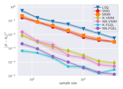
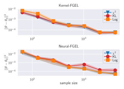
Figure 1: Estimation error over sample size for the heteroskedastic regression experiment. The left panel shows the MSE of the estimated parameters for different estimation methods. The right panels compare the performance of the kernel (K-FGEL) and neural (NN-FGEL) estimators for different divergence functions. Lines and shaded regions represent the mean and plus and minus one standard deviation of the mean over $70$ runs respectively.

4 Experiments

For all experiments we use radial basis function kernels $k_{i}(x,x^{\prime})=\exp(-\gamma\|x-x^{\prime}\|^{2})$, $i=1,\ldots,m$ and set the bandwidth parameter $\gamma$ via the common median heuristic (Schölkopf and Smola, 2002; Garreau et al., 2018). If not stated otherwise, we tune the remaining hyperparameters of all methods by evaluating the MMR objective $\ell(\theta)=1/n^{2}\sum_{i,j=1}^{n}\psi(x_{i};\theta)^{\top}K_{ij}\psi(x_{j};\theta)$ (Zhang et al., 2021) on a validation set of the same size as the training set (refer to Section A.3 of the appendix for details). We compare the performance of our kernel- and neural network-based methods with regular least-squares (LSQ), sieve minimum distance (SMD) (Ai and Chen, 2003), kernel maximum moment restrictions (MMR) (Zhang et al., 2021) and the kernel- and neural network versions of the variational method of moments (K-VMM and NN-VMM) (Bennett and Kallus, 2020b; Bennett et al., 2020) on two conditional moment restriction problems. Code for reproducing the experimental results is available at https://github.com/HeinerKremer/Functional-GEL.

4.1 Linear Regression under Heteroskedastic Noise

We define a simple data generating process for a one-dimensional estimation problem. Let $\theta=1.7\in\mathbb{R}$ and

$$y=x^{\top}\theta+\varepsilon,\ \ \ \ x\sim\operatorname{Uniform}([-1.5,1.5]),$$

where $\varepsilon$ describes heteroskedastic noise such that $\varepsilon|x\sim\mathcal{N}(0,\sigma=5x^{2})$. We can formulate the regression task as the conditional moment restriction $E[Y-X^{\top}\theta|X]=0\ P_{X}\text{-a.s.}$. As $\varepsilon$ is a mean zero random variable, here, we can use prediction mean-squared error as an unbiased validation metric to tune the hyperparameters of all methods.

Figure 1 shows the mean-squared error (MSE) of the estimated parameters using different versions of FGEL and other state-of-the-art estimators for conditional moment restrictions in dependence on the sample size. In the left figure we treat the choice of divergence as an additional hyperparameter. We observe that both our methods yield the lowest parameter MSE and even outperform the recently proposed state-of-the-art VMM estimator (Bennett and Kallus, 2020b). In the right panels we evaluate the effect of the divergence function. We observe that while the average performance is largely independent of the choice of divergence function, a comparison with the results shown in the left figure reveals that for any fixed sample the different divergences apparently yield estimators of different quality. Thus, treating the divergence as hyperparameter and choosing the estimator with the lowest validation loss, allows us to exceed the performance of the FGEL estimator with fixed divergence. As GMM-based methods implicitly build on the $\chi^{2}$-divergence, this highlights an advantage of our method which can leverage any $f$-divergences. Note that for any fixed divergence function the performance of our FGEL estimators are roughly on par with the corresponding VMM estimators.

4.2 Instrumental Variable Regression

Table 2: Prediction MSE for the instrumental variable task. Mean and standard deviation of the mean are computed over 50 random runs and multiplied by $10$ for ease of presentation.

	LSQ	SMD	MMR	K-VMM	NN-VMM	K-FGEL	NN-FGEL
abs	$3.72\pm 0.30$	$2.97\pm 0.97$	$2.78\pm 0.60$	$0.43\pm 0.15$	$0.45\pm 0.10$	$\bf{0.17\pm 0.01}$	$0.23\pm 0.06$
step	$3.03\pm 0.03$	$0.37\pm 0.04$	$0.71\pm 0.03$	$\bf{0.31\pm 0.01}$	$0.41\pm 0.01$	$0.41\pm 0.03$	$0.34\pm 0.01$
sin	$3.28\pm 0.04$	$\bf{1.01\pm 0.06}$	$3.61\pm 0.07$	$1.55\pm 0.12$	$1.72\pm 0.11$	$1.97\pm 0.16$	$1.66\pm 0.12$
linear	$2.76\pm 0.06$	$0.97\pm 0.72$	$1.98\pm 0.38$	$0.31\pm 0.06$	$0.34\pm 0.05$	$0.32\pm 0.05$	$\bf{0.20\pm 0.03}$

We adopt a slightly modified version of the IV regression experiment of Lewis and Syrgkanis (2018), which has also been used by Bennett et al. (2020) and Zhang et al. (2021). Let the data generating process be given by

$$y=f_{0}(x)+e+\delta, x=z+e+\gamma,$$

$$z\sim\operatorname{Uniform}([-3,3]),$$

$$e\sim N(0,1), \gamma,\delta\sim N(0,0.1),$$

where $f_{0}$ is picked from the following simple functions

$$\operatorname{sin:}f_{0}(x)=\sin(x), \operatorname{abs:}f_{0}(x)=|x|,$$

$$\operatorname{linear:}f_{0}(x)=x, \operatorname{step:}f_{0}(x)=I_{\{x\geq 0\}}.$$

We approximate $f_{0}$ by a shallow neural network $f_{\theta}(x)$ with 2 layers of $[20,3]$ units and leaky ReLU activation functions and base the estimation on the conditional moment restrictions $E[Y-f_{\theta}(X)|Z]=0\ \ P_{Z}\text{-a.s.}$. As generally the true model is not contained in this model class, this provides a typical case of model mis-specification and theoretical properties of the our method (and equally all baseline methods) for this setting have yet to be developed (see Dikkala et al. (2020) for recent progress in this direction). We use training and validation sets of size $n=2000$ and evaluate the prediction error on a test set of $20000$ samples. The results are visualized in Table 2. We observe that with the exception of one task the FGEL and VMM estimators outperform all other baselines. Compared to each other NN-FGEL seems to be preferable over NN-VMM but the kernel versions of both methods exhibit similar performance without showing a clear advantage of one over the other for this task.

Our experiments show that the FGEL estimator is a viable alternative to previously proposed continuum method of moments estimators for conditional moment restrictions and can surpass the previous state-of-the-art on some tasks. However, further empirical evidence needs to be collected to verify its predicted superior finite sample properties for infinitely many moment restrictions. We leave a comprehensive experimental evaluation to future work.

5 Related Work

Learning with conditional or infinite dimensional moment restrictions respectively has been an active field of research in econometrics and more recently in machine learning. In the former context, seminal work on extending the generalized method of moments to continua of moment restrictions has been carried out by Carrasco and Florens (2000); Carrasco et al. (2007) by placing the constraints in an RKHS. In the machine learning community, GMM-related estimators have been developed by casting the infinite dimensional moment restriction problem as a minimax game and representing the adversarial player by an RKHS function (Zhang et al., 2021; Bennett and Kallus, 2020b) or a flexible neural network (Hartford et al., 2017; Lewis and Syrgkanis, 2018; Dikkala et al., 2020; Bennett et al., 2020). While the neural network-based methods often achieve good performance in practice, they generally are computationally more expensive and lack the theoretical properties of traditional GMM estimators. In contrast, Bennett and Kallus (2020b)’s kernel-VMM estimator comes with strong theoretical guarantees but results from a 2-step procedure and thus depends on an initial parameter estimate. As discussed in Section 3.6, our framework contains a continuous updating version of VMM as a special case but allows for using alternative $f$-divergence functions.

As an alternative to GMM estimation, sieve-based methods (Newey and Powell, 2003; Donald et al., 2003; Ai and Chen, 2003; Chen and Pouzo, 2012) address conditional moment restrictions by growing the number of unconditional restrictions with the sample size by manually selecting an increasing number of basis functions. While these often come with desirable efficiency results, in practice they can be hard to tune and computationally demanding (Bennett and Kallus, 2020b). Another line of work implicitly estimates optimal instrument functions via a kernel-smoothed localized empirical likelihood function (Tripathi and Kitamura, 2003; Kitamura et al., 2004). Their use of kernels is very different from our approach as we do not smooth the profile divergence but use RKHS functions as instrument functions.

Several works extended the generalized empirical likelihood framework to handle infinite dimensional moment restrictions and thus conditional moment restrictions (Donald et al., 2003; Chaussé, 2012; Carrasco and Kotchoni, 2017). The GEL estimator of Chaussé (2012) is based on approximately imposing a continuum of moment restrictions using a parameterized basis of functions and solving a regularized version of the GEL first order conditions. While it is theoretically closely related to our method, the regularization scheme and computational approach differs from ours. Similarly, closely related to our method is the regularized GEL estimator of Carrasco and Kotchoni (2017), which is defined via a set of optimality conditions and solved using a procedure motivated by the Three-Steps Euclidean Likelihood procedure of Antoine et al. (2007). In contrast to these methods, our estimator is defined as a saddle point of an objective function and thus benefits from recent advances in mini-max optimization (Daskalakis et al., 2018; Lin et al., 2020). To the best of our knowledge, our work is the first to combine GEL estimation with modern machine learning and in particular kernel methods and neural networks.

6 Conclusion

Several long-established problems in machine learning can naturally be expressed as a risk minimization problem. On the other hand, emerging areas such as causal inference, algorithmic decision making, and robust learning often involve problems that are formulated as (potentially infinite) moment restrictions and require different algorithmic frameworks for estimation and inference. Recent works have advanced this development by combining classical techniques from econometrics such as generalized method of moments (GMM) with modern machine learning models such as deep neural networks and kernel machines. Likewise, our work contributes to this endeavour by equipping the more general generalized empirical likelihood (GEL) framework with such powerful models. While the econometrics community enjoys the new class of algorithms, we believe the machine learning community will likewise benefit from new perspectives on causal inference and robust learning which will be explored in future works.

This paper laid the theoretical foundation of the functional GEL framework, but there remain open questions that impede real-world applications. Firstly, more efficient optimization procedures need to be developed that allow for large scale applications. Secondly, theoretical properties of the framework with specific function classes need to be explored. Lastly, the framework needs to be tested for the training of more complex models for real-world applications (e.g. robust learning). Our goal is to address some of these problems in future work.

Appendix A Additional Information

A.1 Distributional Robustness of FGEL

It is well-known that the profile divergence is a dual formulation to the distributionally robust optimization (DRO) formulation Lam [2019], Duchi et al. [2018]. In the context of this paper, one can show that $R_{\lambda_{n}}(\theta)\leq\rho$ if and only if

$$\lambda_{n}\geq\inf_{P\in\mathcal{P}}\|E_{P}[H(X,Z;\theta)]\|_{\mathcal{H}^{\ast}}\;\ \mathrm{s.t.}\,D_{f}(P||\hat{P}_{n})\leq\rho.$$

However, we do not simply rely on the divergence-ball centered at the empirical data distribution $\{P|\ D_{f}(P||\hat{P}_{n})\leq\rho\}$ (referred to as an ambiguity set in the DRO literature) for robustness. Since that robustness is often used to account for the statistical error due to finite samples. Instead, we are concerned with a second and stronger layer of robustness.

First, note that the quantity $E_{P}[H(X,Z;\theta)]$ is used to approximate the conditional moment constraint in our original formulation (8). Since the goal of FGEL is to satisfy the the conditional moment restrictions $E_{P}[\psi(X;\theta)\,|\,Z]=0$ almost everywhere in the domain, in robust optimization terms, we are robustifying against the instrument $Z$. The instrument $Z$ can create much stronger distribution shifts in the data-generating process than the mere statistical fluctuation described by divergence-ball-based DRO works following Ben-Tal et al. [2013] and Duchi et al. [2018]. We leave an alternative DRO algorithm against such strong distribution shifts for future work.

From another perspective, our method can also be seen as enforcing independence between $Z$ and the moment restriction, e.g., for IV regression the residual $\psi(X;\theta)=Y-f_{\theta}(X)$. Intuitively, we want the residual $Y-f_{\theta}(X)$ to be small and invariant to transformations of the $Z$ variable (marginal shift). This kind of robust learning strategy has also been studied in works such as Greenfeld and Shalit [2020], Rothenhäusler et al. [2020], Heinze-Deml and Meinshausen [2019].

A.2 Computing the FGEL Estimator

Problem (13) is generally a non-convex-convex min-max problem in the parameter $\theta$ and function $h$. Let $h=h_{\alpha}$ be described by a finite dimensional set of parameters $\alpha\in A$, which is the case, e.g., for neural network function classes or RKHS after using a representer theorem. Furthermore let the set of parameters $A$ be compact. If additionally the parameterization leaves the convexity of the inner problem intact (e.g., in the case of kernel-FGEL) we can use a simplified version of Danskin’s theorem [Danskin, 1966] to compute gradients of $R_{\lambda_{n}}(\theta):=\sup_{h\in\widehat{\mathcal{H}}_{\theta}}G_{\lambda_{n}}(\theta,h)$ in a principled way.

Lemma A.1 (Danskin).

Let $\hat{h}(\theta)$ denote the solution of the inner convex optimization over $h\in\mathcal{H}_{\theta}$ such that $\hat{h}(\theta)=\operatorname*{arg\,max}_{h\in\widehat{\mathcal{H}}_{\theta}}G_{\lambda_{n}}(\theta,h)$. Then the gradient of the profile divergence $R_{\lambda_{n}}(\theta)$ with respect to the parameters $\theta\in\Theta$ is given by

$$\nabla R_{\lambda_{n}}(\theta)=\nabla G_{\lambda_{n}}(\theta,\hat{h}(\theta)).$$

Therefore, we can adopt a gradient-based strategy for the outer optimization problem over $\theta$ using in each step the gradient estimate obtained from the solution of the inner maximization over $h$. Depending on the GEL function $\phi$ the optimization of both, the outer and inner problem can then be solved efficiently with an off-the-shelf solver e.g. using LBFGS (cf. Algorithm 1).

Algorithm 1 Kernel-FGEL

  Input: data $(x_{i},y_{i},z_{i})$, hyperparameter $\lambda$

  while not converged do

     while not converged do

        $\alpha\leftarrow\operatorname{LBFGS}(G_{\lambda}(\theta,h_{\alpha}))$

     end while

     $\theta\leftarrow\operatorname{LBFGS}(G_{\lambda}(\theta,h_{\alpha}))$

  end while

  Output: Parameter estimate $\theta$

For the case of a neural network instrument function classes, we build on the recent progress in mini-max optimization and employ the optimistic Adam optimizer [Daskalakis et al., 2018] which has been developed to solve similar saddle point problems for training generative adversarial networks [Goodfellow et al., 2014] (cf. Algorithm 2). Implementations of both approaches are available under https://github.com/HeinerKremer/Functional-GEL.

Algorithm 2 Neural-FGEL

  Input: data $(x_{i},y_{i},z_{i})$, hyperparameter $\lambda$

  while not converged do

     $\alpha\leftarrow\operatorname{OAdam}(G_{\lambda}(\theta,h_{\alpha}))$

     $\theta\leftarrow\operatorname{OAdam}(G_{\lambda}(\theta,h_{\alpha}))$

  end while

  Output: Parameter estimate $\theta$

A.3 Hyperparameter selection

Tuning the hyperparameter of our method, i.e., the regularization parameter $\lambda_{n}$ (and, e.g., learning rates) requires a data-driven performance measure of the obtained model parameters. We know that for the true distribution $P_{0}$ and true parameter $\theta_{0}$ we obtain $\|E_{P_{0}}[H(X,Z;\theta_{0})]\|_{\mathcal{H}^{\ast}}^{2}=0$. Let $\beta$ denote the set of hyperparameters and $\hat{\theta}(\beta)$ the corresponding solution to (13). Then we can define a performance measure of the solution candidate $\hat{\theta}(\beta)$ as $\ell(\beta)=\|E_{P_{0}}[H(X,Z;\hat{\theta}(\beta))]\|_{\mathcal{H}^{\ast}}^{2}$. As we do not have access to the true distribution $P_{0}$ we can define a natural surrogate loss $\hat{\ell}$ using a validation set with empirical distribution $\hat{P}_{\text{val}}$ as

$$\hat{\ell}(\beta)=\|E_{\hat{P}_{\text{val}}}H(X,Z;\hat{\theta}(\beta))\|_{\mathcal{H}^{\ast}}^{2}$$ (16)

Choosing $\mathcal{H}$ as an RKHS, this can be expressed as the kernel maximum of moment restriction objective of Muandet et al. [2020] and Zhang et al. [2021] evaluated on the validation data as shown by the following lemma.

Lemma A.2.

Let $\{x_{i},z_{i}\}_{i=1}^{n}$ denote the validation data and define $\boldsymbol{\psi}_{j}(\boldsymbol{x};\theta)=\operatorname{vec}(\{\psi_{j}(x_{i};\theta)\}_{i=1}^{n})$. Let $K_{j}$ denote the kernel Gram matrix with entries $\left(K_{j}\right)_{pq}=k_{j}(z_{p},z_{q})$, $p,q=1,\ldots,n$, $j=1,\ldots,m$. Then we can express (16) as

$$\hat{\ell}(\beta)=\frac{1}{n^{2}}\sum_{j=1}^{m}\boldsymbol{\psi}_{j}(\boldsymbol{x};\theta)^{T}K_{j}\boldsymbol{\psi}_{j}(\boldsymbol{x};\theta).$$ (17)

Here we assume that possible hyperparameters of the kernel are already set via commonly employed heuristics like the median heuristic [Schölkopf and Smola, 2002, Garreau et al., 2018] for the kernel bandwidth and only tune the remaining parameters of our method.

Appendix B Proofs

B.1 Preliminaries

For ease of notation we define some expressions first. Define $H_{i}(\theta):=H(x_{i},z_{i};\theta)$ and denote $\phi_{i}(v)=\frac{d^{i}}{(dv)^{i}}\phi(v)$ and $\phi_{i}=\phi_{i}(0)$. Without loss of generality we assume that $\phi_{1}(0)=\phi_{2}(0)=-1$, as any $\phi$ with $\phi_{1}\neq 0$ and $\phi_{2}<0$ can be rescaled to achieve this (see Newey and Smith [2004]). Define the empirical objective as $\widehat{G}_{\lambda_{n}}(\theta,h)=\sum_{i=1}^{n}\phi(H(x_{i},z_{i};\theta)(h))-\lambda\|h\|_{\mathcal{H}}^{2}$ and the empirical constraint set as $\widehat{\mathcal{H}}_{n}(\theta)=\{h\in\mathcal{H}:H(x_{i},z_{i};\theta)(h)\in\operatorname{dom}(\phi)\ \ \forall(x_{i},z_{i}),\ i=1,\ldots,n\}$. Throughout the proofs we will make use of functional derivatives and a functional version of Taylor’s theorem with Lagrange remainder, which we define and state next, respectively.

Definition B.1 (Functional Derivative).

Let $\mathcal{H}$ be a vector space of functions. For a functional $G:\mathcal{H}\rightarrow\mathbb{R}$ and a pair of functions $h,\tilde{h}\in\mathcal{H}$, we define the derivative operator $D_{h}G(h)[\tilde{h}]=\left.\frac{d}{dt}G(h+t\tilde{h})\right|_{t=0}$. Likewise, we define

$$D_{h}^{k}G(h)\left[h_{1},\ldots,h_{k}\right]=\left.\frac{\partial^{k}}{\partial t_{1}\ldots\partial t_{k}}G\left(h+t_{1}h_{1}+\ldots+t_{k}h_{k}\right)\right|_{t_{1}=\cdots=t_{k}=0}.$$

Similarly, when considering a function of a vector-valued parameter, $G:\Theta\subseteq\mathbb{R}^{p}\rightarrow\mathbb{R}$, we denote the $k$-th standard directional derivative at $\theta\in\Theta$ as $D^{k}_{\theta}G(\theta)(\theta_{1},\ldots,\theta_{k})$.

Proposition B.2 (Taylor’s theorem).

Let $G:\mathcal{H}\rightarrow\mathbb{R}$, where $\mathcal{H}$ is a vector space of functions. For any $h,h^{\prime}\in\mathcal{H}$, if $t\mapsto G\left(th+(1-t)h^{\prime}\right)$ is $(k+1)$-times differentiable over an open interval containing $[0,1]$, then there exists $\bar{h}\in\operatorname{conv}\left(\left\{h,h^{\prime}\right\}\right)$ such that

$$G\left(h^{\prime}\right)= \ G(h)+\sum_{i=1}^{k}\frac{1}{i!}D_{h}^{i}G(h)[\underbrace{h^{\prime}-h,\ldots,h^{\prime}-h}_{i\text{ times }}]$$

$$+\frac{1}{(k+1)!}D_{h}^{k+1}G(\bar{h})[\underbrace{h^{\prime}-h,\ldots,h^{\prime}-h}_{k+1\text{ times }}].$$

Equally, using the notation of Definition B.1 the same result holds for functions of vector-valued parameters $G:\Theta\subseteq\mathbb{R}^{p}\rightarrow\mathbb{R}$.

Our duality result builds on Theorem 3.1 of Borwein [1993]. For completeness, we will state it here adapted to our notation. Note that while the theorem is already closely related to our result, a direct application of the theorem to our case is impeded as we additionally need to take into account the normalization constraint for $p$, i.e., $\sum_{i=1}^{n}p_{i}=1$.

Proposition B.3 (Borwein’s theorem).

Consider the problem ((10) without the normalization of $p$)

$$P=\inf_{p\in\mathbb{R}^{n}}\sum_{i=1}^{n}\frac{1}{n}f(np_{i})\quad\mathrm{s.t.}\ \ \|\frac{1}{n}\sum_{i=1}^{n}p_{i}H(x_{i},z_{i};\theta)\|_{\mathcal{H}^{\ast}}=0$$ (18)

and assume the infimum is attained (when finite). Consider for $\lambda>0$ the relaxed problem

$$P_{\lambda}=\min_{p\in\mathbb{R}^{n}}\sum_{i=1}^{n}\frac{1}{n}f(np_{i})\quad\mathrm{s.t.}\ \ \|\frac{1}{n}\sum_{i=1}^{n}p_{i}H(x_{i},z_{i};\theta)\|_{\mathcal{H}^{\ast}}\leq\lambda.$$ (19)

Then the value $P_{\lambda}$ equals the value of the dual program

$$D_{\lambda}=\max_{h\in\mathcal{H}}-\frac{1}{n}\sum_{i=1}^{n}f^{\ast}(H(x_{i},z_{i};\theta)(h))-\lambda\|h\|_{\mathcal{H}},$$ (20)

and the unique optimal solution of (19) is given by

$$(p_{\lambda})_{i}=\left(\frac{d}{dv}f^{\ast}\right)\left(H(x_{i},z_{i};\theta)(\hat{h})\right),\quad i=1,\ldots,n,$$

where $\hat{h}$ is any solution of (20). Moreover, as $\lambda\rightarrow 0$, $p_{\lambda}$ converges in mean to unique solution of (18) and $P_{\lambda}\rightarrow P$.

Proof of Theorem 3.1

Proof.

The proof follows almost directly from application of Proposition B.3 by taking into account the additional constraint $\sum_{i=1}^{n}p_{i}=1$.

The dual problem can be derived by introducing Lagrange parameters $\nu>0$ and $\mu\in\mathbb{R}$ and defining the Lagrangian

$$L(\theta,p,\mu,\nu)=\sum_{i=1}^{n}\frac{1}{n}f(np_{i})-\mu\left(\sum_{i=1}^{n}p_{i}-1\right)+\nu\left(\|\sum_{i=1}^{n}p_{i}H(x_{i},z_{i};\theta)\|_{\mathcal{H}^{\ast}}-\lambda\right).$$

Using the definition of the dual norm and the fact that trivially $\lambda=\max_{\|h\|=1}\|h\|\lambda=\min_{\|h\|=1}\|h\|\lambda$, we have

$$L=\sum_{i=1}^{n}\frac{1}{n}f(np_{i})-\mu\left(\sum_{i=1}^{n}p_{i}-1\right)+\sup_{\|\tilde{h}\|_{\mathcal{H}}=1}\left(\sum_{i=1}^{n}\langle\nu\tilde{h},p_{i}H(x_{i},z_{i};\theta)\rangle-\|\nu\tilde{h}\|_{\mathcal{H}}\lambda\right).$$

By defining new dual Lagrange parameters $h=\nu\tilde{h}\in\mathcal{H}$, we thus obtain

$$L(\theta,p,\mu,h)=\sum_{i=1}^{n}\frac{1}{n}f(np_{i})-\mu\left(\sum_{i=1}^{n}p_{i}-1\right)+\sum_{i=1}^{n}\langle h,p_{i}H(x_{i},z_{i};\theta)\rangle-\|h\|_{\mathcal{H}}\lambda.$$

Now, redefining $p_{i}\rightarrow np_{i}$ and optimizing the Lagrangian with respect to p we get

$$\min_{p}\Big{\{}\mu-\frac{1}{n}\sum_{i=1}^{n}\Big{[}(\mu-H(x_{i},z_{i};\theta)(h))p_{i}-f(p_{i})\Big{]}-\lambda\|h\|_{\mathcal{H}}\Big{\}}$$

$$= \ \mu-\frac{1}{n}\sum_{i=1}^{n}\max_{p_{i}}\Big{\{}(\mu-H(x_{i},z_{i};\theta)(h))p_{i}-f(p_{i})\Big{\}}-\lambda\|h\|_{\mathcal{H}}$$

$$= \ \mu-\frac{1}{n}\sum_{i=1}^{n}f^{\ast}(\mu-H(x_{i},z_{i};\theta)(h))-\lambda\|h\|_{\mathcal{H}},$$

where we used the definition of the Legrendre-Fenchel (convex) conjugate function $f^{\ast}(v)=\sup_{x}\langle v,x\rangle-f(x)$. As for any $h\in\mathcal{H}$, $-h\in\mathcal{H}$, we can redefine $h\rightarrow-h$ and finally obtain the result. Finally from Proposition B.3 it follows that strong duality holds and the unique minimizer of the primal problem is given by

$$p_{i}=\left(\frac{d}{dv}f^{\ast}\right)\left(H(x_{i},z_{i};\theta)(\hat{h})+\hat{\mu}\right),\quad i=1,\ldots,n,$$

where $\hat{h}$, $\hat{\mu}$ are any solutions of the dual problem. ∎

B.2 Proof of Theorem 3.6

For the proof of Lemma B.5 we will need the following result whose proof closely follows a similar result for vector-valued moment restrictions of Owen [1990] and Kitamura et al. [2004] (Lemma D.2):

Lemma B.4.

Let X be a RV taking values in $\mathcal{X}$, for a bounded functional $H:\mathcal{X}\times\Theta\times\mathcal{H}\rightarrow\mathbb{R}$ with $E\left[\left(\sup_{\theta\in\Theta}\|H(X;\theta)\|_{\mathcal{H}^{\ast}}\right)^{m}\right]<\infty$, it follows that $\max_{1\leq j\leq n}\sup_{\theta\in\Theta}\left\|H\left(x_{j};\theta\right)\right\|_{\mathcal{H}^{\ast}}=o\left(n^{1/m}\right)$ with probability 1.

Proof.

For ease of notation define the random variable $Y:=\sup_{\theta\in\Theta}\left\|H\left(X;\theta\right)\right\|$ and let for $i\in\mathbb{N}$, $Y_{i}$ denote independent copies of $Y$. Then as $E[Y^{m}]\leq\infty$, we must have that $\sum_{i=1}^{\infty}P(Y_{i}^{m}>n)<\infty$ or equivalently $\sum_{i=1}^{\infty}P(Y_{i}>n^{1/m})<\infty$. Hence by the Borel-Cantelli Lemma the event $Y_{i}>n^{1/m}$ happens only finitely often with probability $1$ which likewise implies $Z_{n}:=\max_{1\leq i\leq n}Y_{i}>n^{1/m}$ happens only finitely often with probability $1$. By the same argument the event $Z_{n}=\epsilon n^{1/m}$ happens only finitely often for any $\epsilon>0$ and thus

$$\limsup Z_{n}/n^{1/m}\leq\epsilon$$

with probability $1$ and thus $Z_{n}=o(n^{1/m})$ with probability $1$. ∎

The following Lemma shows that if we constrain the space of the dual parameter to a ball of radius $\zeta$ with $1/\nu<\zeta<1/2-\xi$, the largest value the empirical moment functional evaluated on the dual parameter can take converges to zero in probability. Furthermore any such ball is contained in the empirical constraint set $\widehat{\mathcal{H}}_{n}(\theta)$.

Lemma B.5.

Let the assumptions of Theorem 3.6 be satisfied, then for any $\zeta$ with $1/\nu<\zeta<1/2-\xi$ define $\mathcal{H}_{n}=\{h:\|h\|_{\mathcal{H}}\leq n^{-\zeta}\}$. Then $\sup_{\theta\in\Theta,h\in\mathcal{H}_{n},1\leq i\leq n}|H(x_{i},z_{i};\theta)(h)|\overset{p}{\rightarrow}0$ and w.p.a.1, $\mathcal{H}_{n}\subseteq\widehat{\mathcal{H}}_{n}(\theta)$ for all $\theta\in\Theta$.

Proof.

Using the Cauchy-Schwarz inequality together with Lemma B.4 we have

$$\sup_{\theta\in\Theta,h\in\mathcal{H}_{n},1\leq i\leq n}|H(x_{i},z_{i};\theta)(h)|$$

$$\leq\sup_{\theta\in\Theta,h\in\mathcal{H}_{n},1\leq i\leq n}\left(\|h\|_{\mathcal{H}}\cdot\|H(x_{i},z_{i};\theta)\|_{\mathcal{H}^{\ast}}\right)$$

$$\leq n^{-\zeta}\sup_{\theta\in\Theta,1\leq i\leq n}\|H(x_{i},z_{i};\theta)\|_{\mathcal{H}^{\ast}}$$

$$=O_{p}(n^{-\zeta+1/\nu})\overset{p}{\rightarrow}0.$$

As $V=\operatorname{dom}(\phi)$ is an open interval containing zero it follows that $H(x_{i},z_{i};\theta))(h)\in\operatorname{dom}(\phi)$ w.p.a.1 for all $\theta\in\Theta$ and $h\in\mathcal{H}_{n}$. ∎

Next we assume we have an estimator $\bar{\theta}$ that converges to the solution $\theta_{0}$ in probability and for which the empirical moment functional converges to 0 in the dual norm. We show that then the inner maximization of the regularized empirical objective $\widehat{G}_{\lambda_{n}}(\theta,h)$ (with the empirical constraint set $\widehat{\mathcal{H}}_{n}(\theta)$) over the dual function $h$ has a solution w.p.a.1 which converges to 0 in the function space norm. Likewise the unregularized empirical objective evaluated at this solution converges to $\phi(0)$. The proof generalizes Lemma A2 of Newey and Smith [2004] to our regularized continuum formulation. It is different from a similar proof in Chaussé [2012] (Lemma 2), as our regularization procedure differs from theirs.

Lemma B.6.

Let the assumptions of Theorem 3.6 be satisfied. Additionally let $\bar{\theta}\in\Theta$, $\bar{\theta}\overset{p}{\rightarrow}\theta_{0}$, and $\|E_{\hat{P}_{n}}[H(X,Z;\bar{\theta})]\|_{\mathcal{H}^{\ast}}=O_{p}\left(n^{-1/2}\right)$, further let $\lambda_{n}=O_{p}(n^{-\xi})$ where $0<\xi<1/2-1/\nu$. Then $\bar{h}=$ $\operatorname*{arg\,max}_{h\in\widehat{\mathcal{H}}_{n}(\bar{\theta})}\widehat{G}_{\lambda_{n}}(\bar{\theta},h)$ exists w.p.a.1, $\|\bar{h}\|_{\mathcal{H}}=O_{p}\left(n^{-1/2+\xi}\right)$, and $\widehat{G}_{\lambda_{n}}(\bar{\theta},\bar{h})\leq\phi(0)+O_{p}\left(n^{-1+2\xi}\right)$.

Proof.

Let $\bar{H}_{i}:=H_{i}(\bar{\theta})$ and $\bar{H}=\frac{1}{n}\sum_{i=1}^{n}\bar{H}_{i}$. Let $\widehat{\Omega}(\theta)=\frac{1}{n}\sum_{i=1}^{n}H(x_{i},z_{i};\theta)\otimes H(x_{i},z_{i};\theta)$ denote the empirical covariance operator evaluated at $\theta$. By Lemma B.5 and twice continuous differentiability of $\phi(v)$ in a neighborhood of zero, $\widehat{G}_{\lambda_{n}}(\bar{\theta},h)$ is twice continuously differentiable on $\mathcal{H}_{n}$ w.p.a.1., with $\mathcal{H}_{n}=\{h:\|h\|_{\mathcal{H}}\leq n^{-\zeta}\}$ as in Lemma B.5. Then $\tilde{h}=\operatorname*{arg\,max}_{h\in\mathcal{H}_{n}}\widehat{G}_{\lambda_{n}}(\bar{\theta},h)$ exists w.p.a.1. Using Taylor’s theorem (Proposition B.2) we can expand the regularized GEL objective about $h=0$ and obtain

$$\phi_{0} =\widehat{G}_{\lambda_{n}}(\bar{\theta},0)$$

$$\leq\widehat{G}_{\lambda_{n}}(\bar{\theta},\tilde{h})$$

$$=\phi_{0}-\bar{H}(\tilde{h})$$

$$+\frac{1}{2}\left[\frac{1}{n}\sum_{i=1}^{n}\phi_{2}(\bar{H}_{i}(\dot{h}))(\bar{H}_{i}\otimes\bar{H}_{i})-\lambda_{n}I\otimes I\right](\tilde{h},\tilde{h})$$

for some $\dot{h}$ on the line between $0$ and $\tilde{h}$. With Lemma B.5 and $\phi_{2}(0)=-1$ we have that $\max_{1\leq i\leq n}\phi_{2}(\bar{H}_{i}(\dot{h}))<-1/2$ w.p.a.1. Using this and subtracting $\phi_{0}$ on both sides yields

$$0\leq-\bar{H}(\tilde{h})-\frac{1}{4}(\widehat{\Omega}(\bar{\theta})+2\lambda_{n}I\otimes I)(\tilde{h},\tilde{h})$$

By the uniform weak law of large numbers we have $\widehat{\Omega}(\bar{\theta})\overset{p}{\rightarrow}\Omega(\bar{\theta})$. As $\Omega(\theta)$ is a positive semi-definite compact operator for all $\theta$, its smallest eigenvalue is not bounded away from zero. However, with $\lambda_{n}>0$ the smallest eigenvalue $C_{\lambda_{n}}$ of $\widehat{\Omega}(\bar{\theta})+2\lambda_{n}I\otimes I$ is bounded away from zero, i.e., $C_{\lambda_{n}}>0$ w.p.a.1, and $O_{p}(\lambda_{n})$. Inserted in above inequality we get

$$0 \leq-\bar{H}(\tilde{h})-\frac{1}{4}(\widehat{\Omega}(\bar{\theta})+2\lambda_{n}I\otimes I)(\tilde{h},\tilde{h})$$

$$\leq\|\bar{H}\|_{\mathcal{H}^{\ast}}\|\tilde{h}\|_{\mathcal{H}}-C_{\lambda_{n}}\|\tilde{h}\|_{\mathcal{H}}^{2},$$

where in the second line we used the Cauchy-Schwarz inequality for the first term. This means we have $C\|\tilde{h}\|_{\mathcal{H}}\leq\|\bar{H}\|_{\mathcal{H}^{\ast}}$ w.p.a.1. As by assumption $\|\bar{H}\|=O_{p}(n^{-1/2})$ it follows that $\|\tilde{h}\|=O_{p}(\lambda_{n}^{-1}n^{-1/2})=O_{p}(n^{-\zeta})$, with $\zeta=1/2-\xi$. Now, as $0<\xi<1/2-1/\nu$, we have $1/\nu<\zeta<1/2$ and and therefore $\tilde{h}\in\operatorname{int}(\mathcal{H}_{n})$ w.p.a.1. Moreover, as $\tilde{h}$ is a maximizer contained in the interior of the domain $\mathcal{H}_{n}$, it must correspond to a stationary point of $\widehat{G}_{\lambda_{n}}$, i.e., $\partial\widehat{G}_{\lambda_{n}}(\bar{\theta},\tilde{h})/\partial h=0$. However, from Lemma B.5 it follows that w.p.a.1 $\tilde{h}\in\widehat{\mathcal{H}}_{n}(\bar{\theta})$ and as $\widehat{G}_{\lambda_{n}}(\bar{\theta},h)$ is concave and $\widehat{\mathcal{H}}_{n}(\bar{\theta})$ is convex we must have $\widehat{G}_{\lambda_{n}}(\bar{\theta},\tilde{h})=\sup_{h\in\widehat{\mathcal{H}}_{n}(\bar{\theta})}\widehat{G}_{\lambda_{n}}(\bar{\theta},h)$, which directly implies $\bar{h}=\tilde{h}$ and proves the first conclusion. The second conclusion follows directly as $\bar{h}\in\operatorname{int}(\mathcal{H}_{n})$ and thus $\bar{h}=O_{p}(n^{-\zeta})$. Finally as $\|\bar{H}\|_{\mathcal{H}^{\ast}}=O_{p}(n^{-1/2})$ by assumption, we have $\widehat{G}_{\lambda_{n}}(\bar{\theta},\bar{h})\leq\phi_{0}+\|\bar{H}\|_{\mathcal{H}^{\ast}}\|\bar{h}\|_{\mathcal{H}}-C\|\bar{h}\|_{\mathcal{H}}^{2}=\phi_{0}+O_{p}\left(n^{-1+2\xi}\right)$, which completes the proof. ∎

The following lemma which builds on Lemma B.5 and B.6 shows that the empirical moment functional $\frac{1}{n}\sum_{i=1}^{n}H_{i}(\hat{\theta})$ evaluated at the FGEL estimator $\hat{\theta}$ converges to zero in the dual norm. The proof is almost identical to the one provided by Newey and Smith [2004] (Lemma A3) but takes into account the regularized rates. Note that Chaussé [2012] provides a slightly different and shortened version of this proof.

Lemma B.7.

Let the assumptions of Theorem 3.6 be satisfied and denote $\hat{\theta}$ the corresponding FGEL estimator $\hat{\theta}=\operatorname*{arg\,min}_{\theta\in\Theta}\sup_{h\in\widehat{\mathcal{H}}_{n}(\bar{\theta})}\widehat{G}_{\lambda_{n}}({\theta},h)$. Then $\|E_{\hat{P}_{n}}[H(X,Z;\hat{\theta})]\|_{\mathcal{H}^{\ast}}=O_{p}\left(n^{-1/2+\xi}\right)$.

Proof.

Similarly as is in the proof of Lemma B.6, define $\hat{H}_{i}:=H_{i}(\hat{\theta})$ and $\hat{H}=\frac{1}{n}\sum_{i=1}^{n}\hat{H}_{i}$. Let $\mu(\hat{H})$ be the Riesz representer of $\hat{H}\in\mathcal{H}^{\ast}$ in $\mathcal{H}$. Further, let $\zeta$ be defined as in Lemma B.5 and consider $\tilde{h}=-n^{-\zeta}\mu(\hat{H})/\|\mu(\hat{H})\|_{\mathcal{H}}$, which implies $\tilde{h}\in\mathcal{H}_{n}$ and therefore by Lemma B.5 $\max_{1\leq i\leq n}\|\hat{H}(\tilde{h})\|\overset{p}{\rightarrow}0$ and $\tilde{h}\in\widehat{\mathcal{H}}_{n}$ w.p.a.1. Using the same steps as in the proof of Lemma B.6 we can Taylor expand the empirical FGEL objective about $h=0$,

$$\widehat{G}_{\lambda_{n}}(\hat{\theta},\tilde{h})=\phi(0)-\hat{H}(\tilde{h})$$

$$+\frac{1}{2}\left[\frac{1}{n}\sum_{i=1}^{n}\phi_{2}(\hat{H}_{i}(\dot{h}))(\hat{H}_{i}\otimes\hat{H}_{i})-\lambda_{n}I\otimes I\right](\tilde{h},\tilde{h}),$$

for some $\dot{h}$ on the line between 0 and $\tilde{h}$. Note that for any $\dot{h}$ on the line between $0$ and $\tilde{h}$ we have $\phi_{2}(\hat{H}_{i}(\dot{h}))\geq-C_{1}$, $i=1,\ldots,n$, for some constant $C_{1}>0$. Further, as the covariance operator is a compact operator, its largest eigenvalue can be bounded by a constant $C_{2}>0$. Putting this together, the third term above can be bounded by $-C\|\tilde{h}\|^{2}_{\mathcal{H}}$, where $C>0$ is another constant. Therefore, we have w.p.a.1,

$$\widehat{G}_{\lambda_{n}}(\hat{\theta},\tilde{h})\geq\phi(0)+n^{-\zeta}\|\hat{H}\|_{\mathcal{H}^{\ast}}-Cn^{-2\zeta},$$

where for the second term we have used the definition of $\tilde{h}$. Consider $\bar{\theta}=\theta_{0}$ in Lemma B.6, for which the requirements are fulfilled as with $\|E[H(X,Z;{\theta_{0}})]\|_{\mathcal{H}^{\ast}}=0$, by the central limit theorem we have that $\|E_{\hat{P}_{n}}[H(X,Z;{\theta_{0}})]\|_{\mathcal{H}^{\ast}}=O_{p}\left(n^{-1/2}\right)$. Moreover, being the solution to the mini-max problem, $(\hat{\theta},\hat{h})$ correspond to a saddle point of the empirical FGEL objective $\widehat{G}_{\lambda_{n}}$. Using this and Lemma B.6 we have

$$\phi(0)+n^{-\zeta}\|\hat{H}\|_{\mathcal{H}^{\ast}}-Cn^{-2\zeta}\leq\widehat{G}_{\lambda_{n}}(\hat{\theta},\tilde{h})$$

$$\leq \ \widehat{G}_{\lambda_{n}}(\hat{\theta},\hat{h})$$

$$\leq \sup_{h\in\widehat{\mathcal{H}}_{n}}\widehat{G}_{\lambda_{n}}(\theta_{0},h)\leq\phi(0)+O_{p}(n^{-1+2\xi}).$$

Now, subtracting $\phi(0)$ on both sides and solving for $\|\hat{H}\|_{\mathcal{H}^{\ast}}$, we obtain

$$\|\hat{H}\|_{\mathcal{H}^{\ast}}\leq O_{p}(n^{\zeta-1+2\xi})+Cn^{-\zeta}=O_{p}(n^{-\zeta}),$$ (21)

which follows as $\zeta<1/2-\xi$ and therefore $\zeta-1+2\xi<\xi-1/2\leq-\zeta$. Consider any $\epsilon_{n}\rightarrow 0$ and let $\tilde{h}=-\epsilon_{n}\mu(\hat{H})$. Then by (21), $\tilde{h}=o_{p}(n^{-\zeta})$ and therefore $\tilde{h}\in\mathcal{H}_{n}$ w.p.a.1. Then as previously we have

$$\phi(0)-\hat{H}(\tilde{h})-C\|h\|_{\mathcal{H}}^{2}$$

$$= \ \phi(0)+\epsilon_{n}\|\hat{H}\|_{\mathcal{H}^{\ast}}^{2}-C\epsilon_{n}^{2}\|\hat{H}\|_{\mathcal{H}^{\ast}}^{2}$$

$$\leq \ \phi(0)+O_{p}(n^{-1+2\xi}).$$

As $1-\epsilon_{n}C$ is bounded away from zero, for all $n$ large enough, we have $\epsilon_{n}\|\hat{H}\|_{\mathcal{H}^{\ast}}^{2}=O_{p}(n^{-1+2\xi})$. As this holds for all $\epsilon_{n}\rightarrow 0$, it follows that $\|\hat{H}\|_{\mathcal{H}^{\ast}}=O_{p}(n^{-1/2+\xi})$. ∎

Proof of Theorem 3.6

Proof.

Define $\hat{H}_{i}=H(x_{i},z_{i};\hat{\theta})$ and $\hat{H}=\frac{1}{n}\sum_{i=1}^{n}\hat{H}_{i}$. As $\hat{H}$ is the average of $n$ i.i.d. random variables $\hat{H}_{i}$, by the central limit theorem and absolute homogeneity of the dual norm, we have $\|\hat{H}(\theta)-E[H(X,Z;\theta)]\|_{\mathcal{H}^{\ast}}=O_{p}(n^{-1/2})$ for any $\theta\in\Theta$. From Lemma B.7 we also have $\|\hat{H}\|_{\mathcal{H}^{\ast}}=O_{p}(n^{-1/2+\xi})$ and thus using the triangle inequality we get

$$\left\|E[H(X,Z;\hat{\theta})]\right\|_{\mathcal{H}^{\ast}} =\left\|E[H(\hat{\theta})]-\hat{H}+\hat{H}\right\|_{\mathcal{H}^{\ast}}$$

$$\leq\left\|E[H(X,Z;\hat{\theta})]-\hat{H}\right\|_{\mathcal{H}^{\ast}}+\left\|\hat{H}\right\|_{\mathcal{H}^{\ast}}$$

$$=O_{p}(n^{-1/2+\xi})\overset{p}{\rightarrow}0.$$

As by assumption $\theta_{0}$ is the unique parameter for which $\|E[H(X,Z;\theta)]\|_{\mathcal{H}^{\ast}}=0$ it follows that $\hat{\theta}\overset{p}{\rightarrow}\theta_{0}$. ∎

Proof of Theorem 3.7

The proof generalizes Theorem 3.2 of Newey and Smith [2004] to our regularized continuum estimator.

Define $H_{i}(\theta):=H_{i}(x_{i},z_{i};\theta)$ and $H(\theta)=\frac{1}{n}\sum_{i=1}^{n}H_{i}(\theta)$ and analogous $H^{\ast}_{i}(\theta)=H^{\ast}_{i}(x_{i},z_{i};\theta)$ and $H^{\ast}(\theta)=\frac{1}{n}\sum_{i=1}^{n}H^{\ast}_{i}(\theta)$. Let $\hat{\theta},\hat{h}$ denote the FGEL estimates of the parameters $\theta$ and Lagrange multiplier function $h$. The first order optimality conditions are given by

$$D_{h}G_{\lambda_{n}}(\theta,h)=\frac{1}{n}\sum_{i=1}^{n}\phi_{1}(H_{i}(\theta)(h))H_{i}^{\ast}(\theta)-\lambda_{n}h=0$$

$$\nabla_{\theta}G_{\lambda_{n}}(\theta,h)=\frac{1}{n}\sum_{i=1}^{n}\phi_{1}(H_{i}(\theta)(h))(\nabla_{\theta}H_{i}(\theta))(h)=0,$$

where $\nabla_{\theta}H_{i}(\theta)\in\Theta\times\mathcal{H}^{\ast}$ is the gradient of the function $\theta\mapsto H_{i}(\theta)$ w.r.t. $\theta$. By Lemma B.5 we know that $\max_{1\leq i\leq n}|H(x_{i},z_{i};\hat{\theta})(\hat{h})|\overset{p}{\rightarrow}0$, and thus the first order optimality conditions conditions are fulfilled for $\hat{\theta}$, $\hat{h}$ w.p.a.1. Let $\beta=(\theta,h)$. Now using Taylor’s theorem (Proposition B.2) we can linearize the first order conditions about the true parameters $\beta_{0}=(\theta_{0},0)$ which yields

$$0= -H^{\ast}(\theta_{0})+\frac{1}{n}\sum_{i=1}^{n}\phi_{2}(H_{i}(\dot{\theta})(\dot{h}))H_{i}^{\ast}(\dot{\theta})H_{i}(\dot{\theta})(\hat{h})$$

$$-\lambda_{n}\hat{h}+\frac{1}{n}\sum_{i=1}^{n}\phi_{1}(H_{i}(\dot{\theta})(\dot{h}))\nabla_{\theta}H_{i}^{\ast}(\dot{\theta})(\hat{\theta}-\theta_{0})$$

$$+\frac{1}{n}\sum_{i=1}^{n}\phi_{2}(H_{i}(\dot{\theta})(\dot{h}))H_{i}^{\ast}(\dot{\theta})(\nabla_{\theta}H_{i}(\dot{\theta}))(\dot{h})(\hat{\theta}-\theta_{0}),$$

for the first condition, where $(\dot{\theta},\dot{h})$ lies on the line between $(\hat{\theta},\hat{h})$ and $(\theta_{0},0)$. For the second condition we obtain

$$0= \frac{1}{n}\sum_{i=1}^{n}\phi_{1}(H_{i}(\bar{\theta})(\bar{h}))(\nabla_{\theta}H_{i}(\bar{\theta}))(\hat{h})$$

$$+\frac{1}{n}\sum_{i=1}^{n}\phi_{2}(H_{i}(\bar{\theta})(\bar{h}))(\nabla_{\theta}H_{i}(\bar{\theta}))(\bar{h})H_{i}^{\ast}(\bar{\theta})(\hat{h})$$

$$+\Bigg{\{}\frac{1}{n}\sum_{i=1}^{n}\phi_{2}(H_{i}(\bar{\theta})(\bar{h}))(\nabla_{\theta}H_{i}(\bar{\theta}))(\bar{h})(\nabla_{\theta}H_{i}(\bar{\theta}))(\bar{h})$$

$$+\frac{1}{n}\sum_{i=1}^{n}\phi_{1}(H_{i}(\bar{\theta})(\bar{h}))D^{2}_{\theta}(H_{i}(\bar{\theta}))(\bar{h})\Bigg{\}}(\hat{\theta}-\theta_{0}),$$

where again $(\bar{\theta},\bar{h})$ lies on the line between $(\hat{\theta},\hat{h})$ and $(\theta_{0},0)$. Now as $\hat{h}=o_{p}(1)$ we have $\bar{h}=o_{p}(1)$ and $\dot{h}=o_{p}(1)$. Therefore for $n\rightarrow\infty$ most terms go to zero and we are left with

$$0= -H^{\ast}(\theta_{0})+\frac{1}{n}\sum_{i=1}^{n}\phi_{2}(H_{i}(\dot{\theta})(\dot{h}))H_{i}^{\ast}(\dot{\theta})H_{i}(\dot{\theta})(\hat{h})$$

$$-\lambda_{n}\hat{h}+\frac{1}{n}\sum_{i=1}^{n}\phi_{1}(H_{i}(\dot{\theta})(\dot{h}))\nabla_{\theta}H_{i}^{\ast}(\dot{\theta})(\hat{\theta}-\theta_{0})$$

$$+o_{p}(1)$$

and

$$0= \frac{1}{n}\sum_{i=1}^{n}\phi_{1}(H_{i}(\bar{\theta})(\bar{h}))(\nabla_{\theta}H_{i}(\bar{\theta}))(\hat{h})+o_{p}(1).$$

As $\hat{h}=O_{p}(n^{-1/2+\xi})$ and $1/2-\xi<1/2$ the conditions of Lemma B.5 are fulfilled and hence $\max_{1\leq i\leq n}|H_{i}(\bar{\theta})(\bar{h})|\overset{p}{\rightarrow}0$ and $\max_{1\leq i\leq n}|\phi_{1}(H_{i}(\bar{\theta})(\bar{g}))+1|\overset{p}{\rightarrow}0$ as well as $\max_{1\leq i\leq n}|\phi_{2}(H_{i}(\bar{\theta})(\bar{g}))+1|\overset{p}{\rightarrow}0$ and the same equivalently holds for $\dot{\theta}$ and $\dot{h}$. Further $\frac{1}{n}\sum_{i=1}^{n}\phi_{2}(H_{i}(\dot{\theta})(\dot{h}))H_{i}^{\ast}(\dot{\theta})H_{i}(\dot{\theta})\overset{p}{\rightarrow}\phi_{2}\Omega(\theta_{0})$, where $\Omega$ denotes the covariance operator of the moment functional, by the uniform weak law of large numbers and Slutsky’s theorem. $\Omega$ is a compact operator and thus its smallest eigenvalue is not bounded away from zero. However, as $\lambda_{n}=O_{p}(n^{-\chi})$ with $\chi<1/2-1/\nu$, we can define the regularized empirical covariance operator as $\widehat{\Omega}_{\lambda_{n}}:=\widehat{\Omega}+\lambda_{n}I\otimes I\overset{p}{\rightarrow}\Omega_{\lambda_{n}}$ which is a positive definite operator with smallest eigenvalue bounded away from zero and $O_{p}(\lambda_{n})$. Finally inserting into the linearized first order conditions and using $\phi_{1}=\phi_{1}(0)=-1=\phi_{2}$ we have

$$0= -H^{\ast}(\theta_{0})-\Omega_{\lambda_{n}}(\theta_{0})(\hat{h})-\nabla_{\theta}H^{\ast}(\theta_{0})(\hat{\theta}-\theta_{0})$$

$$+o_{p}(1)$$

and

$$0=-\nabla_{\theta}H(\theta_{0}))(\hat{h})+o_{p}(1).$$

Define $H=H(\theta_{0})$ and $\Omega_{\lambda_{n}}=\Omega_{\lambda_{n}}(\theta_{0})$. Further let $\hat{\beta}=(\hat{\theta},\hat{h})$ and $\beta_{0}=(\theta_{0},0)$. Then, with a slight abuse of notation, we can write the conditions in matrix form as

$$0=\begin{pmatrix}0\\ -H^{\ast}\end{pmatrix}+M(\hat{\beta}-\beta_{0})+o_{p}(1)$$ (22)

with $M=-\begin{pmatrix}0&\nabla_{\theta}{H}^{\ast}\\ \nabla_{\theta^{T}}H&\Omega_{\lambda_{n}}\end{pmatrix}$. Now using standard matrix algebra, which carries over to our operator formulation as $\Omega_{\lambda_{n}}$ is invertible, we get:

$$M^{-1}=-\begin{pmatrix}-B&C\\ C^{\ast}&D\end{pmatrix}$$ (23)

with $B=((\nabla_{\theta}{H}^{\ast})\Omega_{\lambda_{n}}^{-1}(\nabla_{\theta^{T}}{H}))^{-1}$, $C=B(\nabla_{\theta}{H}^{\ast})\Omega_{\lambda_{n}}^{-1}$ and $D=\Omega_{\lambda_{n}}^{-1}-\Omega_{\lambda_{n}}^{-1}(\nabla_{\theta^{T}}{H})B(\nabla_{\theta}{H}^{\ast})\Omega_{\lambda_{n}}^{-1}$. Solving (22) for $\hat{\beta}-\beta_{0}$ finally yields

$$\sqrt{n}(\hat{\theta}-\theta) =-\sqrt{n}C{H}^{\ast}+o_{p}(1)$$ (24)

$$\sqrt{n}(\hat{h}-h) =-\sqrt{n}D{H}^{\ast}+o_{p}(1)$$ (25)

and the result follows by a number of matrix manipulations as in Newey and Smith [2004] Theorem 3.2.

Proof of Theorem 3.9

Proof.

The proof follows the proof of Theorem 3.2 in Muandet et al. [2020]. Equation (15) follows from (14) directly by the law of iterated expectation. To see this, assume $E_{P_{X}}[\psi(X;\theta)|Z]=0,\ \ P_{Z}\textrm{-a.s.}$, then $\forall h\in\mathcal{H}$

$$E[H(X,Z;\theta)(h)] =E[\psi(X;\theta)h(Z)]$$

$$=E[E[\psi(X;\theta)h(Z)|Z]]$$

$$=E[E[\psi(X;\theta)|Z]h(Z)]$$

$$=0.$$

For the other direction note that $E[H(X,Z;\theta)(h)]=0$ $\forall h\in\mathcal{H}$ implies $\sup_{h\in\mathcal{H}}E[H(X,Z;\theta)(h)]=0$ and thus

$$0 =\sup_{h\in\mathcal{H}}E[H(X,Z;\theta)(h)]$$

$$=\sum_{j=1}^{m}\sup_{\|h_{j}\|_{\mathcal{H}}\leq 1}E[\psi_{j}(X;\theta)h_{j}(Z)]$$

$$=\sum_{j=1}^{m}\sup_{\|h_{j}\|_{\mathcal{H}}\leq 1}\langle E[\psi_{j}(X;\theta)k_{j}(Z,\cdot)],h_{j}\rangle$$

$$=\sum_{j=1}^{m}\|E[\psi_{j}(X;\theta)k_{j}(Z,\cdot)]\|_{\mathcal{H}}$$

$$=\sum_{j=1}^{m}\|E_{Z}[\underbrace{E_{X}[\psi_{j}(X;\theta)|Z]}_{:=\xi_{j}(Z)}k_{j}(Z,\cdot)]\|_{\mathcal{H}}$$

$$=\sum_{j=1}^{m}\|\int_{\mathcal{Z}}\xi_{j}(z)k_{j}(z,\cdot)p(z)dz\|_{\mathcal{H}}$$

As each element of the sum is non-negative, we must have for $j=1,\ldots,m$,

$$0 =\|\int_{\mathcal{Z}}\xi_{j}(z)k_{j}(z,\cdot)p(z)dz\|_{\mathcal{H}}$$

$$=\|\int_{\mathcal{Z}}\xi_{j}(z)k_{j}(z,\cdot)p(z)dz\|_{\mathcal{H}}^{2}$$

$$=\int_{\mathcal{Z}\times\mathcal{Z}}\xi_{j}(z)\langle k_{j}(z,\cdot),k_{j}(z^{\prime},\cdot)\rangle_{\mathcal{H}}\xi_{j}(z^{\prime})$$

$$\quad\quad\quad\quad\quad p(z)p(z^{\prime})dzdz^{\prime}$$

$$=\int_{\mathcal{Z}\times\mathcal{Z}}\xi_{j}(z)k_{j}(z,z^{\prime})\xi_{j}(z^{\prime})p(z)p(z^{\prime})dzdz^{\prime}.$$

By definition of ISPD kernels (see Section 3) this directly implies $\|\xi_{j}(z)p(z)\|_{2}^{2}=0$. It follows that $\xi_{j}(z)=0\ \ \mathrm{a.e.}$ on the support of $p(z)$ and thus $P_{Z}(\{z\in\mathcal{Z}:\xi_{j}(z)=0\})=1$. Finally this implies

$$\xi_{j}(Z)=E[\psi_{j}(X;\theta)|Z]=0\ \ P_{Z}\textrm{-a.s.},\ \ j=1,\ldots,m,$$

which completes the equivalence between (14) and (15). ∎

Proof of Lemma 3.10

Proof.

The profile divergence can be written as

$$R_{\lambda_{n}}(\theta)=\inf_{h\in\widehat{\mathcal{H}}}-\sum_{i=1}^{n}\phi(H(x_{i},z_{i};\theta)(h)+\frac{\lambda_{n}}{2}\|h\|_{\mathcal{H}}.$$

As $-\phi$ is a convex function and $\widehat{\mathcal{H}}$ is convex it follows that this is a convex optimization problem. Therefore, we can employ the representer theorem Schölkopf et al. [2001] and express each component $r$ of the $m$-dimensional vector of RKHS functions as $h_{r}(\cdot)=\sum_{i=1}^{n}(\alpha_{r})_{i}k_{r}(z_{i},\cdot)$, with $\alpha_{r}\in\mathbb{R}^{n}$. Therefore

$$H(x_{i},z_{i};\theta)(h)=\sum_{r=1}^{m}\sum_{i,j=1}^{n}(\alpha_{r})_{j}\left(K_{r}\right)_{ji}\psi_{r}(x_{i},z_{i};\theta)$$

and

$$\|h\|_{\mathcal{H}}^{2} =\sum_{r=1}^{m}\sum_{i,j=1}^{n}(\alpha_{r})_{i}\langle k_{r}(z_{i},\cdot),k_{r}(z_{j},\cdot)\rangle(\alpha_{r})_{j}$$

$$=\sum_{r=1}^{m}\alpha_{r}^{\top}K_{r}\alpha_{r}$$

Inserting this back into $R_{\lambda_{n}}(\theta)$ yields the result. ∎

Proof of Corollary 3.11

Proof.

Using Theorem 3.9 we can express the conditional moment restrictions in functional form as

$$E[H(X,Y;\theta)]=0\in\mathcal{H}^{\ast}.$$

It remains to be shown that the assumptions imposed on $\psi$ are sufficient for $H$ to fulfill the conditions of Theorem 3.6. For ease of presentation, assume w.l.o.g. that $m=1$. Using the Riesz representation theorem we can express the linear functional $H\in\mathcal{H}^{\ast}$ as the RKHS function $h=\psi(x;\theta)k(z,\cdot)\in\mathcal{H}$. By the definition of reproducing kernel Hilbert spaces all evaluation functionals in $\mathcal{H}$ are continuous and bounded and thus $k(z,\cdot)$ is a continuous bounded function. As the product of a continuous functions and a continuous functional $H(x,y;\theta)$ is a continuous functional and assumption c) is fulfilled. Assumption d) for Theorem 3.6 follows directly as

$$E[\sup_{\theta\in\Theta}\|H(X,Z;\theta)\|_{\mathcal{H}^{\ast}}^{\nu}]$$

$$=E[\sup_{\theta\in\Theta}\|\psi(X;\theta)k(Z,\cdot)\|_{\mathcal{H}^{\ast}}^{\nu}]$$

$$\leq E[\sup_{\theta\in\Theta}\|\psi(X;\theta)\|^{\nu}\|k(Z,\cdot)\|_{\mathcal{H}^{\ast}}^{\nu}]$$

$$\leq C^{\nu}E[\sup_{\theta\in\Theta}\|\psi(X;\theta)\|^{\nu}]\leq\infty,$$

where we used that the evaluation functional can be bounded by some positive constant $C$. Therefore the conditions of Theorem 3.6 are fulfilled and it follows that $E[H(X,Z;\hat{\theta})]\overset{p}{\rightarrow}0$ and hence by Theorem 3.9 $E[\psi(X;\hat{\theta})|Z]\overset{p}{\rightarrow}0,\ P_{Z}\text{-a.s.}$. ∎

Proof of Proposition 3.12

Proof.

The result follows directly by inserting $\phi(v)=\left(1\pm\frac{v}{2}\right)^{2}$ into (12) and using that as $\mathcal{H}$ is a vector space, for every $h\in\mathcal{H}$, its negative $-h$ is also contained in $\mathcal{H}$. Therefore the first order conditions agree for the positive and negative sign in $\phi$. ∎

References

• Ai and Chen [2003] C. Ai and X. Chen. Efficient estimation of models with conditional moment restrictions containing unknown functions. Econometrica, 71(6):1795–1843, 2003.
• Angrist and Pischke [2008] J. D. Angrist and J.-S. Pischke. Mostly harmless econometrics. Princeton university press, 2008.
• Antoine et al. [2007] B. Antoine, H. Bonnal, and E. Renault. On the efficient use of the informational content of estimating equations: Implied probabilities and euclidean empirical likelihood. Journal of Econometrics, 138(2):461–487, 2007.
• Athey et al. [2019] S. Athey, J. Tibshirani, and S. Wager. Generalized random forests. The Annals of Statistics, 47(2):1148–1178, 04 2019.
• Ben-Tal et al. [2013] A. Ben-Tal, D. Den Hertog, A. De Waegenaere, B. Melenberg, and G. Rennen. Robust solutions of optimization problems affected by uncertain probabilities. Management Science, 59(2):341–357, 2013.
• Bennett and Kallus [2020a] A. Bennett and N. Kallus. Efficient policy learning from surrogate-loss classification reductions. In International Conference on Machine Learning, pages 788–798. PMLR, 2020a.
• Bennett and Kallus [2020b] A. Bennett and N. Kallus. The variational method of moments, 2020b.
• Bennett et al. [2020] A. Bennett, N. Kallus, and T. Schnabel. Deep generalized method of moments for instrumental variable analysis, 2020.
• Bennett et al. [2021] A. Bennett, N. Kallus, L. Li, and A. Mousavi. Off-policy evaluation in infinite-horizon reinforcement learning with latent confounders. In International Conference on Artificial Intelligence and Statistics, pages 1999–2007. PMLR, 2021.
• Bierens [1982] H. J. Bierens. Consistent model specification tests. Journal of Econometrics, 20(1):105–134, 1982.
• Blei et al. [2017] D. M. Blei, A. Kucukelbir, and J. D. McAuliffe. Variational inference: A review for statisticians. Journal of the American Statistical Association, 112(518):859–877, Apr 2017. ISSN 1537-274X. doi: 10.1080/01621459.2017.1285773.
• Borwein [1993] J. M. Borwein. On the failure of maximum entropy reconstruction for fredholm equations and other infinite systems. Mathematical programming, 61(1):251–261, 1993.
• Carrasco and Florens [2000] M. Carrasco and J.-P. Florens. Generalization of gmm to a continuum of moment conditions. Econometric Theory, 16(6):797–834, 2000. ISSN 02664666, 14694360.
• Carrasco and Kotchoni [2017] M. Carrasco and R. Kotchoni. Regularized generalized empirical likelihood estimators. Technical report, Technical report, 2017.
• Carrasco et al. [2007] M. Carrasco, M. Chernov, J.-P. Florens, and E. Ghysels. Efficient estimation of general dynamic models with a continuum of moment conditions. Journal of econometrics, 140(2):529–573, 2007.
• Chaussé [2012] P. Chaussé. Generalized empirical likelihood for a continuum of moment conditions. 2012.
• Chen and Pouzo [2012] X. Chen and D. Pouzo. Estimation of nonparametric conditional moment models with possibly nonsmooth generalized residuals. Econometrica, 80(1):277–321, 2012.
• Chen et al. [2021] Y. Chen, L. Xu, C. Gulcehre, T. L. Paine, A. Gretton, N. de Freitas, and A. Doucet. On instrumental variable regression for deep offline policy evaluation. arXiv preprint arXiv:2105.10148, 2021.
• Chernozhukov et al. [2016] V. Chernozhukov, D. Chetverikov, M. Demirer, E. Duflo, C. Hansen, W. Newey, and J. Robins. Double/debiased machine learning for treatment and causal parameters. arXiv preprint arXiv:1608.00060, 2016.
• Chernozhukov et al. [2017] V. Chernozhukov, D. Chetverikov, M. Demirer, E. Duflo, C. Hansen, and W. Newey. Double/debiased/neyman machine learning of treatment effects. American Economic Review, 107(5):261–65, 2017.
• Chernozhukov et al. [2018] V. Chernozhukov, D. Chetverikov, M. Demirer, E. Duflo, C. Hansen, W. Newey, and J. Robins. Double/debiased machine learning for treatment and structural parameters, 2018.
• Corcoran [1998] S. A. Corcoran. Bartlett adjustment of empirical discrepancy statistics. Biometrika, 85(4):967–972, 12 1998. ISSN 0006-3444. doi: 10.1093/biomet/85.4.967.
• Cressie and Read [1984] N. Cressie and T. R. C. Read. Multinomial goodness-of-fit tests. Journal of the Royal Statistical Society. Series B (Methodological), 46(3):440–464, 1984. ISSN 00359246.
• Danskin [1966] J. M. Danskin. The theory of max-min, with applications. SIAM Journal on Applied Mathematics, 14(4):641–664, 1966. ISSN 00361399.
• Daskalakis et al. [2018] C. Daskalakis, A. Ilyas, V. Syrgkanis, and H. Zeng. Training gans with optimism, 2018.
• Dikkala et al. [2020] N. Dikkala, G. Lewis, L. Mackey, and V. Syrgkanis. Minimax estimation of conditional moment models. In Advances in Neural Information Processing Systems, volume 33, pages 12248–12262. Curran Associates, Inc., 2020.
• Donald et al. [2003] S. Donald, G. Imbens, and W. Newey. Empirical likelihood estimation and consistent tests with conditional moment restrictions. Journal of Econometrics, 117:55–93, 11 2003. doi: 10.1016/S0304-4076(03)00118-0.
• Duchi et al. [2018] J. Duchi, P. Glynn, and H. Namkoong. Statistics of robust optimization: A generalized empirical likelihood approach, 2018.
• Garreau et al. [2018] D. Garreau, W. Jitkrittum, and M. Kanagawa. Large sample analysis of the median heuristic, 2018.
• Goodfellow et al. [2014] I. Goodfellow, J. Pouget-Abadie, M. Mirza, B. Xu, D. Warde-Farley, S. Ozair, A. Courville, and Y. Bengio. Generative adversarial nets. Advances in neural information processing systems, 27, 2014.
• Greenfeld and Shalit [2020] D. Greenfeld and U. Shalit. Robust learning with the hilbert-schmidt independence criterion, 2020.
• Hall [2007] A. Hall. Generalized Method of Moments, pages 230 – 255. 11 2007. ISBN 9780470996249. doi: 10.1002/9780470996249.ch12.
• Hall [2004] A. R. Hall. Generalized method of moments. OUP Oxford, 2004.
• Hansen [1982] L. P. Hansen. Large sample properties of generalized method of moments estimators. Econometrica, 50(4):1029–1054, 1982. ISSN 00129682, 14680262.
• Hansen et al. [1996] L. P. Hansen, J. Heaton, and A. Yaron. Finite-sample properties of some alternative gmm estimators. Journal of Business & Economic Statistics, 14(3):262–280, 1996. ISSN 07350015.
• Hartford et al. [2017] J. Hartford, G. Lewis, K. Leyton-Brown, and M. Taddy. Deep iv: A flexible approach for counterfactual prediction. In International Conference on Machine Learning, pages 1414–1423. PMLR, 2017.
• Heinze-Deml and Meinshausen [2019] C. Heinze-Deml and N. Meinshausen. Conditional variance penalties and domain shift robustness, 2019.
• Imbens et al. [1998] G. W. Imbens, R. H. Spady, and P. Johnson. Information theoretic approaches to inference in moment condition models. Econometrica, 66(2):333–357, 1998. ISSN 00129682, 14680262.
• Kallus and Uehara [2020] N. Kallus and M. Uehara. Double reinforcement learning for efficient off-policy evaluation in markov decision processes. J. Mach. Learn. Res., 21(167):1–63, 2020.
• Kitamura and Stutzer [1997] Y. Kitamura and M. Stutzer. An information-theoretic alternative to generalized method of moments estimation. Econometrica, 65(4):861–874, 1997. ISSN 00129682, 14680262.
• Kitamura et al. [2004] Y. Kitamura, G. Tripathi, and H. Ahn. Empirical likelihood-based inference in conditional moment restriction models. Econometrica, 72(6):1667–1714, 2004. ISSN 00129682, 14680262.
• Lam [2019] H. Lam. Recovering best statistical guarantees via the empirical divergence-based distributionally robust optimization. Operations Research, 67(4):1090–1105, 2019.
• Lewis and Syrgkanis [2018] G. Lewis and V. Syrgkanis. Adversarial generalized method of moments, 2018.
• Lin et al. [2020] T. Lin, C. Jin, and M. Jordan. On gradient descent ascent for nonconvex-concave minimax problems. In International Conference on Machine Learning, pages 6083–6093. PMLR, 2020.
• Micchelli et al. [2006] C. Micchelli, Y. Xu, and H. Zhang. Universal kernels. Mathematics, 7, 12 2006.
• Muandet et al. [2020] K. Muandet, W. Jitkrittum, and J. Kübler. Kernel conditional moment test via maximum moment restriction, 2020.
• Newey [1993] W. Newey. Efficient estimation of models with conditional moment restrictions. In Handbook of Statistics, volume 11, chapter 16, pages 419–454. 1993.
• Newey and Smith [2002] W. Newey and R. Smith. Asymptotic bias and equivalence of gmm and gel estimators. Econometrica, 72, 10 2002.
• Newey and Powell [2003] W. K. Newey and J. L. Powell. Instrumental variable estimation of nonparametric models. Econometrica, 71(5):1565–1578, 2003.
• Newey and Smith [2004] W. K. Newey and R. J. Smith. Higher order properties of gmm and generalized empirical likelihood estimators. Econometrica, 72(1):219–255, 2004. ISSN 00129682, 14680262.
• Owen [1990] A. Owen. Empirical likelihood ratio confidence regions. The Annals of Statistics, 18(1):90–120, 1990. ISSN 00905364.
• Owen [1988] A. B. Owen. Empirical likelihood ratio confidence intervals for a single functional. Biometrika, 75(2):237–249, 1988. ISSN 00063444.
• Owen [2001] A. B. Owen. Empirical likelihood. Chapman and Hall/CRC, 2001.
• Qin and Lawless [1994] J. Qin and J. Lawless. Empirical likelihood and general estimating equations. The Annals of Statistics, 22(1):300–325, 1994. ISSN 00905364.
• Rothenhäusler et al. [2020] D. Rothenhäusler, N. Meinshausen, P. Bühlmann, and J. Peters. Anchor regression: heterogeneous data meets causality, 2020.
• Schölkopf and Smola [2002] B. Schölkopf and A. J. Smola. Learning with kernels: support vector machines, regularization, optimization, and beyond. MIT press, 2002.
• Schölkopf et al. [2001] B. Schölkopf, R. Herbrich, and A. J. Smola. A generalized representer theorem. In Computational Learning Theory, pages 416–426, 2001.
• Smith [2005] R. Smith. Local GEL methods for conditional moment restrictions. 12 2005. doi: 10.1017/CBO9780511493157.007.
• Smith [1997] R. J. Smith. Alternative semi-parametric likelihood approaches to generalised method of moments estimation. The Economic Journal, 107(441):503–519, 1997.
• Smith [2011] R. J. Smith. GEL criteria for moment condition models. Econometric Theory, 27(6):1192–1235, 2011. ISSN 02664666, 14694360.
• Tang and Leng [2010] C. Y. Tang and C. Leng. Penalized high-dimensional empirical likelihood. Biometrika, 97(4):905–920, 2010.
• Tripathi and Kitamura [2003] G. Tripathi and Y. Kitamura. Testing conditional moment restrictions. The Annals of Statistics, 31(6):2059–2095, 2003.
• Yarotsky [2017] D. Yarotsky. Error bounds for approximations with deep relu networks. Neural Networks, 94:103–114, 2017.
• Zeidler [2012] E. Zeidler. Applied functional analysis: applications to mathematical physics, volume 108. Springer Science & Business Media, 2012.
• Zhang et al. [2021] R. Zhang, M. Imaizumi, B. Schölkopf, and K. Muandet. Maximum moment restriction for instrumental variable regression, 2021. arXiv 2010.07684.