Automatic Quantization for Physics-Based Simulation

Abstract.

Quantization has proven effective in high-resolution and large-scale simulations, which benefit from bit-level memory saving. However, identifying a quantization scheme that meets the requirement of both precision and memory efficiency requires trial and error. In this paper, we propose a novel framework to allow users to obtain a quantization scheme by simply specifying either an error bound or a memory compression rate. Based on the error propagation theory, our method takes advantage of auto-diff to estimate the contributions of each quantization operation to the total error. We formulate the task as a constrained optimization problem, which can be efficiently solved with analytical formulas derived for the linearized objective function. Our workflow extends the Taichi compiler and introduces dithering to improve the precision of quantized simulations. We demonstrate the generality and efficiency of our method via several challenging examples of physics-based simulation, which achieves up to $2.5\times$ memory compression without noticeable degradation of visual quality in the results. Our code and data are available at https://github.com/Hanke98/AutoQuantizer.

Figure 1. Snapshots of our automatically quantized simulation on a single NVIDIA RTX 3090 GPU. Top left: large-scale Eulerian smoke simulation with quantized types with 230M active voxels. Top right: MLS-MPM elastics simulation of 295M particles. Bottom left: MLS-MPM fluid simulation of 400M particles. Bottom right: comparison of full-precision and quantized results in Eulerian smoke (with pressure and velocity quantized) and MLS-MPM experiment (with position, velocity, deformation gradient, and affine velocity field quantized). From left to right: float32 reference, fixed-point quantized result with a relative error-bound of $0.1$ and $0.01$, respectively. The total bit length is shown in the histogram on the right. Compared to the float32 reference, our automatically generated quantization scheme satisfies the precision requirement while achieving $2.53\times$ and $2.04\times$ memory compression (smoke) and $2.21\times$ and $2.15\times$ memory compression (elastic objects).

1. Introduction

In computer graphics, the resolution of physics-based simulation plays a critical role in the visual quality of final results. Higher resolution leads to richer details and is often desirable in practice. A relevant programming paradigm is quantization. For example, QuanTaichi (Hu et al., 2021) implemented a compiler-supported quantized type system, allowing the user to represent the physical variables with fewer bits. The simulation can then be performed in a higher resolution with the help of quantized data types.

The benefit of quantization does not come for free. To get the best out of the quantization, users must specify an optimal quantization scheme, e.g., the fraction bit of each variable used in the simulation, to describe the data types that balance the precision and memory usages. Designing such a quantization scheme can be challenging. The problem is weaved with the following three troublesome characteristics. First, the impact of quantization on the simulation quality is not intuitive. To understand how a quantization scheme may negatively impact the simulation, one must repeat the simulation multiple times under different quantization parameters. Second, as the number of customized types increases, the search space grows exponentially. This curse of dimension makes fine-grained customization almost impossible. Third, in practice, it is easy to quantize certain properties that have a plain physical significance, e.g., positions and velocities of particles. Unfortunately, this becomes difficult when the physical significance of the property is not intuitively comprehensible, especially for non-expert users. For example, average users may find it challenging to catch the influence on the overall errors of the deformation gradient. Therefore, it is not safe to assume that quantization is a harmless gift until we find the answer to a series of questions about the impact of quantization on the simulation process. How much further can we compress the variables before the quality loss become intolerable, and how many bits of information are essential to encode the whole process? Without an automatic quantization scheme, users have to tackle these core issues manually by trial and error.

In this paper, we study how to solve the automatic quantization problem using a constrained optimization algorithm. Our method effectively obtains a quantization scheme automatically and efficiently. Based on the uncertainty propagation theory (Cohen, 1998), we can consider the overall error of the simulation as a synthesis of the errors induced by quantization at each step. It allows us to specify a measurement to indicate the simulation error after quantization, e.g., the volume change for an incompressible fluid simulation, and use the gradients of the simulation error concerning each quantized variable to characterize the contribution of each quantization operation. Consequently, the automatic quantization problem can be formulated as a constrained optimization problem via local linearization of the overall simulation error. By solving the optimization problem, we can achieve a desirable compression rate of memory consumption with visually plausible simulation results.

The optimal fraction bits in a quantization scheme should balance the memory consumption and the simulation precision. However, as the number of possible fraction bits is discrete, the formulated optimization problem is computationally expensive since, in combinatorial optimization algorithms, we need to repeat the physics-based simulation multiple times to evaluate the searched solution for fraction bits. Therefore, we convert the discrete fraction bit variable to the continuous quantization resolution variable such that the optimization problem can be solved continuously via the Lagrange multiplier method. Our method computes gradient information after running the physical simulation once and then leverages it to obtain the fraction bits for each variable in an analytical way, providing fast user feedback.

Although the uncertainty propagation theory can also consider the correlation among the random variables, it is expensive to evaluate the correlation among variables in a large-scale simulation problem. Therefore, we introduce dithering (Schuchman, 1964) to enforce the independence among the round-off errors so that the correlation terms in uncertainty propagation can be safely ignored. Moreover, our experiments show that dithering significantly improves simulation results in some cases since it can alleviate dependence between round-off errors in the forward simulation.

In our formulation, gradients are essential to error estimation. Unfortunately, the memory consumption of gradients computation is too large for a long-multi-step simulation because the states must be checkpointed at each time step. We adopt the methods from (Braconnier and Langlois, 2002) with $\mathrm{O}(\log N)$ space complexity to save memory during the back-propagation process. After we obtain the quantization scheme by solving the optimization, it is also problematic to automatically fit those custom data types with different bit widths into memory. The compiler has to pack those custom data into a physical word, e.g., 32-bit or 64-bit length. To tackle this problem, we extend the Taichi compiler (Hu et al., 2019a) and offer a new bit-level container called bit pack that allows users to place arbitrary lengths of custom data types into memory regardless of the limits of physical word.

In summary, our main contributions include:

1. A novel formulation and solution for computing a quantization scheme based on uncertainty propagation theory;

2. A simple compiler interface for quantization and a low memory cost implementation of automatic differentiation;

3. Comprehensive evaluation and validation of the proposed automatic quantization scheme with empirical instructions on how to use our method.

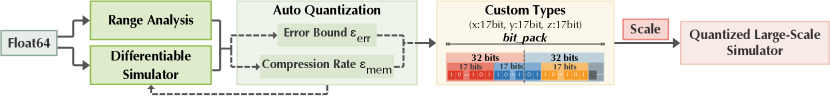
Figure 2. Overview of our method. A differentiable simulator is developed on a relatively low resolution in a generic workflow. The user specifies an evaluation function and launches the simulation with float64. Ranges and derivatives are recorded during this run. Our auto-quantization system can then derive a quantization scheme according to the user’s specification on either error or memory constraints. The user starts to refine the simulation on a higher resolution with the derived quantization scheme before eventually getting a quantized large-scale simulator.

Our method is implemented as an extension to the Taichi programming language (Hu et al., 2019a) to take advantage of its feature of automatic differentiation. However, other automatic differentiable programming frameworks, such as Jax and Tensorflow, can also be adopted to implement differentiable simulations. Therefore, our method can be integrated into these frameworks to obtain quantization schemes as well. See Fig. 2 for an overview of our system.

2. Related Work

High-resolution simulation

QuanTaichi (Hu et al., 2021) introduces quantized data types into the area of physics-based simulations. Empowered by bit-level compression, rich details can be achieved in the simulation results. Besides, sparse data structures (Setaluri et al., 2014; Wu et al., 2018; Museth, 2013; Hu et al., 2019a) are also important to implement high-resolution simulations. These techniques aim to allocate memory only when necessary.

However, if all memory is occupied, it is more sensible to use different resolutions/scales in the simulation scenes (Solenthaler and Gross, 2011; Wang et al., 2018). It is also shown that great visual details can be revealed by adapting the resolution dynamically (Aanjaneya et al., 2017; Ferstl et al., 2014; De Goes et al., 2015). Coarsening the interior elements is a commonly used method. Besides, the Boundary Element Method (BEM) (James and Pai, 1999) is another practical way to enhance the details of simulation (Keeler and Bridson, 2015; Hahn and Wojtan, 2015; Huang et al., 2021). For all methods above, parallelization on multi-GPUs is essential to increasing the upper bound of the simulation scale (Gao et al., 2018; Wang et al., 2020; Wu et al., 2015; Liu et al., 2016). Most of these methods need tailored implementation of the corresponding algorithms, while our method allows users to reduce memory consumption easily with minor modification of the original simulator.

Word-length optimization

In Digital Signal Processing (DSP), word-length optimization (WLO) (Catthoor et al., 1988; Sung and Kum, 1995; Constantinides et al., 2001) is a methodology to determine the quantization schemes of data to trade-off between precision and computational cost on resource-limited devices. The key component of WLO is an evaluation method that approximates the relationship between the quantization errors and the system precision. Early research uses simulation-based methods (Sung and Kum, 1995) to evaluate a set of quantization schemes, which becomes intolerable as the scale and number of variables increase. (Constantinides et al., 2001) uses transfer functions of linear time-invariant (LTI) systems to estimate the system errors. Perturbation analysis is introduced to obtain the error model for non-linear systems, in which the main idea is to consider the quantization error as a small perturbation to the signal and to measure the contribution of each quantization operation to the systematic error. (Shi and Brodersen, 2004) fits an error model by reducing the word length and catching the variation of the total error. (Constantinides, 2006) performs a Taylor expansion and uses the first-order derivatives as the coefficients of the linear combination. Another method of constructing the error model is Interval Arithmetic (IA) (Moore and Yang, 1996). IA is a widely-used method for precision analysis. In IA, numbers are represented not only by themselves but also by a lower and an upper bound. An entire set of arithmetic rules is defined to support the range and error analysis. Typical improvement on IA is Affine Arithmetics (AA), which takes the correlations of signals into consideration (Lee et al., 2006; Vakili et al., 2013).

The main form of WLO is to minimize the hardware cost of the whole system under constraints of the total errors. Because the quantization schemes are represented by integers, solving the optimization is not an easy task. There are two practical ways to solve the optimization. One is to adopt stochastic search methods such as simulated annealing (Constantinides, 2003). The other methodology is setting the fraction bits to the maximum (e.g., 32) at first and then gradually reducing them to find the minimal feasible word length (Shi and Brodersen, 2004).

The intrinsic nature of these DSP tasks indicates that they can yield reasonable results within a short period of time. However, for high-resolution physics-based simulation, fitting the error model by running the simulation multiple times or solving the optimizations by a stochastic search method can be time-consuming.

Differentiable simulations

Running a differentiable simulation is an upstream task for our core algorithm of automatic quantization. Recently, several types of differentiable-simulation methods have been developed. ChainQueen (Hu et al., 2019b) presents a differentiable soft body simulator using the Material Point Method (MPM) with explicit time integration. A differentiable finite element method (FEM) with implicit time integration has also been proposed under the framework of projective dynamics (Du et al., 2021; Bouaziz et al., 2014). Another line of methods approximates the simulation process via neural networks (Battaglia et al., 2016; Li et al., 2019; Sanchez-Gonzalez et al., 2020), which inherits the differentiability from the network. However, the differentiation is not rigorously built on physics, and the physical correctness might not be guaranteed in this way (Du et al., 2021; Bangaru et al., 2021). In addition, Automatic differentiation tools are used to reduce the implementation efforts of differentiable simulations (de Avila Belbute-Peres et al., 2018; Degrave et al., 2019). For instance, DiffTaichi (Hu et al., 2020) proposes a programming framework that automatically generates gradient computation kernels that can be applied to implement various simulation algorithms. As for optimal control tasks, the adjoint method is often utilized to compute the gradients of a loss function with respect to simulation parameters (Geilinger et al., 2020; McNamara et al., 2004). To simplify the programming process and facilitate integration with the compiler, we choose to extend the DiffTaichi framework in our implementation.

Prior to our work, applications of differentiable simulation include parameter estimation, inverse dynamics, and motion control (Liang et al., 2019; Qiao et al., 2020). Our work identifies its significance as the sensitivity of the target function to errors in each input variable and utilizes it as the key ingredient in error estimation.

Dithering

In our framework, we leverage dithering as a method to modulate the distribution of quantization errors. Dithering refers to imposing a random noise on the continuous signal before quantization. It has long been applied in improving the subjective quality of quantized representation for images or speeches (Jayant and Noll, 1990). Schuchman (1964) develops the theory about the property of dithering and proves that a desirable dither signal should generate quantization errors independent of the input signal. The common applications use the manner of subtractive dithering, which enjoys strong mathematical robustness, and is considered to be an efficient algorithm to send a real number using only one bit. Subtractive dithering assumes that the receiver is informed of the random noise, which is subtracted out when reproducing the original signal. However, difficulty in fulfilling this assumption has led to research on non-subtractive dithering with similar effects on the moments of quantization error (Wannamaker et al., 2000). We follow the non-subtractive approach in our implementation since bookkeeping the dithering signal violates our motivation to reduce memory consumption in the first place.

3. Background

3.1. Quantization Procedure for Physics-Based Simulation

Our algorithm returns a quantization scheme of a simulation task, given a memory budget or an accuracy expectation specified by the user. Since a physical simulation proceeds one time step after another, this process is inherently sequential. The error induced by quantized computation accumulates along the simulation procedure. Table 1 summarizes the notations used in our algorithm for clarity.

Table 1. List of notations.

Symbol	Type	Meaning or Definition
$\mathscr{F}$	function	simulation function of one time step
$\mathbf{s}$	vector	system state
$\widetilde{\mathscr{F}}$	function	quantized simulation function
$\widetilde{\mathbf{s}}$	vector	quantized system state
$\mathbf{q}$	vector	component of $\mathbf{s}$
$\mathbf{e}$	vector	error vector
$\mathscr{Z}$	function	evaluation function
$z$	scalar	value of the evaluation function
$x$	scalar	arbitrary variable with quantized type
$\triangle$	scalar	quantization resolution
$b$	scalar	fraction bits for fixed-point numbers
$R$	scalar	range of the fixed-point numbers
$H$	scalar	number of quantized data types
$P$	scalar	number of variables
$T$	scalar	total simulation steps
$N$	scalar	total quantization times
$\phi$	function	quantization encoding function
$\phi^{-1}$	function	quantization dencoding function
$\sigma$	scalar	standard deviation
$\epsilon_{err}$	scalar	target simulation error tolerance
$\epsilon_{mem}$	scalar	target memory compression rate
$M$	scalar	reference memory consumption
$\mathscr{P}$	function	probability density function
$\mathscr{G}$	function	adjoint kernel for computing gradients
$\mathbf{g}$	vector	accumulated squared gradients

Let $\mathscr{F}$ denote a generic simulation function of one time step, which maps the system configuration from the previous time step $\mathbf{s}_{t-1}$ to the current step $\mathbf{s}_{t}$, i.e., $\mathbf{s}_{t}=\mathscr{F}(\mathbf{s}_{t-1})$. Meanwhile, we have a quantized simulation function, $\widetilde{\mathscr{F}}$, which limits the total bit length of $\mathbf{s}_{t}$ and results in a quantized simulation result $\widetilde{\mathbf{s}}_{t}$. $\widetilde{\mathscr{F}}$ can also be understood as imposing a quantization error $\mathbf{e}_{t}$ to the full-precision simulation $\mathbf{s}_{t}$ by eliminating nonzero quantities at its least significant digits. If $\mathbf{s}_{t-1}$ is quantized, we have:

(1) $$\widetilde{\mathbf{s}}_{t}=\widetilde{\mathscr{F}}(\widetilde{\mathbf{s}}_{t-1})=\mathscr{F}(\widetilde{\mathbf{s}}_{t-1})+\mathbf{e}_{t}.$$

During the simulation, $\mathbf{s}$ is composed of several generalized coordinates and other attributes, e.g., particle positions, velocities etc: $\mathbf{s}=(\mathbf{q}_{1}^{T},\mathbf{q}_{2}^{T},\cdots,\mathbf{q}_{H}^{T})^{T}$, where $H$ is the number of different physical quantities, such as components of position and velocity involved in the simulation, and each generalized coordinate $\mathbf{q}_{i}$ is of $P_{i}$ dimension. For example, in material point method (MPM), $P_{i}$ can be the number of particles or grid cells (see Fig. 3).

We assume that the user appoints a specific evaluation function, $\mathscr{Z}$, which measures a metric of interest of the simulation over $T$ time steps. Naturally, the goal of an automatic quantizer seeks to minimize $\delta z$, the difference between the evaluation function values of the quantized and full-precision simulations:

(2) $$\delta z=\left|\mathscr{Z}\big{(}\widetilde{\mathbf{s}}_{0},\widetilde{\mathbf{s}}_{1},\cdots,\widetilde{\mathbf{s}}_{T}\big{)}-\mathscr{Z}\big{(}\mathbf{s}_{0},\mathbf{s}_{1},\cdots,\mathbf{s}_{T}\big{)}\right|^{2}.$$

For example, $\mathscr{Z}$ can be set to calculate the kinetic energy of all the particles in a fluid simulation, and then $\delta z$ should identify the magnitude of the numerical viscosity induced by the quantization.

Figure 3. Notations of a quantized MPM simulation. In this case, we only quantize the attributes stored on particles, so there are $P$ variables for each attribute, where $P$ is the number of particles.

We follow the same quantization algorithm as in (Hu et al., 2021). A quantized type variable is stored in the memory with a limited digit count but decoded as a standard float32 or float64 quantity when participating in the computation. Typically, this operation is lossless. The reverse operation i.e., the encoding from a regular float to the quantized type, however, brings a quantization error.

Consider a quantization operation of a fixed-point transformation $\phi:\mathbb{R}\mapsto\mathbb{Z}$, which takes a scalar $v\in\mathbb{R}$ as the input and produces its integer representation $u\in\mathbb{Z}$ and its inverse $\phi^{-1}$, estimating the floating-point value from a quantized integer $u$:

(3) $$u=\phi(v)=\lceil v/\triangle\rfloor,\quad\phi^{-1}(u)=u\cdot\triangle,$$

where $\lceil\cdot\rfloor$ is the function of rounding to the nearest integer and $\triangle=2^{-b}R$ is the resolution of the corresponding quantization, where $b$ and $R$ are the fraction bits and the range for $v$ respectively. The error induced by $h$ then becomes $e=v-\phi^{-1}\big{(}\phi(v)\big{)}$.

In this quantized simulation procedure, we need to determine the optimal value for fraction bits $b$ and ranges $R$ for each custom type. For example, in a 3D Eulerian fluid simulation, each cell is associated with a vector of velocity ($\mathbf{v}$) and a scalar of pressure ($p$). If we want to take advantage of quantized simulation, we need to figure out how many fraction bits we should assign to each quantity and what is the feasible range. However, there are many choices for the fraction bits, i.e., 16 bits for $p$ and each component of $\mathbf{v}$ or 10 bits for $p$ and $3\times 18$ bits for $\mathbf{v}$. Different choices will lead to different simulation errors and memory compression rates. In this paper, we focus on how to automatically obtain the number of fraction bits according to users’ requirements on memory budget or computation precision. As for the range analysis, we record the ranges from the full precision simulation and multiply the ranges by a factor (e.g., 2) to prevent overflowing.

3.2. Uncertainty Propagation Theory

Considering the quantization operation as imposing an error $e_{i}$ to a variable $x_{i}$, we can model the relationship between the quantity $\delta z$ and system configuration variables using uncertainty propagation theory (Cohen, 1998). This theory proposes to measure the uncertainty of a variable as standard deviation and construct a step-by-step propagation procedure to estimate the final uncertainty of a composite function. Specifically, if all the input variables are uncorrelated, the uncertainty of a synthesized variable $z$ can be estimated from the uncertainty of all its contributing variables $\{x_{i}\}$ as follows:

(4) $$\sigma_{z}^{2}=\sum_{i=1}\left(\frac{\partial z}{\partial x_{i}}\right)^{2}\sigma_{x_{i}}^{2},$$

where $\sigma_{z}^{2}$ and $\sigma_{x_{i}}^{2}$ are the variances of $z$ and $x_{i}$, respectively.

In our case, Eq. (4) allows us to track the uncertainty from all the quantization errors for $\delta z$ in Eq. (2):

(5) $$E[\delta z]=\sum_{i=1}^{N}\int_{-\triangle_{i}/2}^{\triangle_{i}/2}\left(\frac{\partial\mathscr{Z}}{\partial e_{i}}\right)^{2}e_{i}^{2}\mathscr{P}(e_{i})\mathrm{d}e_{i}$$

where the summation traverses all the components in each generalized coordinate across $T$ time steps, and thus $N=\sum_{i=1}^{H}P_{i}\cdot T$. The integral range is the absolute error bound, which is half of the quantization resolution. The probability density function for an error component $e_{i}$ is denoted as $\mathscr{P}(e_{i})$.

Note that we assume that the quantization errors are uncorrelated, and therefore the cross terms of correlations are neglected in Eq. (4) Under this assumption, our model lacks the ability to recognize the correlation between quantization errors. It is essentially a localized linear expansion at the point of the true value. Hence, we introduce dithering operations so that this form of uncertainty propagation can be applied to our problem properly (see Sec. 5).

In our implementation, a full-precision simulation needs to be carried out first to obtain $z=\mathscr{Z}(\bm{s}_{i})$, the partial derivatives of the quantization error, as well as the range of each custom data type.

4. Uncertainty-Propagation-based Quantization

In this section, we first describe the details of the objective functions and then present how to convert the automatic quantization problem into a continuous optimization problem using vector variables consisting of the quantization resolution $\triangle$ of each quantity.

4.1. Formulation of Objective Functions

The proposed automatic quantization includes two different strategies, aiming to provide the user with either a controllable accuracy bound or a guaranteed memory compression rate. Below we elaborate the objective functions for these two strategies in detail.

Error-bounded quantization.

Being quantized, simulation variables inevitably lose precision under capped bit length, which potentially impacts the simulation quality and may even result in visible artifacts. Error-bounded quantization scheme aims to address this concern. It offers the accuracy guarantee prescribed by a user-specified error bound and lowers the total memory consumption:

(6) $$\min_{b_{h}}\sum_{h=1}^{H}P_{h}b_{h},\quad\text{s.t.}\;E[\delta z]<(\epsilon_{err}\cdot z)^{2},$$

where $P_{i}b_{i}$ gives the memory footprint of each generalized coordinate $\mathbf{q}_{i}$, $E[\cdot]$ computes the expectation of a random variable, $z=\mathscr{Z}\big{(}\mathbf{s}_{0},\mathbf{s}_{1},\cdots,\mathbf{s}_{T}\big{)}$ is the reference simulation metric obtained without quantization, and $\epsilon_{err}$ is the relative error tolerance specified by users.

Memory-bounded quantization.

In a different scenario where the hardware resource is limited, a guaranteed memory consumption could be more favored in practice. To this end, we pose the memory compression rate as a hard constraint that must be fulfilled by the automatic quantization algorithm. Based on this constraint, we push to suppress the accuracy loss as much as possible:

(7) $$\min E[\delta z]\quad\text{s.t.}\sum_{h=1}^{H}P_{h}b_{h}<\epsilon_{mem}\cdot M,$$

where $\epsilon_{mem}$ is the memory compression rate specified by the user, $M$ stands for the total memory usage for the full-precision simulation, e.g., ${M=\textsf{sizeof}(\leavevmode\lstinline{{\lst@@@set@language\lst@@@set@numbers\lst@@@set@frame\lst@@@set@rulecolor\lst@@@set@language\lst@@@set@frame\footnotesize{\@listingGroup{ltx_lst_identifier}{float32}}}}})\sum P_{h}$, assuming float32 is used as the data type.

4.2. Continuous Optimization Problem

We change the fraction bit variable $b_{h}$ into its corresponding quantization resolution variable $\triangle_{h}$ for objective functions defined in Sec. 4.1, such that the automatic quantization problem can be solved in a continuous way. Assuming $\mathscr{P}(e_{i})$ follows a uniform distribution, Eq. (5) is integrated into:

(8) $$E[\delta z]=\frac{1}{12}\sum_{h=1}^{H}\triangle_{h}^{2}g_{h}\overset{\operatorname{def}}{=}\frac{1}{12}\sum_{h=1}^{H}\triangle_{h}^{2}\left(\sum_{t=0}^{T}{\sum_{i=1}^{P_{h}}\left(\frac{\partial z}{\partial x_{t,h}^{i}}\right)^{2}}\right),$$

where the coefficient $g_{h}$ is the accumulated squared gradient of the variable with type $h$. More, specifically, since $b_{h}=-\log_{2}{\frac{\triangle_{h}}{R_{h}}}$, the objective function in Eq. (6) after the variable quantization is as follows:

(9) $$\min_{\triangle_{h}}\sum_{i=1}^{H}{-P_{h}\log_{2}{\frac{\triangle_{h}}{R_{h}}}}$$

$$s.t.\frac{1}{12}\sum_{h=1}^{H}{\triangle_{h}^{2}g_{h}}<(z\epsilon_{err})^{2}$$

$$\triangle_{h}\in\mathbb{R^{+}}$$

Such a continuous optimization problem has an analytical solution using Lagrange multiplier method:

(10) $$\triangle_{h}=\sqrt{\frac{12P_{h}(\epsilon_{err}\cdot z)^{2}}{g_{h}\sum_{h=1}^{H}{P_{h}}}}$$

The fraction bits for each type of variable are then obtained according to the value of $\triangle_{h}$. Likewise, we can obtain the analytical solution for memory-bounded scenario in Eq. (7) after the variable quantization. Please refer to section 4 in supplementary material for the solution derivations.

Discussions.

The objective function in Eq. (9) is a local linearization of Eq. (6). Indeed, the linearization can be iteratively updated at new values of $\triangle_{h}$ after we solve Eq. (9). However, such an iterative algorithm incurs a high computational cost since the gradients must be computed after another round of forwarding simulation in auto-diff. In practice, we have found linearizing using the gradients computed with full-precision simulation is able to produce approximate solutions that have the desirable properties: the quantized simulation result is visually consistent with the full-precision simulation, and their differences from the full-precision simulation or the memory footprint can be controlled in most cases using our objective functions with dithering. Therefore, we accept the solution without iteration, which means we prefer speed over optimality in automatic quantization. It can provide users with faster feedback. The pseudocode of solving the quantization scheme under error-bound constraints can be found in Algorithm 1.

Input: $\epsilon_{err}$

Output: $(b_{1},R_{1}),...,(b_{H},R_{H})$

1 $T\leftarrow$ Total simulation steps

2 $H\leftarrow$ Number of quantized data types

3 for h = 1 to H do

4       $P_{h}\leftarrow$ number of variables using type $h$  

5 end for

6$\mathbf{s}_{0}\leftarrow$ Initial conditions

7 for t = 0 to T-1 do

       // step forward

8        $\mathbf{s}_{t+1}\leftarrow\mathscr{F}(\mathbf{s}_{t})$

       // update ranges for each quantity

9        Update $R_{1}...R_{H}$ according to $\mathbf{s}_{t+1}$

10 end for

// compute the evaluation function

11  $z\leftarrow\mathscr{Z}\big{(}\mathbf{s}_{0},\mathbf{s}_{1},\cdots,\mathbf{s}_{T}\big{)}$

12 Back propagation and accumulate gradients in g according to Eq. (8)

13 for h = 1 to H do

14       $\triangle_{h}\leftarrow\sqrt{\frac{12P_{h}(\epsilon_{err}\cdot z)^{2}}{g_{h}\sum_{h=1}^{H}{P_{h}}}}$

15       $b_{h}\leftarrow\lceil-\log_{2}\frac{\triangle_{h}}{R_{h}}\rceil$

16 end for

ALGORITHM 1 Automatic quantization scheme based on an error-bound constraint.

5. Dithering

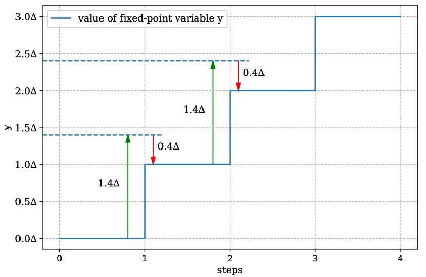
Figure 4. An illustration of the dependence between quantization errors. At each frame, the variable $y$ is added by $1.4\triangle$ (see the green arrows) and then $y$ is rounded down causing a quantization error of $-0.4\triangle$ (the red arrows). In this simulation pattern, the quantization errors for each frame are all equal to the previous one. Therefore, assuming they are independent random variables is not always reasonable.

So far, we model the quantization error as random uniform distribution for each quantization operation, and we assume they are independent in the simulation. However, it is not a realistic assumption in general settings. The quantization error is directly coupled with the digit after the least significant bit. It is liable to reflect the functional relationship between the state variables. In other words, if the uncorrelated assumption on the quantization error $Cov(e_{t_{1},i_{1}},e_{t_{2},i_{1}})=0$ does not hold for every distinct pair of $(t_{1},i_{1})\neq(t_{2},i_{2})$, it is not safe to apply Eq. (4), since the actual error can be much bigger than the estimation.

As an example, assuming we have a variable $y$ represented by a two-bit unsigned fixed-point number with four quantization levels. Starting from $y=0$, we add $1.4\triangle$ to $y$ for each time step. In this pattern, the quantization error of the first step is $-0.4\triangle$, which leads to the subsequent quantization errors being all $-0.4\triangle$. Therefore we cannot assume the quantization errors are independent random variables in this case. Please see Fig. 4 for details.

As shown in (Hejn and Pacut, 1996; Gray, 1990; Widrow, 1961), dithering is an effective solution to supply the necessary condition of modeling the quantization error as uniform and uncorrelated. Overall, we follow the practice of non-subtractive dithering (Wannamaker et al., 2000) in our system. To elaborate, in each store operation, we impose an additive uniform noise before rounding:

(11) $$u=\theta_{dither}(v)=\lfloor\frac{v}{\triangle}+\xi\rceil,\quad\xi\sim U(-\frac{1}{2},\frac{1}{2})$$

This dithered representation is a more accurate description than a deterministic round-to-nearest scheme because it has an unbiased first moment. Even with unevenly distributed signals, dithered quantization presents a stronger tolerance and leads to a less biased result. Specifically, if we denote the normalized round-off error, i.e. $\frac{v}{\triangle}-\lfloor\frac{v}{\triangle}\rfloor$, as $Y\in[0,1)$, the probability of performing a round-up is exactly $Y$, i.e. $\mathscr{P}(Y+\xi>0.5)=Y$. In other words, the dithered value after rounding shares the same expectation of $Y$ regardless of the distribution of $Y$. In comparison, if $Y$ distributes unevenly between the two intervals $[0,0.5),[0.5,1)$, a naive rounding scheme will result in a bias in the expectancy. However, the error variance still depends on the value of $Y$ and the $\frac{1}{12}\triangle^{2}$ variance of quantization error remains an unsubstantiated assumption. In practice, our dithering scheme works better than an alternative implementation without dithered quantization (see Fig. 5 for an example).

Figure 5. Effect of our dithering scheme. Top: quantized simulation without dithering where the letters fall with different vertical velocities. Bottom: quantized simulation with our dither scheme where the letters align neatly.

6. Gradient Computation

Our method relies on the gradient of each variable involved in the estimation of the system error in Eq. (8). We thus adopt the differentiable programming framework of DiffTaichi (Hu et al., 2020) and adhere to its restrictions to compute the gradients. However, DiffTaichi requires storing the states of each frame for back-propagation. This requirement leads to linear growth of memory footprint, which restricts the steps of the simulation. Thus, we follow the bisection algorithm (Griewank, 1992) to achieve logarithmic spatial complexity w.r.t the growth of simulation steps.

With auto-diff implementation, gradient $\frac{\partial z}{\partial\mathbf{s}_{t}}$ is calculated from the chain rule below:

(12) $$\frac{\partial z}{\partial\mathbf{s}_{t}}=\frac{\partial z}{\partial\mathbf{s}_{t+1}}\frac{\partial\mathbf{s}_{t+1}}{\partial\mathbf{s}_{t}}$$

where $\frac{\partial z}{\partial\mathbf{s}_{t+1}}$ is the result from last step which is carried backward, and $\frac{\partial\mathbf{s}_{t+1}}{\partial\mathbf{s}_{t}}$ is a function of $\mathbf{s}_{t}$. In all, the compiler transforms the forward program $\mathbf{s}_{t+1}=\mathscr{F}(\mathbf{s}_{t})$ to the adjoint kernel $\mathscr{G}$ which calculates $\frac{\partial z}{\partial\mathbf{s}_{t}}$ from input $\mathbf{s}_{t}$ and $\frac{\partial z}{\partial\mathbf{s}_{t+1}}$:

(13) $$\frac{\partial z}{\partial\mathbf{s}_{t}}=\mathscr{G}(\mathbf{s}_{t},\frac{\partial z}{\partial\mathbf{s}_{t+1}})$$

Therefore, we must recover state $\mathbf{s}_{t}$ before execution of adjoint kernel before back-propagating the gradients from $\mathbf{s}_{t+1}$ to $\mathbf{s}_{t}$. In the implementation of ChainQueen, all the states $\mathbf{s}_{0},\dots,\mathbf{s}_{T}$ are stored in pre-allocated areas so that they can be referenced out of the box (Hu et al., 2019b).

Our bisection algorithm is similar to DiffTaichi’s checkpointing method. Each checkpoint stores the entire time section so that a rerun is possible. Trading time for space is possible by not keeping all the states at hand but only recovering them by restarting from the nearest checkpoint when necessary. However, instead of dividing the simulation into uniform segments as suggested by DiffTaichi, we allocate the checkpoints unevenly so that each checkpoint is in the middle of the last checkpoint and the current state.

In practice, we organize the states $\mathbf{s}_{0},\dots,\mathbf{s}_{T}$ in a binary B+ tree, with storage only on its leaves. The leaf nodes are indexed by $0,\dots,T$ from left to right, corresponding to the states $\mathbf{s}_{0},\dots,\mathbf{s}_{T}$. Each non-leaf node serves as a signpost, which records the smallest value of their sub-trees. We equate the checkpoints to the non-leaf nodes according to the value, i.e., a non-leaf node with a signpost value $t$ corresponds to a checkpoint storing the information of state $\mathbf{s}_{t}$. In a time step $t$, only the checkpoints on the path from the root to leaf node $t$ reside in memory. Upon execution of the routine $\frac{\partial z}{\partial\mathbf{s}_{t}}=\mathscr{G}(\mathbf{s}_{t},\frac{\partial z}{\partial\mathbf{s}_{t+1}})$ to back-propagate gradients from step $(t+1)$ to $t$, state $\mathbf{s}_{t}$ is required as an input. With the above structure, we trace back to the nearest common ancestor of $\mathbf{s}_{t}$ and $\mathbf{s}_{t+1}$ where we will find the nearest checkpoint available and then execute a rerun from there. (Please refer to Fig. 6 for an illustration.)

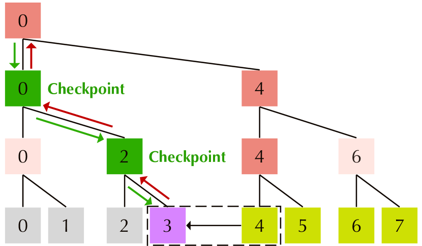
Figure 6. Illustration of the bisection algorithm. Adjoint kernel is back propagating $\frac{\partial z}{\partial\mathbf{s}_{4}}$ to $\frac{\partial z}{\partial\mathbf{s}_{3}}$. The states at steps 0,4 are stored as checkpoints (shown in red). To recover $\mathbf{s}_{3}$, retrace to the nearest non-empty checkpoint (red arrow), which is state $\mathbf{s}_{0}$, the nearest common ancestor of leaf node of state $\mathbf{s}_{3}$ and $\mathbf{s}_{4}$. A rerun is then executed from $\mathbf{s}_{0}$. During the rerun process, the checkpoints at depth 1 and 2 (with root at depth 0) are updated after 0 and 2 steps respectively (green arrow, new checkpoints shown in green).

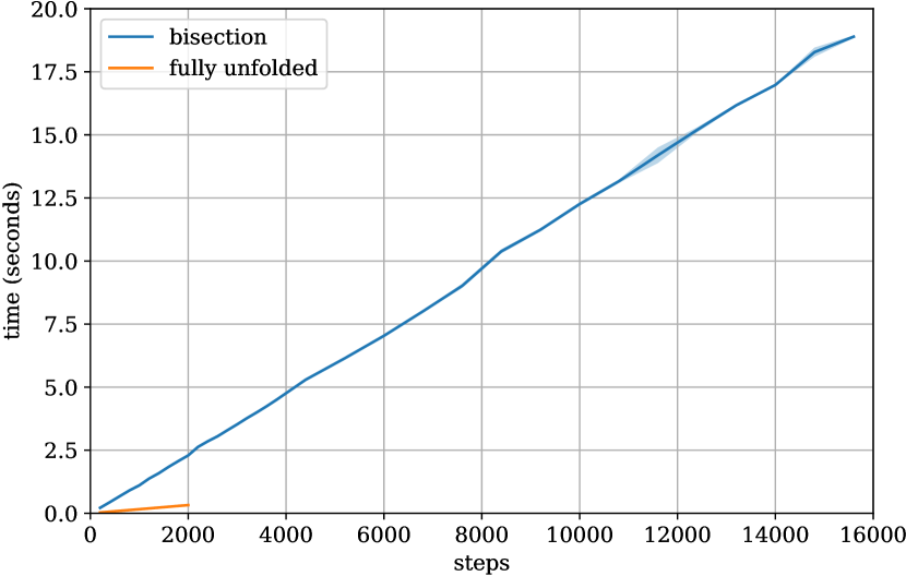
Figure 14. Comparison of temporal complexity between the bisection algorithm (blue) and the fully unfolded scheme (orange). Note that the orange line ends after 2000 steps since GPU fails to allocate enough memory, and the bisection algorithm is roughly 8 times slower under this situation. However, the bisection scheme is nearly free from memory limitations.

Overall, this bisection algorithm achieves temporal and spatial complexity of $O(N\log N)$ and $O(\log N)$, respectively, as opposed to $O(N)$ and $O(\sqrt{N})$ of DiffTaichi, and thus significantly expanding the capacity of total number of steps in a memory-bound scenario. The actual running time is reported in Fig. 14.

7. Bit Pack Data Structure

After solving the optimization problem defined in Eq. (6) or Eq. (7), we need to place the custom-length data types into the memory automatically. Therefore, we propose a new bit-level data structure, namely bit pack, which allows us to easily place arbitrary length custom data types into memory without worrying about the bit-level layout. Similar to the bit-level container bit struct proposed by (Hu et al., 2021), bit pack is also a tree-based custom data type container. However, bit struct only supports hardware-native data types as the variable containers, which makes users restrained when working with custom data types. There are two main limitations of bit struct. First, users have to modify the code describing the placements of quantized data types if the number of bits inside the bit struct exceeds the maximum length of the physical type. The following code snippet is an example. The code describes the memory usage of a particle in a 3D MPM simulation, where $\mathbf{p}$, $\mathbf{v}$, and $\mathbf{F}$ represent the position, velocity, and deformation gradient of the particle, respectively.

⬇

# using bit struct

ti.root.bit_struct(num=64).place(p(0), p(1), p(2))

ti.root.bit_struct(num=64).place(v(0), v(1), v(2))

ti.root.bit_struct(num=64).place(F(0, 0), F(0, 1), F(0, 2), F(1, 0))

ti.root.bit_struct(num=64).place(F(1, 1), F(1, 2), F(2, 0), F(2, 1))

ti.root.bit_struct(num=32).place(F(2, 2))

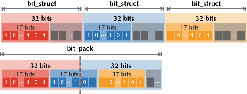
Figure 7. Comparison of bit pack with bit struct. Two 17-bit numbers do not fit into a single 32-bit bit struct, and the three 17-bit elements consume three bit structs. In contrast, the three elements can be contained by two 32-bit bit packs.

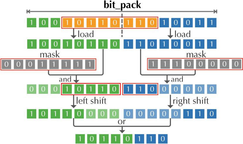
Figure 8. Illustration of the load operation on a custom type variable spanning two different physical words based on our bit pack data structure. We first load the two words, then use a series of bit operations to reconstruct the original data.

In the example above, the total bit width of $\mathbf{p}$ cannot exceed 64. However, this constraint cannot be guaranteed before the quantization scheme is derived from our optimization. Users may need to re-organize the placement, for instance, move the last component of $\mathbf{p}$ into another bit struct if the bit width violates the limit. Besides, when designing a quantized simulator manually, trial and error takes the most of the time. Frequently adjusting the placement by modifying codes can be troublesome.

The second limitation of bit struct is that it does not allow custom data types to span across two physical words. See Fig. 7 for an example. Supposing we have three 17-bit custom integers to be placed in 32-bit bit structs. Due to the limitation, we have to use $3\times 32$ bits to accommodate them, leading to $3\times 15$ bits unfilled.

We propose bit pack to address this problem using a simple strategy. Custom data types can be placed into the memory contiguously, and the compiler will detect the case that the data types span across two physical words. When a data type is split by physical words, the compiler will generate code performing a series of bit operations to reconstruct the custom data types. See Fig. 8 for a visual demonstration. With the help of bit pack, the above example only requires one line of code to describe the memory placement clearly as below, and no more code changes in other parts are needed.

⬇

# using bit pack

ti.root.bit_pack().place(p, v, F)

8. Experiments and Evaluations

We conduct experiments to evaluate the effectiveness, performance, and scalability of our method. We further develop three large-scale simulators with our workflow. Implementation details of all the quantization schemes presented in this section can be found in the supplemental materials.

8.1. Effectiveness

We evaluate the controllability of our approach in both error-bounded and memory-bounded scenarios using three 2D simulators, including an MLS-MPM (Hu et al., 2018) elastic body simulator, an MLS-MPM fluid simulator, and an advection-reflection (Zehnder et al., 2018) Eulerian smoke simulator.

Error-bounded quantization

To evaluate the capability of the error-bounded quantization, we conduct experiments of 2D elastic body and Eulerian fluid simulation on an NVIDIA GTX 1080Ti GPU with 11 GB memory.

We simulate eight elastic squares falling down and colliding with each other based on the MLS-MPM algorithm (Hu et al., 2018). Particles are the primary memory consumer, while background grids use less memory due to sparsity. We store positions ($\mathbf{p}$), velocities ($\mathbf{v}$), deformation gradients ($\mathbf{F}$) and affine velocity field ($\mathbf{C}$) on each particle which add up to $48$ bytes with IEEE754 single floating-point precision. The MPM experiment is conducted with $80,000$ particles and $128\times 128$ background grids. We use the kinetic energy in the final state as the evaluation function. The entire simulation process includes 8192 steps with a time interval of $2\times 10^{-4}$.

Our 2D Eulerian Smoke experiment is conducted using a differentiable advection-reflection (Zehnder et al., 2018) solver. We perform advection in a semi-Lagrangian scheme with RK-3 path integration. We solve Poisson’s equation using $64$ Jacobian iterations. The grid resolution and time interval are $256\times 256$ and $0.01$, respectively. The evaluation function is set to be the squared sum of smoke density on all grids in the final state. Finally, the quantized variables are the pressure and velocity of the grids.

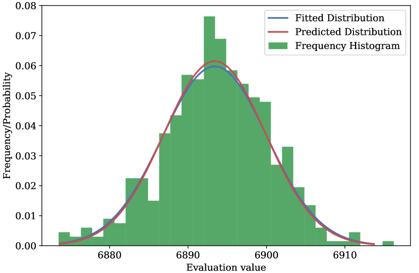
Figure 9. Distribution of the evaluation function on quantized MPM elastic body simulation. The probability density function fitted from the mean and variance of the observed samples is shown in blue. The red curve representing the predicted density function is computed through Eq. (8) with the gradients of the simulation and the testing quantization resolution. The close match between the two curves validates our error estimation model.

In our experiments, we consider the evaluation function of a quantized simulation as a normal distribution. To validate this assumption, we first run a quantized 2D MPM elastic body simulation 500 times and record the frequency of the function. The histogram of the distribution is shown in Fig. 9, from which we can see the values of the evaluation function can be well approximated using a normal distribution. Please refer to the 4th column of Table 1 in our supplementary materials for the quantization scheme used in this experiment.

We set the relative error tolerance $\epsilon_{err}$ to four different magnitudes: $10^{-1}$, $10^{-2}$, $10^{-3}$, and $10^{-4}$. The quantized simulation is executed 20 times for each magnitude, where the mean and standard deviations are recorded as $\mu_{sim},\sigma_{sim}$. Since we model the evaluation function as a normal distribution, we consider the error is successfully under control if the evaluation function value of a quantized simulation falls in a range of $3\epsilon_{err}$ centered at $\mu_{sim}$. We record the number of successful controls out of 20 tests as the success rate.

From Table 2 we can see that as the error tolerance increases, the number of quantization bits increases, and the fluctuation of the evaluation function becomes smaller. The bias and variance satisfy well with the error tolerance in most cases. The failure case of Eulerian smoke in the second row of Table 2 is quantized with only 4 fraction bits on pressure and 6 fraction bits on velocity. This shows the potential hazard of abuse, where a radical setting of the error bound might lead to a bold quantization scheme and a large deviation from the full-precision simulation. In this situation, the local linearization cannot approximate Eq. (5) well enough.

As mentioned above, our method can be solved iteratively, but we only adopt the solution without iteration for lower computational costs. To validate this design choice, we solve the optimization iteratively in the example of 2D smoke simulation. We find that the optimization process converges after no more than six iterations, and the corresponding result of the iterative approach differs from the non-iterative solution by at most one bit on each variable. However, the iterative solution is highly expensive due to the re-computation of gradients at each iteration, so we keep using the non-iterative solution in the rest of our experiments. Please refer to section 3.1 in the supplementary material for the detailed results.

Table 2. Results of the error-bounded experiments. The MPM elastic body and Eulerian smoke simulations are labeled as Exp. 1 and Exp. 2. The column of $\epsilon_{err}$ is the relative error tolerance used in each experiment. Control Objective in the table dictates the absolute tolerance of the simulation error. We use S.R. and M.C. as abbreviations for success rate and memory compression. The quantized evaluation function lands nicely within the range of permitted error bound. Of all the $160$ experiments, there are $136$ times that our quantization scheme manages to control the value.

Exp.	$\bm{\epsilon_{err}}$	Control Objective	Quantized Evaluation Function	S.R.	M.C.
1	0.1	$6.9\pm 2.1\times 10^{3}$	$7.1\pm 1.1\times 10^{3}$	19/20	$2.00\times$
2	0.1	$1.87\pm 0.56\times 10^{4}$	$3.69\pm 0.08\times 10^{4}$	0/20	$5.05\times$
1	0.01	$6.89\pm 0.21\times 10^{3}$	$6.90\pm 0.06\times 10^{3}$	20/20	$1.67\times$
2	0.01	$1.875\pm 0.056\times 10^{4}$	$1.90\pm 0.04\times 10^{4}$	17/20	$3.20\times$
1	0.001	$6.893\pm 0.021\times 10^{3}$	$6.895\pm 0.008\times 10^{3}$	20/20	$1.42\times$
2	0.001	$1.8749\pm 0.0056\times 10^{4}$	$1.875\pm 0.003\times 10^{4}$	20/20	$2.40\times$
1	0.0001	$6.8934\pm 0.0021\times 10^{3}$	$6.8946\pm 0.0007\times 10^{3}$	20/20	$1.23\times$
2	0.0001	$1.87486\pm 0.00056\times 10^{4}$	$1.87488\pm 0.00019\times 10^{4}$	20/20	$1.96\times$

Memory-bounded quantization.

We evaluate the scenario of memory-bound quantization on a 2D MLS-MPM based fluid simulation of a dam break example. Similar to the previous MPM elastic body simulations in error-bounded experiments, we store $\mathbf{p}$, $\mathbf{v}$, and $\mathbf{C}$ of each particles. As for the deformation gradient $\mathbf{F}$, we follow Tampubolon et al. (2017) to track its determinant $J$ instead of its matrix elements for improved numerical stability. In a full-precision simulation, it takes $36$ bytes to store the attributes of each particle. We use the kinetic energy of the final time step as the evaluation function. We run the simulation with $10,000$ particles and $128\times 128$ background grids. The simulation lasts for 16,384 steps with a time interval of $2\times 10^{-4}s$. The experiments run on an NVIDIA RTX 3090 GPU with 24 GB memory.

We set the control parameters of the target compression rate from 40% to 60% We run the simulation 10 times for each target compression rate and record the mean $\mu_{mem}$ and standard deviation $\sigma_{mem}$. The results can be found in Table 3. Using the compression rate as the quantization target makes it difficult to define a successful error control as in the previous section, because the error bound is used as a soft constraint. So we use an error metric denoted as $e_{mem}=\sqrt{\sigma_{mem}^{2}+(\mu_{mem}-z)^{2}}$, where $z$ is the reference value obtained by full-precision simulation. Given this error metric, even in the case of the highest compression rate ($2.5\times$), the relative error is only $9.9$%. Meanwhile, the visual quality is still comparable to the full-precision version. Please refer to the visual comparison in Fig. 10. In summary, our automatic quantization scheme successfully assigns appropriate numbers of quantization bits to each variable according to their contribution to the overall error under the limited memory budget.

Table 3. Memory-bound experiments. The target compression rate is the control parameter specified by users. The real compression rate is computed according to the quantization scheme derived from our optimization. The reference evaluation function value is $1.32\times 10^{3}$.

Target Compression Rate ($\epsilon_{mem}$)	Real Compression Rate	Evaluation Function
60% ($1.67\times$)	58.3% ($1.71\times$)	$1.28\pm 0.06\times 10^{3}$
50% ($2.0\times$)	47.2% ($2.12\times$)	$1.29\pm 0.08\times 10^{3}$
40% ($2.5\times$)	37.8% ($2.64\times$)	$1.25\pm 0.11\times 10^{3}$

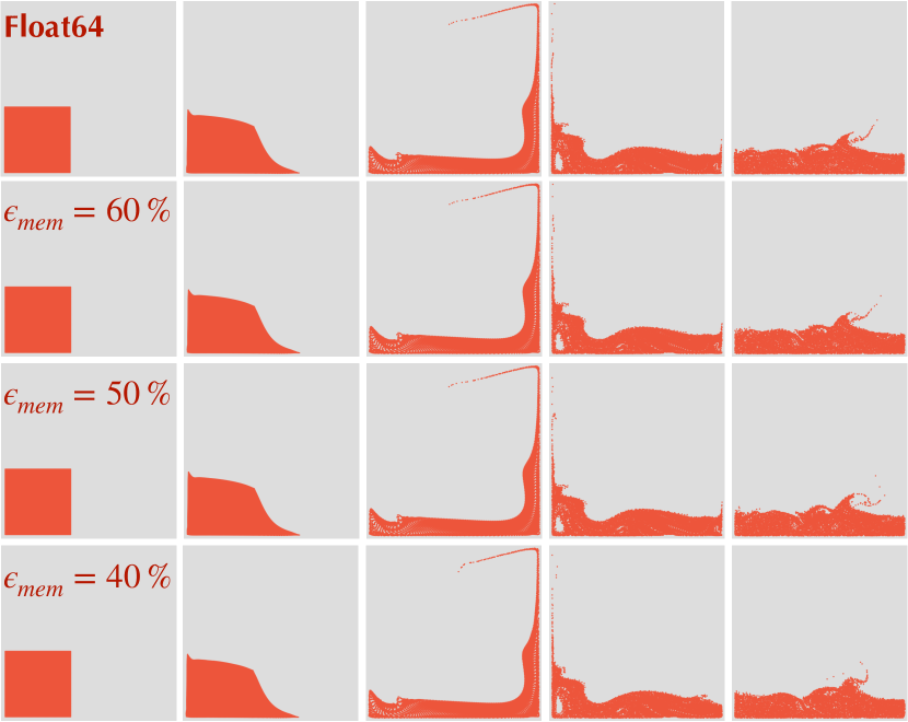
Figure 10. Visual comparison for the memory-bounded experiments.

Table 4. The success rate and evaluation function values for the first two experiments of optimality check. The base quantization scheme with a success rate of (20/20) and evaluation function of ($6.90\pm 0.06\times 10^{3}$) can be found in the supplemental material.

Bits Taken	Success Rate		Evaluation Function
	Reduce All	Reduce Half	Reduce All	Reduce Half
1	19/20	20/20	$6.9\pm 0.1\times 10^{3}$	$6.88\pm 0.09\times 10^{3}$
2	13/20	17/20	$6.9\pm 0.3\times 10^{3}$	$6.8\pm 0.2\times 10^{3}$
3	5/20	12/20	$7.3\pm 0.7\times 10^{3}$	$6.9\pm 0.4\times 10^{3}$

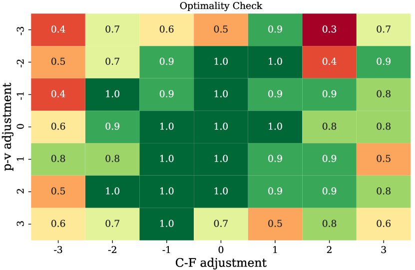
Figure 11. Optimality check. We conduct two orthogonal adjustments: to move bits from $\mathbf{p}$ to $\mathbf{v}$ (positive y-axis and vice versa) and from $\mathbf{C}$ to $\mathbf{F}$ (positive x-axis). The success rate is counted based on ten repetitions on each quantization scheme.

Optimality check

Aided by the accurate prediction of the simulation error, the quantization scheme derived from our system can reach a very close vicinity to the critical point. We verify this claim using the previous MLS-MPM elastic body simulation with the same experiment settings. We first solve the optimization by setting the relative error bound to 0.01 and then make minor adjustments to the quantization scheme in three different ways:

1. Unanimously take away bits in all data types.

2. Randomly reduce the length on half of the data types.

3. Move bits from some data types to others.

The bit reduction results (the first two methods) are recorded in Table 4, and the result of bits-redistribution (the last method) is shown in Fig. 11 and our supplemental materials. In these experiments, the success rates are counted by 20 and 10 repetitions, respectively. This experiment reveals that even with less than 10% modification of our generated scheme, there is a significant impact on the success rate of the error constraints, and our quantization scheme is almost the most memory-efficient scheme that satisfies the error constraints.

Dithering

To showcase the effectiveness of dithering in reducing the overall errors of quantized simulation, we use a quantization scheme with a relatively high memory compression ($2.5\times$). We choose kinetic energy as the evaluation function to measure the errors. Table 5 shows that the dithered simulation leads to a much more accurate evaluation function value in this challenging case, while the simulator exhibits significant deviation from the full-precision float64 simulation without dithering, which is confirmed by the target function value and the visual comparisons in Fig. 12. The explanation for the failure is that the induced round-off errors are ill-distributed, contradicting our assumption of uniform independence distribution in the error model. We record the aggregated ratio of round-ups and round-downs and find that the ratio of rounding up and rounding down is $1.47$ for the $y$ component of velocity, as opposed to the dithered result of $1.00$ (See Table 5).

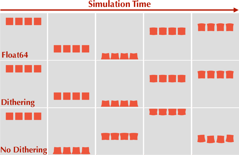
Figure 12. Effect of our dithering scheme. Without dithering (the bottom row), the elastic cubes fall from rest, bounce over the initial position, and smash the ceiling. In comparison, the dithered simulation with the same bit number (the second row) closely resembles the full-precision reference (the first row).

Table 5. The effectiveness of dithering. We compare three data types on a 2D MPM elastic body simulation. The result without dithering deviates far away from the full-precision reference and the case with dithering. Also the uneven ratio of round-ups to round-downs can be observed in the case without dithering.

Data Type	Evaluation Function	Round-ups/ Round-downs
float64	$1.378\times 10^{5}$	-
Quantize with dithering	$1.370\times 10^{5}$	0.999976
Quantize without dithering	$8.885\times 10^{5}$	0.683994

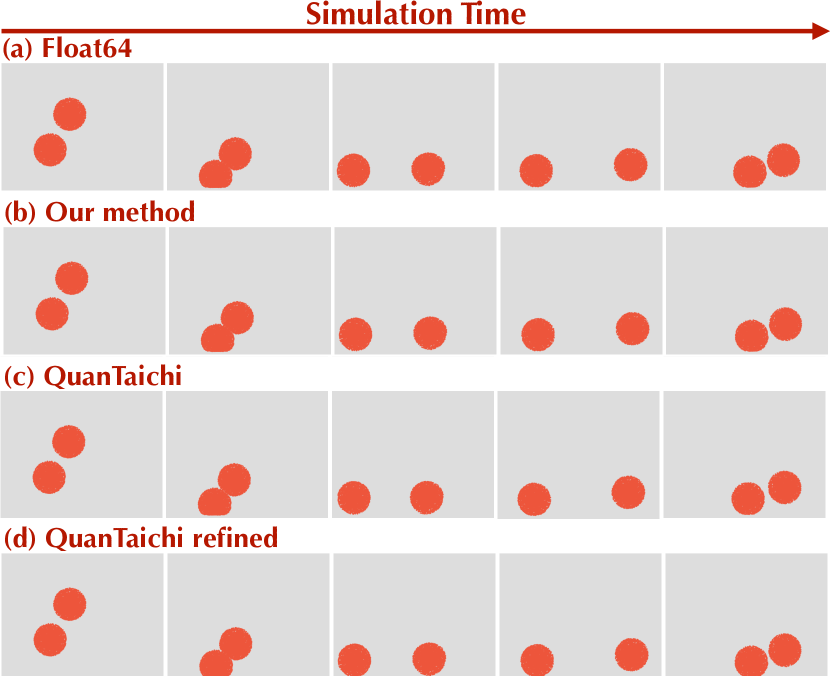
Figure 13. The comparison with human generated schemes. From top to bottom: (a) the float64 reference, (b) the result of our method, (c) the result of QuanTaichi (Hu et al., 2021), and (d) the result via a refined version of (c).As we can see from the last frame, our scheme and the refined human-generated scheme are closer to the float64 reference, while our scheme uses $12.7$% less faction bits. The vertical dashed line is added to help compare the horizontal positions of circles by different methods.

Comparison with hand-tuned schemes

We compare our method with human-generated results by reproducing the MPM ball collision experiment in QuanTaichi (Hu et al., 2021) and present the visual results in Fig. 13. We keep using the kinetic energy as the evaluation function. All the components of position, velocity and deformation gradients are quantized in the experiment. We first evaluate the error of the hand-tuned scheme $10$ times and use the mean error as the constraint. As a result, the quantization scheme derived from our optimization has $12.7$% less number of fraction bits and $94.5$% more minor error than the human-generated schemes. In the human-generated scheme, the velocity is represented by a custom float type with $6$ exponent bits and $10$ fraction bits. This data type has a larger dynamic range but has lower precision in a specific small range compared to the fixed-point data type. After we change it to a fixed-point data type and apply the ranges of our scheme for all variables, the error becomes $97.2\%$ smaller, which is very close to our scheme (see the last row of Fig. 13). The results show that our method can generate quantization schemes comparable to or even better than human experts.

Table 6. The benchmark of dithering performance on both CPU and CUDA backend. The quantization scheme can be found in the supplementary materials.

Case	Backend	Dithering	No Dithering
Store	x64	54.516s	8.888s
	CUDA	0.144s	0.059s
MatMul	x64	115.888s	16.593s
	CUDA	0.655s	0.262s
MPM 2D	x64	89.892s	59.498s
	CUDA	26.819s	26.651s
MPM 3D	CUDA	29.094s	27.284s

8.2. Performance

The techniques we presented in previous sections, such as dithering and bit pack, may have impact on the performance. We conduct several experiments to evaluate the performance impact of these techniques. Unless with further explanation, all the experiments in this section are evaluated on an NVIDIA RTX 3090 GPU with 24 GB memory and Intel Core i7-7700k with 24 GB memory.

Performance benchmark

We make a benchmark suite consisting of the following four different tasks to evaluate the running time:

Store.:

We record the time consumption of storing 512M 16-bit fixed-point numbers in to the memory ten times.

MatMul.:

Similar to the former settings, we allocate 256M $3\times 3$ matrices and multiply each with another $3\times 3$ matrix ten times. Each element of the matrix is a 16-bit fixed-point number.

MPM 2D.:

We test performance on a 2D MPM simulator with 8,000 particles, $128^{2}$ grids and 8,192 steps for five times.

MPM 3D.:

We further test the performance on a more practical application of 3D MPM simulation with 30M particles, $1024^{3}$ sparse grid and 12,800 steps.

We test the first three cases on both CPU and GPU backends and record the total time cost. However, for the 3D MPM example, we only test it on GPU backend because CPU is not suitable for this large-scale simulation in practice. We record the running time per frame for this case. The quantization schemes of the 2D/3D MPM test cases can be found in section 2 of supplementary material.

Dithering

Dithering in Sec. 5 introduces an extra random number generation step that degrades the performance. We test the influence of dithering using the benchmark and the corresponding results can be found in Table 6. Our experiments reveal that storing custom float types with dithering is a time-consuming operation, especially on a CPU backend, which slows down a memory-dense task by a factor of $8$ in the worst case. Fortunately, the performance dose not significantly decrease on CUDA and the overall simulations of the MPM 2D/3D test cases are only $1.04\times$ slower on average as shown in Table. 6. We further implement a faster random number generator to accelerate the dithering, improving the speed by $3.83\times$ on average (see Section 3.4 in the supplementary material for details).

Table 7. The benchmark of bit pack performance on CPU and CUDA backend. The quantization schemes and the data placement of the bit struct are shown in the supplementary materials.

Cases	Backend	Bit pack	Bit struct
Store	x64	7.173s	7.376s
	CUDA	0.105s	0.084s
MatMul	x64	13.608s	18.269s
	CUDA	0.159s	0.316 s
MPM 2D	x64	87.614s	112.109s
	CUDA	26.155s	26.814s
MPM 3D	CUDA	29.094s	33.232s

Bit pack

Using bit pack will lead to cases where custom data types span across two adjacent physical words, introducing one extra memory access and several bit-level operations of shifting and masking. To evaluate the performance impact, we use the performance benchmark described above with slight modifications on the quantization scheme. Specifically, we use 20-bit and 25-bit fixed-points, in the Store and MatMul cases, respectively, to create situations of custom data types across two physical words. A similar memory storage optimization strategy in QuanTaichi (Hu et al., 2021) is used to avoid atomicRMW when using bit pack. We compare the performance with bit struct in Table 7. To comprehensively evaluate the performance difference between the two data structures, we turn off dithering for the first two test cases and enable it for the two MPM cases. As can be seen from this table, the performance of bit pack is comparable to or even better than bit struct in most cases, since bit pack leads to less memory consumption on both space and bandwidth with limited disruption to spatial locality.

Bisection algorithm

We evaluate the performance of our bisection algorithm introduced in Sec. 6 on a 2D MPM solver with $5000$ particles and $128^{2}$ grids. We record the average running time of a forward simulation and a back-propagation step combined, with eight repeations and three warm-up iterations, on an NVIDIA GTX 1080Ti GPU with 11GB memory. The GPU can only contain 2000 states with a fully unfolded scheme before running out of memory, while the bisection algorithm enjoys at least $7.8\times$ larger carrying capacity in the experiment. See Fig. 6 for the comparison results.

8.3. Scalability

In this section, we describe how to obtain quantization schemes for high-resolution simulations via a scaling procedure. Specifically, we choose to first optimize for a quantization scheme using the corresponding low-resolution simulation and then apply the scheme to the high-resolution simulation. Its advantage is that we can avoid the expensive cost of high-resolution differentiable simulation in terms of both memory and computation. We demonstrate how to scale the resolution up in an example of 3D fluid simulation to verify the effectiveness of the scaling procedure, and the influence of the initial conditions on the quantization scheme is also evaluated.

We use the average height as the evaluation function in this experiment since it is approximately proportional to the fluid volume at equilibrium. For each particle, we store the position ($\mathbf{p}$), velocity ($\mathbf{v})$, the volume ratio ($J$), and the local affine velocity field ($\mathbf{C}$). These quantities add up to a total memory consumption of $48$ bytes. Starting from $0.2$M particles, we show that the unmodified quantization scheme can deliver physically-plausible results with $0.5$M, $1$M, and $5$M particles with the configurations in Table 8. While, with the help of the bisection gradient computation algorithm, we can compute gradients of a simulation with many time steps, it is still costly to directly compute the gradients for 5M or even more particles. Therefore, we use the gradients computed with 0.2M particles. The ranges are obtained via running the simulation at the highest resolution in Table 8. Finally, we set the ranges of the fixed numbers to be twice the value of the recorded maximal ranges.

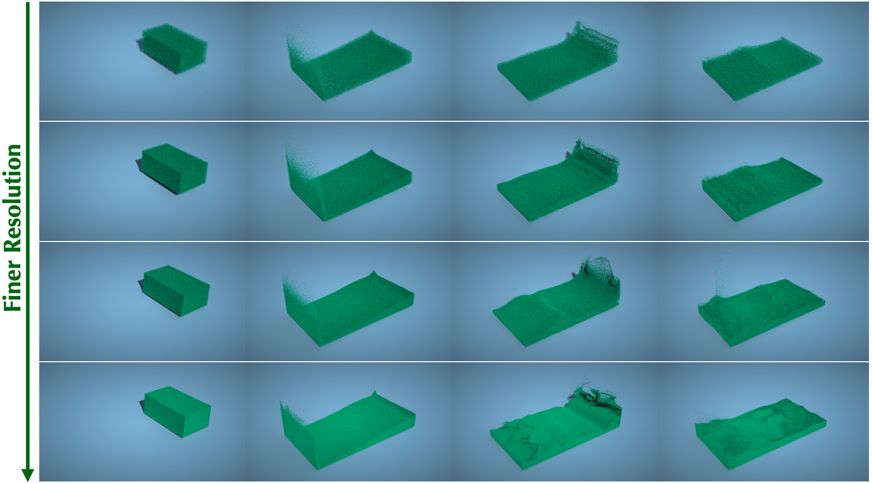
Figure 15. Visual comparisons of four simulations by gradually refining the resolution from top to bottom. All the four simulations share the same quantization scheme obtained with the first configuration in Table 8. The visual quality does not show significant degradation in the four different levels of resolution.

Table 8. Scaling configurations and the evaluations functions of the simulation. The reference evaluation function value is obtained by the float64 type. The quantized evaluation function is obtained by applying the quantization scheme derived using the first configuration. The quantization scheme can be found in the supplemental materials.

Particles	$\Delta t$	Grid	Steps	Reference Evaluation Function	Quantized Evaluation Function
200,000	$2\times 10^{-4}$	$64^{3}$	16384	$1.9910\times 10^{-2}$	$1.9908\pm 0.0004\times 10^{-2}$
500,000	$2\times 10^{-4}$	$64^{3}$	16384	$2.0130\times 10^{-2}$	$2.0543\pm 0.0019\times 10^{-2}$
1,000,000	$1\times 10^{-4}$	$128^{3}$	32768	$2.6773\times 10^{-2}$	$2.6776\pm 0.0010\times 10^{-2}$
5,000,000	$5\times 10^{-5}$	$256^{3}$	65536	$2.8241\times 10^{-2}$	$3.2300\pm 0.0015\times 10^{-2}$

Scaling up resolution.

In this experiment, we use the memory-bounded quantization to obtain a scheme with a memory compression rate of $50$%. We directly apply the scheme to the simulator with the four configurations in Table 8 with increased particle densities and keep a constant initial volume in the scaling procedure. To exploit the advantages of additional particles, we refine the background grids synchronously, which leads to a smaller time step for the sake of numerical stability. We also increase the total number of steps to match the overall duration. In the end, with all these modifications on numerous parameters, we still arrive at a large-scale physically-plausible simulation, as shown in Fig. 15 and the supplemental material.

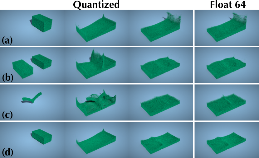
Figure 16. Simulation results under different initial conditions and parameters. The left three columns are the results of three time steps using the same quantization scheme as the scaling experiment in Fig. 15, and the last column shows the corresponding results of a float64 reference for the last time step. From top to bottom: We change the initial position and volume in rows (a) and (b); The result with an initial velocity of 2.0 is shown in row (c); The last row (d) shows the result using $4\times$ larger pressure coefficient in the fluid state equation.

Generalization to different initial conditions.

To evaluate our framework with different initial conditions, we apply the same scheme obtained in the above scaling experiment to four different initial simulation settings and show the results in Fig. 16. We use 1M particles for the four experiments and only adjust the initial position volume and velocity. We also increase the fluid pressure coefficient by a factor of $4$ to test the simulation stability (see the bottom row of Fig. 16). Our scheme can produce visual results very similar to the float64 reference. However, if we further decrease the compression rate from 50% to 30%, artifacts will appear during the simulation. For the failure case, please refer to section 2.5 in our supplementary material.

8.4. Large-scale Simulations

We show three large-scale simulation results using our method, including a 3D Eulerian smoke simulation, a 3D elastic simulation, and a fluid simulation based on MLS-MPM. The configuration details are listed in Table 9 and the rendered results are shown in Fig. 17. Their quantization schemes can be found in our supplemental materials.

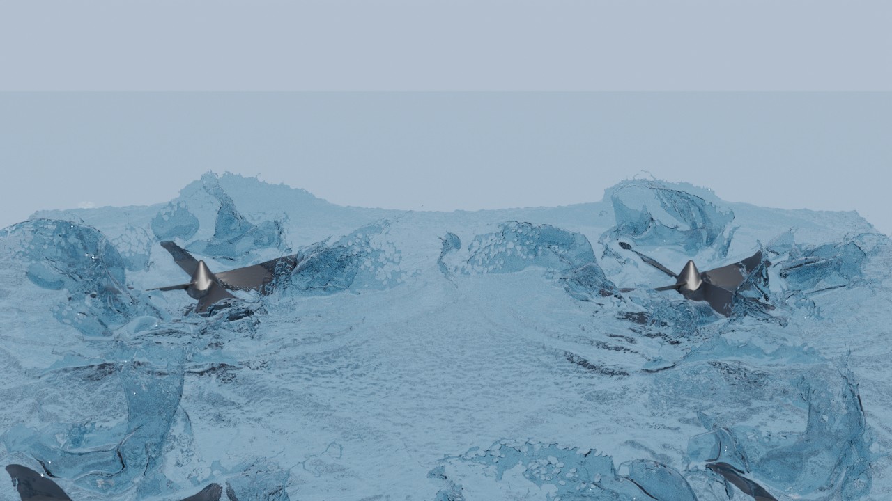
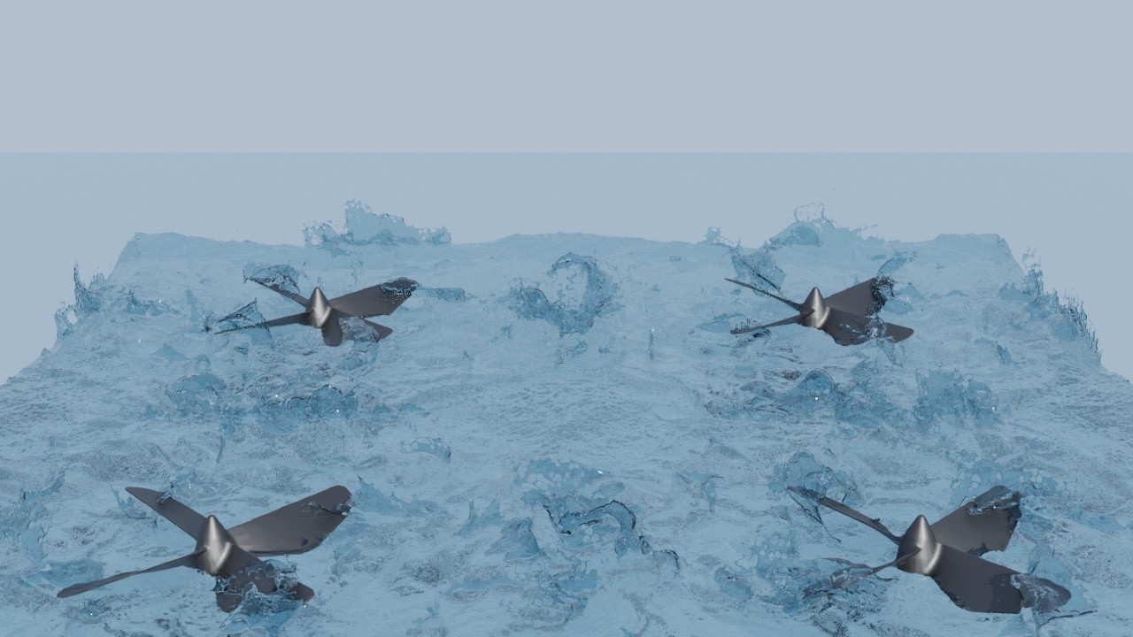
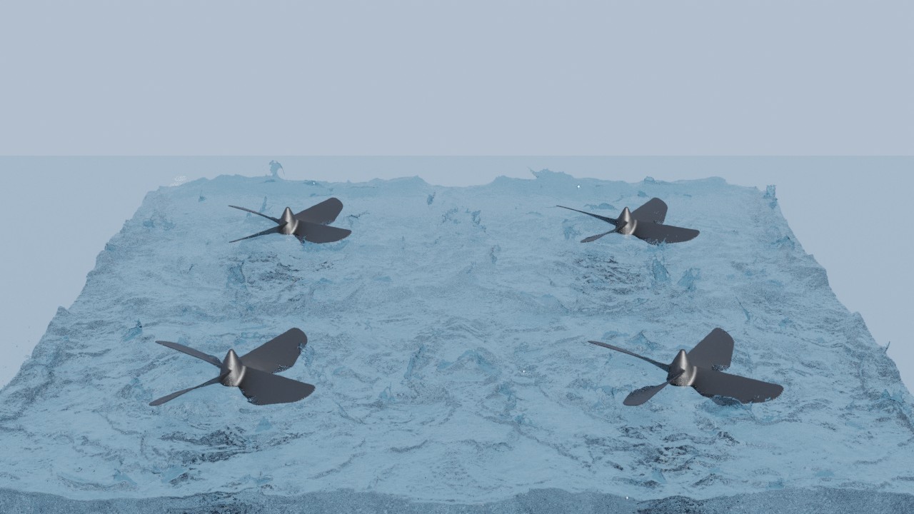
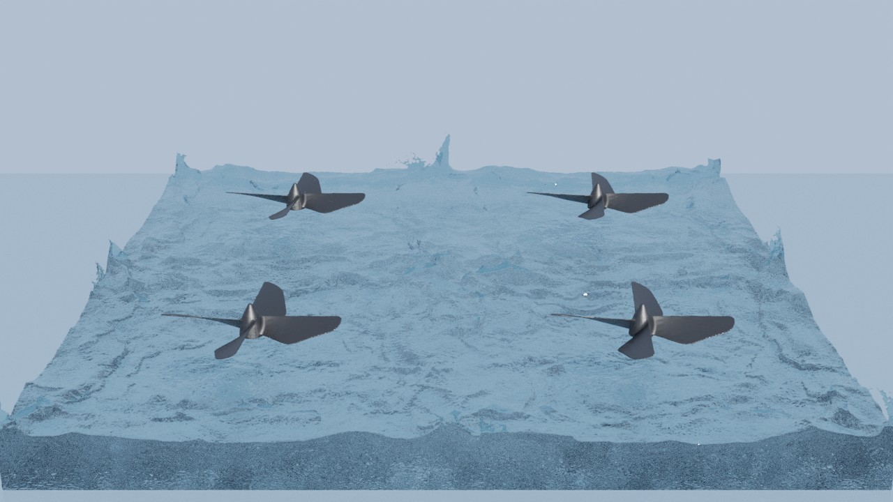
Figure 17. Snapshots of large-scale simulation results using our automatic quantized schemes.

Table 9. The configuration and results of three large-scale simulations. The elastic body and liquid simulations are based on the MLS-MPM algorithms and the smoke simulation is using an advection-reflection solver.

Demo

$\Delta t$

Particles

Grids

Frames

Steps/ Frame

Active Voxels

Memory Compression

Seconds/ Frame

Initial

Final

Initial

Final

Initial

Final

Initial

Final

Elastic body

$2\times 10^{-4}$ s

$7.5\times 10^{-5}$ s

1,000,000

295,280,208

$256^{3}$

$1024^{3}$

128

320

128

-

$2.01\times$

63.5 s

Fluid (liquid)

$4\times 10^{-4}$ s

$1\times 10^{-4}s$

1,000,000

400,000,000

$128^{3}$

$256^{3}$

128

256

128

-

$2.02\times$

139.3 s

Fluid (smoke)

0.01 s

0.01 s

-

-

$128^{3}$

$1024^{3}$

256

300

1

228,982,784

$1.93\times$

49.3 s

Eulerian smoke simulation

We develop a large-scale advection-reflection solver with the same algorithm described in Sec. 8.1. We start our workflow by computing the gradients in the float64 implementation. Then we apply the resulting scheme with a $1.93\times$ compression and eventually get a large-scale smoke simulation with over 228M voxels activated in total.

MLS-MPM simulations

We develop two large-scale MLS-MPM solvers featuring simulation of fluid and elastic body, respectively. Gradients are computed with 100M particles under $128^{3}$ and $256^{3}$ background grids, respectively. The sum of the final kinetic energy and gravitational potential energy is used as the evaluation function for both simulations. When scaling to relatively high resolution, we observe that the ranges of some attributes such as the local affine velocity $\mathbf{C}$ become much broader. To prevent the simulator from overflowing, we increase the range by $24$ times for $\mathbf{C}$ in the fluid simulation. Another way to determine the range of fixed-point numbers is evaluating the simulation at a relatively high resolution in full precision. We perform an elastic body simulation at a resolution of $125$M particles and $1024^{3}$ background grids to obtain the ranges and scale them by a factor of two. In the fluid simulation demo, we clamp the gradients during the gradients back-propagation to avoid outliers. Finally, we are able to run a fluid simulation example with $400$M particles and an elastic body simulator with $295$M particles.

9. Conclusions

We have developed a novel automatic quantization framework to determine quantization schemes, which circumvents manual trial and error and significantly improves efficiency. Users can obtain a feasible quantization scheme by simply setting a target memory compression rate or an acceptable error bound. Experimental results show that our method can generate quantization schemes that can balance the memory consumption and computation errors according to users’ preferences, which achieves up to $2.5\times$ memory compression rate without noticeable artifacts.

Limitations.

In our workflow, the quantization scheme for a high-resolution simulation is obtained via its low-resolution version, which does not take the difference between the low-resolution result and the high-resolution counterpart into account. Although the procedure of scaling up the resolution achieves reasonable results in our experiments, there is no theoretical guarantee that it can work all the time.

Future work.

We currently prefer efficiency over optimality and accept the slim possibility of failure to meet the error constraint. However, it is desirable to investigate how to speed up iterative optimization to enforce the error control more robustly. Moreover, we have only developed and tested our system on fixed-point representation, leaving the support of floating-point representation as a possible enhancement in the future.

- (1)
- Aanjaneya et al. (2017) Mridul Aanjaneya, Ming Gao, Haixiang Liu, Christopher Batty, and Eftychios Sifakis. 2017. Power diagrams and sparse paged grids for high resolution adaptive liquids. ACM Trans. Graph. 36, 4, Article 140 (2017), 12 pages.
- Bangaru et al. (2021) Sai Praveen Bangaru, Jesse Michel, Kevin Mu, Gilbert Bernstein, Tzu-Mao Li, and Jonathan Ragan-Kelley. 2021. Systematically differentiating parametric discontinuities. ACM Trans. Graph. 40, 4, Article 107 (2021), 18 pages.
- Battaglia et al. (2016) Peter Battaglia, Razvan Pascanu, Matthew Lai, Danilo Jimenez Rezende, et al. 2016. Interaction networks for learning about objects, relations and physics. In Advances in Neural Information Processing Systems. 4509–4517.
- Bouaziz et al. (2014) Sofien Bouaziz, Sebastian Martin, Tiantian Liu, Ladislav Kavan, and Mark Pauly. 2014. Projective dynamics: Fusing constraint projections for fast simulation. ACM Trans. Graph. 33, 4, Article 154 (2014), 11 pages.
- Braconnier and Langlois (2002) Thierry Braconnier and Philippe Langlois. 2002. From rounding error estimation to automatic correction with automatic differentiation. In Automatic Differentiation of Algorithms: From Simulation to Optimization. 351–357.
- Catthoor et al. (1988) Francky Catthoor, Hugo De Man, and Joos Vandewalle. 1988. Simulated-annealing-based optimization of coefficient and data word-lengths in digital filters. International Journal of Circuit Theory and Applications 16, 4 (1988), 371–390.
- Cohen (1998) E Richard Cohen. 1998. An introduction to error analysis: The study of uncertainties in physical measurements.
- Constantinides (2003) George A Constantinides. 2003. Perturbation analysis for word-length optimization. In 11th Annual IEEE Symposium on Field-Programmable Custom Computing Machines, 2003. FCCM 2003. IEEE, 81–90.
- Constantinides (2006) George A Constantinides. 2006. Word-length optimization for differentiable nonlinear systems. ACM Transactions on Design Automation of Electronic Systems (TODAES) 11, 1 (2006), 26–43.
- Constantinides et al. (2001) George A Constantinides, Peter YK Cheung, and Wayne Luk. 2001. The multiple wordlength paradigm. In The 9th Annual IEEE Symposium on Field-Programmable Custom Computing Machines (FCCM’01). IEEE, 51–60.
- de Avila Belbute-Peres et al. (2018) Filipe de Avila Belbute-Peres, Kevin Smith, Kelsey Allen, Josh Tenenbaum, and J Zico Kolter. 2018. End-to-end differentiable physics for learning and control. In Advances in Neural Information Processing Systems. 7178–7189.
- De Goes et al. (2015) Fernando De Goes, Corentin Wallez, Jin Huang, Dmitry Pavlov, and Mathieu Desbrun. 2015. Power particles: an incompressible fluid solver based on power diagrams. ACM Trans. Graph. 34, 4, Article 50 (2015), 11 pages.
- Degrave et al. (2019) Jonas Degrave, Michiel Hermans, Joni Dambre, et al. 2019. A differentiable physics engine for deep learning in robotics. Frontiers in Neurorobotics 13 (2019), 6.
- Du et al. (2021) Tao Du, Kui Wu, Pingchuan Ma, Sebastien Wah, Andrew Spielberg, Daniela Rus, and Wojciech Matusik. 2021. Diffpd: Differentiable projective dynamics. ACM Trans. Graph. 41, 2, Article 13 (2021), 21 pages.
- Ferstl et al. (2014) Florian Ferstl, Rüdiger Westermann, and Christian Dick. 2014. Large-scale liquid simulation on adaptive hexahedral grids. IEEE Transactions on Visualization and Computer Graphics 20, 10 (2014), 1405–1417.
- Gao et al. (2018) Ming Gao, Xinlei Wang, Kui Wu, Andre Pradhana, Eftychios Sifakis, Cem Yuksel, and Chenfanfu Jiang. 2018. GPU optimization of material point methods. ACM Trans. Graph. 37, 6, Article 254 (2018), 12 pages.
- Geilinger et al. (2020) Moritz Geilinger, David Hahn, Jonas Zehnder, Moritz Bächer, Bernhard Thomaszewski, and Stelian Coros. 2020. ADD: analytically differentiable dynamics for multi-body systems with frictional contact. ACM Trans. Graph. 39, 6, Article 190 (2020), 15 pages.
- Gray (1990) Robert M Gray. 1990. Quantization noise spectra. IEEE Transactions on Information Theory 36, 6 (1990), 1220–1244.
- Griewank (1992) Andreas Griewank. 1992. Achieving logarithmic growth of temporal and spatial complexity in reverse automatic differentiation. Optimization Methods and Software 1, 1 (1992), 35–54.
- Hahn and Wojtan (2015) David Hahn and Chris Wojtan. 2015. High-resolution brittle fracture simulation with boundary elements. ACM Trans. Graph. 34, 4, Article 151 (2015), 12 pages.
- Hejn and Pacut (1996) Konrad Hejn and Andrzej Pacut. 1996. Generalized model of the quantization error-a unified approach. IEEE Transactions on Instrumentation and Measurement 45, 1 (1996), 41–44.
- Hu et al. (2020) Yuanming Hu, Luke Anderson, Tzu-Mao Li, Qi Sun, Nathan Carr, Jonathan Ragan-Kelley, and Frédo Durand. 2020. DiffTaichi: Differentiable Programming for Physical Simulation. In International Conference on Learning Representations (ICLR).
- Hu et al. (2018) Yuanming Hu, Yu Fang, Ziheng Ge, Ziyin Qu, Yixin Zhu, Andre Pradhana, and Chenfanfu Jiang. 2018. A moving least squares material point method with displacement discontinuity and two-way rigid body coupling. ACM Trans. Graph. 37, 4, Article 150 (2018), 14 pages.
- Hu et al. (2019a) Yuanming Hu, Tzu-Mao Li, Luke Anderson, Jonathan Ragan-Kelley, and Frédo Durand. 2019a. Taichi: a language for high-performance computation on spatially sparse data structures. ACM Trans. Graph. 38, 6, Article 201 (2019), 16 pages.
- Hu et al. (2019b) Yuanming Hu, Jiancheng Liu, Andrew Spielberg, Joshua B Tenenbaum, William T Freeman, Jiajun Wu, Daniela Rus, and Wojciech Matusik. 2019b. Chainqueen: A real-time differentiable physical simulator for soft robotics. In International Conference on Robotics and Automation (ICRA). IEEE, 6265–6271.
- Hu et al. (2021) Yuanming Hu, Jiafeng Liu, Xuanda Yang, Mingkuan Xu, Ye Kuang, Weiwei Xu, Qiang Dai, William T. Freeman, and Frédo Durand. 2021. QuanTaichi: A Compiler for Quantized Simulations. ACM Trans. Graph. 40, 4, Article 182 (2021), 16 pages.
- Huang et al. (2021) Libo Huang, Ziyin Qu, Xun Tan, Xinxin Zhang, Dominik L. Michels, and Chenfanfu Jiang. 2021. Ships, splashes, and waves on a vast ocean. ACM Trans. Graph. 40, 6 (2021), 203:1–203:15.
- James and Pai (1999) Doug L James and Dinesh K Pai. 1999. Artdefo: accurate real time deformable objects. In Proceedings of the 26th Annual Conference on Computer Graphics and Interactive Techniques. 65–72.
- Jayant and Noll (1990) Nuggehally S. Jayant and P. Noll. 1990. Digital Coding of Waveforms: Principles and Applications to Speech and Video. Prentice Hall Professional Technical Reference.
- Keeler and Bridson (2015) Todd Keeler and Robert Bridson. 2015. Ocean Waves Animation Using Boundary Integral Equations and Explicit Mesh Tracking. In Proceedings of the ACM SIGGRAPH/Eurographics Symposium on Computer Animation. 11–19.
- Lee et al. (2006) D-U Lee, Altaf Abdul Gaffar, Ray CC Cheung, Oskar Mencer, Wayne Luk, and George A Constantinides. 2006. Accuracy-guaranteed bit-width optimization. IEEE Transactions on Computer-Aided Design of Integrated Circuits and Systems 25, 10 (2006), 1990–2000.
- Li et al. (2019) Yunzhu Li, Jiajun Wu, Russ Tedrake, Joshua B Tenenbaum, and Antonio Torralba. 2019. Learning Particle Dynamics for Manipulating Rigid Bodies, Deformable Objects, and Fluids. In International Conference on Learning Representations (ICLR).
- Liang et al. (2019) Junbang Liang, Ming C. Lin, and Vladlen Koltun. 2019. Differentiable Cloth Simulation for Inverse Problems. In Advances in Neural Information Processing Systems. 771–780.
- Liu et al. (2016) Haixiang Liu, Nathan Mitchell, Mridul Aanjaneya, and Eftychios Sifakis. 2016. A scalable schur-complement fluids solver for heterogeneous compute platforms. ACM Trans. Graph. 35, 6, Article 201 (2016), 12 pages.
- McNamara et al. (2004) Antoine McNamara, Adrien Treuille, Zoran Popović, and Jos Stam. 2004. Fluid control using the adjoint method. ACM Trans. Graph. 23, 3 (2004), 449–456.
- Moore and Yang (1996) Ramon E Moore and CT Yang. 1996. Interval analysis. Vol. 2. Prentice-Hall Englewood Cliffs, NJ.
- Museth (2013) Ken Museth. 2013. VDB: High-resolution sparse volumes with dynamic topology. ACM Trans. Graph. 32, 3, Article 27 (2013), 22 pages.
- Qiao et al. (2020) Yi-Ling Qiao, Junbang Liang, Vladlen Koltun, and Ming C. Lin. 2020. Scalable Differentiable Physics for Learning and Control. In International Conference on Machine Learning (ICML). 7847–7856.
- Sanchez-Gonzalez et al. (2020) Alvaro Sanchez-Gonzalez, Jonathan Godwin, Tobias Pfaff, Rex Ying, Jure Leskovec, and Peter Battaglia. 2020. Learning to simulate complex physics with graph networks. In International Conference on Machine Learning. 8459–8468.
- Schuchman (1964) Leonard Schuchman. 1964. Dither signals and their effect on quantization noise. IEEE Transactions on Communication Technology 12, 4 (1964), 162–165.
- Setaluri et al. (2014) Rajsekhar Setaluri, Mridul Aanjaneya, Sean Bauer, and Eftychios Sifakis. 2014. SPGrid: A sparse paged grid structure applied to adaptive smoke simulation. ACM Trans. Graph. 33, 6, Article 205 (2014), 12 pages.
- Shi and Brodersen (2004) Changchun Shi and Robert W Brodersen. 2004. A perturbation theory on statistical quantization effects in fixed-point DSP with non-stationary inputs. In 2004 IEEE International Symposium on Circuits and Systems (IEEE Cat. No. 04CH37512), Vol. 3. IEEE, III–373.
- Solenthaler and Gross (2011) Barbara Solenthaler and Markus Gross. 2011. Two-Scale Particle Simulation. ACM Trans. Graph. 30, 4, Article 81 (2011), 8 pages.
- Sung and Kum (1995) Wonyong Sung and Ki-Il Kum. 1995. Simulation-based word-length optimization method for fixed-point digital signal processing systems. IEEE Transactions on Signal Processing 43, 12 (1995), 3087–3090.
- Tampubolon et al. (2017) Andre Pradhana Tampubolon, Theodore Gast, Gergely Klár, Chuyuan Fu, Joseph Teran, Chenfanfu Jiang, and Ken Museth. 2017. Multi-species simulation of porous sand and water mixtures. ACM Trans. Graph. 36, 4, Article 105 (2017), 11 pages.
- Vakili et al. (2013) Shervin Vakili, JM Pierre Langlois, and Guy Bois. 2013. Enhanced precision analysis for accuracy-aware bit-width optimization using affine arithmetic. IEEE Transactions on Computer-Aided Design of Integrated Circuits and Systems 32, 12 (2013), 1853–1865.
- Wang et al. (2020) Xinlei Wang, Yuxing Qiu, Stuart R Slattery, Yu Fang, Minchen Li, Song-Chun Zhu, Yixin Zhu, Min Tang, Dinesh Manocha, and Chenfanfu Jiang. 2020. A massively parallel and scalable multi-GPU material point method. ACM Trans. Graph. 39, 4, Article 30 (2020), 15 pages.
- Wang et al. (2018) Zhendong Wang, Longhua Wu, Marco Fratarcangeli, Min Tang, and Huamin Wang. 2018. Parallel multigrid for nonlinear cloth simulation. Computer Graphics Forum 37, 7 (2018), 131–141.
- Wannamaker et al. (2000) Rob Wannamaker, Stanley Lipshitz, John Vanderkooy, and J. Wright. 2000. A theory of nonsubtractive dither. IEEE Transactions on Signal Processing 48 (2000), 499–516.
- Widrow (1961) B. Widrow. 1961. Statistical analysis of amplitude-quantized sampled-data systems. Transactions of the American Institute of Electrical Engineers, Part II: Applications and Industry 79, 6 (1961), 555–568.
- Wu et al. (2015) Jun Wu, Christian Dick, and Rüdiger Westermann. 2015. A system for high-resolution topology optimization. IEEE Transactions on Visualization and Computer Graphics 22, 3 (2015), 1195–1208.
- Wu et al. (2018) Kui Wu, Nghia Truong, Cem Yuksel, and Rama Hoetzlein. 2018. Fast fluid simulations with sparse volumes on the GPU. Computer Graphics Forum 37, 2 (2018), 157–167.
- Zehnder et al. (2018) Jonas Zehnder, Rahul Narain, and Bernhard Thomaszewski. 2018. An advection-reflection solver for detail-preserving fluid simulation. ACM Trans. Graph. 37, 4, Article 85 (2018), 8 pages.