Fast exchange with Gaussian basis set using robust pseudospectral method

Abstract

In this article we present an algorithm to efficiently evaluate the exchange matrix in periodic systems when Gaussian basis set with pseudopotentials are used. The usual algorithm for evaluating exchange matrix scales cubically with the system size because one has to perform $O(N^{2})$ fast Fourier transforms (FFT). Here we introduce an algorithm that retains the cubic scaling but reduces the prefactor significantly by eliminating the need to do FFTs during each exchange build. This is accomplished by representing the products of Gaussian basis function using a linear combination of an auxiliary basis the number of which scales linearly with the size of the system. We store the potential due to these auxiliary functions in memory which allows us to obtain the exchange matrix without the need to do FFT, albeit at the cost of additional memory requirement. Although the basic idea of using auxiliary functions is not new, our algorithm is cheaper due to a combination of three ingredients: (a) we use robust Pseudospectral method that allows us to use a relatively small number of auxiliary basis to obtain high accuracy (b) we use occ-RI exchange which eliminates the need to construct the full exchange matrix and (c) we use the (interpolative separable density fitting) ISDF algorithm to construct these auxiliary basis that are used in the robust pseudospectral method. The resulting algorithm is accurate and we note that the error in the final energy decreases exponentially rapidly with the number of auxiliary functions.

I Introduction

The inclusion of exact Hartree-Fock (HF) exchange within the framework of Kohn-Sham (KS) density functional theory (DFT) is critical to the success of DFT for molecular systems, and these “hybrid” functionals are used in almost all modern DFT calculations on molecules. For periodic solids, hybrid functionals can dramatically improve on standard semi-local functionals for wide variety of properties (Heyd2005, ; Kummel2008, ; Finazzi2008, ; Hai2011, ; Basera2019, ), but the large computational cost associated with computing the HF exchange is a limiting factor. The evaluation of the non-local HF exchange can be computationally demanding in any context, and it is particularly expensive for solids where calculations with hybrid density functionals may be orders of magnitude more expensive than for their purely semilocal counterparts.

Molecular calculations usually use local basis sets where the ratio of basis functions to electrons, $N/n$, is small, often on the order of 3-10. Though computation of the electron repulsion integrals is naively $O(N^{4})$, the locality of the basis implies an asymptotically linear number of significant basis function pairs and quadratic scaling of the classical Coulomb and the HF exchange (Almlof1982, ). The computation of the Coulomb energy and potential can be further reduced to $O(N)$by multipole expansion (White1994, ; Kudin1998, ), while the exchange can be computed in linear time by leveraging the sparsity of the density matrix for non-metallic systems (Challacombe1997, ; Ochsenfeld1998, ; Ko2020, ; Goedecker1999, ). This asymptotically linear region is rarely reached in practice, and recent work has focused on reducing the computational cost of practical calculations by tensor factorization. The resolution of the identity (RI) approximation (Fruchtl1998, ; Weigend2002, ), also called “density fitting,” is the most widely used such method, and efficient approaches for both Coulomb (RI-J) (Sierka2003, ; Sodt2006, ) and exchange (RI-K) (Polly2004, ; Sodt2008, ; Manzer2015, ; Manzer2015a, ) have been developed. Dunlap introduced a “robust” approximation to the 2-electron integrals for which the error in integrals is quadratic in the fitting error for the basis function products (Dunlap2000, ; Dunlap2000a, ; Hollman2017, ). The Cholesky decomposition (CD) is another method that can be used to obtain a decomposition of RI form without the need for optimized auxiliary basis sets (Beebe1977, ; Aquilante2007, ). An alternative approach, the pseudospectral (PS) method, is to provide a factorization from a real-space perspective by introducing a basis of grid points and performing one of the integrals analytically (Friesner1985, ). The chain-of-spheres exchange (COSX) algorithm (Neese2009, ) and related semi-numerical exchange algorithms(laqua18, ; Laqua20, ; Kong2017, ; kaup15, ) are a particularly general application of the PS method to exchange. The idea of factorizing the integral tensor was taken one step further in the tensor hypercontraction (THC) method of Martinez and coworkers where the 4-index 2-electron integral tensor is decomposed into a product of five 2-index tensors (Hohenstein2012, ; Parrish2012, ; Hohenstein2012a, ). The difficulty of efficiently performing the THC tensor decomposition has largely limited its use to correlated methods, but a cubic scaling factorization algorithm was first introduced by Lu and Ying (Lu2015, ) and later used to accelerate the computation of exact exchange in periodic (Hu2017, ; Dong2018, ) and molecular (Lee2020, ) calculations under the name “interpolative separable density fitting” (ISDF).

In traditional plane-wave DFT calculations, the action of the Coulomb operator on the occupied orbitals can be evaluated by solving $n$ Poisson equations. This scales quadratically in total, ($O(nN_{g}\ln N_{g})$ for $n$ electrons and $N_{g}$ grid points). In contrast, the action of the exchange operator scales cubically ($O(n^{2}N_{g}\ln N_{g})$ for $n$ electrons and $N_{g}$ grid points), a fact that has motivated the development of numerous numerical methods that seek to lessen this cost. Most notable are linear scaling methods (Goedecker1999, ; Bowler2012, ) for which the sparsity in the exchange operator relies on the system being an insulator (Wu2009, ). Stochastic density functional theory (sDFT) (Baer2013, ), including the extension to hybrid functionals (Neuhauser2016, ), can achieve linear scaling without any locality arguments, but controlling the stochastic error results in a very large prefactor. As with molecular systems, the linear regime is usually out-of-reach, and methods that do not improve the scaling, like the adaptively compressed exchange (ACE) (Lin2016, ), can greatly increase the efficiency in practice. When large supercells are necessary, a screening and/or truncating the coulomb operator in the exchange term can somewhat lessen the cost (Todorova2006, ). The auxiliary density matrix method (Guidon2010, ) (ADMM) can significantly reduce the cost by approximating the density matrix (Guidon2010, ).

In this work, we present an efficient algorithm for evaluating the exchange matrix in periodic Gaussian type orbital (GTO) calculations. We begin by providing background information that will help the reader understand the reason for high cost of exchange matrix evaluation, namely that one has to perform $O(N^{2})$ FFTs. In Section III we describe the algorithm which combines several different ideas that eliminate the need for performing FFTs during exchange build and replace them with matrix multiplications. Although the algorithm is still cubic scaling the prefactor is significantly reduced. In Section IV we describe the computational details including an efficient parallel implementation. Finally, in Section V we show that this algorithm enables computation of the exchange matrix with a cost comparable to the computation of the Coulomb matrix. This allows hybrid DFT to be used for systems where semi-local DFT is feasible.

II Background

Notation		Meaning
$n$		number of electrons
$N$		number of atom centered Gaussian basis functions
$N_{g}$		number of grid points or plane wave basis
$N_{\chi}$		number of grid points used in pseudo-spectral method
$k$		number of processors (including MPI and OMP)
$k_{t}$		number of threads per node
$\phi_{i}$ or with subscripts $i,j,k,l,\cdots$		occupied molecular orbitals
$\phi_{\mu}$ or with subscripts $\mu,\nu,\lambda,\sigma\cdots$		atom centered gaussian basis
$\chi$		pseudo-spectral fitting functions
$\mathbf{R}$		location of the grid point (or the center of the periodized Sinc basis)
$\mathbf{G}$		wave-number of the plane wave

Table 1: Notation that will be used in the rest of the paper

In this work we will solve the Hartree-Fock equations using the self-consistent field (SCF) method, where by, for a given set of molecular orbitals one constructs the Coulomb ($\hat{J}$) and the Exchange ($\hat{K}$) operators respectively. The Coulomb and exchange operators are given by the expressions

$$\hat{J}(\mathbf{r}) =\int_{\mathbb{R}^{3}}\sum_{i}\frac{|\phi_{i}(\mathbf{r}^{\prime})|^{2}}{|\mathbf{r}-\mathbf{r}^{\prime}|}d\mathbf{r}^{\prime},$$

$$\hat{K}(\mathbf{r},\mathbf{r}^{\prime}) =\sum_{i}\frac{\phi_{i}(\mathbf{r})\phi_{i}(\mathbf{r}^{\prime})}{|\mathbf{r}-\mathbf{r}^{\prime}|},$$

where $\phi_{i}(\mathbf{r})$ are the occupied molecular orbitals. From the equation one can notice that while the Coulomb operator is diagonal, the exchange operator has a rank $n$. To make progress one typically introduces a basis set and obtains the Coulomb and exchange matrices $J$ and $K$ respectively. Although many possible basis functions can be used including Slater type orbitals (Cohen2002, ; Chong2004, ), wavelets (Goedecker2009, ; yanai2015, ; Genovese2008, ; White2019, ; mrchem, ), numerical basis functions (Blum2009, ; octopus2015, ; C5CP00110B, ; Enkovaara_2010, ) etc. the two most commonly used ones are the atom-centered Gaussian basis functions (Ye2021, ; Irmler2018, ; Kuhne2020, ; Paier2009, ; Causa1988, ; Causa1988a, ; Kudin2004, ; Kudin2000, ; Sun2020, ; Lee2021, ) and the plane-wave basis (Kresse1996, ; Kresse1996a, ; Giannozzi_2017, ; GONZE2002478, ; holzwarth2005, ). Although, in this work we will use the Gaussian basis functions to represent molecular orbitals, we will also make use of the plane wave basis and their dual basis (the periodized Sinc basis) to simplify certain calculations (pulay, ; pulay2, ; Sun2017, ; Vandevondele2005, ). We first review properties of these functions.

II.1 Basis functions

We begin by introducing periodic basis functions in the unit cell defined by vectors $\mathbf{a}_{1},\mathbf{a}_{2},\mathbf{a}_{3}$, such that the volume $\Omega=\mathbf{a}_{1}\cdot(\mathbf{a}_{2}\times\mathbf{a}_{3})$. The reciprocal vectors are denoted by $\mathbf{A}_{1},\mathbf{A}_{2},\mathbf{A}_{3}$ so that $\mathbf{a}_{i}\cdot\mathbf{A}_{j}=2\pi\delta_{ij}$.

II.1.1 Plane wave basis

The plane wave basis functions $\left(\xi_{\mathbf{G}}\right)$ are parameterized by the wave-vector $\mathbf{G}$ and are given by

$$\xi_{\mathbf{G}}\left(\mathbf{r}\right)=\frac{1}{\sqrt{\Omega}}\exp\left(-i\mathbf{G}\cdot\mathbf{r}\right).$$

It is easy to check that these functions form an orthogonal basis i.e.

$$\int_{\Omega}\xi_{\mathbf{G^{\prime}}}(\mathbf{r})^{*}\xi_{\mathbf{G}}(\mathbf{r})d\mathbf{r}=\delta_{\mathbf{G^{\prime},\mathbf{G}}}$$

as long as $\mathbf{G}=n_{1}\mathbf{A}_{1}+n_{2}\mathbf{A}_{2}+n_{3}\mathbf{A}_{3}$, where $n_{i}$ are integers. If in a calculation one retains $n_{i}=-\frac{N_{i}}{2},\cdots,\frac{N_{i}+1}{2}$, where $N_{i}$ is an integer, $i=1,2,3$, then the total number of plane waves is equal to $N_{g}=N_{1}N_{2}N_{3}$.

II.1.2 Sinc basis

The dual basis consists of the periodized Sinc functions $\left(\xi_{\mathbf{R}}\right)$ (referred to as pSinc functions from now on) which are associated with grid points $\mathbf{R}$. They are obtained by the unitary transformation of the plane wave basis functions

$$\xi_{\mathbf{R}}\left(\mathbf{r}\right) =\frac{1}{\sqrt{N_{g}}}\sum_{\mathbf{G}}\exp\left(i\mathbf{G}\cdot\mathbf{R}\right)\xi_{\mathbf{G}}\left(\mathbf{r}\right)$$ (1)

$$\xi_{\mathbf{G}}\left(\mathbf{r}\right) =\frac{1}{\sqrt{N_{g}}}\sum_{\mathbf{G}}\exp\left(-i\mathbf{G}\cdot\mathbf{R}\right)\xi_{\mathbf{R}}\left(\mathbf{r}\right)$$ (2)

Again it is easy to see that $\xi_{\mathbf{R}}$ are orthogonal if $\mathbf{R}=\frac{n_{1}\mathbf{a}_{1}}{N_{1}}+\frac{n_{2}\mathbf{a}_{2}}{N_{2}}+\frac{n_{3}\mathbf{a}_{3}}{N_{3}}$ are a uniform set of grid points in the unit cell. Since the plane wave and the pSinc bases are related via a unitary transformation, they span the same space.

II.1.3 Atom-centered Gaussian basis

We also have the computational basis, the periodized atom centered Gaussian functions $\phi_{P\mu}(\mathbf{r})$ given by

$$\phi_{P\mu}\left(\mathbf{r}\right)=\sum_{\mathbf{T}}\phi_{\mu}\left(\mathbf{r}+\mathbf{T}\right),$$

where $\phi\left(\mathbf{r}\right)$ is the atom centered Gaussian and $\mathbf{T}=n_{1}\mathbf{a}_{1}+n_{2}\mathbf{a}_{2}+n_{3}\mathbf{a}_{3}$ are the lattice vectors in the real space. This function is also known as a Jacobi theta function. Note that $\phi_{P\mu}\left(\mathbf{r}\right)$ is neither orthogonal or normalized even if the functions $\phi\left(\mathbf{r}\right)$ themselves are. The periodized Gaussians can be represented as a linear combination of the plane waves ,

$$\phi_{P,\mu}\left(\mathbf{r}\right)=\sum_{\mathbf{G}}\hat{\phi}_{\mu}\left(\mathbf{G}\right)\xi_{\mathbf{G}}\left(\mathbf{r}\right)$$ (3)

where $\hat{\phi}_{\mu}\left(\mathbf{G}\right)$ is the Fourier transform of the function $\phi_{\mu}\left(\mathbf{r}\right)$,

$$\hat{\phi}_{\mu}\left(\mathbf{G}\right)=\int_{\mathbb{R}^{3}}\exp\left(i\mathbf{G}\cdot\mathbf{r}\right)\phi_{\mu}\left(\mathbf{r}\right)d\mathbf{r}$$

The Fourier transform of a Gaussian basis function is also a Gaussian, thus if

$$\phi_{\mu}(\mathbf{r})=\exp(-\mu|\mathbf{r}-\mathbf{A}_{\mu}|^{2})$$

then

$$\hat{\phi}_{\mu}(\mathbf{G})=\left(\frac{\pi}{\mu}\right)^{3/2}\frac{\exp(-|\mathbf{G}|^{2}/4/\mu)}{\sqrt{\Omega}}\exp(i\mathbf{G}\cdot\mathbf{A}_{\mu})$$ (4)

If the factor $\mu$ of the exponent of the Gaussian is small then a relatively few plane waves $N_{g}$ are needed to represent it (with a small but finite error). In this work we will use pseudo-potentials so that the Gaussian basis functions will be reasonably flat and a manageable number of plane waves is sufficient to represent them.

It is also possible to represent the periodized Gaussians as a linear combination of the pSinc basis functions,

$$\phi_{P\mu}\left(\mathbf{r}\right) =\sum_{\mathbf{R}}\tilde{\phi}_{\mu}\left(\mathbf{R}\right)\xi_{\mathbf{R}}\left(\mathbf{r}\right)$$

$$\tilde{\phi}_{\mu}\left(\mathbf{R}\right) =\frac{1}{\sqrt{N_{g}}}\sum_{\mathbf{G}}\exp\left(-i\mathbf{G}\cdot\mathbf{R}\right)\hat{\phi}_{\mu}\left(\mathbf{G}\right)$$

$$\hat{\phi}_{\mu}\left(\mathbf{G}\right) =\frac{1}{\sqrt{N_{g}}}\sum_{\mathbf{R}}\exp\left(i\mathbf{G}\cdot\mathbf{R}\right)\tilde{\phi}_{\mu}\left(\mathbf{R}\right)$$

These equations follow from (3) and (1) respectively. In what follows it will be convenient to switch from the pSinc basis to the plane-wave basis using the Fast Fourier transform (FFT), i.e. the coefficients $\tilde{\phi}_{\mu}(\mathbf{R})$ can be calculated from those of $\hat{\phi}_{\mu}(\mathbf{G})$ (and vice versa) rapidly using FFT at a cost of $O(N_{g}\ln N_{g})$.

So far we have been careful to distinguish between $\phi_{\mu}$ and $\phi_{P\mu}$, however, we will not do so for the rest of the paper where we only use the symbol $\phi_{\mu}$ and it should be understood that it refers to the periodized Gaussian function.

II.2 Integral evaluation and the diagonal approximation

In what follows we evaluate the potential due to a charge density where the charge density is given as a product of two orbitals. If we represent both orbitals $\phi_{\mu}\left(\mathbf{r}\right)$ and $\phi_{\nu}\left(\mathbf{r}\right)$ using plane wave basis, we then obtain the charge density $\rho_{\mu\nu}(\mathbf{r})$ as

$$\rho_{\mu\nu}(\mathbf{r}) =\phi_{\mu}(\mathbf{r})\phi_{\nu}(\mathbf{r})$$

$$=\frac{1}{\sqrt{\Omega}}\sum_{\mathbf{G}}^{N_{g}}\sum_{\mathbf{G}^{\prime}}^{N_{g}}\hat{\phi}_{\mu}(\mathbf{G})\hat{\phi}_{\nu}(\mathbf{G}^{\prime})\xi_{\mathbf{G}+\mathbf{G}^{\prime}}(\mathbf{r})$$

$$=\frac{1}{\sqrt{\Omega}}\sum_{\mathbf{G}}^{2N_{g}}\sum_{\mathbf{G}^{\prime}}^{N_{g}}\phi_{\mu}(\mathbf{G}-\mathbf{G}^{\prime})\hat{\phi}_{\nu}(\mathbf{G}^{\prime})\xi_{\mathbf{G}}(\mathbf{r})$$

$$\approx\frac{1}{\sqrt{\Omega}}\sum_{\mathbf{G}}^{N_{g}}\sum_{\mathbf{G}^{\prime}}^{N_{g}}\phi_{\mu}(\mathbf{G}-\mathbf{G}^{\prime})\hat{\phi}_{\nu}(\mathbf{G}^{\prime})\xi_{\mathbf{G}}(\mathbf{r}),$$

where in going from the second to the third expression we have changed the variables and in the last expression we made an approximation by truncating the summation over $\mathbf{G}$. By choosing a sufficiently large cutoff $N_{g}$, the error due to the approximation can be made negligibly small since we expect the density to be sufficiently smooth so that the contributions to $\rho_{\mu\nu}(\mathbf{G})$ coming from plane waves above the cutoff are small. With this approximation the final equation starts to look like a convolution and one can show that

$$\rho_{\mu\nu}(\mathbf{r}) \approx\frac{1}{\sqrt{\Omega}}\sum_{\mathbf{G}}^{N_{g}}\sum_{\mathbf{G}^{\prime}}^{N_{g}}\phi_{\mu}(\mathbf{G}-\mathbf{G}^{\prime})\hat{\phi}_{\nu}(\mathbf{G}^{\prime})\xi_{\mathbf{G}}(\mathbf{r})$$

$$\approx\sqrt{\frac{N_{g}}{\Omega}}\sum_{\mathbf{\mathbf{R}}}^{N_{g}}\tilde{\phi}_{\mu}(\mathbf{R})\tilde{\phi}_{\nu}(\mathbf{R})\xi_{\mathbf{R}}(\mathbf{r})$$ (5)

The last expression has been called the diagonal approximation and has been extensively used in the work of Steve White in the context of Gausslets (White2019, ; Qiu2021, ; White2017, ) and before that with Sinc functions (Jones2016, ) .

Using the diagonal approximation described above we can calculate the two-electron integrals of four Gaussian basis functions as follows

$$(\mu\nu|\lambda\sigma) =\int\int\phi_{\mu}(\mathbf{r})\phi_{\nu}(\mathbf{r})\frac{1}{|\mathbf{r}-\mathbf{r}^{\prime}|}\phi_{\lambda}(\mathbf{r}^{\prime})\phi_{\sigma}(\mathbf{r}^{\prime})d\mathbf{r}d\mathbf{r^{\prime}}$$

$$=\frac{N_{g}}{\Omega}\sum_{\mathbf{R}}\sum_{\mathbf{R}^{\prime}}\tilde{\phi}_{\mu}(\mathbf{R})\tilde{\phi}_{\nu}(\mathbf{R})\tilde{\phi}_{\lambda}(\mathbf{R}^{\prime})\tilde{\phi}_{\sigma}(\mathbf{R}^{\prime})\int\int\xi_{\mathbf{R}}(\mathbf{r})\frac{1}{|\mathbf{r}-\mathbf{r}^{\prime}|}\xi_{\mathbf{R}^{\prime}}(\mathbf{r}^{\prime})d\mathbf{r}d\mathbf{r^{\prime}}$$

$$=\frac{N_{g}}{\Omega}\sum_{\mathbf{R}}\sum_{\mathbf{R}^{\prime}}\tilde{\phi}_{\mu}(\mathbf{R})\tilde{\phi}_{\nu}(\mathbf{R})v(\mathbf{R}-\mathbf{R}^{\prime})\tilde{\phi}_{\lambda}(\mathbf{R}^{\prime})\tilde{\phi}_{\sigma}(\mathbf{R}^{\prime})$$ (6)

$$v(\mathbf{R}-\mathbf{R}^{\prime}) =\int\int\xi_{\mathbf{R}}(\mathbf{r})\frac{1}{|\mathbf{r}-\mathbf{r}^{\prime}|}\xi_{\mathbf{R}^{\prime}}(\mathbf{r}^{\prime})d\mathbf{r}d\mathbf{r^{\prime}}$$ (7)

$$=\frac{1}{N_{g}}\sum_{\mathbf{G}}\exp(-i\mathbf{G}\cdot\mathbf{R})\frac{4\pi}{G^{2}}\exp(i\mathbf{G}\cdot\mathbf{R}^{\prime})$$ (8)

In going from the first to the second expression in (6) we have used (5) and in going from the second to the third expression we have used (1) and made use of the fact that the Coulomb operator is diagonal and is equal to $\frac{4\pi}{|\mathbf{G}|^{2}}$ in plane wave basis. It is useful to note that Equation (6) takes the form of tensor hypercontraction (THC) and just like in THC one can make use of the integrals in this form to calculate exchange with a cubic scaling cost. As we will show next, the Coulomb matrix can be evaluated using a linear scaling algorithm because the matrix $v(\mathbf{R}-\mathbf{R}^{\prime})$ takes a special form shown in (7).

II.3 Coulomb matrix

In the self-consistent field calculation we construct the coulomb matrix $J_{\mu\nu}=\langle\mu|\hat{J}|\nu\rangle$ for a set of periodized Gaussian functions $\phi_{\mu}$ and $\phi_{\nu}$. Further, we represent the molecular orbitals as a linear combination of the basis functions $\phi_{i}(\mathbf{r})=\sum_{\lambda}C_{\lambda i}\phi_{P\lambda}(\mathbf{r})$, where $C_{\lambda i}$ is the matrix of molecular coefficients and we also define the density matrix $D_{\lambda\sigma}=\sum_{i}C_{\lambda i}C_{\sigma i}$. Using these, the Coulomb matrix can be written as

$$J_{\mu\nu} =\int d\mathbf{r}^{\prime}\phi_{\mu}(\mathbf{r}^{\prime})\phi_{\nu}(\mathbf{r}^{\prime})\left(\int d\mathbf{r}\frac{1}{|\mathbf{r}-\mathbf{r}^{\prime}|}\sum_{\lambda\sigma}D_{\lambda\sigma}\phi_{\lambda}(\mathbf{r})\phi_{\sigma}(\mathbf{r})\right)$$

$$=\frac{1}{\Omega}\sum_{\mathbf{R}}\left(\tilde{\phi}_{\mu}(\mathbf{R})\tilde{\phi}_{\nu}(\mathbf{R})\right)\left(\sum_{\mathbf{G}}\exp(-i\mathbf{G}\cdot\mathbf{R})\frac{4\pi}{G^{2}}\left(\sum_{\mathbf{R}^{\prime}}\exp(i\mathbf{G}\cdot\mathbf{R}^{\prime})\left(\sum_{\lambda\sigma}D_{\lambda\sigma}\tilde{\phi}_{\lambda}(\mathbf{R}^{\prime})\tilde{\phi}_{\sigma}(\mathbf{R}^{\prime})\right)\right)\right)$$

where we have made use of (6) and (7). Also the order in which the brackets are placed specify the order in which the tensor contractions are performed. Specifically, the steps involved are

1. We first evaluate the density on a grid $\rho(\mathbf{R}^{\prime})=\sum_{\lambda\sigma}D_{\lambda\sigma}\tilde{\phi}_{\lambda}(\mathbf{R}^{\prime})\tilde{\phi}_{\sigma}(\mathbf{R}^{\prime})$. This can be performed with a linear cost, since for any finite threshold, the atom centered Gaussian basis functions have a compact support, which implies that for a given $\lambda$ only an $\mathcal{O}\left(1\right)$ number of $\sigma$ have non-zero overlap.

2. Next the density in Fourier space is evaluated $\rho(\mathbf{G})=\sum_{\mathbf{R}^{\prime}}\exp(i\mathbf{G}\cdot\mathbf{R}^{\prime})\rho(\mathbf{R}^{\prime})$ which is done efficiently with $N_{g}\ln N_{g}$ cost using the FFT.

3. In the next step the potential due to this density is evaluated in real space as $V(\mathbf{R}^{\prime})=\sum_{\mathbf{G}}\exp(-i\mathbf{G}\cdot\mathbf{R})\frac{4\pi}{G^{2}}\rho(\mathbf{G})$ which can also be evaluated efficiently using FFT with an $N_{g}\ln N_{g}$ cost.

4. Finally, the Coulomb matrix is evaluated as $J_{\mu\nu}=\sum_{\mathbf{R}}\tilde{\phi}_{\mu}(\mathbf{R})\tilde{\phi}_{\nu}(\mathbf{R})V(\mathbf{R}^{\prime})$, which again is calculated with a linear scaling due to the compact support of the Gaussian basis set.

Thus, the construction of the Coulomb matrix only requires a two FFT and, the step 4 is the dominant cost of the calculation.

II.4 Exchange matrix

The exchange matrix $\langle\mu|\hat{K}|\nu\rangle$ can be constructed in a number of ways using a quartic scaling algorithm e.g. by using density fitting. However a cubic scaling algorithm is as follows,

$$K_{\mu\nu} =\sum_{i}\int\phi_{\mu}(\mathbf{r}^{\prime})\phi_{i}(\mathbf{r})\left(\int\frac{\phi_{i}(\mathbf{r}^{\prime})\phi_{\nu}(\mathbf{r}^{\prime})}{|\mathbf{r}-\mathbf{r}^{\prime}|}d\mathbf{r}^{\prime}\right)d\mathbf{r}$$

$$=\frac{1}{\Omega}\sum_{\mathbf{R}}\left(\tilde{\phi}_{\mu}(\mathbf{R})\tilde{\phi}_{i}(\mathbf{R})\right)\left(\sum_{\mathbf{G}}\exp(-i\mathbf{G}\cdot\mathbf{R})\frac{4\pi}{G^{2}}\left(\sum_{\mathbf{R}^{\prime}}\exp(i\mathbf{G}\cdot\mathbf{R}^{\prime})\tilde{\phi}_{i}(\mathbf{R}^{\prime})\tilde{\phi}_{\nu}(\mathbf{R}^{\prime})\right)\right),$$ (9)

where the order of tensor contraction is represented by the brackets. The steps involved in constructing the exchange matrix are

1. We first evaluate the product of the molecular orbital $\tilde{\phi}_{i}(\mathbf{R}^{\prime})$ and atomic orbital $\tilde{\phi}_{\nu}(\mathbf{R}^{\prime})$ on the grid to obtain $\tilde{\rho}_{i\nu}(\mathbf{R}^{\prime})=\tilde{\phi}_{i}(\mathbf{R}^{\prime})\tilde{\phi}_{\nu}(\mathbf{R}^{\prime})$, which is an $\mathcal{O}\left(1\right)$ operation for a given $i,\nu$. The value of this product density is then evaluated in the Fourier space $\tilde{\rho}_{i\nu}(\mathbf{G})$ using FFT.

2. Next the Coulomb kernel $\frac{4\pi}{G^{2}}$ multiplies $\tilde{\rho}_{i\nu}(\mathbf{G})$ and the inverse FFT is used to evaluate the potential $\tilde{V}_{i\nu}(\mathbf{R}^{\prime})$ due to $\tilde{\rho}_{i\nu}(\mathbf{R}^{\prime})$.

3. Finally, the potential is contracted with the product $\tilde{\phi}_{\mu}(\mathbf{R})\tilde{\phi}_{i}(\mathbf{R})$ to obtain the value of $K_{\mu\nu}$.

Thus one has to perform $Nn$ FFTs and inverse FFTs, one pair each for a given $i$ and $\nu$. The cost of the FFT is $N_{g}\ln N_{g}$, which makes the total cost of the exchange evaluations equal to $NnN_{g}\ln N_{g}$, where, as explained in Table 1, $N,n$ and $N_{g}$ are respectively the number of basis functions, number of electrons (or occupied orbitals) and number of grid points (or plane wave basis) respectively.

II.5 Other steps

For performing the HF calculation, one also needs the Kinetic matrix $T_{\mu\nu}$, the nuclear matrix $N_{\mu\nu}$ and the overlap matrix $S_{\mu\nu}$. These matrices are evaluated using standard techniques (sharmaBeylkina, ) and we do not discuss them further. Finally, the Fock matrix $F_{\mu\nu}=T_{\mu\nu}+N_{\mu\nu}+J_{\mu\nu}-K_{\mu\nu}$ is constructed and diagonalized to obtain the molecular coefficients $C_{\lambda i}$ using which the molecular orbitals $\phi_{i}(\mathbf{r})$ are formed. These molecular orbitals are used to construct the Fock matrix in a self-consistent field cycle. The diagonalization of the Fock matrix to obtain the molecular orbitals scales cubically, however the prefactor of this step is small so that its cost does not exceed that of Coulomb matrix construction (which scales linearly) for systems with less than 5000 basis functions (for example, see Table 4).

III Speeding up exchange evaluation

As we mentioned in the previous section, the exchange evaluation scales cubically with the size of the system. In particular, we have to perform $Nn$ FFTs. In practice, the cubic scaling in itself is not a severe limitation (at least for problems in which $\leq$5000 basis functions are utilized) since other steps such as Fock matrix diagonalization scale cubically as well. However, the high prefactor associated with performing $Nn$ FFTs results in a large overall cost. In principle, one can make evaluation of the exchange matrix to scale linearly by using the fact that $\hat{K}(\mathbf{r},\mathbf{r}^{\prime})$ decays exponentially with $|\mathbf{r}-\mathbf{r}^{\prime}|$ for systems with a band-gap or metallic systems at finite temperatures. However, even for insulating systems with reasonably large band gap the exponential decay is extremely slow and one does not reach the linear scaling regime until very large system sizes. In this work we take the point of view that by reducing the prefactor in the cubic scaling algorithm, we can obtain a method for exchange matrix formation that is only slightly more expensive than the formation of the Coulomb matrix. We briefly describe how this is accomplished before going into details in subsequent subsections.

Let us begin by observing that the number of pairs of basis function ($\phi_{\mu}\phi_{\nu}$) scale quadratically with the size of the system. However, (5) shows that by using the diagonal approximation (which can be made arbitrarily accurate) one can ensure that the products can be represented by using a linear combination of pSinc basis the number of which scales linearly with the size of the system. This fact reduces the scaling of the exchange build to cubic (from the usual quartic), however with a large prefactor. We will retain the cubic scaling but reduce the prefactor by fitting the products of gaussians using a linear combination of relatively small number of auxiliary functions. We are able to get away with using a small number of auxiliary functions because we make use of the so called robust pseudospectral method, which ensures that the error in the exchange matrix is quadratic of the error in the fitting. Below we first show how the auxiliary functions (represented by $\chi_{g}$) are obtained and then how they are used in robust pseudospectral method. Finally, we also introduce occ-RI exchange algorithm that further allows us to reduce the cost.

III.1 Interpolative separable density fitting

This algorithm was introduced by Lu and Ying (Lu2015, ) for writing down the two electron integrals in the THC format and later it was adapted for speeding up exchange matrix evaluation in hybrid DFT with plane wave basis (Hu2017, ; Dong2018, ). The basis idea is to view the product density

$$\tilde{\rho}_{\mu\nu,\mathbf{R}}=\tilde{\phi}_{\mu}(\mathbf{R})\tilde{\phi}_{\nu}(\mathbf{R})$$

as a matrix with $N^{2}$ rows corresponding to indices $\mu\nu$ and $N_{g}$ columns corresponding to the grid points. One then tries to obtain a subset of columns such that all other columns can be written as a linear combination of this subset. Specifically, we will attempt to write

$$\tilde{\rho}_{\mu\nu,\mathbf{R}}=\tilde{\phi}_{\mu}(\mathbf{R})\tilde{\phi}_{\nu}(\mathbf{R})\approx\sum_{\mathbf{R}_{g}}\tilde{\phi}_{\mu}(\mathbf{R}_{g})\tilde{\phi}_{\nu}(\mathbf{R}_{g})\chi_{g}(\mathbf{R})+O(\epsilon),$$ (10)

where $\mathbf{R}_{g}$ are a subset of all grid points that we call interpolation points, $\chi_{g}(\mathbf{R})$ is a function defined on all grid points and $\epsilon$ is the error incurred due to the approximation. The interpolation grid points $\mathbf{R}_{g}$ are obtained by performing QR decomposition with column pivoting (QRCP)(engler1997, ) on the matrix $\tilde{\rho}_{\mu\nu,\mathbf{R}}$, which allows one to write it as

$$\tilde{\rho}P=QR$$

where $P$ is a permutation matrix that ensures that the diagonal entries of the matrix $R$ are in the descending order,$R_{11}\geq R_{22}\geq R_{33}\cdots$. We then choose a user-defined $N_{\chi}$ set of interpolation points specified by the leading pivot points in $P$. These provide an optimal set of interpolation points. The cost of performing this step directly scales as $N^{2}N_{g}^{2}$ (assuming $N^{2}>N_{g}$) and is thus prohibitively expensive. It can be made to scale cubically by using a randomized algorithm and we provide more details in the Section IV.3.

Once the interpolation points are selected we can obtain the function $\chi_{g}(\mathbf{R})$ using a least square minimization

$$\min_{\chi_{\mathbf{R}_{g},\mathbf{R}}}\left|\tilde{\rho}_{\mu\nu,\mathbf{R}}-\tilde{\rho}_{\mu\nu,\mathbf{R}_{g}}\chi_{\mathbf{R}_{g},\mathbf{R}}\right|_{F},$$

where we have written $\chi_{g}(\mathbf{R})$ as a matrix $\chi_{\mathbf{R}_{g},\mathbf{R}}$, used the Einstein notation of summing over repeated indices (which we will continue to do so for the rest of this subsection) and subscript $F$ indices the Frobenius norm. The least square problem is solved by transforming it into a system of linear equations

$$\tilde{\rho}_{\mu\nu,\mathbf{R}^{\prime}_{g}}\tilde{\rho}_{\mu\nu,\mathbf{R}_{g}}\chi_{\mathbf{R}_{g},\mathbf{R}} =\tilde{\rho}_{\mu\nu,\mathbf{R}^{\prime}_{g}}\tilde{\rho}_{\mu\nu,\mathbf{R}}$$

$$X_{\mathbf{R}^{\prime}_{g},\mathbf{R}_{g}}\chi_{\mathbf{R}_{g},\mathbf{R}} =X_{\mathbf{R}^{\prime}_{g},\mathbf{R}},$$ (11)

where $X=\tilde{\rho}^{T}\tilde{\rho}$. We solve a set of $N_{g}$ linear equations of size $N_{\chi}\times N_{\chi}$ to obtain the fitting functions $\chi_{\mathbf{R}_{g},\mathbf{R}}$. A naive evaluation of $X$ will cost $N^{2}N_{g}N_{\xi}$, however, by using the product structure of $\tilde{\rho}=\tilde{\phi}_{\mu}\tilde{\phi}_{\nu}$ we reduce the cost to $NN_{g}N_{\chi}$

$$X_{\mathbf{R}^{\prime}_{g},\mathbf{R}}=\left(\tilde{\phi}_{\mu,\mathbf{R}_{g}}\tilde{\phi}_{\mu,\mathbf{R}}\right)^{2}$$

Thus, by obtaining the interpolation points using QRCP and the fitting functions by solving the least square problem we have a way of systematically improving approximation in (10). We show in Section III.2 how to use ISDF to reduce the CPU cost for exchange evaluation.

III.2 Robust fitting

Substituting equation (10) into equation (6), we obtain a set of approximate integrals

$$(\mu\nu|\lambda\sigma) \approx\frac{1}{\Omega}\sum_{\mathbf{R}_{g}}\sum_{\mathbf{R}\mathbf{R}^{\prime}}\tilde{\phi}_{\mu}(\mathbf{R}_{g})\tilde{\phi}_{\nu}(\mathbf{R}_{g})\left(\chi_{g}(\mathbf{R})\sum_{\mathbf{G}}\exp(-i\mathbf{G}\cdot\mathbf{R})\frac{4\pi}{G^{2}}\exp(i\mathbf{G}\cdot\mathbf{R}^{\prime})\right)\tilde{\phi}_{\lambda}(\mathbf{R}^{\prime})\tilde{\phi}_{\sigma}(\mathbf{R}^{\prime})+O(\epsilon)$$

$$\approx\frac{1}{\Omega}\sum_{\mathbf{R}_{g}}\sum_{\mathbf{R}^{\prime}}\tilde{\phi}_{\mu}(\mathbf{R}_{g})\tilde{\phi}_{\nu}(\mathbf{R}_{g})V(\mathbf{R}_{g},\mathbf{R}^{\prime})\tilde{\phi}_{\lambda}(\mathbf{R}^{\prime})\tilde{\phi}_{\sigma}(\mathbf{R}^{\prime})+\mathcal{O}\left(\epsilon\right)$$ (12)

where we have defined $V(\mathbf{R}_{g},\mathbf{R})$ as the potential due to the function $\chi_{g}(\mathbf{R})$. However, these integrals are not symmetric with respect to functions on the bra and ket (i.e. $(\mu\nu|\lambda\sigma)\neq(\lambda\sigma|\mu\nu)$), and consequently lead to exchange matrix that is asymmetric. The integrals can be made symmetric and more importantly the error can be made $\mathcal{O}\left(\epsilon^{2}\right)$ (which is a significant improvement over $O(\epsilon)$ error) by using the following modification

$$(\mu\nu|\lambda\sigma)\approx \frac{1}{\Omega}\sum_{\mathbf{R}_{g}}\sum_{\mathbf{R}^{\prime}}\tilde{\phi}_{\mu}(\mathbf{R}_{g})\tilde{\phi}_{\nu}(\mathbf{R}_{g})V(\mathbf{R}_{g},\mathbf{R}^{\prime})\tilde{\phi}_{\lambda}(\mathbf{R}^{\prime})\tilde{\phi}_{\sigma}(\mathbf{R}^{\prime})$$

$$+\frac{1}{\Omega}\sum_{\mathbf{R}}\sum_{\mathbf{R}_{g}}\tilde{\phi}_{\mu}(\mathbf{R})\tilde{\phi}_{\nu}(\mathbf{R})V(\mathbf{R}_{g},\mathbf{R})\tilde{\phi}_{\lambda}(\mathbf{R}_{g})\tilde{\phi}_{\sigma}(\mathbf{R}_{g})$$

$$-\frac{1}{\Omega}\sum_{\mathbf{R}^{\prime}_{g}}\sum_{\mathbf{R}_{g}}\tilde{\phi}_{\mu}(\mathbf{R}_{g})\tilde{\phi}_{\nu}(\mathbf{R}_{g})W(\mathbf{R}_{g},\mathbf{R}^{\prime}_{g})\tilde{\phi}_{\lambda}(\mathbf{R}^{\prime}_{g})\tilde{\phi}_{\sigma}(\mathbf{R}^{\prime}_{g})+\mathcal{O}\left(\epsilon^{2}\right)$$ (13)

where $W(\mathbf{R}_{g},\mathbf{R}^{\prime}_{g})$ is a symmetric matrix given by

$$W(\mathbf{R}_{g},\mathbf{R}^{\prime}_{g})=\sum_{\mathbf{R}}V(\mathbf{R}_{g},\mathbf{R})\chi_{g}(\mathbf{R})$$ (14)

To see where the qudratic error in (13) comes from, it is useful to recognize that the two electron integral is of the form $\sum_{ab}v(a)M(a,b)w(b)$. Now we can approximate $v(a)=\sum_{a_{g}}v(a_{g})\xi_{g}(a)+\epsilon\delta(a)$ and write a similar expression for $w(b)$, where $\delta(a)$ is a normalized error vector and $\epsilon$ is included to signify the magnitude of the error. Using these approxiamtions one can write

$$\sum_{ab}v(a)M(a,b)w(b)= \sum_{ab}\text{$\left(\sum_{a_{g}}v(a_{g})\xi_{g}(a)+\epsilon\delta(a)\right)$}M(a,b)\left(\sum_{b_{g}}w(b_{g})\xi_{g}(b)+\epsilon^{\prime}\delta^{\prime}(b)\right)$$

$$= \sum_{a^{\prime}b}v(a_{g})\text{$\left(\sum_{a}\xi_{g}(a)M(a,b)\right)$}w(b)+\sum_{ab^{\prime}}v(a)\text{$\left(\sum_{b}M(a,b)\xi_{g}(b)\right)$}w(b_{g})$$

$$+\sum_{a^{\prime}b^{\prime}}v(a_{g})\text{$\left(\sum_{ab}\xi_{g}(a)M(a,b)\xi_{g}(b)\right)$}w(b)+\epsilon\epsilon^{\prime}\sum_{ab}\delta(a)M(a,b)\delta^{\prime}(b)$$

The above expression is exact and in the robust pseudospectral (rPS) technique we include the first three terms and exclude the final term which is quadratic in the error $\epsilon$. The approximation made in equation (13) is known as the robust pseudospectral (rPS) and was introduced recently (Pierce2021, ). If one only includes the first line of the equation then we get the pseudospectral (PS) method and if one only uses the last line of the equation then we get the tensor hyper-contraction (THC) method. Recently, it was emphasized by Valeev et al (Pierce2021, ) that the quadratic error can be obtained by using rPS. In fact this approach has been previously used in other contexts including robust density fitting (Dunlap2000a, ; Dunlap2000, ) and even in quantum Monte Carlo for the evaluation of the reduced density matrices (Mahajan2022, ; whitlock1979properties, ; ceperley1986quantum, ; rothstein2013survey, ).

The key point is that one can evaluate the potential due to the functions $\chi_{g}(\mathbf{R})$ only at the beginning of the calculation and then during subsequent evaluations of the exchange matrix one can avoid having to do FFT. Below we show the order in which the tensor contraction can be performed to obtain the exchange matrix

$$K_{\mu\nu}=\frac{1}{\Omega}\sum_{\mathbf{R}_{g}}\tilde{\phi}_{\mu}(\mathbf{R}_{g})\left(\sum_{\mathbf{R}^{\prime}}V(\mathbf{R}_{g},\mathbf{R}^{\prime})\left(\sum_{i}\left(\sum_{\sigma}C_{\sigma i}\tilde{\phi}_{\sigma}(\mathbf{R}_{g})\right)\left(\sum_{\lambda}C_{\lambda i}\tilde{\phi}_{\lambda}(\mathbf{R}^{\prime})\right)\right)\tilde{\phi}_{\nu}(\mathbf{R}^{\prime})\right),$$ (15)

where we have only focused on the first term of equation (13) (other terms can be treated in a similar way). More explicitly, the steps involved are

1. First contraction over $\lambda$ and $\sigma$ indices is carried out to obtain molecular orbitals at all grid points ($\tilde{\phi}_{i}(\mathbf{R}^{\prime})$) and interpolation grid points ($\tilde{\phi}_{i}(\mathbf{R}_{g})$) respectively. The cost of both these calculations is $O(nN_{g})$ because of the locality of the atomic orbitals.

2. Next the contraction over $i$ is carried out to obtain the matrix $\rho(\mathbf{R}_{g},\mathbf{R}^{\prime})=\sum_{i}\tilde{\phi}_{i}(\mathbf{R}^{\prime})\tilde{\phi}_{i}(\mathbf{R}_{g})$ and the cost of this contraction is $O(nN_{g}N_{\chi})$.

3. Next we element-wise multiply $V$ and $\rho$ matrices to obtain $V_{2}(\mathbf{R}_{g},\mathbf{R}^{\prime})=V(\mathbf{R}_{g},\mathbf{R}^{\prime})\rho(\mathbf{R}_{g},\mathbf{R}^{\prime})$ which costs $O(N_{\chi}N_{g})$.

4. The matrix $V_{2}(\mathbf{R}_{g},\mathbf{R}^{\prime})$ is contracted with $\tilde{\phi}_{\mu}(\mathbf{R}_{g})$ to obtain a new matrix $M_{\mu}(\mathbf{R}^{\prime})=\sum_{\mathbf{R}_{g}}V_{2}(\mathbf{R}_{g},\mathbf{R}^{\prime})\tilde{\phi}_{\mu}(\mathbf{R}_{g})$ at a cost of $O(NN_{g}N_{\chi})$.

5. Finally, we contract over $\mathbf{R}^{\prime}$ to obtain exchange matrix $K_{\mu\nu}=\sum_{\mathbf{R}^{\prime}}M_{\mu}(\mathbf{R}^{\prime})\tilde{\phi}_{\nu}(\mathbf{R}^{\prime})$ at a cost of $O(N_{g}N^{2})$.

Given that $N_{g}>N_{\chi}>N>n$ we can see that several steps of the algorithm are cubic scaling with step 4 being the most expensive. Notice that no FFT evaluations are involved and in the result section we will show that this leads to significant speed up of the calculation.

III.3 occ-RI

If one is only interested in calculating the total energy or the energy of the occupied orbitals then it is easy to show that only the rectangular part of the Fock matrix $F_{i\mu}$ is needed, where $i$ are the labels of the occupied molecular orbitals and $\mu$ are the atomic orbitals. This was first introduced by Manzer et al (Manzer2015a, ) to reduce the cost of construction of the exchange matrix. Using $F_{i\mu}$ instead of the full $F_{\nu\mu}$matrix during the SCF cycle does not deteriorate the rate of convergence and the only drawback is that the virtual orbital energies are not evaluated correctly. However, this shortcoming can be overcome at the very end of the SCF cycle by evaluating the full matrix one time. This idea is also at the heart of the efficiency of the ACE method proposed by Lin Lin (Lin2016, ), with the difference being that the Fock matrix is not explicitly constructed but is written as a sum of outer product of $n$ vectors. This trick can readily be used with the integrals given in (13) and we obtain

$$K_{j\nu}= \sum_{\mathbf{R}^{\prime}}\left(\sum_{\mathbf{R}_{g}}\tilde{\phi}_{j}(\mathbf{R}_{g})V(\mathbf{R}_{g},\mathbf{R}^{\prime})\left(\sum_{i}\left(\sum_{\sigma}C_{\sigma i}\tilde{\phi}_{\sigma}(\mathbf{R}_{g})\right)\left(\sum_{\lambda}C_{\lambda i}\tilde{\phi}_{\lambda}(\mathbf{R}^{\prime})\right)\right)\right)\tilde{\phi}_{\nu}(\mathbf{R}^{\prime})$$

$$+\sum_{\mathbf{R}_{g}}\left(\sum_{\mathbf{R}}\tilde{\phi}_{j}(\mathbf{R})V(\mathbf{R}_{g},\mathbf{R})\left(\sum_{i}\left(\sum_{\sigma}C_{\sigma i}\tilde{\phi}_{\sigma}(\mathbf{R})\right)\left(\sum_{\lambda}C_{\lambda i}\tilde{\phi}_{\lambda}(\mathbf{R}_{g})\right)\right)\right)\tilde{\phi}_{\nu}(\mathbf{R}_{g})$$

$$-\sum_{\mathbf{R}_{g}^{\prime}}\left(\sum_{\mathbf{R}_{g}}\tilde{\phi}_{j}(\mathbf{R}_{g})W(\mathbf{R}_{g},\mathbf{R}_{g}^{\prime})\left(\sum_{i}\left(\sum_{\sigma}C_{\sigma i}\tilde{\phi}_{\sigma}(\mathbf{R}_{g})\right)\left(\sum_{\lambda}C_{\lambda i}\tilde{\phi}_{\lambda}(\mathbf{R}_{g}^{\prime})\right)\right)\right)\tilde{\phi}_{\nu}(\mathbf{R}_{g}^{\prime})$$ (16)

The cost of performing contractions in the first line is $O(nN_{\chi}N_{g})$, of second line is $O(nN_{\chi}N_{g})$ and third line is $O(nN_{\chi}^{2})$ which are all lower than the leading cost of $O(NN_{g}N_{\chi})$ of evaluating the exchange matrix without occ-RI. However, as we will see in the next section, when performing the calculation in parallel, the cost of the second step shown above is either $O(nN_{\chi}N_{g}/k)+O(nN_{\chi}N)$ or $O(NN_{g}N_{\chi}/k)$, where $k$ is the number of processors (assuming we do not want to incur additional communication overhead) and the choice between the two is not always obvious. In fact if one goes with the second choice then occ-RI provides no advantage.

IV Computational details

Having outlined the basic algorithm for fast evaluation of exchange we will outline the computational details of the program paying particular attention to the way in which it is parallelized by making use of both the message passing interface (MPI) and OpenMP (OMP) together. The summary of the memory and CPU cost of the various steps of the algorithm are displayed in Table 2 and the details are presented in the section specified in the fourth column.

Steps		Memory		CPU		Section
$\phi_{\mu}(\mathbf{R})$		$O(N_{g}/k)$		$O(NN_{g}/k)$		IV.1
$J_{\mu\nu}$		$O(N^{2})$		$O(N_{g}/k)$		IV.2
$\chi_{g}(\mathbf{R})$		$O(N_{\chi}N_{g}/k)$		$O(N_{\chi}^{3}/k_{t})$		IV.3
$V(\mathbf{R}_{g},\mathbf{R}^{\prime})$		$O(N_{\chi}N_{g}/k)$		$O((N_{\chi}N_{g}\ln N_{g})/k)$		IV.3
$W(\mathbf{R}_{g},\mathbf{R}^{\prime}_{g})$		$O(N_{\chi}^{2}/k)$		$O(N_{\chi}^{2}N_{g}/k)$		IV.3
$K_{\mu\nu}$		$O(N^{2})$		$O(nN_{\chi}N_{g}/k)+O(nN_{\chi}N)$		IV.4

Table 2: The table shows the memory and cpu cost for constructing the various tensors in the algorithm. All the symbols are defined in Table (1). For details, please see the text in the sections pointed out in the last column.

IV.1 Voronoi partitioning for each atom

We begin by partitioning the grid points $\{\mathbf{R}\}$ into disjoint set of points $\kappa_{I}$, one set for each nucleus $I$, such that all points in the set are closer to atom $I$ (or its periodic images) than any other atom (or its periodic images). The algorithm for doing Voronoi partitioning for periodic unit cells is standard (https://doi.org/10.48550/arxiv.2011.00367, ). The sets are distributed in a round robin fashion between different processors and roughly an equal number of grid points end up on each processor.

After the partitioning is performed, each processor is used to evaluate the value of periodized Gaussian basis on the grid point belonging to $\kappa_{I}$ associated with it. These values, up to a user-defined threshold $\epsilon_{1}$ (usually $10^{-8}$), are stored in memory. Thus we end up getting a different matrix $\tilde{\phi}_{\mu}^{I}(\mathbf{R})$ for each atom $I$, which specifies the values of only those functions $\mu$ that have a non-negligible value on a subset of grid points $\mathbf{R}$ in the Voronoi partition $\kappa_{I}$. The memory cost of storing this matrix is $O(1)$ because only those $\mu$ are included that have a value above $\epsilon_{1}$ for at least one grid point in $\kappa_{I}$ and due to the local nature of Gaussians, this only happens for a number of functions that are asymptotically system-size independent. The number of grid points $\mathbf{R}$ in $\kappa_{I}$ are also system size independent. Thus the total memory requirement for storing the Gaussian basis set is linear in system size and it is equally divided among the different processors, each processor stores $O(N/k)$ amount of memory. Although in principle one should be able to calculate the matrix $\tilde{\phi}_{\mu}^{I}(\mathbf{R})$ (the value of all Gaussian basis functions at all grid points) at an $O(N)$ cost by evaluating the values of the Gaussian basis functions in real space (each Gaussian has compact support up to a finise threshold). However, in our algorithm we use an $O(N^{2})$ algorithm, whereby we evaluate the value of the basis functions in the reciprocal space (recall that the Fourier transform of a Gaussian is also a Gaussian) and then we use FFT to evaluate the functions at all grid points. This procedure is more expensive but one avoids the need for lattice summations (needed for at least small unit cells) and is more convenient to implement. This calculatio is split up nearly evenly among the various processors leading to an asymptotic $O(NN_{g}/k)$ cost per processor. The cost of this step is small enough compared to the rest of the steps that even for large systems it does not become a bottleneck.

IV.2 Parallel Coulomb matrix formation

With the Gaussians stored in memory the three steps of the construction of the Coulomb matrix are evaluated in parallel on each processor. The density matrix $D_{\mu\nu}$ is replicated on each processor and first the density $\rho(\mathbf{R}^{\prime})=\sum_{\lambda\sigma}D_{\lambda\sigma}\tilde{\phi}_{\lambda}(\mathbf{R}^{\prime})\tilde{\phi}_{\sigma}(\mathbf{R}^{\prime})$ is calculated on each processor separately only for the grid points associated with it. The current algorithm is naturally linear scaling because only those basis $\lambda,\sigma$ are contracted that have a non-negligible contribution to the same Voronoi partition $\kappa_{I}$. The cumulative density is then evaluated by summing up the contributions to density coming from all processors by using the MPI command MPI_Allreduce, after which the potential is evaluated by calling FFT two times. The calls to FFT are only parallelized using OMP locally on each processor. The cost of these FFT calculations is negligible and constitute a very small fraction of the overall cost and thus not carrying it out in parallel does not cause significant overhead. Finally after the potential is obtained, the third step in which the potential is contracted with the Gaussians on the local grid to obtain the Coulomb operator $J_{\mu\nu}=\sum_{\mathbf{R}}\tilde{\phi}_{\mu}(\mathbf{R})\tilde{\phi}_{\nu}(\mathbf{R})V(\mathbf{R}^{\prime})$ is carried out on each processor and then reduced together. Thus one calculates those elements of the Coulomb operator $J_{\mu\nu}$ for which both the indices $\mu,\nu$ have non-negligible values on the Voronoi partitions associated with a given processor. However, the entire Coulomb matrix is replicated on each processor. Thus the CPU cost of the algorithm is $O(N_{g}/k)$ and the memory cost is $O(N^{2})$.

The Voronoi partitioning allows us to screen the overlap between Gaussians efficiently and results in a linear scaling algorithm that is distributed over different processors almost ideally.

IV.3 ISDF

Next we evaluate the interpolation points and the fitting functions for use in exchange build. The input to the program is a number $c$ that specifies the number of interpolation points that will be used as a factor of the number of basis functions e.g. $c=2$ means that twice as many interpolation points and fitting functions as the number of basis functions will be used. When the number of fitting functions becomes equal to $N_{g}$ then one gets the exact result. Calculating all interpolation points for the entire system scales as $O(N^{2}N_{g}^{2})$ which is prohibitive. So as a first step, a randomized algorithm (Halko2011, ; Liberty2007, ) is used to reduce the cost. In this algorithm one first constructs two random matrices $G^{1}$ and $G^{2}$ with orthogonal columns of size $N\times p$, where $p=\sqrt{N_{\chi}}+m$, where we round up $\sqrt{N_{\chi}}$ and $m$ is a small integer usually less than 5. Using these matrices we first construct the randomized density matrix

$$\tilde{\rho}_{mn,\mathbf{R}}=\left(\sum_{\mu}G_{\mu,m}^{1}\phi_{\mu}(\mathbf{R})\right)\left(\sum_{\nu}G_{\nu,m}^{2}\phi_{\nu}(\mathbf{R})\right)$$

where the size of the cumulative index $mn\sim N_{\chi}$, i.e. the number of fitting bases that will be used. The QRCP decomposition is then performed on this much smaller matrix $\tilde{\rho}_{mn,\mathbf{R}}$ instead of the full matrix $\tilde{\rho}_{\mu\nu,\mathbf{R}}$ which reduces the scaling to $O(N_{\chi}^{2}N_{g})$. The step is still fairly slow and without additional simplification can dominate the overall cost of the calculation even for small systems. Previously Dong et al. (Dong2018, ) have proposed to use a method based on centroid voronoi tessellation (CVT) with a weighted K-Mean algorithm to reduce the cost to $O(N_{\chi}N_{g})$. Here we follow a different approach. We first calculate a small subset of fitting points for each Voronoi partitioning $\kappa_{I}$ (described in section IV.1) for each atom $I$. If the number of atom centered basis functions on an atom $I$ is $N_{I}$ then we obtain a set of $\sim cN_{I}+10$ fitting points from each partition by using the same randomized QRCP as described above. Each of these calculations is extremely fast and independent of the size of the system, because both the number of grid points in $\kappa_{I}$ and the number of basis functions $N_{I}$ are small and system size independent. In the second step all these fitting points are accumulated to form a set $\{\mathbf{R}_{h}\}$ where the number of points is of similar number as $N_{\chi}$ but much smaller than $N_{g}$. Now we try to find $N_{\chi}$ interpolation points from all these $\{\mathbf{R}_{h}\}$ grid points again by using the same randomized algorithm described above, only this time we end up with a much smaller matrix

$$\tilde{\rho}_{mn,\mathbf{R}_{h}}=\left(\sum_{\mu}G_{\mu,m}^{1}\phi_{\mu}(\mathbf{R}_{h})\right)\left(\sum_{\nu}G_{\nu,m}^{2}\phi_{\nu}(\mathbf{R}_{h})\right)$$

on which one can readily perform QRCP decomposition at a cost of $O(N_{\chi}^{3})$. The QRCP is parallelized using OMP and thus the CPU cost is $O(N_{\chi}^{3}/k_{t})$, where $k_{t}$ is the number of threads per node. The construction of the interpolation points is no longer the dominant cost of the overall calculation unless one goes to very large system sizes (see Table 4). In our current implementation the QRCP is only parallelized using OMP and not using MPI+OMP. In a future publication we will use Scalapack(Scalapack, ) to further reduce the scaling from $O(N_{\chi}^{3}/k_{t})$ to $O(N_{\chi}^{3}/k)$.

Once the interpolation points have been obtained one can now calculate the fitting function $\chi_{g}(\mathbf{R})$ by solving (11). It is worth noting that it contains $N_{g}$ equations which can be solved in parallel to obtain $\chi_{g}(\mathbf{R})$ with only a subset of $\mathbf{R}$ that are associated with the processor. Thus the CPU cost of this step is $O(N_{\chi}^{3}/k_{t})+O(NN_{\chi}N_{g}/k)$. The first term arises because of the need to perform Cholesky decomposition of the matrix $X_{\mathbf{R}^{\prime}_{g},\mathbf{R}{}_{g}}$ and the term arises because of the need to solve (11). Following this one needs to obtain $W(\mathbf{R}_{g},\mathbf{R}^{\prime}_{g})$ using (14) and to do that one has to first obtain the potential $V(\mathbf{R}_{g},\mathbf{R})$ due to each function $\chi_{g}(\mathbf{R})$ (see (12)). If we view $\chi_{g}(\mathbf{R})$ as a matrix of size $N_{\chi}\times N_{g}$ then after solving the linear equations we obtain a matrix of size roughly $N_{\chi}\times\left(N_{g}/k\right)$ on each processor where we have $k$ processors, i.e. each processor contains a subset of columns of the entire matrix. To obtain the potential we first use MPI_Alltoall to obtain matrices of size $\left(N_{\chi}/k\right)\times N_{g}$ i.e. each processor now only contains a subset of rows of the entire matrix. FFT is performed in parallel on these rows to obtain the potential $V(\mathbf{R}_{g},\mathbf{R})$ where each processor again only retains a sub-matrix of size $\left(N_{\chi}/k\right)\times N_{g}$ and this results in a CPU cost of $O(N_{\chi}N_{g}\ln(N_{g})/k)$. After this a call to MPI_Alltoall is used to now distribute the matrix $V(\mathbf{R}_{g},\mathbf{R})$ with a column-wise split such that each processor ends up with a sub-matrix of size $N_{\chi}\times\left(N_{g}/k\right)$. Finally, having access to $V(\mathbf{R}_{g},\mathbf{R})$ and $\chi_{g}(\mathbf{R})$ one can evaluate the inner product defined in equation 14 to obtain $W(\mathbf{R}_{g},\mathbf{R}^{\prime}_{g})$, which can again be distributed over all processors leading to a cost of $O(N_{\chi}^{2}N_{g}/k)$. Finally, in all these calculations the matrices $\chi_{g}(\mathbf{R}),V(\mathbf{R}_{g},\mathbf{R}^{\prime}),W(\mathbf{R}_{g},\mathbf{R}^{\prime}_{g})$ are all distributed evenly among the processors and thus require a memory of $O(N_{\chi}N_{g}/k),O(N_{\chi}N_{g}/k),O(N_{\chi}^{2}/k)$ respectively.

IV.4 Parallel exchange matrix formation

As mentioned in the text below (16), when one uses the occ-RI one has two choices on how to perform contraction in the second line of the equation. One can first calculate $M_{j}(\mathbf{R}_{g})=\sum_{\mathbf{R}}\tilde{\phi}_{j}(\mathbf{R})V(\mathbf{R}_{g},\mathbf{R})$ followed by $K_{j\nu}=\sum_{\mathbf{R}_{g}}M_{j}(\mathbf{R}_{g})\tilde{\phi}_{\nu}(\mathbf{R}_{g})$ or one can reverse the order of these two contractions. In the first case, only the first step can be parallelized and the second step has to be performed on each processor and this leads to the computational cost $O(nN_{\chi}N_{g}/k)+O(nN_{\chi}N)$, while when the reversed order is used then the computational cost becomes $O(NN_{g}N_{\chi}/k)$. In practice the first algorithm tends to be faster unless the number of processors is very large, because the ratio $N_{g}/n$ can be on the order of a $10^{3}$ or more.

IV.5 Other considerations

The nuclear matrix takes the form

$$N_{\mu\nu} =\int\frac{-Z_{I}}{|\mathbf{R}_{I}-\mathbf{r}|}\rho_{\mu\nu}(\mathbf{r})d\mathbf{r}$$

$$=\frac{-Z_{I}}{\Omega}\sum_{\mathbf{G}}^{N_{g}}\frac{4\pi}{G^{2}}\exp(i\mathbf{G}\cdot\mathbf{R}_{I})\rho_{\mu\nu}(\mathbf{G})$$

where $\rho_{\mu\nu}(\mathbf{G})$ are the Fourier components of the density $\rho(\mathbf{r})=\phi_{\mu}(\mathbf{r})\phi_{\nu}(\mathbf{r})$ and here we have represented the nucleus as a delta distribution of charge $Z_{I}$ at position $\mathbf{R}_{I}$. The summation is truncated at $N_{g}$ and the largest error is incurred when both functions $\mu,\nu$ are sharp. The expression for the two electron integral for the same sharp functions is given as

$$(\mu\nu|\mu\nu)=\frac{1}{\Omega}\sum_{\mathbf{G}}^{N_{g}}\frac{4\pi}{G^{2}}\left|\rho_{\mu\nu}(\mathbf{G})\right|^{2}$$

where again the error is due to the use of a finite $N_{g}$. However, if the nuclear charge is truly assumed to be distributed as a delta function then it is clear that the error incurred in the two-electron integrals is quadratic of that of the one incurred while calculating nuclear integrals. This trend is somewhat tempered due to the fact that pseudo-potentials used in this work are not quite delta functions, but nonetheless the nuclear integrals still show the largest error. To reduce the error, we use an effectively larger $N_{g}$ while calculating the nuclear integral which has to be done only once and use a sparser grid for the rest of the calculation (including for the Coulomb and Exchange matrix formation).

In periodic systems, one often encounters the problem of linear dependencies of the Gaussian basis sets. This can be understood by looking at the equation 4, if the value of $\mu$ is smaller than $0.3/L^{2}$, where $L$ is the length of the super cell, then one can confirm that $\hat{\phi}_{\mu}(\mathbf{G})$ is effectively a constant. For small unit cells, several Gaussian functions in a standard basis set can become constants and thus are linearly dependent. However when one tries to reach the thermodynamic limit by increasing $L$ (the dimension of the super cell) then the Gaussians are no longer going to be linearly dependent and the number of linearly dependent functions do not increase linearly with the number of super cells in the system (of course the basis functions corresponding to the gamma point of the primitive unit cell are still present in the super cell which are constants). Thus in the large super cell limit we do not expect the linear dependency problem to be significantly worse than in a large relatively uniform molecule or a cluster. Nevertheless, it is true that by using Gaussian basis functions it is difficult to obtain results in the basis set limit because it is difficult to systematically improve the basis set without running into linear dependencies (which also happens for molecular systems). One way to overcome this is to use a mixed plane wave Gaussian basis set. In our algorithm it is relatively straightforward to do so such that sharp features are described by Gaussian basis function and diffuse features are described by plane wave basis functions. We will pursue this line of work in the future.

It is well known that the exchange energy has an integrable singularity which disappears in the infinite systems size limit. However, when one is using finite sized super cells then the singularity persists (note the presence of $1/\mathbf{G}^{2}$ in the denominator of equation 9) and one needs ways of regularizing it. Several approaches have been proposed (Sundararaman2013, ; Spencer08, ) to do so including using truncated coulomb (Guidon2009, ) or the minimum image convention (Tymczak2005, ; Irmler2018, ). Here we have used a very simple approach whereby we remove the $\mathbf{G}=0$ term in the exchange matrix evaluation and include a correction term $nM/2$ where $M$ is the Madelung constant of the super-cell. It is worth pointing out that one can readily use the truncated Coulomb kernel in exchange evaluation using our algorithm.

V Results

In this section we present calculations using two benchmark systems Li-H solid (Li₄H₄)_n and diamond with unit cell (C₈)_n. For both these systems we make use of the Goedecker-Teter-Hutter (GTH) pseudo-potentials (Hartwigsen98, ; Goedecker96, ) and GTH-DZVP and GTH-TZVP basis sets (Vandevondele2005, ). As pointed in the previous section the nuclear integrals are evaluated using a large $N_{g}$ cutoff (in fact part of the calculation is performed in the real space). For the calculation of the Coulomb and exchange matrix $N_{g}=35^{3}$ is used for the conventional unit cell. Numerical experiments showed that this grid is sufficient to deliver an error of less than 0.5 mHartree accuracy in Li-H system and 2 $\mu$Hartree in diamond. In this section, we first look at the relative accuracy of a single step randomized ISDF calculation versus Voronoi based one that we have proposed here. Second, we compare the accuracy of the rPS and THC approximations for obtaining the exchange energy, the accuracy of the rPS as we change the basis set and the size of the system. Finally, we present data on the cost of the calculations for Li-H of various system sizes, with the largest one being Li₂₅₆H₂₅₆ that contains 4864 basis functions.

V.1 Accuracy of approximate ISDF

		Li4H4			C8(Diamond)
$c=N_{\chi}/N$		ISDF	v-ISDF		ISDF	v-ISDF
3		$0.86$	$0.67$		$44.15$	$39.15$
4		$0.18$	$0.23$		$6.02$	$6.39$
5		$0.03$	$0.08$		$1.15$	$1.41$
6		$0.01$	$0.03$		$0.17$	$0.29$

Table 3: Error in $mE_{h}$ for Li₄H₄ and C₈(Diamond) as $N_{\chi}$ is increased with respect to results obtained with exact exchange. It is noteworthy that the errors of randomized ISDF (labeled ISDF) and voronoi-ISDF (the algorithm proposed in this work) are quite similar. The differences between the two are slightly larger than the random errors one expects to see due to the use of randomized algorithm.

In our algorithm we do not perform a single large ISDF calculation, instead we first perform a single small ISDF calculation for each atom and then do a single ISDF calculation to select the most important pivots points out of the collection of all the pivots points obtained from the individual calculations (let us call it v-ISDF for Voronoi-ISDF). Table 3 shows the error incurred in Li₄H₄ and C₈ systems when the usual randomized ISDF is used as opposed to v-ISDF. We note that the errors are quite similar pointing to the fact that the collection of pivot points that we obtain from individual ISDF calculations contain the important pivot points. One can thus devise other algorithms to select the most important points out of this small subset, including for example the K-Means algorithm presented previously(Dong2018, ). We will work on these aspects in a future publication, particularly because the single ISDF calculation needed can become expensive for large system sizes as shown in Table 4.

V.2 Accuracy of rPS vs THC

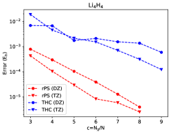
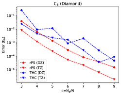
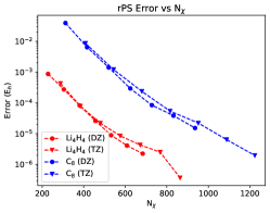
Figure 1: The left and the middle figure show the error incurred due to rPS and THC approximations in Li₄H₄ and C₈(Diamond) systems respectively. In both systems one sees that the accuracy of rPS is significantly higher than that of THC and it can be explained by the quadratic error we expect to get in the former as opposed to linear error of the latter. A noteworthy observation is that for the same value of $c$ the error is smaller with the larger basis set (TZ) rather than the smaller basis set (DZ). In fact, when one plots the error versus $N_{\chi}$ rather than $c=N_{\chi}/N$ (as is done is the right most figure) one sees that the curves for the two basis set nearly overlap, which shows that the error one makes is largely independent of the size of the basis set for a fixed number of fitting functions. Another observation is that the error is highly system dependent (see text and Figure 2)

Figure 1 shows the error as a function of $c$ when rPS and THC is used for the two systems. It is clear that the error incurred by rPS is significantly lower than THC consistent with the fact that the error in the former is expected to be square of that of the latter. Two trends stand out in the left two sub-figure. First, it appears that for the same value of $c$ the error in the larger TZ basis set is smaller than that in the smaller DZ basis set and this trend is observed for both systems. Interestingly, when one plots the error versus $N_{\chi}$rather than $c$ then the errors in the two curves nearly overlap and again this trend is observed for both systems (see right most sub-figure). Given that the cost of formation of the exchange matrix is $O(nN_{\chi}N_{g}/k)+O(nN_{\chi}N)$, we expect the cost to increase linearly with the increase in the size of the basis set $N$ (assuming $N_{\chi}$ and $N_{g}$ remain constant). The second trend one can observe is that the error decreases extremely rapidly for the Li₄H₄ as compared to the C₈(Diamond). To understand this fact, in Figure we have plotted the diagonal elements of the $R$ matrix that is obtained by performing the QR decomposition of the $\tilde{\rho}_{mn,\mathbf{R}_{h}}$ matrix. These diagonal elements reflect the importance of the various pivot points and explains why one has to include a much larger number of pivot points for C₈(Diamond) to obtain comparable accuracy. The results show that some amount of experimentation is needed to decide on the appropriate number of $c$ needed for a desired accuracy. However, the results in Figure 1 show that for both systems the results converge roughly exponentially fast with the increase in $c$.

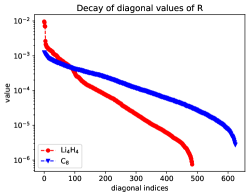
Figure 2: The figure shows diagonal elements of the R matrix obtained by performing the QR decomposition of the $\tilde{\rho}_{mn,\mathbf{R}_{h}}$ matrix. The diagonal elements decay much faster for Li₄H₄ as compared to the C₈(Diamond).

V.3 Accuracy with system size

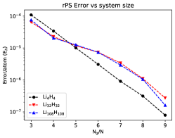
Figure 3: The intensive error (Error/atom) is approximately independent of the size of the system for the same value of $c$.

In Figure 3 we have plotted the energy/atom as a function of $c$ for three systems Li₄H₄, Li₃₂H₃₂ and Li₁₀₈H₁₀₈. The errors/atom are quite similar for the three systems and in all cases decrease exponentially with $c$. The figure indicates that one can experiment on a smaller system to estimate the value of $c$ needed for a desired accuracy and then the calculation can be scaled to larger system size.

V.4 Cost of the calculations

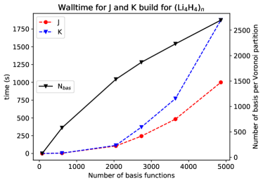
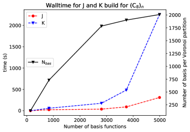
Figure 4: The red and blue curve shows the wall time needed for a single build of the Coulomb and exchange matrix on nodes containing two Intel(R) Xeon(R) CPU E5-2680 v3 @ 2.50GHz processors. The systems used to obtain this figure are (Li₄H₄)_n (lithium hydride) and (C₈)_n (diamond), where $n=1,4,8,27,36,48,64$ for the lithium hydride system and $n=1,4,8,36,48$ for diamond. For lithium hydride a $c=4$ was used and for diamond $c=6$ was used. These values of $c$are chosen to ensure that sub $mE_{h}$ errors are obtained for the $n=1$ calculation. The timings were normalized for that of 1 node, for example the largest calculation for lithium hydride contained $64$ unit cells and on the figures shows a timing of 1000 seconds for Coulomb build, however the wall time was $1000/16=62.5$ seconds on 16 nodes. The black line shows the number of basis functions with a value $>10^{-8}$ on the Voronoi partition. Note that this number is not yet a constant which leads to the super linear scaling of the Coulomb matrix construction. The relative cost of exchange is higher in diamond because a higher value of $c=6$ as opposed to $c=4$ for lithium hydride is used. Note that the cost of exchange increases linearly with $c$ while the cost of the Coulomb matrix construction is independent of it.

Figure 4 shows the cost of a single Coulomb and Exchange build for lithium hydride and diamond for various system sizes. The scaling of the Coulomb matrix appears to be non-linear mainly because the system contains highly diffuse functions that do not decay rapidly enough. For example, the black line in both the graphs shows that the number of basis functions that have a non-negligible value on the grid points of the Voronoi partition increases with the size of the system. Asymptotically this number becomes a constant but because of the presence of extremely diffuse functions this does not happen even for the largest system that contains more than a 1000 electrons. In our current implementation the grid spacing is determined by the sharpest gaussian while the number of basis functions with non-negligible value is determined by the most diffuse function. This naturally leads to a suboptimal performance in the Coulomb build. In the software packages CP2K(Kuhne2020, ) and PySCF(pyscf2018, ; pyscf2020, ) a technique known and multigrid (different than the multigrid approach used in the solution of partial differential equation) is used, whereby several grids are utilized from sparse to dense with sparse grid used to represent diffuse basis functions and the dense for sharp basis function. This allows one to reach the linear scaling regime rapidly. Another option in this context is to use (and further develop) gaussian basis set recently introduced by Ye and Berkelbach(Ye22, ) that have fewer diffuse functions which leads to fewer linear dependency problems and as a side benefit would allow one to reach the linear scaling regime more quickly without having to implement multigrid approaches. Finally, one can also replace diffuse Gaussians with plane waves which will not only allow us to more systematically increase the accuracy of the calculation but will also help reduce the overall cost by reaching the linear scaling regime sooner. We plan to pursue these lines of work in a future publication.

System		$N$		K		QRCP		$\chi_{g}(\mathbf{R})$		$W(\mathbf{R}_{g},\mathbf{R}^{\prime}_{g})$/(MPI)		Diagonalizea
Li4H4		76		1.2		1.0		0.4		1.3/(0.0)		0.0
Li32H32		608		1.0		0.3		0.3		0.7/(0.0)		0.0
Li108H108		2052		1.1		0.6		0.4		0.6/(0.3)		0.0
Li144H144		2736		1.4		0.7		0.5		0.7/(0.3)		0.0
Li192H192		3648		1.6		1.8		0.5		1.9/(1.4)		0.3
Li256H256		4864		1.9		3.9		0.6		2.9/(1.9)		0.6

Table 4: In this table we compare the cost of various steps of the algorithm relative to the cost of the Coulomb matrix construction as the size of the Lithium hydride system is increased. All calculations are $\Gamma$ point calculations and do not make use of $k$-point symmetry. For Li₄H₄ the various parameters are $n=16,N=76,N_{\chi}=304,N_{g}=42875$ and for other systems each of these parameters increase in proportion to the size of the system. Column “K” referes to the cost of exchange build, column “QRCP” refers the cost of performing of obtaining the interpolation points, column “$\chi_{g}(\mathbf{R})$” refers to the cost of obtaining the interpolation functions by solving the least square problem and column $W(\mathbf{R}_{g},\mathbf{R}^{\prime}_{g})$ refers to the cost of building the matrix $W(\mathbf{R}_{g},\mathbf{R}^{\prime}_{g})$ in (13). All Hartree-Fock calculations converged with 8 iterations and the CPU cost is relative to the cost for constructing the Coulomb matrix 8 times. In column 6, the number in brackets represents the time spent in just the MPI calls.

Table 4 shows the timings for the various steps of the calculation for a series of Li-H solids of increasing supercell size. All calculations are performed using computational nodes containing two Intel(R) Xeon(R) CPU E5-2680 v3 @ 2.50GHz processors with a total number of threads equalling 24. In all calculations a value of $c=4$ was used. From these calculations it is clear that the cost of performing QRCP to obtain the interpolation points increases quite rapidly with the systems size. This is particularly true because the QRCP is not parallelized over the number of processors and only OMP is used. We are optimistic that by using Scalapack one can reduce the cost of this step. Besides this step the cost of evaluating $W(\mathbf{R}_{g},\mathbf{R}^{\prime}_{g})$ also increases rather steeply. A significant part of the cost is incurred due to the calls to the MPI_All-to-all function which is given in the bracket of column 6. The relative cost of evaluation of the exchange matrix never increases beyond 2 compared to the Coulomb matrix even for large systems. However, for even larger systems this relative cost will keep increasing because the scaling of the two steps is not the same. Number of nodes needed increases quadratically with the size of the system because the memory cost of storing $V(\mathbf{R}_{g},\mathbf{R})$ is $N_{\chi}N_{g}$, for example 16 nodes were needed to perform the largest calculation in Table 4.

VI Conclusions

In this work we have presented an algorithm for reducing the cost of evaluation of the exchange matrix such that it is only slighly more expensive than the evaluation of the Coulomb matrix. We have done so by reducing the prefactor without changing the scaling. Currently the most expensive step of the algorithm is obtaining the interpolation points using QRCP which is cubic scaling with a fairly large over head. The QRCP cost can be decreased in two ways. First, one can parallelize the current algorithm using Scalapack to effectively make use of both the MPI and OMP, while currently we only make use of OMP. Second, we can reduce the computational cost of the algorithm as follows. In the first step of the current algorithm we obtain a set of interpolation points from each atom and in the second step we perform a large QRCP calculation to identify the most important points in this set. The second step is by far the dominant cost and this can be replaced by selecting points by using a criterion different than the QRCP method. For example, the centroid Voronoi tesselation (CVT) with K-mean algorithm (Dong2018, ) can be used to replace the last step. We expect this to be an effective approach because CVT is only used for selecting a subset of points which are already close to optimal.

In addition, the algorithm can be extended in several ways. First, we can use a mixture of plane wave and Gaussian basis function by removing diffuse Gaussians and replacing them with a set of plane wave basis. By increasing the number of plane wave basis we expect to be able to reach basis set limit when calculating energy differences (e.g. atomization energies). It remains to be seen how effective rPS algorithm remains at selecting pivot points to represent the product density of this mixed basis set. Also the number of basis functions will increase rapidly with the threshold and one will most likely have to resort to direct diagonalization. Second, our algorithm has similarities with the discontinuous Galerkin method (McClean2020, ; https://doi.org/10.48550/arxiv.2011.00367, ) and it is possible to obtain a set of Galerkin basis that are localized to a given Voronoi partition. This will have a significant advantage that the fitting functions will also be perfectly localized to an atomic domain and thus the cubic scaling of the QRCP step and the evaluation of the $W(\mathbf{R}_{g},\mathbf{R}^{\prime}_{g})$ will be reduced to linear and quadratic scaling respectively. Third, we can implement $k$-point symmetry which is expected to reduce the cost of the exchange evaluation to $O(n_{\mathbf{k}}\ln(n_{\mathbf{k}}))$ where $n_{\mathbf{k}}$ is the number of $k$-points(Jinlong2022, ). Fourth, if one wants to avoid the use of pseudo-potential then sharp gaussians are needed. To include such Gaussians one can split the solution of the Poisson’s equation between real space and reciprocal space (sharmaBeylkina, ), with real space calculations requiring the evaluation of mixed-Gaussians-plane wave integrals which we have recently developed(Beylkin2021, ). Alternatively, one has to use an irregular grid, where wavelet basis with multi resolution analysis is an attractive approach. Several wavelet basis such as interpolating wavelets, Coiflets and Gausslets allow one to use the diagonal approximation that is needed for our algorithm to work. Finally, it is possible to use the rPS integrals in correlated calculations for periodic and molecular systems.

VII Acknowledgements

AFW and SS were partly supported by the DOE grant DE-SC0022385. SS was also partly supported by NSF Career award CHE-2145209. We would also like to thank Toru Shiozaki and Daniel Moberg for helpful discussions.

References

- (1) Jochen Heyd, Juan E. Peralta, Gustavo E. Scuseria, and Richard L. Martin. Energy band gaps and lattice parameters evaluated with the Heyd-Scuseria-Ernzerhof screened hybrid functional. J. Chem. Phys., 123(17):1–8, 2005.
- (2) Stephan Kümmel and Leeor Kronik. Orbital-dependent density functionals: Theory and applications. Rev. Mod. Phys., 80(1):3–60, 2008.
- (3) Emanuele Finazzi, Cristiana Di Valentin, Gianfranco Pacchioni, and Annabella Selloni. Excess electron states in reduced bulk anatase TiO2: Comparison of standard GGA, GGA+U, and hybrid DFT calculations. J. Chem. Phys., 129(15):154113, 2008.
- (4) Xiao Hai, Jamil Tahir-Kheli, and William A. Goddard. Accurate band gaps for semiconductors from density functional theory. J. Phys. Chem. Lett., 2(3):212–217, 2011.
- (5) Pooja Basera, Shikha Saini, Ekta Arora, Arunima Singh, Manish Kumar, and Saswata Bhattacharya. Stability of non-metal dopants to tune the photo-absorption of TiO2 at realistic temperatures and oxygen partial pressures: A hybrid DFT study. Scientific Reports, 9(1):20–26, 2019.
- (6) J. Almlöf, K. Faegri, and K. Korsell. Principles for a direct SCF approach to LICAO-MO ab-initio calculations. J. Comp. Chem., 3(3):385–399, 1982.
- (7) C. A. White, B. G. Johnson, P. M. W. Gill, and M. Head-Gordon. The continuous fast multipole method. Chem. Phys. Lett., 230(1-2):8–16, 1994.
- (8) Konstantin N Kudin and Gustavo E Scuseria. A fast multipole method for periodic systems with arbitrary unit cell geometries. Technical report, 1998.
- (9) Matt Challacombe and Eric Schwegler. Linear scaling computation of the Fock matrix. The J. Chem. Phys., 106(13):5526, 1997.
- (10) Christian Ochsenfeld, Christopher a. White, and Martin Head-Gordon. Linear and sublinear scaling formation of Hartree-Fock-type exchange matrices. J. Chem. Phys., 109(5):1663, 1998.
- (11) Hsin-Yu Ko, Junteng Jia, Biswajit Santra, Xifan Wu, Roberto Car, and Robert A DiStasio Jr. Enabling Large-Scale Condensed-Phase Hybrid Density Functional Theory Based Ab Initio Molecular Dynamics. 1. Theory, Algorithm, and Performance. J Chem. Theory Comput., 16(6):3757–3785, 2020.
- (12) Stefan Goedecker. Linear scaling electronic structure methods. Rev. Mod. Phys., 71(4):1085–1123, 1999.
- (13) Herbert A. Früchtl, Rick A. Kendall, Robert J. Harrison, and Kenneth G. Dyall. An implementation of RI-SCF on parallel computers. Int. J. Quantum Chem., 64(1):63–69, 1998.
- (14) Florian Weigend. A fully direct RI-HF algorithm: Implementation, optimised auxiliary basis sets, demonstration of accuracy and efficiency. Phys. Chem. Chem. Phys., 4:4285–4291, 2002.
- (15) Marek Sierka, Annika Hogekamp, and Reinhart Ahlrichs. Fast evaluation of the Coulomb potential for electron densities using multipole accelerated resolution of identity approximation. J. Chem. Phys., 118:9136, 2003.
- (16) Alex Sodt, Joseph E. Subotnik, and Martin Head-Gordon. Linear scaling density fitting. J. Chem. Phys., 125(19):194109, 2006.
- (17) Robert Polly, Hans Joachim Werner, Frederick R. Manby, and Peter J. Knowles. Fast Hartree-Fock theory using local density fitting approximations. Mol. Phys., 102(21-22):2311–2321, 2004.
- (18) Alex Sodt and Martin Head-Gordon. Hartree-Fock exchange computed using the atomic resolution of the identity approximation. J. Chem. Phys., 128:104106, 2008.
- (19) Samuel F. Manzer, Evgeny Epifanovsky, and Martin Head-Gordon. Efficient implementation of the pair atomic resolution of the identity approximation for exact exchange for hybrid and range-separated density functionals. J. Chem. Theory Comput., 11(2):518–527, 2015.
- (20) Samuel Manzer, Paul R. Horn, Narbe Mardirossian, and Martin Head-Gordon. Fast, accurate evaluation of exact exchange: The occ-RI-K algorithm. J. Chem. Phys., 143(2):024113, 2015.
- (21) B. I. Dunlap. Robust variational fitting: Gaspar’s variational exchange can accurately be treated analytically. J. Mol. Struct.:THEOCHEM, 501-502(August):221–228, 2000.
- (22) B. I. Dunlap. Robust and variational fitting: Removing the four-center integrals from center stage in quantum chemistry. J. Mol. Struct.:THEOCHEM, 529(1-3):37–40, 2000.
- (23) David S. Hollman, Henry F. Schaefer, and Edward F. Valeev. Fast construction of the exchange operator in an atom-centred basis with concentric atomic density fitting. Mol. Phys., 115(17-18):2065–2076, 2017.
- (24) NHF Beebe and J Linderberg. Simplifications in the generation and transformation of two-electron integrals in molecular calculations. Int. J. Quantum Chem., XII:683–705, 1977.
- (25) Francesco Aquilante, Roland Lindh, and Thomas Bondo Pedersen. Unbiased auxiliary basis sets for accurate two-electron integral approximations. J. Chem. Phys., 127(11):114107, 2007.
- (26) Richard A. Friesner. Solution of self-consistent field electronic structure equations by a pseudospectral method. Chem. Phys. Lett., 116(1):39–43, 1985.
- (27) Frank Neese, Frank Wennmohs, Andreas Hansen, and Ute Becker. Efficient, approximate and parallel Hartree-Fock and hybrid DFT calculations. A ’chain-of-spheres’ algorithm for the Hartree-Fock exchange. Chem. Phys., 356(1-3):98–109, 2009.
- (28) Henryk Laqua, Travis H Thompson, Jorg Kussmann and Christian Ochsenfeld. Highly efficient, linear-scaling seminumerical exact-exchange method for graphic processing units.. J. Chem. Theory Comput., 16:1456, 2020.
- (29) Henryk Laqua, Jorg Kussmann and Christian Ochsenfeld Efficient and linear-scaling seminumerical method for local hybrid density functionals. J. Chem. Theory Comput., 14:3451, 2018.
- (30) Fenglai Liu and Jing Kong Efficient computation of exchange energy density with Gaussian basis functions. J. Chem. Theory Comput., 13:2571, 2017.
- (31) Hilke, Bahmann and Martin Kaup. Efficient self-consistent implementation of local hybrid functional. J. Chem. Theory Comput., 11:1540, 2015.
- (32) Edward G. Hohenstein, Robert M. Parrish, C. David Sherrill, and Todd J. Martínez. Communication: Tensor hypercontraction. III. Least-squares tensor hypercontraction for the determination of correlated wavefunctions. J. Chem. Phys., 137:221101, 2012.
- (33) Robert M. Parrish, Edward G. Hohenstein, Todd J. Martínez, and C. David Sherrill. Tensor hypercontraction. II. Least-squares renormalization. J. Chem. Phys., 137(22):224106, 2012.
- (34) Edward G. Hohenstein, Robert M. Parrish, and Todd J. Martínez. Tensor hypercontraction density fitting. I. Quartic scaling second- and third-order Møller-Plesset perturbation theory. J. Chem. Phys., 137(4):1085, 2012.
- (35) Jianfeng Lu and Lexing Ying. Compression of the electron repulsion integral tensor in tensor hypercontraction format with cubic scaling cost. J. Comp. Phys., 302:329–335, 2015.
- (36) Wei Hu, Lin Lin, and Chao Yang. Interpolative Separable Density Fitting Decomposition for Accelerating Hybrid Density Functional Calculations with Applications to Defects in Silicon. J. Chem. Theory Comput., 13(11):5420–5431, 2017.
- (37) Kun Dong, Wei Hu, and Lin Lin. Interpolative Separable Density Fitting through Centroidal Voronoi Tessellation with Applications to Hybrid Functional Electronic Structure Calculations. J. Chem. Theory Comput., 14(3):1311–1320, 2018.
- (38) H. Engler. The behavior of the QR-factorization algorithm with column pivoting.. Applied mathematics letters, 10(6):7-11, 1997.
- (39) Joonho Lee, Lin Lin, and Martin Head-Gordon. Systematically Improvable Tensor Hypercontraction: Interpolative Separable Density-Fitting for Molecules Applied to Exact Exchange, Second- A nd Third-Order Møller-Plesset Perturbation Theory. J. Chem. Theory Comput., 16(1):243–263, 2020.
- (40) D. R. Bowler and T. Miyazaki. O(N) methods in electronic structure calculations. Reports on Progress in Physics, 75(3):036503, 2012.
- (41) Xifan Wu, Annabella Selloni, and Roberto Car. Order- N implementation of exact exchange in extended insulating systems. Phys. Rev. B, 79:085102, 2009.
- (42) Roi Baer, Daniel Neuhauser, and Eran Rabani. Self-averaging stochastic kohn-sham density-functional theory. Phys. Rev. Lett., 111:106402, 2013.
- (43) Daniel Neuhauser, Eran Rabani, Yael Cytter, and Roi Baer. Stochastic Optimally Tuned Range-Separated Hybrid Density Functional Theory. J. Chem. Phys. A, 120(19):3071–3078, 2016.
- (44) Lin Lin. Adaptively Compressed Exchange Operator. J. Chem. Theory Comput., 12(5):2242–2249, 2016.
- (45) Teodora Todorova, Ari P. Seitsonen, Jürg Hutter, I-Feng W. Kuo, and Christopher J. Mundy. Molecular dynamics simulation of liquid water: Hybrid density functionals. The J. Chem. Phys. B, 110(8):3685–3691, 2006.
- (46) Manuel Guidon, Jürg Hutter, and Joost VandeVondele. Auxiliary Density Matrix Methods for Hartree-Fock Exchange Calculations. J. Chem. Theory Comput., 6(8):2348–2364, 2010.
- (47) Aron J. Cohen and Nicholas C. Handy. Density functional generalized gradient calculations using Slater basis sets. J. Chem. Phys., 117:1470, 2002.
- (48) Evert Jan Chong, Delano P. and Van Lenthe, Erik and Van Gisbergen, Stan and Baerends. Even-tempered slater-type orbitals revisited: From hydrogen to krypton. J. Comp. Chem., 25(8):1030–1036, 2004.
- (49) Stefan Goedecker. Wavelets and their application for the solution of partial differential equations in physics. pages —-, 2009.
- (50) Takeshi Yanai, George I Fann, Gregory Beylkin, and Robert J Harrison. Multiresolution quantum chemistry in multiwavelet bases: excited states from time-dependent Hartree-Fock and density functional theory via linear response. Phys. Chem. Chem. Phys., 17(47):31405–31416, 2015.
- (51) Luigi Genovese, Alexey Neelov, Stefan Goedecker, Thierry Deutsch, Seyed Alireza Ghasemi, Alexander Willand, Damien Caliste, Oded Zilberberg, Mark Rayson, Anders Bergman, and Reinhold Schneider. Daubechies wavelets as a basis set for density functional pseudopotential calculations. J. Chem. Phys., 129(1):14109, 2008.
- (52) Steven R. White and E. Miles Stoudenmire. Multisliced gausslet basis sets for electronic structure. Phys. Rev. B, 99(8), 2019.
- (53) Anders Brakestad, Peter Wind, Stig Rune Jensen, Luca Frediani, and Kathrin Helen Hopmann. Multiwavelets applied to metal-ligand interactions: Energies free from basis set errors. J. Chem. Phys., 154(21):214302, 2021.
- (54) Volker Blum, Ralf Gehrke, Felix Hanke, Paula Havu, Ville Havu, Xinguo Ren, Karsten Reuter, and Matthias Scheffler. Ab initio molecular simulations with numeric atom-centered orbitals. Computer Physics Communications, 180(11):2175–2196, 2009.
- (55) Xavier Andrade, David Strubbe, Umberto De Giovannini, Ask Hjorth Larsen, Micael J T Oliveira, Joseba Alberdi-Rodriguez, Alejandro Varas, Iris Theophilou, Nicole Helbig, Matthieu J Verstraete, Lorenzo Stella, Fernando Nogueira, Alán Aspuru-Guzik, Alberto Castro, Miguel A L Marques, and Angel Rubio. Real-space grids and the Octopus code as tools for the development of new simulation approaches for electronic systems. Phys. Chem. Chem. Phys., 17(47):31371–31396, 2015.
- (56) D Baye and J Dohet-Eraly. Confined helium on Lagrange meshes. Phys. Chem. Chem. Phys., 17(47):31417–31426, 2015.
- (57) J Enkovaara, C Rostgaard, J J Mortensen, J Chen, M Dułak, L Ferrighi, J Gavnholt, C Glinsvad, V Haikola, H A Hansen, H H Kristoffersen, M Kuisma, A H Larsen, L Lehtovaara, M Ljungberg, O Lopez-Acevedo, P G Moses, J Ojanen, T Olsen, V Petzold, N A Romero, J Stausholm-Møller, M Strange, G A Tritsaris, M Vanin, M Walter, B Hammer, H Häkkinen, G K H Madsen, R M Nieminen, J K Nørskov, M Puska, T T Rantala, J Schiøtz, K S Thygesen, and K W Jacobsen. Electronic structure calculations with GPAW: a real-space implementation of the projector augmented-wave method. Journal of Physics: Condensed Matter, 22(25):253202, jun 2010.
- (58) Hong Zhou Ye and Timothy C. Berkelbach. Fast periodic Gaussian density fitting by range separation. J. Chem. Phys., 154(13), 2021.
- (59) Andreas Irmler, Asbjörn M. Burow, and Fabian Pauly. Robust Periodic Fock Exchange with Atom-Centered Gaussian Basis Sets. J. Chem. Theory Comput., 14(9):4567–4580, 2018.
- (60) Thomas D. Kühne, Marcella Iannuzzi, Mauro Del Ben, Vladimir V. Rybkin, Patrick Seewald, Frederick Stein, Teodoro Laino, Rustam Z. Khaliullin, Ole Schütt, Florian Schiffmann, Dorothea Golze, Jan Wilhelm, Sergey Chulkov, Mohammad Hossein Bani-Hashemian, Valéry Weber, Urban Borštnik, Mathieu Taillefumier, Alice Shoshana Jakobovits, Alfio Lazzaro, Hans Pabst, Tiziano Müller, Robert Schade, Manuel Guidon, Samuel Andermatt, Nico Holmberg, Gregory K. Schenter, Anna Hehn, Augustin Bussy, Fabian Belleflamme, Gloria Tabacchi, Andreas Glöß, Michael Lass, Iain Bethune, Christopher J. Mundy, Christian Plessl, Matt Watkins, Joost VandeVondele, Matthias Krack, and Jürg Hutter. CP2K: An electronic structure and molecular dynamics software package -Quickstep: Efficient and accurate electronic structure calculations. J. Chem. Phys., 152:194103, 2020.
- (61) Joachim Paier, Cristian V. Diaconu, Gustavo E. Scuseria, Manuel Guidon, Joost Vandevondele, and Jürg Hutter. Accurate Hartree-Fock energy of extended systems using large Gaussian basis sets. Phys. Rev. B, 80(17):1–8, 2009.
- (62) M Causa, R Dovesi, R Orlando, Cesare Pisani, and V R Saunders. Treatment of the exchange interactions in Hartree-Fock LCAO calculations of periodic systems. The J. Chem. Phys., 92(4):909–913, feb 1988.
- (63) M. Causá, R. Dovesi, R. Orlando, C. Pisani, and V. R. Saunders. Treatment of the exchange interactions in Hartree-Fock linear combination of atomic orbital calculations of periodic systems. J. Chem. Phys., 92(4):909–913, 1988.
- (64) Konstantin N. Kudin and Gustavo E. Scuseria. Revisiting infinite lattice sums with the periodic fast multipole method. J. Chem. Phys., 121(7):2886–2890, 2004.
- (65) Konstantin N Kudin and Gustavo E Scuseria. Linear-scaling density-functional theory with Gaussian orbitals and periodic boundary conditions: Efficient evaluation of energy and forces via the fast multipole method. Phys. Rev. B, 61(24):16440–16453, jun 2000.
- (66) Qiming Sun. Exact exchange matrix of periodic hartree-fock theory for all-electron simulations. arXiv, (1):1–19, 2020.
- (67) Joonho Lee, Miguel A. Morales, and Fionn D. Malone. A phaseless auxiliary-field quantum Monte Carlo perspective on the uniform electron gas at finite temperatures: Issues, observations, and benchmark study. J. Chem. Phys., 154(6), 2021.
- (68) Georg Kresse and J Furthmuller. effective iterative schemes for ab initio total-energy calculations using a plane-wave basis set. Phys. Rev. B, 54(16):11169, 1996.
- (69) G. Kresse and J. Furthmüller. Efficiency of ab-initio total energy calculations for metals and semiconductors using a plane-wave basis set. Computational Materials Science, 6(1):15–50, 1996.
- (70) P Giannozzi, O Andreussi, T Brumme, O Bunau, M Buongiorno Nardelli, M Calandra, R Car, C Cavazzoni, D Ceresoli, M Cococcioni, N Colonna, I Carnimeo, A Dal Corso, S de Gironcoli, P Delugas, R A DiStasio, A Ferretti, A Floris, G Fratesi, G Fugallo, R Gebauer, U Gerstmann, F Giustino, T Gorni, J Jia, M Kawamura, H-Y Ko, A Kokalj, E Küçükbenli, M Lazzeri, M Marsili, N Marzari, F Mauri, N L Nguyen, H-V Nguyen, A Otero de-la Roza, L Paulatto, S Poncé, D Rocca, R Sabatini, B Santra, M Schlipf, A P Seitsonen, A Smogunov, I Timrov, T Thonhauser, P Umari, N Vast, X Wu, and S Baroni. Advanced capabilities for materials modelling with quantum ESPRESSO. Journal of Physics: Condensed Matter, 29(46):465901, oct 2017.
- (71) X. Gonze, J.-M. Beuken, R. Caracas, F. Detraux, M. Fuchs, G.-M. Rignanese, L. Sindic, M. Verstraete, G. Zerah, F. Jollet, M. Torrent, A. Roy, M. Mikami, Ph. Ghosez, J.-Y. Raty, and D.C. Allan. First-principles computation of material properties: the abinit software project. Computational Materials Science, 25(3):478–492, 2002.
- (72) N. A. W. Holzwarth, G. E. Matthews, R. B. Dunning, A. R. Tackett, and Y. Zeng. Comparison of the projector augmented-wave, pseudopotential, and linearized augmented-plane-wave formalisms for density-functional calculations of solids. Phys. Rev. B, 55:2005–2017, Jan 1997.
- (73) Laszlo Fusti-Molnar and Peter Pulay. The Fourier transform coulomb method: Efficient and accurate calculation of the coulomb operator in a gaussian basis. J. Chem. Phys., 117:7827–7835, 2002.
- (74) Laszlo Fusti-Molnar and Peter Pulay. Accurate molecular integrals and energies using combined plane wave and gaussian basis sets in molecular electronic structure theory. J. Chem. Phys., 116:7795–7805, 2002.
- (75) Qiming Sun, Timothy C. Berkelbach, James D. McClain, and Garnet Kin Lic Chan. Gaussian and plane-wave mixed density fitting for periodic systems. J. Chem. Phys., 147(16), 2017.
- (76) Joost Vandevondele, Matthias Krack, Fawzi Mohamed, Michele Parrinello, Thomas Chassaing, and Jürg Hutter. Quickstep: Fast and accurate density functional calculations using a mixed Gaussian and plane waves approach. Computer Physics Communications, 167(2):103–128, 2005.
- (77) Yiheng Qiu and Steven R. White. Hybrid gausslet/Gaussian basis sets. 2021.
- (78) Steven R. White. Hybrid grid/basis set discretizations of the Schrödinger equation. J. Chem. Phys., 147(24), 2017.
- (79) Jeremiah R. Jones, François Henry Rouet, Keith V. Lawler, Eugene Vecharynski, Khaled Z. Ibrahim, Samuel Williams, Brant Abeln, Chao Yang, William McCurdy, Daniel J. Haxton, Xiaoye S. Li, and Thomas N. Rescigno. An efficient basis set representation for calculating electrons in molecules. Mol. Phys., 114(13):2014–2028, 2016.
- (80) Sandeep Sharma and Gregory Beylkin. Efficient evaluation of two-center gaussian integrals in periodic systems. J. Chem. Theory Comput., 17(7):3916–3922, 2021. PMID: 34061523.
- (81) Karl Pierce, Varun Rishi, and Edward F. Valeev. Robust Approximation of Tensor Networks: Application to Grid-Free Tensor Factorization of the Coulomb Interaction. J. Chem. Theory Comput., 17(4):2217–2230, 2021.
- (82) Ankit Mahajan, Joonho Lee, and Sandeep Sharma. Selected configuration interaction wave functions in phaseless auxiliary field quantum monte carlo. J. Chem. Phys., 156(17):174111, 2022.
- (83) P_A Whitlock, DM Ceperley, GV Chester, and MH Kalos. Properties of liquid and solid he 4. Phys. Rev. B, 19(11):5598, 1979.
- (84) David M Ceperley and MH Kalos. Quantum many-body problems. In Monte Carlo methods in statistical physics, pages 145–194. Springer, 1986.
- (85) Stuart M Rothstein. A survey on pure sampling in quantum monte carlo methods. Canadian Journal of Chemistry, 91(7):505–510, 2013.
- (86) Fabian M. Faulstich, Xiaojie Wu, and Lin Lin. Discontinuous galerkin method with voronoi partitioning for quantum simulation of chemistry, 2020.
- (87) N Halko, P G Martinsson, and J A Tropp. Finding Structure with Randomness: Probabilistic Algorithms for Constructing Approximate Matrix Decompositions. SIAM Review, 53(2):217–288, 2011.
- (88) Edo Liberty, Franco Woolfe, Per-Gunnar Martinsson, Vladimir Rokhlin, and Mark Tygert. Randomized algorithms for the low-rank approximation of matrices. Proceedings of the National Academy of Sciences, 104(51):20167–20172, 2007.
- (89) L. S. Blackford, J. Choi, A. Cleary, E. D’Azevedo, J. Demmel, I. Dhillon, J. Dongarra, S. Hammarling, G. Henry, A. Petitet, K. Stanley, D. Walker, and R. C. Whaley. ScaLAPACK Users’ Guide. Society for Industrial and Applied Mathematics: Philadelphia, PA, 1997.
- (90) Ravishankar Sundararaman and T. A. Arias. Regularization of the Coulomb singularity in exact exchange by Wigner-Seitz truncated interactions: Towards chemical accuracy in nontrivial systems. Phys. Rev. B, 87(16), 2013.
- (91) James Spencer and Ali Alavi. Efficient calculation of the exact exchange energy in periodic systems using a truncated Coulomb potential. Phys. Rev. B, 77(19):193110, may 2008.
- (92) Manuel Guidon, Jürg Hutter, and Joost VandeVondele. Robust periodic Hartree-Fock exchange for large-scale simulations using Gaussian basis sets. J. Chem. Theory Comput., 5(11):3010–3021, 2009.
- (93) C J Tymczak, Valéry T Weber, Eric Schwegler, and Matt Challacombe. Linear scaling computation of the Fock matrix. VIII. Periodic boundaries for exact exchange at the Gamma point. J. Chem. Phys., 122(12):124105, mar 2005.
- (94) C. Hartwigsen, S. Goedecker, and J. Hutter. Relativistic separable dual-space gaussian pseudopotentials from h to rn. Phys. Rev. B, 58:3641–3662, Aug 1998.
- (95) S. Goedecker, M. Teter, and J. Hutter. Separable dual-space gaussian pseudopotentials. Phys. Rev. B, 54:1703–1710, Jul 1996.
- (96) Qiming Sun, Xing Zhang, Samragni Banerjee, Peng Bao, Marc Barbry, Nick S. Blunt, Nikolay A. Bogdanov, and George H. Booth, Jia Chen, Zhi-Hao Cui, Janus J. Eriksen, Yang Gao, Sheng Guo, Jan Hermann, Matthew R. Hermes, Kevin Koh, and Peter Koval, Susi Lehtola, Zhendong Li, Junzi Liu, Narbe Mardirossian, James D. McClain, Mario Motta, Bastien Mussard, Hung Q. Pham, Artem Pulkin, Wirawan Purwanto, Paul J. Robinson, Enrico Ronca, Elvira R. Sayfutyarova, Maximilian Scheurer, Henry F. Schurkus, James E. T. Smith, Chong Sun, Shi-Ning Sun, Shiv Upadhyay, Lucas K. Wagner, Xiao Wang, Alec White, James Daniel Whitfield, Mark J. Williamson, Sebastian Wouters, Jun Yang, Jason M. Yu, Tianyu Zhu, Timothy C. Berkelbach, Sandeep Sharma, Alexander Yu. Sokolov and Garnet Kin-Lic Chan. Recent developments in the PySCF program package J. Chem. Phys., 153:024109, 2020.
- (97) Qiming Sun, Timothy C. Berkelbach, Nick S. Blunt, George H. Booth, Sheng Guo, Zhendong Li, Junzi Liu, James D. McClain, Elvira R. Sayfutyarova, Sandeep Sharma, Sebastian Wouters, and Garnet Kin-Lic Chan. PySCF: the Python-based simulations of chemistry framework WIREs Computational Molecular Science, 8:e1304, 2018.
- (98) Hong-Zhou Ye, and Timothy C. Berkelbach, Correlation-Consistent Gaussian Basis Sets for Solids Made Simple J. Chem. Theory Comput., 18:1595, 2022.
- (99) Jarrod R. McClean, Fabian M. Faulstich, Qinyi Zhu, Bryan O’Gorman, Yiheng Qiu, Steven R. White, Ryan Babbush, and Lin Lin. Discontinuous Galerkin discretization for quantum simulation of chemistry. New Journal of Physics, 22(9):1–21, 2020.
- (100) Gregory Beylkin and Sandeep Sharma. A fast algorithm for computing the boys function. J. Chem. Phys., 155(17):174117, 2021.
- (101) Kai Wu, Xinming Qin, Wei Hu and Jinlong Yang. Low-Rank Approximation Accelerated Plane-Wave Hybrid Functional Calculations with k-point Sampling.. J. Chem. Theory Comput., 18(1):206, 2022.