A multivariate semi-parametric portfolio risk optimization and forecasting framework

Abstract

We develop a novel multivariate semi-parametric modelling approach to portfolio Value-at-Risk (VaR) and Expected Shortfall (ES) forecasting. Differently from existing univariate semi-parametric approaches, the proposed framework involves explicit modelling of the dependence structure among portfolio asset returns through a dynamic conditional correlation (DCC) parameterization. Model parameters are estimated through a two-step procedure based on the minimization of strictly consistent scoring functions derived from the Asymmetric Laplace (AL) distribution. The proposed model is consequently denominated as DCC-AL. The performance of the DCC-AL in risk forecasting and portfolio optimization is assessed by means of a forecasting study on the components of the Dow Jones index for an out-of-sample period from December 2016 to September 2021. The empirical results support the proposed model class, comparing to a variety of existing approaches, in terms of risk forecasting and portfolio optimization.

Keywords: semi-parametric; Value-at-Risk; Expected Shortfall; multivariate; portfolio optimization.

1 Introduction

Value-at-Risk (VaR) and Expected Shortfall (ES) play a central role in the risk management systems of banks and other financial institutions. For more than two decades, VaR has been the official risk measure adopted worldwide by financial intermediaries operating in the global financial system. Nevertheless, VaR has some important theoretical limits. First, VaR cannot measure the expected loss for extreme (violating) returns. In addition, it can be shown that VaR is not always a coherent risk measure, due to failure to match the subadditivity property. For these reasons, the Basle Committee on Banking Supervision proposed in May 2012 to replace VaR with the ES (Artzner 1997; Artzner et al. 1999). ES is defined as the expectation of the return conditional on it having exceeded the VaR. Differently from VaR, ES is a coherent measure and “measures the riskiness of a position by considering both the size and the likelihood of losses above a certain confidence level” (Basel Committee on Banking Supervision, 2013). Thus, in recent years ES has been increasingly employed for tail risk measurement.

Comparing to VaR, there is much less existing work on modeling ES, which is partly due to the non-elicitability of ES alone. However, the recent work in Fissler and Ziegel (2016) has shown that the pair (VaR,ES) is jointly elicitable. They develop a family of joint loss, or scoring, functions that are strictly consistent for the true VaR and ES, i.e., they are uniquely minimized by the true VaR and ES series. This result has important implications for the estimation of conditional VaR and ES as well as for ranking risk forecasts from alternative competing models. Taylor (2019) proposes a joint VaR and ES modelling approach (named as ES-CAViaR in this paper) based on the minimization of the negative of an Asymmetric Laplace (AL) log-likelihood function that can be derived as a special case of the Fissler and Ziegel (2016) class of loss functions, under specific choices of the functions involved. Furthermore, Patton et al. (2019) propose new dynamic models for VaR and ES, through adapting the generalized autoregressive score (GAS) framework (Creal et al., 2013) and utilizing a 0-degree homogeneous loss function falling in the Fissler and Ziegel (2016) class (FZ0).

The works mentioned above focus on univariate time series and do not take into account the correlation among assets in financial markets. Several quantile-based methods, see for example the works in Baur (2013), Bernardi et al. (2015), White et al. (2015), have been developed to estimate VaR in a multivariate setting and model the tail interdependence between assets, while the ES component is not specified in these frameworks.

We contribute to the literature on portfolio risk forecasting by proposing a class of semi-parametric marginalized multivariate GARCH (MGARCH) models that generate portfolio VaR and ES forecasts jointly, taking multivariate information on the returns of portfolio constituents as input. Our main reference model is given by a marginalized version of the dynamic conditional correlations (DCC) model (Engle, 2002) whose parameters are estimated by minimization of a negative AL log-likelihood as in Taylor (2019), without requiring the formulation of any assumption on the conditional distribution of portfolio returns.

In the remainder, for short we will refer to this model as the DCC-AL model. The proposed framework can be easily extended to other parameterizations from multivariate GARCH literature such as the corrected DCC (cDCC) of Aielli (2013) or dynamic covariance models such as the BEKK model of Engle and Kroner (1995). Our preference for the DCC parameterization is motivated by the flexibility of this specification and its widespread diffusion among practitioners . At the same time, the AL scoring function can be replaced in a straightforward manner by any other strictly consistent loss for the pair (VaR, ES) such as the FZ0 used by Patton et al. (2019).

There are two different ways to look at our model. Namely, the DCC-AL can be either seen as a semi-parametric DCC model or as an ES-CAViaR for portfolio risk forecasting. It should however be remarked that, compared to each of these approaches, the DCC-AL is characterized by some distinctive and innovative features.

Namely, compared to the standard DCC, the structure of the DCC-AL is made up of three components where the first two, pertaining to the specification of volatility and correlation dynamics, are in common with the usual DCC model while the third one, pertaining to portfolio risk estimation, is specific to our model. We refer to our proposed model as a marginalized semi-parametric DCC model since the risk model, while still using multivariate information on asset correlations, is fitted to the time series of univariate portfolio returns $r_{t}(\mathbf{w})$, for a predefined choice of portfolio weights $\mathbf{w}$. Furthermore, the DCC model is usually estimated by Gaussian Quasi Maximum Likelihood (DCC-QML) through the maximization of a multivariate normal quasi-likelihood function. Then the portfolio VaR and ES could be ex-post obtained through the filtered historical simulation (HS) approach by calculating the sample quantiles and tail averages of the standardized returns (Francq and Zakoïan, 2015). Differently, the DCC-AL optimizes a univariate risk-targeted strictly consistent loss function for portfolio VaR and ES, e.g., the AL based joint loss function, allowing to directly estimate portfolio VaR and ES. In particular, this estimation procedure allows to simultaneously estimate the dynamic correlation parameters and the portfolio risk factors thus also leading to a novel risk-targeted semi-parametric estimator of DCC correlation coefficients.

Compared to the ES-CAViaR framework, the DCC-AL model extends the approach of Taylor (2019) to a multivariate framework in what it allows to obtain joint estimates of both VaR and ES for portfolios of financial assets, explicitly accounting for their cross-sectional correlation structure. From a risk forecasting perspective, the DCC-AL model can then be alternatively seen as an ES-CAViaR taking multivariate input information on the assets variance and covariance matrix, that is marginalized to obtain univariate VaR and ES measures for portfolio returns. However, compared to the univariate semi-parametric approaches in risk forecasting, due to its underlying multivariate GARCH structure, the DCC-AL model can be used for a wider range of applications including portfolio optimization and hedging. Under this respect, moving the focus from minimum variance to minimum VaR and ES portfolios, the development of a novel, empirically motivated, procedure for the generation of minimum risk portfolios can be seen as an additional contribution of the paper to the existing literature.

Merlo et al. (2021) have recently proposed a multivariate model for generating joint forecasts of the pair (VaR, ES). Their framework is based on a multivariate extension of the AL distribution and allows for portfolio risk forecasting and optimization. However, their approach is limited to low portfolio dimensions, i.e., three market indices are studied in their paper. In our paper, we consider an empirical application to a panel of 28 assets included in the Dow Jones index but the analysis could be easily extended to even higher dimensions. Our findings can be summarized as follows. When forecasting risk for an equally weighted portfolio, DCC-AL models are competitive with state-of-the-art univariate semi-parametric approaches and perform better than parametric DCC models. When focusing on the out-of-sample hedging performance of the model, our results show that the DCC-AL model clearly outperforms a benchmark equally weighted allocation strategy. We also find evidence that in a high volatility period, at the outbreak of the COVID-19 crisis in 2020, compared to the DCC-QML, the DCC-AL model is characterized by a better out-of-sample hedging performance. Under this respect, our empirical results show that the DCC-AL model can be effectively used as a modelling platform for the generation of minimum risk (VaR, ES) portfolios without requiring any parametric assumption on the conditional distribution of returns, including its ellipticity.

The paper is structured as follows. Section 2, after providing a brief review of the existing semi-parametric univariate risk forecasting approaches, presents the proposed class of semi-parametric marginalized DCC models, while their estimation procedure is illustrated in Section 3. This section also presents a simulation study aimed at assessing the finite sample properties of the estimators. The technical details and results of the simulation study are reported in Appendix A. An empirically motivated portfolio risk optimization procedure is then developed in Section 4. Section 5 discusses the results of an empirical application to risk forecasting and portfolio optimization for the constituents of the Dow Jones index. Section 6 concludes the paper.

2 Statistical framework

2.1 Description of the environment

First, let $\mathbf{r}_{t}=(r_{t,1},\ldots,r_{t,n})^{\prime}$ be the vector of log-returns on $n$ portfolio assets at time $t$. Further assume that $\mathbf{r}_{t}$ is generated by the process:

$$\mathbf{r}_{t}=\bm{\mu}_{t}+H^{1/2}_{t}\mathbf{z}_{t},$$ (1)

where $\mathbf{z}_{t}\overset{iid}{\sim}D_{1}(\mathbf{0},I_{n})$, $D_{1}$ is a multivariate distribution with zero mean and identity covariance matrix, $\bm{\mu}_{t}=E(\mathbf{r}_{t}|\mathcal{I}_{t-1})$ is the conditional mean vector of returns with $\mathcal{I}_{t-1}$ as the information available at time $t-1$, $H^{1/2}_{t}$ is a positive definite matrix such that $H^{1/2}_{t}(H^{1/2}_{t})^{\prime}=H_{t}$ and $H_{t}=\mathbb{V}(\mathbf{r}_{t}|\mathcal{I}_{t-1})$ is the conditional variance and covariance matrix of returns, with $\mathbb{V}$ being the variance operator.

Pre-multiplying both members of Equation (1) by the (transposed) vector of portfolio weights $\mathbf{w}=(w_{1},\ldots,w_{n})^{\prime}$, we obtain the (univariate) portfolio returns:

$$r_{t}(\mathbf{w})=\mathbf{w}^{{}^{\prime}}\mathbf{r}_{t}=\mathbf{w}^{{}^{\prime}}\bm{\mu}_{t}+\mathbf{w}^{{}^{\prime}}{H}^{1/2}_{t}\mathbf{z}_{t}.$$

It is easy to infer that these can be equivalently represented as:

$$r_{t}(\mathbf{w})=\mathbf{w}^{{}^{\prime}}\bm{\mu}_{t}+{e}_{t}(\mathbf{w})\sqrt{\mathbf{w}^{{}^{\prime}}{H}_{t}\mathbf{w}},$$ (2)

where ${e}_{t}(\mathbf{w})$ is a scalar continuous error term such that ${e}_{t}(\mathbf{w})\overset{iid}{\sim}(0,1)$.

Assuming that portfolio returns follow the process in (2) and giving the set of weights $\mathbf{w}$, the $\alpha$-level portfolio conditional VaR and ES are given by:

$$Q_{t,\alpha}(\mathbf{w})=\mathbf{w}^{{}^{\prime}}\bm{\mu}_{t}+q_{\alpha}(\mathbf{w})\sqrt{\mathbf{w}^{{}^{\prime}}{H}_{t}\mathbf{w}},\qquad\text{ES}_{t,\alpha}(\mathbf{w})=\mathbf{w}^{{}^{\prime}}\bm{\mu}_{t}+c_{\alpha}(\mathbf{w})\sqrt{\mathbf{w}^{{}^{\prime}}{H}_{t}\mathbf{w}},$$ (3)

where $\mathbf{w}^{{}^{\prime}}\bm{\mu}_{t}$ and $\mathbf{w}^{{}^{\prime}}{H}_{t}\mathbf{w}$ are the conditional mean and variance of portfolio returns $r_{t}(\mathbf{w})$, respectively, and $\alpha$, with $0<\alpha<<1$, denotes the target level for the estimation of VaR and ES. In the empirical application we focus on $\alpha=2.5\%$. Furthermore, letting $F_{e_{t}(\mathbf{w}),t-1}(.)$ represent the Cumulative Distribution Function (CDF) of $e_{t}(\mathbf{w})$ conditional on $\mathcal{I}_{t-1}$ and assuming that this is continuous on the real line, we define $q_{\alpha}(\mathbf{w})=F^{-1}_{e_{t}(\mathbf{w}),t-1}(\alpha)$ and $c_{\alpha}(\mathbf{w})=E(e_{t}(\mathbf{w})|\mathcal{I}_{t-1},e_{t}(\mathbf{w})\leq q_{\alpha}(\mathbf{w}))$. When the innovations $\mathbf{z}_{t}$ are assumed to have a spherical distribution (meaning that the distribution of $e_{t}(\mathbf{w})$ will be the same as the marginal distribution of the components of $\mathbf{z}_{t}$), it is worth noting that the values of $q_{\alpha}(\mathbf{w})$ and $c_{\alpha}(\mathbf{w})$ will not be dependent on the portfolio weights $\mathbf{w}$. This issue will be discussed in more detail in Section 4.

In the remainder of Section 2 and Section 3, considering that we are focusing on risk forecasting at the $\alpha=2.5\%$ risk level for a pre-defined portfolio composition $(\mathbf{w})$, the following notational conventions will be adopted: $Q_{t,\alpha}(\mathbf{w})\equiv Q_{t}$, $\text{ES}_{t,\alpha}(\mathbf{w})\equiv\text{ES}_{t}$, $q_{\alpha}(\mathbf{w})\equiv q$, $c_{\alpha}(\mathbf{w})\equiv c$ and $r_{t}(\mathbf{w})\equiv r_{t}$. Furthermore, to simplify the presentation, we set $\bm{\mu}_{t}=\bm{0}$, that, in practical applications, is equivalent to work with demeaned data.

2.2 Univariate semi-parametric approaches to portfolio risk forecasting

The literature on semi-parametric forecasting of portfolio risk, VaR and ES, has so far mostly been limited to univariate approaches. In this section, we present a selective review of the most relevant contributions to research on this topic.

Focusing on VaR forecasting, Koenker and Machado (1999) note that the usual quantile regression estimator is equivalent to a maximum likelihood estimator based on the AL density with a mode at the quantile. The parameters in the model for $Q_{t}$ can then be estimated maximizing a quasi-likelihood based on:

$$p(r_{t}|\mathcal{I}_{t-1})=\frac{\alpha(1-\alpha)}{\sigma}\exp\left(-\frac{(r_{t}-Q_{t})(\alpha-I(r_{t}\leq Q_{t}))}{\sigma}\right),$$

for $t=1,\ldots,N$ and where $\sigma$ is a scale parameter.

Taylor (2019), noting a link between $\text{ES}_{t}$ and a dynamic $\sigma_{t}$, extends this result to incorporate the associated ES quantity into the likelihood expression, resulting in the conditional density function:

$$p(r_{t}|\mathcal{I}_{t-1})=\frac{(\alpha-1)}{\text{ES}_{t}}\exp\left(\frac{(r_{t}-Q_{t})(\alpha-I(r_{t}\leq Q_{t}))}{\alpha\text{ES}_{t}}\right).$$ (4)

This allows a quasi-likelihood function to be built and maximised, given model expressions for $(Q_{t},\,\text{ES}_{t})$. Taylor (2019) supports the validity of this estimation procedure noting that the negative logarithm of the resulting likelihood function is strictly consistent for $(Q_{t},\,\text{ES}_{t})$ considered jointly, e.g., it fits into the class of jointly consistent scoring functions for VaR and ES developed by Fissler and Ziegel (2016). Along the same lines, Patton et al. (2019) investigate a class of semi-parametric models, including some observation driven models, whose parameters can be estimated minimizing a 0-degree homogeneous loss function (FZ0) still included in the same class. Gerlach and Wang (2020) extend the framework in Taylor (2019) by incorporating realized measures as exogenous variables, showing improved VaR and ES forecast accuracy.

As mentioned above, all these papers focus on univariate semi-parametric modelling approaches that, when applied to portfolio returns, do not explicitly assess the impact of cross-sectional correlations among assets. Although this issue has been extensively analyzed in the literature on parametric MGARCH models (Bauwens et al., 2006), to the extent of our knowledge, no attempts have been made to address it in a multivariate semi-parametric risk-targeted framework, except for the framework presented by Merlo et al. (2021) (as discussed in Section 1). In order to fill this gap, in the next section we propose a novel modelling strategy based on the use of what we call a semi-parametric marginalized MGARCH model.

2.3 Semi-parametric marginalized DCC models

The analytical expressions for portfolio VaR and ES provided in Equation (3) make evident that the VaR and ES dynamics are driven by those of the conditional variance and covariance matrix $H_{t}$. In this section we describe a semi-parametric framework for assessing the impact that conditional correlations among portfolio components and their individual volatilities have on portfolio risk forecasts. The dynamics of $H_{t}$ can be modelled using a wide range of specifications from the MGARCH literature. Without any loss of generality, due to its flexibility and widespread diffusion among practitioners, our proposed modelling approach builds on the DCC model of Engle (2002) and shares the same volatility and correlation dynamics. However, compared to the standard DCC, our framework incorporates an additional step related to the specification of portfolio VaR and ES.

We refer to the proposed model as a marginalized semi-parametric DCC-AL model. We call it marginalized since the risk model is fitted to the time series of univariate portfolio returns $r_{t}(\mathbf{w})$, for a predefined choice of portfolio weights.

The semi-parametric nature of the model derives from the fact that, as it will be later discussed in Section 3, its coefficients are fitted minimizing a jointly consistent loss for $Q_{t}$ and $\text{ES}_{t}$ without assuming the parametric family of the conditional distribution of returns. In particular, we use the negative of the AL log-likelihood in Equation (4) as the loss function.

Under the DCC specification, the conditional variance and covariance matrix $H_{t}$ is decomposed as:

$$H_{t}=D_{t}P_{t}D_{t},$$ (5)

where $D_{t}$ is a $(n\times n)$ diagonal matrix such that its i-th diagonal element is $D_{t,ii}=h_{t,i}$, with $h^{2}_{t,i}=\mathbb{V}(r_{t,i}|\mathcal{I}_{t-1})$.

Since our approach is developed in a fully semi-parametric framework, the specification for $h^{2}_{t,i}$ is indirectly recovered assuming an ES-CAViaR type model for the individual asset VaRs and ESs. Among the several diverse specifications that have been proposed in the literature (Engle and Manganelli, 2004; Taylor, 2019), for presentation purposes, without any loss of generality, we focus on the ES-CAViaR model with the Indirect GARCH (ES-CAViaR-IG) specification for VaR and the multiplicative VaR to ES relationship:

$$Q_{t,i} = -\sqrt{\omega^{(q)}_{i}+\alpha^{(q)}_{i}r_{t-1,i}^{2}+\beta_{i}Q^{2}_{t-1,i}},$$ (6)

$$ES^{2}_{t,i} = (1+\text{exp}(\gamma_{0,i}))Q^{2}_{t,i},\qquad i=1,\ldots,n,$$

where, by a variance targeting argument, the intercept $\omega^{(q)}_{i}$ can be parameterized as:

$$\omega^{(q)}_{i}=(q^{2}_{i}(1-\beta_{i})-\alpha^{(q)}_{i})\,\mathbb{V}(r_{t,i}),$$ (7)

where $q_{i}$ is the VaR factor for the $i$-th asset. In order to derive (7), let $Q^{2}_{t,i}=q^{2}_{i}h^{2}_{t,i}$; a standard univariate GARCH implies

$$h^{2}_{t,i}=\omega_{i}+\alpha_{i}r_{t-1,i}^{2}+\beta_{i}h^{2}_{t-1,i},\\$$ (8)

where $\omega_{i}=\omega^{(q)}_{i}/q^{2}_{i}$ and $\alpha_{i}=\alpha^{(q)}_{i}/q^{2}_{i}$. Introducing variance targeting in (8) produces

$$h^{2}_{t,i}=(1-\alpha_{i}-\beta_{i})\mathbb{V}(r_{t,i})+\alpha_{i}r_{t-1,i}^{2}+\beta_{i}h^{2}_{t-1,i}.\\$$ (9)

Multiplying both sides of the recursion (9) by $q^{2}_{i}$, we have

$$Q^{2}_{t,i}=(q^{2}_{i}(1-\beta_{i})-\alpha^{(q)}_{i})\,\mathbb{V}(r_{t,i})+\alpha_{i}^{(q)}r_{t-1,i}^{2}+\beta_{i}Q^{2}_{t-1,i}.$$ (10)

Comparing (6) and (10), Equation (7) is then obtained.

The next step is to define the dynamic model for $P_{t}$ which is the conditional correlation matrix of the returns vector $\mathbf{r}_{t}$. As in Engle (2002), to model $P_{t}$ in Equation (5) and ensure unit correlations on its main diagonal, we adopt the specification:

$$P_{t}=S^{-1/2}_{t}R_{t}S^{-1/2}_{t},$$ (11)

where $S^{1/2}_{t}$ is a diagonal matrix containing the diagonal entries of $R^{1/2}_{t}$, i.e., $S^{1/2}_{t,ii}=R^{1/2}_{t,ii}$. The dynamics of $R_{t}$ can be parsimoniously modelled as:

$$R_{t}=\Omega+a\bm{\epsilon}_{t}\bm{\epsilon}^{{}^{\prime}}_{t}+bR_{t-1},$$ (12)

where $\bm{\epsilon}_{t}$ is a ($n\times 1$) vector whose $i$-th element is given by ${\epsilon}_{t,i}=r_{t,i}/h_{t,i}$; $a$ and $b$ are non-negative coefficients satisfying the stationarity condition $(a+b)<1$. When $\Omega$ and $R_{0}$ are positive definite and symmetric (PDS), the condition $(a+b)<1$ is sufficient to ensure that $R_{t}$ is PDS, for any time point $t$. As further explained in Section 3, the maximum number of simultaneously estimated coefficients can be further reduced by applying correlation targeting (Engle, 2002) in Equation (12):

$$R_{t}=(1-a-b)\hat{\Sigma}_{\bm{\epsilon}}+a\bm{\epsilon}_{t-1}\bm{\epsilon}^{{}^{\prime}}_{t-1}+bR_{t-1},$$ (13)

where

$$\hat{\Sigma}_{\bm{\epsilon}}=T^{-1}\sum_{t=1}^{T}\bm{\epsilon}_{t}\bm{\epsilon}^{{}^{\prime}}_{t}.$$

Finally, the model is completed by the portfolio VaR and ES specifications

$$Q_{t}=\mathbf{w}^{{}^{\prime}}\bm{\mu}_{t}+q\sqrt{\mathbf{w}^{{}^{\prime}}{D_{t}P_{t}D_{t}}\mathbf{w}},\qquad\text{ES}_{t}=\mathbf{w}^{{}^{\prime}}\bm{\mu}_{t}+c\sqrt{\mathbf{w}^{{}^{\prime}}{D_{t}P_{t}D_{t}}\mathbf{w}},$$ (14)

where we set

$$c^{2}={q^{2}\left(1+\exp{(\gamma_{0}})\right)}.$$ (15)

Given the assumptions on $a$ and $b$, no identifiability issue arises and only four coefficients need to be estimated in the second stage of the DCC-AL model: $q$, $a$, $b$ and $\gamma_{0}$. The parameter estimate $q$ (VaR factor) allows us to directly estimate the quantile of the error distribution in the model for portfolio returns. Furthermore, in the Monte Carlo simulations to be shown in Appendix A, we can compare the estimates obtained for this coefficient with its theoretical value. Since we have defined $c^{2}/q^{2}=1+\text{exp}(\gamma_{0})$, after estimating parameters $q$ and $\gamma_{0}$, the value of the ES factor $c$ can be immediately recovered.

Remark 1. The proposed model can be further explored with a time varying $c$ to $q$ relationship. However, the results in Taylor (2019) and Gerlach and Wang (2020) show that a constant multiplicative factor between VaR and ES is capable of producing very competitive risk forecasts in univariate risk forecasting models. Therefore, to limit the focus of the paper we employ the constant multiplicative factor $(1+\text{exp}(\gamma_{0}))$.

In the remainder, given the popularity of DCC type models among practitioners, we will exclusively focus on evaluating the performance of the DCC-AL model in risk forecasting and optimization. However, the proposed framework could be easily extended by modelling the dynamics of $H_{t}$ through a wide range of parameterizations selected from the MGARCH literature. Furthermore, when dealing with large dimensional systems, an interesting addition could be to consider the Dynamic Equicorrelated Conditional Correlation (DECO) model by Engle and Kelly (2012).

3 Estimation

The estimation of the DCC-AL model can be performed by means of a two step procedure in the spirit of Engle (2002).

Step 1 is dedicated to the estimation of the individual assets volatilities. In order to gain robustness against heavy tailed distributions, the $h_{t,i}$ values are indirectly obtained via the estimation of $n$ separate semi-parametric ES-CAViaR-IG models employing a multiplicative VaR to ES factor, as defined in Equation (6).

Namely, for each asset, the coefficients of the individual risk models

$$\bm{\xi}_{i}=(\alpha^{(q)}_{i},\beta_{i},q_{i},\gamma_{0,i})$$

are separately estimated minimizing an AL loss:

$$\widehat{\bm{\xi}}_{i}=\underset{\bm{\xi}_{i}}{\arg\min}\quad\ell_{1}(r_{i};\bm{\xi}_{i})=-\sum_{t=1}^{T}\left(\text{log}\frac{(\alpha-1)}{\text{ES}_{t,i}}+{\frac{(r_{t,i}-Q_{t,i})(\alpha-I(r_{t,i}\leq Q_{t,i}))}{\alpha\text{ES}_{t,i}}}\right),$$

for $i=1,\ldots,n$. The set of estimated 1-st stage coefficients is denoted as: $\widehat{\bm{\xi}}=(\widehat{\bm{\xi}}_{1},\ldots,\widehat{\bm{\xi}}_{n})$.

Step 2 is dedicated to the estimation, conditional on $\widehat{\bm{\xi}}$, of the coefficients controlling correlation dynamics $(\text{vech}(\Omega),a,b)$ and the tail properties of the conditional distribution of portfolio returns ($q,\gamma_{0}$). Here, as usual, the notation $\text{vech}(\Omega)$ denotes the column-stacking operator applied to the upper portion of the symmetric matrix $\Omega$ and is here used with the only purpose of indicating the unique elements of the matrix $\Omega$ to be estimated.

Again, these coefficients can be jointly estimated minimizing an AL loss function specified in terms of portfolio returns $r_{t}$:

$$\widehat{\bm{\theta}}=\underset{\bm{\theta}}{\arg\min}\qquad\ell_{2}(r;\bm{\theta}|\widehat{\bm{\xi}})=-\sum_{t=1}^{T}\left(\text{log}\frac{(\alpha-1)}{\text{ES}_{t}}+{\frac{(r_{t}-Q_{t})(\alpha-I(r_{t}\leq Q_{t}))}{\alpha\text{ES}_{t}}}\right),$$ (16)

where $Q_{t}$ and $\text{ES}_{t}$ are the portfolio VaR and ES as defined in Equation (14), $\bm{\theta}=$ $(\text{vech}(\Omega),$ $a,b,q,\gamma_{0})$.

The estimated volatilities from Step 1 are used to compute the estimated standardized asset returns:

$$\widehat{\bm{{\epsilon}}}_{t}=\widehat{D}^{-1}_{t}\mathbf{r}_{t},$$

where $\widehat{D}_{t,ii}=\widehat{h}_{t,i}=\widehat{Q}_{t,i}/\hat{q}_{i}$, with the hat denoting estimated quantities; $\widehat{\epsilon}_{t}$ is then plugged into Equation (12) to obtain $\widehat{R}_{t}$ that can in turn be used to obtain $\widehat{P}_{t}$ using Equation (11); Finally, $\hat{q}$, $\hat{c}$, $\widehat{P}_{t}$ and $\widehat{D}_{t}$ are used to produce portfolio VaR and ES, $\widehat{Q}_{t}$ and $\widehat{\text{ES}}_{t}$, according to Equation (14).

Remark 2. It is worth noting that direct estimation of $\Omega$ would imply optimizing the AL loss wrt $n(n+1)/2$ additional parameters, that can be hardly feasible for even moderately large cross-sectional dimensions. For example, in our empirical analysis, where we work with a portfolio of dimension $n=28$, we would have to estimate 406 distinct $\Omega$ coefficients. To overcome this issue, correlation targeting can be applied. When correlation targeting is used and $R_{t}$ is modelled as in Equation (13), the estimation procedure is modified to incorporate an intermediate step in which $\widehat{\Sigma}_{\bm{{\epsilon}}}$ is estimated by the sample variance and covariance matrix of $\widehat{\bm{{\epsilon}}}_{t}=\widehat{D}^{-1}_{t}\mathbf{r}_{t}$. Therefore, the loss in Equation (16) is then optimized only wrt four parameters $(a,b,q,\gamma_{0})$.

In step 1, we use the Matlab 2021a “fmincon” optimization routine to estimate the ES-CAViaR-IG models. In step 2, the Matlab “MultiStart” facility is further employed for “fmincon” to improve the robustness of the estimation results. We use 5 separate sets of starting points, generating 5 local solutions, then the optimum set among these is finally chosen as the parameter estimates

To assess the statistical properties of the two-step AL loss based estimation procedure, a simulation study is conducted. The aim of this study is firstly to assess the bias and efficiency of the estimators of the DCC-AL parameters ($a,b,q,\gamma_{0}$). Furthermore, we also assess the the risk forecasting performances of the estimated DCC-AL model in an equally weighted portfolio, through evaluating the one-step-ahead $2.5\%$ level portfolio VaR and ES forecast accuracy as compared to the “true” simulated values. Consistent with the empirical findings arising from our empirical application, we have considered the Data Generating Process (DGP) as a parametric DCC model of dimension $n$=28 with the true values of the correlation dynamic parameters in Equation (13) given by $a=0.12$ and $b=0.78$. The matrix $\Sigma_{\bm{\epsilon}}$ has been assumed to have unit diagonal elements and off-diagonal elements equal to 0.5. The univariate return volatilities have been generated from a GARCH(1,1) model. Then, matching 3 different error distributions (including both spherical and non-spherical distributions) and 3 different sample sizes $T\in\{2000,3000,5000\}$, 9 different simulation settings have been obtained. A detailed description of the simulation design along with the simulation results have been reported in Appendix A.

In summary, the analysis of simulation results reveals some encouraging regularities:

• the absolute value of the estimated bias is, for all coefficients, small (in relative terms);

• the simulated Root Mean Squared Error (RMSE) monotonically decreases with the sample size $T$, suggesting consistency of the estimation procedure;

• as expected, the RMSE values tend to increase when heavier tailed distributions are considered;

• the predicted VaR and ES are on average very close to their simulated counterparts.

The outcome of the simulation study then provides support to the use of the two-step AL based estimation method which is able to produce relatively accurate parameter estimates and portfolio risk forecasts, for both spherical and non-spherical error distributions.

4 A portfolio risk optimization procedure using the proposed semi-parametric framework

A further appeal of the proposed DCC-AL models is that they can be used to optimize portfolio risk and produce minimum VaR and ES portfolios, that is evidently not possible when using univariate semi-parametric approaches. Portfolio optimization (PO) targeted on the minimization of VaR/ES has by far received much less attention than the traditional mean-variance optimization.

In this section, we present an easily implementable semi-parametric procedure that can be used to provide an approximate solution to the computation of minimum risk, VaR and ES, portfolios. In the light of the new important role that the ES has gained in the recent Basel agreements, the optimization of minimum VaR and ES portfolios is of strategic importance for many financial intermediaries. This task must be differently approached according to the nature of the conditional distribution of returns.

Under the assumption of normally distributed returns, Rockafellar and Uryasev (2000) show that the computation of the mean-VaR, mean-ES and mean-variance frontiers result in equivalent optimization problems. Namely, they show that the efficient frontiers obtained from mean-VaR and mean-ES optimization are subsets of the mean-variance efficient frontier. It is easy to show that a parallel result holds for the family of elliptical distributions. If the ellipticity condition is not met by the conditional distribution of returns, the optimization of minimum risk portfolio becomes a more challenging task.

In our framework, assuming that the innovations $\mathbf{z}_{t}$ in (1) have a spherical distribution implies that the conditional distribution of returns $\mathbf{r}_{t}$ belongs to the elliptical family (see e.g., Francq and Zakoïan, 2020). In this case, the distribution of $e_{t}(\mathbf{w})$ will be the same as the marginal distribution of the components of $\mathbf{z}_{t}$ and the VaR and ES factors will not depend on the weights $\mathbf{w}$. However, if the assumption of spherical $\mathbf{z}_{t}$ innovations does not hold, the VaR and ES factors, $q_{\alpha}(\mathbf{w})$ and $c_{\alpha}(\mathbf{w})$, will also depend on the portfolio weights $\mathbf{w}$, complicating the computation of minimum risk portfolios.

In financial applications, deviations from the assumption of spherical innovations may frequently occur due to the presence of specific features such as skewness. A notable example of non-spherical distribution is given by the multivariate skew-$t$ distribution that is derived by Bauwens and Laurent (2005) through the “contamination” of a symmetric multivariate $t$ distribution via the method proposed by Fernández and Steel (1998). In the parametric world, if the assumption of spherical innovations is removed, the availability of an analytical formula for portfolio VaR and ES forecasting is not guaranteed and, in most cases, simulation methods should be used. Using a semi-parametric approach allows to obtain VaR and ES forecasts through an analytical formula where the VaR and ES factors are not constant but their values depend on $\mathbf{w}$ (see e.g., Equation (3)).

Despite the availability of analytical formulas for VaR and ES (for given $\mathbf{w}$), this complicates the implementation of the PO since the risk model should be in principle re-estimated at each PO iteration, making the numerical solution of the problem computationally challenging.

In this section, to overcome these difficulties, we propose a simple and empirically motivated minimum risk PO procedure that is here presented with reference to the DCC-AL model. However, it is worth remarking that the procedure is not specific to this model but can be immediately extended to other semi-parametric specifications such as DCC models fitted by both Gaussian QML and Composite QML. The proposed PO procedure can be illustrated as follows.

1. Given an initial portfolio configuration $\mathbf{w}_{0}$, estimate the DCC-AL model with variance targeting. We use equal weights to start the process.

2. Relying on the fitted DCC-AL model, use the estimated $\widehat{D}_{t}$ and $\widehat{P}_{t}$ to calculate the estimated conditional covariance matrix $\widehat{H}_{t}=\widehat{D}_{t}\widehat{P}_{t}\widehat{D}_{t}$.

3. Repeat the following process for $N_{sim}$ times (we use $N_{sim}=1000$):

   1. Randomly generate a vector of portfolio weights $\tilde{\mathbf{w}}$ of size $n\times 1$, where

      $$\tilde{w}^{sim}_{i}=\frac{u_{i}}{\sum_{i=1}^{n}u_{i}},$$

      with $u_{i}\overset{iid}{\sim}U(0,1)$, and $U(0,1)$ represents a uniform distribution on the interval [0,1].

   2. Compute the portfolio conditional variance: $\tilde{\mathbf{w}}^{\prime}\widehat{H}_{t}\tilde{\mathbf{w}}$, $t=1,\ldots,T$.

   3. Compute the series of standardized portfolio returns

      $$\tilde{z}_{t}=\frac{\tilde{\mathbf{w}}^{\prime}(\mathbf{r}_{t}-\hat{\bm{\mu}})}{\sqrt{\tilde{\mathbf{w}}^{\prime}\widehat{H}_{t}\tilde{\mathbf{w}}}},$$

      for $t=1,\ldots,T$, where $\hat{\bm{\mu}}$, of size $n\times 1$, is the vector of estimated mean return levels for $n$ assets and used to demean the data.

   4. For the generated $\hat{z}_{t}$ series, compute the $\alpha$-level sample quantile $\tilde{q}$ and sample conditional tail average $\tilde{c}$.

   After $N_{sim}$ iterations, we obtain the following entities:

   • a matrix of simulated portfolio weights: $\tilde{\mathbf{W}}$, of size $N_{sim}\times n$,

   • a vector of simulated VaR factors: $\tilde{\mathbf{q}}$, of size $N_{sim}\times 1$,

   • a vector of simulated ES factors: $\tilde{\mathbf{c}}$, of size $N_{sim}\times 1$,

4. Run two separate ordinary least squares (OLS) regressions using $\tilde{\mathbf{q}}$ and $\tilde{\mathbf{c}}$ as dependent variables, respectively, and $\tilde{\mathbf{W}}$ as the matrix of regressors , to get the regression coefficients $\widehat{\bm{\beta}}_{q}$ and $\widehat{\bm{\beta}}_{c}$, respectively.

5. For a given $\mathbf{w}$, the portfolio VaR and ES can be calculated as:

   $$\widehat{Q}_{t,\alpha}(\mathbf{w})=\mathbf{w}^{\prime}\hat{\bm{\mu}}_{t}+\mathbf{w}^{\prime}\widehat{\bm{\beta}}_{q}\sqrt{\mathbf{w}^{\prime}\widehat{H}_{t}\mathbf{w}},\qquad\widehat{\text{ES}}_{t,\alpha}(\mathbf{w})=\mathbf{w}^{\prime}\hat{\bm{\mu}}_{t}+\mathbf{w}^{\prime}\widehat{\bm{\beta}}_{c}\sqrt{\mathbf{w}^{\prime}\widehat{H}_{t}\mathbf{w}},$$ (17)

   here the OLS predictions $\mathbf{w}^{\prime}\widehat{\bm{\beta}}_{q}$ and $\mathbf{w}^{\prime}\widehat{\bm{\beta}}_{c}$ can be treated as predictions for the underlying VaR and ES factors.

6. Given a target portfolio return $\mu_{0}$, minimum risk portfolios are then calculated minimizing $\widehat{Q}_{t,\alpha}(\mathbf{w})$ or $\widehat{\text{ES}}_{t,\alpha}(\mathbf{w})$ with respect to $\mathbf{w}$ under a set of constraints:

   $$\mathbf{w}_{q,opt}=\arg\underset{\mathbf{w}}{\min}\quad|\widehat{Q}_{t,\alpha}(\mathbf{w})|\qquad\mathbf{w}_{c,opt}=\arg\underset{\mathbf{w}}{\min}\quad|\widehat{\text{ES}}_{t,\alpha}(\mathbf{w})|$$

   subject to:

   $$\mathbf{w}^{\prime}\hat{\bm{\mu}}_{t}\geq\mu_{0};\qquad 0\leq w_{i}\leq 1;\qquad\sum_{i=1}^{n}w_{i}=1.$$

Some remarks are in order.

For ease of presentation, in the definition of our set up we have ruled out short selling practices by imposing positive portfolio weights. However, it is worth noting that this doesn’t imply any loss of generality since our framework can be readily extended to consider the case of negative weights in the portfolio composition.

Steps 3-4 are aimed at predicting the VaR and ES factors as a function of the portfolio composition $\mathbf{w}$, without assuming ellipticity and having to re-estimate the DCC-AL model at each PO iteration. In order to perform this task, several alternative predictors could in principle be considered, such as a penalized regression, like the LASSO (Tibshirani, 1996), or a Neural Network trained on the simulated factors. The motivations for our preference for the use of the OLS filter in this paper are twofold. First, OLS regression is computationally convenient. Second, in our empirical study, as reported in Figure 8 to be shown in Section 5.3, we found the OLS filter is able to approximate the underlying (unobserved) VaR and ES factors with good accuracy.

5 Empirical Study

The performance of the proposed models in forecasting risk and optimizing minimum-risk portfolios has been assessed via an empirical study on a multivariate time series of US stock returns.

After providing a short description of the data and describing the forecasting design in Section 5.1, in Section 5.2 we focus on assessing the risk forecasting performance of the proposed models for an equally weighted portfolio. This choice does not imply any loss of generality since our investigation could be easily replicated under alternative portfolio configurations. Our preference for the equally weighted scheme is motivated by the robust performance of this simple allocation rule that, in many instances, has been found to be competitive with more sophisticated benchmarks (DeMiguel et al., 2007).

In addition, in Section 5.3 we also evaluate the effectiveness of proposed framework in generating minimum risk portfolios.

5.1 Equally weighted portfolio risk forecasting

Daily closing price data are collected for 28 of the 30 components of the Dow Jones index, for the period from 4 January 2005 to 28 September 2021. Only assets providing full coverage of the period of interest have been considered for the analysis.

The computed time series of equally weighted portfolio returns is shown in Figure 1. As can be seen in the plot, two major high-volatility periods are clearly visible. The outbreak of coronavirus disease (COVID-19) has caused a highly volatile period in 2020 and, less recently, the 2008 Global Financial Crisis has also greatly impacted the financial market.

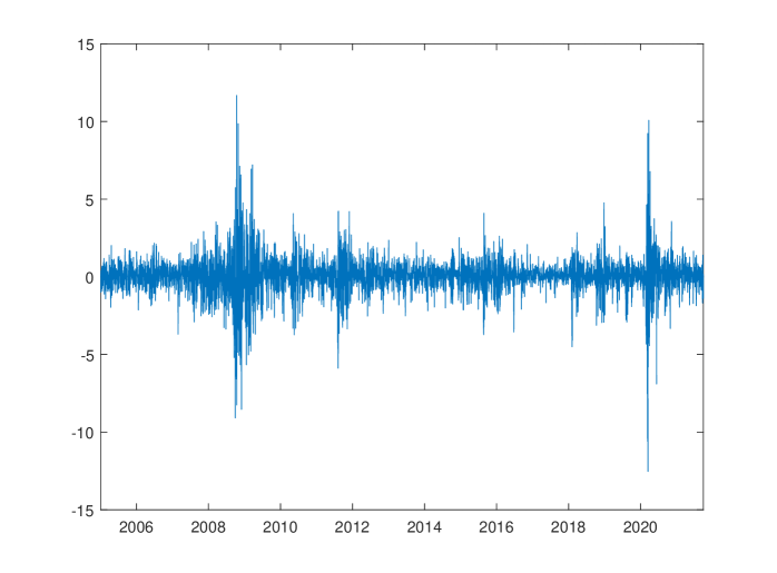
Figure 1: Equally weighted portfolio returns for 28 assets in the Dow Jones index.

A rolling window scheme, with fixed in-sample size $T_{\text{in}}=3000$ and daily re-estimation, is then implemented to generate $T_{\text{out}}=1213$ out-of-sample one-step-ahead forecasts of VaR and ES at 2.5% level. Therefore, the in-sample period is from 4 January 2005 to 1 December 2016, and the out-of-sample period covers the time range from 2 December 2016 to 28 September 2021.

Several existing univariate semi-parametric models are selected as benchmarks for comparison. First, we consider the recently proposed ES-CAViaR model (Taylor, 2019) with Symmetric Absolute Value (SAV) and Indirect GARCH (IG) specifications for the quantile regression equation. Regarding the ES specification, to facilitate the performance comparison with the DCC-AL, we choose the model with the constant multiplicative ES to VaR factor $(1+\text{exp}(\gamma_{0}))$, which is the factor that we use in the proposed DCC-AL model.

In addition, the semi-parametric Conditional Autoregressive Expectile framework (CARE, Taylor 2008), with SAV and IG specifications, is also included.

Furthermore, the risk forecasting performances of the proposed framework are compared to those yielded by the conventional DCC models fitted through different estimation approaches. First, we consider a standard DCC model fitted by a two-stage procedure (Engle, 2002) combining maximization of Gaussian likelihoods in the first (volatility) and second (correlation) stages of the estimation procedure with the application of correlation targeting. At the VaR and ES forecasting stage, depending on the assumptions formulated on the error distribution, two different series of forecasts are generated and labeled as DCC-N, when a multivariate Normal distribution is assumed, and DCC-QML, when a semi-parametric approach is taken. Namely, for the DCC-N approach, the theoretical quantile and tail expectation based on the Normal distribution are used for VaR and ES calculation. For the QML, differently, the semi-parametric filtered historical simulation approach is used to calculate the VaR and ES. The error quantiles $\hat{q}$ and tail expectations $\hat{c}$ are then estimated by computing the relevant sample quantiles and tail averages of standardized returns ($r_{t}$ divided by its volatility). Finally, level-$\alpha$ VaR and ES forecasts are obtained by multiplying $\hat{q}$ and $\hat{c}$, respectively, by the portfolio conditional standard deviation forecast from the fitted DCC model.

When applied to even moderately large datasets, such as the one that is here considered, the original approach to the estimation of DCC parameters described in Engle (2002) has been found to be prone to return biased estimates of the correlation dynamic parameters. This motivates our choice to consider, as a further benchmark, the Composite Likelihood (clik) approach developed in Pakel et al. (2021). Along the same lines discussed above, the estimated volatility and correlation parameters are then used to generate two different sets of VaR and ES forecasts labeled as DCC-clik-N and DCC-clik-QML, respectively.

Finally, the picture is completed by considering a parametric DCC model fitted by ML using multivariate Student’s $t$ likelihoods in the estimation of volatility and correlation parameters (DCC-t). VaR and ES forecasts are generated considering theoretical quantiles and tail expectations for a standardized Student’s $t$ distribution.

For all the DCC benchmarks, in order to guarantee a fair comparison with the DCC-AL model, the fitted univariate volatility specifications are given by GARCH(1,1) models.

In Figure (2), it is interesting to note that the estimated correlation parameters in the DCC-AL model vary over the forecasting period, reacting to changes in the underlying market volatility level. In particular, the estimated value of $a$ is characterized by a positive trend originating at the outbreak of the pandemic COVID-19 crisis. An opposite behaviour is observed for $b$.

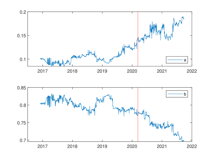
Figure 2: Plots of estimated correlation parameters $a$ and $b$ of the DCC-AL model. The vertical lines denote the outbreak of the COVID-19 emergency (as officially declared by the World Health Organization on 30 January 2020). Whole forecasting sample (1213 days).

Table 1 compares the DCC-AL estimates of correlation coefficients with those obtained for the benchmark DCC specifications considered, reporting the average estimates of correlation parameters $a$ and $b$ across all forecasting steps. Here, consistent with previous findings in the literature, standard DCC estimators tend to oversmooth (estimated $b$ very close to 1) correlations, while this is not the case for DCC-AL models. The DCC-clik estimates stay in between. It is here worth noting that the DCC-clik and DCC-AL models are based on different first stage volatility estimators: QML-GARCH for DCC-clik, and ES-CAViaR-IG as in Equation (6) for DCC-AL. In addition, Figure 3 shows the cross-sectional averages of the estimated conditional correlations (calculated based on $P_{t}$ in Equation (11)) across the forecasting period. As can be seen, the dynamics of the estimated conditional correlations between DCC-AL and DCC-clik are relatively close to each other.

Table 1: Average estimates (across time) of correlation dynamic parameters ($a$ and $b$) from different models and estimation methods. Whole forecasting sample (1213 days).

	DCC-AL	DCC-QML	DCC-t	DCC-clik
$a$	0.1217	0.0040	0.0023	0.0308
$b$	0.7827	0.9788	0.9816	0.9198

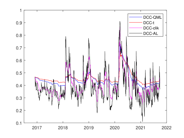
Figure 3: Cross-sectional averages of the estimated conditional correlation for DCC-QML, DCC-t, DCC-clik and DCC-AL across the whole forecasting sample (1213 days).

The average of estimated first stage univariate modelling coefficients, across all assets and forecasting steps, is reported in Table 2. GARCH-$t$ and QML-GARCH, used in DCC-t and DCC-QML respectively, appear to be less reactive (smaller $\alpha$ estimates) to past shocks compared to the ES-CAViaR-IG, used in the DCC-AL model.

Table 2: Average estimates (across times and assets) of the first stage univariate modelling parameters ($\alpha$ and $\beta$) from different models and estimation methods across the full forecasting sample (1213 days). For ES-CAVIAR-IG, we report $\alpha=\alpha^{(q)}/q^{2}$.

	GARCH-$t$	QML-GARCH	ES-CAViaR-IG
$\alpha$	0.0902	0.0852	0.1369
$\beta$	0.8702	0.8944	0.8059

5.2 Evaluation of VaR and ES forecasts

Assuming equally weighted portfolio returns, one-step-ahead forecasts of daily VaR and ES from the proposed DCC-AL model are produced by using Equation (14). In this section, these forecasts are compared with the ones from the competing models presented in Section 5.1.

The standard quantile loss function is employed to compare the models for VaR forecast accuracy: the most accurate VaR forecasts should minimize the quantile loss function, given as:

$$\sum_{t=T_{\text{in}}+1}^{T_{\text{in}}+T_{\text{out}}}(r_{t}-\widehat{Q}_{t})(\alpha-I(r_{t}\leq\widehat{Q}_{t}))\,\,,$$ (18)

where $T_{\text{in}}$ is the in-sample size, $T_{\text{out}}$ is the out-of-sample size and $\widehat{Q}_{T_{\text{in}}+1},\ldots,\widehat{Q}_{T_{\text{in}}+T_{\text{out}}}$ is a series of VaR forecasts at level $\alpha$ for observations $r_{T_{\text{in}}+1},$ $\ldots,$ $r_{T_{\text{in}}+T_{\text{out}}}$.

Moving to the assessment of joint (VaR, ES) forecasts, as discussed in Section 2.2, Taylor (2019) shows that the negative logarithm of the likelihood function built from Equation (4) is strictly consistent for $Q_{t}$ and $\text{ES}_{t}$ considered jointly, and fits into the class of strictly consistent joint loss functions for VaR and ES developed by Fissler and Ziegel (2016). This loss function is also called the AL log-score in Taylor (2019) and is defined as:

$$S_{t}(r_{t},\widehat{Q}_{t},\widehat{\text{ES}}_{t})=-\text{log}\left(\frac{\alpha-1}{\widehat{\text{ES}}_{t}}\right)-{\frac{(r_{t}-\widehat{Q}_{t})(\alpha-I(r_{t}\leq\widehat{Q}_{t}))}{\alpha\widehat{\text{ES}}_{t}}}.$$ (19)

In our analysis, we use the joint loss $S=\sum_{t=T_{\text{in}}+1}^{T_{\text{in}}+T_{\text{out}}}S_{t}$ to formally and jointly assess and compare the VaR and ES forecasts from all models.

Figure 4 visualizes the 2.5% portfolio ES forecasts from the DCC-QML, DCC-clik-QML and DCC-AL models for the Jan 2019–Sep 2021 period, using equally weighted Dow Jones returns. In general, we can see that the ES forecasts produced from the DCC-AL model have a long-run behaviour comparable to the ones from the DCC-QML and DCC-clik-QML. However, in the short term, forecasts from these models can be characterized by substantially different dynamic patterns. This is particularly evident in the period immediately following the outbreak of the COVID-19. Inspecting the ES forecasts at the beginning of 2020, we can see that the three models have distinctive behaviours. Comparing to the DCC-QML model, the DCC-AL model is more reactive to the return shocks. This is because of the larger $a$ and $\alpha$ estimates as discussed in Tables 1 and 2. The ES forecasts from the DCC-clik-QML stay in between the ones from DCC-QML and DCC-AL, which is also consistent with the findings from Table 1.

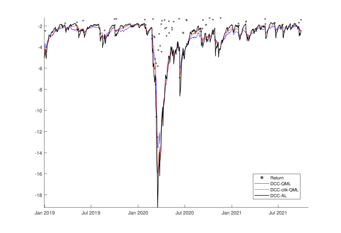
Figure 4: 2.5% ES forecasts from the DCC-QML, DCC-clik-QML and DCC-AL models, using equally weighted Dow Jones returns.

The quantile and joint loss results from the proposed DCC-AL model and other competing models are shown in Table 3. Overall, the results show that the proposed DCC-AL model, in comparison to the other models under analysis, generates competitive loss results, which lends evidence on the validity of the proposed semi-parametric framework. Furthermore, the DCC-AL model generates smaller loss values than all other parametric or semi-parametric DCC models that have been taken as benchmarks.

The Model Confidence Set (MCS) of Hansen et al. (2011) is employed to statistically compare the quantile loss (Equation (18)) and joint loss (Equation (19)) values yielded by the different models. A MCS is a set of models, constructed such that it contains the best model with a given level of confidence, selected as either 75% or 90% in our paper. Two methods, R and SQ (see Hansen et al., 2011, for details), are employed to calculate the MCS test statistic. The MCS results, using both quantile and joint loss functions, are shown in Table 4. As can be seen, the DCC-AL is included in the MCS for both methods across both 90% and 75% tests. However, the DCC-QML, DCC-N and DCC-clik-N models are excluded from the 90% MCS with the SQ method and joint loss. On the 75% level with the SQ method and joint loss, all the DCC models, except the proposed DCC-AL, are excluded from the MCS.

Table 3: The quantile loss (Equation (18)) and joint loss function (Equation (19)) values for all competing models across the full forecasting sample.

Model	Quantile loss	Joint loss
CARE-SAV	90.4	2,405.4
CARE-IG	89.1	2,392.1
ES-CAViaR-SAV	89.4	2,398.1
ES-CAViaR-IG	87.3	2,369.5
DCC-QML	98.7	2,492.6
DCC-N	101.2	2,566.8
DCC-clik-QML	95.2	2,453.9
DCC-clik-N	97.7	2,528.9
DCC-t	101.5	2,555.3
DCC-AL	89.1	2,386.8

Table 4: The 90% and 75% MCS results based on the quantile loss and joint loss function values, using both the R and SQ methods.

Model	R - quantile	SQ - quantile	R - joint	SQ - joint
90% MCS
CARE-SAV	1	1	1	1
CARE-IG	1	1	1	1
ES-CAViaR-SAV	1	1	1	1
ES-CAViaR-IG	1	1	1	1
DCC-QML	1	1	1	0
DCC-N	1	1	1	0
DCC-clik-QML	1	1	1	1
DCC-clik-N	1	1	1	0
DCC-t	1	1	1	1
DCC-AL	1	1	1	1
75% MCS
CARE-SAV	1	1	1	1
CARE-IG	1	1	1	1
ES-CAViaR-SAV	1	1	1	1
ES-CAViaR-IG	1	1	1	1
DCC-QML	1	1	1	0
DCC-N	1	1	1	0
DCC-clik-QML	1	0	1	0
DCC-clik-N	1	0	1	0
DCC-t	1	1	1	0
DCC-AL	1	1	1	1

Note:“0” in red represents models that are not in MCS.

To further backtest the VaR forecasts, we have employed several quantile accuracy and independence tests, including: the unconditional coverage (UC) test (Kupiec et al., 1995); the conditional coverage (CC) test (Christoffersen, 1998); the dynamic quantile (DQ) test (Engle and Manganelli, 2004); and the quantile regression based VaR (VQR) test (Gaglianone et al., 2011). Table 5 presents the UC, CC, DQ (lag 1 and lag 4) and VQR backtests’ p-values for the 10 competing models. The “Total” columns show the total number of rejections at the 5% significance level. As can be seen, the DCC-AL is the only framework which receives 0 rejections. The DCC-N model receives 5 rejections, while the DCC-t model gets rejected 3 times. This demonstrates the importance of the return distribution selection in parametric MGARCH models. The DCC-AL model, which is semi-parametric, shows advantage from this perspective. Comparing the DCC-AL model to the semi-parametric DCC models with QML, the DCC-AL still has better performance considering these backtests. These results again lend evidence on the validity and effectiveness of the DCC-AL in forecasting VaR.

Table 5: Summary of 2.5% VaR forecasts UC, CC, DQ1, DQ4, and VQR backtests’ p-values and the total number of rejections at the 5% significance level.

Model	UC	CC	DQ1	DQ4	VQR	Total
CARE-SAV	76%	16%	9%	3%	46%	1
CARE-IG	95%	46%	41%	6%	0%	1
ES-CAViaR-SAV	90%	14%	8%	2%	68%	1
ES-CAViaR-IG	67%	83%	82%	1%	84%	1
DCC-QML	76%	3%	0%	0%	0%	4
DCC-N	4%	2%	0%	0%	0%	5
DCC-clik-QML	51%	18%	6%	0%	20%	1
DCC-clik-N	9%	10%	4%	0%	5%	2
DCC-t	13%	4%	0%	0%	11%	3
DCC-AL	67%	83%	81%	8%	42%	0

Lastly, Bayer and Dimitriadis (2022) propose three versions of ES backtests named as Auxiliary, Strict and Intercept ES regression (ESR) backtests. These ESR backtests (two-sided), labeled as A, S, and I respectively, are also employed to backtest the ES forecasts from the 10 competing models.

As in Table 6, the three backtests return quite consistent results, with the DCC-AL model being not rejected. The models that get rejected at the 5% level by all three backtests are DCC-N, DCC-clik-N and DCC-t. Meanwhile, the semi-parametric DCC-QML and DCC-clik-QML do not get rejected.

Table 6: Summary of three versions (A, S, I) of ES backtests’ p-values and the total number of rejections at the 5% significance level.

Model	A	S	I	Total
CARE-SAV	83%	83%	70%	0
CARE-IG	95%	95%	76%	0
ES-CAViaR-Mult-SAV	92%	92%	78%	0
ES-CAViaR-IG	96%	96%	96%	0
DCC-QML	20%	20%	24%	0
DCC-N	0%	0%	1%	3
DCC-clik-QML	35%	35%	21%	0
DCC-clik-N	0%	0%	1%	3
DCC-t	2%	2%	1%	3
DCC-AL	87%	87%	71%	0

5.3 Hedging performance

In this section we evaluate the hedging performance of the DCC-AL model in producing minimum variance, 2.5% VaR and ES portfolios and compare results with those obtained by standard DCC models taken as benchmarks. Minimum risk (VaR and ES) portfolios are computed using the PO procedure illustrated in Section 4 with the main difference that, since our interest is in hedging, at this stage we do not impose any constraint on the target mean return $\mu_{0}$ of the optimized portfolio. On the other hand, minimum variance portfolios are, as usual, computed by numerically minimizing portfolio volatility with respect to the weights vector $\mathbf{w}$.

First, we present some empirical results to further demonstrate how the PO procedure proposed in Section 4 works and lend evidence on its validity.

In particular, Figure 8 reports the time series of the out-of-sample OLS predicted VaR and ES factors at the optimum, $\mathbf{w}^{{}^{\prime}}_{q,opt}\widehat{\bm{\beta}}_{q}$ and $\mathbf{w}^{{}^{\prime}}_{c,opt}\widehat{\bm{\beta}}_{c}$, obtained through the OLS regression embedded in Step 4 of the procedure, and compares them with the estimated VaR and ES factors at the minimum risk portfolios, i.e., for $\mathbf{w}=\mathbf{w}_{q,opt}$ and $\mathbf{w}=\mathbf{w}_{c,opt}$ respectively. The latter are obtained as follows: relying on the out-of-sample optimized minimum VaR and ES portfolio weights, at each forecasting step we re-estimate the DCC-AL model on the optimized portfolio returns, thus obtaining a new set of estimates for the underlying VaR and ES factors that we denote as $\hat{q}_{\alpha}(\mathbf{w}_{q,opt})$ and $\hat{c}_{\alpha}(\mathbf{w}_{c,opt})$, respectively. Being based on the minimization of a strictly consistent loss, under correct specification of the underlying risk dynamics, $\hat{q}_{\alpha}(\mathbf{w}_{q,opt})$ and $\hat{c}_{\alpha}(\mathbf{w}_{c,opt})$ provide consistent estimates for the underlying $q_{\alpha}(\mathbf{w}_{opt})$ and $c_{\alpha}(\mathbf{w}_{opt})$. Hence, a comparison of these estimates with the OLS predictions at the optimum can be used to check the accuracy of the latter approximation for the risk factors of the optimized portfolios. It is evident that the OLS predicted VaR factors and estimated $\hat{q}_{\alpha}(\mathbf{w}_{q,opt})$ series are very close. Similar observations hold for ES. Therefore, such results provide encouraging evidence in favour of the validity of the PO procedure which can produce estimated VaR and ES factors that approximate the underlying values with good accuracy. In this way, the PO procedure, while still not assuming ellipticity, avoids the re-estimation of the DCC-AL model at each PO iteration.

Figure 5: The top plot shows the OLS predicted VaR factor $\mathbf{w}^{{}^{\prime}}_{q,opt}\widehat{\bm{\beta}}_{q}$ and the estimated $\hat{q}_{\alpha}(\mathbf{w}_{q,opt})$ in DCC-AL for the optimized minimum VaR portfolio. The bottom plot shows the OLS predicted ES factor $\mathbf{w}^{{}^{\prime}}_{c,opt}\widehat{\bm{\beta}}_{c}$ and the estimated $\hat{c}_{\alpha}(\mathbf{w}_{c,opt})$ in DCC-AL for the optimized minimum ES portfolio. Whole forecasting sample (1213 days).

Next, we focus on the assessment of the out-of-sample hedging performance of the DCC-AL model and the other benchmark DCC specifications considered in the analysis.

A summary of the PO optimization results is shown in Tables 7. The top section focuses on the whole out-of-sample period. The bottom section studies a forecasting subsample including 100 consecutive days, from 7 February 2020 to 1 July 2020, in a neighbourhood of the COVID-19 outbreak.

Table 7: Descriptive statistics of out-of-sample returns $r^{(p)}_{t}$ for different portfolios with $\alpha=2.5\%$. $\widehat{\mathbb{V}}(r^{(p)}_{t})$: empirical variance; $\widehat{VaR}(r^{(p)}_{t},\alpha)$: empirical VaR; $\widehat{ES}(r^{(p)}_{t},\alpha)$: empirical ES. The top section corresponds to the whole forecasting sample (1213 days). The bottom section corresponds to the forecasting steps 801-900 (100 days from 7 February 2020 to 1 July 2020).

	$\widehat{\mathbb{V}}(r^{(p)}_{t})$	$\widehat{VaR}(r^{(p)}_{t},\alpha)$	$\widehat{ES}(r^{(p)}_{t},\alpha)$
Whole forecasting sample (1213 days)
EW	1.5233	- 2.4682	- 4.1951
DCC-QML min. variance	1.0342	- 2.0135	- 3.6360
DCC-t min. variance	1.0310	- 1.9407	- 3.5127
DCC-QML min. VaR	1.0001	- 1.9722	- 3.5255
DCC-QML min. ES	1.0262	- 1.9953	- 3.5928
DCC-clik-QML min. variance	0.9788	- 1.9517	-3.2625
DCC-clik-QML min. VaR	0.9844	- 1.9992	- 3.3384
DCC-clik-QML min. ES	0.9818	- 1.9755	- 3.3407
DCC-AL min. variance	1.0037	- 2.0884	- 3.5945
DCC-AL min. VaR	0.9841	- 2.1251	- 3.5503
DCC-AL min. ES	0.9840	- 2.1077	- 3.5534
“COVID-19” subsample (100 days)
EW	11.2036	- 7.5400	- 11.5660
DCC-QML min. variance	6.6620	- 6.3077	- 9.3131
DCC-t min. variance	6.5782	- 6.4684	- 9.7652
DCC-QML min. VaR	6.3404	- 5.4028	- 9.1153
DCC-QML min. ES	6.5718	- 5.9916	- 9.3512
DCC-clik-QML min. variance	6.0174	- 5.9946	-7.0825
DCC-clik-QML min. VaR	6.0992	- 6.8327	- 7.2388
DCC-clik-QML min. ES	6.0821	- 6.7658	- 7.1063
DCC-AL min. variance	6.0097	- 5.9419	- 7.0825
DCC-AL min. VaR	5.8914	- 6.3003	- 7.0356
DCC-AL min. ES	5.8973	- 6.2114	- 7.1063

For all the competing models, including DCC-QML, DCC-t, DCC-clik-QML and the proposed DCC-AL, the minimum variance portfolios are firstly calculated. Then, for the same models we report results for minimum risk portfolios.

It is here worth making some preliminary considerations. For DCC-t and DCC-N, due to the spherical nature of the chosen error distribution, minimum variance and minimum risk hedged portfolios are virtually identical. Furthermore, DCC-(clik)-QML and DCC-(clik)-N by construction return identical minimum variance allocations, being based on the same estimated conditional variance and covariance matrix.

For all models, minimum VaR and ES portfolios are computed using the PO procedure in Section 4. In Table 7, the labels model A min. variance, model A min. VaR and model A min. ES denote minimum variance, VaR and ES portfolios, respectively, generated from model A.

The portfolio allocation exercise is based on the same rolling window scheme described in Section 5.2. At each time point $t$, models are estimated on a rolling window of 3000 observations extending up to time $t$ and the predicted $\widehat{H}_{t+1}$ is used to optimize portfolio allocation for time $t+1$. We rule out short-selling operations by restricting portfolio weights to take values in [0,1].

As measures of hedging performance we report the out-of-sample empirical variances, VaR and ES computed over the hedged portfolios for the different models. Lastly, an equally weighted (EW) portfolio is included as a benchmark.

Compared to the benchmark EW case, all the estimated DCC models yield substantial reductions in terms of out-of-sample empirical variance, VaR and ES. When focusing on the whole out-of-sample period (top section in Table 7), the DCC models under analysis return quite similar hedging performances.

On the other hand, more relevant differences appear in a short term perspective when focusing on the period immediately following the COVID-19 outbreak (bottom section in Table 7). Although we are aware that one should be cautious in the evaluation of performance rankings based on such a short forecast subsample, an important merit of this short-term analysis is to offer an empirical appraisal of the extent to which minimum variance and minimum risk allocations can differ in high volatility periods.

Compared to the empirical findings arising for the whole forecasting period, our results show that DCC-AL and DCC-clik-QML models are able to hedge ES risk more effectively than DCC-QML and DCC-t. For example, the empirical $\widehat{ES}(r^{(p)}_{t},\alpha)$ produced by the DCC-AL and DCC-clik-QML minimum ES portfolios are (in absolute values) smaller than that of the DCC-QML and DCC-t. Comparing the DCC-AL and DCC-clik-QML models, we find that the two models return close performances. The empirical variance $\widehat{\mathbb{V}}(r^{(p)}_{t})$ of the DCC-AL minimum variance portfolio is very close to that of the DCC-clik-QML minimum variance portfolio, while both approaches return out-of-sample empirical portfolio variances that are lower than those yielded by other DCC specifications. When comparing the minimum VaR portfolios produced by the DCC-AL and DCC-clik-QML, we note that the empirical VaR from DCC-AL is, in absolute value, smaller although, for this forecast subsample, the best performance is surprisingly returned by the DCC-QML minimum VaR portolio.

The empirical ES values from DCC-AL and DCC-clik-QML minimum VaR portfolios are identical.

Summarizing the empirical evidence, what we have found is that in the long-term, when referring to the whole forecasting period, the selected performance indicators, based on unconditional variance, VaR and ES, do not reveal any striking differences between minimum variance and minimum risk portfolios. This suggests that the conditional distribution of returns is, for most days, likely to be close to some distribution falling within the elliptical family.

Nevertheless, in the short term, the selected optimal portfolio allocations can differ quite substantially across different strategies: that is minimum variance, VaR and ES. Evidence in this direction is indirectly provided by the analysis performed on the 100 days “COVID-19” subsample. More specifically, Figure 6, which reports differences between asset allocations yielded by minimum variance and minimum risk portfolios for the 100 days “COVID-19” subsample, confirms this intuition. Even if the median differences tend to stay close to zero, the tails of the boxplots reveal that there are more than a few time periods in which the weights assigned to specific portfolio assets can differ quite a lot across different allocation strategies.

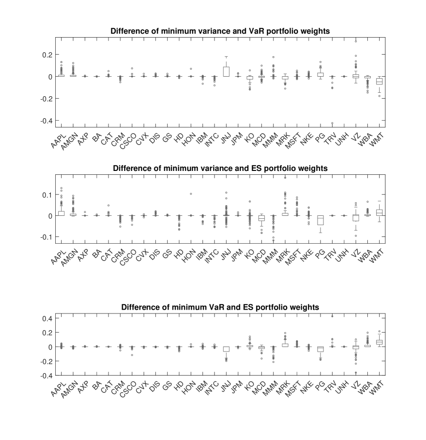
Figure 6: Boxplots of differences of DCC-AL model minimum variance and VaR, minimum variance and ES, and minimum VaR and ES portfolio weights. The x-axis shows the 28 components of the Dow Jones index. Period: forecasting steps 801-900 (100 days) corresponding to the interval 7 February 2020 to 1 July 2020..

6 Conclusions

In this paper, we propose an innovative framework for forecasting portfolio tail risk in a multivariate and semi-parametric setting. The proposed framework is capable of modelling high dimensional return series parsimoniously and efficiently. In addition, a statistical procedure is designed to employ the proposed framework for optimising the portfolio VaR and ES. Compared to the state-of-the-art univariate semi-parametric models, the proposed framework delivers competitive risk forecasting performances and, in addition, it can be used for a wider range of applications including portfolio optimization. Compared to existing DCC estimation approaches, our empirical application shows that the DCC-AL is able to deliver more accurate risk forecasts and hedging performances in line with those of DCC-clik-QML estimators (Pakel et al., 2021).

From a different viewpoint, it is worth noting that our framework also delivers a semi-parametric approach to the generation of robust estimates of DCC coefficients. Under this respect, in our empirical application we find that semi-parametric estimates of dynamic correlation parameters obtained from the DCC-AL model, as the DCC-clik estimator, are potentially not affected by the well known severe downward bias towards zero that, in even moderately large dimensions, typically characterizes estimates obtained through Gaussian QML (Pakel et al., 2021). A comparison of the statistical properties of our estimator with those of QML and clik-QML would be of great interest. However, this goes beyond the scope of this paper and is currently left for future research.

In addition to this, our projects for future research are focused on two main additional issues. First, we are extending the DCC-AL model via including high frequency realized measures, to further improve its performance. A second issue of interest is related to a refinement of the minimum risk PO procedure discussed in Section 4. In particular, the OLS regression in Step 4 of the procedure could be replaced with a more parsimonious penalized regression (e.g., LASSO) or a more flexible Neural Network regression. This issue is currently under investigation in a separate project.

Appendix A

Simulation study

A simulation study has been conducted in order to assess the statistical properties of the two-step AL loss based estimation procedure discussed in Section 3. In this Appendix we provide a detailed description of the simulation design and of the main findings of our study.

Our analysis has two main objectives. First, the study evaluates the bias and efficiency of the estimators of the DCC-AL parameters ($a,b,q,\gamma_{0}$). Second, we also assess the the risk forecasting performances of the estimated DCC-AL model in an equally weighted portfolio, via comparing the one-step-ahead $2.5\%$ level portfolio VaR and ES forecast accuracy to the “true” simulated values.

In line with the empirical findings arising from our empirical application, we have considered the Data Generating Process (DGP) as a parametric DCC model of dimension $n$=28 with the true values of the correlation dynamic parameters in Equation (13) given by $a=0.12$ and $b=0.78$:

$$Q_{t}=(1-0.12-0.78)\Sigma_{\bm{\epsilon}}+0.12\bm{\epsilon}_{t-1}\bm{\epsilon}^{{}^{\prime}}_{t-1}+0.78Q_{t-1},$$ (20)

where $\Sigma_{\bm{\epsilon}}$ is a $n\times n$ matrix with unit diagonal and off-diagonal elements equal to 0.5.

In the return equation $\mathbf{r}_{t}=\bm{\mu}_{t}+H^{1/2}_{t}\mathbf{z}_{t}$, the conditional mean vector $\bm{\mu}_{t}$ of returns is chosen to be zero. The DGP univariate volatilities are assumed to follow the GARCH(1,1) model:

$$h^{2}_{t,i}=0.1+0.1r^{2}_{t-1,i}+0.8h^{2}_{t-1,i},\qquad i=1,\ldots,n.$$

The parametric distribution of returns is assumed to be $\mathbf{z}_{t}\overset{iid}{\sim}D_{1}(\mathbf{0},I_{n})$, where the following choices of $D_{1}$ have been considered:

• Standardized multivariate Normal distribution: $\mathbf{z}_{t}\overset{iid}{\sim}\mathcal{N}_{n}(\mathbf{0},I_{n})$.

• Standardized multivariate Student’s $t$ distribution: $\mathbf{z}_{t}\overset{iid}{\sim}t_{n}(\mathbf{0},I_{n};\nu)$, where the degrees of freedom parameter $\nu$ has been set equal to 10.

• A multivariate non-spherical distribution with Student’s $t$ marginals ($nst$: $\mathbf{z}_{t}\overset{iid}{\sim}nst_{n}(\mathbf{0},I_{n};\bm{\nu})$; the density of this distribution is obtained taking the product of $n$ independent univariate standardized $t_{1}(0,1;{\nu}_{i})$ densities; $\bm{\nu}=(\nu_{1},\ldots,\nu_{n})$ is the $n$-dimensional vector of marginal degrees of freedom parameters. When $\nu_{i}=\nu$ ($\forall i$), the marginal densities of the product are the same as those of the multivariate $t$, although the joint density is different (Bauwens and Laurent, 2005). In our simulations, the values of $\nu_{i}$ have been uniformly drawn over the interval [5,15].

While the first two distributions belong to the spherical family, the same does not hold for the third one ($nst$).

The DCC-AL model is then fitted to the time series of equally weighted $(\mathbf{w}=1/n)$ portfolio returns generated from the chosen DGP, for three different sample sizes $T\in\{2000,3000,5000\}$. Overall, matching 3 different distributional assumptions and sample sizes, we have 9 simulation settings and, under each of these, 250 return series have been generated.

Conditional on the chosen error distribution and on the values of the correlation parameters $a$ and $b$, the true values of the other two parameters $q$ and $\gamma_{0}$ in the DCC-AL model can be then calculated as follows.

In the spherical case, multivariate Normal and $t$, letting $F(.)$ be the CDF of $z_{t,i}$, $q=F^{-1}(\alpha)$ and $c=E(z_{t,i}|z_{t,i}\leq q)$. By Equation (15) it is then easy to obtain:

$$\gamma_{0}=\log\left(\frac{c^{2}}{q^{2}}-1\right).$$

Therefore, taking the multivariate Normal case as an example, in the DCC-AL the true value of $q^{2}$ is $\Phi^{-1}(\alpha)^{2}=(-1.96)^{2}=3.8415$. The true value for $c^{2}$ is $\left(\frac{\phi(\Phi^{-1}(\alpha))}{\alpha}\right)^{2}=(-2.3378)^{2}$, where $\Phi$ is the standard Normal CDF and $\phi$ is standard Normal Probability Density Function (PDF). Further, we have $(1+\text{exp}(\gamma_{0}))=\frac{c^{2}}{q^{2}}=\frac{(-2.3378)^{2}}{(-1.9600)^{2}}=1.4227$, thus $\gamma_{0}=\text{log}(1.4227-1)=-0.8610$. These true values of $a$, $b$, $\gamma_{0}$ and $q^{2}$ for the multivariate Normal distribution are shown in the True rows in Table 8. When $\mathbf{z}_{t}\overset{iid}{\sim}t_{n}(\mathbf{0},I_{n};\nu=10)$, the true values of $q$, $c$ and $\gamma_{0}$ are obtained through a similar approach, replacing the analytical formulas for $q$ and $c$ with the equivalent expressions for an univariate $t$ distribution.

In the $nst$ case, the true values of $q$, $c$ and $\gamma_{0}$ need to be calculated via simulations since this distribution is not a member of the spherical family. It also follows that, differently from what observed for the multivariate Normal and $t$ cases, the values of these coefficients will be dependent on the chosen portfolio allocation. So they could change when moving from equal weighting to a different allocation scheme.

More specifically, $q$ and $c$ can be calculated by the following procedure.

1. For a given set of randomly generated degrees of freedom values $\bm{\nu}$ and portfolio allocation $\mathbf{w}$, a return series with size $T_{sim}\times n$ ($T_{sim}=10^{5}$) is simulated from the specific DCC process taken as DGP: $\mathbf{r}^{*}_{j}$, $j=1,\ldots,T_{sim}$.

2. Given the simulated returns vector $\mathbf{r}^{*}_{j}$, conditional covariance matrix ${H}^{*}_{j}$ and portfolio allocation $\mathbf{w}$, the time series of simulated standardized portfolio returns is computed as:

   $$z^{*}_{j}=\frac{r^{*}_{j}}{h^{*}_{j}},$$

   for $j=1,\ldots,T_{sim}$ and where

   $$r^{*}_{j}=\mathbf{w}^{\prime}\mathbf{r^{*}_{j}},\qquad h^{*}_{j}=\sqrt{\mathbf{w}^{\prime}{H}^{*}_{j}\mathbf{w}}.$$

3. The empirical quantile and conditional tail average of the $z^{*}_{j}$ series are then used as the simulated “true” values for $q$ and $c$. These values can be used to calculate the true values for $\gamma_{0}$ through inverting Equation (15).

For ease of reference, for each DGP, the true parameter values for $(a,b,q,\gamma_{0})$ are included in the True rows in Table 8.

The DCC-AL model is then fitted to each simulated dataset, using the estimation procedure as outlined in Section 3. The simulation results for the DCC-AL model are shown in Table 8 where, for ease of presentation, we have chosen not to report parameter estimates of the fitted first stage ES-CAViaR-IG models.

The rows labeled as True report, for each DGP, the values of the parameter true values used for simulation. The empirical averages of the 250 parameter estimates, for various return distributions and sample sizes, are shown in the Mean rows. The Root Mean Squared Error (RMSE) values between the parameter estimates and the true values are shown in the RMSE rows in Table 8.

To further evaluate the accuracy of the portfolio VaR and ES forecasts from the estimated DCC-AL model, for all 250 simulated datasets, we compare the one-step-ahead $\widehat{Q}_{T+1}$ and $\widehat{\text{ES}}_{T+1}$ forecasts based on the estimated parameters with their counterparts based on the true DGP coefficients. For $\widehat{Q}_{T+1}$ and $\widehat{\text{ES}}_{T+1}$, the True rows then report the averages of the 250 risk forecasts based on the true parameters, for different return distributions and sample sizes.

First, the results provide support to the use of the two-step AL based estimation method and show that it is able to produce relatively accurate parameter estimates. Overall, the estimated bias ($|\emph{Mean}-\emph{True}|$) is reasonably low. When the distribution is fixed, the absolute bias decreases as the time series length $T$ increases. For all parameters, the values of the RMSE also monotonically decrease as $T$ increases, suggesting consistency of the estimation procedure. When the sample size is fixed, as expected, the RMSE values are clearly larger when the errors follow a multivariate Student’s $t$, comparing to multivariate Normal distribution.

The estimation results are still relatively accurate for the non-spherical $nst$ distribution that, for correlation parameters, returns RMSE values slightly higher than those obtained in the Normal case. For parameters $q$ and $\gamma_{0}$, the simulated RMSE is in line with the Normal case, for $\gamma_{0}$, and even lower for $q$.

These results suggest that the proposed semi-parametric estimation procedure is able not only to keep track of the volatility and correlation dynamics but also of the distributional properties of portfolio returns, through the estimation of $q$ and $\gamma_{0}$ (implicitly $c$).

Finally, reminding that the main motivation for the DCC-AL model is the generation of accurate portfolio risk forecasts, the last two columns of Table 8 provide a very important benchmark for assessing the properties of the proposed estimation procedure. Comparing the $\alpha=2.5\%$ estimated and true risk forecasts, for both VaR and ES, it can be noted that these two series are on average very close even for the shortest sample size $T=2000$. The RMSE values are also remarkably low: with $T=2000$ they do not exceed 0.0811 for VaR and 0.1034 for ES, and their values monotonically decrease as $T$ increases across three return distributions. This last set of results confirms the ability of the proposed two-stage estimation procedure to accurately reproduce the portfolio risk dynamics.

Table 8: DCC-AL model parameter estimates and VaR and ES forecasting results with simulated datasets.

DGP		$a$	$b$	$\gamma_{0}$	$q^{2}$	$\widehat{Q}_{T+1}$	$\widehat{\text{ES}}_{T+1}$
$\mathcal{N}$, $T=2000$	True	0.1200	0.7800	-0.8610	3.8415	-1.3704	-1.6346
	Mean	0.1360	0.7150	-0.9131	3.9308	-1.3849	-1.6420
	RMSE	0.0751	0.1995	0.1639	0.2057	0.0606	0.0762
$\mathcal{N}$, $T=3000$	True	0.1200	0.7800	-0.8610	3.8415	-1.3565	-1.6180
	Mean	0.1310	0.7319	-0.8919	3.9079	-1.3669	-1.6244
	RMSE	0.0615	0.1736	0.1200	0.1613	0.0521	0.0611
$\mathcal{N}$, $T=5000$	True	0.1200	0.7800	-0.8610	3.8415	-1.3665	-1.6299
	Mean	0.1265	0.7528	-0.8830	3.9018	-1.3760	-1.6367
	RMSE	0.0466	0.1118	0.1029	0.1363	0.0392	0.0454
$t$, $T=2000$	True	0.1200	0.7800	-0.5097	3.9717	-1.4353	-1.8159
	Mean	0.1591	0.6719	-0.5844	4.1136	-1.4479	-1.8108
	RMSE	0.1023	0.2419	0.1894	0.2967	0.0811	0.1034
$t$, $T=3000$	True	0.1200	0.7800	-0.5097	3.9717	-1.3825	-1.7491
	Mean	0.1497	0.6894	-0.5658	4.0686	-1.3990	-1.7543
	RMSE	0.0884	0.2248	0.1527	0.2167	0.0692	0.0850
$t$, $T=5000$	True	0.1200	0.7800	-0.5097	3.9717	-1.4155	-1.7909
	Mean	0.1303	0.7395	-0.5459	4.0619	-1.4304	-1.7995
	RMSE	0.0617	0.1564	0.1172	0.1613	0.0534	0.0703
$nst$, $T=2000$	True	0.1200	0.7800	-0.8311	3.8772	-1.3570	-1.6259
	Mean	0.1440	0.7030	-0.8893	3.9012	-1.3538	-1.6096
	RMSE	0.0894	0.2245	0.1656	0.1849	0.0639	0.0762
$nst$, $T=3000$	True	0.1200	0.7800	-0.8311	3.8772	-1.3806	-1.6542
	Mean	0.1356	0.7223	-0.8657	3.8978	-1.3799	-1.6461
	RMSE	0.0729	0.1926	0.1246	0.1539	0.0576	0.0706
$nst$, $T=5000$	True	0.1200	0.7800	-0.8311	3.8772	-1.4001	-1.6775
	Mean	0.1277	0.7486	-0.8569	3.9091	-1.4057	-1.6788
	RMSE	0.0496	0.1195	0.1029	0.1251	0.0383	0.0465

2

Empirical support for the PO optimization procedure

In this section, we present some empirical results to demonstrate how the PO procedure proposed in Section 4 works and lend evidence on its validity. Figure 7 visualizes the simulated VaR and ES factors $\tilde{q}$ and $\tilde{c}$ (of size $N_{sim}\times 1$) generated from the in-sample data used for the first forecasting step. We can see that the simulated $\tilde{q}$ and $\tilde{c}$ series are centered around -2.1 and -2.7 respectively, with certain level of variation (noise) as expected. These two series are then used as dependent variables for the OLS Step 4 of the PO procedure. Figure 8 then reports the time series of the out-of-sample OLS predicted VaR and ES factors at the optimum ($\mathbf{w}^{{}^{\prime}}_{q,opt}\widehat{\bm{\beta}}_{q}$ and $\mathbf{w}^{{}^{\prime}}_{c,opt}\widehat{\bm{\beta}}_{c}$ as in Equation (17), obtained through the OLS regression embedded in Step 4 of the procedure, and compares them with the estimated VaR and ES factors at the minimum risk portfolios, i.e., $\mathbf{w}=\mathbf{w}_{q,opt}$ and $\mathbf{w}=\mathbf{w}_{c,opt}$. The latter is obtained as follows: relying on the out-of-sample optimized minimum VaR and ES portfolio weights, at each forecasting step we re-estimate the DCC-AL model on the optimized portfolio returns, thus obtaining a new set of estimates for the underlying VaR and ES factors that we denote as $\hat{q}(\mathbf{w}_{q,opt})$ and $\hat{c}(\mathbf{w}_{c,opt})$, respectively. Being based on the minimization of a strictly consistent loss, under correct specification of the underlying risk dynamics, $\hat{q}(\mathbf{w}_{q,opt})$ and $\hat{c}(\mathbf{w}_{c,opt})$ provide consistent estimates for the underlying $q(\mathbf{w}_{q,opt})$ and $c(\mathbf{w}_{c,opt})$. Hence, a comparison of these estimates with the OLS based predictions at the optimum can be used to check the accuracy of the latter approximation for the risk factors of the optimized portfolios. It is evident that the OLS predicted VaR factors and estimated $\hat{q}$ series are very close. Similar observations hold for ES. Therefore, such results demonstrate the validity of the PO procedure which can produce VaR and ES factors that can approximate the underlying $q$ and $c$ with good accuracy. In this way, the PO procedure, while still not assuming ellipticity, avoids the need of re-estimating the DCC-AL model at each portfolio configuration.

Figure 7: The simulated VaR and ES factors $\tilde{q}$ and $\tilde{c}$ of size $N_{sim}\times 1$ generated from the in-sample data used for the first forecasting step.

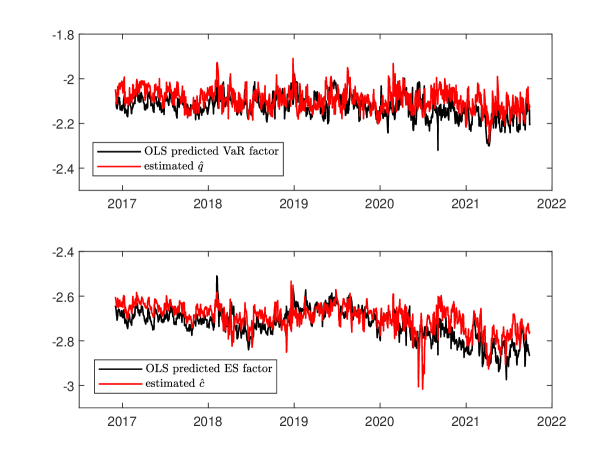
Figure 8: The top plot shows the OLS predicted VaR factor $\mathbf{w}^{{}^{\prime}}_{q,opt}\widehat{\bm{\beta}}_{q}$ and the estimated $\hat{q}(\mathbf{w}_{q,opt})$ in DCC-AL for the optimized minimum VaR portfolio. The bottom plot shows the OLS predicted ES factor $\mathbf{w}^{{}^{\prime}}_{c,opt}\widehat{\bm{\beta}}_{c}$ and the estimated $\hat{c}(\mathbf{w}_{c,opt})$ in DCC-AL for the optimized minimum ES portfolio. Whole forecasting sample (1213 days).

References

- Aielli (2013) Aielli, G. P. (2013). Dynamic conditional correlation: on properties and estimation. Journal of Business & Economic Statistics 31(3), 282–299.
- Artzner (1997) Artzner, P. (1997). Thinking coherently. Risk, 68–71.
- Artzner et al. (1999) Artzner, P., F. Delbaen, J. Eber, and D. Heath (1999). Coherent measures of risk. Mathematical Finance 9(3), 203–228.
- Basel Committee on Banking Supervision (2013) Basel Committee on Banking Supervision (2013). Fundamental review of the trading book: A revised market risk framework. Bank for International Settlements.
- Baur (2013) Baur, D. G. (2013). The structure and degree of dependence: A quantile regression approach. Journal of Banking & Finance 37(3), 786–798.
- Bauwens and Laurent (2005) Bauwens, L. and S. Laurent (2005). A new class of multivariate skew densities, with application to generalized autoregressive conditional heteroscedasticity models. Journal of Business & Economic Statistics 23(3), 346–354.
- Bauwens et al. (2006) Bauwens, L., S. Laurent, and J. V. K. Rombouts (2006). Multivariate garch models: A survey. Journal of Applied Econometrics 21(1), 79–109.
- Bayer and Dimitriadis (2022) Bayer, S. and T. Dimitriadis (2022). Regression-based expected shortfall backtesting. Journal of Financial Econometrics 20(3), 437–471.
- Bernardi et al. (2015) Bernardi, M., G. Gayraud, and L. Petrella (2015). Bayesian tail risk interdependence using quantile regression. Bayesian Analysis 10(3), 553–603.
- Christoffersen (1998) Christoffersen, P. F. (1998). Evaluating interval forecasts. International economic review, 841–862.
- Creal et al. (2013) Creal, D., S. J. Koopman, and A. Lucas (2013). Generalized autoregressive score models with applications. Journal of Applied Econometrics 28(5), 777–795.
- DeMiguel et al. (2007) DeMiguel, V., L. Garlappi, and R. Uppal (2007, 12). Optimal Versus Naive Diversification: How Inefficient is the 1/N Portfolio Strategy? The Review of Financial Studies 22(5), 1915–1953.
- Engle (2002) Engle, R. (2002). Dynamic conditional correlation: A simple class of multivariate generalized autoregressive conditional heteroskedasticity models. Journal of Business & Economic Statistics 20(3), 339–350.
- Engle and Kelly (2012) Engle, R. and B. Kelly (2012). Dynamic equicorrelation. Journal of Business & Economic Statistics 30(2), 212–228.
- Engle and Kroner (1995) Engle, R. F. and K. F. Kroner (1995). Multivariate simultaneous generalized arch. Econometric theory 11(1), 122–150.
- Engle and Manganelli (2004) Engle, R. F. and S. Manganelli (2004). Caviar: Conditional autoregressive value at risk by regression quantiles. Journal of Business & Economic Statistics 22(4), 367–381.
- Fernández and Steel (1998) Fernández, C. and M. F. Steel (1998). On bayesian modeling of fat tails and skewness. Journal of the American Statistical Association 93(441), 359–371.
- Fissler and Ziegel (2016) Fissler, T. and J. F. Ziegel (2016). Higher order elicitability and Osband’s principle. The Annals of Statistics 44(4), 1680–1707.
- Francq and Zakoïan (2020) Francq, C. and J.-M. Zakoïan (2020). Virtual Historical Simulation for estimating the conditional VaR of large portfolios. Journal of Econometrics 217(2), 356–380.
- Francq and Zakoïan (2015) Francq, C. and J.-M. Zakoïan (2015). Risk-parameter estimation in volatility models. Journal of Econometrics 184(1), 158–173.
- Gaglianone et al. (2011) Gaglianone, W. P., L. R. Lima, O. Linton, and D. R. Smith (2011). Evaluating value-at-risk models via quantile regression. Journal of Business & Economic Statistics 29(1), 150–160.
- Gerlach and Wang (2020) Gerlach, R. and C. Wang (2020). Semi-parametric dynamic asymmetric laplace models for tail risk forecasting, incorporating realized measures. International Journal of Forecasting 36(2), 489–506.
- Hall and Yao (2003) Hall, P. and Q. Yao (2003). Inference in arch and garch models with heavy–tailed errors. Econometrica 71(1), 285–317.
- Hansen et al. (2011) Hansen, P. R., A. Lunde, and J. M. Nason (2011). The model confidence set. Econometrica 79(2), 453–497.
- Koenker and Machado (1999) Koenker, R. and J. A. F. Machado (1999). Goodness of fit and related inference processes for quantile regression. Journal of the American Statistical Association 94(448), 1296–1310.
- Kupiec et al. (1995) Kupiec, P. H. et al. (1995). Techniques for verifying the accuracy of risk measurement models, Volume 95. Division of Research and Statistics, Division of Monetary Affairs, Federal ….
- Merlo et al. (2021) Merlo, L., L. Petrella, and V. Raponi (2021). Forecasting var and es using a joint quantile regression and its implications in portfolio allocation. Journal of Banking & Finance 133, 106248.
- Pakel et al. (2021) Pakel, C., N. Shephard, K. Sheppard, and R. F. Engle (2021). Fitting vast dimensional time-varying covariance models. Journal of Business & Economic Statistics 39(3), 652–668.
- Patton et al. (2019) Patton, A. J., J. F. Ziegel, and R. Chen (2019). Dynamic semiparametric models for expected shortfall (and value-at-risk). Journal of Econometrics 211(2), 388 – 413.
- Rockafellar and Uryasev (2000) Rockafellar, R. T. and S. Uryasev (2000). Optimization of conditional value-at-risk. Journal of Risk 2, 21–41.
- Taylor (2008) Taylor, J. W. (2008). Estimating value at risk and expected shortfall using expectiles. Journal of Financial Econometrics 6(2), 231–252.
- Taylor (2019) Taylor, J. W. (2019). Forecasting value at risk and expected shortfall using a semiparametric approach based on the asymmetric laplace distribution. Journal of Business & Economic Statistics 37(1), 121–133.
- Tibshirani (1996) Tibshirani, R. (1996). Regression shrinkage and selection via the lasso. Journal of the Royal Statistical Society. Series B (Methodological) 58(1), 267–288.
- White et al. (2015) White, H., T.-H. Kim, and S. Manganelli (2015). Var for var: Measuring tail dependence using multivariate regression quantiles. Journal of Econometrics 187(1), 169–188.