Stochastic dynamics and ribosome-RNAP interactions in Transcription-Translation Coupling

Abstract

Under certain cellular conditions, transcription and mRNA translation in prokaryotes appear to be “coupled,” in which the formation of mRNA transcript and production of its associated protein are temporally correlated. Such transcription-translation coupling (TTC) has been evoked as a mechanism that speeds up the overall process, provides protection during the transcription, and/or regulates the timing of transcript and protein formation. What molecular mechanisms underlie ribosome-RNAP coupling and how they can perform these functions have not been explicitly modeled. We develop and analyze a continuous-time stochastic model that incorporates ribosome and RNAP elongation rates, initiation and termination rates, RNAP pausing, and direct ribosome and RNAP interactions (exclusion and binding). Our model predicts how distributions of delay times depend on these molecular features of transcription and translation. We also propose additional measures for TTC: a direct ribosome-RNAP binding probability and the fraction of time the translation-transcription process is “protected” from attack by transcription-terminating proteins. These metrics quantify different aspects of TTC and differentially depend on parameters of known molecular processes. We use our metrics to reveal how and when our model can exhibit either acceleration or deceleration of transcription, as well as protection from termination. Our detailed mechanistic model provides a basis for designing new experimental assays that can better elucidate the mechanisms of TTC.

[*]tomchou@ucla.edu Article

Transcription-translation coupling (TTC) in prokaryotes is thought to control the timing of protein production relative to transcript formation. The marker for such coupling has typically been the measured time delay between the first completion of transcript and protein. We formulate a stochastic model for ribosome and RNAP elongation that also includes RNAP pausing and ribosome-RNAP binding. The model is able to predict how these processes control the distribution of delay times and the level of protection against premature termination. We find relative speed conditions under which ribosome-RNAP interactions can accelerate or decelerate transcription. Our analysis provides insight on the viability of potential TTC mechanisms under different conditions and suggests measurements that may be potentially informative.

Introduction

In prokaryotic cells, transcription and translation of the same genes are sometimes “coupled” in that the first mRNA transcript is detected coincidentally with the first protein associated with that transcript. This observation suggests proximity of and interactions between the ribosome and the RNA polymerase (RNAP). Ribosome-RNAP interactions in prokaryotes are thought to maintain the processivity of RNA polymerase (RNAP) by physically pushing it out of the paused, backtracking state (Stevenson-Jones2020). Higher processivity can also suppress cleavage and error correction of the mRNA transcript, inducing the RNAP to incorporate nucleotides and continue transcription. Transcription-translation coupling (TTC) may also play an important role in protecting mRNA from premature transcription termination (Chalissery2011, Lawson2018, Kohler2017apr). This protection might arise from steric shielding of the elongation complex by the leading ribosome, preventing attack by Rho (Kohler2017apr, Ma2015feb).

Evidence for TTC has come from two types of experiments. The first is “time-of-flight” experiments that quantify the time delay between first detection of a complete transcript and a complete protein. For example, IPTG-induced LacZ completion experiments measure the mean time of mRNA completion $\overline{T}_{\rm RNAP}$ and the mean time of protein completion by the leading ribosome $\overline{T}_{\rm rib}$, with the latter measured from the time of first RNAP engagement (Proshkin2010, Iyer2018, Vogel1994). Since the transcript length $L$ is known, the effective velocities of the RNAP and ribosome over the entire transcript can be estimated by

$$\overline{V}_{\rm RNAP}=\frac{L}{\overline{T}_{\rm RNAP}},\,\,\,\overline{V}_{\rm rib}=\frac{L}{\overline{T}_{\rm rib}}.$$ (1)

These measurements are performed at the population level, averaging the time-dependent signal from many newly formed transcripts and corresponding proteins. Thus, the individual molecular coupling mechanisms between RNAP and ribosomes cannot be resolved by the time delay unless single molecule time-of-flight experiments can be designed.

Another class of experiments uses a variety of in vitro and in vivo assays to probe direct and indirect molecular interactions between RNAPs and ribosomes (Fan2017, Kohler2017apr, Mooney2009, Saxena2018). However, while providing context for what types of molecular interactions are possible, these experiments have not unequivocally observed direct binding in vivo.

Two modes of interaction between the leading ribosome and the RNAP have been proposed. One mode of interaction is through a “collided expressome” in which the ribosome and RNAP are held in close proximity (Fan2017, Kohler2017apr) by direct association. The second coupling mode occurs through a larger complex in which ribosome-RNAP interactions are mediated by the protein NusG (Mooney2009, Saxena2018). There have been no reports that this mode alters elongation velocities or RNAP processivity but it has been shown that the NusG-coupled expressome can inhibit Rho-induced premature transcription termination (Burmann2010).

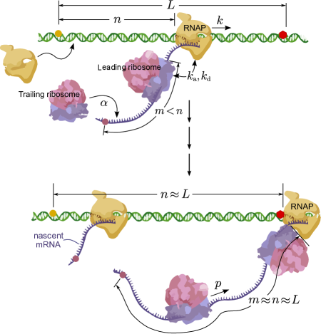
Figure 1: Schematic of translation of a nascent mRNA transcript (polypeptide not shown). Ribosomes translocate at rate $p$ while RNAPs elongate at rate $q$. Top: The transcript associated with the RNAP at position $n$ along the gene is shown with a leading ribosome at position $m$ along the mRNA. Ribosomes attach to open initiation sites at rate $\alpha$. Bottom: A nearly complete transcript is shown. If the leading ribosome has caught up to the RNAP and $m$ is close to $n$, the two may bind with rate $k_{\rm a}$ to form a “collided expressome.” Ribosome-RNAP complexes can spontaneously dissociate with rate $k_{\rm d}$. We assume the leading ribosome “terminates” upon reaching the stop codon (not shown). Protein-mediated expressomes (not shown) form larger complexes that can accommodate longer mRNA segments within it.

Both potential coupling mechanisms require at least some moments of close proximity between the RNAP and the leading ribosome during the simultaneous transcription-translation process (see Fig. 1), followed by recruitment of NusG for the NusG-coupled expressome mechanism. The ribosome-RNAP proximity requirement can be met if the ribosome elongation speed is, on average, faster than that of the RNAP. Even if the ribosome is fast, proximity also depends on initial condition (ribosome initiation delay after RNAP initiation) and the length of the transcript $L$. Moreover, both RNAPs and ribosomes are known to experience, respectively, pausing through backtracking (Zuo2022) and through “slow codons” for which the associated tRNA is scarce (Lakatos2004).

A number of open questions remain. In the “strong coupling” picture, the ribosome and RNAP are nearly always in contact and the speed of the ribosome is thought to limit that of the RNAP. Since under typical growth conditions, a ribosome translocates at the same 45nt/s speed as RNAP, the strong coupling picture provides an attractive explanation for the slowdown from 90nt/s in rRNA transcription to 45nt/s in mRNA transcription (Vogel1994). Administration of antibiotics to slow down translation also slowed down transcription.

However, other experiments have shown that the distance between the ribosome and RNAP can be large most of the time, leading to a “weak coupling” picture (Chen2018, Zhu2019). The biological role of weak coupling is unclear since any shielding provided by the ribosome would be limited and ribosome and RNAP speeds could be independently modulated. Even though direct ribosome-RNAP interactions may still arise after an RNAP has stalled for a sufficiently long time, any apparent ribosome-RNAP coordination would be largely coincidental.

Besides the strong and weak coupling dichotomy, another unknown is whether there are direct molecular interactions between the leading ribosome and RNAP. Although experiments to probe such interactions during normal transcription and translation in vivo will be difficult to design, our model can provide easier-to-measure indicators of molecular coupling.

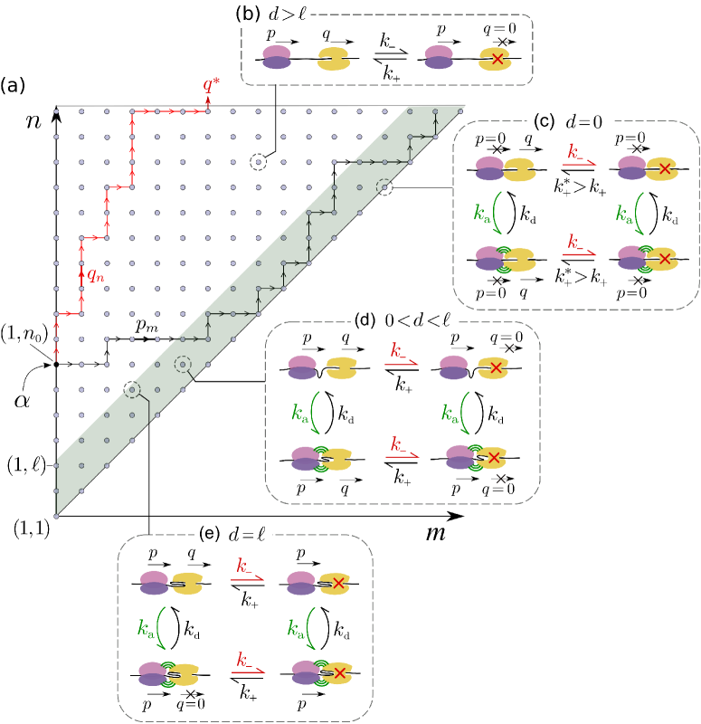
Figure 2: (A) State space of the stochastic model defined in terms of the leading ribosome and RNAP positions $(m,n)$. The initial time $t=0$ is defined as the time RNAP first produces a ribosome initiation site, starting the system in $(m=0,n=1)$. For $t>0$, as the RNAP is elongating, the first ribosome binds at rate $\alpha$. Here, a ribosome binds after the RNAP first reaches position $n=n_{0}$. Red and blue trajectories indicate scenarios in which the RNAP is relatively fast and slow, respectively. Within each position $(m,n)$ exist internal molecular microstates states. (B) In the “interior” states $n-m>\ell$ ($\ell=2$ in this example), the ribosome and RNAP are too distant to be bound, and only stalled and processing RNAP states arise, with transition rates $k_{\pm}$ between them. (C) When $n=m=0\leq\ell$, the ribosome and RNAP are adjacent without any intervening mRNA, allowing them to associate with rate $k_{\rm a}$. The RNAP can be in either stalled or processive states. In the stalled state, whether associated or not, the adjacent volume-excluding ribosome entropically “pushes” the stalled RNAP, catalyzing its transition to a processive state so that $k_{+}^{*}>k_{+}$. (D) When $0<n-m<\ell$, the ribosome and the RNAP are close enough to bind with rate $k_{\rm a}$. Here, the intervening mRNA dissipates the entropic pushing (so that the stalled RNAP $\to$ processing RNAP transition rate is $k_{+}$) and also allows an RNAP in the processive state to elongate with rate $q$, regardless of whether it is bound to the ribosome. (E) Only when the ribosome and the RNAP are separated by $d=\ell$ is a bound RNAP prevented from processing as this would reel in more mRNA than can be fit inside a collided expressome. Molecular binding prevents complexed ribosome and RNAP to be separated by more than $\ell$ mRNA codons.

To help resolve the puzzles discussed above, provide a quantitative way to explore different molecular mechanisms that may contribute to TTC, and generate predictions that can be compared to experimental observations, we formulate a stochastic model that combines a number of known molecular mechanisms from transcription, keeping track of ribosome and RNAP states and positions along the gene. While an earlier model combined transcription and translation in prokaryotes (Makela2011), it did not explicitly incorporate mechanisms of direct transcription and translation coupling and only assumed simple volume exclusion between the RNAP and the leading ribosome.

Here, we explicitly allow for RNAP pausing and direct association and dissociation of the ribosome-RNAP complex. The typical assay used to probe TTC involves measuring the time delay $\Delta T=T_{\rm rib}-T_{\rm RNAP}$ between the completion of mRNA and its associated protein. Although time delays can be used as a metric for defining transcription-translation coupling, absence of delay is a necessary but not sufficient condition for direct ribosome-RNAP coupling. A small mean delay time can arise simply from coincidental proximity of the ribosome to the RNAP at the time of termination. On the other hand, a significant time delay may indicate an uncoupled process especially if the delay is variable and cannot be controlled (Johnson2020). After formulating our model, we construct additional metrics that better define TTC. However, since the time delay is the most experimentally measurable quantity, we will still derive and compute the full probability density of delay times $\rho(\Delta T)$.

Model and Methods

Table 1: Model parameters

Params.	Description	Typical valuesa	Refs.
$\alpha$	translation initiation rate	$\sim 0.01-10.0$ $s^{-1}$	(Dai2016dec, Johnson2020, Shaham2017nov, Kennell1977jul) b
$L$	gene and transcript length	$L\in\mathds{Z}^{+},\,L\sim 300$	(Xu2006)
$m$	ribosome position from mRNA 5’	$m\in\mathds{Z}_{\geq 0},\,0\leq m\leq L$	–
$n$	RNAP position from mRNA 5’	$n\in\mathds{Z}_{+},\,m\leq n\leq L$	–
$p$	free ribosome translocation rate	$\sim 15$ codons/s	(Johnson2020, Young1976, Proshkin2010, Zhu2016)
$q$	free processing RNAP transcription rate	$\sim 30$ codons/s	(Proshkin2010, Iyer2018, Vogel1994, Epshtein2003may)c
$k_{-}$	processive RNAP $\to$ paused RNAP rate	$\sim 0.4$ $s^{-1}$	(Neuman2003) d
$k_{+}$	paused RNAP $\to$ processive RNAP rate	$\sim 0.3$ $s^{-1}$	(Neuman2003)
$k_{+}^{*}$	paused RNAP $\to$ processive RNAP rate (pushed)	$k_{+}^{*}=k_{+}\exp(E_{+}),E_{+}\geq 0$	estimated
$k_{\rm a},k_{\rm d}$	ribosome-RNAP association, dissociation rates	$k_{\rm d}=k_{\rm a}e^{-E_{\rm a}}$, $E_{\rm a}\sim 3-7$	(Fan2017)
$\ell$	maximum mRNA length in bound complex	$\sim 4-6$ codons	(Wang2020aug)e

• Ribosome and RNAP positions are measured in numbers of nucleotide triplets (codons) from the 5’ end of the nascent mRNA. For simplicity, we assume RNAP and ribosome initiation sites are coincident along the sequence.

• The translation initiation rate $\alpha$ depends on ribosome availability and varies significantly across the genome (Shaham2017nov, Siwiak2013sep). The median transcription initiation time is estimated to be $15-30$ seconds. For LacZ induction methods used in experiments, the initiation rates were assumed to be quite high. The definition of starting time depends on the experimental protocol and measurement. In (Johnson2020), the initiation time was neglected. In (Dai2016dec), the total time for initiation steps–including IPTG penetration, LacI depression, transcription initiation, and translation initiation–was measured to be around 10 seconds. Slow translation initiation can be compensated for by transcription arrest near the 5’ proximal region of the gene (Hatoum2008), allowing for a smaller $n_{0}$ (see Fig. 2). In our simulations, we set $\alpha=1$/s.

• Typical noninteracting RNAP transcription rates are $\bar{q}\sim 15$ codons/s. Since typically $k_{+}/(k_{+}+k_{-})\sim 1/2$, we use typical values $q\sim 30$ codons/s for the unimpeded transcription rate of processing RNAP.

• The pausing probability along an RNAP trajectory has been measured as $\sim 0.87$ per 100 nucleotides. By using the estimated mean RNAP velocity of $~{}\sim 15$ codons/s, we convert this probability to a pausing rate $k_{-}\approx 0.4$/s.

• The typical interaction range $\ell$ will be approximated by the maximum stored length of mRNA in a complex. For collided expressomes, $\ell\sim 4$ codons, while for NusG-mediated complexes, $\ell\sim 8$ codons since its larger size can accommodate more intervening mRNA.

Based on existing structural and interaction information, we formulate a continuous-time Markov chain to model ribosome and RNAP kinetics. As shown in Fig 1, we describe the position of the head of the leading ribosome along the nascent transcript by $m=0,1,\ldots,L$, where $0$ denotes a ribosome-free transcript. We also track the length of the nascent mRNA transcript that has cleared the exit channel of the RNAP through the discrete variable $n=1,2,\ldots,L$. The positions are described in terms of triplets of nucleotides corresponding to codons, the fundamental step size during ribosome elongation. Here, $L$ is the length of the gene, typically about $L\sim 300$ codons. We carefully choose the definition of $m$ and $n$ so that ribosome and RNAP sizes are irrelevant and that the difference $d\equiv n-m$ precisely describes the length of the free intervening mRNA between them. While this assumption is certainly not true due to shorter leading and termination segments specific to translation, the slight differences in length are assumed negligible, or are subsumed in effective translation initiation rates. Therefore, $0\leq m\leq L$ and $1\leq n\leq L$, where $n=L$ is interpreted as a completion mRNA and $m=L$ is interpreted as a completed polypeptide. This triangular state-space structure has arisen in related stochastic models of interacting coordinates in one-dimension (Chou2007, Zuo2022, Kolomeisky2022).

Here, within each positional state $(m,n)$, the leading ribosome and RNAP can exist in different internal configurations describing their molecular states. The RNAP at site $n$ can switch between two states, a processive state and a paused state. In the processive state, the RNAP can move forward by one codon at rate $q_{n}$ or it can transition to a paused or “backtracking” state with stalling rate $k_{-}$. The RNAP elongation rate can also depend on its position $n$ through different abundances of corresponding nucleotides. For simplicity, we assume that RNAPs in the backtracking state are fixed and do not elongate ($q_{n}=0$) but may transition back to the processive state with “unstalling” rate $k_{+}$. The waiting time distributions in the processive and paused states are exponential with mean $1/k_{-}$ and $1/k_{+}$, respectively. The leading ribosome at site $m$ will be assumed to always be in a processive state with forward hopping rate $p_{m}$ if and only if the next site $m+1$ is empty (not occupied by the downstream RNAP). In general, the ribosome translation rate can depend on the position $m$ through the codon usage at that site.

When the distance between the leading ribosome and the RNAP is within an interaction range $\ell$, ($d\equiv n-m\leq\ell$), they may bind with rate $k_{\rm a}$ to form a collided expressome and dissociate with rate $k_{\rm d}$ (Eq. 6 and 7). To enumerate internal states that are associated/disassociated and processing/backtracking, we define $(a,b)\in\left\{0,1\right\}^{2}$ such that $a=1$ refers to an associated, or “bound” ribosome-RNAP complex, and $b=1$ refers to an RNAP in a backtracking, or a “paused” or “stalled” state. When $a=0$, the ribosome is not bound to the RNAP, and when $b=0$, the RNAP is in the processive state. The state space of our discrete stochastic model is given by $\left\{(m,n,a,b):1\leq m\leq n\leq L,a\in\{0,1\},b\in\{0,1\}\right\}$, with  
$\left\{(0,n,0,b):1\leq n\leq L,b=\pm 1\right\}$ representing ribosome-free configurations.

Other than steric exclusion (which constrains $m\leq n$) and ribosome-RNAP association and dissociation, we incorporate a contact-based RNAP “pushing” mechanism. The processing ribosome can directly push (powerstroke) against a stalled RNAP and/or reduce the entropy of a backtracking RNAP to bias it towards a processive state. A similar mechanism arises in RNAP-RNAP interactions as discussed in (Zuo2022). To quantify this pushing mechanism, we simply modify the paused-to-processive RNAP ($b=1\to b=0$) transition rate from $k_{+}$ to $k_{+}^{*}\equiv k_{+}e^{E_{+}}>k_{+}$ whenever the ribosome abuts the RNAP ($d\equiv n-m=0$). The enhanced rate arises from a reduction $E_{+}$ in the total transition free energy barrier provided by the adjacent ribosome. Typical model parameters relevant to prokaryotic transcription and translation are listed in Table 1.

The length $\ell$ may influence direct molecular coupling and stochastic dynamics of transcription. In vitro studies of ribosome and RNAP structure provide constraints on the configuration space accessible to coupled expressomes. Wang et al. (Wang2020aug) found that collided expressomes are stable only when the spacer mRNA between the ribosome and the RNAP is $\sim~{}12-24$ nucleotides ($\sim 4-8$ codons). Because the intervening mRNA must be at least $12$ nucleotides to extend beyond the RNA exit channel of the RNA polymerase, the free intervening RNA within an intact collided expressome can vary between 0 and 12 nucleotides. In contrast, the NusG-mediated expressome can accommodate $\sim 24-30$ free mRNA nucleotides. RNA looping might allow for even longer spacer mRNA, but there has so far been no in vivo evidence that collided expressomes exist with mRNA loops.

Since mRNA is flexible, we can also assume that $k_{\rm d}$ is constant for $d\equiv n-m\leq\ell$. The association rate $k_{\rm a}$ may be dependent on the distance $d=n-m$ between the ribosome and the RNAP; for example, a distance-dependent association rate might take the form $k_{\rm a}(n-m)\approx k_{\rm a}(\ell)[(\ell+\xi)/(n-m+\xi)]^{3}$, where $[(n-m)+\xi]^{-3}$ represents the effective volume fraction of the leading ribosome and $\xi$ is the configuration flexibility of ribosome-RNAP binding when they are close. If we adopt such a distance-dependent $k_{\rm a}$, we would also have to let the ratio $p/q$ be dependent on $(n-m)$ in order conserve free energy during approach and binding steps. To simplify matters, we will assume $\xi\gg\ell$ and take $k_{\rm a}$ to be a constant for $d\equiv n-m\leq\ell$ and zero for $d\equiv n-m>\ell$.

The overall kinetics of the internal states pictured in the insets of Fig. 2 can be explicitly summarized by considering the intervening mRNA length $d=n-m$ between RNAP and the ribosome.

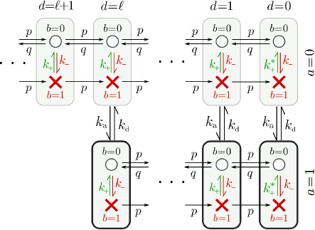
Figure 3: Internal state space associated with different values of the ribosome-RNAP distance $d=n-m$. Open circles ($b=0$) represent states with processing RNAP that allow $d$ to increase and decrease with rate $q$ and $p$, respectively. Processing states can transition with rate $k_{-}$ to states that contain a paused RNAP (red crosses, $b=1$, $q=0$). When $0\leq d\leq\ell$, transitions between coupled and uncoupled states occur at rate $k_{\rm d},k_{\rm a}$. When $d=\ell$ and $a=1$, the coupled RNAP cannot proceed, even if it is processive, without first dissociating from the ribosome. Only after detachment ($a=0$) can the separation exceed $\ell$, during which binding cannot occur and the ribosome and the RNAP process independently without the tethering constraint. Thus, bound states with $a=1$ (and $0\leq d\leq\ell$) describe a kinetic trap in which the ribosome and RNAP are tethered by the $\ell$-length mRNA and overall transcription can occur only through inchworming. Whether bound or unbound, when $d=0$, the ribosome increases the RNAP unstalling rate from $k_{+}$ to $k_{+}^{*}=k_{+}e^{E_{+}}$.

Fig. 3 explicitly depicts the transitions as a function of $d$. Since in our model, the maximum length of mRNA that can fit within the complex is $\ell$, a processing ribosome-bound RNAP at $n=m+\ell$ cannot advance to lengthen the already compressed transcript. The only way a coupled state $a=1$ with $d=\ell$ can reach any state where $d>\ell$ is for the ribosome and RNAP to first dissociate (we assume dissociation rates in all $d=n-m$ states remain constant at $k_{\rm d}$). Molecular coupling effectively slows down transcription by preventing RNAP elongation in the $a=1,d=\ell$ state. Such ribosome-mediated slowing down of transcription has been proposed in previous studies (Stevenson-Jones2020, Kohler2017apr).

We now list all allowed transitions in the $\omega\coloneqq\{m,n,a,b\}$ state space of our continuous-time stochastic Markov model. The probability that an allowable transition from state $s$ to state $s^{\prime}$ occurs in time increment $\textrm{d}t$ is $r(\omega^{\prime}|\omega)\textrm{d}t$ where the complete set of rates is given by

$$r(1,n,a,b\,|\,0,n,a,b) =\alpha, 1\leq n\leq L,$$ (2)

$$r(m+1,n,a,b\,|\,m,n,a,b) =p_{m}, 1\leq m\leq n-1,$$ (3)

$$r(m,n+1,0,0\,|\,m,n,0,0) =q_{n}, m\leq n\leq L-1,$$ (4)

$$r(m,n+1,1,0\,|\,m,n,1,0) =q_{n}, 0\leq d\leq\ell-1,$$ (5)

$$r(m,n,1,b\,|\,m,n,0,b) =k_{\textrm{a}}, 0\leq d\leq\ell,$$ (6)

$$r(m,n,0,b\,|\,m,n,1,b) =k_{\textrm{d}},$$ (7)

$$r(m,n,a,1\,|\,m,n,a,0) =k_{-},$$ (8)

$$r(m,n,0,0\,|\,m,n,0,1) =k_{+},$$ (9)

$$r(m,n,1,0\,|\,m,n,1,1) =k_{+}^{*}, a=1,m=n.$$ (10)

Using these rules, we performed event-based stochastic simulations (Bortz1975, Gillespie1977dec) of the model as detailed in Appendix S1 of the Supplemental Information (SI). For completeness, the master equation associated with our model is also formally given in Appendix S2.

Construction of time delay distribution.

Our model allows for explicit calculation of the distribution $\rho(\Delta T)$ of time delay $\Delta T$. To find $\rho(\Delta T)$, we first find the distribution of ribosome positions $m(T_{i})$ at the moment $T_{i}\equiv T(n=i)$ the RNAP first reaches site $i$. $T_{L}\equiv T_{\rm RNAP}$ denotes the instant the mRNA is completed. The initial value $m(T_{1})=0$ is known because immediately after initiation of RNAP at site $n=1$, the ribosome is not yet present but is trying to bind at a rate of $\alpha$. As detailed in Appendix S3, we can iteratively find the distribution of $m(T_{i+1})$ given that of $m(T_{i})$. By the same method, the distribution of association values $a(T_{\rm RNAP})$ at the instant of RNAP completion can be computed. After constructing the probability distribution $\mathbb{P}(m,a,b\,|\,t=T_{\rm RNAP})$, we can construct the probability density $\rho(\Delta T)$ of the mRNA protein time delay $\Delta T\equiv T_{\rm rib}-T_{\rm RNAP}$ by evaluating the distribution of times required for the ribosome to catch up by reaching $m=L$.

Although we are able to construct the whole distribution of delay times that might provide a more resolved metric, especially if single-molecule assays can be developed, a short time delay is a necessary but not sufficient condition for TTC. To provide direct information on molecular ribosome-RNAP interactions, we construct additional metrics.

Coupling indices.

To more explicitly quantify direct molecular coupling, we also define the coupling coefficient $C$ by

$$C\equiv\mathbb{P}(a\,|\,t=T_{\rm RNAP}),$$ (11)

the probability that the ribosome is associated with the RNAP ($a=1$) at the moment the mRNA transcript is completed. The coupling parameter $C$ provides a more direct measure of molecular coupling and further resolves configurations that have short or negligible delays. While delay time distributions do not directly quantify ribosome-RNAP contact, the coupling coefficient $C$ does not directly probe the trajectories or history of ribosome-RNAP dynamics.

To also characterize the history of ribosome-RNAP interactions, we quantify TTC by the fraction of time $F_{T}$ that the ribosome “protects” the RNAP across the entire transcription process. There are different ways of defining how the transcript is protected. While both modes of TTC are proposed to shield the mRNA from premature termination, neither has been directly observed in vivo. We assume that a termination protein has size $\sim\ell_{\rm p}$ and that if the ribosome and RNAP are closer than $\ell_{\rm p}$, the termination factor is excluded. Thus, we define the protected time as the total time that $d<\ell_{\rm p}$ codons, divided by the time to complete transcription:

$$F_{T} =\frac{\left\lVert\left\{t:(n_{t}-m_{t}<\ell_{\rm p})\right\}\right\rVert}{T_{\rm RNAP}}.$$ (12)

Since the transcription-termination protein Rho has an mRNA footprint of about $80$nt, $\ell_{\rm p}\approx 27$ codons (Koslover2012nov). The protected-time fraction $F_{T}$ provides yet another metric for TTC that measures the likelihood of completion.

Using these metrics and the effective velocities $\overline{V}_{\rm rib}$ and $\overline{V}_{\rm RNAP}$, we will explore the biophysical consequences of our model. Simple limits are immediately apparent. If the free ribosome translocation rate is much greater than the free RNAP transcription rate and $\alpha\gg L/\bar{q}$, the ribosome, for much of the time, abuts against the RNAP, inducing it to transcribe at rate $qk_{+}^{*}/(k_{+}^{*}+k_{-})\equiv\bar{q}^{*}$. Here, we predict an expected delay $\Delta\overline{T}\approx 0$, $C\approx k_{\rm a}/(k_{\rm a}+k_{\rm d})$, and $F_{T}\approx 1$. If the ribosome is slow and $p\ll\bar{q}$, the ribosome and RNAP are nearly always free, $\Delta\overline{T}\approx 1/\alpha+L(1/p-1/\bar{q})$, $C\approx 0$, and $F_{T}\approx 0$. However, when $p$ is intermediate, more intricate behavior can arise, including tethered elongation and transcription slowdown. In the next section, we focus on the intermediate translation rate regime and show how the effective velocities defined in Eq. 1 and $F_{T}$ characterize the functional dynamics of TTC and $C$ characterizes the intrinsic properties of TTC, even though $\rho(\Delta T)$ remains the most easily measurable property of TTC.

Results and Discussion

Here, we present analyses of solutions to our model obtained from numerical recursion and Gillespie-type kinetic Monte Carlo simulations detailed in Appendices S1, S2, and S3 of the SI. Predictions derived from using different parameter sets are compared, and mechanistic interpretations are provided.

Comparison of coupling indices

We evaluate our stochastic model to provide quantitative predictions for the coupling indices, $\rho(\Delta T)$, $C$, $\mathbb{E}[F_{T}]$. The results are summarized in Fig. 4.

Limitations of mean delay time.

Fig. 4(A) shows delay-time distributions for various parameter sets and reveals subtle differences in the kinetic consequences of coupling. Without molecular coupling $(k_{\rm a}=0)$, the distribution has a single peak around the mean delay time. With molecular coupling, the distribution can exhibit two peaks with one at $\Delta T=0$. This short-time peak reflects trajectories that terminate as a bound ribosome-RNAP complex. These finer structures in $\rho(\Delta T)$ cannot be resolved by evaluating only the mean delay time. Fig. 4B plots the mean delay $\Delta\overline{T}$ as a function of $p$ and $q$. For our chosen parameters, in particular $k_{\rm a}=100$ s^-1 and $k_{\rm d}=k_{\rm a}e^{-3}$, we see that $\Delta\overline{T}$ is rather featureless, with a significant delay arising only for small $p$. Thus, the mean delay time provides little information about the details of TTC.

Coupling coefficient.

From an effective velocity argument (see Appendix S4 in the SI), we approximate the criterion for coupling in terms of

$$\frac{p}{\bar{q}}\equiv\frac{p}{q}\frac{k_{-}+k_{+}}{k_{+}},$$ (13)

where $\bar{q}$ is the average pausing-adjusted RNAP transcription rate $\bar{q}\equiv qk_{+}/(k_{+}+k_{-})$. This dimensionless ratio $p/\bar{q}$ is a key indicator of the overall level of coupling possible. If $p/\bar{q}>1$, the speed of the ribosome exceeds the average speed of the RNAP, allowing them to approach each other and potentially form a collided expressome. If $p/\bar{q}<1$, the ribosome speed is slower than the average RNAP speed and the system can at most be only transiently coupled. It turns out that the coupling coefficient $C$ is mostly determined by $p/\bar{q}$ alone, particularly if all other parameters are kept fixed. Essentially, the transition to a coupled system (large $C$) is predicted when $p/\bar{q}\gtrsim 1$. In Fig. 4C, we find the values of $C$ for multiple values of $p$ and $q$ [each dot corresponds to each $(p,q)$ pair], and plot them as a function of $p/\bar{q}$, with $k_{+}/(k_{+}+k_{-})\approx 0.43$. The mean values of $C$ as a function of $p$ and $q$ are plotted in Fig. 4D and are qualitatively distinct from the mean times shown in (B).

Fraction of time protected.

Each point in Fig. 4E indicates the mean value $F_{T}$, $\mathbb{E}[F_{T}]$, for different values of $p$ and $q$, arranged along values of $p/\bar{q}$. Each mean value $\mathbb{E}[F_{T}(p,q)]$ was computed from averaging protected-time fractions $F_{T}$ (Eq. 12) from 1000 simulated trajectories. As expected, $\mathbb{E}[F_{T}(p,q)]$ increases linearly with ribosome translation rate $p$ until saturation to above $\mathbb{E}[F_{T}]\gtrsim 0.9$ for $p\gtrsim 22$ codons/s.

Comparing $C$ and $\mathbb{E}[F_{T}]$ from Figs. 4D and F, we find that $C$ and $\mathbb{E}[F_{T}]$ are qualitatively similar across various values of $p$ and $q$, although in general we find $\mathbb{E}[F_{T}]\gtrsim C$. The transition from low to high values occurs at lower values of $p$ for $\mathbb{E}[F_{T}]$ since the condition for protection ($d\leq\ell_{\rm p}$) is not as stringent as that for $C=1$ ($d\leq\ell$ and binding). Thus, there can be value of $(p,q)$ for which $C(p,q)$ is small but $\mathbb{E}[F_{T}(p,q)]$ is close to one.

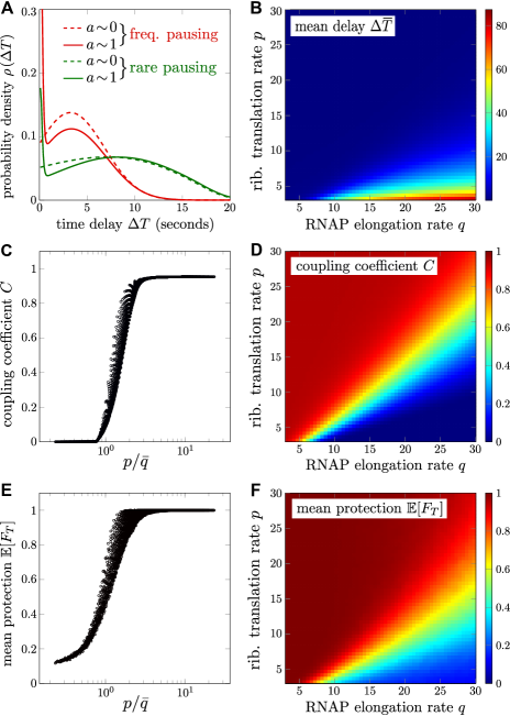
Figure 4: Comparison of different TTC indices. Common parameters for all these plots are $\alpha=1$/s, $E_{+}=2$, $E_{\rm a}=3$, $k_{\rm d}=k_{\rm a}e^{-E_{\rm a}}$, $\ell=4$, $L=335$, and $k_{\rm a}=100$/s unless stated otherwise. (A) The delay-time distribution $\rho(\Delta T)$ calculated under different parameter regimes using Algorithm 1 (see SI). Here, $p=12$ codons/s, $q=30$ codons/s, $k_{+}=0.4$/s, $k_{-}=0.3$/s for rarely pausing RNAPs (red curves), and $k_{+}=4.0$/s, $k_{-}=3.0$/s for frequently pausing RNAPs (blue curves). Fast-binding ($a\sim 1$, $k_{\rm a}=100$/s, $k_{\rm d}=k_{\rm a}e^{-3}$) and no-binding ($a=0$, $k_{\rm a}=0$) cases are indicated by solid and dashed curves, respectively. (B) Mean delay $\Delta\overline{T}$ as a function of $p$ and $q$. (C) The direct coupling coefficient $C$ as a function of the relative velocity $p/\bar{q}$. Each point represents $C$ evaluated at specific values of $(p,q)$, each chosen from all integers between $3$ and $27$ codons/s. (D) Heatmap of $C(p,q)$. (E) Values of $\mathbb{E}[F_{T}]$, each derived from 1000 kinetic Monte-Carlo (kMC) trajectories, plotted against $p/\bar{q}$. (F) The heatmap of $\mathbb{E}[F_{T}(p,q)]$.

The similarity between $\mathbb{E}[F_{T}]$ and $C$ is restricted to the dependence on $p$ and $q$. The coupling and the protection time fraction may respond to changes in other parameters in drastically different ways. For example, $C$ is nonzero only if molecular binding is present, rendering it sensitive to $k_{\rm a},k_{\rm d}$. However, $F_{T}$ directly measures the dynamics of TTC and does not depend on actual molecular coupling, so it will be relatively insensitive to $k_{\rm a},k_{\rm d}$, particularly when $p$ is large. Thus, $F_{T}$ may be a better index if we wish to quantify functional consequences of TTC. The standard deviations of the simulated $F_{T}$ values are typically large and approximately $\sqrt{\mathbb{E}[F_{T}]\big{(}1-\mathbb{E}[F_{T}]\big{)}}$ (shown in Appendix variations of the SI), limiting the suitability of the mean protected-time fraction as a robust metric.

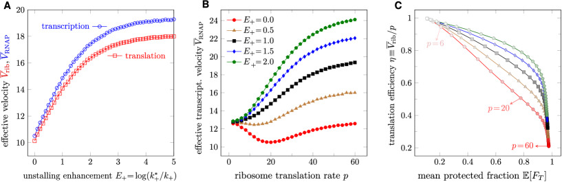
Figure 5: Slowdown induced by molecular coupling. The common parameters used are the same as those in Fig. 4. (A) Effective velocities as a function activation energy reduction $E_{+}=\log(k_{+}^{*}/k_{+})$ in ribosome-induced RNAP unstalling, $p=20$ codons/s and $q=30$ codons/s. (B) Effective velocity of RNAP as a function of the free ribosome translation rate $p$. (C) The trade-off between translation efficiency and mean fraction of time protected $\mathbb{E}[F_{T}]$. The efficiency $\eta\equiv\overline{V}_{\rm rib}/p$ is defined by the ratio of the mean ribosome speed to the translation rate of an isolated ribosome. In (B) and (C), $q=30$ codons/s. The variances (not shown) for the plotted quantities are large, typically overlapping the mean-value curves in (A) and (B).

Binding-induced slowdown

Traditionally, TTC has been invoked as a mechanism for maintaining RNAP processivity by rescuing RNAP from paused states. However, in vivo experiments by Kohler et al. (Kohler2017apr) reported that when translation is inhibited, the $\Delta\alpha\textrm{CTD}$ mutant in which RNAP does not associate with ribosome exhibited faster proliferation than that of wild-type RNAP that can associate with ribosomes. Coupled transcription through ribosome-RNAP association may give rise to slower transcription. Thus, TTC may play dual roles of speeding up and slowing down transcription, depending on conditions. Through our model, we will explain the major mechanism of, and limits to, TTC-induced slowdown of transcription.

Unstalling rate $k_{+}^{*}$ dictates ribosome efficiency.

The principal factor that influences the overall velocity $\overline{V}$ of a coupled expressome is the interplay between two antagonistic mechanisms: ribosome-mediated dislodging of an adjacent stalled RNAP and bound-ribosome deceleration of the RNAP. When the reduction in activation free energy of unstalling, $E_{+}=\log(k_{+}^{*}/k_{+})$, is large, the ribosome is less likely to be impeded by a stalled RNAP. Fig. 5A plots the effective velocities $\overline{V}_{\rm rib}$ and $\overline{V}_{\rm RNAP}$ as a function of $E_{+}$ and illustrates the increases in overall speed when the ribosome is more effective at dislodging a stalled RNAP (higher $E_{+}$).

The decrease in the velocity of a coupled processing RNAP is primarily determined by the ribosome translation speed $p$. For different values of $E_{+}=\log(k_{+}^{*}/k_{+})$, the dependence of $\overline{V}_{\rm RNAP}$ on $p$ can be quite different, as is shown in Fig 5B. For large $E_{+}$, when the ribosome efficiently pushes stalled RNAPs, increasing $p$ allows the ribosome to more frequently abut the RNAP and dislodge it, leading to faster overall transcription. However, for inefficient unstalling (small $E_{+}$), we see that faster ribosomes can decrease $\overline{V}_{\rm RNAP}$. This feature arises because for inefficient unstalling, a larger $p$ increases the fraction of time the ribosome and RNAP are bound $(a=1)$, allowing a binding-induced slowdown to arise more often. Besides $E_{+}$, the emergence of a decreasing transcription velocity $\overline{V}_{\rm RNAP}$ with increasing ribosome translation rate $p$ depends intricately on factors such as $\ell$, $k_{\pm}$, $k_{\rm a},k_{\rm d}$ and arises only if $k_{\rm a}/k_{\rm d}$ is sufficiently large and $\ell$ is not too large.

Although the decrease in $\overline{V}_{\rm RNAP}$ is not large, it certainly suggests that increasing $p$ under small $E_{+}\leq 0.5$ is not advantageous. This observation motivates us to define a translation efficiency as the ratio of the effective ribosome speed $\overline{V}_{\rm rib}$ to its unimpeded translation speed $p$: ${\eta}\equiv\overline{V}_{\rm rib}/p$. The loss $1-\eta$ measures how much a ribosome is impeded due to its interactions with the RNAP. As $p$ is increased, we find trajectories that display a trade-off between translation efficiency and protected time. Higher $p$ leads to more proximal ribosomes and protected RNAP at the expense of translation efficiency $\eta$. Fig. 5C shows that the decrease in unstalling activation energy $E_{+}$ affects this level of trade-off. For large $E_{+}$, increasing $p$ can speed up ribosomes beyond the velocity determined by $\bar{q}$ so that $\eta$ decreases more slowly than $\sim 1/p$. At the same time, the system is only slightly less coupled, leading to a subtle decrease in $\mathbb{E}[F_{T}]$. In the end, larger $E_{+}$ leads to a higher $\eta$ versus $\mathbb{E}[F_{T}]$ curve.

Low $\eta$s are likely selected against since a cell would be expending more resources than necessary to maintain high levels of tRNA and other translation factors. An potentially optimal setting may be to maintain $p\simeq\bar{q}$, which is the minimally sufficient velocity to keep the RNAP protected. This intermediate choice of $p$ for the ribosome may explain the recent observations that slower ribosomes did not appreciably slow down transcription (Zhu2019) or prevent folding of specific mRNA segments (Chen2018).

Limits of binding-induced slowdown.

In cases where $\bar{q}<p<q$ and $L\rightarrow\infty$, the mean velocity conditioned on coupling ($a=1$) can be estimated in the strong binding ($k_{\rm a}/k_{\rm d}\gg 1$), steady-state limit (see Eq. S25 in Appendix S4 of the SI):

$$\overline{V}_{\rm RNAP}\approx q\left[\frac{(q/p)^{\ell}-1}{(q/p)^{\ell+1}-1}\right]\frac{k_{+}^{*}}{k_{+}^{*}+k_{-}}.$$ (14)

For large $\ell\geq 1$ and sufficiently large $q/p$, the term $\left[\frac{(q/p)^{\ell}-1}{(q/p)^{\ell+1}-1}\right]$ is approximately $p/q$, and lower bounds for $\overline{V}_{\rm RNAP}(a=1)$ are

$$\overline{V}_{\rm RNAP}\geq\frac{pk_{+}}{k_{+}+k_{-}}\geq q\left(\frac{k_{+}}{k_{+}+k_{-}}\right)^{2}.$$ (15)

The first equality holds when $k_{+}^{*}=k_{+}$, and the second equality holds when $p=\bar{q}$. We conclude that the maximum slowdown induced by binding is essentially limited by the slowdown of RNAP due to transcriptional road blocks. The latter plays a fundamental role in the significantly slower rate of mRNA transcription relative to rRNA transcription.

Testing the molecular coupling hypothesis

Since there has not been direct observation of molecular coupling in vivo, it is informative to compare scenarios that predict molecular coupling to those that do not. We now vary the binding energy $E_{\rm a}$ for different velocity ratios $p/\bar{q}$. For $\ell=4$, Fig. 6A shows $\overline{V}_{\rm RNAP}$ as a function of $E_{\rm a}$ for various values of $p$. Although higher $p$ leads to increased $\overline{V}_{\rm RNAP}$, for each value of $p$, increasing the binding energy increases coupling and leads to RNAP slowdown. Both $p$ and $E_{\rm a}$ increase $\mathbb{E}[F_{T}]$ as shown in Fig. 6B. As different values of $E_{\rm a}$ are used, we also find a trade-off between ribosome efficiency and protection, as shown in Fig. 6C. In Appendix S6, we provide additional simulation results that confirm the $\ell$-dependence in Eq. 14 and in $\mathbb{E}[F_{T}]$.

Our predicted differences in effective velocities $\overline{V}$ and $\mathbb{E}[F_{T}]$ are probably not significant enough to be easily distinguished experimentally; thus, we investigate the distribution of delay times $\rho(\Delta T)$ as $p$ is varied. Fig. 6D shows $\rho(\Delta T)$ rescaled so that the largest value is set to unity for easier visualization. We see that for intermediate values of $10\lesssim p\lesssim 13$, $\rho(\Delta T)$ can be bimodal. Fig. 6E depicts a single-peaked $\rho(\Delta T)$ when coupling is completely turned off by setting $k_{\rm a}=0,(E_{\rm a}=-\infty)$. In this case, $\ell$ is irrelevant. Fig. 6F shows the rescaled $\rho(\Delta T)$ in the presence of coupling ($E_{\rm a}=3$) for $\ell=40$. Here, there are two regimes, $8\lesssim p\approx 12$ and $18\lesssim p\lesssim 24$, that exhibit bimodality.

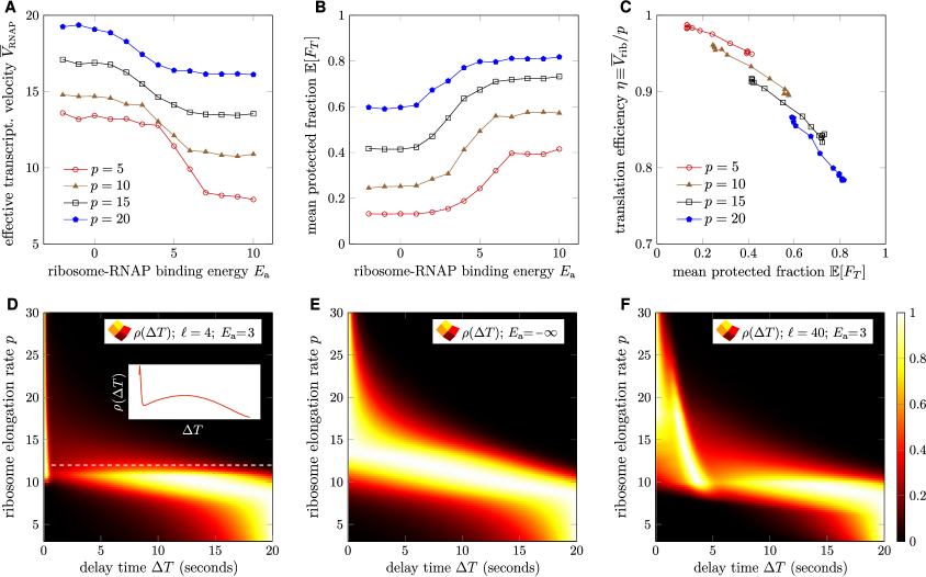
Figure 6: Effects of molecular coupling. For those parameters not varied, we use the same values used to generate Figs. 4 and 5. (A) For $\ell=4$, the effective transcription velocity $\overline{V}_{\rm RNAP}$ as a function of binding-energy depth between the ribosome and RNAP $E_{\rm a}$. (B) Mean protected-time fraction $\mathbb{E}[F_{T}]$ as a function of binding energy depth $E_{\rm a}$ ($\ell=4$). (C) The trade-off between efficiency and protection for $\ell=4$. (D) Rescaled heatmap of the delay-time distribution $\rho(\Delta T)$ as a function of ribosome translocation rate $p$. The brightness indicates the relative probability, and the inset shows the probability distribution at $p=12$ codons/s indicated by the dashed white line. Here, the binding energy $E_{\rm a}=3$ and $\ell=4$. For $p\approx 9$ codons/s, $\rho(\Delta T)$ is bimodal in $\Delta T$. (E) Delay-time distribution in the absence of ribosome-RNAP binding ($k_{\rm a}=0$). Here, the $\ell$-dependence disappears and $\rho(\Delta T)$ is monomodal. (F) Delay-time distribution for $\ell=40$ and $E_{\rm a}=3$. Bimodality arises in more than one regime of $p$.

Genome-wide variability of coupling

We have so far assumed all parameters are homogeneous along the transcript and time-independent. However, a cell is able to dynamically regulate the transcription and translation of different genes by exploiting the transcript sequence or other factors that mediate the process. Such regulation can be effectively described within our model by varying its parameters in the appropriate way.

Regulation of RNAP pausing.

The RNAP pausing rate $k_{-}$ is one parameter that can be modulated by specific DNA sequences and other roadblocks along the gene (Komissarova1997, Epshtein2003may, Nudler2009, John2000). There is evidence that consensus pause sequences are enriched at the beginning of genes (Hatoum2008, Larson2014may). In addition to leading ribosomes, a trailing RNAP can also push the leading RNAP out of a paused state by increasing $k_{+}$, much like ribosomes (Epshtein2003may, Zuo2022). Even if $k_{+}$ and $k_{-}$ are varied in our model, the overall predicted performance regimes of the system are still delineated by values of $p/\bar{q}$, and the effective transcription velocity can still be predicted by Eq. 14.

Effects of translation initiation rates.

Translation initiation is another process that can be altered by the cell through, e.g., initiation factors that modulate the initiation rate $\alpha$ (Chou2003). Genome-wide analysis reveals that translation initiation times in E. coli are highly variable, ranging from less than 1 second to more than 500 seconds (Siwiak2013sep, Shaham2017nov).

As shown in Figs. 7A-C, varying the translation initiation rate $\alpha$ straightforwardly affects TTC. As indicated in (A), the predicted $\overline{V}_{\rm RNAP}$ at $\alpha\simeq 1\textrm{s}^{-1}$ is preserved across different values of $p$. Slower translation initiation results in larger initial separations $n_{0}$, decreasing the overall fraction of protected times, as shown in (B) and (C). To mitigate large initial distances $n_{0}$ and lower likelihood coupling due to slow initiation, RNAP pausing occurs more often at the start of the gene to allow time for a slow-initiating ribosome to catch up. Thus, delayed ribosome initiation and early RNAP pausing are two “opposing” processes that can regulate coupling and efficiency, especially for short genes.

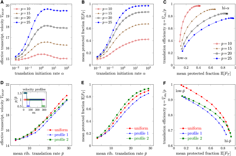
Figure 7: TTC and performance under genomic variability. Again, we use the standard set of fixed parameter values as in Figs. 5 and 6. (A) Effective transcription velocity $\overline{V}_{\rm RNAP}$ as a function of the translation-initiation rate $\alpha$. $\overline{V}_{\rm RNAP}$ initially increases as $\alpha$ is increased until about $\alpha\simeq 1$ s ^-1, after which $\overline{V}_{\rm RNAP}$ decreases slightly as $\alpha$ is further increased. (B) Mean protected fraction $\mathbb{E}[F_{T}]$ as a function of the translation-initiation rate $\alpha$. (C) Efficiency versus protection fraction as $\alpha$ is varied. Larger $\alpha$ contributes to both efficiency and protection. As $\alpha$ is increased, the system spends more time protected. Since $\overline{T}_{\rm rib}$ includes the ribosome initiation time, it decreases as $\alpha$ is increased, leading to an increased $\overline{V}_{\rm rib}$ and $\eta$. (D) and (E) $\overline{V}_{\rm RNAP}$ and $\mathbb{E}[F_{T}]$ as a function of the mean $\bar{p}$ under three different translocation rate profiles $p_{m}$. (F) The $\eta$-$\mathbb{E}[F_{T}]$ trade-off plot for three different profiles as the mean value $\bar{p}$ is varied. The inset in (D) illustrates the three translation-rate profiles. The overall performance of profile 1 suffers because of the slowdown following the initial fast translation. For $\bar{p}\leq 15$ codons/s, profile 2 has a higher $\overline{V}_{\rm RNAP}$ compared with the uniform profile. When $p\geq 15$ codons/s, the uniform profile still has a higher $\overline{V}_{\rm RNAP}$. For all values of $p$, profile 2 has a higher $F_{T}$ than the uniform profile because of its higher initial speed.

Ribosome translocation-rate profiles.

Although we have thus far assumed uniform ribosome translocation rates, it is known that codon bias and tRNA/amino acid availability can locally affect ribosome translocation (Lakatos2004, Klumpp2012). Snapshots of ribosome positions along transcripts have been inferred from ribosome profiling experiments. After imposing a stochastic exclusion model (MacDonald1969), Khanh et al. (DaoDuc2018jan) reconstructed position-dependent ribosome translocation rates $p_{m}$. They found that hopping rates $p_{m}$ are larger near the 5’ end and decreases towards the 3’ end. Although they reconstructed the entire genome-wide $p_{m}$ profile, translocation rates are gene-dependent, so we will propose and test simple profiles $p_{m}$.

To qualitatively match the inferred profile (DaoDuc2018jan), we define profile 1 by increasing $p$ by 50% for the first 40 codons, and decreasing it by 50% for the second 40 codons. The rest of the transcript retains the constant baseline value of $p$. Profile 2 is similarly defined except that instead of being the second group of 40 codons, the speed across the last 40 codons is decreased. We compared the performance of the three different profiles in Fig. 7D-F as a function of the mean translation rate $\bar{p}\equiv L^{-1}\sum_{m=1}^{L}p_{m}$. In the low-speed regime $\bar{p}\lesssim 10$ codons/s, higher starting $p_{m}$ values promote ribosome-RNAP interactions, leading to a slightly higher effective transcription velocity $\overline{V}_{\rm RNAP}$ and higher mean protected fraction $\mathbb{E}[F_{T}]$. However, in profile 1, the subsequent decrease in $p_{m}$ under strong coupling is sufficient to induce slowdown of RNAP. This nonmonotonic effect is weaker in profile 2 because by the later time that translational slowdown occurs, the machines are further apart (and less likely to be bound) since they are further removed from the common initial high-$p$ region. Fig. 7F shows that profile 2 provides the best protection, but increasing the likelihood of coupling means that profiles 1 and 2 are more likely to be impeded by stalled RNAP, leading to slightly lower ribosome efficiency $\eta$.

Summary and Conclusions

We have presented a detailed stochastic model of translation-transcription coupling (TTC). The continuous-time discrete-state model tracks the distance between the leading ribosome and the RNAP and assumes they sterically exclude each other along the nascent mRNA transcript. All current experimental understanding of interactions between RNAP and ribosome, including ribosome initiation, RNAP pausing, and direct ribosome-RNAP association have also been incorporated. Our model exhibits a number of rich features that depend on the interplay of these intermediate mechanisms.

To quantitatively investigate the predictions of our model, we constructed three different metrics to quantify TTC, the delay-time probability distribution $\rho(\Delta T)$, the probability $C$ that the ribosome and the RNAP are in a bound state $(a=1)$ at termination, and the fraction of time $F_{T}$ that the ribosome and the RNAP are proximal over the entire transcription-translation process. $F_{T}$ is a measure of protection against binding of termination proteins. These metrics were computed or simulated under different model parameters. Specifically, since a bound RNAP at distance $\ell$ from the trailing ribosome needs to first detach before $d=\ell$ can be increased, the $d\leq\ell$ states shown in Figs. 2 and 3 form an effective attractive well that tethers RNAP to ribosome. By allowing direct ribosome-RNAP binding, we find that this effective attraction zone can allow a slower ribosome to dynamically hold back bound RNAP, leading to decreased $\overline{V}_{\rm RNAP}$.

Qualitatively, our model predicts two different regimes of TTC that appear to be consistent with observations. One limit can arise when $E_{\rm a}$ is large, resulting in close proximity and strong molecular coupling that may lead to slowdown of RNAP, while the other arises when $E_{\rm a}$ is small leading to intermittent contacts and perhaps modest speed up of pausing RNAPs. Besides $E_{\rm a}$, our model suggests that $\ell$, $\alpha$ and $p/\bar{q}$ also control which type of TTC arises. Across different genes, $E_{\rm a}$ and $\ell$ are expected to be unchanged, but variations in $p/\bar{q}$ (and to some degree $\alpha$) can affect the balance between these qualitative models of TTC. For example, it may be advantageous to produce housekeeping genes as rapidly as possible through strong coupling, while for other genes, translation efficiency may be more important and achieved by weak coupling, at the expense of protection and speed. Our model reconciles these two limits under a unified model that distinguishes the gene-specific parameters that can modulate the form of TTC.

If TTC is mediated by, say, NusG, the effective binding energies associated with the ribosome-NusG-RNAP complex will be critical. While these binding energies are unknown, NusG-mediated TTC can form a larger expressome complex, allowing for more confined mRNA which we can take to be $\ell\sim 40$. Compared to direct TTC with $\ell=4$, the larger value of $\ell$ in NusG-mediated interactions can also yield higher efficiency $\eta$ and protection $F_{T}$. By controlling NusG availability, the coupling can dynamically switch between large and small complexes. Although NusG-mediated TTC is qualitatively similar to direct short-ranged TTC in that both scenarios can exhibit bimodal delay-time distributions $\rho(\Delta T)$, a dynamically varying $\ell$ can further fine-tune ribosome induced slowdown.

Although experimental verification of direct molecular binding during transcription is lacking, our model reveals that a bimodal time-delay distribution when $p\approx\bar{q}$ is a hallmark of molecular association. Protocols such as single-molecule DNA curtains may provide information on the effective and instantaneous velocity of RNAP under different translation elongation rates. By comparing velocities to theoretical predictions, it may be possible to infer the unstalling enhancement $E_{+}$. Finally, FRET experiments or super-resolution imaging may shed light on macromolecular-level ribosome and RNAP dynamics (Stasevich2016). Our model can guide how in vitro measurements can be designed and used to reconstruct delay-time distributions $\rho(\Delta T)$, coupling coefficients $C$, protected-time fractions $F_{T}$, and efficiencies $\eta$.

Author Contributions

XL and TC devised and analyzed the model and wrote the paper. XL developed the computational algorithms and performed the numerical calculations and kinetic Monte Carlo simulations.

Declaration of Interest

The authors declare no competing interests.

Supplementary Information: Mathematical Appendices

S1 Stochastic Simulations

Although numerical and analytic evaluation of the master equation associated with our stochastic model is possible in some limits, certain quantities such as the fraction of protected time $F_{T}$ are most easily evaluated via Monte-Carlo simulation. We employed an event-based kinetic Monte Carlo algorithm to simulate trajectories of our full model. The Gillespie (Gillespie1977dec) or Bortz-Kalos-Lebowitz algorithm (Bortz1975) first finds all the possible reactions and their rates. Then, one randomly chooses, with probability weighted by all the reaction rates, a reaction to fire. An independent random number is again drawn from the exponential distribution with rate equal to the total reaction rates. The relevant code is available at https://github.com/hsianktin/ttc.

S2 Master equation

The probability of a state $\omega=(m,n,a,b)\in\Omega$ at time $t$ is defined by $\mathbb{P}_{t}(m,n,a,b)\equiv\mathbb{P}[\omega_{t}=(m,n,a,b)]$. Here, $\Omega$ is the sample space of all allowable $(m,n,a,b)$. Because the $(a,b)\in\left\{0,1\right\}^{2}$ contains only four components, we can flatten the four-component probability $\mathbb{P}_{t}$ by introducing the $(m,n)$-dependent probability vectors $\textbf{P}(m,n)=(P_{0}(m,n),P_{1}(m,n),P_{2}(m,n),P_{3}(m,n))^{T}$ in which the components describe the probabilities associated with the internal $(a,b)$ configurations when the ribosome and the RNAP are at positions $(m,n)\in\Omega_{mn}$:

• $P_{0}$: ribosome and RNAP are unassociated and both processing ($a=0,b=0$)

• $P_{1}$: processing ribosome, but paused, unassociated RNAP ($a=0,b=1$)

• $P_{2}$: associated ribosome/RNAP, both in processing states ($a=1,b=0$)

• $P_{3}$: associated ribosome/RNAP, paused RNAP ($a=1,b=1$)

The last two states can only arise when the ribosome and the RNAP are within the interaction range $d\equiv n-m\leq\ell$.

The transition matrix describing transitions among elements of the $4\times 1$ probability vector $\mathbf{P}$ are organized in terms of $4\times 4$ matrices ${\textbf{p}}_{m,n}$, ${\textbf{q}}_{m,n}$, and $\textbf{k}_{m,n}$

$${\textbf{p}}_{m,n} =\left(\begin{array}[]{cccc}p_{m}&0&0&0\\ 0&p_{m}&0&0\\ 0&0&p_{m}&0\\ 0&0&0&p_{m}\end{array}\right),\,\,\,{\textbf{q}}_{m,n}=\left(\begin{array}[]{cccc}q_{n}&0&0&0\\ 0&0&0&0\\ 0&0&q_{n}\mathds{1}_{d<\ell}&0\\ 0&0&0&0\end{array}\right),\,\,\,\textbf{k}_{0,n}=\left(\begin{array}[]{cccc}-k_{-}&k_{+}&0&0\\ k_{-}&-k_{+}&0&0\\ 0&0&0&0\\ 0&0&0&0\end{array}\right)$$ (S1)

$$\textbf{k}_{m\geq 1,n} =\left(\begin{array}[]{cccc}-k_{-}-k_{\rm a}(m,n)&k_{+}&k_{\rm d}&0\\ k_{-}&-k_{+}-k_{\rm a}(m,n)&0&k_{\rm d}\\ k_{\rm a}(m,n)&0&-k_{-}-k_{\rm d}&k_{+}\\ 0&k_{\rm a}(m,n)&k_{-}&-k_{+}-k_{\rm d}\end{array}\right),$$

$$\textbf{k}_{n,n} =\left(\begin{array}[]{cccc}-k_{-}-k_{\rm a}&k_{+}^{*}&k_{\rm d}&0\\ k_{-}&-k_{+}^{*}-k_{\rm a}&0&k_{\rm d}\\ k_{\rm a}&0&-k_{-}-k_{\rm d}&k_{+}^{*}\\ 0&k_{\rm a}&k_{-}&-k_{+}^{*}-k_{\rm d}\end{array}\right),$$

where ${\textbf{p}}_{m,n}$ and ${\textbf{q}}_{m,n}$ contain processive ribosome and processive RNAP hopping rates and $\textbf{k}_{m,n}$ is the transition rate matrix connecting the internal ribosome/RNAP states. Here, $\mathds{1}_{z}=1$ if an only if $z$ is satisfied. Ribosome-RNAP exclusion is imposed via $\textbf{p}_{n,n}=0$ and ribosome initiation is defined by $p_{m=0}\equiv\alpha$. The internal-state conversion rate matrix depends on $(m,n)$ via $k_{\rm a}(m,n)=k_{\rm a}\mathds{1}_{d\leq\ell}$. For simplicity, we assume the values of the intrinsic kinetic rates $k_{\pm},k_{\rm a,d}$ to be otherwise $(m,n)$-independent (although $p_{m}$ and $q_{n}$ can still depend on position). The master equation is then given by

$${\frac{\partial{{\textbf{P}}}(m,n)}{\partial t}}={\textbf{p}}_{m-1,n}{{\textbf{P}}}(m-1,n)+{\textbf{q}}_{m,n-1}{\textbf{P}}(m,n-1)-({\textbf{p}}_{m,n}+{\textbf{q}}_{m,n}){\textbf{P}}(m,n)+\textbf{k}_{m,n}\textbf{P}(m,n),\,\,\,0\leq m\leq n,$$ (S2)

with boundary conditions $\textbf{P}(-1,n)=\textbf{P}(m,-1)=\textbf{P}(m,n)|_{m>n}=0$. For time-homogeneous problems, we define the time Laplace-transformed probability vector $\mathcal{L}\{P(m,n,t)\}\equiv\tilde{\textbf{P}}_{m,n}(s)$, which satisfies

$$s{\tilde{{\textbf{P}}}}_{m,n}-{\textbf{P}}(m,n,t=0)={\textbf{p}}_{m-1,n}\tilde{{\textbf{P}}}_{m-1,n}+{\textbf{q}}_{m,n}\tilde{{\textbf{P}}}_{m,n-1}-({\textbf{p}}_{m,n}+{\textbf{q}}_{m,n})\tilde{{\textbf{P}}}_{m,n}+{\textbf{k}}_{m,n}{\tilde{{\textbf{P}}}}_{m,n}.$$ (S3)

We set the initial condition $P_{i}(m,n,t=0)=\mathds{1}_{m,0}\mathds{1}_{n,1}\mathds{1}_{i,1}$ to describe a ribosome-free system immediately after a processing RNAP has started transcription. The probability of this state is then self determined by $\tilde{{\textbf{P}}}_{0,1}(s)={\boldsymbol{\gamma}}^{-1}_{0,1}(s)\textbf{e}_{1}$ where $\textbf{e}_{1}=(1,0,0,0)^{T}$ and ${\boldsymbol{\gamma}}_{0,1}(s)=(s{\bf I}+{\bf p}_{0}+{\bf q}_{0,1}-{\bf k}_{0,1})$, where ${\bf I}$ is the identity matrix. Starting from this value, we can evaluate the vector recursion relation in Eq. S3. Be defining ${\boldsymbol{\gamma}}_{m,n}\equiv(s{\bf I}+{\textbf{p}}_{m,n}+{\textbf{q}}_{m,n}-{\textbf{k}}_{m,n})$ by ${\boldsymbol{\gamma}}_{m,n}$, the recursion relation is simplified to

$$\tilde{{\textbf{P}}}_{m,n}={\boldsymbol{\gamma}}_{m,n}^{-1}\left[{\textbf{p}}_{m-1,n}\tilde{{\textbf{P}}}_{m-1,n}+{\textbf{q}}_{m,n-1}\tilde{{\textbf{P}}}_{m,n-1}\right].$$ (S4)

This structure allows us to combine terms into overall transition kernels

$$\textbf{j}^{m,n}_{m-1,n}\!={\boldsymbol{\gamma}}^{-1}_{m,n}{\textbf{p}}_{m-1,n},\quad\textbf{j}^{m,n}_{m,n-1}\!={\boldsymbol{\gamma}}^{-1}_{m,n}{\textbf{q}}_{m,n-1}.$$ (S5)

If $\Theta$ is the set of all possible paths $\theta=(\theta_{1},\ldots,\theta_{m+n-1})$ connecting $(0,1)$ and $(m,n)$. The probability $\tilde{P}_{m,n}$ can be recursively found by a weighted sum of all possible paths from $(0,1)$ to $(m,n)$:

$$\tilde{{\textbf{P}}}_{m,n}=\sum_{\theta\in\Theta}\prod_{i=2}^{m+n-1}\textbf{j}^{\theta_{i}}_{\theta_{i-1}}\tilde{{\textbf{P}}}_{0,1}$$ (S6)

Since ${\textbf{p}},{\textbf{q}}$, and k are pairwise commutative, using Eq. S5 in Eq. S6, we find

$$\tilde{{\textbf{P}}}_{m,n}=\sum_{\theta\in\Theta}{{\textbf{p}}^{m}{\textbf{q}}^{n-1}}{\prod_{i=2}^{m+n-1}{\boldsymbol{\gamma}}_{\theta_{i}}^{-1}}\tilde{{\textbf{P}}}_{0,1}.$$ (S7)

The recursion relation Eq. S4 can be evaluated numerically to find $\tilde{{\textbf{P}}}_{m,n}$, while the path integral Eq. S7 can be used to approximate analytic solutions in specific limits. For example, if there is no ribosome-RNAP binding, and all other parameters are homogeneous, $\tilde{{{P}}}_{3}=\tilde{{{P}}}_{4}=0$. We can project all parameters and variables into a two-dimensional subspace supported by $\left\{\tilde{P}_{0},\tilde{P}_{1}\right\}$. The only interactions considered are the volume exclusion effects. In this case, ${\boldsymbol{\gamma}}$ assumes two possible values. In the interior ($m<n$), ${\boldsymbol{\gamma}}_{\textrm{in}}=(s{\bf I}+{\textbf{p}}+{\textbf{q}}-\textbf{k})$ while on the boundary $\partial\Omega_{mn}\equiv\{(m,n)\in\Omega_{mn}:m=n\}$, ${\boldsymbol{\gamma}}_{\textrm{ex}}=(s{\bf I}+{\textbf{q}}-\textbf{k})$.

We can classify different paths $\theta$ by the number of visits $w$ to the boundary before reaching $(m,n)$: $\Theta_{w}\equiv\{\|\{\theta_{i}\}_{i=1}^{\|\theta\|-1}\cap\partial\Omega\|=w\}$.

Eq. S7 is then rearranged to be

$$\tilde{{\textbf{P}}}_{m,n}=\sum_{w=0}^{\infty}\sum_{\theta\in\Theta_{w}}{\textbf{p}}^{m}{\textbf{q}}^{n-1}{\boldsymbol{\gamma}}_{\textrm{ex}}^{-w}{\boldsymbol{\gamma}}_{\textrm{in}}^{-(m+n-1-w)}\tilde{{\textbf{P}}}_{0,1}$$ (S8)

Analytic solution for the first passage problem.

A simpler closed-form analytic solution can be obtained when considering a first passage problem to the boundary $\partial\Omega_{mn}$. If $\omega_{t}$ denotes the stochastic process of the TTC problem, we wish to find the probability that the position $\omega_{t}$ at time $t$ is $(m,n)$ and that at $T_{\rm b}\geq t$: $\mathbb{P}(\omega_{t}=(m,n),T_{\rm b}\geq t)$.

To solve this problem, we use the method of coupling. Consider a second, absorbing process $\omega^{\prime}_{t}$ which is coincidental with $\omega_{t}$ up until $T_{\rm b}$, upon which it ceases to evolve. In other words, $\omega^{\prime}_{t}=\omega_{\min\{t,T_{\rm b}\}}$. For the $\omega^{\prime}_{t}$ process, the Laplace-transformed probability satisfies

$$\tilde{{\textbf{P}}}_{m,n}=\sum_{\theta\in\Theta_{0}}{\textbf{p}}^{m}{\textbf{q}}^{n-1}{\boldsymbol{\gamma}}_{\textrm{in}}^{-(m+n-1)}\tilde{{\textbf{P}}}_{0,1}.$$ (S9)

Note that each term in the summation does not depend on the actual path $\theta\in\Theta_{0}$. Therefore, we just need to calculate the size of $\Theta_{0}$, which is a generalized problem of finding Catalan numbers. Obviously, when $m<n-1$, the size is simply the binomial coefficient $\binom{m+n-1}{m}$.

To proceed further, we need to further assume $\ell=1$ before calculating powers of the truncated $2\times 2$ matrices ${\boldsymbol{\gamma}}_{\textrm{in}}$ by first diagonalizing

$${\boldsymbol{\gamma}}_{\textrm{in}}=\begin{pmatrix}s+p+q+k_{-}&-k_{+}\\ -k_{-}&s+p+k_{+}\end{pmatrix}={\bf V}^{-1}{\bf DV},$$ (S10)

where

V $$=\left[\begin{matrix}\displaystyle\frac{-k_{-}+k_{+}-q+\delta}{2k_{-}}&\displaystyle\frac{-k_{-}+k_{+}-q-\delta}{2k_{-}}\\[10.0pt] 1&1\end{matrix}\right],$$ (S11)

D $$=\textrm{diag}\left[s+\frac{k_{-}}{2}+\frac{k_{+}}{2}+p+\frac{q}{2}-\frac{\delta}{2},\,s+\frac{k_{-}}{2}+\frac{k_{+}}{2}+p+\frac{q}{2}+\frac{\delta}{2}\right],$$

$$\delta \equiv\sqrt{k_{-}^{2}+2k_{-}k_{+}+2k_{-}q+k_{+}^{2}-2k_{+}q+q^{2}}.$$

Then, ${\boldsymbol{\gamma}}_{\textrm{in}}^{n}=\textbf{V}^{-1}\textbf{D}^{n}\textbf{V}$ for all $n\in\mathbb{N}$. The p and q matrices are both diagonal, and their powers are straightforward to calculate. Thus, as long as the combinatoric factors can be calculated, Eq. S8 and S9 can be expressed in analytic forms.

S3 Numerical procedure for conditional distributions

We also developed an iterative numerical algorithm for numerically approximating the probability distribution of the ribosome location $m$, the RNAP position, the RNAP state $b$, and the ribosome-RNAP association state $a$. The algorithm is detailed below.

Algorithm 1 Algorithm for updating the conditional distribution

1:procedure Update[$\mathbb{P}(m,a,b|n)$, tolerance]

2:     $\varepsilon\leftarrow$ tolerance

3:     $\mathbb{P}(m,a,b|n+1)\leftarrow 0,\forall m,a,b$

4:     while $\sum_{m,a,b}\mathbb{P}(m,a,b|n+1)<1-\varepsilon$ do

5:         for ($m,a,b$, $m^{\prime},n^{\prime},a^{\prime},b^{\prime}$) do

6:              $\mathbb{P}(m^{\prime},a^{\prime},b^{\prime}|n^{\prime})\leftarrow\mathbb{P}(m^{\prime},a^{\prime},b^{\prime}|n^{\prime})+J^{m^{\prime},n^{\prime},a^{\prime},b^{\prime}}_{m,n,a,b}\mathbb{P}(m,a,b|n)$

7:              $\mathbb{P}(m,a,b|n)\leftarrow\mathbb{P}(m,a,b|n)-J^{m^{\prime},n^{\prime},a^{\prime},b^{\prime}}_{m,n,a,b}\mathbb{P}(m,a,b|n)$

8:         end for

9:     end while

10:     return $\mathbb{P}(m,a,b|n+1)$.

11:end procedure

12:

13:procedure $J^{m^{\prime},n^{\prime},a^{\prime},b^{\prime}}_{m,n,a,b}=~{}$$J(m^{\prime},n^{\prime},a^{\prime},b^{\prime}|m,n,a,b)$

14:     $R_{\textrm{tot}}\leftarrow\sum_{m^{\prime\prime},n^{\prime\prime},a^{\prime\prime},b^{\prime\prime}}r^{m^{\prime\prime},n^{\prime\prime},a^{\prime\prime},b^{\prime\prime}}_{m,n,a,b}$

15:     return $\left(r^{m^{\prime},n^{\prime},a^{\prime},b^{\prime}}_{m,n,a,b}/R_{\textrm{tot}}\right)$

16:end procedure

Again, use $\omega_{t}$ to denote the full state $(m_{t},n_{t},a_{t},b_{t})$ of the system at time $t$. Let $\tau_{0}=0$, and recursively define $\tau_{n}$ as follows:

$$\tau_{n}=\inf\left\{t>\tau_{n-1}:\omega_{t}\neq\omega_{\tau_{n-1}}\right\}$$ (S12)

Let $\textbf{w}_{n}=\omega_{\tau_{n}}$. Then, $\textbf{w}_{n}$ is a discrete Markov chain on the same state space $\Omega$ as $\omega_{t}$ and satisfies

$$\mathbb{P}(\textbf{w}_{n}|\textbf{w}_{n-1})=\frac{r(\textbf{w}_{n}|\textbf{w}_{n-1})}{\sum_{\omega\in\Omega}r(\omega|\textbf{w}_{n-1})},\quad\forall\,n\geq 1$$ (S13)

where $r(\omega|\textbf{w}_{n-1})$ is defined in Eqs. 2 -10.

In order to find the distribution of ribosome positions $m$ upon completion of transcription at time $T_{\rm RNAP}$, we first define the stopping times $t_{k}$ as the discrete-time analog of $T_{k}$ such that ${\bf w}_{t_{k}}=\omega_{T_{k}}$. Then, we use the shorthand notation $\mathbb{P}(m,a,b\,|\,t=T_{n})$ defined by

$$\mathbb{P}(m,a,b\,|\,t=T_{n})=\mathbb{P}(\omega_{T_{n}}=(m,n,a,b))\mathbb{P}(\textbf{w}_{t_{n}}=(m,n,a,b)).$$ (S14)

Upon defining $t^{(k)}_{n}\coloneqq\min\{(t_{n}+k),t_{n+1}\},\,\lim_{k\rightarrow\infty}t^{(k)}_{n}=t_{n+1}$ guarantees the pointwise convergence of $\textbf{w}_{t^{(k)}_{n}}$ to $\textbf{w}_{t_{n+1}}$, which in turn guarantees

$$\lim_{k\rightarrow\infty}\mathbb{P}\big{(}\textbf{w}_{t^{(k)}_{n}}=(m,n+1,a,b)\big{)}=\mathbb{P}\big{(}\textbf{w}_{t_{n+1}}=(m,n+1,a,b)\big{)}.$$ (S15)

Using Eq. S14 in Eq. S15, we have

$$\lim_{k\rightarrow\infty}\mathbb{P}\big{(}\textbf{w}_{t^{(k)}_{n}}=(m,n+1,a,b)\big{)}=\mathbb{P}(m,a,b\,|\,t=T_{n+1}).$$ (S16)

The distribution of $\textbf{w}_{t^{(k)}_{n}}$ is calculated by the $k^{\rm th}$ iteration in the Algorithm 1. We approximate $\mathbb{P}(m,a,b\,|\,t=T_{n+1})$ by the distribution of $\textbf{w}_{t^{(k)}_{n}}$ for sufficiently large $k$ and thus reconstruct $\mathbb{P}(m,a,b,|\,t=T_{n+1})$ from $\mathbb{P}(m,a,b,|\,t=T_{n})$. We iterate this procedure until $\mathbb{P}(m,a,b,|\,t=T_{L})$ is found. The distribution $\rho(\Delta T)$ is then found by multiple convolutions of the exponential distributions with rates $p_{m},\ldots,p_{L}$, weighted by the probabilities $\mathbb{P}(m,a,b\,|\,t=T_{L})$ over each $m,a,b$:

$$\rho(\Delta T)=\sum_{m}\mathbb{P}\big{(}m(T_{\rm RNAP})\big{)}\left[\circledast_{j=m}^{L}e^{-p_{j}t}\right](\Delta T)$$ (S17)

where $\circledast_{j=m}^{L}f_{j}$ represents sequential convolutions of functions $\{f_{j}\}_{j=m}^{L}$; here, $f_{j}(t)=e^{-p_{j}t}$. An implementation of the above algorithm in Julia is available at https://github.com/hsianktin/ttc.

S4 Large system, steady-state approximations

In the limit $L\rightarrow\infty$, we can analyze the system in a steady-state limit to find a number of useful analytic results. If we use the “center-of-mass” reference frame, we characterize the system by the distance $d=n-m$ between the leading ribosome and RNAP. The dynamics are described by a Markov process on the state space $(d,a,b)$ described in Fig. 3. In these variables, the continuous-time Markov chain admits an equilibrium distribution $\pi$ and is assumed to be ergodic in the sense that the fraction of time the system spends at a certain state $A$ is asymptotically equal to $\pi(A)$. This ergodicity allows us to find the effective velocity $\overline{V}$ and the fraction of protected time $F_{T}$.

With each state $(d,a,b)$ we can associate instantaneous ribosome and RNAP speeds $V_{\rm rib}$ and $V_{\rm RNAP}$ by the rates of decreasing and increasing $d$ by one codon, respectively. For example, $V_{\rm RNAP}(d=\ell,1,0)=V_{\rm RNAP}(d,a,1)=0$. Since ergodicity allows us to find the fraction of time the system is in state $A$ by its equilibrium probability $\pi(A)$, the effective velocity can be found by weighting $V_{i}(A),i\in\left\{\rm RNAP,rib\right\}$ weighted by $\pi(A)$. Therefore, at equilibrium, the effective velocity coincides with the corresponding expected velocity.

A sample trajectory of $d$ as a function of time is shown in Fig S1A and B. When the ribosome and RNAP are close ($d\leq\ell$), they can transiently bind and unbind, with dwell times in each state controlled by $k_{\rm a,d}$. When the RNAP is processive, the ribosome lags behind. If the RNAP pauses for a sufficient time, the ribosome catches up and $d\simeq 0$. Under our specific set of parameters (large $E_{\rm a}$ and $\bar{q}<p<q$), $d=\ell$ over most of the trajectory. Recall that the coupling constraint prevents the distance to be larger than $\ell$ when ribosome is bound to RNAP. If $d>\ell$, ribosome and RNAP proceed independently.

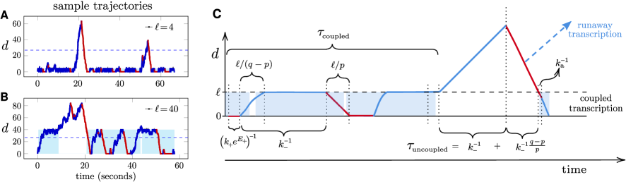
Figure S1: (A) A sample trajectory of distance $d$ between ribosome and RNAP as a function of time $t$, with $\ell=4$, $L=1000$, and all other parameters equivalent to those used in to generate Fig. 4. (B) A sample trajectory when the interaction distance is increased to $\ell=40$, relevant for example, if an intermediate protein such as NusG is involved in forming the ribosome-RNAP expressome complex. In (A) and (B), blue(red) segments indicate processing(stalled) RNAP. The light-blue shaded regions indicate bound ribosome-RNAP complexes. (C) Schematic description of distances and estimates of transition rates. These estimates assume that microstates within a macrostate has reached a local thermodynamic equilibrium in $(d,a,b)$-space.

Fig. S1A-B motivates us to lump all the different states of the system into four representative groups of microstates:

• The paused, separated state $(d>\ell,b=1)$.

• The processive, separated state $(d>\ell,b=0)$.

• The paused, proximal state, ($d\leq\ell,b=1$ and $a=1$ most of the time).

• The processive, proximal state, ($d\leq\ell,b=0$ and $a=1$ most of the time).

In the following, we call these four lumped states as “macrostates,” and the states within each macrostate as “microstates.” To derive the effective transition rates between macrostates, we assume that the microstates within each macrostate reach equilibrium much faster than the transitions between macrostates. The results are summarized in Figs. S1C and S2.

Traffic jam in associated, processive states.

As an example of a calculation of transition rates and velocities, consider the details of the expected velocity of a coupled, processive expressome. In this particular case, the ribosome and RNAP intermittently touch ($d=0$) each other. Therefore, they should have the same effective velocity $\bar{V}$. Suppose that the bound ribosome is slower than the processing RNAP, $p<q$. The average speed of the bound RNAP is thus limited by the speed of ribosome. However, the ribosome translocates at speed less than $p$ since it is occasionally blocked by the RNAP. The equilibrium probability that RNAP and ribosome are in contact ($d=0$) is given by

$$\pi(d=0\,|\,a=1,b=0)=\frac{1}{\sum_{k=0}^{\ell}(q/p)^{k}}.$$ (S18)

By finding the complementary probability that $0<d\leq\ell$, for which the ribosome can move forward with rate $p$, we find the expected expressome velocity

$$\mathbb{E}\left[{V}\,|\,a=1,b=0\right]=q\left[\frac{(q/p)^{\ell}-1}{(q/p)^{\ell+1}-1}\right].$$ (S19)

Since $q\sim 30$ codons/s and $p\leq 15$ codons/s, $q/p\sim 2$ and the relative slowdown is sensitive to $\ell$ with small $\ell$ resulting in a significant slowdown of the expressome.

Classification of different scenarios.

At equilibrium, if the average independent RNAP velocity $\bar{q}$ is smaller than $p$, the two machines will maintain a significant probability of proximity and coupling. However, if $p<\bar{q}$, the equilibrium ribosome-RNAP distance $d\to\infty$ and any interaction will vanish. Thus, we need only consider $p>\bar{q}$ and discuss the following scenarios:

1. The instantaneous speeds satisfy $p\geq q$. Then, the ribosome is always within close range of the RNAP and the system freely cycles among the four internal macrostates. We may assume that the binding and unbinding rates $k_{\rm a}$ and $k_{\rm d}$ are much larger than the pausing and unstalling rates $k_{-}$ and $k_{+}$.

2. The instantaneous speeds satisfy $p<q$ and the rate of uncoupling $k_{\rm d}$ is slower than the rate of pausing $k_{-}$. This system maintains an appreciable probability of being coupled. When the RNAP is bound and processive, the distance quickly increases until $d\approx\ell$. Because $k_{-}>k_{\rm d}$, the RNAP pauses often before it can break free from the ribosome. When the internal states become unbound, the ribosome can fall out of the interaction range $\ell$ and cannot immediately rebind. This gives rise to an effectively irreversible transition from a bound, processive state to an unbound, processive state. Rebinding can occur only after the RNAP again pauses, allowing the ribosome to catch up. Once this happens, the ribosome and RNAP will remain bound for a long time (since $E_{\rm a}$ is large).

3. The instantaneous speeds satisfy $p<q$, but the dissociation rate $k_{\rm d}$ is larger than the pausing rate $k_{-}$. This scenario is essentially the same as the previous one, with the only difference that the transition from the bound, processive state to an unbound processive state is fast and effectively irreversible.

These scenarios can be coarse-grained into different cyclic structures by grouping states that are connected by reversible reactions, as shown in Fig S2D-F. The effective transition rates are estimated based on the underlying dynamics.

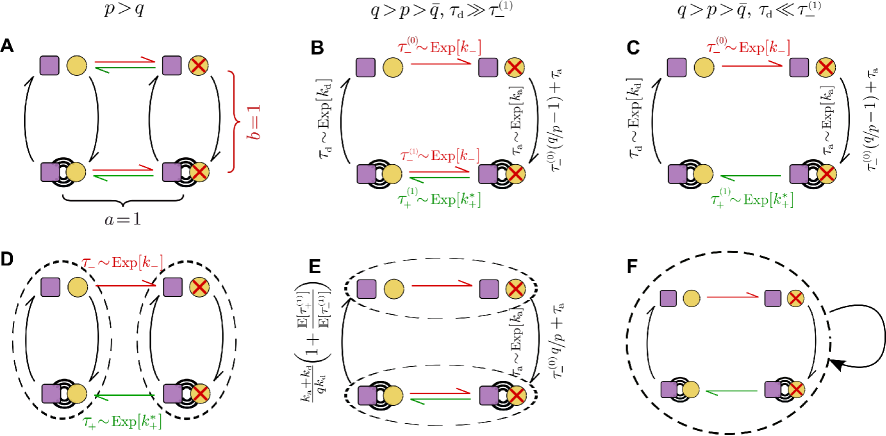
Figure S2: Coarse-grained states of the expressome. (A) A scenario in which binding and unbinding are relatively fast and that $p>q$ so that the ribosome is fast enough to fully allow binding. This case is rarely realized. (B) The limit in which binding is fast, but $\bar{q}<p<q$. In this case, when the ribosome and RNAP are unbound $(a=0)$, the ribosome falls out of the interaction range $\ell$ and cannot immediately rebind. The distance between the ribosome and the RNAP remains larger than $\ell$ until the RNAP pauses again and ribosome catches up. When the two machines are close, they effectively remain bound. Intermittent unbinding while in the processive state quickly leads to separation preventing binding until possibly after the next stall event. (C) Slow binding, fast unbinding regime that leads to only transient coupling. The slowdown of transcription is limited in this case. (D) The coarse-grained cyclic structure corresponding to the limit depicted in (A). Since binding and unbinding are fast, we can lump the “$a$ states” together as a single quasi-bound state reflecting an equilibrium weighting between bound and unbound. The effective rate constant out of this quasistate can be found by appropriate weighting of the two component rates. (E) represents the coarse-grained cyclic structure corresponding to the limit shown in (B). Due to strong binding, we assume that the transition from bound, $d\leq\ell$ states to unbound, $d>\ell$ states is slow relative to RNAP stalling/unstalling rates within bound states. Therefore, we group all the $a=1,d\leq\ell$ states together, and all the $a=0,\d{>}\ell$ states together. (F) Coarse-grained cyclic structure associated with the limit in (C). Scenario (C) is itself a strongly unidirectional cycle that we repeat to extract underlying distance traveled. The distributions of effective waiting times are indicated, e.g., $\tau_{+}^{(a)}\sim\textrm{Exp}[k_{+}^{*}]$ represents an exponentially distributed (with rate $k_{+}^{*}$) waiting time in the stalled, $a$-state before transitioning into a processing $a$-state. These rates are derived with an additional assumption that $\ell$ is small.

The waiting time distributions can be heuristically estimated as indicated in Fig. S1C and are indicated in Fig. S2. We can treat the cases depicted in Figs. S2D-F as repeated cycles marked by when ribosome and RNAP periodically meet each other. Therefore, in the large-$L$ limit, the effective velocities are approximately equal: $\overline{V}_{\rm rib}=\overline{V}_{\rm RNAP}\equiv\overline{V}$.

We analyze the mean and variance of the effective velocity by estimating the common random time $T$ to complete transcription and translation of all $L$ codons. First, define $\tau$ as the random time to traverse one internal-state cycle and $\overline{L}$ as the mean length traveled in one cycle. To complete a transcript of length $L$, $\sim L/\overline{L}$ cycles need to be completed. Each cycle can be considered independent and identically distributed. The total variance ${\rm Var}[T]$ and standard deviation $\sigma[T]$ of completion times is then given by

$${\rm Var}[T]\equiv(\sigma[T])^{2}\simeq{\rm Var}[\tau]\frac{L}{\overline{L}}$$ (S20)

and the effective velocities are

$$\overline{V}\pm\sigma[V]\sim\frac{L}{\mathbb{E}[T]\mp\sigma[T]}=\frac{\overline{L}}{\mathbb{E}[\tau]\mp\frac{\sigma[\tau]}{\sqrt{L/\overline{L}}}}.$$ (S21)

Thus, it is sufficient to characterize $\overline{L}$ and ${\rm Var}[\tau]$ to estimate $\overline{V}$ and its variation in each of the limits pictured in Figs. S2D-F

For the $p>q$ limit (Fig. S2D), the overall velocity is dictated by the velocity of the RNAP and the system can be approximated by a two-state model in which

$$\begin{cases}\displaystyle\overline{L}=q\mathbb{E}[\tau_{-}]=\frac{q}{k_{-}}\\ \displaystyle\mathbb{E}[\tau]=\mathbb{E}[\tau_{-}]+\mathbb{E}[\tau_{+}]=\frac{1}{k_{+}^{*}}+\frac{1}{k_{-}}\\ \displaystyle{\rm Var}[\tau]={\rm Var}[\tau_{-}]+{\rm Var}[\tau_{+}]=\frac{1}{{k_{+}^{*}}^{2}}+\frac{1}{k_{-}^{2}}.\end{cases}$$ (S22)

In the limit $\bar{q}<p<q$ and $\tau_{\rm d}\gg\tau^{(1)}_{-}$ (Fig. S2E), we apply Eq. S19 to find

$$\begin{cases}\displaystyle\overline{L}=q\frac{1}{k_{-}}+\frac{q}{k_{\rm d}}\left[\frac{(q/p)^{\ell}-1}{(q/p)^{\ell+1}-1}\right]\\ \displaystyle\mathbb{E}[\tau]=\mathbb{E}[\tau_{\rm a}]+\mathbb{E}[\tau^{(0)}_{-}]\frac{q}{p}+\mathbb{E}[\tau_{\rm d}^{(1)}]\frac{\mathbb{E}[\tau^{(1)}_{+}]+\mathbb{E}[\tau^{(1)}_{-}]}{\mathbb{E}[\tau^{(1)}_{-}]}\\ \displaystyle{\rm Var}[\tau]={\rm Var}[\tau_{\rm a}]+{\rm Var}[\tau^{(0)}_{-}]\frac{q^{2}}{p^{2}}+{\rm Var}[\tau_{\rm d}^{(1)}]\left(\frac{\mathbb{E}[\tau^{(1)}_{+}]+\mathbb{E}[\tau^{(1)}_{-}]}{\mathbb{E}[\tau^{(1)}_{-}]}\right)^{2}\end{cases}$$ (S23)

In the $q>p>\bar{q}$ and $\tau_{\rm d}\ll\tau^{(1)}_{-}$ limit (Fig. S2F), we also assume $q\gg k_{\rm a},k_{\rm d}$ to find

$$\begin{cases}\displaystyle\overline{L}=q\frac{1}{k_{-}}+\frac{q}{k_{\rm d}}\left[\frac{(q/p)^{\ell}-1}{(q/p)^{\ell+1}-1}\right]\\ \displaystyle\mathbb{E}[\tau]=\mathbb{E}[\tau_{\rm a}]+\mathbb{E}[\tau^{(0)}_{-}]\frac{q}{p}+\mathbb{E}[\tau_{\rm d}^{(1)}]+\mathbb{E}[\tau^{(1)}_{+}]\\ \displaystyle{\rm Var}[\tau]={\rm Var}[\tau_{\rm a}]+{\rm Var}[\tau^{(0)}_{-}]\frac{q^{2}}{p^{2}}+{\rm Var}[\tau_{\rm d}^{(1)}]+{\rm Var}[\tau^{(1)}_{+}]\end{cases}$$ (S24)

Estimation of the effective velocity and fraction of protected time.

It turns out that with realistic parameter values, our metrics are rather insensitive to the magnitudes of $k_{\rm a}$ and $k_{\rm d}$. Therefore, we focus on the cases $\tau_{\rm d}\gg\tau_{-}^{(1)}$ and $q\gg k_{\rm a}$ or $k_{\rm d}$. In the case $k_{\rm d}\ll k_{-}$ and $k_{\rm d}\ll k_{\rm a}$, the ribosome and RNAP are in molecular contact most of the time. For the sake of simplicity, we consider the extreme limit $E_{\rm a}\rightarrow\infty$. and simply evaluate the effective velocity for the coupled expressome. The mean/effective velocity $\overline{V}$ can be constructed using Eq. S23 and simplified to

$$\overline{V}\approx q\left[\frac{(q/p)^{\ell}-1}{(q/p)^{\ell+1}-1}\right]\frac{k_{+}^{*}}{k_{+}^{*}+k_{-}}.$$ (S25)

For sufficiently large $q$ and $\ell$, the coefficient $\left[\frac{(q/p)^{\ell}-1}{(q/p)^{\ell+1}-1}\right]\sim p/q$ and $\overline{V}\approx pk_{+}^{*}/(k_{+}^{*}+k_{-})$ as expected. Since $k_{+}^{*}\geq k_{+}$, the effective velocity has a lower bound

$$\overline{V}\geq\frac{pk_{+}}{k_{+}+k_{-}}\geq\frac{\bar{q}k_{+}}{k_{+}+k_{-}}.$$ (S26)

Estimation of the protected fraction.

Under the same assumption that $\bar{q}<p<q$, $\tau_{\rm d}\gg\tau_{-}^{(1)}$, it is possible to estimate the protected fraction by investigating the equilibrium distribution of distances $d$. Here, we need to separately discuss two scenarios as shown in Figs. S1A and B, respectively. The two different cases are characterized by the length of interaction $\ell$.

In the first case, $\ell/(q-p)\ll k_{-}^{-1}$. Consequently, in the bound, processive state, the ribosome-RNAP distance $d\approx\ell$ for the most of the time. In the second case, $\ell/(q-p)\gg k_{-}^{-1}$ and $\ell>\ell_{\rm p}$. Consequently, in the bound, processive state, the ribosome spends most of its time separated $0<d<\ell$. Only occasionally, $d=\ell$ before RNAP unpauses again and RNAP is able to break away from the lagging ribosome.

If the first case holds, unprotected states arise only when the system is unbound and $d>\ell$. Here, we consider a simple asymmetric random walk starting from $d=\ell$ that increases to $d+1$ with rate $q$ and decreases to $d-1$ with rate $p$. There are three stopping times that come into play. $\tau_{-1}$ is the first time $d_{t}=\ell-1$. $\tau_{\ell_{\rm p}}$ is the first time $d_{t}=\ell_{\rm p}$, and $\tau_{-}$ is the time to first RNAP pausing.

We heuristically estimate the probability that $\tau_{\ell_{\rm p}}<\tau_{-1}$, $\tau_{-}$ as well as the mean duration of exposure conditional on $\tau_{\ell_{\rm p}}<\tau_{-1},\tau_{-}$. The average of the largest distance $d_{\rm max}$ during the whole process is given by $(q-p)/k_{-}$. The standard deviation of $d_{\rm max}$ is determined by the square root of the average number of steps $\sqrt{(p+q)/k_{-}}$. Then, roughly $d_{\rm max}$ follows a normal distribution with mean $(q-p)/k_{-}$ and standard deviation $\sqrt{(p+q)/k_{-}}$. The probability that there is an unprotected duration is given by $\mathbb{P}(d_{\rm max}>\ell_{\rm p}-\ell)$. Due to the memoryless property of the exponential distribution, the average duration conditional on $d_{\rm max}>\ell_{\rm p}-\ell$ is essentially the same as the average duration of the whole uncoupled event $\frac{q}{pk_{-}}$. Therefore, and estimate of the mean protected time fraction is

$$\mathbb{E}[F_{T}]\sim 1-\frac{\frac{q}{pk_{-}}\mathbb{P}(d_{\rm max}>\ell_{\rm p}-\ell)}{\frac{q}{pk_{-}}+\frac{k_{\rm a}+k_{\rm d}}{qk_{\rm d}}\frac{k_{+}^{*}+k_{-}}{k_{+}^{*}}}\approx 1-\frac{\frac{q}{2pk_{-}}\left[1-\textrm{erf}\bigg{(}\frac{\ell_{\rm p}-\ell-(q-p)/k_{-}}{\sqrt{2(p+q)/k_{-}}}\bigg{)}\right]}{\frac{q}{pk_{-}}+\frac{k_{\rm a}+k_{\rm d}}{qk_{\rm d}}\frac{k_{+}^{*}+k_{-}}{k_{+}^{*}}}$$ (S27)

For the second case, $\ell/(q-p)\gg k_{-}^{-1}$ and $\ell>\ell_{\rm p}$, we are primarily interested in the bound states since as $\ell$ increases, the chances that unbound states arise decrease. However, since $\ell>\ell_{\rm p}$, even in the bound state, there is a chance that $d>\ell_{\rm p}$. Estimation of the probability that the exposed state is visited follows a similar argument as the previous calculation where we examined the distribution of $d_{\rm max}$. The main difference is that the asymptotic distribution of $d_{\rm max}$ is now different from the normal distribution due to $\ell>\ell_{\rm p}$. This also changes the duration of exposed states. For simplicity, we consider only the $\ell\to\infty$ limit to find

$$\mathbb{E}[F_{T}]\sim 1-\frac{qk_{+}^{*}}{2(qk_{+}^{*}+pk_{-})}\left[1-\textrm{erf}\bigg{(}\frac{\ell_{\rm p}-(q-p)/k_{-}}{\sqrt{2(p+q)/k_{-}}}\bigg{)}\right].$$ (S28)

Our preliminary analyses suggest that in the short interaction range limit, the quantity $\frac{\ell_{\rm p}-\ell-(q-p)/k_{-}}{\sqrt{2(p+q)/k_{-}}}$ plays a significant role in determining $F_{T}$, while in the long interaction range limit, $\frac{\ell_{\rm p}-(q-p)/k_{-}}{\sqrt{2(p+q)/k_{-}}}$ plays a similar role.

S5 Variability of the protected-time fraction $F_{T}$

Fig. 4E plotted only the expected protected fraction. Since $F_{T}$ we generated via the full stochastic simulation, the variability of $F_{T}$ is also of interest. Here, we plot the standard deviation $\sigma[F_{T}]$ versus simulated values of $F_{T}$ to show that it agrees qualitatively well with $\sqrt{\mathbb{E}[F_{T}]\big{(}1-\mathbb{E}[F_{T}]\big{)}}$.

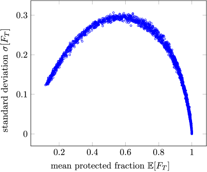
Figure S3: Standard deviation $\sigma[F_{T}]$ as a function of $\mathbb{E}[F_{T}]$ computed using different values of $(p,q)$. All other parameter values are those used in Fig. 4E.

S6 Effects of interaction length $\ell$

The interaction length $\ell$ is one factor that influences coupling-induced slowdown, as indicated by Eq. S25. The interaction length is not a significant contributing factor to slowdown because the factor $\left[\frac{(q/p)^{\ell}-1}{(q/p)^{\ell+1}-1}\right]$ is already $\sim 1$ when $\ell\sim 5$. This factor is small only when $\ell\approx 0$. Since $\ell$ takes on integer values this slowdown factor never really really becomes very small. On the other hand, the interaction length $\ell$ also dictates the distribution of $d$ conditioned on $a=1$. For example, if $\ell/p\gg k_{-}$, then the most probable distance between ribosome and RNAP will be $d=\ell$.

We have found an interesting “bifurcation” in effective velocity and mean protected times when the interaction distance $\ell>\ell_{\rm p}=27$, the mRNA footprint length of a transcription terminator such as Rho. If $\ell<\ell_{\rm p}$, protection by the ribosome can be thought of as being purely due to steric exclusion effects; once $d>\ell_{\rm p}$, protection is lost. However, if $\ell>\ell_{\rm p}$ one can consider a “binding-based” protection that requires either $d\leq\ell_{p}$ or $a=1$ for protection. In this case, even if $\ell>d>\ell_{\rm p}$, there can be protection due to binding-mediated conformational shielding of the intervening mRNA that makes it inaccessible to termination factors. The different criteria for protection lead to drastically different levels of protection provided by the ribosome, as shown in Fig. S4.

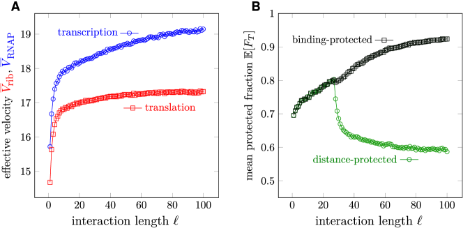
Figure S4: Functional consequences of varying interaction length $\ell$. Unspecified parameters are the same as those used in Fig. 4. (A) Effective velocities as a function of $\ell$. Note the sharp drop when $\ell\rightarrow 0$. (B) Bifurcation of $\mathbb{E}[F_{T}]$ as a function of $\ell$ due to different definitions of protection. Other parameters are the same as those used in the Fig. 4. When $\ell<\ell_{\rm p}=27$, the two definitions of $F_{T}$ agree. When $\ell>\ell_{\rm p}$, the $\mathbb{E}[F_{T}]$ based purely distance is drastically lower as $\ell$ increases.