Measuring differential flow angle fluctuations in relativistic nuclear collisions

Abstract

Recently studies of the differential nature of the flow angle fluctuations, known as event plane angular decorrelation, indicated that measurements that assume a common symmetry plane may need to consider the flow angle fluctuations effect. Using the HIJING and AMPT models, it is shown that the flow angle fluctuations measurements, obtained with the two- and three-subevents correlation method, could have significant non-flow effects associated with long- and short-range non-flow correlations. The current study demonstrates the four-subevents cumulant methods’ ability to reduce the non-flow effects. It is further argued that the measurements using the four-subevents correlation method can be used to provide accurate quantification of the differential flow angle fluctuations.

I Introduction

Studies at the Large Hadron Collider (LHC) and the Relativistic Heavy Ion Collider (RHIC) aim to create and study the properties of the deconfined nuclear medium named quark-gluon plasma (QGP) Shuryak (1978, 1980); Muller et al. (2012). In non-central collisions, the medium created by the participant (nucleons that experience at least one collision) interactions will experience a hydrodynamic expansion with an initial geometry defined by the participant distribution, with event-by-event fluctuations. In a hydrodynamic evolution, the created medium’s pressure gradients transform the initial state’s spatial anisotropies into final-state momentum anisotropies. Accordingly, the azimuthal distributions of the particles created in the collisions can be analyzed with a Fourier expansion Voloshin and Zhang (1996); Poskanzer and Voloshin (1998):

$$\dfrac{dN}{d\varphi} \propto 1+\sum_{n=1}^{\infty}2v_{n}\cos\left[n(\varphi-\Psi^{\rm RP})\right],$$ (1)

where $\varphi$ illustrates the azimuthal angle of a the particle, $v_{n}$ is the n^th order Fourier coefficients, and $\Psi^{\rm RP}$ is the direction of the reaction plane. The n^th Fourier coefficients can be provided as:

$$v_{n}=\langle\cos[n(\varphi-\Psi_{n})]\rangle\,,$$ (2)

where $\Psi_{n}$ is the flow angles event plan, $\textit{v}_{1}$ is called directed flow, $\textit{v}_{2}$ is the elliptic flow, and $\textit{v}_{3}$ is the triangular flow, etc.

While $v_{n}$ fluctuations and the effect of their variance on different methods for measuring $v_{n}$ have been studied extensively Voloshin et al. (2010); Heinz and Snellings (2013), flow angle fluctuations (i.e., flow decorrelations) have recently found attention Qiu and Heinz (2011); Teaney and Yan (2011); Gardim et al. (2012); Teaney and Yan (2012); Jia and Mohapatra (2013); Jia (2013); Qiu and Heinz (2012); Ollitrault and Gardim (2013); Gardim et al. (2013) both theoretically and experimentally. The flow angles $\Psi_{n}$ fluctuations (decorrelations) depend on transverse momentum ($p_{T}$) Gardim et al. (2013, 2018); Zhao et al. (2017); Bożek (2018); Barbosa et al. (2021) and pseudorapidity ($\eta$) Bozek et al. (2011); Jia and Huo (2014); Pang et al. (2015, 2016); Khachatryan et al. (2015); Bozek and Broniowski (2018); Cimerman et al. (2021) leading to additional fluctuations between the integrated event plane and the $p_{T}$ or $\eta$ differential event plane. Such correlations can lead to a factorization breaking (i.e., the two-particle angular correlations do not factorize into a product of single-particle flow coefficients). The $p_{T}$ and $\eta$ dependence of the flow angles $\Psi_{n}$ fluctuations are studied using two-particle correlations Bozek et al. (2011); Jia and Huo (2014) and, recently, four-particle correlations Nielsen (2020); Aaboud et al. (2018); ALI (2022); Bozek and Samanta (2022). The longitudinal and transverse momentum flow angle fluctuations give essential insight into the nature of the initial state event-by-event fluctuations of the heavy-ion collisions. Therefore, studying the differential flow angle fluctuations can reflect its impact on the measurements that assume a common symmetry plane.

The flow angle fluctuations are measured using the two- and four-particle correlations Bozek et al. (2011); Jia and Huo (2014); Bozek and Samanta (2022). The two- and four-particle correlations are susceptible to long-range non-flow correlations (e.g., jets in a dijet event) and short-range non-flow correlations (e.g., resonance decays, Bose-Einstein correlation, and fragments of individual jets). Such non-flow correlations usually involve a few particles from one or more $\eta$ regions. The non-flow effects are usually reduced by correlating particles from two or more subevents divided in pseudorapidity. Therefore, a more detailed study of the influence of non-flow effects on these observables is required before interpreting the experimental measurements. Event generators such as the HIJING model Wang and Gyulassy (1991); Gyulassy and Wang (1994), which contain only non-flow correlations, are an ideal testing ground for estimating the influence of non-flow on the four-particle correlations, which are part of the focus of this paper.

The present study investigates the non-flow effects on the flow angles $\Psi_{n}$ fluctuations measurements and its $p_{T}$ dependence using the HIJING Wang and Gyulassy (1991); Gyulassy and Wang (1994) model. In addition, this study used the A Multi-Phase Transport (AMPT) Lin et al. (2005) model to investigate the proposed observables, which have been shown to have minimal non-flow effects, on measurements of the $p_{T}$ dependence of the flow angles $\Psi_{n}$ fluctuations. The models and analysis method used are given in II. The results and discussion are presented in section III. The conclusions of this work are summarized in section IV.

II Methodology

II.1 Models

The present analysis is performed with events simulated by HIJING Wang and Gyulassy (1991); Gyulassy and Wang (1994) and the AMPT (v2.26t9b) Lin et al. (2005) models for Au+Au (Pb+Pb) collisions at $\sqrt{s_{NN}}$ = 200(5020) GeV. In both models, charged particles with $0.2<p_{T}<5.0$ GeV/$c$, and $|\eta|<5.0$ were selected for analysis. The HIJING model emphasizes the effects of mini-jets non-flow correlations, while the AMPT model is used to investigate the flow angle fluctuations. The AMPT model, which is employed to study the physical process in relativistic heavy-ion collisions Lin et al. (2005); Ma and Lin (2016); Ma (2013, 2014); Bzdak and Ma (2014); Nie et al. (2018); Haque et al. (2019); Zhao et al. (2020); Bhaduri and Chattopadhyay (2010); Nasim et al. (2010); Xu and Ko (2011a); Magdy et al. (2020a); Guo et al. (2019); Magdy et al. (2020b); Magdy (2022a). The AMPT model includes several important model elements: (i) an initial partonic state provided by the HIJING model Wang and Gyulassy (1991); Gyulassy and Wang (1994), with the HIJING model parameters, $a=0.55$ and $b=0.15$ GeV^-2 are used for the Lund string fragmentation function $f(z)\propto z^{-1}(1-z)^{a}\exp(-b~{}m_{\perp}^{2}/z)$, where $z$ represents the light-cone momentum fraction of the yielded hadron of transverse mass $m_{\perp}$ about that of the fragmenting string. Also, (ii) partonic scattering with a cross-section,

$$\sigma_{pp} = \dfrac{9\pi\alpha^{2}_{s}}{2\mu^{2}},$$ (3)

where $\mu$ is the screening mass and $\alpha_{s}$ represents the coupling constant of the QCD. The partonic scattering with cross-section $\sigma_{pp}$ drives the expansion dynamics Zhang (1998); (iii) the hadronization process through coalescence followed by the hadronic interactions Li and Ko (1995). In the current work, the $\alpha_{s}$ and $\mu$ are fixed to 0.47 and 3.41 $fm^{-1}$ Xu and Ko (2011b) respectively.

II.2 Analysis Method

The events generated were analyzed using the two- and multi-particle correlations given via the use of the subevents cumulant methods Jia et al. (2017); Huo et al. (2018); Zhang et al. (2019); Magdy et al. (2020a). The observables discussed in this work can be given in terms of the flow vectors as;

$$Q_{n,X_{j}} = \sum_{i}e^{\mathit{i}n\phi_{i}},$$ (4)

where $\phi_{i}$ is the azimuthal angle of the $\mathit{i}^{th}$ particle in the $X_{j}$ subevent.

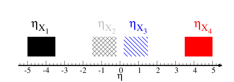
Figure 1: The $\eta$ ranges for the subevents used in this work.

In Fig. 1, events are partitioned into four subevents, $\eta_{X_{1}}$ and $\eta_{X_{4}}$ as an integrated flow vector and $\eta_{X_{2}}$ and $\eta_{X_{3}}$ as a differential flow vector. The current work contains two assumptions; first the two integrated(differential) event planes are equivalent (i.e., $\psi_{X_{1},n}\sim\psi_{X_{4},n}\sim\psi_{n}$ and $\psi^{d}_{X_{2}}~{}\sim~{}\psi^{d}_{X_{3}}~{}\sim~{}\psi_{d,n}$). Second, non-flow effects are very small for the two-particle correlations with a large $\eta$ gap.

The two-particle correlations can be given as;

$$\langle 2\rangle_{X_{1}X_{1}} = e^{\mathit{i}n(\phi_{1,X_{1}}-\phi_{2,X_{1}})}\equiv\dfrac{Q_{n,X_{1}}Q^{*}_{n,X_{1}}-M_{X_{1}}}{M_{X_{1}}(M_{X_{1}}-1)},$$ (5)

$$\langle 2\rangle_{X_{1}X_{3}} = e^{\mathit{i}n(\phi_{1,X_{1}}-\phi_{2,X_{3}})}\equiv\dfrac{Q_{n,X_{1}}Q^{*}_{n,X_{3}}}{M_{X_{1}}M_{X_{3}}},$$

where $M_{X}$ is the number of particles in subevent $X$.

The overall two-particle correlations can be rewritten as;

$$\langle\langle 2\rangle\rangle \sim \langle\langle 2\rangle\rangle_{g}+\delta_{2}$$ (6)

where $\langle\langle~{}\rangle\rangle$ refer to average over all tracks and average over all events, $\delta_{2}\thicksim\delta_{2,short}+\delta_{2,long}$ is non-flow from two-particle correlations and $\langle\langle 2\rangle\rangle_{g}$ is the two-particle flow correlations (i.e., determined by the geometry of the collision system). Note that short-range non-flow can be reduced using the subevents methods with $\eta$ gap Magdy (2022b).

The four-particle correlations can be given using the two-subevents as;

$$\langle 4\rangle_{T_{1},X_{1}X_{3}} = e^{\mathit{i}n(\phi_{1,X_{1}}+\phi_{1,X_{1}}-\phi_{3,X_{3}}-\phi_{4,X_{3}})}$$

$$\equiv \dfrac{(Q^{2}_{n,X_{1}}-Q_{2n,X_{1}})(Q^{2}_{n,X_{3}}-Q_{2n,X_{3}})^{*}}{M_{X_{1}}(M_{X_{1}}-1)M_{X_{3}}(M_{X_{3}}-1)},$$

$$\langle 4\rangle_{T_{2},X_{1}X_{3}} = e^{\mathit{i}n(\phi_{1,X_{1}}+\phi_{1,X_{3}}-\phi_{3,X_{1}}-\phi_{4,X_{3}})}$$

$$\equiv \dfrac{(Q^{2}_{n,X_{1}}-M_{X_{1}})(Q^{2}_{n,X_{3}}-M_{X_{3}})^{*}}{M_{X_{1}}(M_{X_{1}}-1)M_{X_{3}}(M_{X_{3}}-1)},$$

where $T_{1,2}$ represent type $I$, and $II$ for the four-particle correlations.

The four-particle correlations can be given using the three-subevents as;

$$\langle 4\rangle_{T_{1},X_{1}X_{2}X_{3}} = e^{\mathit{i}n(\phi_{1,X_{1}}+\phi_{1,X_{1}}-\phi_{3,X_{2}}-\phi_{4,X_{3}})}$$

$$\equiv \dfrac{(Q^{2}_{n,X_{1}}-Q_{2n,X_{1}})(Q_{n,X_{2}}Q_{n,X_{3}})^{*}}{M_{X_{1}}(M_{X_{1}}-1)M_{X_{2}}M_{X_{3}}},$$

$$\langle 4\rangle_{T_{2},X_{1}X_{2}X_{3}} = e^{\mathit{i}n(\phi_{1,X_{1}}+\phi_{1,X_{2}}-\phi_{3,X_{1}}-\phi_{4,X_{3}})}$$

$$\equiv \dfrac{(Q^{2}_{n,X_{1}}-M_{X_{1}})Q_{n,X_{2}}Q^{*}_{n,X_{3}}}{M_{X_{1}}(M_{X_{1}}-1)M_{X_{2}}M_{X_{3}}}.$$

The four-particle correlations can be given using the four-subevents as;

$$\langle 4\rangle_{T_{1},X_{1}X_{2}X_{3}X_{4}} = e^{\mathit{i}n(\phi_{1,X_{1}}+\phi_{1,X_{2}}-\phi_{3,X_{3}}-\phi_{4,X_{4}})}$$

$$\equiv \dfrac{(Q_{n,X_{1}}Q^{*}_{n,X_{3}})(Q_{n,X_{2}}Q^{*}_{n,X_{4}})}{M_{X_{1}}M_{X_{2}}M_{X_{3}}M_{X_{4}}},$$

$$\langle 4\rangle_{T_{2},X_{1}X_{2}X_{3}X_{4}} = e^{\mathit{i}n(\phi_{1,X_{1}}+\phi_{1,X_{2}}-\phi_{4,X_{4}}-\phi_{3,X_{3}})}$$

$$\equiv \dfrac{(Q_{n,X_{1}}Q^{*}_{n,X_{4}})(Q_{n,X_{2}}Q^{*}_{n,X_{3}})}{M_{X_{1}}M_{X_{2}}M_{X_{3}}M_{X_{4}}}.$$

Note that the integrated $\langle 4\rangle_{T_{1},X_{1}X_{2}X_{3}X_{4}}$ and $\langle 4\rangle_{T_{2},X_{1}X_{2}X_{3}X_{4}}$ are equivalent by construction.

In general the different contributions to the four-particle correlations Jia et al. (2017) can be given as:

$$\langle\langle 4\rangle\rangle \sim \langle\langle 4\rangle\rangle_{g}+\delta_{4}+\delta_{2},$$ (13)

where $\delta_{4}$ is non-flow from four-particle correlations and $\langle\langle 4\rangle\rangle_{g}$ is the four-particle flow correlations.

Note that using type-I two-, three- and four-subevets with $\eta$ gaps, most of non-flow in the four-particle correlations is reduced. In contrast, type-II will contain more non-flow Jia et al. (2017). The latter can be reduce by subtracting the two-particle correlations Eq. 5 in the $k$-particle cumulants Jia et al. (2017). The four-particle cumulants are given as:

$$C_{T_{1},X_{1}X_{3}} = \langle\langle 4\rangle\rangle_{T_{1},X_{1}X_{3}}-2\langle\langle 2\rangle\rangle_{X_{1}X_{3}}\langle\langle 2\rangle\rangle_{X_{1}X_{3}},$$ (14)

$$C_{T_{1},X_{1}X_{2}X_{3}} = \langle\langle 4\rangle\rangle_{T_{1},X_{1}X_{2}X_{3}}-2\langle\langle 2\rangle\rangle_{X_{1}X_{2}}\langle\langle 2\rangle\rangle_{X_{1}X_{3}},$$

$$C_{T_{1},X_{1}X_{2}X_{3}X_{4}} = \langle\langle 4\rangle\rangle_{T_{1},X_{1}X_{2}X_{3}X_{4}}-\langle\langle 2\rangle\rangle_{X_{1}X_{3}}\langle\langle 2\rangle\rangle_{X_{2}X_{4}},$$

$$- \langle\langle 2\rangle\rangle_{X_{1}X_{4}}\langle\langle 2\rangle\rangle_{X_{1}X_{3}}$$

$$C_{T_{2},X_{1}X_{3}} = \langle\langle 4\rangle\rangle_{T_{2},X_{1}X_{3}}-\langle\langle 2\rangle\rangle_{X_{1}X_{1}}\langle\langle 2\rangle\rangle_{X_{3}X_{3}}$$

$$- \langle\langle 2\rangle\rangle_{X_{1}X_{3}}\langle\langle 2\rangle\rangle_{X_{1}X_{3}},$$

$$C_{T_{2},X_{1}X_{2}X_{3}} = \langle\langle 4\rangle\rangle_{T_{2},X_{1}X_{2}X_{3}}-\langle\langle 2\rangle\rangle_{X_{1}X_{1}}\langle\langle 2\rangle\rangle_{X_{2}X_{3}}$$

$$- \langle\langle 2\rangle\rangle_{X_{1}X_{2}}\langle\langle 2\rangle\rangle_{X_{1}X_{3}},$$

$$C_{T_{2},X_{1}X_{2}X_{3}X_{4}} = \langle\langle 4\rangle\rangle_{T_{2},X_{1}X_{2}X_{4}X_{3}}-\langle\langle 2\rangle\rangle_{X_{1}X_{3}}\langle\langle 2\rangle\rangle_{X_{2}X_{4}}$$

$$- \langle\langle 2\rangle\rangle_{X_{1}X_{4}}\langle\langle 2\rangle\rangle_{X_{2}X_{3}}.$$

Note that the integrated $C_{T_{1},X_{1}X_{2}X_{3}X_{4}}$ and $C_{T_{2},X_{1}X_{2}X_{3}X_{4}}$ are equivalent by construction.

II.2.1 The flow angle fluctuations

The differential/integrated two-particle correlations via the two-subevents method with $\eta$ gap can be given as;

$$\langle\langle 2\rangle\rangle_{X_{1}X^{d}_{3}} \sim \langle v_{n,X_{1}}v_{n,d,X_{3}}cos\left(n\left(\psi_{n,X_{1}}-\psi_{n,d,X_{3}}\right)\right)\rangle$$ (16)

$$\sim \langle v_{d,n}v_{n}cos\left(n\left(\psi_{n,d}-\psi_{n}\right)\right)\rangle,$$

$$\langle\langle 2\rangle\rangle_{X^{d}_{1}X^{d}_{3}} \sim \langle v_{n,d,X_{1}}v_{n,d,X_{3}}cos\left(n\left(\psi_{n,d,X_{1}}-\psi_{n,d,X_{3}}\right)\right)\rangle$$ (17)

$$\sim \langle v_{d,n}v_{d,n}\rangle.$$

Also the type-I differential four-particle correlations are given as;

$$\langle\langle 4\rangle\rangle_{T1,X_{1}X^{d}_{3}} \sim \langle v^{2}_{n,X_{1}}v^{2}_{n,d,X_{3}}$$ (18)

$$cos\left(2n\left(\psi_{n,X_{1}}-\psi_{n,d,X_{3}}\right)\right)\rangle$$

$$\sim \langle v^{2}_{n}v^{2}_{n,d}cos\left(2n\left(\psi_{n}-\psi_{n,d}\right)\right)\rangle,$$

$$\langle\langle 4\rangle\rangle_{T1,X_{1}X^{d}_{2}X^{d}_{3}} \sim \langle v^{2}_{n,X_{1}}v_{n,d,X_{2}}v_{n,d,X_{3}}$$ (19)

$$cos\left(n\left(\psi_{n,X_{1}}-\psi_{n,d,X_{2}}\right)\right)$$

$$cos\left(n\left(\psi_{n,X_{1}}-\psi_{n,d,X_{3}}\right)\right)\rangle$$

$$\sim \langle v^{2}_{n}v^{2}_{n,d}cos\left(2n\left(\psi_{n}-\psi_{n,d}\right)\right)\rangle,$$

$$\langle\langle 4\rangle\rangle_{T1,X_{1}X^{d}_{2}X^{d}_{3}X_{4}} \sim \langle v_{n,X_{1}}v_{n,d,X_{2}}v_{n,d,X_{3}}v_{n,X_{4}}$$ (20)

$$cos\left(n\left(\psi_{n,X_{1}}-\psi_{n,d,X_{3}}\right)\right)$$

$$cos\left(n\left(\psi_{n,d,X_{2}}-\psi_{n,X_{4}}\right)\right)\rangle$$

$$\sim \langle v^{2}_{n}v^{2}_{n,d}cos\left(2n\left(\psi_{n}-\psi_{n,d}\right)\right)\rangle.$$

The type-II differential four-particle correlations are given as;

$$\langle\langle 4\rangle\rangle_{T2,X_{1}X^{d}_{3}} \sim \langle v^{2}_{n,X_{1}}v^{2}_{n,d,X_{3}}$$ (21)

$$cos\left(n\left(\psi_{n,X_{1}}-\psi_{n,X_{1}}\right)\right)\rangle$$

$$cos\left(n\left(\psi_{n,d,X_{3}}-\psi_{n,d,X_{3}}\right)\right)\rangle$$

$$+ \delta_{2,X_{1}}\delta_{2,X_{3}}$$

$$\sim \langle v^{2}_{n}v^{2}_{n,d}\rangle+\delta_{2,X_{1}}\delta_{2,X_{3}},$$

$$\langle\langle 4\rangle\rangle_{T2,X_{1}X^{d}_{2}X^{d}_{3}} \sim \langle v^{2}_{n,X_{1}}v_{n,d,X_{2}}v_{n,d,X_{3}}$$ (22)

$$cos\left(n\left(\psi_{n,X_{1}}-\psi_{n,X_{1}}\right)\right)$$

$$cos\left(n\left(\psi_{n,d,X_{2}}-\psi_{n,d,X_{3}}\right)\right)\rangle$$

$$+ \delta_{2,X_{1}}$$

$$\sim \langle v^{2}_{n}v^{2}_{n,d}\rangle+\delta_{2,X_{1}},$$

$$\langle\langle 4\rangle\rangle_{T2,X_{1}X^{d}_{2}X^{d}_{3}X_{4}} \sim \langle v_{n,X_{1}}v_{n,d,X_{2}}v_{n,d,X_{3}}v_{n,X_{4}}$$ (23)

$$cos\left(n\left(\psi_{n,X_{1}}-\psi_{n,X_{4}}\right)\right)$$

$$cos\left(n\left(\psi_{n,d,X_{2}}-\psi_{n,d,X_{3}}\right)\right)\rangle$$

$$\sim \langle v^{2}_{n}v^{2}_{n,d}\rangle.$$

• The differential flow angle fluctuations using the two-particles correlations and two-subevents can be given as:

  $$r_{2}\{2,2S\}(p_{T}) = \dfrac{\langle\langle 2\rangle\rangle_{X_{1}X^{d}_{3}}}{\sqrt{\langle\langle 2\rangle\rangle_{X^{d}_{1}X^{d}_{3}}\langle\langle 2\rangle\rangle_{X_{1}X_{3}}}}$$ (24)

  $$\sim cos\left(n\left(\psi_{n,d}-\psi_{n}\right)\right)$$

• The differential flow angle fluctuations using the four-particles and two-subevents can be given as:

  $$r_{2}\{4,2S\}(p_{T}) = \dfrac{\langle\langle 4\rangle\rangle_{T_{1},X_{1}X^{d}_{3}}}{\langle\langle 4\rangle\rangle_{T_{2},X_{1}X^{d}_{3}}}$$ (25)

  $$\sim \dfrac{\langle v^{2}_{n}v^{2}_{n,d}cos\left(2n\left(\psi_{n}-\psi_{n,d}\right)\right)\rangle}{\langle v^{2}_{n}v^{2}_{n,d}\rangle+\delta_{2,X_{1}}\delta_{2,X_{3}}}.$$

• The differential flow angle fluctuations using the four-particle and three-subevents can be given as:

  $$r_{2}\{4,3S\}(p_{T}) = \dfrac{\langle\langle 4\rangle\rangle_{T_{1},X_{1}X^{d}_{2}X^{d}_{3}}}{\langle\langle 4\rangle\rangle_{T_{2},X_{1}X^{d}_{2}X^{d}_{3}}}$$ (26)

  $$\sim \dfrac{\langle v^{2}_{n}v^{2}_{n,d}cos\left(2n\left(\psi_{n}-\psi_{n,d}\right)\right)\rangle}{\langle v^{2}_{n}v^{2}_{n,d}\rangle+\delta_{2,X_{1}}}.$$

• The differential flow angle fluctuations using the four-particle and four-subevents can be given as:

  $$r_{2}\{4,4S\}(p_{T}) = \dfrac{\langle\langle 4\rangle\rangle_{T_{1},X_{1}X^{d}_{2}X^{d}_{3}X_{4}}}{\langle\langle 4\rangle\rangle_{T_{2},X_{1}X^{d}_{2}X^{d}_{3}X_{4}}}$$ (27)

  $$\sim \dfrac{\langle v^{2}_{n}v^{2}_{n,d}cos\left(2n\left(\psi_{n}-\psi_{n,d}\right)\right)\rangle}{\langle v^{2}_{n}v^{2}_{n,d}\rangle}$$

  $$\sim \langle cos\left(2n\left(\psi_{n}-\psi_{n,d}\right)\right)\rangle$$

III Results and discussion

The reliability of the extracted flow angles $\Psi_{n}$ fluctuations can be influenced by possible short- and long-range non-flow contributions to the two- and four-particle correlators used for the extractions. Therefore, it is informative to consider a figure of merit for these contributions to the four-particle correlations.

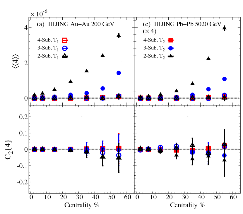
Figure 2: The centrality dependence of the four-particle correlations panels and the four-particle cumulant for Au+Au at $\sqrt{\textit{s}_{NN}}~{}=$ 200 GeV panels (a) and (b) and for Pb+Pb at $\sqrt{\textit{s}_{NN}}~{}=$ 5020 GeV from the HIJING model using the two-, three-, and four-subevents correlation methods.

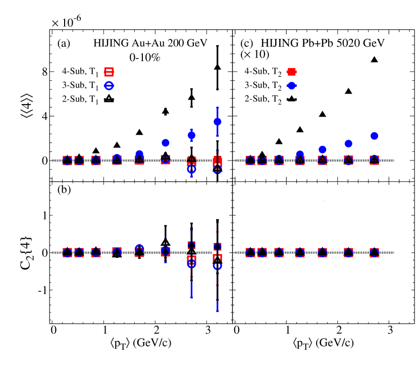
Figure 3: The 0-10% central $p_{T}$ dependence of the four-particle correlations panels and the four-particle cumulant for Au+Au at $\sqrt{\textit{s}_{NN}}~{}=$ 200 GeV panels (a) and (b) and for Pb+Pb at $\sqrt{\textit{s}_{NN}}~{}=$ 5020 GeV from the HIJING model using the two-, three-, and four-subevents correlation methods.

The non-flow effects on the (I) the four-particle correlations ($\langle\langle 4\rangle\rangle$) and (II) four-particle cumulant ($C_{2}\{4\}$) are shown in Figs. 2 and 3. The results are presented for Au+Au at $\sqrt{\textit{s}_{NN}}~{}=$ 200 GeV and Pb+Pb at $\sqrt{\textit{s}_{NN}}~{}=$ 5020 GeV from the HIJING model using the two-, three-, and four-subevents methods. The HIJING model results in Fig. 2 panels (a) and (c) show the centrality dependence of the $\langle\langle 4\rangle\rangle$. The type-I (all subevents) and type-II (four-subevents) $\langle\langle 4\rangle\rangle$ are much reduced, indicating little if any non-flow effects. In contrast, the two- and the three-subevents type-II $\langle\langle 4\rangle\rangle$ show a strong centrality dependence indicating non-flow effects from the $\langle\langle 2\rangle\rangle$ as pointed out in Eqs. 13, 21, and 22. The difference in values between the two presented energies is expected to be related to the multiplicity difference at the same centrality. In addition, the $C_{2}\{4\}$, which subtracts the two-particle correlations ( panels (b) and (d)) are shown to be zero indicating their ability to reduce non-flow effects. These results are compatible with other investigations Huo et al. (2018); Zhang et al. (2021).

The $\langle p_{T}\rangle$ dependence of the $\langle\langle 4\rangle\rangle$ for 0-10% central collisions are given in Fig. 3 (panels (a) and (c)). My results show that type-I (all subevents) and type-II (four-subevents) $\langle\langle 4\rangle\rangle$ are much reduced, indicating small non-flow effects. The two- and the three-subevents type-II $\langle\langle 4\rangle\rangle$ show a strong $\langle p_{T}\rangle$ dependence indicating that non-flow effects in the HIJING model are $\langle p_{T}\rangle$ dependent. As pointed out in Fig. 2 the $C_{2}\{4\}$ which subtracts the two-particle correlations (panels (b) and (d)) show little if any non-flow correlations.

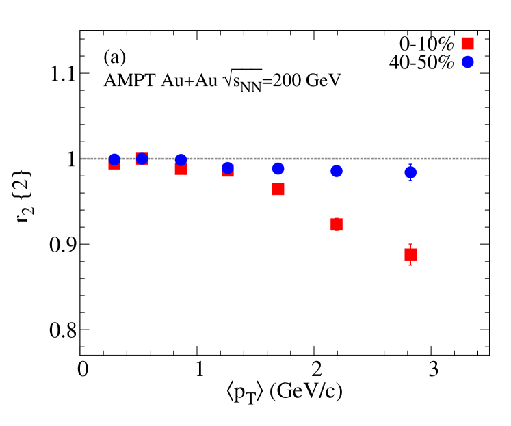
Figure 4: The $\langle p_{T}\rangle$ dependence of the $r_{2}\{2\}$($p_{T}$) correlator for 0-10% and 40-50% central collisions for Au+Au at $\sqrt{\textit{s}_{NN}}~{}=$ 200 GeV from the AMPT model.

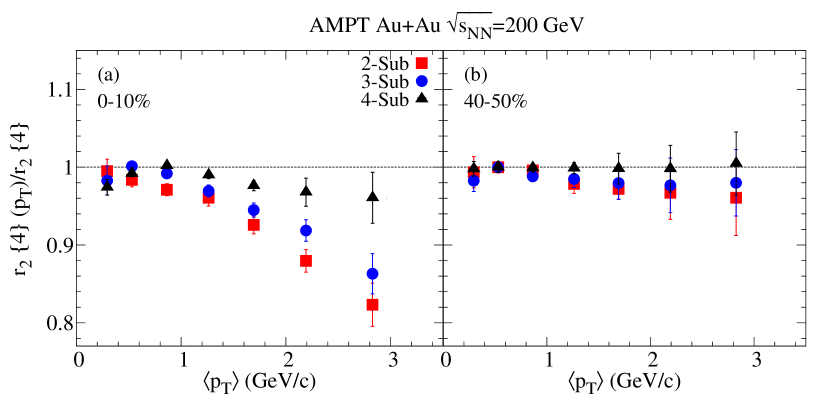
Figure 5: The $\langle p_{T}\rangle$ dependence of the normalized $r_{2}\{4\}$($p_{T}$) correlator using the two-, three-, and four-subevents for 0-10% (a) and 40-50% (b) central collisions for Au+Au at $\sqrt{\textit{s}_{NN}}~{}=$ 200 GeV from the AMPT model.

In this work, the HIJING model is used as a testing ground for non-flow effects on the $\langle\langle 4\rangle\rangle$ that are an essential part of $r_{2}\{4\}$. The results show that the two- and three-subevents results are contaminated by non-flow effects, which increase with centrality and $\langle p_{T}\rangle$. Such an effect could have an impact on the recent ALICE measurements ALI (2022) which use the two-subevents method with a small $\eta$ gap. In contrast, the HIJING model results in Figs. 2 and 3 suggest that the four-subevents cumulant method reduces the non-flow effects to less than 0.5%, albeit model dependent. Experimental measurements of comparable magnitude would, of course, be challenging to interpret. Although the four-subevents cumulant method is statistically demanding and often requires a wide $\eta$ acceptance, such a study can be achieved in the STAR experiment at RHIC Llope (1997) via the the STAR Event Plane Detector (EPD) Adams et al. (2020).

Figure 4 compares the $\langle p_{T}\rangle$ dependence of the two-particle $r_{2}\{2\}$ for 0-10% and 40-50% central collisions for Au+Au at $\sqrt{\textit{s}_{NN}}~{}=$ 200 GeV from the AMPT model. The results indicated large flow angle fluctuations in central collisions with increasing the $\langle p_{T}\rangle$. Such an effect is largely reduced in peripheral collisions. My results are compatible with the prior calculations in Ref Bozek and Samanta (2022). The $r_{2}\{2\}$ is expected to have remaining long-range non-flow effects.

The $\langle p_{T}\rangle$ dependence of the four-particle $r_{2}\{4\}$ using the two-, three-, and four-subevents method for 0-10% (a) and 40-50% (b) central collisions for Au+Au at $\sqrt{\textit{s}_{NN}}~{}=$ 200 GeV from the AMPT model shown in Fig. 5. In central collisions $r_{2}\{4\}$ indicated a $\langle p_{T}\rangle$ dependence with about 20%–15% variation when using two-, and three-subevents method. Using the four-subevents method gives an $r_{2}\{4\}$ with about 4% variation, which reflects the power of the such method to reduce non-flow effects. Such effects are vastly reduced in peripheral collisions, as shown in panel (b). These calculations, can be done using the EPD Adams et al. (2020) of the STAR experiment at RHIC Llope (1997).

IV Summary

Multi-particle azimuthal correlations between different subevents have been used to study the nature of the flow angle fluctuations in Au+Au and Pb+Pb at 200 and 5020 GeV, respectively. Using the HIJING model that contains only non-flow effects, I show that the flow angle fluctuations measurements using two- and three-subevents are likely contaminated by non-flow effects. By constructing an azimuthal correlation between four pseudorapidity ranges, I showed that the calculations of $r_{2}\{4\}$ are much less susceptible to these sources of non-flow. In addition, using the AMPT model for Au+Au at 200 GeV, I predicted the $\langle p_{T}\rangle$ dependence of $r_{2}\{4\}$ using the four-subevents correlation method. These studies suggest that the measurements of the $r_{2}\{4\}$ need to be measured with the four-subevents methods before any physics conclusion can be made.

References

- Shuryak (1978) E. V. Shuryak, Sov. J. Nucl. Phys. 28, 408 (1978).
- Shuryak (1980) E. V. Shuryak, Phys. Rept. 61, 71 (1980).
- Muller et al. (2012) B. Muller, J. Schukraft, and B. Wyslouch, Ann. Rev. Nucl. Part. Sci. 62, 361 (2012), arXiv:1202.3233 [hep-ex] .
- Voloshin and Zhang (1996) S. Voloshin and Y. Zhang, Z. Phys. C 70, 665 (1996), arXiv:hep-ph/9407282 .
- Poskanzer and Voloshin (1998) A. M. Poskanzer and S. A. Voloshin, Phys. Rev. C58, 1671 (1998), arXiv:nucl-ex/9805001 [nucl-ex] .
- Voloshin et al. (2010) S. A. Voloshin, A. M. Poskanzer, and R. Snellings, Landolt-Bornstein 23, 293 (2010), arXiv:0809.2949 [nucl-ex] .
- Heinz and Snellings (2013) U. Heinz and R. Snellings, Ann. Rev. Nucl. Part. Sci. 63, 123 (2013).
- Qiu and Heinz (2011) Z. Qiu and U. W. Heinz, Phys. Rev. C84, 024911 (2011), arXiv:1104.0650 [nucl-th] .
- Teaney and Yan (2011) D. Teaney and L. Yan, Phys. Rev. C83, 064904 (2011), arXiv:1010.1876 [nucl-th] .
- Gardim et al. (2012) F. G. Gardim, F. Grassi, M. Luzum, and J.-Y. Ollitrault, Phys. Rev. C 85, 024908 (2012), arXiv:1111.6538 [nucl-th] .
- Teaney and Yan (2012) D. Teaney and L. Yan, Phys. Rev. C86, 044908 (2012), arXiv:1206.1905 [nucl-th] .
- Jia and Mohapatra (2013) J. Jia and S. Mohapatra, Eur. Phys. J. C 73, 2510 (2013), arXiv:1203.5095 [nucl-th] .
- Jia (2013) J. Jia (ATLAS), Nucl. Phys. A 910-911, 276 (2013), arXiv:1208.1427 [nucl-ex] .
- Qiu and Heinz (2012) Z. Qiu and U. Heinz, Phys. Lett. B717, 261 (2012), arXiv:1208.1200 [nucl-th] .
- Ollitrault and Gardim (2013) J.-Y. Ollitrault and F. G. Gardim, Proceedings, 23rd International Conference on Ultrarelativistic Nucleus-Nucleus Collisions : Quark Matter 2012 (QM 2012): Washington, DC, USA, August 13-18, 2012, Nucl. Phys. A904-905, 75c (2013), arXiv:1210.8345 [nucl-th] .
- Gardim et al. (2013) F. G. Gardim, F. Grassi, M. Luzum, and J.-Y. Ollitrault, Phys. Rev. C 87, 031901 (2013), arXiv:1211.0989 [nucl-th] .
- Gardim et al. (2018) F. G. Gardim, F. Grassi, P. Ishida, M. Luzum, P. S. Magalhães, and J. Noronha-Hostler, Phys. Rev. C 97, 064919 (2018), arXiv:1712.03912 [nucl-th] .
- Zhao et al. (2017) W. Zhao, H.-j. Xu, and H. Song, Eur. Phys. J. C 77, 645 (2017), arXiv:1703.10792 [nucl-th] .
- Bożek (2018) P. Bożek, Phys. Rev. C 98, 064906 (2018), arXiv:1808.04248 [nucl-th] .
- Barbosa et al. (2021) L. Barbosa, F. G. Gardim, F. Grassi, P. Ishida, M. Luzum, M. V. Machado, and J. Noronha-Hostler, (2021), arXiv:2105.12792 [nucl-th] .
- Bozek et al. (2011) P. Bozek, W. Broniowski, and J. Moreira, Phys. Rev. C 83, 034911 (2011), arXiv:1011.3354 [nucl-th] .
- Jia and Huo (2014) J. Jia and P. Huo, Phys. Rev. C 90, 034915 (2014), arXiv:1403.6077 [nucl-th] .
- Pang et al. (2015) L.-G. Pang, G.-Y. Qin, V. Roy, X.-N. Wang, and G.-L. Ma, Phys. Rev. C 91, 044904 (2015), arXiv:1410.8690 [nucl-th] .
- Pang et al. (2016) L.-G. Pang, H. Petersen, G.-Y. Qin, V. Roy, and X.-N. Wang, Eur. Phys. J. A 52, 97 (2016), arXiv:1511.04131 [nucl-th] .
- Khachatryan et al. (2015) V. Khachatryan et al. (CMS), Phys. Rev. C 92, 034911 (2015), arXiv:1503.01692 [nucl-ex] .
- Bozek and Broniowski (2018) P. Bozek and W. Broniowski, Phys. Rev. C 97, 034913 (2018), arXiv:1711.03325 [nucl-th] .
- Cimerman et al. (2021) J. Cimerman, I. Karpenko, B. Tomášik, and B. A. Trzeciak, Phys. Rev. C 104, 014904 (2021), arXiv:2104.08022 [nucl-th] .
- Nielsen (2020) E. G. Nielsen, in Proceedings of The Eighth Annual Conference on Large Hadron Collider Physics — PoS(LHCP2020), Vol. 382 (2020) p. 207.
- Aaboud et al. (2018) M. Aaboud et al. (ATLAS), Eur. Phys. J. C 78, 142 (2018), arXiv:1709.02301 [nucl-ex] .
- ALI (2022) (2022), arXiv:2206.04574 [nucl-ex] .
- Bozek and Samanta (2022) P. Bozek and R. Samanta, Phys. Rev. C 105, 034904 (2022), arXiv:2109.07781 [nucl-th] .
- Wang and Gyulassy (1991) X.-N. Wang and M. Gyulassy, Phys. Rev. D44, 3501 (1991).
- Gyulassy and Wang (1994) M. Gyulassy and X.-N. Wang, Comput. Phys. Commun. 83, 307 (1994), arXiv:nucl-th/9502021 [nucl-th] .
- Lin et al. (2005) Z.-W. Lin, C. M. Ko, B.-A. Li, B. Zhang, and S. Pal, Phys. Rev. C72, 064901 (2005), arXiv:nucl-th/0411110 [nucl-th] .
- Ma and Lin (2016) G.-L. Ma and Z.-W. Lin, Phys. Rev. C93, 054911 (2016), arXiv:1601.08160 [nucl-th] .
- Ma (2013) G.-L. Ma, Phys. Rev. C88, 021902 (2013), arXiv:1306.1306 [nucl-th] .
- Ma (2014) G.-L. Ma, Phys. Rev. C89, 024902 (2014), arXiv:1309.5555 [nucl-th] .
- Bzdak and Ma (2014) A. Bzdak and G.-L. Ma, Phys. Rev. Lett. 113, 252301 (2014), arXiv:1406.2804 [hep-ph] .
- Nie et al. (2018) M.-W. Nie, P. Huo, J. Jia, and G.-L. Ma, Phys. Rev. C98, 034903 (2018), arXiv:1802.00374 [hep-ph] .
- Haque et al. (2019) M. R. Haque, M. Nasim, and B. Mohanty, J. Phys. G 46, 085104 (2019).
- Zhao et al. (2020) J. Zhao, Y. Feng, H. Li, and F. Wang, Phys. Rev. C 101, 034912 (2020), arXiv:1912.00299 [nucl-th] .
- Bhaduri and Chattopadhyay (2010) P. P. Bhaduri and S. Chattopadhyay, Phys. Rev. C 81, 034906 (2010), arXiv:1002.4100 [hep-ph] .
- Nasim et al. (2010) M. Nasim, L. Kumar, P. K. Netrakanti, and B. Mohanty, Phys. Rev. C 82, 054908 (2010), arXiv:1010.5196 [nucl-ex] .
- Xu and Ko (2011a) J. Xu and C. M. Ko, Phys. Rev. C 83, 021903 (2011a), arXiv:1011.3750 [nucl-th] .
- Magdy et al. (2020a) N. Magdy, O. Evdokimov, and R. A. Lacey, J. Phys. G 48, 025101 (2020a), arXiv:2002.04583 [nucl-ex] .
- Guo et al. (2019) Y. Guo, S. Shi, S. Feng, and J. Liao, Phys. Lett. B 798, 134929 (2019), arXiv:1905.12613 [nucl-th] .
- Magdy et al. (2020b) N. Magdy, X. Sun, Z. Ye, O. Evdokimov, and R. Lacey, Universe 6, 146 (2020b), arXiv:2009.02734 [nucl-ex] .
- Magdy (2022a) N. Magdy, (2022a), arXiv:2206.05332 [nucl-th] .
- Zhang (1998) B. Zhang, Comput. Phys. Commun. 109, 193 (1998), arXiv:nucl-th/9709009 [nucl-th] .
- Li and Ko (1995) B.-A. Li and C. M. Ko, Phys. Rev. C52, 2037 (1995), arXiv:nucl-th/9505016 [nucl-th] .
- Xu and Ko (2011b) J. Xu and C. M. Ko, Phys. Rev. C 83, 034904 (2011b), arXiv:1101.2231 [nucl-th] .
- Jia et al. (2017) J. Jia, M. Zhou, and A. Trzupek, Phys. Rev. C96, 034906 (2017), arXiv:1701.03830 [nucl-th] .
- Huo et al. (2018) P. Huo, K. Gajdošová, J. Jia, and Y. Zhou, Phys. Lett. B 777, 201 (2018), arXiv:1710.07567 [nucl-ex] .
- Zhang et al. (2019) C. Zhang, J. Jia, and J. Xu, Phys. Lett. B792, 138 (2019), arXiv:1812.03536 [nucl-th] .
- Magdy (2022b) N. Magdy, J. Phys. G 49, 015105 (2022b), arXiv:2106.09484 [nucl-th] .
- Zhang et al. (2021) C. Zhang, A. Behera, S. Bhatta, and J. Jia, Phys. Lett. B 822, 136702 (2021), arXiv:2102.05200 [nucl-th] .
- Llope (1997) W. J. Llope (STAR), in 13th Winter Workshop on Nuclear Dynamics (1997) pp. 161–169.
- Adams et al. (2020) J. Adams et al., Nucl. Instrum. Meth. A 968, 163970 (2020), arXiv:1912.05243 [physics.ins-det] .