Stability of exact solutions of the $(2+1)$-dimensional nonlinear Schrödinger equation with arbitrary nonlinearity parameter $\kappa$

Abstract

In this work, we consider the nonlinear Schrödinger equation (NLSE) in $2+1$ dimensions with arbitrary nonlinearity exponent $\kappa$ in the presence of an external confining potential. Exact solutions to the system are constructed, and their stability over their “mass” (i.e., the $L^{2}$ norm) and the parameter $\kappa$ is explored. We observe both theoretically and numerically that the presence of the confining potential leads to wider domains of stability over the parameter space compared to the unconfined case. Our analysis suggests the existence of a stable regime of solutions for all $\kappa$ as long as their mass is less than a critical value $M^{\ast}(\kappa)$. Furthermore, we find that there are two different critical masses, one corresponding to width perturbations and the other one to translational perturbations. The results of Derrick’s theorem are also obtained by studying the small amplitude regime of a four-parameter collective coordinate (4CC) approximation. A numerical stability analysis of the NLSE shows that the instability curve $M^{\ast}(\kappa)$ vs. $\kappa$ lies below the two curves found by Derrick’s theorem and the 4CC approximation. In the absence of the external potential, $\kappa=1$ demarcates the separation between the blowup regime and the stable regime. In this 4CC approximation, for $\kappa<1$, when the mass is above the critical mass for the translational instability, quite complicated motions of the collective coordinates are possible. Energy conservation prevents the blowup of the solution as well as confines the center of the solution to a finite spatial domain. We call this regime the “frustrated” blowup regime and give some illustrations. In an appendix, we show how to extend these results to arbitrary initial ground state solution data and arbitrary spatial dimension $d$.

1 Introduction

The nonlinear Schrödinger equation (NLSE) is an important model of mathematical physics, having applications in plasma physics [1], nonlinear optics [2], water waves [3, 4] and Bose-Einstein condensate physics [5, 6]. The phenomenon of solitary wave blowup [7] for Gaussian initial conditions of the NLSE as a function of $\kappa d$ ($\kappa$ is the nonlinearity exponent and $d$ is the number of spatial dimensions) has been studied in the past both numerically [8] and in a time-dependent Hartree approximation [9] with the result that for $\kappa d>2$ initial Gaussian conditions lead to blowup and at $\kappa d=2$ there is a critical mass for this blowup of initial data to occur. The fact that there can be finite-time blowup in nonlinear problems such as the NLSE has been known for a long time using norm inequalities [10].

Recently it has been shown [11] that if we assume some initial data for the NLSE, one can rig up an external potential so that the initial data is the $t=0$ value of an exact solution. These authors utilized the homotopy analysis method [12, 13] to generate the exact solution. However, in retrospect, it is clear that one can easily find the external potential that makes an initial condition an exact solution at all times, by assuming that the time dependence of the exact solution is given by $\rme^{-\rmi\omega t}.$ This method, which we will use here, can be generalized to arbitrary initial conditions and arbitrary dimension. The fact that this initial condition is now an exact solution allows us to study stability using various exact and approximate methodologies. We can then directly determine how this particular confining potential changes the criterion for blowup of Gaussian initial data.

For the NLSE without a confining potential, whether initial Gaussian data on the wavefunction $\psi(x,t)$ leads to blowup or collapse [14] was controlled by whether $\kappa d$ is greater or less than two. At the special case $\kappa d=2$, blowup only occurs when the conserved $L^{2}$-norm of the initial pulse $M=\int\rmd^{d}x\,|\psi|^{2}$ is greater than a critical value. When we add the particular confining potential that makes the Gaussian wavefunction an exact solution, we find that the response of the wavefunction to small perturbations is quite different. Confining ourselves in this paper to $d=2$, we find that although the $\kappa=1$ threshold value separates two regions, i.e., one where blowup is possible and one where it is not, the stability is now also controlled by two critical masses denoted hereafter as $M_{\mathrm{w}}$ and $M_{\mathrm{t}}$, and related to the onset of width and translational instabilities, respectively, of the wavefunction.

Indeed, for $\kappa<1+\sqrt{2}$, the translational instability occurs before the width instability. We find that for $\kappa<1$, the critical value for blowup to occur, there are several regions. When $M<M_{\mathrm{t}},M_{\mathrm{w}}$, the solutions are linearly stable, and one is in the small oscillation regime for the width and for the position when we perturb the width and position slightly. However, when $M>M_{\mathrm{t}},M_{\mathrm{w}}$ we are now in a new regime of frustrated blowup as a result of energy conservation. In a 4-collective coordinate (4CC) approximation, the perturbed solution starts blowing up but then it gets frustrated at a critical time and very complicated behaviors of the collective coordinates (CCs) are possible. For $\kappa>1$ and $M<M_{\mathrm{w}},M_{\mathrm{t}}$, we again have small oscillations when we perturb the initial conditions. The traditional type of blowup occurs when $M>M_{\mathrm{w}}$ [15], and we show this in the 4CC variational approximation. We plot the energy landscape for both width and translational stability using a generalization of Derrick’s theorem [16]. The region of stability obtained from this analysis agrees with the small oscillation regime found in a 4CC approximation. This agreement between these two approaches was also found in a previous study of the $(1+1)$-dimensional NLSE in a Pöschl-Teller external potential [16].

The structure of the present paper is as follows. In Section 2, we present our model together with the exact solution and the external potential we consider. We discuss about the associated Lagrangian dynamics and conserved quantities in Sec. 3 while Sec. 4 offers a systematic study of the stability of the exact solution under width and translational perturbations in view of Derrick’s theorem. In Secs. 5 and 6, we focus on a 4CC ansatz and present typical evolutions involving it therein. Section 7 discusses the spectral properties of the exact solutions to the NLSE in the realm of Bogoliubov-de Gennes (BdG) analysis. Finally, Sec. 8 presents our conclusions.

2 The Model and Main Setup

The $(2+1)$-dimensional (one temporal and two spatial dimensions), nonlinear Schrödinger equation (NLSE) in an external potential is given by:

$$\rmi\frac{\partial{\psi(\mathbf{r},t)}}{\partial t}+\nabla^{2}\psi(\mathbf{r},t)+g\,|\psi(\mathbf{r},t)|^{2\kappa}\,\psi(\mathbf{r},t)=V(\mathbf{r})\,\psi(\mathbf{r},t)\>,$$ (2.1)

where $\psi(\mathbf{r},t)$ is a complex-valued wavefunction (with $\mathbf{r}=(x,y)$ and $r=|\mathbf{r}|$), $g$ and $\kappa$ correspond to the nonlinearity strength and nonlinearity exponent, respectively, and $V(\mathbf{r})$ is the external potential. If $V(\mathbf{r})\equiv 0$, blowup of initial Gaussian data for $g>0$ was studied at arbitrary $d$ both numerically and approximately in a time dependent Hartree approximation [9]. Here we would like to focus on the study of the stability of a Gaussian wavefunction when the latter is the exact solution of the NLSE [cf. Eq. (2.1)] in a confining potential. To do this we will make use of recent work of Antar and Pamuk [11].

Their results can be interpreted as a way of finding an external potential for the NLSE which transforms the initial data for the NLSE into an exact solution of the problem of the NLSE in an external potential by adding a particular time-dependent phase. Here we concern ourselves with the particular case of Gaussian initial data in order to compare with previous results in the absence of a confining potential We thus start with the following ansatz:

$$\psi_{0}(\mathbf{r},t)=A_{0}\,\rme^{-r^{2}/(2G_{0})-\rmi\,\omega t},\quad A_{0}>0\>,$$ (2.2)

where $\omega$ stands for the phase, and we demand that Eq. (2.2) is a solution to the NLSE in an external potential. Upon inserting Eq. (2.2) into the left-hand-side (lhs) of Eq. (2.1), we find that the appropriate potential to make Eq. (2.2) an exact solution is

$$V(\mathbf{r}) = V_{1}(\mathbf{r})+V_{2}(\mathbf{r})\>,\quad\omega=2/G_{0}\>,$$

$$V_{1}(\mathbf{r}) = g\,A^{2\kappa}_{0}\,\rme^{-\kappa r^{2}/G_{0}}\>,$$

$$V_{2}(\mathbf{r}) = r^{2}/G^{2}_{0}\>.$$ (2.3)

A plot of the density $\rho(r)=|\psi_{0}(\mathbf{r},t)^{2}|$ and the potential $V(\mathbf{r})$ for the case when $\kappa=1/2$ and $M=175$ is shown in Fig. 1. The potential is a two-dimensional harmonic oscillator potential plus a Gaussian confining potential that is easy to construct experimentally using lasers. In the A, we discuss how to determine the potential for arbitrary spherically symmetric (ground state) wavefunctions for arbitrary $d$, and for arbitrary nonlinearity $\kappa$.

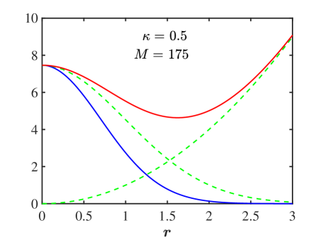
Figure 1: The density $\rho(r)$ (in blue) and confining potential $V(r)$ (in red) as a function of $r$ for the case when $\kappa=1/2$ and $M=175$ (see Table 1). The dotted green lines are plots of $V_{1}(r)$ and $V_{2}(r)$ for this case.

3 Lagrangian dynamics in two spatial dimensions

The Dirac action [17, 18] that upon variation leads to the NLSE of Eq. (2.1) for any potential $V(x,y)$ is given by

$$\Gamma[\psi,\psi^{\ast}] = \!\int\!\,\mathrm{d}t\,L[\psi,\psi^{\ast}]=\!\int\!\,\mathrm{d}t\,\{\,T[\psi,\psi^{\ast}]-H[\psi,\psi^{\ast}]\,\}\>,$$ (3.1)

$$T[\psi,\psi^{\ast}] = \int_{-\infty}^{+\infty}\,\mathrm{d}^{2}x\,\Bigl{[}\,\frac{\rmi}{2}\bigl{(}\psi^{\ast}(\partial_{t}\psi)-(\partial_{t}\psi^{\ast})\psi\,\bigr{)}\Bigr{]}\>,$$ (3.2)

$$H[\psi,\psi^{\ast}] = \int_{-\infty}^{+\infty}\,\mathrm{d}^{2}x\,\Bigl{[}\,\,|\nabla\psi|^{2}-\frac{g}{\kappa+1}\,(\psi^{\ast}\psi)^{\kappa+1}+V\,|\psi|^{2}\,\Bigr{]}\>.$$ (3.3)

Here $\,\mathrm{d}^{2}x\,=\,\mathrm{d}x\,\,\mathrm{d}y\,$. For spherically symmetric wavefunctions, the kinetic part of $H$ can be written in spherical coordinates as

$$K[\psi,\psi^{\ast}]=2\pi\int_{0}^{\infty}r\,\mathrm{d}r\,\Big{|}\frac{\partial\psi}{\partial r}\Big{|}^{2}=\int_{-\infty}^{\infty}\,\mathrm{d}x\,\int_{-\infty}^{\infty}\,\mathrm{d}y\,\Bigl{[}\,\Big{|}\frac{\partial\psi}{\partial x}\Big{|}^{2}+\Big{|}\frac{\partial\psi}{\partial y}\Big{|}^{2}\,\Bigr{]}\>.$$ (3.4)

3.1 Conserved quantities

From the equation of motion [cf. Eq. (2.1)], one finds that the $L^{2}$ norm of the wavefunction, called the mass $M$ hereafter, is conserved:

$$M=\!\int\!\,\mathrm{d}^{2}x\,|\psi(x,y,t)|^{2},$$ (3.5)

and for the exact solution of Eq. (2.2), the conserved mass reduces into

$$M=2\pi A_{0}^{2}\int_{0}^{\infty}\!\!\!r\,\rme^{-r^{2}/G_{0}}\,\mathrm{d}r\,=\pi\,G_{0}\,A_{0}^{2}\>,\quad A_{0}=\sqrt{\frac{M}{\pi G_{0}}}\>.$$ (3.6)

While studying the stability of the pertinent Gaussian waveforms, we will keep the mass of the initial condition unchanged (over time $t$), although its initial width will be of the form of $G(0)=G_{0}/\beta=G_{0}+\delta G_{0}$ (here, we adopt the notation $G(0)\doteq G(t=0)$). The initial height of the Gaussian for the perturbed solution is then given by:

$$A(0)=\sqrt{\frac{M}{\pi G(0)}}\>.$$ (3.7)

The (total) energy given by Eq. (3.3) is also conserved, and for the exact solution, it is explicitly given by:

$$\frac{E}{M}=\frac{2}{G_{0}}+\frac{g\,\kappa}{(\kappa+1)^{2}}\,\Bigl{(}\frac{M}{\pi\,G_{0}}\Bigr{)}^{\kappa}\>.$$ (3.8)

4 Derrick’s theorem

4.1 Width stability

First, we would like to see if the exact solution is stable to changes in the width while keeping the mass fixed. This is the criterion for stability due to Derrick [15]. It should be noted in passing that for $d=2$ and in the absence of the external potential, the solutions are unstable to changes in the width when $\kappa>1$. To that end, we set $r^{2}\rightarrow\beta\,r^{2}$ (with $\beta$ being the rescaling parameter), and take the stretched wavefunction as

$$\tilde{\psi}(r,t)=\tilde{A}\,\rme^{-\beta\,r^{2}/(2G_{0})-\rmi\,\varphi(t)}\>,$$ (4.1)

and examine what this transformation does to the Hamiltonian (3.3). Keeping the mass fixed, we arrive at

$$\tilde{A}^{2}=\frac{\beta M}{\pi G_{0}}=\beta\,A_{0}^{2}\>,$$ (4.2)

and thus, the density for the streched solution is given by:

$$\tilde{\rho}(r)=|\tilde{\psi}(r,t)|^{2}=\frac{\beta M}{\pi G_{0}}\rme^{-\beta\,r^{2}/G_{0}}\>.$$ (4.3)

To compare with previous work on blowup in the NLSE [16], we will eventually set $G_{0}=g=1$. We have that this solution contributes to the various components of the energy as follows:

$$H_{1} = 2\pi\int_{0}^{\infty}r\,\mathrm{d}r\,\Bigl{|}\frac{\partial\psi}{\partial r}\Bigr{|}^{2}=\frac{M\beta}{G_{0}}\>,$$ (4.4)

$$H_{2} = -\frac{g}{\kappa+1}\,2\pi\int_{0}^{\infty}r\,\mathrm{d}r\,\tilde{\rho}^{\kappa+1}(r)=-\frac{g\,M}{(\kappa+1)^{2}}\,\Bigl{[}\frac{\beta M}{\pi\,G_{0}}\Bigr{]}^{\kappa}\>,$$ (4.5)

$$H_{3} = 2\pi\int_{0}^{\infty}r\,\mathrm{d}r\,\tilde{\rho}(r)\,V_{1}(r)$$ (4.6)

$$= g\,\beta\Bigl{(}\frac{M}{\pi G_{0}}\Bigr{)}^{\kappa+1}\,2\pi\int_{0}^{\infty}r\,\mathrm{d}r\,e^{-(\kappa+\beta)\,r^{2}/G_{0}}=\frac{g\,\beta\,M}{\beta+\kappa}\,\Bigl{[}\frac{M}{\pi\,G_{0}}\Bigr{]}^{\kappa}\>,$$

$$H_{4} = 2\pi\int_{0}^{\infty}r\,\mathrm{d}r\,\tilde{\rho}(r)\,V_{2}(r)$$ (4.7)

$$= \frac{\beta M}{\pi G_{0}}\,\frac{2\pi}{G_{0}^{2}}\int_{0}^{\infty}r^{3}\,\mathrm{d}r\,\rme^{-\beta\,r^{2}/G_{0}}=\frac{M}{\beta\,G_{0}}\>.$$

The Hamiltonian denoted by $H_{\mathrm{w}}$ in this case, is then given by

$$\frac{H_{\mathrm{w}}(\beta)}{M}=\frac{1}{G_{0}}\,\Bigl{[}\,\beta+\frac{1}{\beta}\,\Bigr{]}-\frac{g}{(\kappa+1)^{2}}\,\Bigl{[}\frac{\beta M}{\pi\,G_{0}}\Bigr{]}^{\kappa}+\frac{g\,\beta}{\beta+\kappa}\,\Bigl{[}\frac{M}{\pi\,G_{0}}\Bigr{]}^{\kappa}\>.$$ (4.8)

Taking the first derivative of $H_{\mathrm{w}}$ with respect to $\beta$ we obtain

$$\frac{1}{M}\frac{\partial H_{\mathrm{w}}(\beta)}{\partial\beta}=\frac{1}{G_{0}}\,\Bigl{[}\,1-\frac{1}{\beta^{2}}\,\Bigr{]}+g\,\Big{[}\,\frac{\kappa}{(\beta+\kappa)^{2}}-\frac{\kappa\,\beta^{\kappa-1}}{(\kappa+1)^{2}}\,\Big{]}\,\Bigl{[}\frac{M}{\pi\,G_{0}}\Bigr{]}^{\kappa}\>.$$ (4.9)

From Eq. (4.9), we see that $\partial H/\partial\beta|_{\beta=1}=0$, therefore the solution we found is a stationary point of the stretched Hamiltonian. Taking the second derivative of $H_{\mathrm{w}}$ with respect to $\beta$, evaluating it at $\beta=1$ and dividing by the mass we obtain

$$\frac{1}{M}\,\frac{\partial^{2}H_{\mathrm{w}}(\beta)}{\partial\beta^{2}}\Big{|}_{\beta=1}=\frac{2}{G_{0}}-g\,\frac{\kappa(\kappa^{2}+1)}{(\kappa+1)^{3}}\Bigl{[}\,\frac{M}{\pi G_{0}}\,\Bigr{]}^{\kappa}\>.$$ (4.10)

Derrick’s theorem predicts that the soliton is stable to width perturbations (by keeping $M$ fixed), if Eq. (4.10) is positive, or

$$M<M_{\mathrm{w}}(\kappa)=\pi G_{0}\,\Bigl{[}\,\frac{2}{gG_{0}}\,\frac{(\kappa+1)^{3}}{\kappa(\kappa^{2}+1)}\,\Bigr{]}^{1/\kappa}\>,$$ (4.11)

which reduces into

$$M<M_{\mathrm{w}}(\kappa)=\pi\,\Bigl{[}\,\frac{2\,(\kappa+1)^{3}}{\kappa\,(\kappa^{2}+1)}\,\Bigr{]}^{1/\kappa}\>,$$ (4.12)

upon setting $G_{0}=1$ (and $g=1$ as before). The behavior of critical mass $M^{\ast}_{\mathrm{w}}(\kappa)$ is shown in red in Fig. 2. Since $M^{\ast}\rightarrow\pi$ as $\kappa\rightarrow\infty$, the exact solution is stable for all values of $\kappa$ provided that $M<\pi$. In terms of the amplitude $\tilde{A}$ we have instead stability if

$$\tilde{A}<\tilde{A}_{\mathrm{w}}(\kappa)=\Bigl{[}\,\frac{2\,(\kappa+1)^{3}}{\kappa\,(\kappa^{2}+1)}\Bigr{]}^{1/(2\kappa)}\>.$$ (4.13)

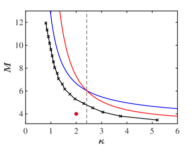
(a) $M_{\mathrm{w}}$ (red), $M_{\mathrm{t}}$ (blue), and numerical BdG analysis (black).

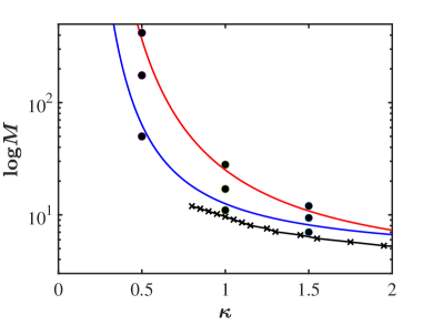
(b) Data points for 4CC simulations (see table 1).

Figure 2: The critical width mass $M_{\mathrm{w}}$ (red), critical translational mass $M_{\mathrm{t}}$ (blue), and BdG analysis (black) as a function of $\kappa$ (see also, Fig. 8 in Section 7). The red data point in panel (a) corresponds to the simulation shown in Fig. 7. The dashed vertical line is at the intersection point $\kappa=1+\sqrt{2}$.

4.2 Translational stability

Similar to Derrick’s theorem for width stability, we can ask what happens when we shift the position of the solution away from the origin. For simplicity let us consider $x\rightarrow x+a$ and ask whether the energy of the solution goes up or down. We will find that $x=0$ is an extremum of the potential, and that there is a critical mass $M_{\mathrm{t}}$ which is dependent on $\kappa$, above which the exact solution becomes a maximum of $H(a,\kappa)$. So we now consider the shifted wavefunction:

$$\tilde{\psi}(x,y,t)=A_{0}\,\rme^{-[\,(x-a)^{2}+y^{2}\,]/(2\,G_{0})-\rmi\,\varphi(t)}\>,\quad A_{0}^{2}=\frac{M}{\pi G_{0}}\>.$$ (4.14)

This shift in the position does not effect $H_{1}$ and $H_{2}$, and thus we get:

$$H_{1} = \frac{M}{G_{0}}\>,$$ (4.15)

$$H_{2} = -\frac{g\,M}{(\kappa+1)^{2}}\,\Bigl{[}\frac{M}{\pi\,G_{0}}\Bigr{]}^{\kappa}\>,$$ (4.16)

$$H_{3} = \int_{-\infty}^{\infty}\,\mathrm{d}x\,\int_{-\infty}^{\infty}\,\mathrm{d}y\,|\,\tilde{\psi}[x,y,Q(t)]\,|^{2}\,V_{1}(x,y)$$

$$= g\,\Bigl{(}\frac{M}{\pi G_{0}}\Bigr{)}^{\kappa+1}\int_{-\infty}^{\infty}\,\mathrm{d}x\,\int_{-\infty}^{\infty}\,\mathrm{d}y\,\,\rme^{-[(x-a)^{2}+y^{2}+\kappa(x^{2}+y^{2})]/G_{0}}$$

$$= \frac{g\,M}{\kappa+1}\,\Bigl{[}\frac{M}{\pi\,G_{0}}\Bigr{]}^{\kappa}\,\rme^{-\kappa\,a^{2}/[\,(\kappa+1)\,G_{0}\,]}\>,$$

$$H_{4} = \int_{-\infty}^{\infty}\,\mathrm{d}x\,\int_{-\infty}^{\infty}\,\mathrm{d}y\,|\,\tilde{\psi}[x,y,Q(t)]\,|^{2}\,V_{2}(x,y)$$ (4.18)

$$= \frac{M}{\pi G_{0}^{3}}\int_{-\infty}^{\infty}\,\mathrm{d}x\,\int_{-\infty}^{\infty}\,\mathrm{d}y\,\,(x^{2}+y^{2})\,\rme^{-[\,(x-a)^{2}+y^{2}\,]/G_{0}}=\frac{M}{G_{0}^{2}}\,(\,G_{0}+a^{2}\,)\>.$$

This way, the displaced Hamiltonian denoted by $H_{\mathrm{t}}(a)$ reads

$$\frac{H_{\mathrm{t}}(a)}{M} = \frac{1}{G_{0}}+\frac{g}{(\kappa+1)^{2}}\,\Bigl{[}\frac{M}{\pi\,G_{0}}\Bigr{]}^{\kappa}$$

$$\hskip 10.00002pt+\frac{g}{\kappa+1}\,\Bigl{[}\frac{M}{\pi\,G_{0}}\Bigr{]}^{\kappa}\,\rme^{-\kappa\,a^{2}/[\,(\kappa+1)\,G_{0}\,]}+\frac{1}{G_{0}^{2}}\,(\,G_{0}+a^{2}\,)\>.$$

The first derivative of this expression with respect to $a$ is

$$\frac{\partial H_{\mathrm{t}}(a)}{\partial a}=-\frac{2g\,\kappa\,a}{(\kappa+1)^{2}}\,\Bigl{[}\frac{M}{\pi\,G_{0}}\Bigr{]}^{\kappa}\,\rme^{-\kappa\,a^{2}/[\,(\kappa+1)\,G_{0}\,]}+\frac{2\,a}{G_{0}^{2}}\>,$$ (4.20)

and gives zero at $a=0$, showing that the exact solution is indeed an extremum of the energy. The second derivative at $a=0$ yields

$$\frac{\partial^{2}H_{\mathrm{t}}(a)}{\partial a^{2}}\Big{|}_{a=0}=\frac{2}{G_{0}^{2}}-\frac{2g\,\kappa}{(\kappa+1)^{2}}\,\Bigl{[}\frac{M}{\pi\,G_{0}}\Bigr{]}^{\kappa}\>,$$ (4.21)

and stability with respect to translations $a$ (again, while keeping $M$ fixed), requires that

$$M<M_{\mathrm{t}}(\kappa)=\pi G_{0}\Bigl{[}\frac{(\kappa+1)^{2}}{g\,G_{0}^{2}\,\kappa}\Bigr{]}^{1/\kappa}\>,$$ (4.22)

which reduces into

$$M<M_{\mathrm{t}}(\kappa)=\pi\Bigl{[}\frac{(\kappa+1)^{2}}{\kappa}\Bigr{]}^{1/\kappa}\>,$$ (4.23)

upon setting $G_{0}=1$ (and $g=1$ again). We see that $M_{\mathrm{t}}^{\ast}(\kappa)>\pi$, so that as long as $M<\pi$ there is no translational instability. The curve for $M_{\mathrm{t}}^{\ast}(\kappa)$ is shown in red in Fig. 2 and compared to the critical mass for the width instability. By comparing (4.23) with (4.12), we find that there is a crossover effect at $\kappa=1+\sqrt{2}$. Below $\kappa=1+\sqrt{2}$, the translational instability occurs first. Above this value the width instability occurs first. It is worth pointing out again that when $M<\pi$, there is neither translational nor width instability regardless of the value of $\kappa$.

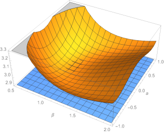
(a)  Stable case: $M=(4/5)\,M_{\mathrm{t}}$.

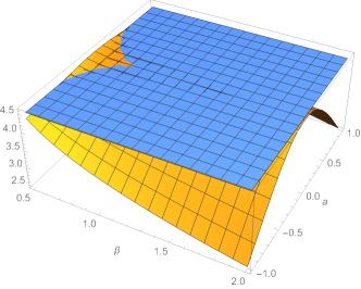
(b)  Unstable case: $M=(11/10)\,M_{\mathrm{w}}$.

Figure 3: Plots of the energy landscapes $E(a,\beta)/M$ (yellow) and the exact energy $E(0,1)/M$ (blue) for $\kappa=1/2$ for two values of $M$.

4.3 The potential energy landscape

Stability for both translations and stretches can be studied through the wavefunction of the form of

$$\tilde{\psi}(x,y,t)=A\,\rme^{-\beta[\,(x-a)^{2}+y^{2}\,]/2-\rmi\,\varphi(t)}\>,\quad A^{2}=\frac{\beta\,M}{\pi}=\beta\,A_{0}^{2}\>,$$ (4.24)

whose total energy is given by

$$\frac{E(a,\beta)}{M}=a^{2}+\beta+\frac{1}{\beta}-\Bigl{[}\,\frac{M}{\pi}\Bigr{]}^{\kappa}\,\Bigl{[}\,\frac{\beta^{\kappa}}{(\kappa+1)^{2}}-\frac{\beta}{\kappa+\beta}\,\rme^{-\kappa\,\beta\,a^{2}/(\kappa+\beta)}\,\Bigr{]}\>.$$ (4.25)

There are two critical masses for translational and width instabilities, given respectively by

$$M_{\mathrm{t}} = \pi\,[(\kappa+1)^{2}/\kappa]^{1/\kappa}\>,$$ (4.26)

$$M_{\mathrm{w}} = \pi\,[\,2\,(\kappa+1)^{3}/(\kappa(\kappa^{2}+1)\,)\,]^{1/\kappa}\>.$$ (4.27)

For the exact energy, $\alpha=0$ and $\beta=1$,

$$\frac{E(0,1)}{M}=2+\frac{\kappa}{(\kappa+1)^{2}}\,\Bigl{[}\,\frac{M}{\pi}\Bigr{]}^{\kappa}\>,$$ (4.28)

which is in agreement with Eq. (3.8). To show how intricate the energy landscape can be, we display two cases for $\kappa=1/2$ in Fig. 3. If we are in the regime where the mass is less than both critical masses, then by choosing $M=(4/5)\,M_{\mathrm{t}}$, we get the results shown in Fig. 3(a). If instead we choose $M=(11/10)\,M_{\mathrm{w}}$, then we are in the unstable regime as shown in Fig. 3(b) .

4.4 Derrick’s theorem in the absence of a potential

In contrast, when $V(\mathbf{r})\equiv 0$, Derrick’s theorem for width stability does not provide one with a critical mass. Instead, from Eq. (4.8) (and for $g=G_{0}=1$), we directly obtain

$$\frac{H(\beta)}{M}=\beta-\frac{1}{(\kappa+1)^{2}}\,\Bigl{[}\frac{\beta M}{\pi}\Bigr{]}^{\kappa}\>,$$ (4.29)

whose first derivative yields

$$\frac{1}{M}\frac{\partial H}{\partial\beta}=1-\frac{\kappa\,\beta^{\kappa-1}}{(\kappa+1)^{2}}\,\Bigl{[}\frac{M}{\pi}\Bigr{]}^{\kappa}\>.$$ (4.30)

Choosing $M=M_{1}$, where

$$M_{1}=\pi\,\Bigl{[}\frac{(\kappa+1)^{2}}{\kappa}\Bigr{]}^{1/\kappa}\>,$$ (4.31)

then Eq. (4.30) vanishes at $\beta=1$ showing that this is an extremum. The condition for this to be a minimum is that

$$\frac{1}{M}\frac{\partial^{2}H}{\partial\beta^{2}}\Big{|}_{\beta=1}=-\frac{\kappa\,(\kappa-1)}{(\kappa+1)^{2}}\Bigl{[}\frac{M_{1}}{\pi}\Bigr{]}^{\kappa}=1-\kappa>0\>,$$ (4.32)

so that for the 2D NLSE, stability is guaranteed as long as $\kappa<1$. In arbitrary dimensions $d$ a similar calculation yields stability for $\kappa d<2$.

5 Collective coordinate method

The collective coordinate (CC) method uses a variational ansatz to solve for the dynamics from the action given in Eq. (3.1) for the NLSE in an external potential. In this paper we will employ a four CC ansatz so that we can explore the response of the solution when we perturb the initial wavefunction both in the width as well as in the position. The method we use here is similar to the method introduced in a previous paper, and authored by some of the current authors [16]. We restrict our calculation here to 4CCs, which allows us to recover the results of Derrick’s theorem. However, by comparing these with numerical results of the NLSE in the unstable regime, we find that translations in the $y$ direction, which were not included here, get excited. Also, once instabilities manifest themselves, the shape of the wavefunction starts deviating from our assumed Gaussian shape.

5.1 Two collective coordinate (2CC) ansatz

If we are just interested in the dynamics of the width of self-similar solutions, we can assume that the wavefunction can be parametrized by two CCs, and thus choose

$$\tilde{\psi}[r,Q(t)] = \tilde{A}(t)\,\rme^{-r^{2}/[2G(t)]+\rmi\,\Lambda(t)\,r^{2}-\rmi\,\varphi(t)}\>,$$

$$M = \int\,\mathrm{d}^{2}x\,|\tilde{\psi}[r,Q(t)]|^{2}=\pi\,G(t)\,\tilde{A}^{2}(t)\>,$$

$$Q(t) = \{G(t),\Lambda(t)\}\>.$$ (5.1)

Here $\tilde{A}(t)$ is fixed by $M$ and $G(t)$ so $\varphi(t)$ is irrelevant to the dynamics. This Gaussian ansatz (5.1) agrees with the results of Perez-Garcia [19], who showed that if one has a self-similar solution of the NLSE of the form

$$\tilde{\psi}[r,w(t),\phi(r,t)]=\tilde{A}(t)\,\rho\Bigl{[}\frac{r}{w(t)}\Bigr{]}\,\rme^{\rmi\,\phi(r,t)}\>,$$ (5.2)

then the phase is fixed to be quadratic and of the form

$$\phi(r,t)=\frac{\dot{w}}{2w}\,r^{2}\>.$$ (5.3)

From Lagrange’s equations for the collective coordinates (see below) we will find

$$\Lambda=\dot{G}/(8G)\>.$$ (5.4)

5.2 Four collective coordinate (4CC) ansatz

To compare with our energy landscape static calculation above, it is sufficient to consider the response of the wavefunction to translations in one spatial direction, which we will choose to be the $x$ direction. Indeed, we can study the response of the wavefunction to small perturbations in width and position through a suitable 4CC ansatz in a variational approach by replacing

$$x^{2}+y^{2}\rightarrow\bar{x}^{2}(t)+y^{2}\>,\quad\bar{x}(t)=x-q_{x}(t)\>.$$ (5.5)

The conjugate coordinate to $q_{x}(t)$ is the momentum $p_{x}(t)$ as a collective coordinate. For simplicity, we will suppress the subindex $x$ on $q,p$, and choose for our 4CC variational wavefunction:

$$\tilde{\psi}[x,y,Q(t)] = A(t)\,\rme^{\phi(x,y,t)}\>,\quad M=\pi\,G(t)\,A^{2}(t)=\pi\,G_{0}\,A_{0}^{2}\>,$$

$$\phi[x,y,Q(t)] = -\frac{\bar{x}^{2}(t)+y^{2}}{2G(t)}+\rmi\,[\,p(t)\,\bar{x}(t)+\Lambda(t)\,(\bar{x}^{2}(t)+y^{2})+\varphi(t)\,]\>.$$ (5.6)

Here again $A(t)$ is fixed by $M$ and $G(t)$ and is not a dynamic variable. This means that $\varphi(t)$ is not dynamic either, and we ignore it in the following, so then the four generalized coordinates are: $Q(t)=\{\,q(t),p(t),G(t),\Lambda(t)\,\}$. The $x$-displacement $q(t)$ and width $G(t)$ are then given by the integrals:

$$q(t) = \frac{1}{M}\int_{-\infty}^{\infty}\,\mathrm{d}x\,\int_{-\infty}^{\infty}\,\mathrm{d}y\,|\,\tilde{\psi}[x,y,Q(t)]\,|^{2}\,x\>,$$ (5.7)

$$G(t) = \frac{1}{M}\int_{-\infty}^{\infty}\,\mathrm{d}x\,\int_{-\infty}^{\infty}\,\mathrm{d}y\,|\,\tilde{\psi}[x,y,Q(t)]\,|^{2}\,[\,\bar{x}^{2}(t)+y^{2}\,]\>.$$ (5.8)

Using Eqs. (5.7) and (5.8), it is easy to extract the variational parameters from simulations by calculating the first two moments of the density. When we insert the variational wavefunction into the complete action of Eq. (3.1) and integrate over the spatial degrees of freedom, we get an effective action for the variational parameters. In this process, we keep the parameters of the potential fixed by the exact solution. Writing the external potential in terms of the conserved mass $M$ with $V(r)=V_{1}(r)+V_{2}(r)$, from Eq. (2.3), we have

$$V_{1}(r)=g\,\Bigl{(}\frac{M}{\pi G_{0}}\Bigr{)}^{\kappa}\rme^{-\kappa\,r^{2}/G_{0}}\>,\quad V_{2}(r)=\Bigl{(}\frac{r}{G_{0}}\Bigr{)}^{2}\>.$$ (5.9)

The action then takes the form

$$\Gamma[Q]=\!\int\!\,\mathrm{d}t\,L[\,Q,\dot{Q}]\>,$$ (5.10)

where the Lagrangian is given by

$$L[\,Q,\dot{Q}]=M\,[\,p(t)\,\dot{q}(t)+\Lambda(t)\,\dot{G}(t)\,]-H[\,Q\,]\>.$$ (5.11)

The Hamiltonian is a sum of four terms

$$H(Q)=H_{1}(Q)+H_{2}(Q)+H_{3}(Q)+H_{4}(Q)\>,$$ (5.12)

where

$$H_{1}(Q) = \int_{-\infty}^{\infty}\,\mathrm{d}x\,\int_{-\infty}^{\infty}\,\mathrm{d}y\,\Bigl{[}\,|\partial_{x}\tilde{\psi}(x,y)|^{2}+|\partial_{y}\tilde{\psi}(x,y)|^{2}\,\Bigr{]}\>,$$ (5.13)

$$= \int_{-\infty}^{\infty}\,\mathrm{d}x\,\int_{-\infty}^{\infty}\,\mathrm{d}y\,\Bigl{[}\,|\bar{x}/G+\rmi p+2\rmi\Lambda\bar{x}|^{2}+|y/G+2\rmi\Lambda y|^{2}\,\Bigr{]}\,|\tilde{\psi}|^{2}\>,$$

$$= \frac{M}{\pi G}\int_{-\infty}^{\infty}\,\mathrm{d}x\,\int_{-\infty}^{\infty}\,\mathrm{d}y\,\,\rme^{-(\bar{x}^{2}+y^{2})/G}\,\Bigl{[}\,p^{2}+4\,\Lambda^{2}(\,\bar{x}^{2}+y^{2})+\frac{\bar{x}^{2}+y^{2}}{G^{2}}\,\Bigr{]}$$

$$= M\,(p^{2}+4\,G\,\Lambda^{2}+1/G)\>,$$

$$H_{2}(Q) = -\frac{g}{\kappa+1}\int_{-\infty}^{\infty}\,\mathrm{d}x\,\int_{-\infty}^{\infty}\,\mathrm{d}y\,\,|\tilde{\psi}(x,y)|^{2\kappa+2}$$ (5.14)

$$= -\frac{g}{\kappa+1}\,\Bigl{[}\,\frac{M}{\pi G}\Bigr{]}^{\kappa+1}\int_{-\infty}^{\infty}\,\mathrm{d}x\,\int_{-\infty}^{\infty}\,\mathrm{d}y\,\,\rme^{-(\kappa+1)(\bar{x}^{2}+y^{2})/G}$$

$$= -\frac{gM}{(\kappa+1)^{2}}\,\Bigl{[}\,\frac{M}{\pi G}\Bigr{]}^{\kappa}\>,$$

$$H_{3}(Q) = \int_{-\infty}^{\infty}\,\mathrm{d}x\,\int_{-\infty}^{\infty}\,\mathrm{d}y\,\,|\tilde{\psi}(x,y)|^{2}\,V_{1}(x,y)$$ (5.15)

$$= g\,\Bigl{[}\,\frac{M}{\pi G_{0}}\Bigr{]}^{\kappa}\,\Bigl{[}\,\frac{M}{\pi G}\Bigr{]}\,\int_{-\infty}^{\infty}\,\mathrm{d}x\,\int_{-\infty}^{\infty}\,\mathrm{d}y\,\,\rme^{-\kappa(x^{2}+y^{2})/G_{0}-(\bar{x}^{2}+y^{2})/G}$$

$$= g\,\frac{M\,G_{0}}{G\kappa+G_{0}}\,\Bigl{[}\,\frac{M}{\pi G_{0}}\Bigr{]}^{\kappa}\,\rme^{-\kappa\,q^{2}/(\kappa G+G_{0})}\>,$$

$$H_{4}(Q) = \int_{-\infty}^{\infty}\,\mathrm{d}x\,\int_{-\infty}^{\infty}\,\mathrm{d}y\,\,|\tilde{\psi}(x,y)|^{2}\,V_{2}(x,y)$$ (5.16)

$$= \frac{1}{G_{0}^{2}}\,\Bigl{[}\,\frac{M}{\pi G}\Bigr{]}\int_{-\infty}^{\infty}\,\mathrm{d}x\,\int_{-\infty}^{\infty}\,\mathrm{d}y\,\,(\,x^{2}+y^{2}\,)\,\rme^{-(\bar{x}^{2}+y^{2})/G}$$

$$= \frac{M}{G_{0}^{2}}\,(\,G+q^{2}\,)\>.$$

Adding these terms, the total Hamiltonian is given by

$$\frac{H(Q)}{M} = p^{2}+\frac{q^{2}}{G_{0}^{2}}+\frac{G}{G_{0}^{2}}+\frac{1}{G}+4\,G\,\Lambda^{2}-\frac{g}{(\kappa+1)^{2}}\,\Bigl{[}\,\frac{M}{\pi G}\Bigr{]}^{\kappa}$$ (5.17)

$$\hskip 20.00003pt+\frac{g\,G_{0}}{G\kappa+G_{0}}\,\Bigl{[}\,\frac{M}{\pi G_{0}}\Bigr{]}^{\kappa}\,\rme^{-\kappa\,q^{2}/(\kappa G+G_{0})}\>.$$

Note that Eq. (5.17) agrees with Eq. (3.8) when $q=p=\Lambda=0$. The Lagrangian for the 4CC ansatz is then given by:

$$\frac{L[\,Q,\dot{Q}\,]}{M} = p\,\dot{q}+\Lambda\,\dot{G}-p^{2}-\frac{q^{2}}{G_{0}^{2}}-\frac{G}{G_{0}^{2}}-\frac{1}{G}-4\,G\,\Lambda^{2}+\frac{g}{(\kappa+1)^{2}}\,\Bigl{[}\,\frac{M}{\pi G}\Bigr{]}^{\kappa}$$ (5.18)

$$\hskip 20.00003pt-\frac{g\,G_{0}}{G\kappa+G_{0}}\,\Bigl{[}\,\frac{M}{\pi G_{0}}\Bigr{]}^{\kappa}\,\rme^{-\kappa\,q^{2}/(\kappa G+G_{0})}\>.$$

From Eq. (5.18), the equations of motion are

$$\dot{q} = 2\,p\>,$$ (5.19)

$$\dot{p} = -\frac{2\,q}{G_{0}^{2}}+\frac{2g\,\kappa\,G_{0}\,q}{(G\kappa+G_{0})^{2}}\,\Bigl{[}\,\frac{M}{\pi G_{0}}\Bigr{]}^{\kappa}\,\rme^{-\kappa\,q^{2}/(G\kappa+G_{0})}\>,$$ (5.20)

$$\dot{G} = 8\,G\,\Lambda\>,$$ (5.21)

$$\dot{\Lambda} = -4\,\Lambda^{2}-\frac{1}{G_{0}^{2}}+\frac{1}{G^{2}}-\frac{g\,\kappa}{(\kappa+1)^{2}\,G}\,\Bigl{[}\,\frac{M}{\pi G}\Bigr{]}^{\kappa}$$ (5.22)

$$\hskip 10.00002pt+\frac{g\,G_{0}\,\kappa}{(G\kappa+G_{0})^{2}}\,\Bigl{[}\,1-\frac{\kappa\,q^{2}}{G\kappa+G_{0}}\,\Bigr{]}\,\Bigl{[}\,\frac{M}{\pi G_{0}}\Bigr{]}^{\kappa}\,\rme^{-\kappa\,q^{2}/(G\kappa+G_{0})}\>.$$

5.3 Blowup time

Using the equation of motion for $\dot{G}$, and setting $G_{0}=1$, we can rewrite the energy as

$$\frac{E(Q)}{M} = p^{2}+q^{2}+\frac{\dot{G}^{2}}{16\,G}+G+\frac{1}{G}-\frac{g}{(\kappa+1)^{2}}\,\Bigl{[}\,\frac{M}{\pi\,G}\Bigr{]}^{\kappa}$$ (5.23)

$$\hskip 10.00002pt+\frac{g}{G\kappa+1}\,\Bigl{[}\,\frac{M}{\pi}\Bigr{]}^{\kappa}\,\rme^{-\kappa\,q^{2}/(\kappa G+1)}\>.$$

We will see below from our simulations that one can have blowup ($G\rightarrow 0$), as long as $\kappa\geq 2$ and $M>M^{\ast}$. The energy is conserved, and constrains the range of $G$ and $q$. The initial energy of the perturbed solution is given by Eq. (5.23) with $q=q(t=0),p=p(t=0),G=G(t=0),\dot{G}=\dot{G}(t=0)$, which for our simulations will be close to the energy of the exact solution $E=E_{0}$, and is given by Eq. (3.8), or

$$\frac{E_{0}}{M}=2+\frac{g\,\kappa}{(\kappa+1)^{2}}\,\Bigl{[}\frac{M}{\pi}\Bigr{]}^{\kappa}\>.$$ (5.24)

When $G\rightarrow 0$, from the leading terms (that must cancel), we obtain

$$\dot{G}=-\sqrt{\frac{16\,G(t)}{(\kappa+1)^{2}}\,\Bigl{[}\frac{M}{\pi\,G(t)}\Bigr{]}^{\kappa}}=-\frac{4M^{\kappa/2}}{\pi^{\kappa/2}(\kappa+1)}G(t)^{(1-\kappa)/2}\>,$$ (5.25)

which can be integrated, thus yielding (near the blowup time $t^{\ast}$ with $t<t^{\ast}$)

$$G(t)=\frac{4M^{\kappa/2}}{\pi^{\kappa/2}(\kappa+1)^{2}}\,(t-t^{\ast})^{2/(\kappa+1)}\>.$$ (5.26)

References to blowup times can be found in [10, 20].

5.4 Small amplitude approximation for the 4CC dynamics

From Eqs. (5.19 - 5.22), we can obtain small oscillation equations by setting $G_{0}=1$, letting

$$q=\delta q\>,\quad p=\delta p\>,\quad G=1+\delta G\>,\quad\Lambda=\delta\Lambda\>,\quad\left(\delta q,\delta p,\delta G,\delta\Lambda\ll 1\right)\>,$$ (5.27)

and keeping only the linear terms. We obtain:

$$\delta\dot{q} = 2\,\delta p\>,$$ (5.28)

$$\delta\dot{p} = -2\,\Bigl{\{}\,1-\frac{g\kappa}{(\kappa+1)^{2}}\,\Bigl{[}\,\frac{M}{\pi}\Bigr{]}^{\kappa}\,\Bigr{\}}\,\delta q\>,$$ (5.29)

$$\delta\dot{G} = 8\,\delta\Lambda\>,$$ (5.30)

$$\delta\dot{\Lambda} = -\Bigl{\{}\,2-\frac{g\,\kappa(\kappa^{2}+1)}{(\kappa+1)^{3}}\,\Bigl{[}\,\frac{M}{\pi}\Bigr{]}^{\kappa}\,\Bigr{\}}\,\delta G\>.$$ (5.31)

We observe from the above that the $(\delta q,\delta p)$ dynamics decouple from the $(\delta G,\delta\Lambda)$ dynamics, and thus we find the small oscillations are governed by the equations

$$\delta\ddot{q}+\omega_{q}^{2}\,\delta q=0\>,\quad\delta\ddot{G}+\omega_{G}^{2}\,\delta G=0\>,$$ (5.32)

with

$$\omega_{q}^{2} = 4\,\Bigl{\{}\,1-\frac{g\,\kappa}{(\kappa+1)^{2}}\,\Bigl{[}\,\frac{M}{\pi}\Bigr{]}^{\kappa}\,\Bigr{\}}=4\,\Bigl{\{}\,1-\Bigl{[}\,\frac{M}{M_{\mathrm{t}}}\Bigr{]}^{\kappa}\,\Bigr{\}}\>,$$ (5.33)

$$\omega_{G}^{2} = 8\,\Bigl{\{}\,2-\frac{g\,\kappa\,(\kappa^{2}+1)}{(\kappa+1)^{3}}\,\Bigl{[}\,\frac{M}{\pi}\Bigr{]}^{\kappa}\,\Bigr{\}}=16\,\Bigl{\{}\,1-\Bigl{[}\,\frac{M}{M_{\mathrm{w}}}\Bigr{]}^{\kappa}\,\Bigr{\}}\>,$$ (5.34)

where $M_{\mathrm{t}}$ and $M_{\mathrm{w}}$ are given in Eqs. (4.26-4.27). For the $\delta q$ dynamics (translational) to be stable, we must have $M<M_{\mathrm{t}}$, and for the $\delta G$ dynamics (width) to be stable, we must have $M<M_{\mathrm{w}}$.

6 Typical evolutions in the 4CC approximation

Here we explore the behavior of the 4CC ansatz for $\kappa$ in the range $1/2\leq\kappa\leq 3/2$ which surrounds the critical value of $\kappa=1$ for blowup in the absence of a potential. We consider three cases, $\kappa=1/2$, $\kappa=1$, and $\kappa=3/2$. For these three cases we choose masses in three regimes:

1. $M<M_{\mathrm{t}},M_{\mathrm{w}}$  ,

2. $M_{\mathrm{t}}<M<M_{\mathrm{w}}$  ,

3. $M_{\mathrm{t}},M_{\mathrm{w}}<M$  .

For illustrative purposes for the 4CC simulations, we will take for the exact solution: $g=G_{0}=1$, and the initial values of $G(t=0)=0.99$, $\Lambda(t=0)=0$, $q(t=0)=0.01$, and $p(t=0)=0$. The values of $M$, initial values of $A_{0}$ and the energy $E(t=0)$ for the initial trial wavefunction of Eq. (5.6) are given in Table 1.

Table 1: Values of $\kappa$, mass ($M$), and energy ($E$) used in Section 6 and plotted in Figure 2(a). We use initial values of $G_{0}=0.99$, $\Lambda_{0}=0$, $q_{0}=0.01$, and $p_{0}=0$.

$\kappa$	case	$M$	$A_{0}$	$E_{0}$
$1/2$	(a)	50	4.0095	2.8866
	(b)	175	7.5011	3.6585
	(c)	419	11.6069	4.5662
$1$	(a)	11	1.8806	2.8754
	(b)	17	2.3379	3.3528
	(c)	28	3.0005	4.2280
$3/2$	(a)	7	1.5002	2.7983
	(b)	9.4	1.7385	3.2422
	(c)	12	1.9642	3.7916

6.1 $\kappa=1/2$

Case (a): Using the data of Table 1, the solutions for $q(t)$ and $G(t)$ never go unstable in the absence of an external potential. With an external potential we get the results shown in Fig. 4(a). The oscillation frequencies here match the prediction of the 4CC small amplitude approximation.

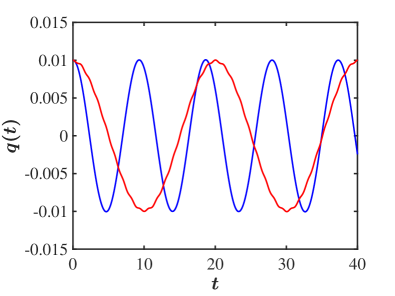
(a) $q(t)$ case a

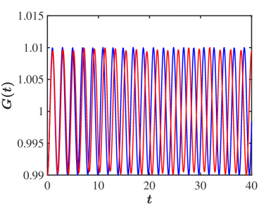
(b) $G(t)$ case a

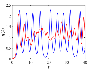
(c) $q(t)$ case b

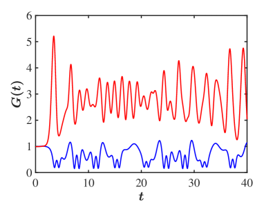
(d) $G(t)$ case b

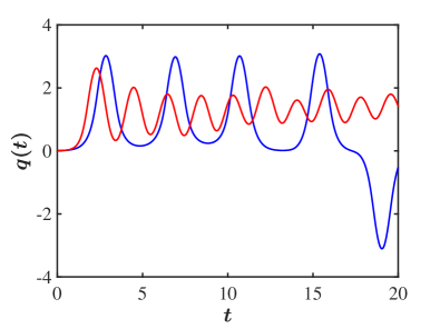
(e) $q(t)$ case c

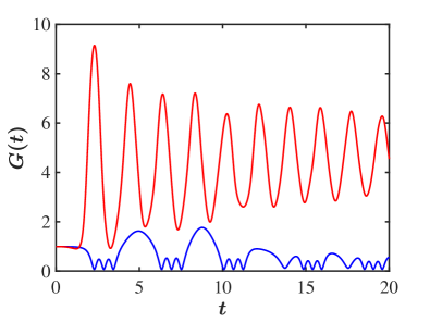
(f) $G(t)$ case c

Figure 4: Plots of $q(t)$ and $G(t)$ for the 4CC results (blue) and numerical NLSE results (red), for $\kappa=1/2$. See Table 1 for mass parameters.

Case (b): Here $q(t)$ tries to escape the potential well, and $G$ tries to go to zero (blowup) or infinity (collapse). However, energy conservation prevents both blowup and escape of the initial wavefunction, and we get the semi-oscillating behavior shown in Fig. 4(c).

Case (c): Similarly, blowup of $G(t)$ is stalled because of energy conservation. The $q(t)$ growth also stalls, and $q(t)$ switches from being greater than zero to being less than zero. This is seen in Fig. 4(e).

6.2 $\kappa=1$

Case (a): In this case, $\kappa=1$ is the critical value for blowup in the absence of a confining potential. Moreover, blowup occurs in this case when for the initial conditions $M\geq M_{\mathrm{w}}$ holds. The 4CC results of Fig. 5(a) show that $q(t)$ and $G(t)$ oscillate, and are in the small amplitude regime. The period for $G(t)$ from the small amplitude approximation is $T_{G}=2.118$ and the period for $q(t)$ is $T_{q}=9.934$.

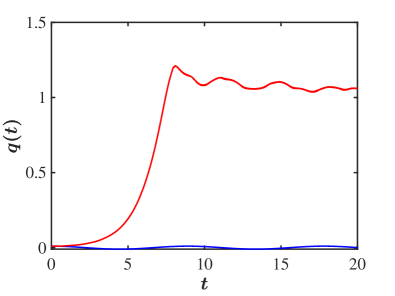
(a) $q(t)$ case a

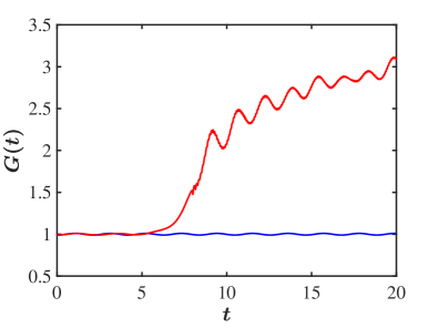
(b) $G(t)$ case a

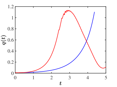
(c) $q(t)$ case b

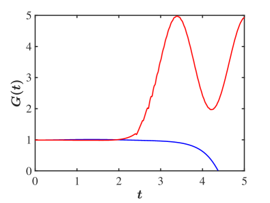
(d) $G(t)$ case b

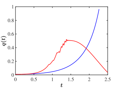
(e) $q(t)$ case c

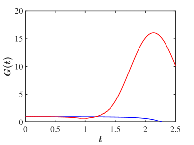
(f) $G(t)$ case c

Figure 5: Plots of $q(t)$ and $G(t)$ for the 4CC results (blue) and numerical NLSE results (red), for $\kappa=1$. See Table 1 for mass parameters.

Case (b): If we are in the in-between case, then after one oscillation of the $G(t)$ variable, the wavefunction blows up as a result of the $q(t)$ instability. This is seen in Fig. 5(c) for $G(t)$ and $q(t)$.

Case (c): When we are above the critical mass, the solution blows up much quicker. For this case, the blowup time is shortened to about $t_{f}=2.3$, which is seen in Fig. 5(e).

6.3 $\kappa=3/2$

Case (a): In the absence of a confining potential, when $\kappa=3/2$ we are always in a blowup regime. However with a confining potential, the 4CC results shown in Fig. 6(a) indicate that we are in a small amplitude regime. The two periods are predicted from the small amplitude approximation are $T_{q}=8.21$ and $T_{G}=2.35$, which agree quite well with simulations.

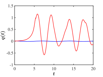
(a) $q(t)$ case a

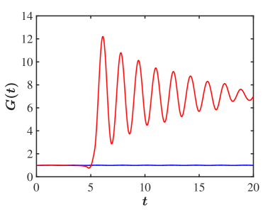
(b) $G(t)$ case a

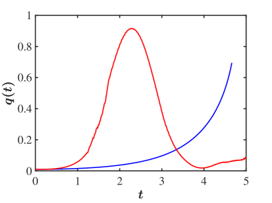
(c) $q(t)$ case b

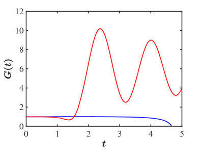
(d) $G(t)$ case b

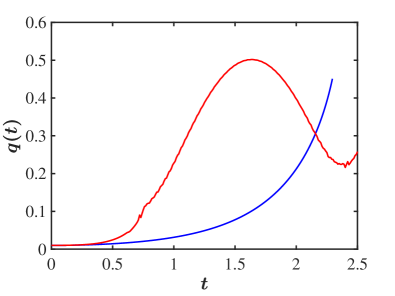
(e) $q(t)$ case c

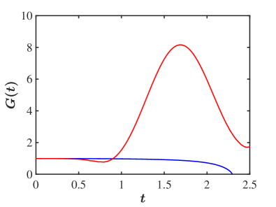
(f) $G(t)$ case c

Figure 6: Plots of $q(t)$ and $G(t)$ for the 4CC results (blue) and numerical NLSE results (red), for $\kappa=3/2$. See Table 1 for mass parameters.

Case (b): The results of the 4CC simulation for $G(t)$ and $q(t)$ are shown in Fig. 6(c), where we find that $q(t)$ is unstable but $G(t)$ is initially stable for one period and then the wavefunction blows up at $t\approx 4$ as a result of the translation instability.

Case (c): For this case, we see from Figs. 6(e) and 6(f) that both $q(t)$ and $G(t)$ blow up quicker, and the blowup happens at $t\approx 3.5$.

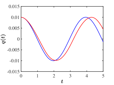
(a) $q(t)$ and $M=4.0$

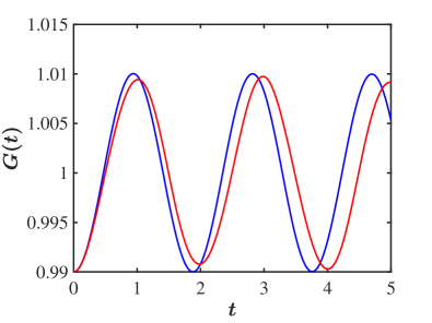
(b) $G(t)$ and $M=4.0$

Figure 7: Plots of $q(t)$ and $G(t)$ for the 4CC results (blue) and numerical NLSE results (red), for $\kappa=2$. Here $M=4.0$ with $A_{0}=1.341$.

6.4 $\kappa=2$, stable regime

In Fig. 7 we show the results for $q(t)$ and $G(t)$ in the stability region where $\kappa=2$ and $M=4$. The two methods give very similar results in this stable oscillatory region.

7 Numerical Stability Analysis

We now turn our focus on the spectral stability analysis of stationary solutions to the NLSE of Eq. (2.1). In doing so, we consider first the separation of variables ansatz

$$\psi(\mathbf{r},t)=\phi(\mathbf{r})\,\rme^{-\rmi\omega t}\>,\quad\omega=2/G_{0}\>,$$ (7.1)

with $G_{0}=1$, and upon substituting Eq. (7.1) into Eq. (2.1), we arrive at the steady-state problem:

$$-\nabla^{2}\phi-g\,|\phi|^{2\kappa}\phi+[\,V(\mathbf{r})-\omega\,]\,\phi=0$$ (7.2)

supplemented with zero Dirichlet boundary conditions (BCs), i.e., $\phi=0$ at infinity. It should be noted that the physical domain $\mathbb{R}^{2}$ is truncated into a finite one, i.e., $\Omega=[-L,L]^{2}$ with $L=15$ at which the zero Dirichlet BCs are imposed on $\partial\Omega$. Then, the computational domain $\Omega$ is discretized homogeneously (i.e., with $\Delta x=\Delta y$) using $N=301$ points along each direction, and the Laplacian appearing in Eq. (7.2) is replaced by a fourth-order accurate, centered finite difference scheme. The resulting (large) system of nonlinear equations emanating from the above discretization method is solved by means of Newton’s method with tolerances (on both the iterates and nonlinear residual) of $10^{-13}$. The initial seed for Newton’s method is provided by the exact solution of Eq. (2.2) for given $\kappa$, $g$, and $A$. Although the exact solution is available in our setup, we compute the numerically exact solution on the computational grid we employ since the former does not satisfy exactly the discrete equations we obtain per the discretization scheme considered herein due to local truncation error.

Having identified a steady-state solution, we perform a two-parameter continuation on the $(\kappa,A)$-plane, and compute branches of solutions. We perform a spectral stability analysis, i.e., Bogoliubov de-Gennes (BdG) analysis [21], of the pertinent states at each continuation step by considering the perturbation ansatz around a steady-state $\phi^{(0)}(\mathbf{r})$ of the form

$$\tilde{\psi}(\mathbf{r},t)=\rme^{-\rmi\omega t}\,\left[\,\phi^{(0)}+\varepsilon\left(\,a(\mathbf{r})\,\rme^{\lambda t}+b^{\ast}(\mathbf{r})\,\rme^{\lambda^{\ast}t}\,\right)\,\right]\>,\quad\varepsilon\ll 1\>.$$ (7.3)

Upon plugging Eq. (7.3) into Eq. (2.1), we arrive (at order ${\mathcal{O}}(\varepsilon)$) at the eigenvalue problem:

$$\Bigl{(}\begin{array}[]{cc}A_{11}&A_{12}\\ -A_{12}^{\ast}&-A_{11}^{\ast}\end{array}\Bigr{)}\Bigl{(}\begin{array}[]{c}a\\ b\end{array}\Bigr{)}=\rmi\,\lambda\,\Bigl{(}\begin{array}[]{c}a\\ b\end{array}\Bigr{)}\>,$$ (7.4)

whose matrix elements are given by:

$$A_{11} = -\nabla^{2}-g\left(\kappa+1\right)|\phi^{(0)}|^{2\kappa}+V-\omega,$$ (7.5)

$$A_{12} = -g\kappa|\phi^{(0)}|^{2\kappa-2}\left(\phi^{(0)}\right)^{2}.$$ (7.6)

A solution is deemed linearly stable if all the eigenvalues $\lambda=\lambda_{r}+\rmi\lambda_{i}$ lie on the imaginary axis (i.e., $\lambda_{r}\equiv 0$). On the other hand, if an eigenvalue $\lambda$ has a non-zero real part, that signals an instability and thus the solution is deemed (linearly) unstable.

We have performed a systematic spectral stability analysis on the $(\kappa,A)$-plane whence at the points at which the solution is spectrally unstable, we calculated the total mass given by Eq. (3.5). Our numerical results ($M$ vs $\kappa$) are shown with the green curve in Fig. 8 where we also graphed the two critical mass curves for comparison (see the legend therein). What we find is that the onset of instability lies on a curve below the two critical mass curves found by Derrick’s theorem. This is quite different from the result found for the $(1+1)$-dimensional NLSE in a Pöschl-Teller external potential [16] where the numerical curve lies above the curve found by Derrick’s theorem.

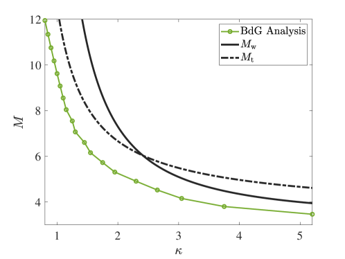
Figure 8: $M^{\ast}$ vs. $\kappa$. The two curves from Derrick’s Theorem lie above the numerically determined curve for instability to set in. See also, Fig. 2(a).

8 Conclusions

In this paper we have revisited the problem of blowup in the nonlinear Schrödinger equation with arbitrary nonlinearity exponent $\kappa$. In particular, we used the result that an arbitrary initial ground state wavefunction can be converted into an exact solution if we place it in a well-determined external potential. We find that in this confining potential the wavefunction can become unstable to both width and translation perturbations. There are two different onset masses at which this happens, with the translational instability occurring at a lower/higher mass than the width instability depending on whether $\kappa$ is less than or greater than $1+\sqrt{2}$. The numerical BdG analysis gives a curve for the critical mass that lies slightly below both these curves although it follows a similar trend. In the 4CC variational approximation, there are now several regimes with quite different behavior. When there is no confining potential, $\kappa d\geq 2$ defines the regime where there can be a blowup.

The case we study in detail here is $d=2$, so that $\kappa=1$ is the critical value of $\kappa$. What we find for the case when we are in the confining potential, when $\kappa<1$, one can not have blowup (or collapse) because of energy conservation, but there are now three distinct regimes. When we are below both critical masses, there is a regime of small oscillation response to small perturbations of the initial conditions. As we cross the threshold for $q$ instability, then we can have “frustrated” blowup where $G$ first oscillates and then the growth of $q$ causes the wavefunction to start spiking. However energy conservation prevents blowup from completing. Then one gets a sort of repetition of this pattern. When one crosses the second instability, there is a combination of oscillatory regions at low $G$ combined with peaking and collapsing.

The wavefunction can also oscillate about different values of $q$ both positive and negative. Once $\kappa\geq 1$, we have mainly two regimes. When we are below the two critical masses, we have oscillatory response to small perturbations. Once the $q$ instability is present, it then triggers blowup of the wavefunction. When one is below the second critical mass, the width makes one oscillation before one starts the blowup regime, as $q$ increases exponentially in time. We expect these types of behavior to exist irrespective of the exact choice of the initial approximate wavefunction used to describe the soliton in the absence of the external potential. In the stable regime, which is the small oscillation regime of the variational approximation, agreement with numerical simulation of the NLSE is quite good. However in the unstable regime, once the values of the first and second moments of the wavefunction start deviating in a substantial way from their initial values, other degrees of freedom get excited and our simple 4CC ansatz does not capture the behavior of the wavefunction very well.

Appendix A Extension to arbitrary dimension

In an arbitrary number of spatial dimensions $d$, one can assume arbitrary finite norm initial data and again find the potential that will lead to this initial data being an exact solution. If we take the initial data to be of the form

$$\psi(r,0)=A\,u(r)\>,$$ (1.1)

where $A$ is the amplitude, and then assume that the time-dependent solution is of the form:

$$\psi(r,t)=A\,u(r)\,\rme^{-\rmi\,\omega t}\>.$$ (1.2)

Then since the Laplacian in $d$ dimensions for radial solutions is

$$\nabla^{2}\psi(r,t)=\frac{\partial^{2}\psi(r,t)}{\partial r^{2}}+\frac{(d-1)}{r}\frac{\partial\psi(r,t)}{\partial r}\>,$$ (1.3)

we find from (2.1) that $u(r)$ satisfies

$$\omega+\frac{u^{\prime\prime}}{u}+\frac{(d-1)}{r}\frac{u^{\prime}}{u}+g\,A^{2\kappa}\,u^{2\kappa}=V(r)\>.$$ (1.4)

By choosing

$$\omega+\Bigl{[}\,\frac{u^{\prime\prime}}{u}+\frac{(d-1)}{r}\frac{u^{\prime}}{u}\,\Bigr{]}_{r=0}=0\>,$$ (1.5)

we are able to remove the constant term from the potential when $g=0$. This way, upon solving Eq. (1.5) for $\omega$ and substituting this back into Eq. (1.4), it gives an equation for the potential

$$V(r)=\Bigl{[}\,\frac{u^{\prime\prime}}{u}+\frac{(d-1)}{r}\frac{u^{\prime}}{u}\,\Bigr{]}_{\mathrm{sub}}+g\,A^{2\kappa}\,u^{2\kappa}\>,$$ (1.6)

where we have subtracted the derivative terms at $r=0$. It will be useful when discussing stability to rewrite the amplitude $A$ of the exact solution in terms of the mass $M$. In general the form of $A^{2}$ is $A^{2}=M/[\,C_{1}(d)\,\Omega(d)\,]$, as we will demonstrate below. Then we can rewrite $V(r)$ in the form.

$$V(r)=\Bigl{[}\,\frac{u^{\prime\prime}}{u}+\frac{(d-1)}{r}\frac{u^{\prime}}{u}\,\Bigr{]}_{\mathrm{sub}}+g\,\Bigl{[}\frac{M}{C_{1}\,\Omega}\Bigr{]}^{\kappa}\,u^{2\kappa}\>.$$ (1.7)

As an example, for a Gaussian initial data

$$\psi(r,t)=A\,\rme^{-\alpha\,r^{2}/2-\rmi\,\omega t}\>,$$ (1.8)

we find that the potential is now given by

$$V(r)=g\,A^{2\kappa}\,\rme^{-\kappa\,\alpha\,r^{2}}-\alpha\,d+\alpha^{2}\,r^{2}+\omega\>.$$ (1.9)

Thus, if we choose

$$\omega=\alpha\,d\>,$$ (1.10)

we find that the Gaussian is an exact solution provided that

$$V(r)=gA^{2\kappa}e^{-\kappa\alpha r^{2}}+\alpha^{2}\,r^{2}\>.$$ (1.11)

We can rewrite this in terms of the $mass$ of the solution. We have

$$\rho(r,t)=A^{2}\,\rme^{-\alpha\,r^{2}}\>,$$ (1.12)

and

$$M=\Omega(d)\int_{0}^{\infty}\,\mathrm{d}r\,r^{d-1}\rho(r,t)=A^{2}\Bigl{(}\frac{\pi}{\alpha}\Bigr{)}^{d/2}\,\Omega(d)\>,$$ (1.13)

where $\Omega(d)=2\pi^{d/2}/\Gamma(d/2)$, so that

$$V(r)=g\,M^{\kappa}\,\Bigl{(}\frac{\alpha}{\pi}\Bigr{)}^{\kappa d/2}\,\rme^{-\kappa\,\alpha\,r^{2}}+\alpha^{2}\,r^{2}\>.$$ (1.14)

This external potential makes the Gaussian an exact solution of the $d$-dimensional NLSE with arbitrary nonlinearity exponent $\kappa$.

Appendix B Acknowledgments

FC, EGC, and JFD would like to thank the Santa Fe Institute and the Center for Nonlinear Studies at Los Alamos National Laboratory for their hospitality. AK is grateful to Indian National Science Academy (INSA) for awarding him INSA Senior Scientist position at Savitribai Phule Pune University, Pune, India. The work at Los Alamos National Laboratory was carried out under the auspices of the U.S. Department of Energy and NNSA under Contract No. DEAC52-06NA25396.

References

References

- [1] M. Kono and M.M. Skorić, Nonlinear Physics of Plasmas, Springer-Verlag, Heidelberg, 2010.
- [2] Y.S. Kivshar and G.P. Agrawal, Optical Solitons: from fibers to photonic crystals, Academic Press, San Diego, 2003.
- [3] T. Dauxois and M. Peyrard, Physics of Solitons, Cambridge University Press, Cambridge, 2006.
- [4] M.J. Ablowitz, Nonlinear Dispersive Waves: Asymptotic Analysis and Solitons, Cambridge University Press, Cambridge, 2011.
- [5] L.P. Pitaevskii and S. Stringari, Bose-Einstein Condensations, Oxford University Press, Oxford, 2003.
- [6] C.J. Pethick and H. Smith, Bose-Einstein condensation in dilute gases, Cambridge University Press, Cambridge, 2002.
- [7] C. Sulem and P.L. Sulem, The Nonlinear Schrödinger Equation, Springer-Verlag, New York, 1999.
- [8] H.A. Rose and M.I. Weinstein, On the bound states of the nonlinear Schrödinger equation with a linear potential, Physica D: Nonlinear Phenomena 30 (1988), 207–218. doi:https://doi.org/10.1016/0167-2789(88)90107-8. http://www.sciencedirect.com/science/article/pii/0167278988901078.
- [9] F. Cooper, C. Lucheroni and H. Shepard, Variational method for studying self-focusing in a class of nonlinear Schrödinger equations, Physics Letters A 170 (1992), 184–188. doi:https://doi.org/10.1016/0375-9601(92)91063-W. http://www.sciencedirect.com/science/article/pii/037596019291063W.
- [10] J.M. Ball, Finite Time Blowup in Nonlinear Problems, Quart. J. Math., Oxford 28 (1977), 473–486. ISBN ISBN 0-12-195250-9.
- [11] N. Antar and N. Pamuk, Exact Solutions of two-Dimensional Nonlinear Schrödinger Equations with External Potentials, App. Comp. Math. 2(6) (2013), 152–158. doi:10.11648/j.acm.20130206.18.
- [12] S.J. Liao, The Proposed Homotopy Analysis Technique for the Solution of Nonlinear Problems, PhD thesis, Jiao Tong University, Shanghai, 1992.
- [13] J.H. He, Homotopy Perturbation Technique, Comp. Meth. App. Mech. Eng. 178(3–4) (1999), 257–262. doi:10.1088/1751-8113/40/29/015.
- [14] C. Sulem and P.-L. Sulem, The Nonlinear Schrödinger Equation: Self-Focusing and Wave Collapse, 139, Springer, Berlin, 2013. ISBN ISBN 13:9781475773071.
- [15] G.H. Derrick, Comments on Nonlinear Wave Equations as Models for Elementary Particles, J. Math. Phys. 5(9) (1964), 1252–1254. doi:10.1063/1.1704233.
- [16] J.F. Dawson, F. Cooper, A. Khare, B. Mihaila, E. Arevalo, R. Lan, A. Comech and A. Saxena, Stability of new exact solutions of the nonlinear Schrödinger equation in a Póschl-Teller external potential, J. Phys. A 50 (2017), 505202. doi:10.1088/1751-8121/aa9006.
- [17] P.A.M. Dirac, Note on exchange phenomena in the Thomas atom, Math. Proc. Camb. Philos. Soc. 26(3) (1930), 376–385.
- [18] P.A.M. Dirac, Wave Mechanics, Advanced General Theory, Clarendon Press, Oxford, 1934, p. 436.
- [19] V.M. Perez-Garcia, Self-similar solutions and collective coordinate methods for Nonlinear Schrödinger Equations, Physica D 191 (2004), 211–218.
- [20] R.T. Glassey, On the blowing up of solutions to the Cauchy problem for nonlinear Schrödinger equations, J. Math. Phys. 18 (1977), 1794–1797. doi:10.1063/1.523491.
- [21] P.G. de Gennes, Superconductivity of Metals and Alloys, Vol. 86, Benjamin, New York, 1966.