Proposal for a neutrino telescope in South China Sea

Abstract

Cosmic rays were first discovered over a century ago, however the origin of their high-energy component remains elusive. Uncovering astrophysical neutrino sources would provide smoking gun evidence for ultrahigh energy cosmic ray production. The IceCube Neutrino Observatory discovered a diffuse astrophysical neutrino flux in 2013 and observed the first compelling evidence for a high-energy neutrino source in 2017. Next-generation telescopes with improved sensitivity are required to resolve the diffuse flux. A detector near the equator will provide a unique viewpoint of the neutrino sky, complementing IceCube and other neutrino telescopes in the Northern Hemisphere. Here we present results from an expedition to the north-eastern region of the South China Sea. A favorable neutrino telescope site was found on an abyssal plain at a depth of $\sim$ 3.5 km. Below 3 km, the sea current speed was measured to be $v_{\mathrm{c}}<$ 10 cm/s, with absorption and scattering lengths for Cherenkov light of $\lambda_{\mathrm{abs}}\simeq$ 27 m and $\lambda_{\mathrm{sca}}\simeq$ 63 m, respectively. Accounting for these measurements, we present the preliminary design and capabilities of a next-generation neutrino telescope, The tRopIcal DEep-sea Neutrino Telescope (TRIDENT). With its advanced photon-detection technologies and size, TRIDENT expects to discover the IceCube steady source candidate NGC 1068 within 2 years of operation. This level of sensitivity will open a new arena for diagnosing the origin of cosmic rays and measuring astronomical neutrino oscillation over fixed baselines.

1 Introduction

Cosmic rays from deep space constantly bombard the Earth’s atmosphere, producing copious amounts of GeV – TeV neutrinos via hadronic interactions. Similar processes yielding higher energy (TeV – PeV) neutrinos are expected when cosmic rays are accelerated and interact in violent astrophysical sources, such as in jets of active galactic nuclei (AGN) [1]. Ultra-high-energy cosmic rays (UHECRs) traversing the Universe and colliding with the cosmic microwave background photons, are predicted to generate ‘cosmogenic’ neutrinos (beyond EeV) [2]. Detecting astrophysical neutrino sources will therefore be the key to deciphering the origin of the UHECRs.

The weak interactions which make neutrino detection so difficult, also allow them to be used as a powerful tool. They can escape from extremely dense environments, travelling astronomical distances without being deflected or absorbed. Pointing back directly to their sources of origin, neutrinos are a unique messenger to trace the most extreme regions of the Universe. Furthermore, neutrinos oscillate as they propagate through spacetime, transforming among flavours $\nu_{e}$, $\nu_{\mu}$ and $\nu_{\tau}$, due to the quantum effect known as flavor-mass mixing [3]. Measuring neutrino oscillation over astronomical baselines allows us to probe for new physics beyond the Standard Model [4], while also providing new handles for tests on quantum gravity [5].

Neutrinos cannot be detected directly. These ‘ghostly’ particles are measured using extremely sensitive technologies, detecting the charged particles generated in neutrino-matter interactions. In a general detector setup, large areas of photon-sensors continuously monitor a large body of target mass, e.g. pure water [6], liquid scintillator [7], liquid argon [8], to measure these rare and tiny energy depositions. Neutrino telescopes use large volumes of wild sea/lake water or glacial ice to observe the low rate of incident high energy astrophysical neutrinos.

Theoretical calculations in 1998 suggested that a cubic-kilometer detector would be sufficiently sensitive to the high energy neutrino flux from AGN jets or GRBs [9]. The IceCube Neutrino Observatory was the first experiment to build a telescope of this scale, instrumenting the deep glacial ice at the South Pole. IceCube made major breakthroughs over its lifetime, in 2013, discovering a diffuse extraterrestrial neutrino flux [10] and in 2017 detecting the first compelling evidence for neutrino emission from a flaring blazar [11, 12]. Dedicated analyses have been carried out to resolve the origins of the observed cosmic neutrino flux. A wide range of hypotheses have been considered, including: all-sky spatial clustering searches [13], transient searches [14, 15, 16] and AGN catalog stacking searches [17, 18], all yielding inconclusive results to date. This suggests multiple weaker sources [19] may contribute to the diffuse flux, such as star burst galaxies [20], which would require better than $0.1^{\circ}$ pointing resolution to resolve [21].

Several telescopes such as KM3NeT in the Mediterranean Sea [22], Baikal-GVD in Lake Baikal [23] and the newly proposed P-ONE in the East Pacific [24], are currently under development. Their northern locations will complement IceCube in the South Pole, offering full coverage of the TeV - PeV neutrino sky. Due to the Earth’s rotation, placing a detector near the equator would provide steady visibility of the entire neutrino sky, providing a unique contribution to the global network of neutrino observatories. Also, due to the reduced light scattering in water compared to the glacial ice of IceCube, neutrino telescopes built in deep seas and lakes will have substantial improvement in neutrino pointing. The combined efforts of these future experiments will yield a dramatic increase in the number of measured astrophysical neutrinos, allowing for the identification of their sources and significantly progress the field of neutrino astronomy.

We propose a next-generation neutrino telescope to be built in the South China Sea (TRIDENT), which aims to discover multiple high-energy astrophysical neutrino sources and provide a significant boost to the measurement of cosmic neutrino events of all flavors. We report on a scouting expedition conducted in the South China Sea in September 2021. We then discuss the key characteristics and optical properties of the selected site. A preliminary design of the envisioned telescope is also presented. Finally, we demonstrate the capabilities and sensitivity of this prospective telescope, using in-depth simulation studies that incorporate the measured on-site conditions.

2 Site investigation on oceanographic conditions

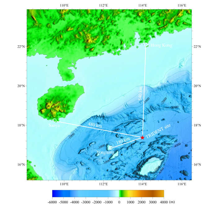
Figure 1: The selected site is marked by the red star. The distance between the TRIDENT site and nearby cities are shown by the white lines. The nearest island with infrastructure, Yongxing Island, is $\sim 180~{}\mathrm{km}$ away.

A suitable site for constructing a deep-sea neutrino telescope demands multiple conditions. The depth should be large enough, e.g. $\gtrsim 3~{}\mathrm{km}$, to effectively shield cosmic ray backgrounds and minimize the influence of biological activities. Experiences from the pioneer DUMAND project suggested that, a large and flat area such as an abyssal plain is preferred, and it should keep away from high rises or deep trenches to avoid complex current fields. The ocean floor should be flat and possess sufficient bearing strength to support the mounting of the equipment. Based on the successful operation of ANTARES for the past decade, a deep-sea neutrino telescope could safely operate under the current strength less than $\sim 20~{}\mathrm{cm/s}$ [25]. The proximity to a shore is required to ensure the infrastructure for power supply and data transmission via seafloor cable connections.

A pre-screening of viable sites with existing geographic and oceanographic data suggests that an area near 114.0^∘E, 17.4^∘N, located at the center of a large abyssal plain of depth $\sim 3500~{}\mathrm{m}$, is deep enough to largely avoid biological activities and provide sufficient overburden to shield cosmic ray muons down to $\sim 10^{-8}$ cm^-2s^-1sr^-1 [26]. The seabed of this area is very flat with a slope of 0.01 degrees and mainly covered by clay silt [27], which is suitable for building a large scale deep-sea detector. The location is about $180~{}\mathrm{km}$ from the nearest island with infrastructure, where placing detector’s power supply and experimental data storage on the island is feasible (see Figure 1). A geographic location close to the equator permits the detector to scan the whole sky once per day with its most sensitive zenith band. With these prior knowledge, we carried out the TRIDENT pathfinder experiment (TRIDENT EXplorer, T-REX for short) at the selected site. With T-REX, we measured the optical properties of the sea water and also quantified the oceanographic conditions of the chosen site, including water current, salinity and radioactivity.

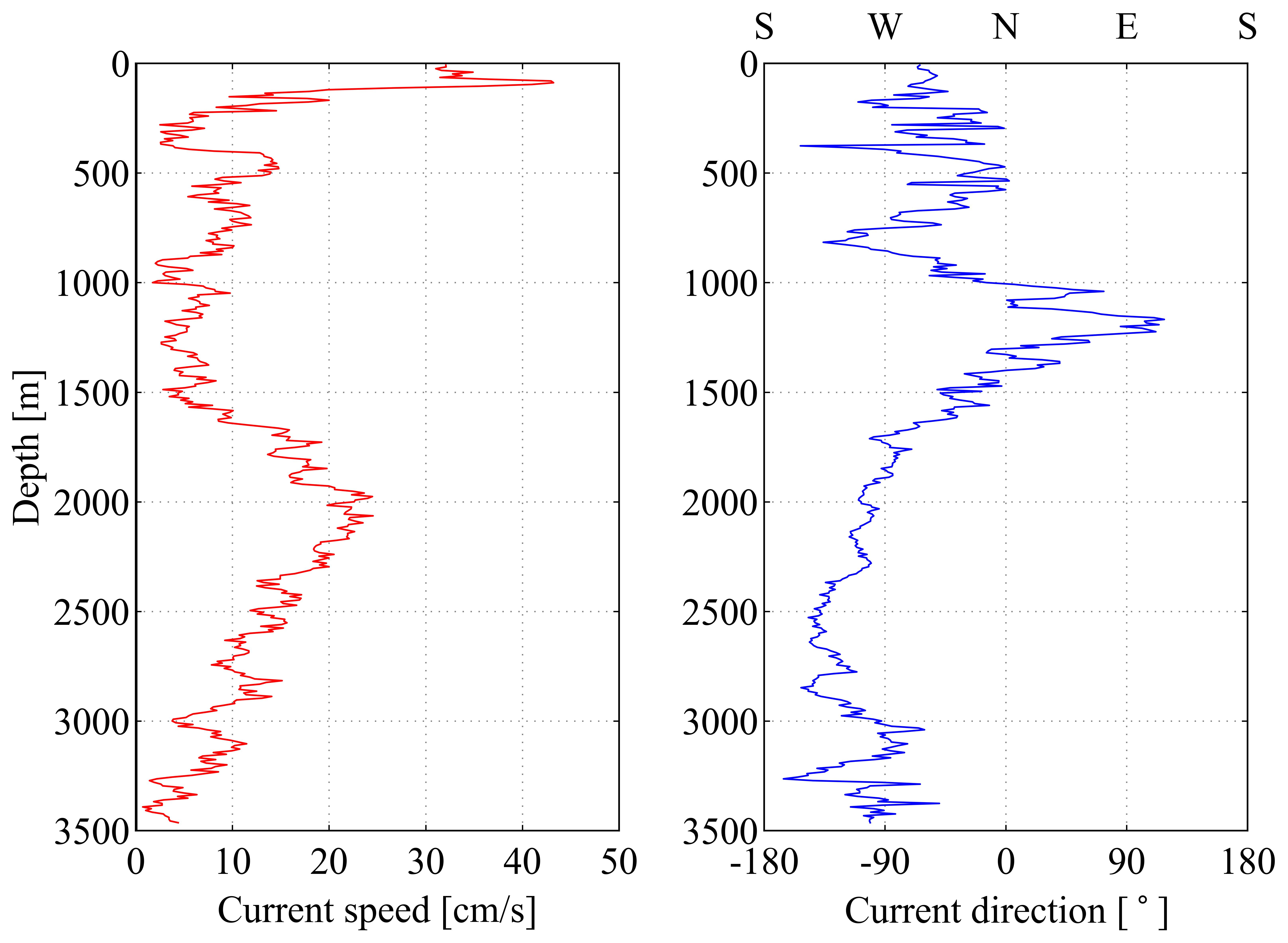
Figure 2: Current speed and direction as a function of depth. The data was taken on September 6, 2021.

The water current at different depths at the chosen site was measured by the LADCP (Lowered Acoustic Doppler Current Profiler) on September 6, 2021. Figure 2 shows the water current with respect to depth. Below $\sim 2800~{}\mathrm{m}$, the water current speed is less than $10~{}\mathrm{cm/s}$. The current is steady and changes slowly in time. Additionally the temperature and salinity, measured by a CTD (Conductivity, Temperature and Pressure), are shown in Figure 3. Below $2500~{}\mathrm{m}$, the temperature becomes constant at $\sim 2^{\circ}\mathrm{C}$. Furthermore, a submerged buoy equipped with multiple sensors was deployed for a year-long continuous monitoring of the site.

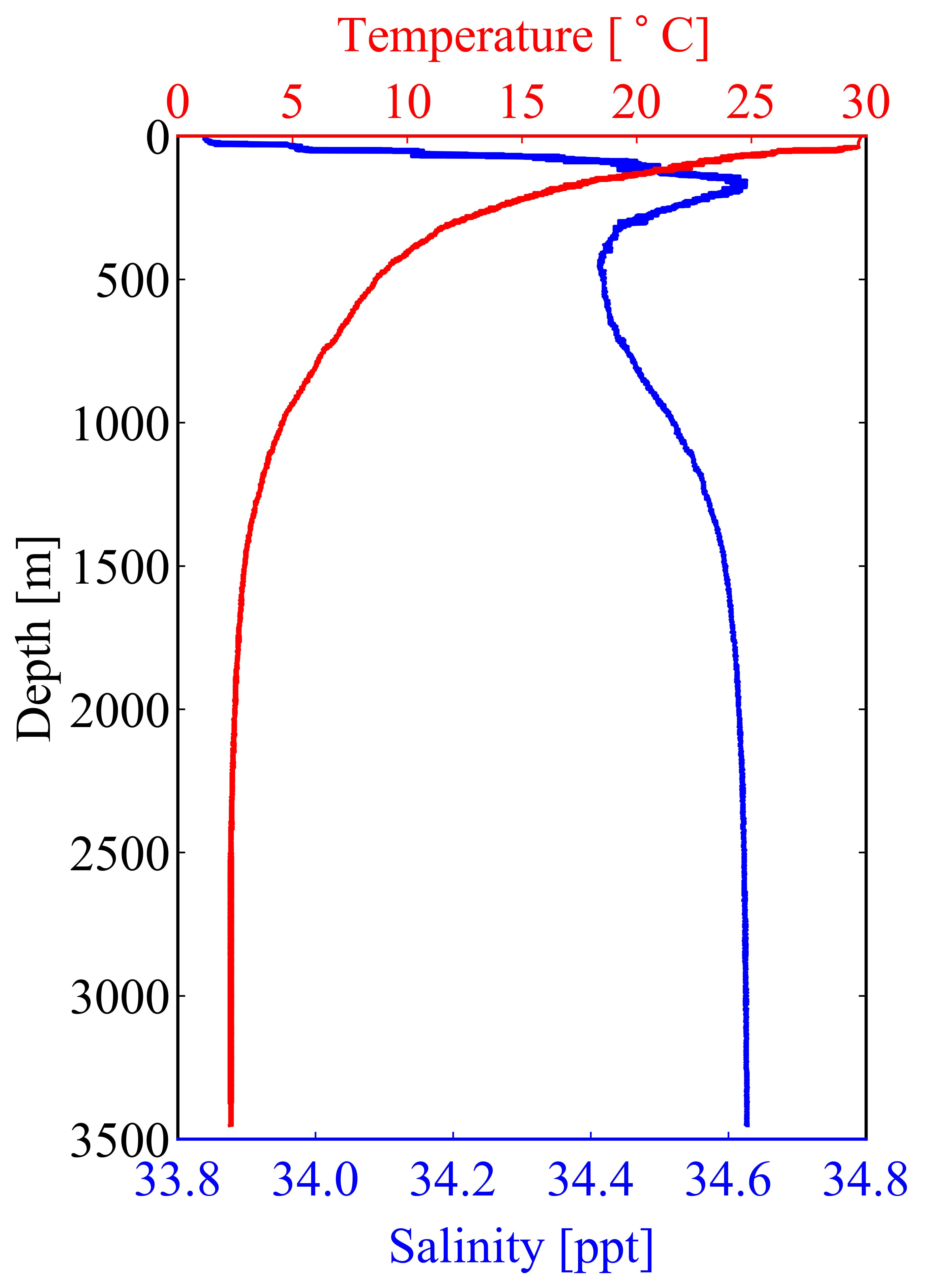
Figure 3: Left panel: water density and sound speed as a function of depth. Right panel: temperature and salinity as a function of depth. The data was taken on September 6, 2021.

3 Site investigation on optical properties

3.1 Optical properties of the deep-sea water

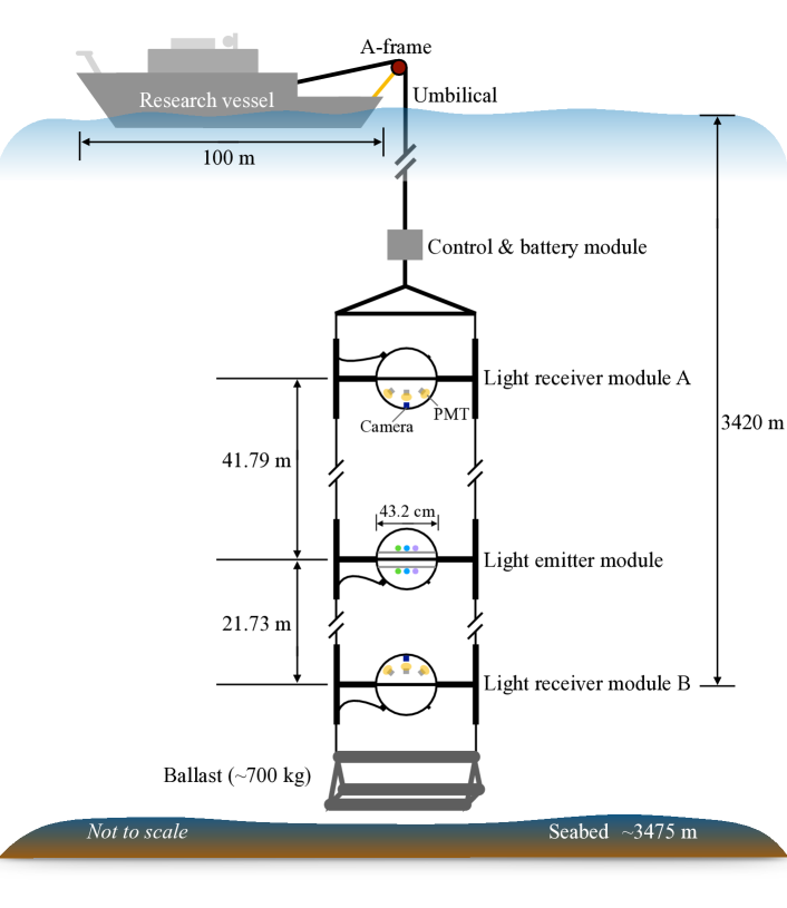
Figure 4: A schematic plot of the T-REX apparatus. The apparatus was deployed to a depth of $3420~{}\mathrm{m}$ by the umbilical cable from a research vessel. A light emitter module is placed in the middle. Light receiver module A and B are placed on the top and bottom at a distance of $41.79\pm 0.04~{}\mathrm{m}$ and $21.73\pm 0.02~{}\mathrm{m}$ respectively. Each module is connected to the control and battery module via a composite optical-electric cable for data communications and power supply. This figure is not to scale.

One of the most important criteria for site selection is the optical property of the water, since neutrino telescopes observe neutrinos by detecting the Cherenkov photons generated in the medium. By measuring the number of these photons and their arrival times, information about the primary neutrino involved in the interaction can be reconstructed.

The propagation of Cherenkov photons is predominantly affected by the absorption and scattering processes. Absorption converts the photon energy into atomic heat via photon-molecule interactions [28]. This reduces the total number of observable photons. Scattering, on the other hand, causes photons to change their direction of propagation.This leads to a blurring of arrival times for Cherenkov light arriv ing at photon detection units, thus degrading the angular resolution of the neutrino telescope. The deflection angle of scattering process is characterized by the so-called scattering phase function [28]. In sea water, Rayleigh and Mie scattering are dominant and both are elastic scattering processes [29]. Rayleigh scattering occurs when the scattering particles are smaller than the incident photon’s wavelength, e.g. bound electrons of water molecules. Its phase function is relatively homogeneous and can be modeled by $1+\cos\theta_{\mathrm{Ray}}^{2}$, where $\theta_{\mathrm{Ray}}$ denotes the scattering angle [29]. The Mie scattering process becomes significant when the size of the scatterers, e.g. dust or other particulates suspending in the medium, are approximately equal to or larger than the photon wavelength. Its phase function is skewed in the forward direction and needs an extra parameter $\left\langle\cos\theta_{\mathrm{Mie}}\right\rangle$ to represent the mean scattering angle [29]. The strength of absorption, Rayleigh scattering and Mie scattering can be quantified by their mean free path, denoted as $\lambda_{\mathrm{abs}}$, $\lambda_{\mathrm{Ray}}$ and $\lambda_{\mathrm{Mie}}$, respectively. In most cases in seawater, the absorption and scattering processes are combined together. In this case, another optical parameter, attenuation length $\lambda_{\mathrm{att}}$, is introduced to describe the exponential decrease in the intensity of a light beam in the medium, which can be decomposed as $\lambda_{\mathrm{att}}=1/(1/\lambda_{\mathrm{abs}}+1/\lambda_{\mathrm{sca}})$. However, for a spherical isotropic light source, it is easier to measure an effective attenuation length, $\lambda_{\mathrm{eff,att}}$, which describes the decrease in the total number of photons $\propto e^{-D/\lambda_{\mathrm{eff,att}}}\cdot D^{-2}$, for a propagation distance $D$ [30]. Such a $\lambda_{\mathrm{eff,att}}$ differs from the canonical attenuation length $\lambda_{\mathrm{att}}$ because the scattered photons are also included in the observed light.

3.2 Design of the T-REX apparatus

In order to decode all these optical parameters, precise in-situ measurements were conducted with T-REX, as shown in Figure 4. The core detection unit consists of three modules. At the middle is a light emitter module installed with LEDs of various wavelengths ($405~{}\mathrm{nm}$, $450~{}\mathrm{nm}$, $460~{}\mathrm{nm}$, $525~{}\mathrm{nm}$). These can emit photons isotropically with two emission modes: pulsing mode and steady mode. The two light receiver modules are located at $21.73\pm 0.02~{}\mathrm{m}$ and $41.79\pm 0.04~{}\mathrm{m}$ vertically away from the light emitter respectively. Both are equipped with two independent and complementary measurement systems, a PMT and camera system. The former mainly records waveforms to extract the timing information of the detected photons emitted by pulsing LEDs, while the latter records images of the steady light emitter to measure the angular distribution of radiance. The combined system is designed to perform a near-far relative measurement.

3.3 Data taking and analyses

In order to safely deploy the long and delicate apparatus, it was first packed on the deck like a wire roller, then hoisted into the water. It then unfolded naturally under the action of its buoyancy and gravity. The ballast at the bottom weighs about $700~{}\mathrm{kg}$, and the connection cables between the detection modules are made of high-rigidity steel wires to ensure that the low-frequency disturbance of the research vessel will not excite the resonance of the system.

During the deployment process, periodical tests were firstly conducted by the camera system at the fixed depths of $1221~{}\mathrm{m}$ and $2042~{}\mathrm{m}$. Each test took $8~{}\mathrm{minutes}$ to record data. After reaching the target depth of $3420~{}\mathrm{m}$, the whole apparatus was suspending for $\sim$ 2 hours to conduct in-situ measurements. The data taking was then divided into two stages. The light emitter was first operated in the pulsing mode to trigger the PMT system. For the wavelength of $450~{}\mathrm{nm}$, it took about $50~{}\mathrm{minutes}$ to collect more than $10^{7}$ photons. The data collection for other two wavelengths, namely $405~{}\mathrm{nm}$ and $525~{}\mathrm{nm}$ lasts $10~{}\mathrm{minutes}$ for quick measurements. In the second stage, the camera system recorded more than 3000 images when the light emitter was switched to steady mode with wavelengths of $460~{}\mathrm{nm}$, $525~{}\mathrm{nm}$ and $405~{}\mathrm{nm}$ in sequence and the entire camera data taking process lasted about $30~{}\mathrm{minutes}$. After completing the measurements at the depth of $3420~{}\mathrm{m}$, the whole apparatus was retrieved for recycle.

3.3.1 PMT data analysis

During the PMT data taking stage, PMTs and pulsing LEDs are synchronically triggered by the White Rabbit system at a rate of $10~{}\mathrm{kHz}$. The PMTs are designed to operate at $\sim 1375~{}\mathrm{V}$ with a gain of $\sim 10^{7}$. The PMT signals are digitized by a $250~{}\mathrm{MHz}$ analog-to-digital converter (ADC) in a $1000~{}\mathrm{ns}$ data acquisition (DAQ) window. Figure 5 shows a typical PMT waveform.

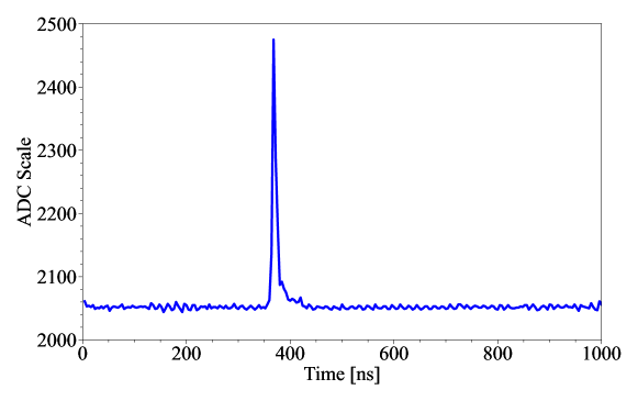
Figure 5: A typical PMT waveform. For each pulse of the LEDs, the PMT data is acquired in a window of length $1000~{}\mathrm{ns}$. The PMT waveform is digitized with a 250 MHz sampling frequency, and a DAQ window length of 1000 ns is represented by an array of 250 ADC values. The ADC value spans from 0 to 4095, corresponding to the voltage range from -875.0 $\mathrm{mV}$ to +875.0 $\mathrm{mV}$.

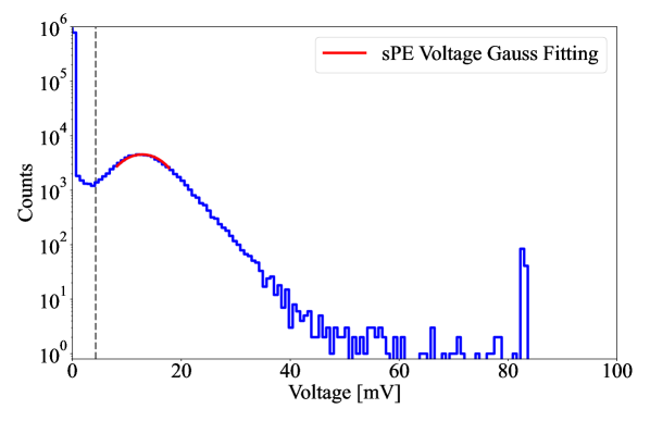
Figure 6: After getting the baseline ADC value, the waveform of ADC values can be transformed into a waveform of PMT signal voltages. The voltage is calculated by $V=\frac{(A-A_{b})\times V_{0}}{M_{\text{pre}}}$, where $A$ is the ADC value, $A_{b}$ is the baseline ADC value, $V_{0}$ is $0.43~{}\mathrm{mV}$ per ADC point, and $M_{\text{pre}}=10.5$ is the pre-amplification factor. The spe peak is well fitted by a Gaussian distribution.

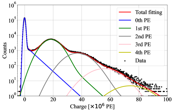
Figure 7: A typical charge spectrum. The charge integral of a PMT waveform is calculated by $Q_{w}=\sum_{j=1}^{250}{\frac{V(j)}{R_{\text{PMT}}}\delta t}$, where $V(j)$ is the PMT signal voltage of the waveform, $R_{\text{PMT}}=50\Omega$ is the resistance of the PMT base, $\delta t=4$ ns is the time per ADC point. The obtained distribution, so called charge spectrum, which can be fitted by a convolution of Poisson and Gaussian functions [31].

Analysis of the PMT data consists of two steps. First, the photon arrival time distribution for each PMT is reconstructed. Then, the photon arrival time distribution is fitted with light propagation models simulated by Geant4 for optical parameters.

Reconstruction of the photon arrival time distribution is calculated as follows. First, the average voltage amplitude for the single-photoelectron (spe) signal $V_{\mathrm{spe}}$ is determined by the mean value of the Gaussian distribution (see Figure 6). Next, the gain of the PMT $G_{\mathrm{spe}}$ is determined by fitting the charge spectrum with a standard model [31] (see Figure 7). Then, pulses whose amplitudes exceed $\frac{1}{3}V_{\mathrm{spe}}$ are regarded as signal pulses. After that, the charge of each signal pulse $Q_{\mathrm{pulse}}$ and the number of photons by $N_{\gamma}=\frac{Q_{\mathrm{pulse}}}{G_{\mathrm{spe}}}$ is obtained. The time of each pulse is weighted by $N_{\gamma}$ for all events to obtain the photon arrival time distribution, shown in Figure 8.

The model used to fit the photon arrival time distribution is composed of (1) emission from the pulsing LEDs; (2) propagation in the water; (3) detection by the PMTs. This can be written as:

$$[N_{\mathrm{emi}}\times f(t)]\otimes[\frac{A}{4\pi D^{2}}\times P(t\,|\,\lambda_{\mathrm{abs}},\lambda_{\mathrm{Ray}},\lambda_{\mathrm{Mie}},\left\langle\cos\theta_{\mathrm{Mie}}\right\rangle,n,D)]\otimes[\eta\times g(t)],$$ (1)

where $N_{\mathrm{emi}}$ is the number of emitted photons, $f(t)$ is the LED pulse timing profile, $A$ is the effective detection area of the PMT, $P(t\,|\,\lambda_{\mathrm{abs}},\lambda_{\mathrm{Ray}},\lambda_{\mathrm{Mie}},\left\langle\cos\theta_{\mathrm{Mie}}\right\rangle,n,D)$ is the photon propagation function, $D$ is the distance, $\eta$ and $g(t)$ are the PMT detection efficiency and time response, respectively. The convolution of the LED pulse profile and PMT time response $f(t)\otimes g(t)$ is measured in the lab. The final model is computed by convolving the simulated photon propagation distribution and calibrated LED and PMT time response.

A $\chi^{2}$ fitting method is adopted to fit the photon arrival time distribution with the above model for a pair of PMTs from the top and bottom receiver modules:

$${\chi}^{2}=\sum_{i=1}^{N}{\frac{(D_{i}-M_{i}-\sum_{k=1}^{K}{c_{k}\cdot\beta_{ki}})^{2}}{{\sigma_{i}}^{2}}}+\sum_{k=1}^{K}{{c_{k}}^{2}},$$ (2)

where $D_{i}$ is number of data counts in the $i^{th}$ bin of the photon arrival time distribution histogram and $M_{i}$ is the expected value by the model. The overall uncorrelated uncertainty $\sigma_{i}$ includes statistical fluctuation, electronic noise and uncertainty in the LED pulse profile and PMT time response. $\beta_{ki}$ is the contribution from the $k^{th}$ correlated uncertainty. These include fluctuations in LED brightness, distances, PMT gains, PMT detection efficiencies, as well as the binning effect caused by the $4\,\text{ns}$ ADC resolution. In total, 5 physics parameters contribute to the $\chi^{2}$ calculations: $\lambda_{\mathrm{abs}}$, $\lambda_{\mathrm{Ray}}$, $\lambda_{\mathrm{Mie}}$, $\left\langle\cos\theta_{\mathrm{Mie}}\right\rangle$, and refraction index $n$. Minimization of the ${\chi}^{2}$ will return the best-fit parameters and their uncertainties.

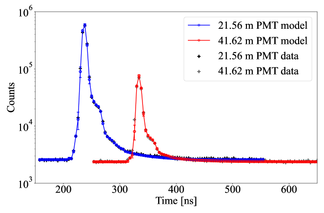
Figure 8: Measured photon arrival time distribution with a fit to photon arrival time model. The photon arrival time model is obtained by Geant4 simulation, with the LED and PMT response taken into account.

For cross validation, a Markov Chain Monte Carlo (MCMC) technique is also used to obtain the best model using the emcee sampler [32]. The goal of MCMC is to approximate the posterior distribution of model parameters by random sampling in a probabilistic space. A multi-dimension linear interpolation is performed before the sampling since the model in our case is discrete.

It should be noted that both the $\chi^{2}$ fitting and MCMC methods follow the same procedures described above but have minor differences in the detailed treatment of convolution. Despite this, the two methods yield consistent results. Three pairs of PMTs from the top and bottom light receivers are used to fit the the optical parameters independently, where consistency is also seen between each.

The effective attenuation length can be derived by comparing the mean number of photons $N_{\mathrm{hit}}$ received by top and bottom PMTs. Here, $N_{\mathrm{hit}}$ is the integral of photon arrival time distribution over $1000~{}\mathrm{ns}$ DAQ window. A simulation study shows that $\sim 25\%$ and $\sim 45\%$ of photons in $N_{\mathrm{hit}}$ have encountered a scatter process at least once in the near and far PMT respectively, making the measurement result deviate from the canonical attenuation length, as discussed in Section 3.1. Such contamination cannot be eliminated by reducing the integration time window.

3.3.2 Camera data analysis

The camera system mainly consists of a 5-million-pixel monochromatic camera with a fixed-focus lens. It’s controlled by a Raspberry-4Pi module which can transfer its real-time data back to the research vessel. In seawater both top and bottom cameras (denoted as CamA and CamB ) are calibrated to get a proper viewing angle of about $16^{\circ}$. During the data-taking process, we set the same series of exposure times ($0.02~{}\mathrm{s}$-$0.2~{}\mathrm{s}$) for all wavelengths to accommodate for the blind conditions in the deep water. Moreover, short exposure times can also prevent motion blur caused by sea current perturbations affecting the whole apparatus. The camera system only works with the steady mode of the light emitter and thus can easily get enough statistics of photons. The major observable for a camera is the angular distribution of the radiance, which is converted into gray values of pixels.

The first method for camera system, named as $I_{\mathrm{center}}$ method, is used to quickly measure the attenuation length of the medium by comparing the gray values in the central region of light emitter images:

$$\lambda_{\text{att}}=-(D_{A}-D_{B})/\ln(-\frac{I_{\text{A}}}{I_{\text{B}}}\cdot\frac{I_{0}^{\prime}}{I_{0}}).$$ (3)

Here, $D_{A}-D_{B}$ is the relative distance between the two cameras. $I_{\mathrm{A}}$ and $I_{\mathrm{B}}$ are the mean gray values in the center region of images from CamA and CamB, corresponding to the directly arriving light from the emitter. $I_{0}^{\prime}/I_{0}$ is the initial gray value ratio of both sides of the light emitter, which is well calibrated. The canonical attenuation length can be derived from such a setup due to the far distance between the camera and light emitter makes the light beam highly collimated, with an open angle of $<1.1^{\circ}$ for CamA and $<0.6^{\circ}$ for CamB, thus both the absorption and the scattering will dissipate the radiance. A Geant4 simulation study calculates that there is a small contamination of scattered photons, roughly 2%, in the measured light beams. This contamination ratio is approximately equal in both the near and far cameras, thus does not have influence on the $I_{\mathrm{center}}$ method.

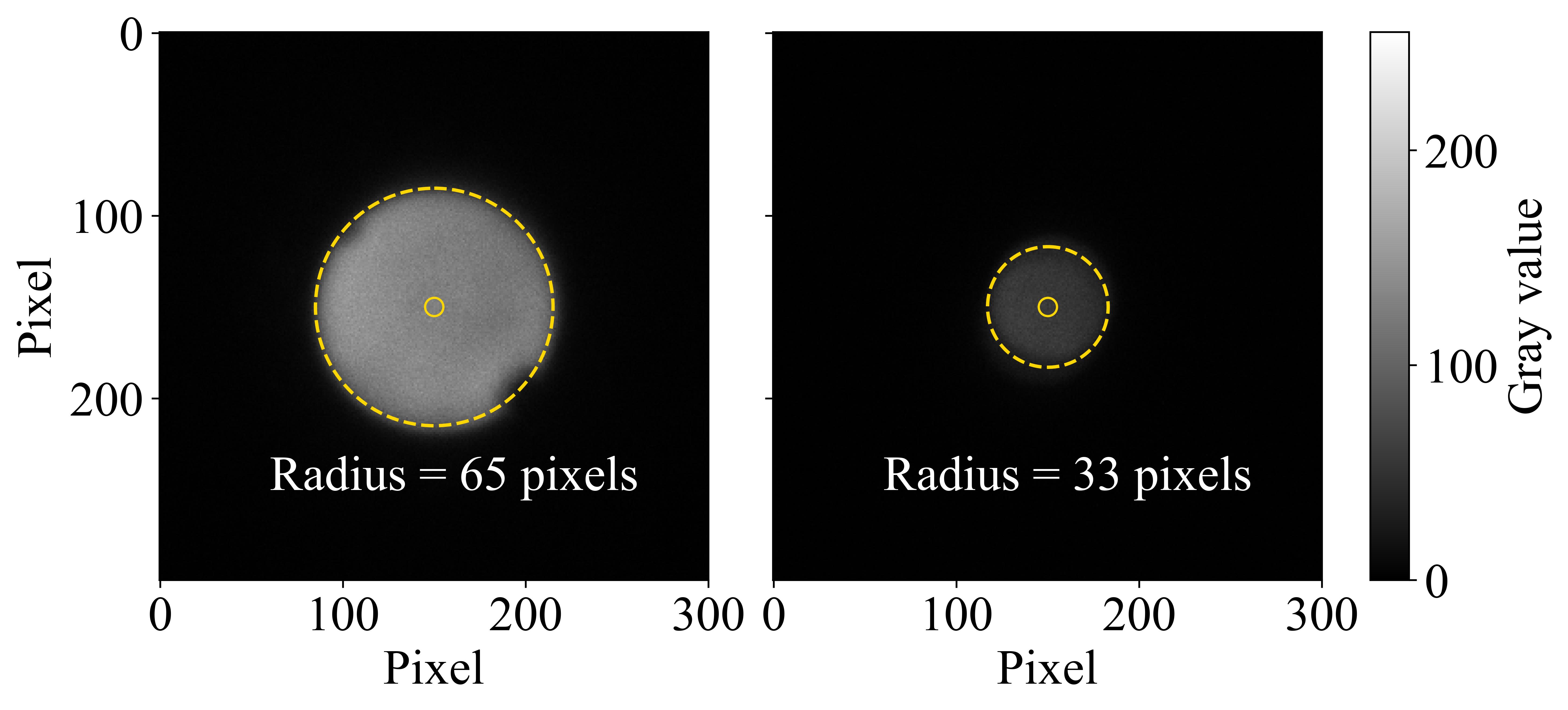
Figure 9: Images of the light emitter at a wavelength of $460~{}\mathrm{nm}$ with an exposure time of $0.02~{}\mathrm{s}$ and a water depth of $3420~{}\mathrm{m}$. The dashed circle shows the profile of the light emitter and the gray value distribution of the inside region is used for the $\chi^{2}$ fitting analysis. The region enclosed by the solid circle is used for the analysis of the $I_{\mathrm{center}}$ method. Left panel: an image taken by CamB at a distance of $21.5~{}\mathrm{m}$, the radius of the dashed circle is 65 pixels. Right panel: an image taken by CamA at a distance of $41.6~{}\mathrm{m}$, the radius of the dashed circle is 33 pixels.

The image processing procedure mainly consists of the following: (1) Select images with proper exposure time and gain settings, in which all the pixels for analysis are not saturated. For our 8-bit cameras, the maximum gray value of a single pixel is 255. When the gray values of most of pixels are between 20-230, our cameras show excellent linear response, not only from the results of our pre-calibration, but also the self-calibration in deep sea. (2) Find the centroid of each image then cut to a unified size of $300\times 300$ pixels, shown in Figure 9, to include all the directly arriving light. (3) Calculate the mean gray value with 100 central pixels around the centroid from both CamA and CamB images as $I_{\text{A}}$ and $I_{\text{B}}$ in formula 3 then calculate the final attenuation length.

The uncertainty estimation for the $I_{\text{center}}$ method firstly includes conventional systematic or statistical errors from the pre-calibration results of $I_{0}^{\prime}/I_{0}$, the relative distances and the gray value calculation. Systematic uncertainties such as luminosity loss at air-glass-water interface are canceled out in this setup.

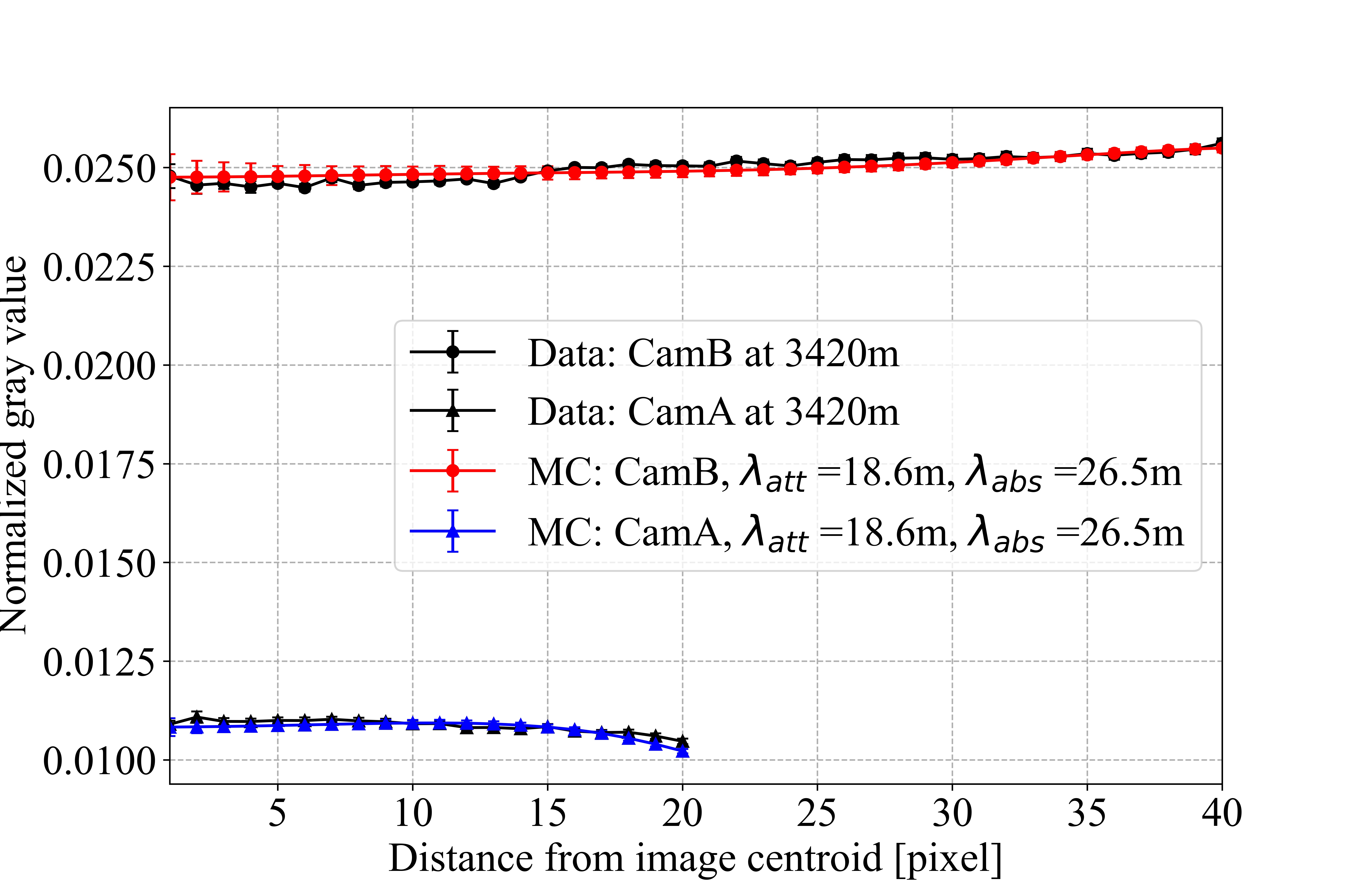
Figure 10: The $\chi^{2}$ fitting analysis of the camera system is to compare the gray value distribution of central pixels between the experimental data and simulated data generated by Geant4. By minimizing the $\chi^{2}$, the best-fit simulated data with a specific $\lambda_{\text{att}}$ and $\lambda_{\text{abs}}$ can be obtained as shown in this figure.

In order to distinguish the absorption and scattering length from the attenuation process respectively, we present the $\chi^{2}$ fitting method that compares the angular distribution of radiance between experimental data and the simulated data, as shown in Figure 10. This method consists of the following : (1) Select images and cut them off using just the same procedure introduced in $I_{\text{center}}$ method. (2) Normalize both experimental data and simulated data of CamA and CamB but with the same normalization factor to keep the ratio of gray values of the center area. (3) Convert 2D images into a 1D gray value array by calculating the mean gray value of those pixels which have the same pixel distance from the centroid. (4) Choose the first 40 and 20 points in the gray value arrays of CamA and CamB to calculate the sum of $\chi^{2}$ pixel by pixel with the model:

$$\chi^{2}=\sum_{i=1}^{N}{\frac{[M_{i}-T_{i}(1+\sum_{k=1}^{K}{\epsilon_{k}})]^{2}}{\sigma_{Mi}^{2}+\sigma_{Ti}^{2}}}+\sum_{k=1}^{K}{\frac{{\epsilon_{k}^{2}}}{\sigma_{k}^{2}}}.$$ (4)

Here, $M_{i}$ is the measured data in the $i$th pixel bin while $T_{i}$ is the model prediction. $\sigma_{Mi}$ and $\sigma_{Ti}$ are both uncorrelated uncertainties coming from statistical fluctuation. $\epsilon$ is added to include uncorrelated systematic uncertainties such as the uncertainties in distances and the calibration result of $I_{0}^{\prime}/I_{0}$. Other uncertainties such as the slight de-focusing of the imaging process and the non-uniformity of the light emitter were all included in simulation and added as nuisance parameters when calculating $\chi^{2}$.

The effective attenuation length can not be obtained from the experimental images like PMT system due to the limited viewing angle of our cameras. However, based on the best-fit simulated data from $\chi^{2}$ fitting, the effective attenuation length can be calculated by modifying the $I_{\mathrm{center}}$ method with a numerical factor representing the effect of scattered photons.

4 Results

4.1 Optical properties of the TRIDENT site

Table 1 summarizes the results from both the PMT and camera systems at wavelengths of $450~{}\mathrm{nm}$ and $460~{}\mathrm{nm}$, the optimal waveband for observing Cherenkov photons. Although two systems measure their own observables and are sensitive to different optical parameters, their results are consistent. Furthermore, for each system we adopt two analysis methods for independent validation. All of the data processing and analysis pipelines are presented in detail in Section 3.3. Additionally, the results for other two wavelengths measured by PMT system and different depths measured by camera system are listed in Table 2 of A and Table 3 of B, respectively.

To compare our results with other similar measurements for water-based neutrino telescopes, we conducted another set of analyses to obtain $\lambda_{\text{eff,att}}$ because definitions of attenuation length in other experiments slightly differ from us. Because of the time response uncertainties for both light source and PMTs, the results from LAMS [33] and STRAW-a [34] are effective attenuation lengths because scattered photons are also included in the selected DAQ windows regardless of the duration. A detailed investigation on this effect was performed in a Geant4 simulation. The results from Baikal-5D, however, made measurements of canonical attenuation lengths, using a specialized device [35]. Results from the discussion above are shown in Figure 11.

PMT (at $\sim$ 450 nm)
Method	$\lambda_{\text{abs}}$ [m]	$\lambda_{\text{ray}}$ [m]	$\lambda_{\text{mie}}$[m]	$\cos\theta_{\text{mie}}$	$\lambda_{\text{att}}$ [m]	$\lambda_{\text{att,eff}}$ [m]
$\chi^{2}$ fitting	$27.4^{+1.1}_{-0.9}$	$200^{+13}_{-10}$	$84^{+12}_{-8}$	$0.97^{+0.02}_{-0.02}$	$18.7^{+3.0}_{-2.1}$	$24.8\pm 2.4$
MCMC	$26.4^{+1.2}_{-1.0}$	$203^{+15}_{-11}$	$64^{+12}_{-14}$	$0.97^{+0.01}_{-0.01}$	$17.2^{+0.8}_{-1.3}$
Camera (at $\sim$ 460 nm)
Method	$\lambda_{\text{abs}}$ [m]	$\lambda_{\text{sca}}$ [m]			$\lambda_{\text{att}}$ [m]	$\lambda_{\text{att,eff}}$ [m]
$\chi^{2}$ fitting	$26.5\pm 0.5$	$62.9\pm 3.7$			$18.7\pm 0.2$	$26.8\pm 2.6$
$I_{\text{center}}$	$\lambda_{\text{att}}=19.3\pm 1.3$

Table 1: Results of optical property measurements at depth of $3420~{}\mathrm{m}$ for both PMT ($450~{}\mathrm{nm}$) and camera ($460~{}\mathrm{nm}$) systems of T-REX.

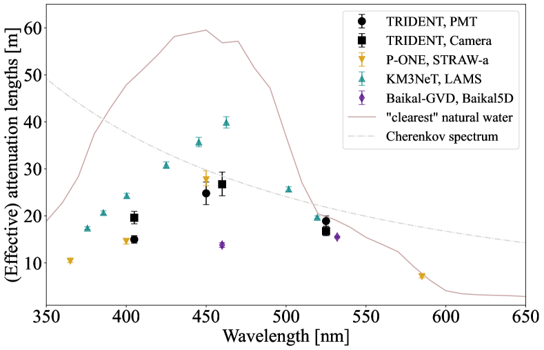
Figure 11: Effective attenuation lengths measured by two independent optical systems, the PMT (black circle) and camera (black square) of T-REX for three wavelengths (405 nm, 450/460 nm, 525 nm). Other optical measurements, including KM3NeT [33], P-ONE STRAW-a [34] and Baikal-GVD [35] are shown for comparison. Also shown are the attenuation lengths of the ‘clearest’ nature water measured in the Sargasso Sea [36].

4.2 Radioactivity

To precisely measure the radioactivity of the site, in-situ water was collected with CTD and transported back to Shanghai through cold chain logistics. The radioactivity (dominantly ⁴⁰K) of the water was then measured by the PandaX team using high purity germanium detector [37] in the China Jinping Underground Laboratory. The measured abundance of ${}^{40}\mathrm{K}$ is $10.78\pm 0.21~{}\mathrm{Bq/kg}$, consistent with public data of ordinary seawater. A background analysis with Geant4 simulation indicates that this level of radioactivity corresponds to a trigger rate of $\sim 4~{}\mathrm{kHz}$ per PMT (see Figure 12), acceptable for operating both T-REX and the future neutrino telescope. During the apparatus deployment and data taking periods, biological activity sometimes showed up and was recorded by our cameras above depth of $1500~{}\mathrm{m}$. No activity was spotted during the 2 hour camera data-taking period at a depth below $3000~{}\mathrm{m}$, indicating the site had appropriately low rates of bio-activity.

Figure 12: The hit rate in each PMT caused by ⁴⁰K radioactivity in Geant4 simulation. It converges to $\sim$4 kHz as the implemented spherical volume increases. The simulation setup is adapted from [38], in which the detector layout is the same as the light receiver module used in T-REX, and ⁴⁰K decay vertices are sampled uniformly within a spherical volume whose center is the detector and radius is a variable. The ⁴⁰K abundance is set to be 10.8 Bq/kg and their decay will produce Cherenkov photons that can hit on PMTs. The error bars in the graph are due to the limited statistics of simulation.

5 Towards a next generation neutrino telescope

The measured optical properties and water current speeds seem promising for operating a large scale neutrino telescope on the selected site. The camera system developed and tested for T-REX has been demonstrated to be an excellent real-time calibration tool, which can be adopted as an essential fast in-situ calibration system for future dynamic (water-based) neutrino telescopes. T-REX also served as a successful pilot test for some full-scale electronic systems to be used in TRIDENT, such as the use of time synchronization technologies and optical fibers for data transmission.

5.1 Conceptual design of TRIDENT

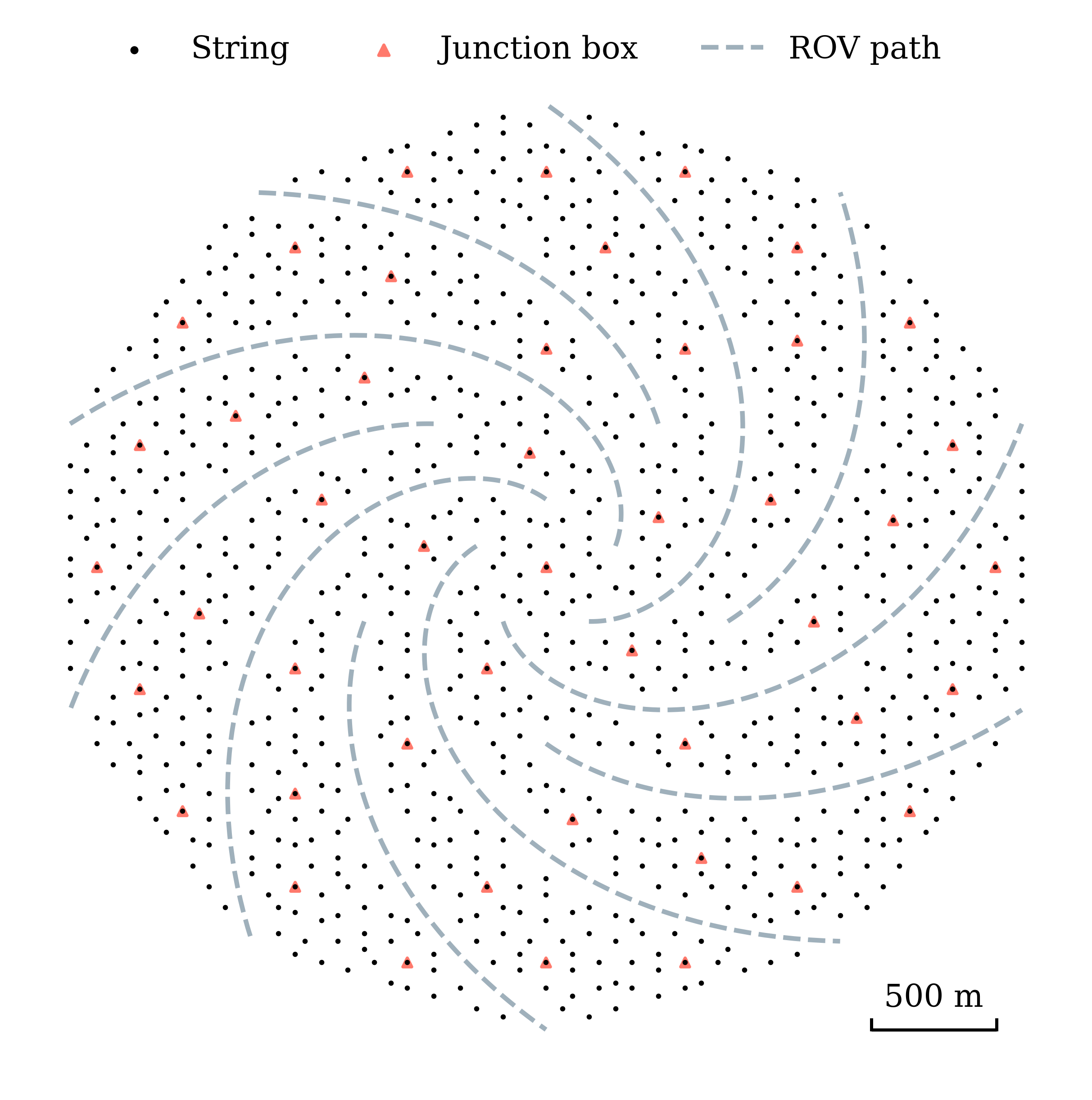
Figure 13: Geometry layout of the TRIDENT array. The pattern follows a Penrose tiling distribution. Each black dot represents a string of length of $\sim 0.7~{}\mathrm{km}$, while the dashed lines mark the paths for underwater maintenance robots.

A next-generation neutrino telescope should be optimized to pinpoint more astrophysical neutrino sources from the isotropic diffuse flux discovered by IceCube. The long scattering lengths in deep-sea water allow the Cherenkov photons from a neutrino interaction vertex to propagate in long straight paths to the many optical sensors throughout the detector. Precisely measuring the arrival times of these direct photons strongly improves the angular resolution of track-like events due to $\nu_{\mu}$ (and a fraction of $\nu_{\tau}$) charged current (CC) interactions, which neutrino telescopes rely primarily on for pointing [39]. This can be achieved with the help of modern SiPMs (Silicon Photon Multipliers) that can respond to photon hit within tens of picoseconds [40], the TDCs (Time Digital Converters) that is capable of digitizing the sharp raising edge of a SiPM waveform [41] and the White Rabbit system that can provide precise global time stamps [42]. TRIDENT will utilise these state-of-the-art technologies, building a hybrid digital optical module with both PMTs and SiPMs, called hDOM [43], yielding excellent light collection and timing resolution. Applying hDOM in the telescope will achieve $\sim 40\%$ improvement in angular resolution in comparison to traditional PMT only DOM [44], which would significantly boost it’s source searching capability.

Cherenkov photons are more likely to be absorbed than scattered in seawater. Therefore, the absorption length is the key parameter to consider when designing the layout of the detector geometry. Figure 13 shows a preliminary layout of the envisioned telescope, based on the presented optical property measurements. The pattern follows a Penrose tiling distribution with twofold inter-string distances, $70~{}\mathrm{m}$ and $110~{}\mathrm{m}$, which follows the golden ratio [45]. The uneven layout allows for an expanded geometry, monitoring a large volume of water target while remaining sensitive to low energy events. The design allows for a broad window of measurable neutrino energies, expected to cover from sub TeV to EeV, optimizing the telescope’s potential for neutrino astronomy [46]. The preliminary design of TRIDENT contains 1211 strings, each containing 20 hDOMs separated vertically by $30~{}\mathrm{m}$, resulting in an instrumented geometric volume of $\sim 7.5~{}\mathrm{km}^{3}$. Underwater robots will be used for the maintenance of the telescope. It is challenging, however, for these machines to navigate the dense array of strings. Several spiral pathways are left to mitigate difficulties in construction and maintenance, while also avoiding ‘corridor events’, which describe undetected muons passing straight through parallel arrays of strings. Acoustic detectors will be installed on each string for high-precision position calibration. These detectors can also be placed sparsely in an array extended beyond the main detector volume, to detect cosmogenic neutrinos with energies well above EeV [47, 48].

5.2 Source sensitivity and discovery potentials

We conducted a performance study of TRIDENT using track events. Those events are produced by $\nu_{\mu}$ CC interaction and its track like topology enables high-accuracy angular reconstruction, making them the golden channel for source searching. Furthermore, we only select up-going events that have zenith angle greater than $80^{\circ}$ and travel long distances inside the Earth, so that we can be free from the contamination of atmospheric muons.

A full detector simulation pipeline is built for this study. The Earth density and composition is constructed according to the Preliminary Earth Model [49]. The primary $\nu_{\mu}$ is injected near the detector following a similar scheme described in [50]: the $\nu_{\mu}$ are forced to interact with proper weightings around the detector and the $\mu$ generated are propagated into the detector. The high energy neutrino-nucleon deep inelastic scattering interaction cross-section developed by [51] is adopted in simulation. The produced $\mu$ and hadrons are then propagated into the detector using PROPOSAL [52] and sibyll [53]. Once the particles arrive at the detector, they are taken over by a fine-grained Geant4 simulation with energy cut down to $2~{}\mathrm{MeV}$. Cherenkov photons produced during Geant4 simulation will be propagated using GPU accelerated ray-tracing pipeline [54].

A multi-photon-electron algorithm [39] that utilizes both fast time resolution of Silicon Photomultipliers and large photon collection area of Photomultipliers Tubes [43] is used for track reconstruction. The angular resolution and effective area of TRIDENT are shown in Figure 14 and 15. At an energy of $\sim 100~{}\mathrm{TeV}$, the angular resolution of TRIDENT is expected to reach 0.1^∘ with an effective area of $7\times 10^{2}~{}\mathrm{m^{2}}$.

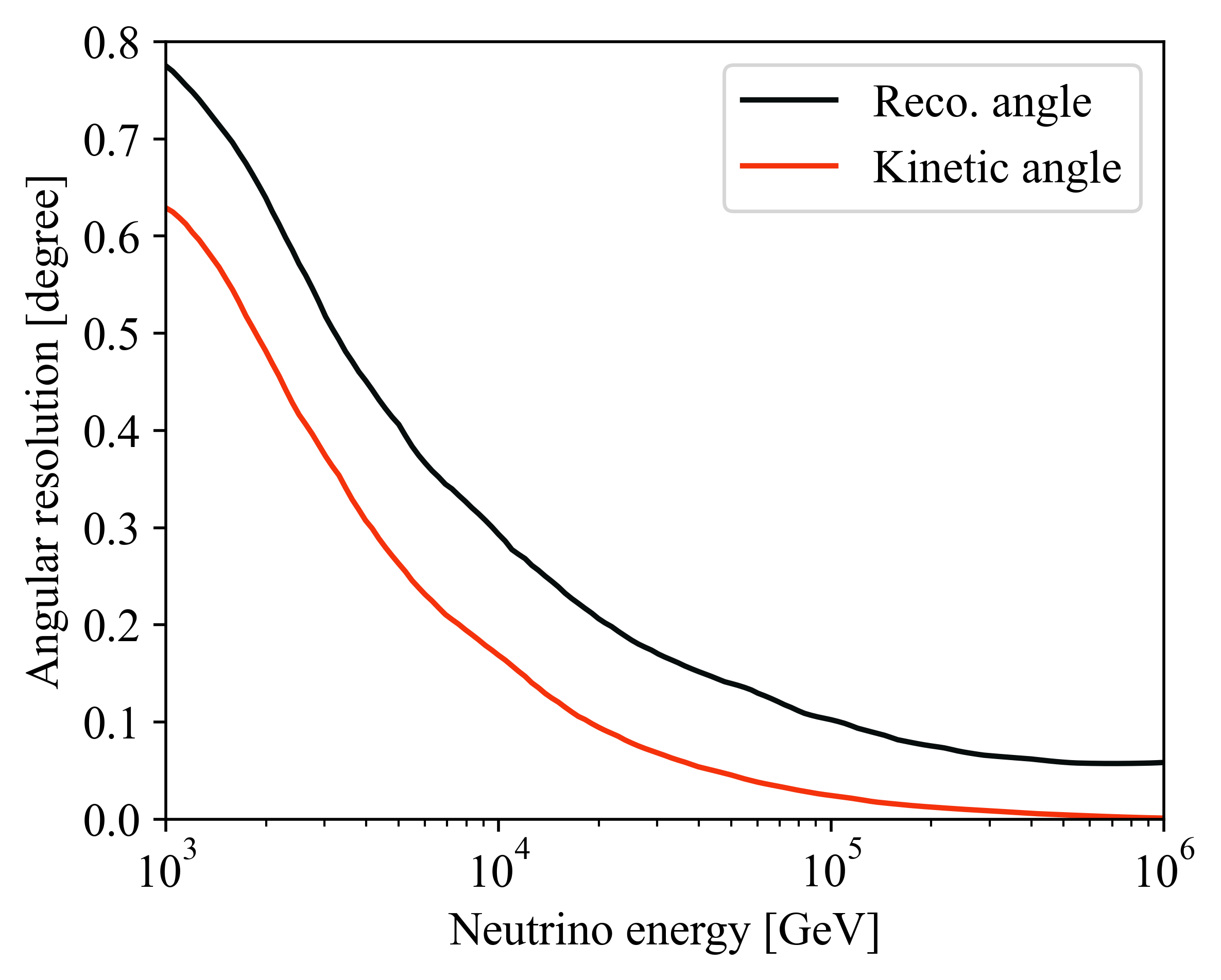
Figure 14: Median angular error as a function of the primary neutrino energy for $\nu_{\mu}$ track events. The black line represents the open angle between the reconstructed muon track direction and the primary neutrino direction. The red line is the open angle between the primary neutrino direction and the true muon direction. At an energy of $\sim 100~{}\mathrm{TeV}$, the angular error is expected to reach 0.1^∘.

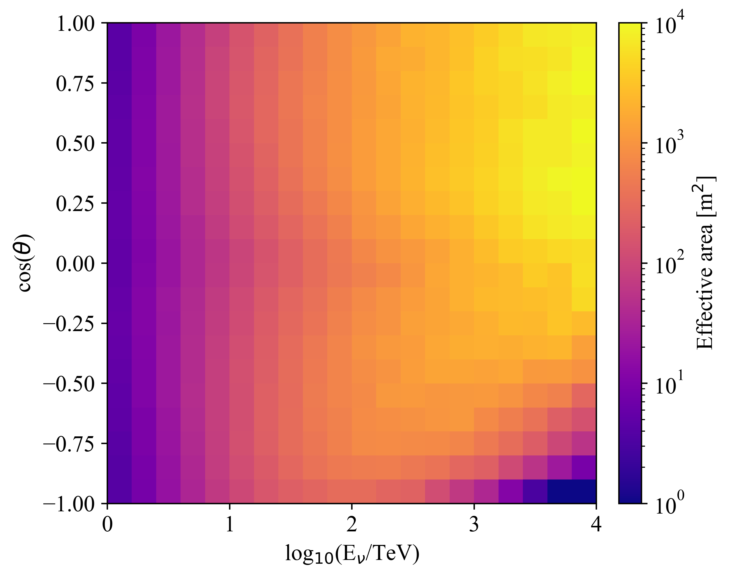
Figure 15: Effective areas at event reconstruction level for $\nu_{\mu}$ track events as a function of primary neutrino energy and zenith angle in TRIDENT. At an energy of $\sim 100~{}\mathrm{TeV}$, the effective area for up-going events is expected to reach $7\times 10^{2}~{}\mathrm{m^{2}}$. Only events with anglular error less than 6 degree are selected to evaluate the effective area.

With TRIDENT pushing the limits in neutrino telescope performance, the detector is expected to reach a new frontier in the sensitivity of all-sky searches for astrophysical neutrino sources. A point source sensitivity study is performed with respect to the diffuse astrophysical muon neutrinos [55] and atmospheric muon neutrinos backgrounds [56]. The results are shown in the upper panel of Figure 16. The most promising neutrino source candidates found by IceCube, NGC 1068 and TXS 0506+056 [13, 11, 12], will be visible to TRIDENT in the up-going neutrino mode, for $\sim$50% of its operation time. Assuming an IceCube best fit flux, TRIDENT is predicted to discover the steady source NGC 1068 within two years of operation, as shown in the lower panel of Figure  16. For a transient neutrino burst similar to the TXS 0506+056 2014-2015 case, TRIDENT will detect it with a significance level over $10\sigma$.

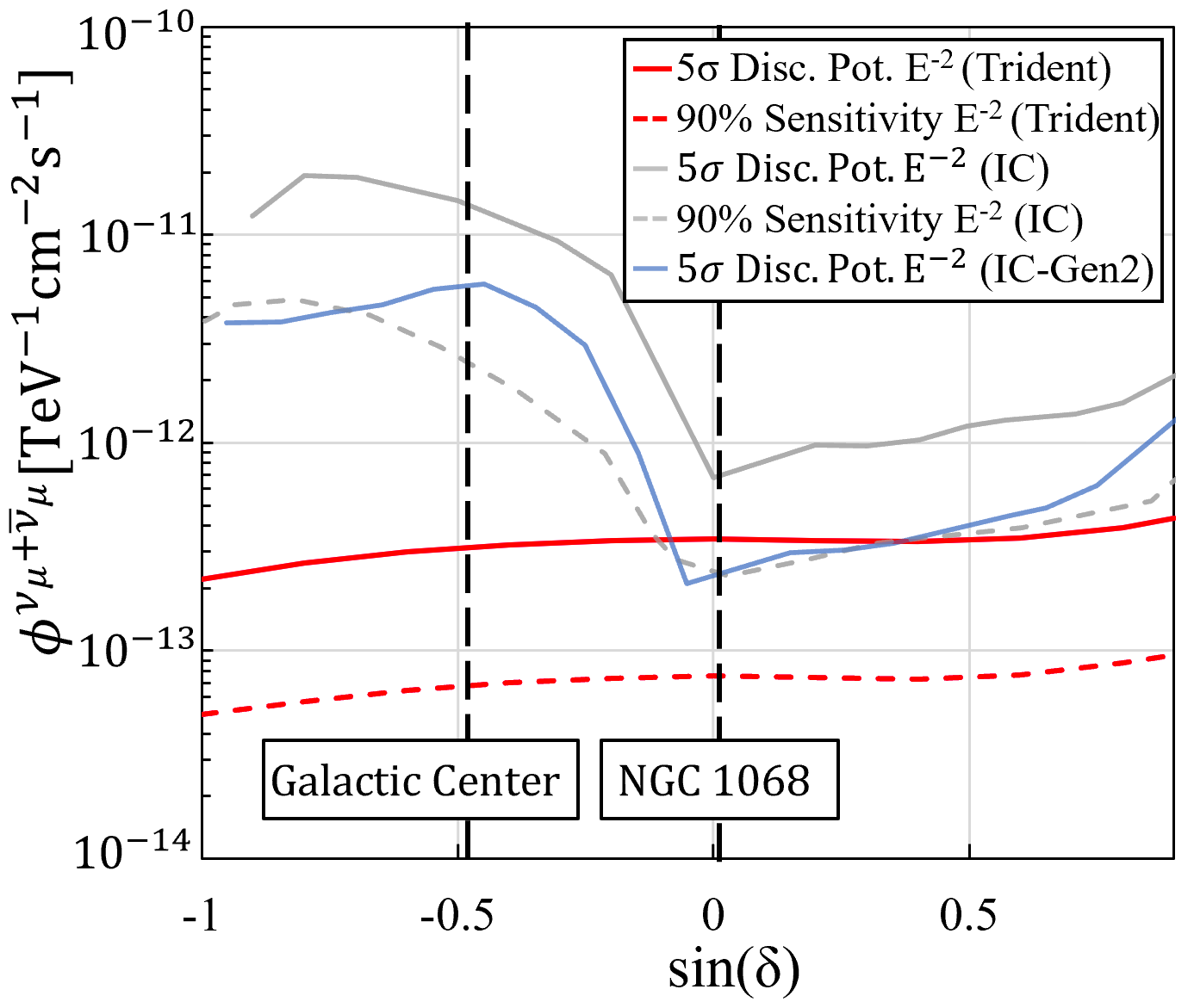
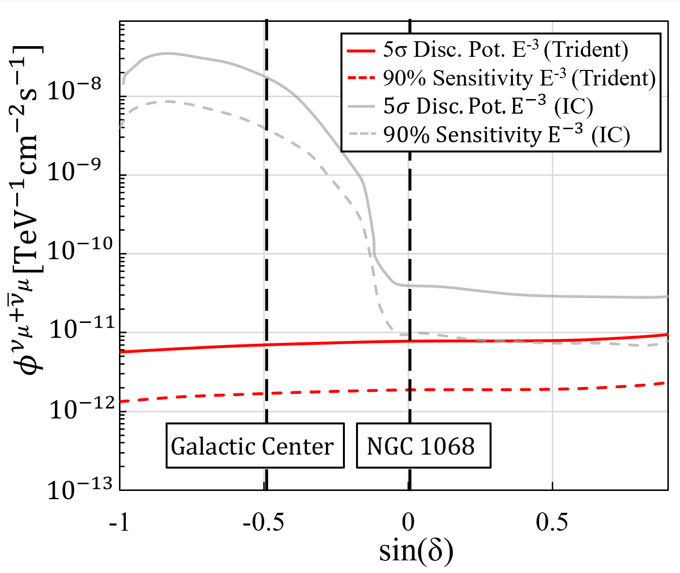
(a) All sky point source 90% C.L. median sensitivity and $5\sigma$ discovery potential for TRIDENT. The left panel corresponds to a source spectrum index of 2 and minimum energy of $10~{}\mathrm{TeV}$, while the right assumes an index of 3 and minimum energy of $1~{}\mathrm{TeV}$. The $x$ axis represents the sine declination. IceCube and IceCube-Gen2 sensitivities [13, 57] are also shown for comparison. For a source located at southern sky with spectrum index of 3, TRIDENT will have 4 orders of magnitude improvement in sensitivity compared to IceCube.

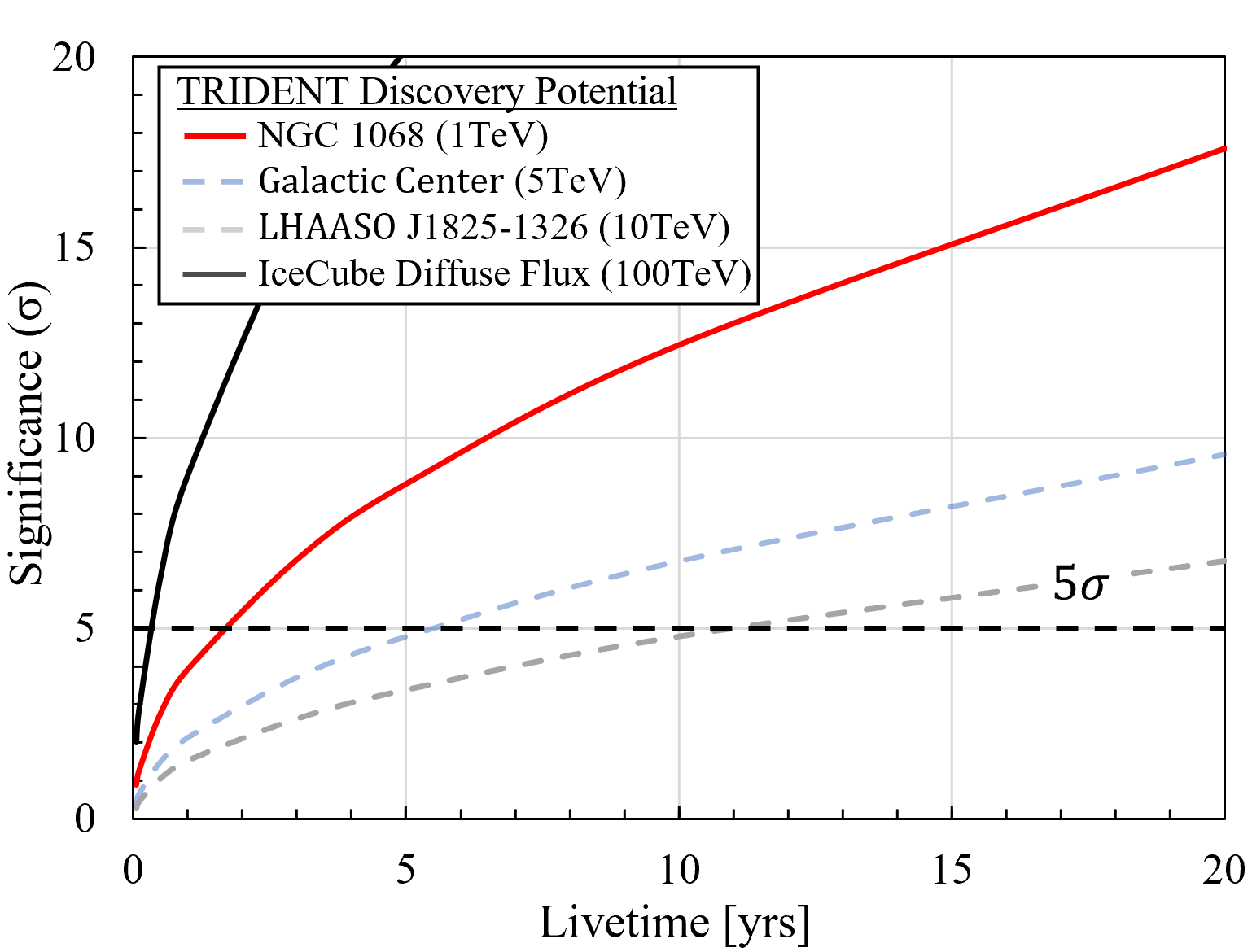
(b) The exposure time needed to discover potential neutrino sources. The source flux used in the analysis can be found in Table 4 in C. The minimum energies adopted for each source are shown in the legend.

Figure 16: Projected point source sensitivity and discovery potentials for TRIDENT.

5.3 Physics with all neutrino flavors

Once astrophysical neutrino sources are identified, oscillation physics and searches for new physics will become feasible by measuring the neutrino flavor ratio at fixed astronomical baselines. In particular, we expect to significantly boost the measurement of astrophysical tau neutrino events using modern long waveform readout electronics [58, 59] and also identify astrophysical electron antineutrinos via the Glashow resonance channel [60]. It is a particularly exciting time because IceCube has seen the first evidence for both types of events [61, 62, 63, 64]. Drastically boosting the statistics of these event types will produce a plethora of new physics opportunities. Another aspect to improve is the discrimination efficiency between electromagnetic and hadronic showers from $\nu_{e}$ CC interactions and neutral-current (NC) interactions of all flavors by their distinct particle compositions [65]. This will open unique windows via the weak sector to probe physics at an energy frontier out of reach by contemporary man-made accelerators [66].

5.4 Ocean engineering and timelines

It is not a trivial task to construct and operate such a giant array of precision detectors in a highly dynamic water body. Each string is mounted to the seafloor and raised by a buoy tied to the other end. Delicate efforts are required to achieve the correct buoyancy and cable strength, accounting for possible extreme conditions such as benthic storms in the abyss. We carried out the first batch of small-scale tests of the array-current response, using $1:250$ scale string toy models in a ship towing tank located on the campus of Shanghai Jiao Tong University. No significant horizontal displacement of strings was observed at a current of $<10~{}\mathrm{cm/s}$. More dedicated testing will be employed to guide the mechanical design of the strings. Modules monitoring the sea currents will be installed among the telescope array to track the instantaneous dynamics of the environment, ensuring smooth operation. In order to issue accurate real-time neutrino alerts, fast calibrations systems e.g. cameras, will be needed. These guarantee precise angular reconstruction as the detector’s environment changes. A pilot project with three strings installed in the selected site for a technology demonstration is scheduled for $\sim$ 2026. Construction of the full array can begin following a successful demonstration, commencing measurements in its partially built configuration. The full telescope is envisioned to become live in early 2030.

6 Summary and outlook

To substantially advance the field of neutrino astronomy, next generation neutrino telescopes with improved angular resolution and overall sensitivity are required to pinpoint more sources out of the diffuse flux discovered by IceCube. A neutrino telescope located near the Earth’s equator will have even visibility to the entire neutrino sky, adding unique strength to the global network of neutrino observatories.

We have presented the results from an expedition to scout for potential neutrino telescope sites in South China Sea. A flat area of $\sim$ 100 km² located at the north-eastern abyssal plain was found to meet the criteria for constructing a neutrino telescope. The depth is $\sim 3475~{}\mathrm{m}$, with water current speeds less than $10~{}\mathrm{cm/s}$ below $2800~{}\mathrm{m}$. An apparatus housing both PMT and camera systems was deployed from a research vessel to a depth of $3420~{}\mathrm{m}$ to collect data for the measurement of the in-situ optical properties of the deep-sea water. The absorption and scattering lengths near $460~{}\mathrm{nm}$ wavelength were measured to be $\lambda_{\mathrm{abs}}\simeq 27~{}\mathrm{m}$ and $\lambda_{\mathrm{sca}}\simeq 63~{}\mathrm{m}$, respectively.

Based on the measured parameters, we performed a preliminary design for a next generation neutrino telescope envisioned to be built at the selected site – The tRopIcal DEep-sea Neutrino Telescope (TRIDENT), aiming to rapidly identify several astrophysical neutrino sources when it gets online. TRIDENT will employ the state-of-the-art technologies such as SiPMs and long waveform readout electronics inside a hybrid optical module, bringing significant improvement in angular resolution for high-energy neutrinos and sensitivity to all neutrino flavors. The array of TRIDENT contains $\sim$ 1200 strings, monitoring a volume of $\sim 7.5~{}\mathrm{km^{3}}$. A two-fold uneven string spacing with the Penrose tiling will be adopted to expand the energy window of the detector and avoid the corridor events. Assuming an IceCube best fit flux, TRIDENT is predicted to discover the most promising steady source NGC 1068 within two years of operation, while for a transient neutrino burst similar to TXS 0506+056, TRIDENT will detect it with a significance level over $10\sigma$.

The design of TRIDENT will be studied in further details in future works. The horizontal distances between strings and the vertical distance between hDOMs will be further optimized. The simulation and reconstruction pipelines for all-flavor neutrinos are yet to be implemented. The design of the electronic systems for both the hDOM and the entire array are under way.

7 Acknowledgements

We are grateful to Frank Wilczek for his earnest support on jump starting this project. We are also appreciative for the helpful exchanges with Francis Halzen and Paschal Coyle on a number of issues involving stable operation of neutrino telescopes. Moreover, the authors thank Yifang Wang for the insightful conversations which have helped greatly in shaping of this project. The sea scouting team owes special gratitude to Shuangnan Zhang for his company and support during the voyage. We are obliged to Jie Zhang and Zhongqin Lin – the former and current president of Shanghai Jiao Tong University (SJTU), respectively – for their enthusiasm and enduring support for this proposal. Last but not least, we are much indepted to Dan Wu – the former vice president of SJTU — who helped assemble and coordinate the interdisplinary service team, without which this pathfinder experiment would not have been possible.

We thank the China Jinping Underground Laboratory for providing precise measurements of the seawater radioactivity. We are also grateful for the 1:2-million maps of the South China Sea and relevant data provided by the Guangzhou Marine Geological Survey, Ministry of Natural Resources of China. This work was sponsored by the National Natural Science Foundation of China (NSFC) under grants No. 12175137 and No. U20A20328, and by SJTU under the Double First Class startup fund and the Foresight grants No. 21X010202013 and No. 21X010200816. We acknowledge the Shanghai Pujiang Program (No. 20PJ1409300), and the sponsorship from the Hongwen Foundation in Hong Kong, and Tencent Foundation in China.

8 Author contributions

Ziping Ye, Fan Hu and Wei Tian contributed substantially and equally throughout the apparatus development and data analyses; Xinliang Tian designed the deployment device and led the marine operations; Donglian Xu proposed and led the development of this project; all authors have read and consent on the content.

Appendix A Optical properties measured by PMT system

PMT (at $\sim 405~{}\mathrm{nm}$)
Method	$\lambda_{\text{abs}}$ [m]	$\lambda_{\text{ray}}$ [m]	$\lambda_{\text{mie}}$[m]	$\cos\theta_{\text{mie}}$	$\lambda_{\text{att}}$ [m]	$\lambda_{\text{att,eff}}$ [m]
$\chi^{2}$ fitting	$20.8^{+1.0}_{-0.9}$	$120^{+12}_{-9}$	$55^{+20}_{-10}$	$0.98^{+0.02}_{-0.02}$	$13.4^{+5.1}_{-2.7}$	$15.0\pm 0.8$
MCMC	$19.2^{+0.5}_{-0.5}$	$114^{+4}_{-3}$	$46^{+6}_{-15}$	$0.98^{+0.01}_{-0.01}$	$12.1^{+0.4}_{-1.2}$
PMT (at $\sim 525~{}\mathrm{nm}$)
Method	$\lambda_{\text{abs}}$ [m]	$\lambda_{\text{ray}}$ [m]	$\lambda_{\text{mie}}$[m]	$\cos\theta_{\text{mie}}$	$\lambda_{\text{att}}$ [m]	$\lambda_{\text{att,eff}}$ [m]
$\chi^{2}$ fitting	$22.2^{+1.2}_{-1.0}$	$330^{+20}_{-15}$	$135^{+30}_{-20}$	$0.98^{+0.02}_{-0.02}$	$18.0^{+4.3}_{-2.9}$	$18.8\pm 1.1$
MCMC	$18.5^{+0.7}_{-0.6}$	$330^{+19}_{-22}$	$127^{+13}_{-22}$	$0.98^{+0.01}_{-0.01}$	$15.3^{+0.5}_{-0.5}$

Table 2: Results of optical property measurements from the PMT system of T-REX at wavelengths of $405~{}\mathrm{nm}$ and $525~{}\mathrm{nm}$ and at depth of $3420~{}\mathrm{m}$.

Appendix B Optical properties measured by camera system

Camera (at $\sim 460~{}\mathrm{nm}$)
Method	Depth [m]	$\lambda_{\text{att}}$ [m]
$I_{\text{center}}$	1221	$17.8\pm 1.1$
$I_{\text{center}}$	2042	$18.7\pm 1.2$
$I_{\text{center}}$	3420	$19.3\pm 1.3$
Camera (at $\sim 525~{}\mathrm{nm}$, depth of $3420~{}\mathrm{m}$)
Method	$\lambda_{\text{abs}}$ [m]	$\lambda_{\text{sca}}$ [m]	$\lambda_{\text{att}}$ [m]	$\lambda_{\text{att,eff}}$ [m]
$\chi^{2}$ fitting	$17.5\pm 0.5$	$57.2\pm 6.5$	$13.4\pm 0.2$	$16.7\pm 1.0$
$I_{\text{center}}$	$\lambda_{\text{att}}=14.6\pm 0.7$
Camera (at $\sim 405~{}\mathrm{nm}$, depth of $3420~{}\mathrm{m}$)
$I_{\text{center}}$	$\lambda_{\text{att}}=13.7\pm 0.6$			$19.5\pm 1.3$

Table 3: Results of attenuation lengths at $460~{}\mathrm{nm}$ in different depths and other optical parameters at $525~{}\mathrm{nm}$ and $405~{}\mathrm{nm}$ in depth of $3420~{}\mathrm{m}$ measured by camera system.

Appendix C Source spectrum used in the sensitivity analysis

Source	Description	References
NGC 1068	From IceCube best fit result	[13]
Galactic Center	Converted from the HESS gamma-ray observation assuming 100% hadronic origin	Yellow line in Figure 2 of [67]
LHAASO J1825-1326	Converted from the LHAASO gamma-ray observation assuming 100% hadronic origin after removing the possible contamination of two softer HAWC sources: HAWC J1825138 and HAWC J1826-128	Second model in Table 1 of [68]

Table 4: Source spectrum used in the sensitivity analysis.

References

- [1] K. Murase, F. W. Stecker, High-Energy Neutrinos from Active Galactic NucleiarXiv:2202.03381.
- [2] K. Kotera, D. Allard, A. Olinto, Cosmogenic neutrinos: parameter space and detectabilty from PeV to ZeV, Journal of Cosmology and Astroparticle Physics 2010 (10) (2010) 013–013. doi:10.1088/1475-7516/2010/10/013.
- [3] P. Zyla, et al., (Particle Data Group), Prog. Theor. Exp. Phys. 2020, 083C01 (2020).
-
[4]
C. A. Argüelles, et al.,
New
physics with astrophysical neutrino flavor, in: 2021 Snowmass - Letters of
Interest, 2021.
URL https://www.snowmass21.org/docs/files/summaries/NF/SNOWMASS21-NF3_NF2-CF7_CF1-TF9_TF8_Katori-073.pdf - [5] A. Addazi, et al., Quantum gravity phenomenology at the dawn of the multi-messenger era—A review, Prog. Part. Nucl. Phys. 125 (2022) 103948. arXiv:2111.05659, doi:10.1016/j.ppnp.2022.103948.
- [6] S. Fukuda, et al., The super-kamiokande detector, Nuclear Instruments and Methods in Physics Research Section A: Accelerators, Spectrometers, Detectors and Associated Equipment 501 (2) (2003) 418–462. doi:https://doi.org/10.1016/S0168-9002(03)00425-X.
- [7] F. An, et al., Neutrino Physics with JUNO, J. Phys. G 43 (3) (2016) 030401. arXiv:1507.05613, doi:10.1088/0954-3899/43/3/030401.
- [8] R. Acciarri, et al., Long-Baseline Neutrino Facility (LBNF) and Deep Underground Neutrino Experiment (DUNE): Conceptual Design Report, Volume 2: The Physics Program for DUNE at LBNFarXiv:1512.06148.
- [9] E. Waxman, J. N. Bahcall, High-energy Neutrinos from Astrophysical Sources: An Upper Bound, Phys. Rev. D 59 (1999) 023002. arXiv:hep-ph/9807282, doi:10.1103/PhysRevD.59.023002.
- [10] M. G. Aartsen, et al., Evidence for High-Energy Extraterrestrial Neutrinos at the IceCube Detector, Science 342 (2013) 1242856. arXiv:1311.5238, doi:10.1126/science.1242856.
- [11] M. G. Aartsen, et al., Neutrino emission from the direction of the blazar TXS 0506+056 prior to the IceCube-170922A alert, Science 361 (6398) (2018) 147–151. arXiv:1807.08794, doi:10.1126/science.aat2890.
- [12] M. G. Aartsen, et al., Multimessenger observations of a flaring blazar coincident with high-energy neutrino IceCube-170922A, Science 361 (6398) (2018) eaat1378. arXiv:1807.08816, doi:10.1126/science.aat1378.
- [13] M. G. Aartsen, et al., Time-Integrated Neutrino Source Searches with 10 Years of IceCube Data, Phys. Rev. Lett. 124 (5) (2020) 051103. arXiv:1910.08488, doi:10.1103/PhysRevLett.124.051103.
- [14] R. Abbasi, et al., Searches for Neutrinos from Gamma-Ray Bursts using the IceCube Neutrino ObservatoryarXiv:2205.11410.
- [15] M. G. Aartsen, et al., A Search for Neutrino Emission from Fast Radio Bursts with Six Years of IceCube Data, Astrophys. J. 857 (2) (2018) 117. arXiv:1712.06277, doi:10.3847/1538-4357/aab4f8.
- [16] M. G. Aartsen, et al., A Search for MeV to TeV Neutrinos from Fast Radio Bursts with IceCube, Astrophys. J. 890 (2) (2020) 111. arXiv:1908.09997, doi:10.3847/1538-4357/ab564b.
- [17] M. G. Aartsen, et al., The contribution of Fermi-2LAC blazars to the diffuse TeV-PeV neutrino flux, Astrophys. J. 835 (1) (2017) 45. arXiv:1611.03874, doi:10.3847/1538-4357/835/1/45.
- [18] R. Abbasi, et al., A search for neutrino emission from cores of Active Galactic NucleiarXiv:2111.10169.
- [19] K. Murase, D. Guetta, M. Ahlers, Hidden Cosmic-Ray Accelerators as an Origin of TeV-PeV Cosmic Neutrinos, Phys. Rev. Lett. 116 (7) (2016) 071101. arXiv:1509.00805, doi:10.1103/PhysRevLett.116.071101.
- [20] A. Ambrosone, M. Chianese, D. F. G. Fiorillo, A. Marinelli, G. Miele, O. Pisanti, High-Energy Neutrinos from Starburst galaxies: implications for neutrino astronomy, J. Phys. Conf. Ser. 2156 (2021) 012082. doi:10.1088/1742-6596/2156/1/012082.
- [21] K. Fang, K. Kotera, M. C. Miller, K. Murase, F. Oikonomou, Identifying Ultrahigh-Energy Cosmic-Ray Accelerators with Future Ultrahigh-Energy Neutrino Detectors, JCAP 12 (2016) 017. arXiv:1609.08027, doi:10.1088/1475-7516/2016/12/017.
- [22] S. Adrian-Martinez, et al., Letter of intent for KM3NeT 2.0, J. Phys. G 43 (8) (2016) 084001. arXiv:1601.07459, doi:10.1088/0954-3899/43/8/084001.
- [23] A. Avrorin, et al., The gigaton volume detector in Lake Baikal, Nucl. Instrum. Meth. A 639 (2011) 30–32. doi:10.1016/j.nima.2010.09.137.
- [24] M. Agostini, et al., The Pacific Ocean Neutrino Experiment, Nature Astron. 4 (10) (2020) 913–915. arXiv:2005.09493, doi:10.1038/s41550-020-1182-4.
- [25] E. Aslanides, et al., A deep sea telescope for high-energy neutrinosarXiv:astro-ph/9907432.
- [26] E. V. Bugaev, A. Misaki, V. A. Naumov, T. S. Sinegovskaya, S. I. Sinegovsky, N. Takahashi, Atmospheric muon flux at sea level, underground and underwater, Phys. Rev. D 58 (1998) 054001. arXiv:hep-ph/9803488, doi:10.1103/PhysRevD.58.054001.
- [27] S. Yang, Y. Qiu, Z. Benduo, Atlas of Geology and Geophysics of the South China Sea(1:2000000)[M], Tianjin:China Navigation Publications.
- [28] C. Mobley, Light and water: radiative transfer in natural waters, 592 academic press, San Diego.
- [29] C. F. Bohren, D. R. Huffman, Absorption and scattering of light by small particles, John Wiley & Sons.
- [30] J. A. Aguilar, et al., Transmission of light in deep sea water at the site of the ANTARES Neutrino Telescope, Astropart. Phys. 23 (2005) 131–155. arXiv:astro-ph/0412126, doi:10.1016/j.astropartphys.2004.11.006.
- [31] E. Bellamy, G. Bellettini, J. Budagov, F. Cervelli, I. Chirikov-Zorin, M. Incagli, D. Lucchesi, C. Pagliarone, S. Tokar, F. Zetti, Absolute calibration and monitoring of a spectrometric channel using a photomultiplier, Nuclear Instruments and Methods in Physics Research Section A: Accelerators, Spectrometers, Detectors and Associated Equipment 339 (3) (1994) 468–476. doi:https://doi.org/10.1016/0168-9002(94)90183-X.
- [32] D. Foreman-Mackey, D. W. Hogg, D. Lang, J. Goodman, emcee: the mcmc hammer, Publications of the Astronomical Society of the Pacific 125 (925) (2013) 306.
- [33] E. G. Anassontzis, et al., Light transmission measurements with LAMS in the Mediterranean Sea, Nucl. Instrum. Meth. A 626-627 (2011) S120–S123. doi:10.1016/j.nima.2010.06.353.
- [34] N. Bailly, et al., Two-year optical site characterization for the Pacific Ocean Neutrino Experiment (P-ONE) in the Cascadia Basin, Eur. Phys. J. C 81 (12) (2021) 1071. arXiv:2108.04961, doi:10.1140/epjc/s10052-021-09872-5.
- [35] Z. Dzhilkibayev, Baikal-GVD, xXX International Conference on Neutrino and Astrophysics (2022).
- [36] R. C. Smith, K. S. Baker, Optical properties of the clearest natural waters (200–800 nm), Appl. Opt. 20 (2) (1981) 177–184. doi:10.1364/AO.20.000177.
- [37] Z. Qian, et al., Low Radioactive Material Screening and Background Control for the PandaX-4T ExperimentarXiv:2112.02892.
- [38] B. Herold, Simulation and Measurement of Optical Background in the Deep Sea Using a Multi-PMT Optical Module, Ph.D. thesis, Erlangen - Nuremberg U. (2017).
- [39] J. Ahrens, et al., Muon track reconstruction and data selection techniques in AMANDA, Nucl. Instrum. Meth. A 524 (2004) 169–194. arXiv:astro-ph/0407044, doi:10.1016/j.nima.2004.01.065.
- [40] F. Acerbi, S. Gundacker, Understanding and simulating SiPMs, Nucl. Instrum. Meth. A 926 (2019) 16–35. doi:10.1016/j.nima.2018.11.118.
- [41] J. Fleury, S. Callier, C. de La Taille, N. Seguin, D. Thienpont, F. Dulucq, S. Ahmad, G. Martin, Petiroc and Citiroc: front-end ASICs for SiPM read-out and ToF applications, JINST 9 (2014) C01049. doi:10.1088/1748-0221/9/01/C01049.
- [42] T. Włostowski, et al., White Rabbit and MTCA.4 Use in the LLRF Upgrade for CERN’s SPS, JACoW ICALEPCS2021 (2022) 847–852. doi:10.18429/JACoW-ICALEPCS2021-THBR02.
- [43] F. Hu, Z. Li, D. Xu, Exploring a PMT+SiPM hybrid optical module for next generation neutrino telescopes, PoS ICRC2021 (2021) 1043. arXiv:2108.05515, doi:10.22323/1.395.1043.
- [44] E. Leonora, The Digital Optical Module of KM3NeT, J. Phys. Conf. Ser. 1056 (1) (2018) 012031. doi:10.1088/1742-6596/1056/1/012031.
- [45] B. Grünbaum, G. C. Shephard, Tilings and patterns, W.H. Freemann, New York, 1987.
- [46] K. Fang, J. S. Gallagher, F. Halzen, The TeV Diffuse Cosmic Neutrino Spectrum and the Nature of Astrophysical Neutrino SourcesarXiv:2205.03740.
- [47] J. A. Aguilar, et al., AMADEUS - The Acoustic Neutrino Detection Test System of the ANTARES Deep-Sea Neutrino Telescope, Nucl. Instrum. Meth. A 626-627 (2011) 128–143. arXiv:1009.4179, doi:10.1016/j.nima.2010.09.053.
- [48] M. Neff, G. Anton, A. Enzenhöfer, K. Graf, J. Hößl, U. Katz, R. Lahmann, Simulation chain for acoustic ultra-high energy neutrino detectors, Nuclear Instruments and Methods in Physics Research Section A: Accelerators, Spectrometers, Detectors and Associated Equipment 725 (2013) 102–105. doi:10.1016/j.nima.2012.11.147.
- [49] A. M. Dziewonski, D. L. Anderson, Preliminary reference earth model, Phys. Earth Planet. Interiors 25 (1981) 297–356. doi:10.1016/0031-9201(81)90046-7.
- [50] R. Abbasi, et al., LeptonInjector and LeptonWeighter: A neutrino event generator and weighter for neutrino observatories, Comput. Phys. Commun. 266 (2021) 108018. arXiv:2012.10449, doi:10.1016/j.cpc.2021.108018.
- [51] A. Cooper-Sarkar, P. Mertsch, S. Sarkar, The high energy neutrino cross-section in the Standard Model and its uncertainty, JHEP 08 (2011) 042. arXiv:1106.3723, doi:10.1007/JHEP08(2011)042.
- [52] J. H. Koehne, K. Frantzen, M. Schmitz, T. Fuchs, W. Rhode, D. Chirkin, J. Becker Tjus, PROPOSAL: A tool for propagation of charged leptons, Comput. Phys. Commun. 184 (2013) 2070–2090. doi:10.1016/j.cpc.2013.04.001.
- [53] R. S. Fletcher, T. K. Gaisser, P. Lipari, T. Stanev, SIBYLL: An Event generator for simulation of high-energy cosmic ray cascades, Phys. Rev. D 50 (1994) 5710–5731. doi:10.1103/PhysRevD.50.5710.
- [54] S. Blyth, Opticks : GPU Optical Photon Simulation for Particle Physics using NVIDIA® OptiXTM, EPJ Web Conf. 214 (2019) 02027. doi:10.1051/epjconf/201921402027.
- [55] R. Abbasi, et al., Improved Characterization of the Astrophysical Muon–neutrino Flux with 9.5 Years of IceCube Data, Astrophys. J. 928 (1) (2022) 50. arXiv:2111.10299, doi:10.3847/1538-4357/ac4d29.
- [56] M. G. Aartsen, et al., Observation and Characterization of a Cosmic Muon Neutrino Flux from the Northern Hemisphere using six years of IceCube data, Astrophys. J. 833 (1) (2016) 3. arXiv:1607.08006, doi:10.3847/0004-637X/833/1/3.
- [57] A. Omeliukh, et al., Optimization of the optical array geometry for IceCube-Gen2, PoS ICRC2021 (2021) 1184. arXiv:2107.08527, doi:10.22323/1.395.1184.
- [58] M. G. Aartsen, et al., Search for Astrophysical Tau Neutrinos in Three Years of IceCube Data, Phys. Rev. D 93 (2) (2016) 022001. arXiv:1509.06212, doi:10.1103/PhysRevD.93.022001.
- [59] H.-B. Yang, H. Su, J. Kong, K. Cheng, J.-D. Chen, C.-M. Du, J.-Z. Zhang, Application of the DRS4 chip for GHz waveform digitizing circuits, Chin. Phys. C 39 (5) (2015) 056101. arXiv:1407.8059, doi:10.1088/1674-1137/39/5/056101.
- [60] S. L. Glashow, Resonant Scattering of Antineutrinos, Phys. Rev. 118 (1960) 316–317. doi:10.1103/PhysRev.118.316.
- [61] R. Abbasi, et al., Measurement of Astrophysical Tau Neutrinos in IceCube’s High-Energy Starting EventsarXiv:2011.03561.
- [62] M. Meier, J. Soedingrekso, Search for Astrophysical Tau Neutrinos with an Improved Double Pulse Method, PoS ICRC2019 (2020) 960. arXiv:1909.05127, doi:10.22323/1.358.0960.
- [63] L. Wille, D. Xu, Astrophysical Tau Neutrino Identification with IceCube Waveforms, PoS ICRC2019 (2020) 1036. arXiv:1909.05162, doi:10.22323/1.358.1036.
- [64] M. G. Aartsen, et al., Detection of a particle shower at the Glashow resonance with IceCube, Nature 591 (7849) (2021) 220–224, [Erratum: Nature 592, E11 (2021)]. arXiv:2110.15051, doi:10.1038/s41586-021-03256-1.
- [65] S. W. Li, M. Bustamante, J. F. Beacom, Echo Technique to Distinguish Flavors of Astrophysical Neutrinos, Phys. Rev. Lett. 122 (15) (2019) 151101. arXiv:1606.06290, doi:10.1103/PhysRevLett.122.151101.
- [66] C. Sun, F. Zhang, F. Hu, D. Xu, J. Gao, Search for Charm-quark Production via Dimuons in Neutrino TelescopesarXiv:2201.03580.
- [67] S. Celli, A. Palladino, F. Vissani, Neutrinos and -rays from the Galactic Center Region after H.E.S.S. multi-TeV measurements, Eur. Phys. J. C 77 (2) (2017) 66. arXiv:1604.08791, doi:10.1140/epjc/s10052-017-4635-x.
- [68] T.-Q. Huang, Z. Li, Neutrino Observations of LHAASO Sources: Present Constraints and Future ProspectsarXiv:2112.14062.