One-shot Neural Backdoor Erasing via Adversarial Weight Masking

Abstract

Recent studies show that despite achieving high accuracy on a number of real-world applications, deep neural networks (DNNs) can be backdoored: by injecting triggered data samples into the training dataset, the adversary can mislead the trained model into classifying any test data to the target class as long as the trigger pattern is presented. Various methods have been proposed to nullify such backdoor threats. Notably, a line of research aims to purify the potentially compromised model. However, one major limitation of this line of work is the requirement to access sufficient original training data: the purifying performance is much worse when the available training data is limited. In this work, we propose Adversarial Weight Masking (AWM), a novel method capable of erasing the neural backdoors even in the one-shot setting. The key idea behind our method is to formulate this into a min-max optimization problem: first, adversarially recover the trigger patterns and then (soft) mask the network weights that are sensitive to the recovered patterns. Comprehensive evaluations of several benchmark datasets suggest that AWM can largely improve the purifying effects over other state-of-the-art methods on various available training dataset sizes.

1 Introduction

Deep neural networks (DNNs) have been widely applied in a variety of critical applications, such as image classification [17], object detection [48, 63] , natural language processing [9], and speech recognition [19], with tremendous success. The training of modern DNN models usually relies on large amount of training data and computation, therefore, it is common to collect data over the Internet or directly use pretrained models from third-party platforms. However, this also gives room for potential training-time attacks [43, 11, 21, 38, 40]. Particularly, backdoor attack [15, 32, 6, 43, 1, 33, 37, 45, 30] is among one of the biggest threats to the safety of the current DNN models: the adversary could inject triggered data samples into the training dataset and cause the learned DNN model to misclassify any test data to the target class as long as the trigger pattern is presented. In the meantime, the model still enjoy decent performances on clean tasks thus the backdoors can be hard to notice. Recent advanced backdoor attacks also adopt invisible [27], or even sample-specific [29] triggers to make it even stealthier.

Facing the immediate threat from backdoor adversaries, many backdoor defense or detection methods [31, 35, 16, 52, 58, 60] have been proposed. Particularly, we focus on a line of research which aims to purifying the potentially compromised model without any access to the model’s training process. This is actually a quite realistic setting as the large-scale machine learning model nowadays [9, 2] can hardly be trained by individuals. Earlier works in this line usually purify the backdoored model via model fine-tuning [54, 7] or distillation [28, 14]. The problem is fine-tuning and distillation procedure can still preserve certain information on the backdoor triggers and thus it is hard to completely remove the backdoor. Moreover, since it is hard to for one to access the entire training data, longer time of fine-tuning of a small subset of data usually leads to overfitting and deteriorated model performances on clean tasks. In order to remove the backdoor in a more robust way, recent researches focus on removing the backdoor with adversarial perturbations [57, 60]. Particularly, [57] aims to extract sensitive neurons (by adversarial perturbations) that are highly related to the embedded triggers and prune them out. However, one major limitation is that it still requires to access sufficient original training data in order to accurately locate those sensitive neurons: the purifying performance is a lot worse when the available training data is insufficient. This largely limit the practicality of the defense as it can be hard to access sufficient original training data in real-world scenarios.

In this paper, we propose the Adversarial Weight Masking (AWM) method, a novel backdoor removal method that is capable of erasing the neuron backdoor even in the one-shot setting. Specifically, AWM adopts a minimax formulation to adversarially (soft) mask certain parameter weights in the neuron network. Intuitively, AWM aims to lower the weights on parameters that are related to the backdoor triggers while focusing more on the robust features [23]. Extensive experiments on backdoor removal with various available training data sizes demonstrate that our method is more robust to the available data size and even works under the extreme one-shot learning case while other baseline cannot. As a side product, we also found that AWM’s backdoor removal performance for smaller sized networks are significantly better compared to other baselines.

2 Related Works

There exists a large body of literature on neural backdoors. In this section, we only review and summarize the most relevant works in backdoor attacks, defenses and adversarial training.

Backdoor Attacks The backdoor attack aims to embed predefined triggers into a DNN during training time. The adversary usually poisons a small fraction of training data through attaching a predefined trigger and relabeling them as corresponding target labels, which can be the same for all poisoned samples [6, 15] or different for each class [37]. In contrast, clean-label attacks [43, 1] only attach the predefined trigger to data from a target class and do not relabel any instances. On the design of backdoor triggers, BadNets attack [15] is the first to patch instances with a white square and reveal the backdoor threat in the training of DNNs. [32] optimizes trojan triggers by inversing the neurons. To make the triggers harder for detection, [45] proposed an adaptive adversarial training algorithm that maximizes the indistinguishability of the hidden representations of poisoned data and clean data while training. [30, 37] composites multiple or sample-aware trojan triggers to elude backdoor scanners. [6] first proposed the necessity of making triggers invisible and generated poisoned images by blending the backdoor trigger with benign images instead of by patching directly. Following this idea, some other invisible attacks [27, 29] are also prevailing, suggesting that poisoned images should be indistinguishable compared with their benign counter-part to evade human detection.

Backdoor Defenses Opposite to backdoor attack, backdoor defense aims to detect a triggered model or remove the embedded backdoor. For the purpose of detection, the defender may detect abnormal data before model training [47, 35, 10, 12] or identify poisoned model after training [53, 59]. Another line of research focuses on backdoor removal through various techniques including fine-tuning [52, 16, 54], distillation [7], or model ensemble [28, 25]. DeepSweep [41] searches data augmentation functions to transform the infected model as well as the inference samples to rectify the model output of trigger-patched samples. However, this method relies on the access to the poisoned data. Recently, [60] formalizes backdoor removal as a minimax problem and utilizes the implicit hypergradient to solve it. As it needs fine-tuning the parameters, performance decay may happen when the available fune-tuning data is limited. Another latest work [57] discovers that backdoored DNNs tend to collapse and predict target label on clean data when neurons are perturbed, and therefore pruning sensitive neurons can purify the model. From empirical studies, we still discover that it cannot maintain its efficacy with a small network and one-shot learning.

Adversarial Training Our work is also related to study of adversarial training [36], which adopts min-max robust optimization techniques for defending against adversarial examples [13, 50, 22, 5, 4, 8]. [61] theoretically studies the trade-off between natural accuracy and robust accuracy. [62] proposes friendly adversarial training with better trade-off between natural generalization for adversarial robustness. Recent study [56] also reveals the relationship between robustness and model width. Several works also study accelerating adversarial training in practice [44, 3, 55].

3 Preliminaries and Insignts

3.1 Preliminaries

Defense Setting. We adopt a typical defense setting where the defender outsourced a backdoored model from an untrusted adversary. The defender is not aware of whether the model is been backdoored or which is the target class. The defender is assumed to have access to a small set of training data (or data from the same distribution) but no access to the entire original training data.

Adversarial Neuron Pruning. ANP [57] is one of the state-of-the-art backdoor removal method that adversarially perturbs and prunes the neurons without knowing the exact trigger patterns.

Denote $\mathbf{w}$ and $\mathbf{b}$ as the weight and bias of the network. Considering a DNN $f$ with $L$ layers, let’s denote the $k$-th neuron in the $l$-th layer as $z^{(l)}_{k}=\sigma(\mathbf{w}^{(l)}_{k}\mathbf{z}^{(l-1)}+b^{(l)}_{k})$, where $\sigma$ is the activation function. ANP works by first finding the neurons that are possibly compromised to the trigger patterns and then prune them out to remove the backdoors. Specifically, it will first perturb all the neurons in DNN by multiplying small numbers $\delta_{k}^{(l)}$ and $\xi_{k}^{(l)}$ on the corresponding weight $\bf{w}_{k}^{(l)}$ and bias $\bf{b}_{k}^{(l)}$ respectively. Then we have $z^{(l)}_{k}=\sigma((1+\delta^{(l)}_{k})\mathbf{w}^{(l)}_{k}\mathbf{z}^{(l-1)}+(1+\xi^{(l)}_{k})\mathbf{b}^{(l)}_{k})$ as the new neuron output. To simplify the notation, let’s denote $\circ$ as the above multiplication on the neuron-level, $n$ as the total number of neurons, $\epsilon$ the maximum level of perturbation. Then the goal of this perturbation is to find the perturbation that can maximize the classification loss:

$$\max_{\bm{\delta},\bm{\xi}\in[-\epsilon,\epsilon]^{n}}\mathbb{E}_{(\mathbf{x},y)\sim D}\ \mathcal{L}(f(\mathbf{x};(1+\bm{\delta})\circ\mathbf{w},(1+\bm{\xi})\circ\mathbf{b}),y)$$ (3.1)

Note that $\bm{\delta}$ and $\mathbf{w}$ have different dimensions so that the perturbation is not weight-wise but neuron-wise. Those weights corresponding to the same neuron are multiplied with the same perturb fraction $\delta$. [57] claimed that by solving problem (2.1), we can identify sensitive neurons related to potential backdoors. With the solved $\bm{\delta}$ and $\bm{\xi}$, the second step is to optimize the mask for neurons with the following objective:

$$\min_{\mathbf{m}\in\{0,1\}^{n}}\mathbb{E}_{(\mathbf{x},y)\sim D}\ \alpha\mathcal{L}(f(\mathbf{x};\mathbf{m}\circ\mathbf{w},\mathbf{b}),y)+\beta\max_{\bm{\delta},\bm{\xi}\in[-\epsilon,\epsilon]^{n}}\mathcal{L}(f(\mathbf{x};(\mathbf{m}+\bm{\delta})\circ\mathbf{w},(1+\bm{\xi})\circ\mathbf{b}),y)$$ (3.2)

By solving the above min-max optimization, the poisoned model prunes those sensitive neurons detected by neuron perturbation and removes the potential backdoors. Note that when BatchNorm (BN) [24] layer is used, ANP’s perturbation on $\mathbf{w}$ and $\mathbf{b}$ will be canceled out by the batch normalization and nothing changes after BN layers. Therefore, the implementation ANP directly perturb the scale and shift parameters in the BN layers in such cases.

3.2 Problems of ANP

ANP [57] claims to be an effective backdoor removal method without knowing the exact trigger pattern, and since it does not really fine-tune the model but directly prune the neurons, it can preserve decent model accuracy on the clean tasks. However, its backdoor removal performance largely depends on the effectiveness of identifying the sensitive neurons regarding the backdoor trigger: if Eq. (3.2) failed to identify the accurate binary mask $\mathbf{m}$, ANP will perform badly on backdoor removal tasks. Unfortunately, in certain practical settings, ANP does fail to: 1) remove the backdoor when the available clean training data size is extremely small; 2) maintain high accuracy on clean tasks when the network size is small and the BN layer is used.

We select the BadNets attack for illustration and set the target class as $8$ to train the backdoored models. First, we test the ANP performances with various sizes of available training data. The left part of Figure 1(a) shows that the perturbed neurons (by ANP) tend to predict the target class a lot more often than other classes when the size of available training data is sufficient, however, when the size of available data drops to $10$, it can no longer effectively indicates such pattern and the prediction portion on different classes distributes quite evenly. As an immediate result, ANP’s backdoor removal performance significantly degrades when the size of available data is small (Figure 1(a) right part).

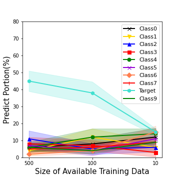
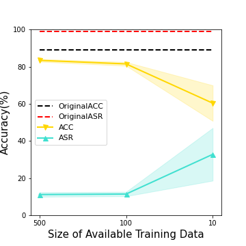
(a) The left shows the prediction portion for each class with perturbed neurons with various available training data size. The right shows the ASR/ACC of the ANP pruned models with various available training data size.

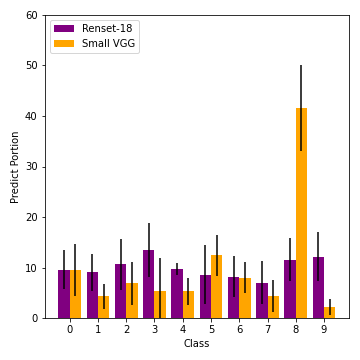
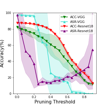
(b) The left shows the prediction portion for each class with perturbed neurons with ResNet and VGG model. The right shows the ASR/ACC of the ANP pruned models under various pruning threshold.

Figure 1: An illustrative example of the failure cases of ANP.

We then investigate how the network size affects ANP’s performance by applying it on both VGG (small) and ResNet-18 (large) backdoored models. The left part of Figure 1 (b) indicates that while ANP’s perturb neuron is able to show larger prediction portion on the target class, when applying on smaller VGG model, its magic failed again. The right part of Figure 1 (b) illustrates the ASR/ACC of the ANP pruned models under various pruning threshold. We can observe that it is hard to find a suitable pruning threshold for the smaller VGG network to obtain both high ASR and low ACC.

4 Our Proposed Method

In this section, we introduce our proposed method. Inspired by the above analysis in Section 3, we propose Adversarial Weight Masking (AWM) for better backdoor removal under practical settings.

Soft Weight Masking. From the analysis in Section 3, the neuron pruning method can be inappropriate when the backdoored model (with BN layers) is small and only has few layers: pruning certain neurons in the BN layer cuts off the information from a whole channel, which inevitably ignores some certain beneficial information for the clean tasks. To fix this drawbacks, we propose to adopt weight masking instead of neuron pruning. Let’s denote $\bm{\theta}\in\mathbb{R}^{d}$ as the entire neural network weights.

$$\min_{\mathbf{m}\in[0,1]^{d}}\mathbb{E}_{(\mathbf{x},y)\sim D}\ \alpha\mathcal{L}(f(\mathbf{x};\mathbf{m}\odot\bm{\theta}),y)+\beta\max_{\bm{\delta}\in[-\epsilon,\epsilon]^{d}}\mathcal{L}(f(\mathbf{x};(\mathbf{m}+\bm{\delta})\odot\bm{\theta}),y)$$ (4.1)

where $\bm{\delta}$ denotes the small perturbations on the network parameters, $\mathbf{m}$ is the weight mask of the same dimension as $\bm{\theta}$, $\odot$ denotes the Hadamard product (element-wise product). Eq. (4.1) follows the general idea of ANP by first identifying the sensitive part of the neural network and then lower such sensitivity. The major changes here is that we are no longer pruning out the neurons, instead, we add an additional mask for all the network weights. Note that such design would provide more flexibility in removing backdoor-related parts and thus avoid over-killing in BN layers. Since we apply weight masking instead of neuron pruning, we can also use soft mask $\mathbf{m}\in[0,1]^{d}$ instead of binary neuron masks as in ANP [57].

Adversarial Trigger Recovery. Another issue identified in Section 3 is that ANP performs poorly when the available training data size is small. And it seems that under such challenging conditions, perturbing the mask itself does not give clues to which part of the network is really sensitive to the backdoor triggers. Inspired from adversarial training literature [36], we can first optimize the following objective for adversarially estimating the worst-case trigger patterns:

$$\max_{\|\bm{\Delta}\|_{1}\leqslant\tau}\mathbb{E}_{(\mathbf{x},y)\sim D}\ \mathcal{L}(f(\mathbf{x}+\bm{\Delta};\bm{\theta}),y),$$ (4.2)

where $\|\cdot\|_{1}$ denotes the $L_{1}$ norm and $\tau$ limits the strength of the perturbation. Note that technically speaking, Eq. (4.2) only aims to find a $L_{1}$ norm universal perturbation that can mislead the current model toward misclassification. Yet since we are not aware of the target class, this is a reasonable surrogate task for the trigger recovery. Based on Eq. (4.2), we can integrate it with soft weight masking and formulate it as a min-max optimization problem:

$$\min_{\mathbf{m}\in[0,1]^{d}}\mathbb{E}_{(\mathbf{x},y)\sim D}\ \alpha\mathcal{L}(f(\mathbf{x};\mathbf{m}\odot\bm{\theta}),y)+\beta\max_{\|\bm{\Delta}\|_{1}\leqslant\tau}\left[\mathcal{L}(f(\mathbf{x}+\bm{\Delta};\mathbf{m}\odot\bm{\theta}),y)\right],$$ (4.3)

where $\alpha$ and $\beta$ are tunable hyper-parameters.

Sparsity Regularization. To push our defense to mask out backdoor-related weights more aggressively, we adopt the $L_{1}$ norm regularization on $\mathbf{m}$ for further controlling its sparsity level, as inspired by previous works [52, 49] on trigger optimization.

Combining soft weight masking, adversarial trigger recovery together with sparsity regularization on $\mathbf{m}$, gives the full Adversarial Weight Masking formulation:

$$\min_{\mathbf{m}\in[0,1]^{d}}\mathbb{E}_{(\mathbf{x},y)\sim D}\ \alpha\mathcal{L}(f(\mathbf{x};\mathbf{m}\odot\bm{\theta}),y)+\beta\max_{\|\bm{\Delta}\|_{1}\leqslant\tau}\left[\mathcal{L}(f(\mathbf{x}+\bm{\Delta};\mathbf{m}\odot\bm{\theta}),y)\right]+\gamma\|\mathbf{m}\|_{1},$$ (4.4)

where $\alpha$, $\beta$ and $\gamma$ are tunable hyper-parameters. Intuitively, AWM works by first identifying the worst-case universal triggers (which are highly likely to be the actual triggers or different patterns with similar backdoor effects), and then finding an optimal weight mask $\mathbf{m}$ to lower the importance on the identified triggers while maintaining the accuracy on clean tasks.

Unlike ANP, which directly prunes out the suspicious neurons, we aim at learning a soft mask for each parameter weight, i.e., each element in $\mathbf{m}$ lies in between $[0,1]$. Such design can help preserve the information beneficial to the clean tasks and thus avoid over-killing. Moreover, adopting soft masks can also avoid the problem of setting the hyper-parameters on the pruning threshold, which is also heuristic and hard to generalize for various experimental settings.

Algorithm 1 Adversarial Weight Masking (AWM)

Input: Infected DNN $f$ with $\bm{\theta}$, Clean dataset $D=\{(\mathbf{x}_{i},y_{i})\}_{i=1}^{n}$, Batch size $b$, Learning rate $\eta_{1},\eta_{2}$, Hyper-parameters $\alpha,\beta,\gamma$, Epochs $E$, Inner iteration loops $T$, $L_{1}$ norm bound $\tau$

1:  Initialize all elements in $\bf{m}$ as 1

2:  for $i=1$ to $E$ do

3:     Initialize $\bm{\Delta}$ as ${\bm{0}}$ // Phase 1: Inner Optimization

4:     for $t=1$ to $T$ do

5:        Sample a minibatch $(\mathbf{x},y)$ from $D$ with size $b$

6:        $\mathcal{L}_{inner}=\mathcal{L}(f(\mathbf{x}+\bm{\Delta};\mathbf{m}\odot\bm{\theta}),y)$

7:        $\bm{\Delta}=\bm{\Delta}-\eta_{1}\nabla_{\bm{\Delta}}\mathcal{L}_{inner}$

8:     end for

9:     Clip $\bm{\Delta}$: $\bm{\Delta}=\bm{\Delta}\times\min(1,\frac{\tau}{\|\bm{\Delta}\|_{1}})$ // Phase 2: Outer Optimization

10:     for $t=1$ to $T$ do

11:        $\mathcal{L}_{outer}=\alpha\mathcal{L}(f(\mathbf{x};\mathbf{m}\odot\bm{\theta}),y)+\beta\mathcal{L}(f(\mathbf{x}+\bm{\Delta};\mathbf{m}\odot\bm{\theta}),y)+\gamma\|\mathbf{m}\|_{1}$

12:        $\mathbf{m}=\mathbf{m}+\eta_{2}\nabla_{\mathbf{m}}\mathcal{L}_{outer}$

13:        Clip $\mathbf{m}$ to $[0,1]$.

14:     end for

15:  end for Output: Filter masks $\mathbf{m}$ for weights in network $f$.

Algorithm Details. The detailed steps of AWM is summarized in Algorithm 1. We solve the min-max optimization problem in Eq. (4.4) by alternatively solving the inner and outer objectives. Specifically, we initialize all the mask values as $1$. In each epoch, we repeat the following steps: 1) initialize $\bm{\Delta}$ as ${\bm{0}}$, and then perform $K$-steps of gradient descent on $\bm{\Delta}$ and clip it with its $L_{1}$ norm limit $\tau$; 2) we update soft weight mask in the outer optimization via stochastic gradient descent, where the first term is to minimize the clean classification loss, the second term is for lowering the weights associated with $\bm{\Delta}$, and the third term is the $L_{1}$ regularization on $\mathbf{m}$, followed by a clipping operation to keep $\mathbf{m}$ within $[0,1]$. Note that we reinitialize $\bm{\Delta}$ in each inner optimization as we need to relearn the adversarial perturbation based on the current $\mathbf{m}\odot\bm{\theta}$. We also on purposely set $T>1$ for ensuring sufficient optimization during each update in order to reach better convergence.

5 Experiments

In this section, we conduct thorough experiments to verify the effectiveness of our proposed AWM method and analyze the sensitivity on hyper-parameters via ablation studies.

Datasets and Networks. We conduct experiments on two datasets: CIFAR-10 [26] and GTSRB [20]. CIFAR-10 contains $50000$ training data and $10000$ test data of 10 classes. GTSRB is a dataset of traffic signal images, which contains $39209$ training data and $12630$ test data of 43 classes. The poisoned model is trained with full training data with $5\%$ poison rate on Resnet-18 [18], ShuffleNet V2 [34], MobileNet V2 [42], or a small VGG [46] network with three simplified blocks, containing six convolution layers followered by BN layers. See Appendix A for more experimental setting details and Appendix B for results on GTSRB.

Attacks and Defenses. For the backdoor attack baselines, we consider 1) BadNets with square trigger (BadNets) [15]; 2) Trojan-Watermark (WM) and Trojan-Square (SQ) [32]; 3) $l_{0}$-inv and $l_{2}$-inv [27], two invisible attack methods with different optimization constraints; 4) Blended attack (BLD) [6]; 5) Clean-label attack (CLB) [51]; 6) WaNet [38] with both single target and all-to-all (a2a) target settings. We mainly compare our method with two latest state-of-the-art methods of backdoor removal: Implicit Backdoor Adversarial Unlearning (IBAU) [60], Adversarial Neuron Pruning (ANP) [57].

Evaluations. We adopt two metrics: ACC and ASR. ACC is the test accuracy on clean dataset, while ASR is calculated as the ratio of those triggered samples that are still predicted as the adversary’s target labels. Note that usually a benign classifier is not assciated with a specific trigger, thus its prediction on poisoned data mainly follows its prediction on clean data. Under such case, suppose we have $c$ classes in total, we can expect the ASR should be around $1/c$, that is, $10\%$ for CIFAR-10 and $2.3\%$ for GTSRB. Therefore, once the backdoor removal method achieves an ASR close to $1/c$ (less than $1.5/c$), we consider it as successfully remove the backdoor (rather than achieving ASR$=0\%$).

5.1 Backdoor Removal with Various Available Data Size

Table 1: Backdoor removal performance comparison with various available data sizes on CIFAR-10 dataset with Resnet-18 and VGG Net. Numbers represent percentages. Bold numbers indicate the best ACC after backdoor removal and blue numbers indicate successful backdoor removal.

Attack	Available	Resnet-18							VGG Net
	Data Size	Origin	ANP		IBAU		AWM(Ours)		Origin	ANP		IBAU		AWM(Ours)
	n		ACC	ASR	ACC	ASR	ACC	ASR		ACC	ASR	ACC	ASR	ACC	ASR
BadNets	5000	ACC	85.56	10.18	86.41	11.26	86.94	10.46	ACC	77.34	8.64	81.06	12.25	83.58	13.98
	500	87.83	83.39	11.15	84.88	35.61	83.56	12.11	85.98	73.17	13.76	77.30	13.52	78.20	11.93
	200	ASR	83.52	11.53	82.38	83.89	84.26	10.90	ASR	64.59	13.35	75.88	14.75	76.42	12.82
	100	97.90	81.48	11.42	78.80	97.82	83.57	11.10	97.96	51.19	15.86	75.53	33.62	75.69	10.64
	50		81.09	11.21	73.84	98.92	80.46	11.42		49.81	17.66	68.72	45.23	73.20	12.22
Trojan-SQ	5000	ACC	87.30	10.66	86.34	9.38	87.08	11.21	ACC	67.70	8.68	82.38	14.20	83.82	12.76
	500	88.27	85.34	9.34	81.08	10.38	86.30	10.34	85.86	63.21	35.77	76.42	11.53	79.40	10.08
	200	ASR	82.72	10.51	75.72	99.94	85.38	9.41	ASR	63.84	36.31	73.81	10.69	75.50	14.40
	100	99.61	80.28	7.42	66.38	93.82	85.68	10.32	99.36	40.23	7.14	74.32	55.68	74.49	12.08
	50		69.68	9.29	39.83	98.80	80.78	8.48		40.06	6.41	73.20	84.32	72.23	5.01
Trojan-WM	5000	ACC	85.72	38.48	84.68	14.32	87.12	12.92	ACC	58.14	31.70	83.03	8.26	82.78	13.64
	500	88.00	82.82	34.06	80.63	10.22	85.17	8.36	86.08	55.64	9.76	82.89	7.33	82.61	12.15
	200	ASR	83.43	66.30	80.32	20.68	84.88	11.10	ASR	52.58	8.45	80.27	10.36	81.96	17.88
	100	99.96	75.99	61.64	78.75	38.82	83.31	12.51	99.80	42.95	21.20	81.02	30.25	81.56	12.82
	50		70.52	9.33	69.42	99.78	80.14	3.43		46.84	6.15	78.33	35.06	79.97	8.88
$l_{0}$ inv	5000	ACC	86.08	15.20	85.32	10.72	86.38	11.74	ACC	66.90	10.21	82.90	12.68	82.26	12.88
	500	88.23	83.71	15.08	80.83	14.48	84.97	11.81	86.56	67.70	30.20	80.42	10.11	75.01	20.54
	200	ASR	83.47	18.18	75.83	28.90	82.83	17.79	ASR	69.47	73.10	76.26	95.50	76.20	33.74
	100	100.0	77.32	16.44	73.49	70.18	82.04	12.68	100.0	60.31	59.14	67.40	93.56	62.31	24.58
	50		69.21	25.26	69.83	85.34	77.68	25.73		54.95	58.08	59.13	78.20	60.73	45.36
$l_{2}$ inv	5000	ACC	85.04	12.14	86.46	7.28	87.22	10.76	ACC	70.70	7.58	81.51	6.23	82.74	12.94
	500	88.51	82.25	31.99	78.66	9.32	85.76	10.26	86.22	74.80	0.44	78.09	7.64	81.33	4.39
	200	ASR	82.21	30.68	77.38	50.46	85.16	11.45	ASR	66.38	0.92	73.28	6.42	80.36	6.39
	100	99.86	81.80	21.68	73.26	90.48	82.26	8.85	99.84	53.07	1.12	72.91	18.86	81.67	7.55
	50		72.65	8.90	63.21	93.46	75.60	10.86		47.87	0.15	75.41	30.27	80.36	9.93

We first study the backdoor removal performances of AWM on various available data sizes and compare with other state-of-the-art defense baselines. Table 1 presents the defense results on the CIFAR-10 dataset. Specifically, among the entire CIFAR-10 training data, 2500 images are backdoored. We test with varying size of available data samples ranging from $5000$ to $10$ for each defense. A fixed number of $5000$ remaining samples are used to evaluate the defense result.

The left column depicts five single-target attack methods, and the first row represents two different adopted network structures. Note that each attack’s poison rates are set to be $5\%$. We present the ACC and ASR under each backdoor removal setting in the table. All single-target attacks are capable of achieving an ASR close to $100\%$ and an ACC around $88\%$ with no defenses. For Resnet-18, the performance of the baselines are comparable with AWM when there are sufficient available training data ($n=5000$): all methods effectively remove the backdoors. With the decreasing size of clean data, IBAU suffers from huge performance degradation and fails to remove the backdoor under several settings. The major reason is that its fine-tuning procedure can actually hurt the original information stored in the parameters that are crucial to its clean accuracy, especially when fine-tuning on small sample set. On the other hand, ANP shows better robustness as it prunes the neurons which reduces the negative effect of insufficient data, but still fails on more challenging cases. On the right part of Table 1, we can observe that ANP losses more accuracy on the small VGG network, which backup our analysis in Section 3. AWM shows state-of-the-art backdoor removal performances with various available data sizes, network structures and successfully erase the neuron backdoors in most cases.

Table 2: An Extreme Case: One-Shot Backdoor Removal Comparison on CIFAR-10 Data. Numbers represent percentages. Bold numbers indicate the best ACC after backdoor removal and blue numbers indicate successful backdoor removal.

Method	BadNets		Trojan-SQ		Trojan-WM		$l_{0}$ inv		$l_{2}$ inv
	ACC	ASR	ACC	ASR	ACC	ASR	ACC	ASR	ACC	ASR
Origin	87.83	97.90	88.27	99.61	88.00	99.96	88.23	100.0	88.51	99.86
ANP	60.35	32.83	68.32	13.88	50.42	35.50	63.42	22.46	67.08	76.16
IBAU	60.18	97.33	45.38	96.27	57.76	99.93	69.26	95.81	63.48	89.42
AWM (Ours)	76.46	8.98	78.26	10.68	74.28	8.66	69.94	10.18	76.60	10.64

We further conduct experiments in an extreme one-shot setting, i.e., we only provide one image per class as the available data for backdoor removal tasks (total size as 10 for CIFAR-10 dataset). Table 2 shows the result of ACC and ASR under such a one-shot setting. In this case, we randomly sample one image for each of the ten classes and use the basic data-augmentation method, such as random horizontal flip and random crop. As a result, our AWM successfully removes all those backdoors with minimal performance drop ($10\%$ higher than other baselines on average). In contrast, other baselines failed in removing the existing backdoor triggers for most cases (as suggested by the large ASR values).

5.2 Reliability of AWM under Different Attack Types and Network Architectures

Table 3: Backdoor removal performance comparison with lightweight architectures and universal or all-to-all attacks.

	ShuffleNet V2
	BLEND		CLB		WaNet		WaNet(a2a)
	ACC	ASR	ACC	ASR	ACC	ASR	ACC	ASR
No Defense	84.37	99.93	83.41	99.78	89.85	99.22	89.57	84.25
ANP	44.15	32.51	62.47	6.53	64.39	4.77	72.58	10.03
AWM	69.75	2.69	70.33	2.19	76.35	7.49	75.81	9.73
	MobileNet V2
No	88.83	99.78	87.70	100.0	93.78	91.01	94.08	92.72
ANP	51.95	85.33	57.65	22.09	75.31	18.97	79.28	10.33
AWM	67.87	2.10	66.68	9.70	74.29	8.92	80.97	13.38

To comprehensively show our performance on different network structures and attack types, we select two more lightweight networks and four more backdoor attacks to conduct experiments under the one-shot setting. We summarize the ACC and ASR on CIFAR-10 in Table 3.

Robustness on Network Architectures. Different from the VGG we adopted to illustrate "a small network", ShuffleNet and MobileNet contain more convolutional and BN layers while their parameters are fewer. Although the performance gap between ANP and AWM closes up a little bit, AWM still consistently cleans up all the backdoors with better clean task performances. This phenomenon also gives us insights that the performance of neuron pruning methods may be related to network depth more than the amount of parameters. To sum up, AWM works well on various structures of small neural networks with limited resources.

Robustness on Trigger Types. AWM accommodates different types of triggers as it does not make an assumption on the formulation of triggers. Although we used the adversarial trigger recovery and sparsity regularization as parts of techniques, they do not put a constraint on the triggers to be fixed or sparse but help remove the non-robust features in the poisoned network from the root.

The results on Blend, CLB, and WaNet also support the reasoning. The Blend attack uses gaussian noise (poison rate = $1\%$) that covers the whole image. We adopted the CLB attack with adversarial perturbations and triggers on four corners. WaNet warps the image with a determined warping field as poisoned data, so there does not exist a fixed trigger pattern. As it uses a noisy warping field to generate noisy data with actual labels, it is difficult to train a backdoored model with a poison rate of $1\%$. We set the poison rate as $10\%$. These three attacks cover scenarios that triggers are dynamic and natural. Thus the experimental results verify that AWM does not rely on universal and sparse triggers. The above-mentioned attacks are mostly all-to-one, except for the CLB. To fill the blank of all-to-all attacks, we perform all-to-all attacks with WaNet on CIFAR-10 and the all-to-all attack with Trojan-SQ pattern on GTSRB in Appendix B. In conclusion, AWM performs well on fixed, universal, dynamic triggers and all clean label, all-to-one, and all-to-all attack settings.

5.3 Ablation Study on Each Component of AWM

Table 4: The Effect of Each Component: From ANP to AWM. ${\color[rgb]{1,0,0}+}$ and ${\color[rgb]{0,0,1}-}$ indicate an increase or decrease in accuracy. $\downarrow$ indicates large improvements in lowering ASR. R denotes Resnet-18.

Attack$\&$Network	Avail.	ANP		ANP+SWM		ANP+SWM+ATR		Full AWM
	Data Size	ACC	ASR	ACC	ASR	ACC	ASR	ACC	ASR
BadNets (R)	500	83.39	11.15	83.25 (-0.14)	12.62	84.78 (+1.53)	12.08	85.33 (+0.55)	11.76
	100	81.48	11.42	82.25 (+0.77)	13.04	83.83 (+1.58)	9.55	83.57 (-0.26)	11.10
	10	53.26	34.38	73.34 (+19.9)	10.16 $\downarrow$	80.38 (+7.04)	10.41	76.46 (-3.92)	8.98
Trojan-SQ (R)	500	85.34	9.34	85.27 (-0.07)	12.00	84.06 (-1.19)	9.02	84.91 (-0.85)	10.20
	100	80.28	7.42	82.01 (+1.73)	10.35	83.23 (+1.22)	11.95	85.07 (+1.84)	11.34
	10	68.32	13.88	73.12 (+4.80)	11.42	82.04 (+8.92)	10.72	78.26 (-3.78)	10.68
Trojan-WM (R)	500	82.82	34.06	83.07 (+0.25)	9.34 $\downarrow$	85.23 (+2.16)	7.79	84.88 (-0.35)	10.12
	100	75.99	31.64	78.23 (+2.24)	15.02 $\downarrow$	82.99 (+4.76)	4.61 $\downarrow$	84.21 (+1.22)	11.18
	10	50.42	35.50	61.64 (+11.2)	17.88 $\downarrow$	75.66 (+14.0)	7.54 $\downarrow$	74.28 (-1.38)	8.66
$l_{0}$ inv (R)	500	83.71	15.08	83.31 (-0.40)	11.67	84.14 (+0.83)	13.91	84.83 (0.69)	12.15
	100	77.32	16.44	81.16 (+3.84)	13.11	84.39 (+3.23)	17.87	82.44 (+1.95)	11.97
	10	63.42	22.46	65.46 (+2.04)	10.40	73.66 (+8.20)	14.70	69.94 (+3.72)	10.18
$l_{2}$ inv (R)	500	82.25	31.99	82.59 (+0.34)	13.94 $\downarrow$	82.15 (-0.45)	6.26	85.22 (+3.07)	13.13
	100	81.80	21.68	80.51 (-1.29)	10.47 $\downarrow$	81.08 (+0.57)	11.24	79.79 (+1.29)	11.77
	10	67.08	76.16	60.36 (-6.72)	12.20 $\downarrow$	66.78 (+6.42)	15.80	76.60 (+9.82)	10.64
$l_{2}$ inv (VGG)	500	74.80	0.44	76.35 (+1.55)	3.17	82.08 (+5.73)	5.81	81.33 (-0.75)	4.39
	100	66.38	0.92	75.63 (+9.25)	7.89	79.42 (+3.79)	6.46	80.36 (+0.94)	6.39
	10	47.08	30.15	70.82 (+23.7)	19.17	78.34 (+7.52)	14.73	80.32 (+1.98)	12.52

We further perform an ablation study on each component of AWM. For notational simplicity, we refer the soft weight masking as SWM, and adversarial trigger recovery as ATR. From left to right in Table 4, we demonstrate the performance of the original ANP method, ANP + SWM (as in Eq. (4.1)), ANP + SWM + ATR (as in Eq. (4.3), and our full AWM method.

Table 4 shows that each component in AWM is non-trivial and necessary since adding each component would enhance the performance on average. Previous analysis in Section 3 suggests two of the ANP’s weaknesses: when the network is small and when the available training data size is small. The first weakness motivates us to adopt soft label masking. As expected, SWM contributes more with the small VGG net and verifies that it overcomes the drawback of neuron pruning in a smaller network’s BN layer. The second weakness motivates us to perform adversarial trigger recovery. From Table 4 we can easily observe ATR’s improvements in lowering the ASR and significantly improving the ACC. The effect of $L_{1}$ regularization is comparably small but indeed forces the mask $\mathbf{m}$ to be sparser and thus further lowering the influence of weights associated with the recovered trigger patterns.

5.4 Additional Ablation Studies

In this section, we perform additional empirical studies on the necessity of regularization and AWM’s robustness on the hyper-parameters. We compare our AWM with the following modified models: 1) No Clip: AWM with no $\bm{\Delta}$ clipping; 2) No Shrink: AWM with no $L_{1}$ regularization on $\mathbf{m}$; 3) NC-NS: AWM with no $\bm{\Delta}$ clipping and $\mathbf{m}$ regularization; 4) $L_{2}$ Reg: AWM with $\bm{\Delta}$’s $L_{2}$ regularization; 5) $L_{2}$ Reg NC: AWM with $\bm{\Delta}$’s $L_{2}$ regularization and no clipping;

Table 5: Ablation Study on AWM. $\downarrow$ indicates significant performance drop; $\uparrow$ indicates negative effect on backdoor removal. The base for comparison is Full AWM.

Avail.	Method	BadNets		Trojan-SQ		Trojan-WM		$l_{0}$ inv		$l_{2}$ inv
Data Size		ACC	ASR	ACC	ASR	ACC	ASR	ACC	ASR	ACC	ASR
200	No Clip	82.86 $\downarrow$	19.36 $\uparrow$	79.21 $\downarrow$	20.58 $\uparrow$	84.82	32.16 $\uparrow$	80.17 $\downarrow$	46.85 $\uparrow$	81.76 $\downarrow$	17.28 $\uparrow$
	No Shrink	84.52	10.31	83.06 $\downarrow$	9.20	84.33	9.96	83.34	16.52	84.66	10.43
	NC-NS	82.33 $\downarrow$	15.78 $\uparrow$	78.41 $\downarrow$	26.93 $\uparrow$	84.40	37.81 $\uparrow$	77.84 $\downarrow$	36.37 $\uparrow$	81.80 $\downarrow$	12.39
	$L_{2}$ Reg	81.46 $\downarrow$	13.29	83.60 $\downarrow$	8.81	83.93	14.63	83.04	18.52	85.30	9.48
	$L_{2}$ Reg NC	83.72	11.64	83.49 $\downarrow$	30.13 $\uparrow$	83.55 $\downarrow$	7.56	81.27 $\downarrow$	29.61 $\uparrow$	83.45 $\downarrow$	21.54 $\uparrow$
	Full AWM	84.26	10.90	85.38	9.41	84.88	11.10	82.83	17.79	85.16	11.44
one-shot	No Clip	66.03 $\downarrow$	16.28 $\uparrow$	62.14 $\downarrow$	20.68 $\uparrow$	55.32 $\downarrow$	12.28	61.68 $\downarrow$	37.38 $\uparrow$	72.71	16.15 $\uparrow$
	No Shrink	66.32 $\downarrow$	9.97	76.62	12.83	73.50	9.26	70.69	21.36 $\uparrow$	75.57	14.86
	NC NS	65.32 $\downarrow$	9.77	68.17 $\downarrow$	26.14 $\uparrow$	73.62	59.52 $\uparrow$	70.22	24.87 $\uparrow$	71.52	29.84 $\uparrow$
	$L_{2}$ Reg	72.71	8.98	75.21	8.06	71.32	8.48	72.42	14.73	76.96	12.35
	$L_{2}$ Reg NC	73.96	14.38	72.50 $\downarrow$	13.74	73.39	10.61	68.94	31.53 $\uparrow$	72.06	20.87 $\uparrow$
	Full AWM	76.46	8.98	78.26	10.68	74.28	8.66	69.94	10.18	76.60	10.64

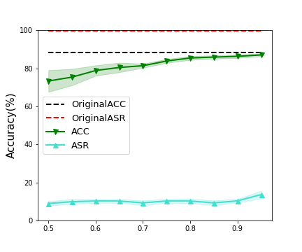
(a) Coefficient $\alpha$

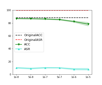
(b) Coefficient $\gamma$

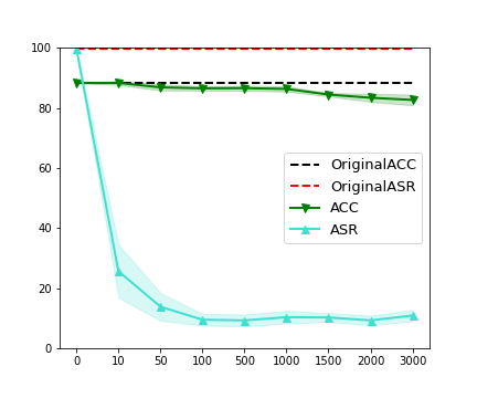
(c) Clipping bound $\tau$

Figure 2: Sensitivity on hyper-parameters. Performance ($\pm$std) over 5 random runs is reported.

Constraints on $\bm{\Delta}$ and $\mathbf{m}$. In Table 5, we compare the results of different modifications of AWM. On the one hand, the clipping of the virtual trigger $\bm{\Delta}$ is necessary as No Clip and $L_{2}$ Reg NC either remove the backdoor incompletely or sacrifice the accuracy too much. $L_{2}$ Reg changes the form of regularization and achieves comparable results on several settings but is less stable than AWM. The comparison between AWM and $L_{2}$ Reg also shows that both $L_{1}$ and $L_{2}$ norm regularization work for $\bm{\Delta}$. On the other hand, the regularization of $\mathbf{m}$ helps better learn the soft mask. NC-NS differs from No Clip only in the $\mathbf{m}$ but successfully unlearns more backdoors. This is also reasonable since: by punishing the $L_{1}$ norm, the soft masks are forced to reach smaller values and thus be more aggressive on suspicious trigger-related features.

Hyper-parameters. We first use one single defend task to test AWM’s sensitivity to hyper-parameters: the coefficient $\alpha$, $\gamma$, and the clipping bound $\tau$ for $\bm{\Delta}$. Concretely, $\alpha$ controls the trade-off between the clean accuracy and backdoor removal effect, $\gamma$ controls the sparsity of weight masks, and $\tau$ controls the maximum $L_{1}$ norm of the recovered trigger pattern. We test with $\alpha\in[0.5,0.8],\beta=1-\alpha,\gamma\in[10^{-8},10^{-5}],\tau\in[10,3000]$ and shows the performance changes under the Trojan-SQ attack with 500 training data. When varying the value of one specific hyper-parameter, we fix the others to the default value as $\alpha_{0}=0.9,\gamma_{0}=10^{-7},\tau_{0}=1000$. As shown in Figure 2, $\gamma$ is quite robust within the selected range. However, if we choose an overly large $\gamma$, the mask would shrink its value and hurt the accuracy. $\alpha$ works best around $0.8$ to $0.9$. If $\alpha$ is too close to $1$, the major goal of AWM will shift to maintain clean accuracy while paying less attention to backdoor removal. The clipping bound $\tau$ should also be selected within a moderate range, as the adversarial perturbation should neither be too small to fail in capturing the real trigger nor be too large to lead to difficulties in finding the optimal soft mask $\mathbf{m}$. In addition, considering the data dimension for CIFAR-10, further increasing $\tau$ after $3000$ is the same as no constraint and thus meaningless.

As observed, the impacts of $\alpha$ and $\gamma$ on the performance has a single decrease or increase, while the clipping bound $\tau$ needs a moderate value. To verify the difficulty of selecting $\tau$, we then conduct experiments to compare the $\tau$s from $10$ to $3000$ for four attacks, keeping $\alpha$ and $\gamma$ to be 0.9 and $10^{-7}$.

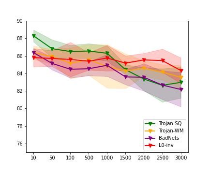
(a) ACC

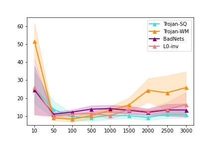
(b) ASR

Figure 3: Sensitivity on $\tau$ over different defend tasks. Performance ($\pm$std) over 5 random runs is reported.

Observing the ACC and ASR curves with Trojan-SQ, Trojan-WM, BadNets, and $L_{0}$-inv in Figure 3, the ACC decreases with the increase of $\tau$ while ASR first decreases fastly and then slightly increases again or keeps flat. The reasons behind this are easy to interpret. In terms of ACC, since we are using a larger $\tau$, the model weights are masked to adapt to triggered data points that are far different from the original data distribution. As a result, this will unavoidably hurt the original task ACC. On the other hand, in an ideal condition, ASR should decrease since the solution space of the optimization problem with larger $\tau$ actually contains the solution of the same problem with a smaller $\tau$. Thus in terms of backdoor removal, it should be at least as good as that of a smaller $\tau$. However, in practice, since we use PGD for solving the inner maximization problem, setting a large $\tau$ will simply make the $L_{1}$ norm of the recovered trigger too large. Thus the recovered trigger will be further away from the actual trigger and negatively affects the backdoor removal performances, especially on the variance.

Fortunately, the workable range of $\tau$ is indeed vast for various attacks, and it is pretty safe to select a value between $50$ and $1000$ for a $32\times 32$ image, which can be easily extended to other image sizes by the ratio $\tau/\text{image size}$. On the one hand, even if we falsely select an overly-large $\tau$, such as $3000$ for BadNets, the resulting ACC and ASR are still acceptable. On the other hand, we recommend selecting small $\tau$ because it tends to outperform the default setting. It is also reasonable to assume that the adversary tends to make a trigger invisible and small in the norm. For example, the $L_{1}$ norm of Trojan-WM’s actual trigger is around 115, which is way smaller than our default value of $\tau=1000$. In fact, $\tau=1000$ roughly means that we allow the trigger to significantly change the clean image over $16\times 16$ pixels in a $32\times 32$ image which has been fairly large.

6 Conclusions and Future Works

In this work, we propose a novel Adversarial Weight Masking method which adversarially recovers the potential trigger patterns and then lower the parameter weights associated to the recovered patterns. One major advantage of our method is its ability to consistently erasing neuron backdoors even in the extreme one-shot settings while the current state-of-the-art defenses cannot. Under scenarios with a few hundred clean data, AWM still outperforms other backdoor removal baselines. Extensive empirical studies show that AWM relies less on the network structure and the available data size than neuron pruning based methods.

Note that currently, our AWM method still needs at least one image per class in order to erase the neuron backdoors properly. In some cases, the defender may have no clue what the training data is. Under such settings, it would be wonderful if the model owner could also remove the backdoors in a data-free setting. In addition, it is still under-explored how the weight masks in different layers contribute to the results. It would also be interesting to explore whether an attacker could break the backdoor defense method with the knowledge of the optimization details. We leave these problems as future works.

Appendix A Additional Experimental Settings

VGG Network. In this work, we follow [60] to adopt a small VGG network with the following structure. Each convolution layer is followed by a BatchNorm layer and the activation function is ELU with $\alpha=1.0$. When using our AWM method, we need to substitute the Conv2d with MaskedConv2d.

	Input ($32\times 32\times 3$)
Block 1	Conv2d (MaskedConv2d) $3\times 3$, 32
	Conv2d (MaskedConv2d) $3\times 3$, 32
	Max Pooling $2\times 2$, 32
	Dropout (0.3)
Block 2	Conv2d (MaskedConv2d) $3\times 3$, 64
	Conv2d (MaskedConv2d) $3\times 3$, 64
	Max Pooling $2\times 2$, 64
	Dropout (0.4)
Block 3	Conv2d (MaskedConv2d) $3\times 3$, 128
	Conv2d (MaskedConv2d) $3\times 3$, 128
	Max Pooling $2\times 2$, 128
	Dropout (0.4)
	FC(2048)
	Softmax(Num of Classes)

Table 6: Structure of the small VGG network

Implementation. We adopt PyTorch [39] as the deep learning framework for implementations. In implementation, the outer optimization is conducted with Adam with a learning rate of 0.01 (decay to 0.001 after 50 epochs) and the inner optimization is conducted with SGD with a learning rate of 10. We use the default hyper-parameter setting as $\alpha=0.9,\beta=0.1,\gamma=10^{-8},\tau=1000$ for both CIFAR-10 and GTSRB datasets. The batch size for training is summarized in Table 7.

Available Data Size $n$	One-Shot	100	200	500	5000
Batch Size $b$	16	32	32	128	128

Table 7: Summary of the Batch Size Settings

Attack Setting. In the single-target attack setting, we set Class $8$ as the target for BadNets, Class $2$ as the target for Trojan-SQ and Trojan-WM, and Class $0$ as the target for $l_{0}$-inv, $l_{2}$-inv, BLEND, and WaNet. In the multi-target attack setting, we use the pattern of Trojan-SQ and relabel each sample from Class $n$ to $n+1$.

Appendix B Results on GTSRB

Table 8 presents the defense results on the GTSRB dataset. GTSRB dataset has $39209$ training data and $12630$ test data of 43 classes. Specifically, among the entire GTSRB training data, 1960 images are backdoored. We test with varying size of available data samples ranging from $5000$ to $43$ (one-shot) for each defense. The remaining samples are used to evaluate the defense result.

The left column depicts five single-target attack methods and one multi-target attack method. The first row represents two different adopted network structure. We present the ACC and ASR under each backdoor removal setting in the table, all attacks are capable of achieving an ASR close to $99\%$ and an ACC around $98\%$ with no defenses.

The performance of the baselines are comparable with AWM when there are sufficient available training data ($n=5000$): most methods effectively remove the backdoors. Similar to CIFAR-10, IBAU suffers from the biggest performance drop (higher ASR or fail to remove the backdoor). As the number of samples of Class $0$ is smaller than Class $2$ in GTSRB, it is much easier to remove the backdoor of $l_{0}$-inv and $l_{2}$-inv and achieve a very low ASR. However, in other attack settings, we can still observe that ANP is negatively affected by insufficient data. On the left part of Table 8, we can observe that ANP performs worse on the small VGG network, which backup our analysis in the paper. AWM shows state-of-the-art backdoor removal performances overall in this table.

As there are more classes in GTSRB than CIFAR-10, more instances are available in the one-shot setting, we do not use any data augmentation. Our AWM successfully removes all those backdoors while other baselines failed in removing the existing backdoor triggers for certain cases.

Table 8: Backdoor removal performance comparison with various available data sizes on GTSRB dataset with VGG and Resnet-18. Numbers represent percentages. Bold numbers indicate the best ACC after backdoor removal and blue color indicates successful backdoor removal.

Attack	Available	VGG							Resnet-18
	Data Size	Origin	ANP		IBAU		AWM(Ours)		Origin	ANP		IBAU		AWM(Ours)
	n		ACC	ASR	ACC	ASR	ACC	ASR		ACC	ASR	ACC	ASR	ACC	ASR
BadNets	5000	ACC	98.06	5.17	99.06	0.37	97.32	4.35	ACC	99.02	3.56	99.23	3.47	99.33	3.53
	500	98.11	97.35	6.35	97.02	0.32	98.90	4.31	98.58	98.47	3.40	98.65	3.91	96.50	3.25
	100	ASR	96.41	6.84	92.41	59.74	94.58	6.58	ASR	97.57	3.40	94.76	3.45	97.19	3.78
	One-shot	98.37	95.78	16.53	90.84	83.57	95.48	4.54	98.98	96.79	2.96	79.98	7.53	96.91	3.67
Trojan-SQ	5000	ACC	97.90	7.11	99.17	6.66	99.03	6.03	ACC	98.29	11.09	99.21	5.83	99.45	5.16
	500	98.18	97.49	11.49	96.82	5.92	98.17	7.05	98.83	98.55	8.64	98.81	5.77	96.58	6.18
	100	ASR	96.94	32.50	84.09	88.57	95.89	6.30	ASR	97.23	8.03	96.74	98.39	97.34	5.90
	One-shot	99.55	97.21	37.09	83.76	91.02	93.96	6.25	99.74	97.62	14.21	69.62	97.80	96.51	7.05
Trojan-WM	5000	ACC	98.03	7.20	99.02	0.53	99.25	5.70	ACC	98.39	3.66	99.11	6.41	99.15	4.79
	500	97.90	97.35	6.98	97.80	4.35	98.52	5.93	98.75	98.39	9.73	98.49	72.12	96.57	5.08
	100	ASR	97.13	19.65	90.37	15.84	94.38	5.06	ASR	97.89	9.87	96.38	94.94	96.86	7.89
	One-shot	99.82	97.45	25.49	88.65	30.52	93.74	5.99	99.65	97.71	46.52	87.27	93.41	96.15	6.74
$L_{0}$-inv	5000	ACC	98.07	0.48	99.27	0.46	98.73	0.35	ACC	98.85	0.64	99.26	0.83	99.45	0.42
	500	98.35	98.24	0.49	96.80	1.36	97.57	1.25	98.64	98.70	0.45	98.32	0.52	96.49	0.29
	100	ASR	97.72	0.38	84.24	7.14	94.05	0.96	ASR	97.63	0.58	96.68	38.09	93.73	0.22
	One-shot	100.0	97.51	0.43	80.71	10.63	94.56	0.73	100.0	97.56	0.48	83.66	58.11	93.25	0.32
$L_{2}$-inv	5000	ACC	97.79	6.74	99.13	0.54	98.98	1.81	ACC	98.65	1.27	98.87	0.43	99.46	0.46
	500	98.31	97.74	6.53	94.83	0.56	97.88	1.59	98.51	98.72	1.61	98.57	0.43	98.86	0.45
	100	ASR	97.21	0.46	88.45	7.03	96.36	6.17	ASR	97.95	6.26	91.22	0.00	97.63	0.44
	One-shot	99.80	97.21	0.74	87.42	6.89	96.09	2.37	99.93	97.35	6.67	88.00	42.53	96.78	0.61
all-to-all	5000	ACC	97.34	3.53	98.95	0.74	98.68	1.47	ACC	98.81	2.49	99.30	0.18	99.18	0.13
	500	98.15	95.70	3.03	96.45	10.74	98.02	4.45	98.59	98.50	2.32	97.79	4.78	96.22	0.65
	100	ASR	94.34	13.27	90.69	41.61	95.15	5.38	ASR	97.19	9.48	94.80	79.63	89.04	3.16
	One-shot	93.17	95.76	24.99	75.24	31.72	93.02	7.18	96.88	97.61	17.71	88.91	72.42	87.33	4.51

Convergence. Figure 4 demonstrates the one-shot training records of ACC and ASR in each epoch of AWM over the 5 single-target attacks. Note that we take ten steps of outer optimization after every 10 steps of inner optimization in each epoch. The backdoors are removed very quickly in most cases. Since we only have extremely insufficient clean data, it causes a little accuracy degradation after a long time of training. We report the averaged ACC and ASR after 100 epochs(1000 iterations) over 5 runs in previous table.

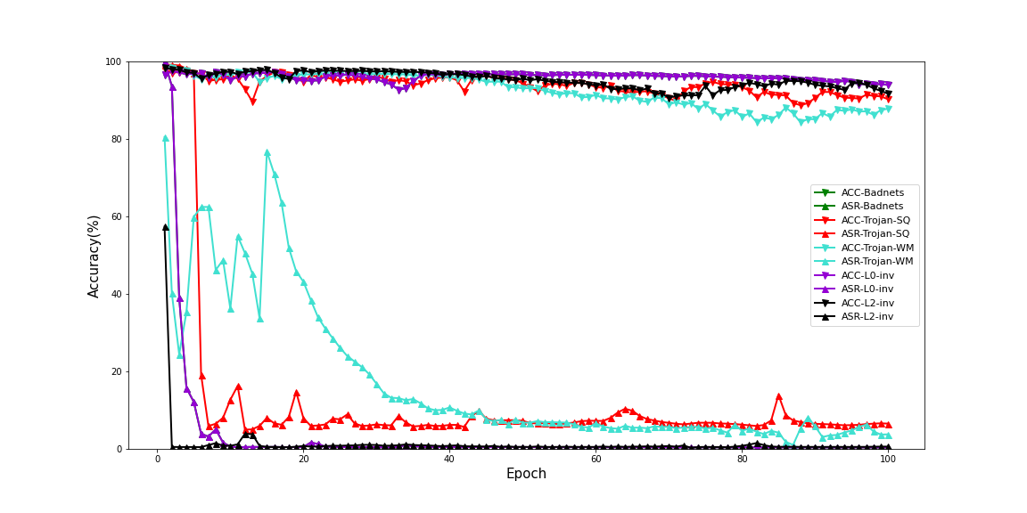
Figure 4: Training records of GTSRB (one-shot).

Appendix C Additional Studies of AWM

Masking Selected Layers. For the all-to-all attack on GTSRB, we visualize the distribution of mask values in different layers and try to achieve similar performance with masking fewer layers. Figure 5 shows the percentage of mask values falling into each interval. Most values fall in the smallest and the largest intervals, indicating the effect of sparsity constraint.

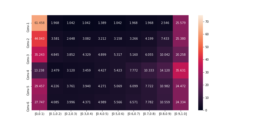
Figure 5: Distribution ($\%$) of weight mask values of VGG.

In the following experiment, we optimize the mask on each layer on CIFAR-10 with VGG. As shown in the Table 6, there are six convolution layers in this small VGG network. We name VGG-i as the VGG with only mask on the $i$-th convolution layer. We summarize the backdoor removal result with $100$ instances in Table 9. Masking shallow convolution layers, such as VGG-1, 2, and 3, is much easier to remove the backdoor comparing with masking deep layers. Another phenomenon is that masking the first convolution layer causes the largest loss on accuracy. This inspires that it might be possible to save the number of masks by limiting them in shallow layers.

Network	Number of Kernels	ACC	ASR
VGG	448	95.15	5.38
VGG-1	32	93.75	3.34
VGG-2	32	96.27	7.25
VGG-3	64	96.54	9.60
VGG-4	64	96.98	23.71
VGG-5	128	97.65	47.83
VGG-6	128	97.37	60.19

Table 9: Performance with Different Layers of Mask

We also visualizes the distribution of weight mask values in Figure 6. Note that this heatmap summarizes the six experiments and each row corresponds to the mask values in the specific layer. Figure 6 is similar to Figure 5: Overall, it shows that optimizing masks on a certain layer is dependent to other layers to some degree. Therefore, it is reasonable to consider separating or selectively optimizing masks on some layers, which we leave as future work.

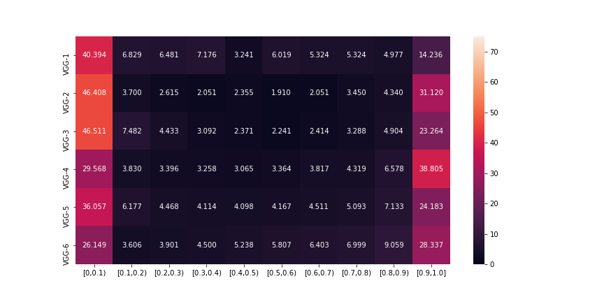
Figure 6: Distribution ($\%$) of weight mask values via masking different positions.

Defend Against Multiple Triggers. It is interesting to explore how to break a backdoor defense method with knowledge of how it works. Some principles in developing backdoor attacks, such as making triggers invisible or natural, are data-driven and do not direct a specific backdoor removal optimization procedure. The corresponding adaptive attack can potentially be complex on the device since the current backdoor removal techniques, including our AWM, have already involved complicated bi-level optimization.

As an attempt, we design a simple method targeting our backdoor trigger reconstruction mechanism: we only estimate one universal trigger $\Delta$ in every iteration. Now suppose the attacker knows our design and decides to inject multiple backdoor patterns into the model. They would hope our design could only remove one of them and thus fail on the other triggers.

The following table summarizes the result of defending against multiple backdoor triggers on CIFAR-10. We first train a poisoned model using three triggers: BadNets, Trojan-WM, and $L_{2}$-inv. The overall poison rate is set as $5\%$. Then we apply our AWM to remove the backdoors. ASR (all) represents the attack success rate as long as any one of the three triggers fooled the model. ASR1, ASR2, and ASR3 represent the attack success rate of each of the three triggers. Finally, ACC is the test accuracy on the clean test set. The results show that adding multiple triggers still cannot penetrate our AWM defense even with limited resources.

ShuffleNet	ASR(all)	ASR1	ASR2	ASR3	ACC
Original	99.83	95.80	99.52	99.15	84.86
AWM(500 images)	10.38	9.54	8.19	13.16	77.02
AWM(one-shot)	8.47	13.54	10.34	16.21	71.83

Table 10: Defend against multiple backdoors.

We conjecture that this is because although multiple triggers are involved, our algorithm will still try to identify the most likely triggers in each iteration. Thus when the first (the most prominent) ‘trigger’ is removed, the algorithm will automatically target the next likely ‘trigger’.

Such backdoor removal strategies seem to be hard to penetrate. Successful attacks may need to leverage tri-level optimization problems, which are notoriously hard to solve, or aim to make the removal strategy impractical by lowering its natural accuracy, which currently has no concrete solutions. We also leave this problem as one of our future work directions.

Appendix D Objectives in Ablation Study

We list the formal objective functions for the five modifications of AWM compared with in Section 5.3 of our paper.

0) Full AWM

$$\min_{\mathbf{m}\in[0,1]^{d}}\mathbb{E}_{(\mathbf{x},y)\sim D}\ \alpha\mathcal{L}(f(\mathbf{x};\mathbf{m}\odot\bm{\theta}),y)+\beta\max_{\|\bm{\Delta}\|_{1}\leqslant\tau}\left[\mathcal{L}(f(\mathbf{x}+\bm{\Delta};\mathbf{m}\odot\bm{\theta}),y)\right]+\gamma\|\mathbf{m}\|_{1},$$ (D.1)

1) No Clip: AWM with no $\bm{\Delta}$ clipping:

$$\min_{\mathbf{m}\in[0,1]^{d}}\mathbb{E}_{(\mathbf{x},y)\sim D}\ \alpha\mathcal{L}(f(\mathbf{x};\mathbf{m}\odot\bm{\theta}),y)+\beta\max\left[\mathcal{L}(f(\mathbf{x}+\bm{\Delta};\mathbf{m}\odot\bm{\theta}),y)\right]+\gamma\|\mathbf{m}\|_{1},$$ (D.2)

where $\beta$ is set to be $1-\alpha$.

2) No Shrink: AWM with no $L_{1}$ regularization on $\mathbf{m}$;

$$\min_{\mathbf{m}\in[0,1]^{d}}\mathbb{E}_{(\mathbf{x},y)\sim D}\ \alpha\mathcal{L}(f(\mathbf{x};\mathbf{m}\odot\bm{\theta}),y)+\beta\max_{\|\bm{\Delta}\|_{1}\leqslant\tau}\left[\mathcal{L}(f(\mathbf{x}+\bm{\Delta};\mathbf{m}\odot\bm{\theta}),y)\right].$$ (D.3)

3) NC-NS: AWM with no $\bm{\Delta}$ clipping and $\mathbf{m}$ regularization;

$$\min_{\mathbf{m}\in[0,1]^{d}}\mathbb{E}_{(\mathbf{x},y)\sim D}\ \alpha\mathcal{L}(f(\mathbf{x};\mathbf{m}\odot\bm{\theta}),y)+\beta\max\left[\mathcal{L}(f(\mathbf{x}+\bm{\Delta};\mathbf{m}\odot\bm{\theta}),y)\right].$$ (D.4)

4) $L_{2}$ Reg: AWM with $\bm{\Delta}$’s $L_{2}$ regularization;

$$\min_{\mathbf{m}\in[0,1]^{d}}\mathbb{E}_{(\mathbf{x},y)\sim D}\ \alpha\mathcal{L}(f(\mathbf{x};\mathbf{m}\odot\bm{\theta}),y)+\beta\max_{\|\bm{\Delta}\|_{2}\leqslant\tau}\left[\mathcal{L}(f(\mathbf{x}+\bm{\Delta};\mathbf{m}\odot\bm{\theta}),y)\right]+\gamma\|\mathbf{m}\|_{1}.$$ (D.5)

5) $L_{2}$ Reg NC: AWM with $\bm{\Delta}$’s $L_{2}$ regularization and no clipping;

$$\min_{\mathbf{m}\in[0,1]^{d}}\mathbb{E}_{(\mathbf{x},y)\sim D}\ \alpha\mathcal{L}(f(\mathbf{x};\mathbf{m}\odot\bm{\theta}),y)+\beta\max\left[\mathcal{L}(f(\mathbf{x}+\bm{\Delta};\mathbf{m}\odot\bm{\theta}),y)+\|\bm{\Delta}\|_{2}\right]+\gamma\|\mathbf{m}\|_{1}.$$ (D.6)

References

- [1] Mauro Barni, Kassem Kallas, and Benedetta Tondi. A new backdoor attack in cnns by training set corruption without label poisoning. In 2019 IEEE International Conference on Image Processing (ICIP), pages 101–105. IEEE, 2019.
- [2] Tom Brown, Benjamin Mann, Nick Ryder, Melanie Subbiah, Jared D Kaplan, Prafulla Dhariwal, Arvind Neelakantan, Pranav Shyam, Girish Sastry, Amanda Askell, et al. Language models are few-shot learners. Advances in neural information processing systems, 33:1877–1901, 2020.
- [3] Jinghui Chen, Yu Cheng, Zhe Gan, Quanquan Gu, and Jingjing Liu. Efficient robust training via backward smoothing. In Proceedings of the AAAI Conference on Artificial Intelligence (AAAI), 2022.
- [4] Jinghui Chen and Quanquan Gu. Rays: A ray searching method for hard-label adversarial attack. In Proceedings of the 26th ACM SIGKDD International Conference on Knowledge Discovery & Data Mining, pages 1739–1747, 2020.
- [5] Jinghui Chen, Dongruo Zhou, Jinfeng Yi, and Quanquan Gu. A frank-wolfe framework for efficient and effective adversarial attacks. In Proceedings of the AAAI Conference on Artificial Intelligence, 2020.
- [6] Xinyun Chen, Chang Liu, Bo Li, Kimberly Lu, and Dawn Song. Targeted backdoor attacks on deep learning systems using data poisoning. arXiv preprint arXiv:1712.05526, 2017.
- [7] Xinyun Chen, Wenxiao Wang, Chris Bender, Yiming Ding, Ruoxi Jia, Bo Li, and Dawn Song. Refit: a unified watermark removal framework for deep learning systems with limited data. In Proceedings of the 2021 ACM Asia Conference on Computer and Communications Security, pages 321–335, 2021.
- [8] Francesco Croce and Matthias Hein. Reliable evaluation of adversarial robustness with an ensemble of diverse parameter-free attacks. In International conference on machine learning, pages 2206–2216. PMLR, 2020.
- [9] Jacob Devlin, Ming-Wei Chang, Kenton Lee, and Kristina Toutanova. Bert: Pre-training of deep bidirectional transformers for language understanding. arXiv preprint arXiv:1810.04805, 2018.
- [10] Ilias Diakonikolas, Gautam Kamath, Daniel Kane, Jerry Li, Jacob Steinhardt, and Alistair Stewart. Sever: A robust meta-algorithm for stochastic optimization. In International Conference on Machine Learning, pages 1596–1606. PMLR, 2019.
- [11] Ji Feng, Qi-Zhi Cai, and Zhi-Hua Zhou. Learning to confuse: generating training time adversarial data with auto-encoder. Advances in Neural Information Processing Systems, 32, 2019.
- [12] Chao Gao, Yuan Yao, and Weizhi Zhu. Generative adversarial nets for robust scatter estimation: A proper scoring rule perspective. J. Mach. Learn. Res., 21:160–1, 2020.
- [13] Ian J Goodfellow, Jonathon Shlens, and Christian Szegedy. Explaining and harnessing adversarial examples. arXiv preprint arXiv:1412.6572, 2014.
- [14] Jianping Gou, Baosheng Yu, Stephen J Maybank, and Dacheng Tao. Knowledge distillation: A survey. International Journal of Computer Vision, 129(6):1789–1819, 2021.
- [15] Tianyu Gu, Brendan Dolan-Gavitt, and Siddharth Garg. Badnets: Identifying vulnerabilities in the machine learning model supply chain. arXiv preprint arXiv:1708.06733, 2017.
- [16] Wenbo Guo, Lun Wang, Xinyu Xing, Min Du, and Dawn Song. Tabor: A highly accurate approach to inspecting and restoring trojan backdoors in ai systems. arXiv preprint arXiv:1908.01763, 2019.
- [17] Kaiming He, Xiangyu Zhang, Shaoqing Ren, and Jian Sun. Deep residual learning for image recognition. In Proceedings of the IEEE conference on computer vision and pattern recognition, pages 770–778, 2016.
- [18] Kaiming He, Xiangyu Zhang, Shaoqing Ren, and Jian Sun. Deep residual learning for image recognition. In Proceedings of the IEEE conference on computer vision and pattern recognition, pages 770–778, 2016.
- [19] Geoffrey Hinton, Li Deng, Dong Yu, George E Dahl, Abdel-rahman Mohamed, Navdeep Jaitly, Andrew Senior, Vincent Vanhoucke, Patrick Nguyen, Tara N Sainath, et al. Deep neural networks for acoustic modeling in speech recognition: The shared views of four research groups. IEEE Signal processing magazine, 29(6):82–97, 2012.
- [20] Sebastian Houben, Johannes Stallkamp, Jan Salmen, Marc Schlipsing, and Christian Igel. Detection of traffic signs in real-world images: The german traffic sign detection benchmark. In The 2013 international joint conference on neural networks (IJCNN), pages 1–8. Ieee, 2013.
- [21] W Ronny Huang, Jonas Geiping, Liam Fowl, Gavin Taylor, and Tom Goldstein. Metapoison: Practical general-purpose clean-label data poisoning. Advances in Neural Information Processing Systems, 33:12080–12091, 2020.
- [22] Andrew Ilyas, Logan Engstrom, Anish Athalye, and Jessy Lin. Black-box adversarial attacks with limited queries and information. In International Conference on Machine Learning, pages 2137–2146. PMLR, 2018.
- [23] Andrew Ilyas, Shibani Santurkar, Dimitris Tsipras, Logan Engstrom, Brandon Tran, and Aleksander Madry. Adversarial examples are not bugs, they are features. Advances in neural information processing systems, 32, 2019.
- [24] Sergey Ioffe and Christian Szegedy. Batch normalization: Accelerating deep network training by reducing internal covariate shift. In International conference on machine learning, pages 448–456. PMLR, 2015.
- [25] Jinyuan Jia, Xiaoyu Cao, and Neil Zhenqiang Gong. Certified robustness of nearest neighbors against data poisoning attacks. arXiv preprint arXiv:2012.03765, 2020.
- [26] Alex Krizhevsky, Geoffrey Hinton, et al. Learning multiple layers of features from tiny images. 2009.
- [27] Shaofeng Li, Benjamin Zi Hao Zhao, Jiahao Yu, Minhui Xue, Dali Kaafar, and Haojin Zhu. Invisible backdoor attacks against deep neural networks. arXiv preprint arXiv:1909.02742, 2019.
- [28] Yige Li, Xixiang Lyu, Nodens Koren, Lingjuan Lyu, Bo Li, and Xingjun Ma. Neural attention distillation: Erasing backdoor triggers from deep neural networks. In International Conference on Learning Representations, 2020.
- [29] Yuezun Li, Yiming Li, Baoyuan Wu, Longkang Li, Ran He, and Siwei Lyu. Invisible backdoor attack with sample-specific triggers. In Proceedings of the IEEE/CVF International Conference on Computer Vision, pages 16463–16472, 2021.
- [30] Junyu Lin, Lei Xu, Yingqi Liu, and Xiangyu Zhang. Composite backdoor attack for deep neural network by mixing existing benign features. In Proceedings of the 2020 ACM SIGSAC Conference on Computer and Communications Security, pages 113–131, 2020.
- [31] Kang Liu, Brendan Dolan-Gavitt, and Siddharth Garg. Fine-pruning: Defending against backdooring attacks on deep neural networks. In International Symposium on Research in Attacks, Intrusions, and Defenses, pages 273–294. Springer, 2018.
- [32] Yingqi Liu, Shiqing Ma, Yousra Aafer, Wen-Chuan Lee, Juan Zhai, Weihang Wang, and Xiangyu Zhang. Trojaning attack on neural networks. In 25th Annual Network and Distributed System Security Symposium, NDSS 2018, San Diego, California, USA, February 18-221, 2018. The Internet Society, 2018.
- [33] Yunfei Liu, Xingjun Ma, James Bailey, and Feng Lu. Reflection backdoor: A natural backdoor attack on deep neural networks. In European Conference on Computer Vision, pages 182–199. Springer, 2020.
- [34] Ningning Ma, Xiangyu Zhang, Hai-Tao Zheng, and Jian Sun. Shufflenet v2: Practical guidelines for efficient cnn architecture design. In Proceedings of the European conference on computer vision (ECCV), pages 116–131, 2018.
- [35] Shiqing Ma and Yingqi Liu. Nic: Detecting adversarial samples with neural network invariant checking. In Proceedings of the 26th network and distributed system security symposium (NDSS 2019), 2019.
- [36] Aleksander Madry, Aleksandar Makelov, Ludwig Schmidt, Dimitris Tsipras, and Adrian Vladu. Towards deep learning models resistant to adversarial attacks. In International Conference on Learning Representations, 2018.
- [37] Tuan Anh Nguyen and Anh Tran. Input-aware dynamic backdoor attack. Advances in Neural Information Processing Systems, 33:3454–3464, 2020.
- [38] Tuan Anh Nguyen and Anh Tuan Tran. Wanet - imperceptible warping-based backdoor attack. In International Conference on Learning Representations, 2021.
- [39] Adam Paszke, Sam Gross, Francisco Massa, Adam Lerer, James Bradbury, Gregory Chanan, Trevor Killeen, Zeming Lin, Natalia Gimelshein, Luca Antiga, et al. Pytorch: An imperative style, high-performance deep learning library. Advances in neural information processing systems, 32, 2019.
- [40] Weiqi Peng and Jinghui Chen. Learnability lock: Authorized learnability control through adversarial invertible transformations. In International Conference on Learning Representations, 2022.
- [41] Han Qiu, Yi Zeng, Shangwei Guo, Tianwei Zhang, Meikang Qiu, and Bhavani Thuraisingham. Deepsweep: An evaluation framework for mitigating dnn backdoor attacks using data augmentation. In Proceedings of the 2021 ACM Asia Conference on Computer and Communications Security, pages 363–377, 2021.
- [42] Mark Sandler, Andrew Howard, Menglong Zhu, Andrey Zhmoginov, and Liang-Chieh Chen. Mobilenetv2: Inverted residuals and linear bottlenecks. In The IEEE Conference on Computer Vision and Pattern Recognition (CVPR), June 2018.
- [43] Ali Shafahi, W Ronny Huang, Mahyar Najibi, Octavian Suciu, Christoph Studer, Tudor Dumitras, and Tom Goldstein. Poison frogs! targeted clean-label poisoning attacks on neural networks. Advances in neural information processing systems, 31, 2018.
- [44] Ali Shafahi, Mahyar Najibi, Mohammad Amin Ghiasi, Zheng Xu, John Dickerson, Christoph Studer, Larry S Davis, Gavin Taylor, and Tom Goldstein. Adversarial training for free! Advances in Neural Information Processing Systems, 32, 2019.
- [45] Reza Shokri et al. Bypassing backdoor detection algorithms in deep learning. In 2020 IEEE European Symposium on Security and Privacy (EuroS&P), pages 175–183. IEEE, 2020.
- [46] Karen Simonyan and Andrew Zisserman. Very deep convolutional networks for large-scale image recognition. arXiv preprint arXiv:1409.1556, 2014.
- [47] Jacob Steinhardt, Pang Wei W Koh, and Percy S Liang. Certified defenses for data poisoning attacks. Advances in neural information processing systems, 30, 2017.
- [48] Christian Szegedy, Alexander Toshev, and Dumitru Erhan. Deep neural networks for object detection. Advances in neural information processing systems, 26, 2013.
- [49] Guanhong Tao, Guangyu Shen, Yingqi Liu, Shengwei An, Qiuling Xu, Shiqing Ma, Pan Li, and Xiangyu Zhang. Better trigger inversion optimization in backdoor scanning. In Proceedings of the IEEE/CVF Conference on Computer Vision and Pattern Recognition, pages 13368–13378, 2022.
- [50] Florian Tramèr, Alexey Kurakin, Nicolas Papernot, Ian Goodfellow, Dan Boneh, and Patrick McDaniel. Ensemble adversarial training: Attacks and defenses. arXiv preprint arXiv:1705.07204, 2017.
- [51] Alexander Turner, Dimitris Tsipras, and Aleksander Madry. Label-consistent backdoor attacks. arXiv preprint arXiv:1912.02771, 2019.
- [52] Bolun Wang, Yuanshun Yao, Shawn Shan, Huiying Li, Bimal Viswanath, Haitao Zheng, and Ben Y Zhao. Neural cleanse: Identifying and mitigating backdoor attacks in neural networks. In 2019 IEEE Symposium on Security and Privacy (SP), pages 707–723. IEEE, 2019.
- [53] Ren Wang, Gaoyuan Zhang, Sijia Liu, Pin-Yu Chen, Jinjun Xiong, and Meng Wang. Practical detection of trojan neural networks: Data-limited and data-free cases. In European Conference on Computer Vision, pages 222–238. Springer, 2020.
- [54] Maurice Weber, Xiaojun Xu, Bojan Karlaš, Ce Zhang, and Bo Li. Rab: Provable robustness against backdoor attacks. arXiv preprint arXiv:2003.08904, 2020.
- [55] Eric Wong, Leslie Rice, and J. Zico Kolter. Fast is better than free: Revisiting adversarial training. In International Conference on Learning Representations, 2020.
- [56] Boxi Wu, Jinghui Chen, Deng Cai, Xiaofei He, and Quanquan Gu. Do wider neural networks really help adversarial robustness? Advances in Neural Information Processing Systems, 34, 2021.
- [57] Dongxian Wu and Yisen Wang. Adversarial neuron pruning purifies backdoored deep models. Advances in Neural Information Processing Systems, 34, 2021.
- [58] Kaidi Xu, Sijia Liu, Pin-Yu Chen, Pu Zhao, and Xue Lin. Defending against backdoor attack on deep neural networks. arXiv preprint arXiv:2002.12162, 2020.
- [59] Xiaojun Xu, Qi Wang, Huichen Li, Nikita Borisov, Carl A Gunter, and Bo Li. Detecting ai trojans using meta neural analysis. In 2021 IEEE Symposium on Security and Privacy (SP), pages 103–120. IEEE, 2021.
- [60] Yi Zeng, Si Chen, Won Park, Z Morley Mao, Ming Jin, and Ruoxi Jia. Adversarial unlearning of backdoors via implicit hypergradient. arXiv preprint arXiv:2110.03735, 2021.
- [61] Hongyang Zhang, Yaodong Yu, Jiantao Jiao, Eric Xing, Laurent El Ghaoui, and Michael Jordan. Theoretically principled trade-off between robustness and accuracy. In International conference on machine learning, pages 7472–7482. PMLR, 2019.
- [62] Jingfeng Zhang, Xilie Xu, Bo Han, Gang Niu, Lizhen Cui, Masashi Sugiyama, and Mohan Kankanhalli. Attacks which do not kill training make adversarial learning stronger. In International conference on machine learning, pages 11278–11287. PMLR, 2020.
- [63] Zhong-Qiu Zhao, Peng Zheng, Shou-tao Xu, and Xindong Wu. Object detection with deep learning: A review. IEEE transactions on neural networks and learning systems, 30(11):3212–3232, 2019.