Excited-State Quantum Phase Transitions in the anharmonic Lipkin-Meshkov-Glick model: Dynamical aspects

Abstract

The standard Lipkin-Meshkov-Glick (LMG) model undergoes a second-order ground-state quantum phase transition (QPT) and an excited-state quantum phase transition (ESQPT). The inclusion of an anharmonic term in the LMG Hamiltonian gives rise to a second ESQPT that alters the static properties of the model [Phys. Rev. E 106, 044125 (2022)]. In the present work, the dynamical implications associated to this new ESQPT are analyzed. For that purpose, a quantum quench protocol is defined on the system Hamiltonian that takes an initial state, usually the ground state, into a complex excited state that evolves on time. The impact of the new ESQPT on the time evolution of the survival probability and the local density of states after the quantum quench, as well as on the Loschmidt echoes and the microcanonical out-of-time-order correlator (OTOC) are discussed. The anharmonity-induced ESQPT, despite having a different physical origin, has dynamical consequences similar to those observed in the ESQPT already present in the standard LMG model.

I Introduction

The use of toy models has been fundamental for important advances in all branches of Physics. These are nontrivial models but still simple enough to be solved analytically and they can be used either to look into limiting situations in complex systems or to check and better understand different approximation techniques. Some relevant examples of solvable models are Elliott’s rotational su(3) model [1] and the Interacting Boson Model [2, 3, 4, 5] in Nuclear Physics, the Rabi [6, 7], Jaynes-Cummings [8] and Dicke models [9] in Quantum Optics, or the Lipkin-Meshkov-Glick (LMG) model in many-body physics [10, 11, 12], just to mention few of them. In many cases, such models were originally introduced in a particular branch of Physics and they were later used in completely different fields. In particular, the LMG model was originally proposed to test many-body approximations such as the time-dependent Hartree-Fock or perturbation methods in nuclear systems [10, 11, 12], but it has demonstrated to be very useful for the study of quantum phase transitions (QPTs) [13, 14, 15, 16] and has been realized experimentally with optical cavities [17], Bose-Einstein condensates [18], nuclear magnetic resonance systems [19], trapped atoms [20, 21, 22, 23], and cold atoms [24]. For instance, the LMG model has been used to test the possible existence of excited state quantum phase transitions (ESQPTs) [25] and relations between ESQPTs and quantum entanglement [26, 27], or quantum decoherence [28]. The ESQPT concept was introduced in [29] and an excellent review on this topic has been recently published [30].

It is worth noting that phase transitions are well defined for macroscopic systems, however, the same ideas can be applied in mesoscopic systems where one can observe phase transition precursors even for moderate system sizes [31]. When dealing with mesoscopic systems, the study of their mean field, or large-size limit, is a valuable reference to connect the precursors with the nonanaliticities expected in a QPT. Toy models, such as the LMG model, are simple enough to be solved for a large number of particles, allowing for a clear connection with the aforementioned large-size limit.

This work is part of a more complete study on the anharmonic LMG (ALMG) model. The additional anharmonic term induces, in addition to the already known ESQPT [32, 28], an anharmonicity-induced ESQPT that needs to be well understood. In a previous publication [33], the static aspects of both the ground state QPT and the two ESQPT’s in the ALMG model were characterized. A mean field analysis in the large-N limit was performed and different observables were used to characterize the different quantum phase transitions involved: the energy gap between adjacent levels, the ground state QPT order parameter, the participation ratio, the quantum fidelity susceptibility, and the level density. In this work, we concentrate on the influence of the two ESQPTs on the dynamics of the ALMG model. With this aim, a quantum quench protocol that consists of an abrupt change in one of the control parameters in the ALMG Hamiltonian is defined. Then, the local density of states (LDOS, also known as strength function) together with the evolution of the system after the quench are studied using the time evolution of the survival probability, Loschmidt echoes, and an out-of-time-order correlator (OTOC).

The present paper is organized as follows. In Sec. II, the ALMG model is introduced, its algebraic structure reviewed, and the relevant matrix elements for the calculations in the $u(1)$ basis are explicitly given. Sec. III is devoted to the analysis of a quantum quench protocol. Particularly, the time evolution of the survival probability when the system undergoes a quantum quench is discussed to understand how this quantity is influenced by the presence of the ESQPTs in the system. In Sec. IV, the ESQPTs impact on the evolution of an OTOC is explored. Finally, some conclusions are presented in Sec. V.

II The model

The LMG model can be used to describe one-dimensional spin-$1/2$ lattices with infinite-range interactions [10, 11, 12]. For an array of $N$ sites, the Hamiltonian is written in terms of collective spin operators $\hat{\mathcal{S}}_{\beta}=\sum_{i=1}^{N}\hat{s}_{i,\beta}$ with $\beta=x,y,z$ and where $\hat{s}_{i,\beta}$ is the $\beta$ component of the spin operator for a particle in site $i$. Therefore, the usual LMG Hamiltonian is written as,

$$\hat{H}=(1-\xi)\left(S+\hat{\mathcal{S}}_{z}\right)+\frac{2\xi}{S}\left(S^{2}-\hat{\mathcal{S}}_{x}^{2}\right),$$ (1)

with $S=N/2$. The operator $\hat{\mathcal{S}}_{x}$ can be written in terms of the usual ladder operators $\hat{\mathcal{S}}_{+}$ and $\hat{\mathcal{S}}_{-}$, defined as $\hat{\mathcal{S}}_{\pm}=\hat{\mathcal{S}}_{x}\pm\imath\hat{\mathcal{S}}_{y}$, and $\xi\in[0,1]$ is a control parameter that drives the system from one phase to the other one. Indeed, from an algebraic point of view, the Eq. (1) LMG Hamiltonian presents a $u(2)$ algebraic structure with two limiting dynamical symmetries: $u(2)\supset u(1)$ and $u(2)\supset so(2)$ [34]. Each dynamical symmetry is associated with a different phase of the physical system. For $\xi=0$ the system reduces to the $u(1)$ dynamical symmetry and this phase is usually referred to as the normal (or symmetric) phase, whereas for $\xi=1$ the $so(2)$ dynamical symmetry is realized and the corresponding phase is called the deformed (or broken-symmetry) phase [34].

Inspired by the works in Refs. [35, 36, 37], we have included in the Eq. (1) Hamiltonian a second-order Casimir operator of $u(2)$, $S_{z}^{2}$,

$$\begin{split}\hat{H}=&(1-\xi)\left(S+\hat{\mathcal{S}}_{z}\right)+\frac{2\xi}{S}\left(S^{2}-\hat{\mathcal{S}}_{x}^{2}\right)\\ &+\frac{\alpha}{2S}\left(S+\hat{\mathcal{S}}_{z}\right)\left(S+\hat{\mathcal{S}}_{z}+1\right)~{}.\end{split}$$ (2)

Again, the Hamiltonian depends on the $\xi$ control parameter which drives the system between phases. In addition, a new control parameter, $\alpha$, is introduced. The purpose of this work is to explore the influence of this new term and the corresponding control parameter on the dynamics of the system. It is worth noticing that for $\alpha=0$, the original Hamiltonian, Eq. (1), is recovered, and for $\alpha$ different from zero, the $\xi=0$ limit is transformed from a truncated one-dimensional harmonic oscillator to an anharmonic oscillator. That is the reason why Hamiltonian (2) is referred to as the anharmonic LMG model. Moreover, we observe that the $so(2)$ limit is not longer recovered for $\xi=1$ unless $\alpha$ is zero.

The Hilbert space for this system has dimension $2^{N}$, but due to the conservation of the total spin, $[\hat{\mathcal{S}}^{2},\hat{H}]=0$, we can focus on the sector of maximum irrep of the system, so the total spin quantum number $S=N/2$ through the work. This leads to a drastic reduction of Hilbert space dimension that now becomes $N+1$. On the other hand, the basis for the Hilbert space given by the subalgebra $u(1)$, $|S,M_{z}\rangle$ with $M_{z}=-N/2,...,0,...,N/2$ (the projection of the total spin $S$ on the $z$ direction), is used along this work. The matrix elements of Hamiltonian (2) in the $u(1)$ basis are given by

$$\langle S,M_{z}^{\prime}|\hat{\mathcal{S}}_{z}|S,M_{z}\rangle = M_{z}\delta_{M_{z}^{\prime},M_{z}},$$

$$\langle S,M_{z}^{\prime}|\hat{\mathcal{S}}_{z}^{2}|S,M_{z}\rangle = M_{z}^{2}\delta_{M_{z}^{\prime},M_{z}},$$

$$\hat{\mathcal{S}}_{x}^{2} = \frac{1}{4}~{}\left(\hat{\mathcal{S}}_{+}^{2}+\hat{\mathcal{S}}_{-}^{2}+\hat{\mathcal{S}}_{+}\hat{\mathcal{S}}_{-}+\hat{\mathcal{S}}_{-}\hat{\mathcal{S}}_{+}\right),$$

$$\langle S,M_{z}^{\prime}|\hat{\mathcal{S}}_{+}\hat{\mathcal{S}}_{-}+\hat{\mathcal{S}}_{-}\hat{\mathcal{S}}_{+}|S,M_{z}\rangle = \left(N\left(\frac{N}{2}+1\right)-2M_{z}^{2}\right)\delta_{M_{z}^{\prime},M_{z}},$$

$$\langle S,M_{z}^{\prime}|\hat{\mathcal{S}}_{+}^{2}|S,M_{z}\rangle = \sqrt{\frac{N}{2}(\frac{N}{2}+1)-M_{z}(M_{z}+1)}\sqrt{\frac{N}{2}(\frac{N}{2}+1)-(M_{z}+1)(M_{z}+2)})\delta_{M_{z}^{\prime},M_{z+2}},$$

$$\langle S,M_{z}^{\prime}|\hat{\mathcal{S}}_{-}^{2}|S,M_{z}\rangle = \sqrt{\frac{N}{2}(\frac{N}{2}+1)-M_{z}(M_{z}-1)}\sqrt{\frac{N}{2}(\frac{N}{2}+1)-(M_{z}-1)(M_{z}-2)})\delta_{M_{z}^{\prime},M_{z-2}}.$$ (3)

In addition, Hamiltonian (2) conserves parity $(-1)^{S+M_{z}}$ and the operator matrix can be split into two blocks, the first one including even parity states and the second one with odd parity states, with dimensions $N/2+1$ and dimension $N/2$ for an even $N$ value, .

A complete mean-field analysis of the semiclassical limit for Hamiltonian (2) has been carried out using spin coherent states in Ref. [33], revealing for $\alpha<0$ a second order ground state QPT as well as two critical lines corresponding to two ESQPTs and both marked by a high density of states. A recently published work by Nader and collaborators focus on a general LMG Hamiltonian that can be easily connected with our ALMG realization [38]. One of these high density of states critical lines was already known for the LMG model [32, 28]. Here, we pay heed to the other one, that we call anharmonicity-induced ESQPT critical line [33]. Particularly, it is worth exploring whether this critical line is of a similar nature as the other one and to what extent it has an impact on the system dynamics. For this purpose, the dynamics of the system is studied by means of the survival probability once the system undergoes a quantum quench and an out-of-time-order correlator (OTOC).

III Quench dynamics

The evolution of the system described by Hamiltonian (2) after a quantum quench should be sensitive to the presence of ESQPTs [28, 39, 40, 41, 38]. We explore the ESQPT influence on the system dynamics with a quantum quench protocol, starting from an eigenstate of the Hamiltonian, typically the ground state, and following the system evolution once a control parameter in $\hat{H}$ is abruptly modified. The quenching brings the system to an excited state that evolves with time. The analysis of the ensuing system dynamics is a valuable tool to detect and explore ESQPTs in physical systems [28, 39]. Let us just note that, from a mathematical point of view, this quenching analysis can be put in relation to the survival probability or a particular realization of the Loschmidt echo.

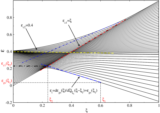
Figure 1: (Color online) Illustration of the tangent method discussed in the text for $\alpha=-0.6$. Energy spectrum of the system in the plane $\varepsilon\times\xi$ where the two ESQPT critical lines are highlighted with red and yellow dashed lines. The dashed blue line is the tangent for the ground state curve $\varepsilon_{gs}(\xi)$ at the point $\xi_{1}$. This shows schematically the graphical determination of the critical quench $\xi_{1}\rightarrow\xi_{2}$ for a given initial state. In general, the intersection of the tangent line with the critical lines provides the critical $\xi_{2}$ value for which the system reaches the ESQPT critical energy after the quench. The dashed blue line stands for the tangent for the highest excited-state curve.

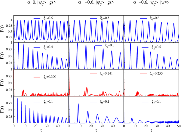
Figure 2: Survival probability $F(t)$ as a function of time ($t$) for a system size $N=300$. The leftmost column includes $F(t)$ results for $\alpha=0$ and the middle and rightmost columns for $\alpha=-0.6$. The initial state for the leftmost and middle columns is the $\xi_{1}=0.6$ Hamiltonian ground state, $|\Psi_{0}\rangle=|gs\rangle$, and the initial state for the rightmost column is the $\xi_{1}=0.7$ Hamiltonian highest excited state, $|\Psi_{0}\rangle=|\Psi^{*}\rangle$, in order to reach the second critical line of the energy spectrum. Different quantum quenches are shown for different values of $\xi_{2}$. There are some critical values for $\xi_{2}$, $\xi_{c}$, for which the system is settled in the critical energy of an ESQPT (third row) and the survival probability drops down to zero (with small random fluctuations).

The Hamiltonian in Eq. (2) depends on two control parameters, $\xi$ and $\alpha$. In general, for negative $\alpha$ values, there exist two different ESQPTs and each one of them has a critical energy line marked by a high level density [33, 38]. Since we are interested in characterizing both ESQPTs, a fixed value of $\alpha<0$ is selected and the time evolution of the system is explored after an abrupt change in the control parameter $\xi$. The aim is to study how the system dynamics is modified by the existence of two critical lines. In the followed quantum quench protocol, the system is initially prepared in a certain normalized eigenstate $|\Psi_{0}\rangle$ of $\hat{H}_{1}=\hat{H}(\xi_{1})$. At time $t=0$ a quantum quench takes place, changing $\xi$ from $\xi_{1}$ to $\xi_{2}$. Thus, the Hamiltonian for the system is now given by $\hat{H}_{2}=\hat{H}(\xi_{2})$ and the initial state, $|\Psi_{0}\rangle$, is no longer an eigenstate of $\hat{H}_{2}$ and, consequently, evolves with time in a non trivial way. The probability amplitude of finding the evolved state, $|\Psi_{0}(t)\rangle$, in the initial state, $|\Psi_{0}\rangle$, can be evaluated easily. The expression for this probability amplitude, denoted as $a(t)$, is $a(t)=\langle\Psi_{0}|\Psi_{0}(t)\rangle$. The survival probability, $F(t)$, also called nondecay probability or fidelity, is given by the absolute square of $a(t)$,

$$F(t)=|a(t)|^{2}=\left|\langle\Psi_{0}|\Psi_{0}(t)\rangle\right|^{2}=\left|\left\langle\Psi_{0}|e^{-\imath\hat{H}_{2}t}|\Psi_{0}\right\rangle\right|^{2}~{}.$$ (4)

Since our goal is to evince the effect on the system dynamics of the external quench when reaching one of the ESQPTs’ critical lines, the determination of suitable $\xi_{2}$ values is very important, since the quenched system has to reach the corresponding critical energies. This can be achieved using the method of the tangent, developed in Ref. [40]. In Fig. 1, a typical evolution of the energy levels, $\varepsilon$, of the Hamiltonian in Eq. (2) is plotted as a function of the control parameter $\xi$, for a value of $\alpha=-0.6$. In this figure, there is a change in the ground state at around $\xi=0.2$ that corresponds to the ground state QPT. In addition, two lines of high level density in the excitation spectra are immediately apparent (separatrices, see Ref. [33]). These lines mark the critical energy of the ESQPTs and separate the phases in such transitions. In the case shown in this figure, the separatrices occur at the critical energies $\varepsilon_{c1}=\xi$ (yellow dashed line) and $\varepsilon_{c2}=0.4$ (red dashed line). A detailed discussion on this structure, including their dependence of the control parameters in the mean field limit, can be found in Ref. [33], where the static properties of the ALMG model are presented. From Fig. 1, it is clear that for analyzing the three phases one has to start from the deformed phase $\xi>\xi_{c}=0.2$. Due to the structure of our Hamiltonian, changing $\xi$ from an initial value $\xi_{1}$ implies that the system is excited along a straight line tangent to the energy line at $\xi_{1}$. Thus, if the initial state is the ground state $|\Psi_{0}\rangle=|gs\rangle$ for a particular $\xi_{1}$ value ($\xi_{1}>0.2$), one needs to find the value of the $\xi$ parameter, $\xi_{2}$, for which the tangent of the initial energy level $\varepsilon_{1}(\xi)$ at $\xi_{1}$ crosses the critical line $\varepsilon_{c}(\xi)$ at $\xi_{2}$ in the plane $\varepsilon\times\xi$. This is illustrated in Fig. 1 for the case in which the eigenstate $|\Psi_{0}\rangle=|gs\rangle$ is the ground state of $H_{1}=H(\xi_{1})$. It is worth noticing that, within the range of values defined for $\xi$, using this method it is not possible to cross both ESQPTs lines from a given initial state. Indeed, for those values of $\xi$ above the value of the critical $\xi_{c}$ for the QPT, it is only possible to reach the first ESQPT, $\varepsilon_{c1}=\xi$, (it can be seen plotting the tangent to the ground state line). It is worth mentioning that if one uses the same tangent method starting from the symmetric phase ($\xi<\xi_{c}=0.2$), one can reach the second ESQPT critical line, $\varepsilon_{c2}=0.4$, (yellow line), but it would be impossible to explore properly its impact on the dynamics of the system since one is forced to move over the first ESQPT critical line (red dashed line). Consequently, the tangent method from the system ground state is suitable for the study of the first ESQPT (red dashed line), but not the second one (yellow dashed line).

Let us first examine the $\varepsilon_{c1}=\xi$ critical line (red dashed line), that can be reached using the tangent method from the $\xi_{1}$ ground state. On the one hand, the energy of the corresponding initial ground state is $\varepsilon_{gs}(\xi_{1})$ and the equation for the tangent line at $\xi_{1}$ for the curve described by the ground state of the system in the $\varepsilon\times\xi$ plane reads $\varepsilon_{t}=m(\xi-\xi_{1})+\varepsilon_{gs}(\xi_{1})$, where $m$ is the slope of the tangent to the ground state curve at $\xi_{1}$. On the other hand, the line of the first ESQPT (red dashed line) is $\varepsilon_{c1}=\xi$. Therefore, both lines cross at

$$\xi_{2}=\xi_{c1}=\frac{m~{}\xi_{1}-\varepsilon_{gs}(\xi_{1})}{m-1},$$ (5)

where $\varepsilon_{gs}(\xi_{1})=\langle gs|\hat{H}_{1}|gs\rangle/N$ (ground state energy per particle at $\xi_{1}$) and the slope $m$ of the tangent line is obtained making use of the Hellman-Feynman theorem in Eq. (2). Indeed, $m=\left\langle gs|\hat{H}^{\prime}|gs\right\rangle/N=d\varepsilon_{gs}(\xi)/d\xi|_{\xi=\xi_{1}}$, where $\hat{H}^{\prime}=\frac{2}{S}\left(S^{2}-\hat{\mathcal{S}}_{x}^{2}\right)^{2}-(S+\hat{\mathcal{S}}_{z})$.

A similar analysis can be performed for the anharmonicity-induced critical line. However, as we noticed above, the tangent to any point along the ground state line with $\xi>\xi_{c}$ never crosses the second critical line (dashed yellow line) for the range of values of $\xi$ considered in this model. Hence, to explore this separatrix one should start from a more appropriate $\hat{H}_{1}$ eigenstate. In particular, we have selected the highest excited state (denoted as $|\Psi^{*}\rangle$). As with the ground state, the most excited state of our system is well-defined in the thermodynamic limit by a coherent-state [42]. Then, our initial state is now $|\Psi_{0}\rangle=|\Psi^{*}\rangle$ of $\hat{H}_{1}$. Let us denote the slope of the tangent to the energy line of the highest state at $\xi_{1}$ as $m_{2}$. Then, this tangent line will reach the anharmonicity-induced ESQPT line given by $\varepsilon_{c2}=\varepsilon_{0}$ which is a constant. In the $\alpha=-0.6$, the value of $\varepsilon_{0}=0.4$ was computed with a mean field formalism [33]. Therefore, the value for the critical $\xi$, $\xi_{c2}$, reads

$$\xi_{c2}=\frac{m_{2}~{}\xi_{1}+\varepsilon_{0}-\varepsilon_{\Psi^{*}}(\xi_{1})}{m_{2}},$$ (6)

where $\varepsilon_{\Psi^{*}}(\xi_{1})=\langle\Psi^{*}|\hat{H}_{1}|\Psi^{*}\rangle/N$ and $m_{2}=\left\langle\Psi^{*}|\hat{H}^{\prime}|\Psi^{*}\right\rangle/N=d\varepsilon_{\Psi^{*}}(\xi)/d\xi|_{\xi=\xi_{1}}$ is the slope of the corresponding tangent line.

Once a way of crossing both ESQPT lines is available, the dynamic evolution of the system and the effect of crossing an ESQPT line can be examined. This can be accomplished computing the survival probability $F(t)$ Eq. (4). Results for $F(t)$ as a function of time are shown in Fig. 2 for $N=300$, $\alpha=0$ (left column) and $-0.6$ (center and right columns) and different initial states (either the ground state $|\Psi_{0}\rangle=|gs\rangle$ in the left and central columns or the most excited state $|\Psi_{0}\rangle=|\Psi^{*}\rangle$ in the right column) for selected $\xi-$values. The $\alpha=0$ case in the leftmost panels is included for the sake of completeness and reference. The panels in this column depict the time evolution of the survival probability for decreasing values of $\xi_{2}$, starting always from the ground state $\ket{gs}$ for $\xi_{1}=0.6$. The calculated $\xi_{2}$ at the crossing with the ESQPT is $\xi_{c}=0.3$. In general, the survival probability has a regular oscillatory behaviour except in the region close to the ESQPT critical energy, $\xi_{2}=0.3$, where the system undergoes an ESQPT and the survival probability suddenly drops down to zero and starts to oscillate randomly with small amplitudes. Once the critical energy for the ESQPT is crossed, the survival probability starts to oscillate in a regular way again. This phenomenon was reported for the first time in Ref. [28]. In the central and rightmost columns the same observable is plotted including a non-zero anharmonic term ($\alpha=-0.6$).

In the panels of the second column of Fig. 2, the survival probability is depicted for decreasing values of $\xi_{2}$ and starting always from the ground state of a Hamiltonian with $\xi_{1}=0.6$ and $\alpha=-0.6$. Due to the negative $\alpha$ value, the system undergoes two ESQPTs, displayed in the spectrum by means of critical lines with a noteworthy accumulation of energy levels (see Fig. 1). One of the two critical lines (red dashed line) can be traced back to the ESQPT already present in the $\alpha=0$ case [25]. However, the second one (yellow dashed line) is linked to the presence of the anharmonic term in the Hamiltonian [33]. The nature and physical interpretation of the anharmonicity-induced ESQPT is different from the already known ESQPT associated with the ground state QPT. Hence, in principle, there is no a-priori reason for both behaving in the same way. However, as we see if we compare the results for the critical $\xi_{c}$ values in the different columns, the results obtained for the $\alpha=0$ and the anharmonic cases are similar. The survival probability is oscillatory and regular except once $\xi_{2}$ is close to $\xi_{c}$, the critical value for the first or second ESQPT. In all cases, when $\xi_{2}=\xi_{c}$, the quenched system reaches the critical energy and the survival probability suddenly drops down to zero and oscillates randomly with a small amplitude (red curves). This is similar to what happens in the $\alpha=0$ case. Once $\xi_{2}$ is smaller than $\xi_{c}$, a periodic oscillatory decaying behaviour is observed in $F(t)$. As explained above, the quench from the ground state never reaches the second ESQPT line. For that purpose, one has to start from a different initial state. Thus, in order to explore how $F(t)$ is affected by the second ESQPT, the quantum quench is performed using as an initial state the highest excited state of the system, $|\Psi^{*}\rangle$, for a given value of $\xi_{1}$. In this way, the second critical line (yellow dashed line) for the ESQPT is accessible after the quench. In the panels of the right column of Fig. 2, the survival probability for decreasing $\xi_{2}$ values is plotted for an initial state equal to the highest excited state of the Hamiltonian with $\xi_{1}=0.7$ and $\alpha=-0.6$. For this parameter selection, the second critical line is reached at $\xi_{c}=0.255$. In this column, again, results are very similar to the ones obtained in the preceding cases. The fidelity $F(t)$ oscillates regularly while $\xi_{2}>\xi_{c2}$, but when the $\xi_{2}$ parameter gets close to the critical value, $\xi_{c2}=0.255$, the survival probability drops down to zero and randomly oscillates with a small amplitude. Once the critical line is crossed, $F(t)$ recovers an oscillatory decaying periodic behavior, but at a certain time, this periodic oscillatory behaviour becomes distorted. The reason for this phenomenon is that the tangent line to the highest excited state curve at $\xi_{1}$ in the plane $\varepsilon\times\xi$ remains very close to the critical line $\varepsilon_{c2}=0.4$ after the quench for lower values of $\xi_{2}$ up to 0. One should note that when starting from the highest excited state the first ESQPT critical line is not accessible after the quench (see Fig. 1).

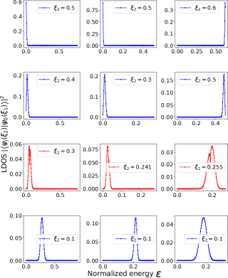
Figure 3: LDOS $\left|\innerproduct{\psi_{j}(\xi_{2})}{\psi_{0}}\right|^{2}$ as a function of the normalized excitation energy $\varepsilon_{j}$ (arb. units) for systems with $\xi_{1}=0.6$ and $\alpha=0.0$ (left column), $\xi_{1}=0.6$ and $\alpha=-0.6$ (middle column), and $\xi_{1}=0.7$ and $\alpha=-0.6$ (right column) ($N=300$ in all cases). The chosen states are the ground state $\ket{\psi_{0}}=\ket{\text{gs}(\xi_{1})}$ (left and middle columns) and the most excited state with even parity $\ket{\psi_{0}}=\ket{\Psi^{*}(\xi_{1})}$ (right column), expressed in all cases in the basis of eigenstates of the Hamiltonian $\hat{H}(\xi_{2},\alpha)$, being $\xi_{2}$ the quench parameter. The cases that correspond to a critical value of $\xi_{2}$ (third row) are plotted using red color.

If we denote the eigenstates of $\hat{H}(\xi_{i},\alpha)$ with $i=1,2$ as $\ket{\psi_{j}(\xi_{i})}$ with $j=0,1,\ldots,N/2$, then we can write the initial state $\ket{\Psi_{0}}$ in the basis of $\hat{H}_{2}=\hat{H}(\xi_{2},\alpha)$ eigenfunctions as $\ket{\Psi_{0}}=\sum_{j}C_{j}\ket{\psi_{j}(\xi_{2})}$ and then

$$F(t) =\left|\left\langle\Psi_{0}|e^{-\imath\hat{H}_{2}t}|\Psi_{0}\right\rangle\right|^{2}$$

$$=\left|\sum_{j}\left|C_{j}\right|^{2}e^{-iE_{j}t}\right|^{2}=\left|\int dEe^{-iEt}\rho_{0}(E)\right|^{2}~{},$$ (7)

where $E_{j}$ is the energy of the $j$-th $\hat{H}_{2}$ eigenstate and $\rho_{0}(E)=\sum_{j}\left|C_{j}\right|^{2}\delta(E-E_{j})$, called the strength function or local density of states (LDOS) [43, 44], is the energy distribution of $\ket{\Psi_{0}}$ weighted by the $C_{j}$ components.

From Eq. (7) it is clear that the fidelity $F(t)$ is the absolute value of the LDOS Fourier transform squared and this quantity can provide some clues on the $F(t)$ time dependence for the quench at the critical values $\xi_{c}$, denoted in red in the third row of Fig. 2. In Fig. 3 we plot the LDOS for the same cases included in Fig. 2, hence in the first column, we show the LDOS for the ground state of $\hat{H}_{1}=\hat{H}(\xi_{1}=0.6,\alpha=0)$ for different $\hat{H}_{2}$ cases, all of them with $\alpha=0$. In the second and third columns we depict the LDOS for initial states that are the ground state of $\hat{H}_{1}=\hat{H}(\xi_{1}=0.6,\alpha=-0.6)$ and the most excited state of $\hat{H}_{1}=\hat{H}(\xi_{1}=0.7,\alpha=-0.6)$. The LDOS for the critical quench values are depicted in red. It can be clearly seen that, for all columns, in the critical control parameter cases the LDOS is nonzero at the ESQPT critical energy and has a clear local minimum at this energy value. The Fourier transform of such LDOS produces the particular time dependence shown in the panels of the Fig. 2 third row.

Another quantity of interest, inspired on Loschmidt’s objections to Boltzmann H theorem, is the Loschmidt echo [45, 46]. This quantity, considered a probe to the sensibility of a system dynamics under perturbations, is used to benchmark the reliability of quantum processes [47]. It was shown to be a valid QPT detector [48] and, more recently, it has been used to check the influence of the ESQPT on the dynamics of the LMG model [49]. Consider an initial wave function, $\ket{\psi}$, which evolves a time $t$ under a Hamiltonian $\hat{H}_{1}$, $\ket{\psi(t)}=e^{-i\hat{H}_{1}t}\ket{\psi}$. We can reverse the time evolution with another Hamiltonian $\hat{H}_{2}$, $e^{i\hat{H}_{2}t}e^{-i\hat{H}_{1}t}\ket{\psi}$. The squared overlap of the resultant state with the initial state $\ket{\psi}$ is the Loschmidt echo (LE), denoted as $M(t)$ [46, 50],

$$M(t)=\left|\bra{\psi}e^{i\hat{H}_{2}t}e^{-i\hat{H}_{1}t}\ket{\psi}\right|^{2}~{}.$$ (8)

Another physical interpretation of this quantity is possible, since Eq. (8) is the distance between the same initial state once it is evolved for a time $t$ with two different Hamiltonian operators. One of the properties of ground state and excited state QPTs is that, near the critical region, states are quite sensitive to perturbations. A way to quantify this effect is computing the LE for the eigenstates of the system $\hat{H}_{1}=\hat{H}(\xi,\alpha)$ with a time-reversal under $\hat{H}_{2}=\hat{H}(\xi+\delta,\alpha)$,

$$M_{j}(t)=\left|\left\langle\psi_{j}(\xi,\alpha)\left|e^{i\hat{H}(\xi+\delta,\alpha)t}\right|\psi_{j}(\xi,\alpha)\right\rangle\right|^{2}~{},$$ (9)

where $\ket{\psi_{j}(\xi,\alpha)}$ is the $j$-th eigenstate of $\hat{H}_{1}$ and $\delta$ is a small perturbation. The LE, as well as its long-time average value, detects the ESQPT in the LMG model without anharmonicity [49].

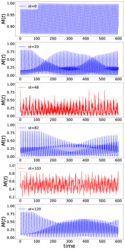
Figure 4: Loschmidt echoes for a system with $\xi=0.3$, $\alpha=-0.6$, $N=300$, and a perturbation across the control parameter $\xi$ of $\delta=0.01$. From top to bottom we display $M_{j}(t)$ for the $j$-th state with even parity: $0$, $20$, $48$, $82$, $103$ and $120$. The states closer to the ESQPTs are plotted in red.

In Fig. 4 we plot $M_{j}(t)$ for several eigenstates of a system with $\xi=0.3$ and $\alpha=-0.6$. The total number of bosons is $N=300$, the system has been perturbed with $\delta=0.01$, and only states with even parity are considered. Results are shown for $j=0,~{}20,~{}48,~{}82,~{}103$, and $120$. The two states with energies closest to ESQPTs critical energies ($j=48$ and $103$) are plotted in red. As expected, the ground state $j=0$ perform small oscillations with a single frequency around a value close to one, with a maximum value equal to one. Other states far from the critical region, as $j=20,~{}82$, and $120$, have a more complex oscillation pattern, not harmonic, with a larger amplitude and without reaching unity in the considered time range. However, in the case of eigenstates close to the critical energy, $j=48$ and $103$, $M(t)$ is only one for $t=0$ and the oscillations of the LE are of a much more irregular nature, something similar to what happens for the fidelity $F(t)$ in Fig. 2.

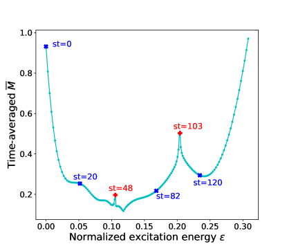
Figure 5: Time-averaged of $M(t)$ versus the normalized excitation energy $\varepsilon$ for the same system introduced in Fig. 4. The highlighted states (red plus symbols for transition states and blue crosses for others) correspond to the states studied in Fig. 4.

As shown in Ref. [49], the time averaged value of the LE for the $j$-th eienstate, $\overline{M}_{j}$, is a convenient probe to detect an ESQPT. This quantity is defined as

$$\overline{M}_{j}=\lim_{T\to\infty}\frac{1}{T}\int_{0}^{T}dt~{}M(t)=\sum_{k}\absolutevalue{c_{jk}^{\delta}}^{4}~{},$$ (10)

where $c_{jk}^{\delta}$ are the coefficients of the $j$-th eigenfunction of the Hamiltonian operator $\hat{H}(\xi+\delta,\alpha)$, expressed in the basis of eigenstates of $\hat{H}(\xi,\alpha)$: $\ket{\psi_{j}(\xi+\delta,\alpha)}=\sum_{k}c_{jk}^{\delta}\ket{\psi_{k}(\xi,\alpha)}$. The LE time averaged value is equal to the inverse of the participation ratio (PR) of $\ket{\psi_{j}(\xi+\delta,\alpha)}$ computed using the basis $\left\{\ket{\psi_{k}(\xi,\alpha)}\right\}$. In Fig. 5 we plot the time averaged LE versus the normalized excitation energy for all even parity states of the system studied in Fig. 4. The states included in Fig. 4 have been marked using red pluses for critical ones ($j=48$ and $103$) and blue crosses for others ($j=20,~{}82$, and $120$). $\overline{M}_{j}$ has local maxima located for the eigenstates close to the critical energies, as it was observed in the LMG model without anharmonicity [49]. Hence, the time averaged LE detects the new ESQPT associated to the anharmonic term in the LMG Hamiltonian and confirms that this quantity is a good ESQPT probe.

IV ESQPTs and OTOC

Out-of-time-order correlators (OTOCs), that appeared for the first time in the ’60s in the context of superconductivity [52], are a four-point temporal correlation function able to measure the entanglement spread in a quantum system from the degree of noncommutativity in time between operators. Since then, after a long period of relative inactivity, there has been a tremendous frenzy around this concept on various fronts [53]. They returned to the limelight with the proposal of OTOCs as a viable quantum chaos indicator, due to its exponential increase at early times in certain systems [54, 55, 56, 57], and to diagnose the scrambling of quantum information [58, 59, 60, 61]. Besides, OTOCs are sensitive probes for quantum phase transitions [62, 63, 64, 65, 66, 67, 68]. Despite the fact that the experimental access to out-of-time-order correlators is hindered by the unusual time ordering of its constituents operators that precludes the measurement using local operators, several approaches using different experimental platforms have successfully provided OTOC results [69, 70, 71, 72, 73, 74, 75, 23].

Given two operators, $\hat{W}$ and $\hat{V}$, it is possible to probe the spread of $\hat{W}(t)$ with $\hat{V}$ through the expectation value of the square commutator

$${\cal C}_{w,v}(t)=\left\langle\left[\hat{W}(t),\hat{V}(0)\right]^{\dagger}\left[\hat{W}(t),\hat{V}(0)\right]\right\rangle,$$ (11)

where $\hat{W}(t)=e^{\imath\hat{H}t}\hat{W}e^{-\imath\hat{H}t}$ is the operator $\hat{W}$ in the Heisenberg’s representation [53, 76, 77, 78, 79]. The expectation value is usually computed in the canonical ensemble. However, in recent works, it has also been computed over given initial states or over the system eigenstates (microcanonical OTOC) [77, 78]. The squared commutator Eq. (11) can be rewritten as ${\cal C}_{w,v}(t)={\cal A}_{w,v}(t)-2{\cal F}_{w,v}(t)$. The first term is a two-point correlator, ${\cal A}_{w,v}(t)=\left\langle\hat{W}^{\dagger}(t)\hat{V}^{\dagger}(0)\hat{V}(0)\hat{W}(t)\right\rangle+\left\langle\hat{V}^{\dagger}(0)\hat{W}^{\dagger}(t)\hat{W}(t)\hat{V}(0)\right\rangle$ and the out-of-time order appears in ${\cal F}_{w,v}(t)$, the real part of a four-point correlator

$${\cal F}_{w,v}(t)=\real\left[\left\langle\hat{W}^{\dagger}(t)\hat{V}^{\dagger}(0)\hat{W}(t)\hat{V}(0)\right\rangle\right].$$ (12)

Without loss of generality, if we consider operators that are unitary, then Eq. (11) reads ${\cal C}_{w,v}(t)=2-2{\cal F}_{w,v}(t)$.

In a recent LMG model study, the ESQPT effects on the microcanonical OTOC and the OTOC following a quantum quench were explored for $\hat{W}=\hat{V}=\hat{\mathcal{S}}_{x}/S$ [64]. The time evolution of the OTOC after a sudden quench was analyzed and it was concluded that the equilibrium value (the long time average value) of this observable can be used as a good marker for the ESQPT because it behaves as an order parameter, able to distinguish between the phases below and above the ESQPT, respectively. Our goal, here, is to analyze how the OTOC behaves once the ALMG system goes through the anharmonicity-induced ESQPT line. This study is of relevance since the physical nature of this ESQPT is different from the one of the already known ESQPT for the usual LMG model. Moreover, the possibility of using an OTOC as an order parameter for both ESQPTs is considered.

We have used in our analysis the microcanonical OTOC [77, 80], defined as

$${\cal F}_{n}(t)=\real\left[\langle n|\hat{W}^{\dagger}(t)\hat{V}^{\dagger}(0)\hat{W}(t)\hat{V}(0)|n\rangle\right]~{},$$ (13)

where the state $\ket{n}$ is the $n$-th eigenstate of the Hamiltonian Eq. (2), whose energy is $E_{n}$. This state is computed for a given set of Hamiltonian parameters, $\xi$ and $\alpha$.

Following Ref. [64], we have first selected $\hat{W}=\hat{V}=\hat{\mathcal{S}}_{x}/S$ as the OTOC operators. The reason behind this election is twofold. On the first hand, the expectation value of the $\hat{\mathcal{S}}_{x}$ operator is known to be an order parameter for the QPT in the LMG model, and it has also been shown in previous works that it behaves as an order parameter for the ESQPT [81]. On the second hand, the $\hat{\mathcal{S}}_{x}$ operator is related with the breaking of parity symmetry in the spectrum eigenstates [43]. However, the obtained results (not shown) indicate that in this case the $F_{n}(t)$ equilibrium value only detects the occurrence of the first ESQPT, independently of its nature, and not the second one. We decided to explore other possibilities such as $\hat{W}=\hat{\mathcal{S}}_{y}/S$, $\hat{V}=\hat{\mathcal{S}}_{x}/S$ or $\hat{W}=\hat{\mathcal{S}}_{+}/S$, $\hat{V}=\hat{\mathcal{S}}_{-}/S$. In both cases we obtain the expected results, with equilibrium values sensitive to the anharmonicity-induced ESQPT in the symmetric phase and to the two ESQPTs in the broken symmetry phase.

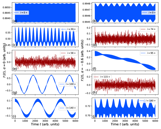
Figure 6: (Color online) Time evolution of the microcanonical OTOC, ${\cal F}_{i}(t)$, for selected positive parity eigenstates of an ALMG model with a system size $N=300$. In all panels $\xi=0.5$, the left column panels refers to ${\cal F}_{i}(t)$ for $\alpha=0$ and the right column panels include results for $\alpha=-0.6$. OTOCs for different initial states are shown: for the left column from top to bottom; (a) $\ket{i=0}$ (ground state), (c) $\ket{i=30}$, (e) $\ket{i=58}$, (g) $\ket{i=100}$, and (e) $\ket{i=140}$. For the right column from top to bottom: (b) $\ket{i=0}$ (ground state), (d) $\ket{i=74}$, (f) $\ket{i=95}$, (h) $\ket{i=115}$, (j) $\ket{i=140}$. There are some energies in which the eigenstate is settled at the critical energy of an ESQPT. These are the cases for panels (e) in the left column and (d) and (h) in the right column, highlighted using a red color.

Numerical solutions for the time evolution of the OTOC Eq. (13) with $\hat{V}=\hat{\mathcal{S}}_{-}/S$ and $\hat{W}=\hat{\mathcal{S}}_{+}/S$ are presented in Fig. 6. These are results for a selected set of positive parity states of a system with size $N=300$ that are obtained by the diagonalization of the Hamiltonian Eq. (2). The time evolution of the microcanonical OTOC is depicted for different initial states and $\xi=0.5$ with either $\alpha=0$ (left-column panels) or $\alpha=-0.6$ (right-column panels). Despite the different operators included in the OTOC, a quite similar phenomenology to that pointed out in Ref. [64] is observed. However, it is worth to emphasize that if we kept $\hat{V}=\hat{W}=\hat{\mathcal{S}}_{x}/S$, once the first critical energy is crossed, the time average value of the OTOC is zero as ${\cal F}_{n}(t)$ oscillates around zero.

The behaviour of the microcanonical OTOC, ${\cal F}_{i}(t)$, depends on the region of the spectrum in which the system is located. Particularly, ${\cal F}_{i}(t)$ develops a regular behavior, with small amplitude oscillations around a positive value. This value decreases until the ${\cal F}_{i}(t)$ oscillates around zero, when the critical energy value is reached. For the states close to the ESQPT critical energy (red color curves), not only ${\cal F}_{i}(t)$ oscillates around zero, but it also behaves in a highly irregular way, as in Ref. [64]. This is a feature shared by both columns in Fig. 6, though in the right column panels the second and fourth panel correspond to critical energies for the two ESQPTs that arise in this case.

Let us now to discuss in more detail the left column ($\alpha=0$). Remind that in this case there is just one ESQPT located in the mean field limit at energy $\varepsilon=\xi$, its value for these plots is $\varepsilon=\xi=0.5$. We have selected the ground state and four other positive parity eigenstates, $i=0$, $30$, $58$, $100$, and $140$ in panels (a), (c), (e), (g), and (i), respectively. The state with the closer energy to the critical ESQPT energy is $i=58$ –panel (e)– where the ESQPT precursors are clearly manifested. In the cases with energies below the critical energy ${\cal F}_{i}(t)>0$. However, as can be seen in panel (e), once the critical energy for the ESQPT is reached, the OTOC oscillates randomly around zero. For energies larger than the critical energy –left panels (g) and (i)– the ${\cal F}_{n}(t)$ display high and low frequency oscillations around a zero mean value. Therefore, the steady-state value of ${\cal F}_{n}(t)$ will be equal to zero for these states. As one goes up in energy in the spectrum, the same kind of oscillatory behavior is observed, with smaller amplitudes.

There are some new features arising in the right column panels, that include ${\cal F}_{i}(t)$ results for the $\alpha=-0.6$ anharmonic case. As previously mentioned, in this case there are two critical ESQPT lines that in the mean field limit lie at $\varepsilon=1+\alpha=0.4$ and $\varepsilon=\xi=0.5$. We show the results for the two eigenstates with local minimum PR values $i=74$ and $115$ in panels (d) and (h) of the right column in Fig. 6. Again, the ${\cal F}_{i}(t)$ OTOC oscillations at the critical lines are markedly irregular. These two states have been highlighted using red color. The other three values included in the right column of Fig. 6 are $i=0$ (ground state), $95$, and $140$. In the region between the two critical lines, the envelope for ${\cal F}_{i}(t)$ has a sine-like oscillatory behaviour around zero, so its steady-state value equals zero. Once the second critical line is crossed and the system energy increases, ${\cal F}_{i}(t)$ presents again an oscillatory behaviour around positive values, as can be clearly seen in Fig. 6. It is worth pointing out that the characteristic times of the different microcanonical OTOCs span a wide range of frequencies. In particular, panel (f) in Fig. 6 exhibits a much longer period (smaller frequency) than the rest of the panels. The oscillatory frequency of the four-point correlator can be traced back to energy differences between pairs of states of different parity [68]. Therefore, whenever different parity eigenstates are degenerate, the stationary value of the OTOC has a non-zero contribution. This occurs at energies less than the critical energy of the first ESQPT and above the critical energy of the second ESQPT. The OTOC associated with eigenstates whose energies are either just under the critical energy of the first ESQPT or above the critical energy of the second ESQPT have small frequencies due to the small energy differences because the degeneracy starts splitting. A similar small-frequency OTOC can be observed for energies in between both ESQPTs —as shown in Fig. 6 panel (f)—. In this case, positive- and negative-parity states are non-degenerate. However, there are states whose energy gaps with the adjacent states of opposite parity are very close. In such cases, some OTOC frequencies can again be very small, and thus the correlator may exhibit a long-period oscillation around zero, depending on the value of the matrix elements of the operators $\hat{V}$ and $\hat{W}$.

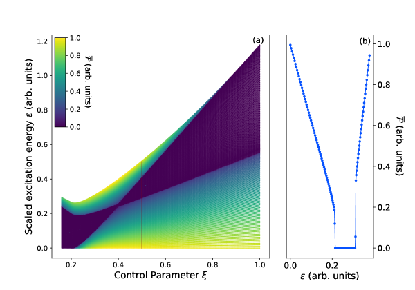
Figure 7: Panel a: Correlation energy diagram of the even parity states ALMG model as a function of the the control parameter $\xi$ with $\alpha=-0.6$. Each energy level is colored according to the steady-state value of the microcanonical OTOC, $\overline{{\cal F}}_{j}$, where $j$ takes the values $i=0,1,\ldots,N/2$. A vertical line marks the results for the $\xi=0.5$ case whose $\overline{{\cal F}}_{j}$ are depicted in the right panel. Panel b: Steady-state value of the microcanonical OTOC, $\overline{{\cal F}_{j}}$, as a function of the re-scaled excitation energy $\overline{\varepsilon}$ for even parity states of a system with control parameters $\xi=0.5$ and $\alpha=-0.6$. Both panels: Calculations for a system with size $N=400$.

It is worth noticing that, in the anharmonic case, the two ESQPT critical lines cross at $\xi=0.4$, as we can observe in Fig. 1. Since the case depicted in Fig. 6 is for $\xi=0.5$, going up in energy from the ground state the first ESQPT found is the anharmonic one (not present in the simple LMG model). We have checked, although it is not shown here, that similar results are obtained if we consider a value of $\xi$ such that the two critical lines have not crossed yet ($\xi-$value between $0.2$ and $0.4$). This is interesting because, regardless the physical origin of the critical line, once the first ESQPT critical line is crossed, the microcanonical OTOC starts oscillating around zero until the second ESQPT critical energy is crossed. This has an immediate consequence on the steady-state value of ${\cal F}_{i}(t)$ for $\hat{V}=\hat{\mathcal{S}}_{-}/S$ and $\hat{W}=\hat{\mathcal{S}}_{+}/S$, that can be taken as a reliable order parameter. This is not the case for $\hat{W}=\hat{V}=\hat{\mathcal{S}}_{x}/S$. It is true that this choice of operators marks correctly the transition once the first critical line is crossed, but it is not sensitive to the second ESQPT critical line, irrespective of the physical origin.

The steady state of the microcanonical OTOC ${\cal F}_{i}(t)$ is defined as

$$\overline{{\cal F}}_{i} = \lim_{T\to\infty}\frac{1}{T}\int_{0}^{T}{\cal F}_{i}(t)dt~{}.$$ (14)

Results for this quantity can be found in Fig. 7. In the left panel we depicted the correlation energy diagram for a system with size $N=400$ as a function of the $\xi$ parameter for a fixed anharmonicity parameter value $\alpha=-0.6$. Each point is colored according to the corresponding $\overline{{\cal F}}_{i}$ value. From this figure it is clear how the stationary limit of the OTOC provides a convenient order parameter for the two ESQPTs in the ALMG model, with abrupt changes whenever the system gets through critical energies. The right panel of the same figure (Fig. 7b) includes the stationary OTOC results for the eigenstates of an ALMG model with system size $N=400$ and control parameters $\xi=0.5$ and $\alpha=-0.6$ as a function of the re-scaled energy the rescaled excitation energy $\varepsilon_{n}=(E_{n}-E_{gs})/N$. This corresponds to the results marked with a vertical line in Fig. 7a. The energy dependence of this quantity can be anticipated from the observation of the behavior of ${\cal F}_{i}(t)$ depicted in Fig. 6. Indeed, as pointed out previously, the main feature of ${\cal F}_{i}(t)$ is that it is an oscillatory function. However, the value around which it oscillates is different from zero only in the region below (above) the critical energy of the first (second) ESQPT that is encountered when one goes up in energy in the spectrum. Once the first ESQPT critical line is crossed, regardless of its physical origin, the oscillations are around zero. This leads to the conclusion that $\overline{{\cal F}}_{i}$ is different from zero in the region below the first critical line and it is equal to zero in the region of the spectrum above that first ESQPT critical line. However, it is worth noticing that for particular values of the control parameters there could be nonzero instances of $\overline{{\cal F}}_{i}$. These nonzero values are isolated, akin to accidental degeneracies and are not associated to a critical energy, thus are easily distinguishable from the sudden change associated with the occurrence of an ESQPT.

In light of these results, it is clear that ESQPTs have a strong impact on the OTOC dynamics, notwithstanding they can be mapped to a stationary point or the asymptotic behavior of the PES in the semiclassical description of the system. Thus, the findings given in Ref. [64] are confirmed in this respect. However, concerning the use of $\overline{{\cal F}}_{i}$ as an order parameter, we have found that to be sensitive to both ESQPT lines the $\hat{W}$ and $\hat{V}$ operators cannot be the same.

V Conclusions

The ALMG model presents, in addition to the ground state QPT and its known ESQPT, a second ESQPT. In this work, we have analyzed the impact of both ESQPT critical lines on the dynamical evolution of the survival probability, the Loschmidt echo and the OTOC. We have found that both ESQPTs, despite of having different physical origins, lead to a dramatic change in the survival probability evolution after a quantum quench. Particularly, it has been shown that the survival probability gives information about system relaxation: for a certain critical quench, related to the ESQPT energy, the system behaves in a unique way that allows one to recognize the critical lines separating regions in which the system is in a different phase. In addition, it has been explained that due to the way we are introducing the quantum quench it does not allow to reach with the same procedure the two ESQPT lines that appear in the anharmonic Lipkin model. Consequently, an alternative way for characterize one ESQPT has been proposed. This method starts from the most excited Hamiltonian eigenstate (instead of the ground state). Both calculations are complementary and allow us to study the two ESQPT lines. In both cases, the survival probability drops down to zero (with small random fluctuations) when reaching an ESQPT line. This behavior was explained with the help of the LDOS.

We show that other quantity whose evolution is greatly affected by the presence of an ESQPT is the LE (see Figs. 4 and 5). The time-dependence of the LE is quite different if the evolved state is close to the critical energy. Beyond the temporal evolution, the time-averaged LE has been proved to be a convenient ESQPT detector in the ALMG model too, since this quantity displays local maxima in the critical ESQPT energy values.

An additional way of characterizing the dynamical evolution of the system is the study of an OTOC. In this work, such a study has been done using the microcanonical scheme and has revealed that the new ESQPT, that is, the one generated by the anharmonicity term, also has noticeable effects on the evolution of the OTOC. However, it is difficult to determine sharply if the system has reached the critical ESQPT energy, since there is a wide region close to the critical energy where the system is affected by the corresponding ESQPT. Finally, we have concluded that the normalized steady-state value for ${\cal F}_{i}(t)$, $\overline{{\cal F}}_{i}$, can be used as an order parameter to mark the two ESQPTs that occur in the ALMG, despite the different nature of the two cases.