Detecting Grouped Local Average Treatment Effects and Selecting True Instruments
With an Application to Estimating the Effect of Prison on Recidivism

Abstract

Under an endogenous binary treatment with heterogeneous effects and multiple instruments, we propose a two-step procedure for identifying complier groups with identical local average treatment effects (LATE) despite relying on distinct instruments, even if several instruments violate the identifying assumptions. We use the fact that the LATE is homogeneous for instruments which (i) satisfy the LATE assumptions (instrument validity and treatment monotonicity in the instrument) and (ii) generate identical complier groups in terms of treatment propensities given the respective instruments. We propose a two-step procedure, where we first cluster the propensity scores in the first step and find groups of IVs with the same reduced form parameters in the second step. Under the plurality assumption that within each set of instruments with identical treatment propensities, instruments truly satisfying the LATE assumptions are the largest group, our procedure permits identifying these true instruments in a data driven way. We show that our procedure is consistent and provides consistent and asymptotically normal estimators of underlying LATEs. We also provide a simulation study investigating the finite sample properties of our approach and an empirical application investigating the effect of incarceration on recidivism in the US with judge assignments serving as instruments.

1 Introduction

Instrumental variables (IV) analysis is a well-established method to estimate the effect of a treatment on an outcome in presence of unobserved confounding. In a model with a single endogenous treatment and multiple IVs, different instruments can identify heterogeneous local average treatment effects (LATE) given that they satisfy the following LATE assumptions of Imbens and Angrist (1994) and Angrist, Imbens, and Rubin (1996):

1. the instruments are associated with the treatment (relevance)

2. the instruments are as good as random, i.e., not influenced by unobserved characteristics affecting the outcome (exogeneity)

3. the instruments do not have an effect on the outcome other than through the treatment, neither directly, nor through unobservables (exclusion)

4. there exist no defiers, i.e., subjects whose treatment state is reduced when increasing an instrument (monotonicity).

Recent advances in parametric statistics focused on separating valid instruments from invalid ones that violate (b) and (c), but did not consider the case of heterogeneous treatment effects. In this paper, we propose a method for detecting IVs that satisfy the LATE assumptions (b), (c), and (d) in heterogeneous treatment effect models among a set of candidate instruments that may also contain invalid IVs not satisfying the LATE assumptions. Our approach relies on the following two conditions. First, there must exist clusters of IVs which generate identical first stages, i.e., conditional treatment probabilities given the instrument. Second, the LATE assumptions must hold for a plurality (i.e., relative majority) of IVs within such clusters.

Our methodological contribution to the literature on valid IV selection consists of allowing for the presence of heterogeneous first stage effects (of the instruments on the treatment) and of heterogeneous treatment effects on the outcome and proceeds in two steps. In the first step, we make use of Agglomerative Hierarchical Clustering (AHC, Ward, 1963) to find clusters –which we call clubs– of IVs with identical conditional treatment probabilities, henceforth referred to as propensity scores, in order to generate homogeneous complier groups when pairing these clubs. The underlying intuition is that if two distinct IV pairs entail the same higher and lower propensity scores, then the complier groups in either pair must be identical in terms of unobserved characteristics if the LATE assumptions hold. Therefore, our approach permits clustering IVs into club-pairs with homogeneous LATEs if the IV exclusion restriction, exogeneity, and montonicity hold. We stress that the key assumption underlying this step is that propensity scores defining the first-stage effect of the instrument on the treatment are indeed clustered in the population. In the second step, within a specific club, we distinguish valid and invalid IVs, which violate one or multiple LATE assumptions, based on the plurality assumption. The latter states that the largest group of IVs within a club satisfies the LATE assumptions and thus, entails the same LATE, where a group is defined as a set of IVs with identical reduced form estimands, i.e., the expected outcomes conditional on the IVs. We determine the set of valid IVs by hierarchically clustering reduced form estimates within clubs (defined on first stages) and selecting the cluster containing the relative majority of IVs.

Our two-step procedure broadly fits into the fast evolving literature on the integration of machine learning methods in causal inference, by applying unsupervised machine learning for clustering compliers based on the first stage effects of IVs and selecting IVs that satisfy the identifying assumptions, respectively. We show that under certain regularity conditions, the first-step selection procedure consistently classifies propensity scores into clubs (if clubs exist), while the second-step selection procedure consistently detects those IVs which satisfy the LATE assumptions (if plurality holds). Furthermore, we investigate the finite sample behavior of our method in a simulation study and find it to perform well even under a relatively moderate number of observations per instrument in terms of first- and second-step clustering, when a subset of instruments violates the exclusion restriction.

Our study contributes to a growing literature on detecting and selecting valid and invalid IVs (Kang, Zhang, Cai, and Small, 2016; Windmeijer, Farbmacher, Davies, and Smith, 2019; Guo, Kang, Cai, and Small, 2018; Windmeijer, Liang, Hartwig, and Bowden, 2021; Apfel and Liang, 2021) under the assumption that at least a subset of instruments is valid, following the seminal work of Andrews’ (1999). A drawback of previously available IV selection approaches is that they impose homogeneous treatment effects and thus, LATEs and can for this reason not distinguish violations of an identifying assumption from effect heterogeneity. Furthermore, the methods do generally not allow for simultaneous violations of the exclusion restriction and IV exogeneity (Apfel and Windmeijer, 2022). Finally, they do not consider violations of treatment monotonicity in the instrument as discussed in Imbens and Angrist (1994). We are the first to consider violations of both the IV assumptions and the homogeneity of treatment effects. More specifically, our method aims to simultaneously detect groups with distinct LATEs and instruments subject to violations of any of the LATE assumptions (while other contributions focus on a subset of IV assumptions like the exclusion restriction). Sun and Wüthrich (2022) propose a technique exploiting testable conditions of the validity of the instruments to remove invalid variation in the instruments. However, their conditions are necessary, but not sufficient and therefore, their procedure might select a different set of IVs than the true one. Masten and Poirier (2021) propose the falsification adaptive set that reflects model uncertainty when the baseline model with all instruments valid is falsified. Our method can also be regarded as an approach to salvage a falsified IV model, by detecting a valid subset of IVs.

As an empirical contribution, we apply our method in the well-studied context of whether incarceration actually decreases offenders’ probability to reoffend. This question is policy-relevant, given that incarceration rates in the US reach 1 percent of the population in a given year. Starting with the seminal paper by Kling (2006), a common estimation strategy in the literature on the effects of incarceration is to use the assignment of judges to cases as IVs which are associated with incarceration but not directly with the outcome. Many studies find zero or crime-inducing effects. However, the effects might vary with geography and the institutional context (e.g. conditions under imprisonment), as, for instance Bhuller, Dahl, Løken, and Mogstad (2020) find crime-reducing effects of imprisonment in Norway. Moreover, the effect might also vary inside each country, even by court. Each IV, defined by a pair of judges who differ in terms of stringency, permits estimating a possibly distinct LATE. The LATE corresponds to the average effect of incarceration on recidivism among those offenders who comply with the IV in the sense that they are incarcerated under the more stringent judge, but not under the less stringent judge when considering a specific pair of judges as IV. As these LATEs may vary because they refer to different complier groups who are in general distinct in terms of unobservables, a conventional 2SLS based on using all IVs simultaneously might hide interesting heterogeneity in the effect of incarceration.

An additional concern with judge IVs is that they might not satisfy the LATE assumptions, for example by directly affecting the outcome, thus violating the so-called exclusion restriction, or through an association with unobserved characteristics affecting the outcome, thus violating IV exogeneity. For example, judges could violate the exclusion restriction by varying in terms of the use of alternative measures to incarceration, such as electronic monitoring (Loeffler and Nagin, 2021). Furthermore, the monotonicity assumption may be violated, which imposes that more stringent judges are stricter across all types of offenses and offenders than less stringent judges such that any offender incarcerated under a less stringent judge would also be incarcerated under a more stringent judge. Sigstad (2023) provides empirical evidence that a substantial share of judge IVs may violate monotonicity, which for instance occurs if a judge who is rather stringent on average (i.e., has a high treatment propensity score) is more lenient towards specific types of offenses. Our method permits investigating effect heterogeneity depending on whether offenders are imprisoned under more or less stringent judges and thus, likely differ in terms of the probability of having committed relatively less or more severe offenses. At the same time, we allow for violations of the LATE assumptions by multiple judges.

In the empirical application, we consider a newly collected data set on minor crimes in Minnesota for the years 2009 to 2017 to estimate the effect of incarceration on recidivism in the US. To benchmark our results against conventional approaches, we first consider ordinary least squares (OLS) regression, which suggests crime-inducing effects, as well as linear IV regression based on two stage least squares (2SLS) when simultaneously relying on all judge IVs, which also yields crime-inducing effects. However, when using our first-step method for clustering judge-based IVs, we find that LATEs estimated by club-pairs are sometimes considerably lower, sometimes higher and statistically significant. This finding points to substantial effect heterogeneity of the effects of imprisonment on recidivism across stringency levels of judges, which is masked by 2SLS. Within a certain club-pair (which consists of several judges), constructing LATE estimators based on multiple judge-specific IVs, taking one club as basis, permits testing the overidentifying restriction that all LATE estimates are equal. Running joint tests on an overidentifying set of IVs within a club-pair mostly rejects the overall validity of IVs. For this reason, we also apply our second-step procedure for selecting those instruments that satisfy the LATE assumption under the plurality rule. After applying the second-step selection, the overidentification tests no longer reject the LATE assumptions for the remaining IVs.

The remainder of this paper is organized as follows. In Section 2, we introduce the treatment effects model, the LATE, and the identifying assumptions. Furthermore, we demonstrate that two pairs of judges with identical propensity scores have the same LATE under these assumptions. Section 3 introduces our two-step procedure of (i) detecting club-pairs of IVs (defined on judges) with equal lower and higher propensity scores and (ii) selecting those IVs not violating the LATE assumptions under the condition that the largest group of IVs satisfies the assumptions (plurality). In Section 4, we provide a simulation study which points to a strong finite sample performance of our method with regard to detecting clubs with equal propensity scores and appropriately selecting club-pair-specific instruments that satisfy the LATE assumptions. Section 5 presents our empirical application considering the effect of incarceration on recidivism in the US. Section 6 concludes.

2 Model and Assumptions

2.1 Notation

For modelling the causal effects of interest and discussing the assumptions required for their identification, we make use of the potential outcome framework, see for instance Neyman (1923) and Rubin (1974). To this end, we denote by $D$ a binary treatment, e.g. incarceration, which can take values $d\in\{0,1\}$. In general, we will refer to random variables by capital letters and specific values thereof by lower case letters. We are interested in the causal effect of the treatment on a discrete or continuous outcome $Y$, in our empirical problem on a binary indicator on recidivism. Furthermore, we denote by $Z$ an instrumental variable (IV), which needs to satisfy certain conditions outlined below, which is assumably multivalued and discrete. That is, $Z$ may take values $z\in\{1,...,J\}$, with $J$ corresponding to the total number of values of the instrument. Let $\mathcal{J}=\{1,...,J\}$ be the full set of possible IV values. $N_{z}$ denotes the number of observations with a specific value $z$ and $\sum_{z}N_{z}=n$ is the overall number of observations in the sample. Our empirical application, the instrument values indicate the assignment to alternative judges, which differ in terms of incarceration rates, i.e. the likelihood to issue prison sentences. Furthermore, $D(z)$ corresponds to the potential treatment state when setting the IV to a hypothetical value $Z=z$ in the support of $Z$, while $Y(d,z)$ is the potential outcome under treatment value $d$ (either 0 or 1) and IV value $z$. Finally, let $\mathbbm{1}(\cdot)$ denote the indicator function, which is equal to one if its argument is satisfied and zero otherwise. We denote matrices in upper case and bold, $\mathbf{X}$, and vectors in lower case and bold $\mathbf{x}$.

2.2 LATE assumptions

Following Angrist, Imbens, and Rubin (1996), individuals can be classified into compliance types as function of how someone’s treatment state depends on or reacts to switching the value of the instrument. Let us to this end consider two distinct IV values $z$ and $z^{\prime}$, which can assumably be ordered in a sensible way, e.g. two judges with a higher and lower incarceration rate, respectively. Individuals satisfying $(D(z)=1,D(z^{\prime})=0)$ are compliers in the sense that they are treated, i.e. incarcerated under the higher value of the IV ($Z=z$), i.e. when being assigned to a more stringent judge, while remaining non-treated under the lower value ($Z=z^{\prime}$) when being assigned to a more lenient judge. Never takers neither receive the treatment under a higher, nor under a lower IV value, thus satisfying $(D(z)=D(z^{\prime})=0)$, while always takers are treated under either IV value, i.e. $(D(z)=D(z^{\prime})=1)$. Finally, defiers counteract the instrument assignment by being treated under the lower IV value implying a more lenient judge, while remaining untreated under the higher IV value implying a stricter judge, such that $(D(z)=0,D(z^{\prime})=1)$ holds. It is important to note that different choices of values $z$ and $z^{\prime}$ generally entail different proportions of complier types, see e.g. the discussion in Frölich (2007). For instance, the share of compliers is likely larger when considering two judges that greatly differ in terms of their stringency rather than two judges among which one is only slightly more stringent than the other.

Imbens and Angrist (1994) discuss assumptions under which an IV-based evaluation approach nonparametrically identifies a local average treatment effect (LATE) on the compliers under heterogeneous treatment effects. For two instrument values $z>z^{\prime}$, this LATE is formally defined as

$$\Delta_{z,z^{\prime}}=E[Y(1)-Y(0)|D(z)=1,D(z^{\prime})=0].$$ (1)

In terms of assumptions, the instrument must be as good as randomly assigned, which rules out statistical associations with background characteristics affecting the outcome, and must not have a direct effect on the outcome other than through the treatment. Furthermore, defiers must not exist, while compliers must exist in the population. We subsequently formally state these IV assumptions, which permit recovering the LATE for a specific pair of instrument values $z$ and $z^{\prime}$.

Assumption 1.

Validity

$$\textrm{(i) $Z\perp(D(z),Y(z^{\prime},d))$ and (ii) $Y(z,d)=Y(z^{\prime},d)=Y(d)$}.$$

Assumption 2.

Monotonicity

$$\Pr(D(z)\geq D(z^{\prime}))=1.$$

Assumption 3.

First Stage

$$E(D|Z=z)-E(D|Z=z^{\prime})\neq 0.$$

Assumption 1, consists of two conditions. The first one states that the IV values $z$ and $z^{\prime}$ are as good as randomly assigned, i.e. independent of the potential treatments as well as the potential outcomes. This rules out confounders jointly affecting $Z$ on the one hand and $D$ and/or $Y$ on the other hand. This is often referred to as exogeneity. The second condition states that the instrument constructed from values $z$ and $z^{\prime}$ does not affect the outcome conditional on the treatment, implying that $Z$ does not have a direct effect on $Y$ other than through $D$, which is known as the exclusion restriction. For this reason, we define the potential outcome as function of the treatment only (rather than also the instrument) as long as we assume no violation of the exclusion restriction, i.e. $Y(d)$. Assumption 2 requires that the potential treatment state can never decrease when shifting the instrument from $z^{\prime}$ to $z$ and for this reason rules out the existence of defiers. Assumption 3 imposes a non-zero (first stage) effect of the instrument shift on the treatment. Together with Assumption 2, this necessarily implies the existence of compliers.

Under Assumptions 1 to 3, the LATE on compliers who are responsive to IV shifts from $z^{\prime}$ to $z$ corresponds to a so-called Wald (1940)-estimand. The latter consists of the (reduced form) average effect of the instrument shift on the outcome scaled by the (first stage) effect of the instrument shift on the treatment:

$$\frac{E(Y|Z=z)-E(Y|Z=z^{\prime})}{\Pr(D=1|Z=z)-\Pr(D=1|Z=z^{\prime})}$$ (2)

For the case of a discretely distributed IV with mass points at $z$ and $z^{\prime}$, (2) is equivalent to the probability limit of a two stage least squares regression (TSLS) in which only observations with $Z\in\{z,z^{\prime}\}$ are considered. It is also worth noting that $\Pr(D=1|Z=z)-\Pr(D=1|Z=z^{\prime})$ identifies the complier share $\Pr(D(z)=1,D(z^{\prime})=0)$.

As an important matter of fact for our method suggested below, Vytlacil (2002) proves that Assumption 2 is equivalent to imposing a so-called threshold-crossing model on the treatment. In this model, the treatment is an additively separable function of the instrument and an unobserved term and takes the value one whenever the function on the instrument is larger than or equal to the unobserved term. Formally,

$$D=\mathbbm{1}(\psi(Z)\geq V),$$ (3)

where $V$ is a scalar (index of) unobservable(s), and $\psi(Z)$ is a nonparametric function of $Z$. This allows us to characterize the compliers (and other compliance types) in terms of the distribution of $V$. Because $D(z)=1$ implies that $\psi(z)\geq V$ in (3) and $D(z^{\prime})=0$ implies that $\psi(z^{\prime})<V$, it is easy to see that the distribution of $V$ among compliers satisfies $\psi(z)\geq V>\psi(z^{\prime})$. For this reason, it follows that

$$\Delta_{z,z^{\prime}}=E[Y(1)-Y(0)|v\geq V>v^{\prime}],$$ (4)

for values $v=\psi(z)$ and $v^{\prime}=\psi(z^{\prime})$ for the unobservable $V$.

Let us now assume that there exists another pair of instrument values $z^{*},z^{\prime\prime}$, in our case two further judges, which also satisfies Assumptions 1 to 3 and generates exactly the same compliance behaviour as the previous pair $z,z^{\prime}$. Formally, $v=\psi(z^{*})=\psi(z)$ and $v^{\prime}=\psi(z^{\prime})=\psi(z^{\prime\prime})$. It follows that

$$\Delta_{z^{*},z^{\prime\prime}}=E[Y(1)-Y(0)|v\geq V>v^{\prime}]=\Delta_{z,z^{\prime}}$$ (5)

As both pairs of instruments refer to the very same complier group in terms of the distribution of unobservables $V$, the LATE identified by these pairs is identical. This in turn implies that the Wald estimand $\frac{E(Y|Z=z^{*})-E(Y|Z=z^{\prime\prime})}{\Pr(D=1|Z=z^{*})-\Pr(D=1|Z=z^{\prime\prime})}$ is equivalent to that in (2) and that both denominators $\Pr(D=1|Z=z)-\Pr(D=1|Z=z^{\prime})$ and $\Pr(D=1|Z=z^{*})-\Pr(D=1|Z=z^{\prime\prime})$ identify the share of compliers satisfying $\Pr(v\geq V>v^{\prime})$.

The identification of an identical complier effect under either pair of instrument values is driven by the fact that the satisfaction of $\psi(z)=\psi(z^{*})$ for any pair $z,z^{*}$ implies that $\Pr(D=1|Z=z)=\Pr(D=1|Z=z^{*})$. This is the case because for any value $z$, $\Pr(D=1|Z=z)$ is the probability of the event $(\psi(z)\geq V)$: $\Pr(D=1|Z=z)=\Pr(\psi(Z)\geq V|Z=z)=\Pr(\psi(z)\geq V)$, where the first equation follows from equation (3) and the second from the independence of $D(z)$ and $Z$ implied by Assumption 1. The converse holds as well, i.e. $\Pr(D=1|Z=z)=\Pr(D=1|Z=z^{*})$ implies that $\psi(z)=\psi(z^{*})$. To see this, let us normalize $V$ such that it only takes values between 0 and 1. That is, rather than considering the unobservable $V$, we take its cumulative distribution function (cdf), denoted by $F_{V}$ which is bounded between 0 and 1. Formally, $F_{V}\sim Unif[0,1]$. As noticed in the literature on marginal treatment effects, see e.g. Heckman and Vytlacil (2001) and Heckman and Vytlacil (2005), this normalization is innocuous in the sense that it does not affect the results of our treatment model postulated in Equation (3). The latter can without loss of generality be reparametrized in the following way when expressing the treatment as a function of $F_{V}$ rather than $V$:

$$D=\mathbbm{1}(F_{V}(\psi(Z))\geq F_{V})),$$ (6)

where $F_{V}(\psi(Z))$ is the cdf of $V$ evaluated at the value $\psi(Z)$. By the definition of a cdf and treatment equation (3), $F_{V}(\psi(Z))=\Pr(V\leq\psi(Z))=\Pr(D=1|Z)$, which is the treatment propensity score. For this reason, there exists a one-to-one correspondence between $\psi(z)=\psi(z^{*})$ and $\Pr(D=1|Z=z)=\Pr(D=1|Z=z^{*})$. This implies that distinct pairs of instruments entailing identical pairs of upper and lower propensity scores necessarily identify the LATE for the very same complier group (i.e. with the same distribution of unobserved characteristics), if Assumptions 1 to 3 hold.

2.3 Grouped propensity scores

To ease notation, we subsequently denote the treatment propensity score as a function of the instrument by $p_{z}=\Pr(D=1|Z=z)=E(D|Z=z)$, where the second equality holds because $D$ is binary. In a next step, we assume that propensity scores follow a specific cluster structure, such that the propensity scores within a cluster are homogeneous, even across different instrument values (e.g. judges). To this end, we introduce some further notation. Let $C_{k}$ denote some cluster $k$ of instruments and $p_{k}^{0}$ the constant propensity score of all instruments in this cluster. $K^{0}$ is the total number of clusters of IVs with the same propensity score and without the zero superscript $K$ is a number of clusters, but not necessarily the correct one. Formally, we make the following cluster assumption, in analogy to Su, Shi, and Phillips (2016) (who look at panel data models more generally):

Assumption 4.

Existence of Clubs

$$p_{z}=\sum_{k=1}^{K^{0}}p_{k}^{0}\mathbbm{1}(z\in C_{k}).$$

with cluster $C_{k}$ such that $p_{k}^{0}\neq p_{k^{\prime}}^{0}$ for any $k\neq k^{\prime}$. The clusters do not overlap and the union of all clusters is the full set of IVs, $C_{k}\bigcap C_{k}^{\prime}=\emptyset$ for any $k\neq k^{\prime}$ and $\bigcup\limits_{k=1}^{K^{0}}C_{k}=\{1,...,J\}$.

Assumption 4 implies that there exist sets of $z$ with the very same propensity score, which we call clubs, in line with the growth literature where this type of method is usually applied, where $k$ defines the club identity. This assumption seems restrictive at first, but as we will see soon, it is not particularly controversial as there is a way to verify it in the data. Specifically, one might have a case where each judge belongs to its own club, i.e. we have singleton clubs. The prevalence of several clubs permits forming pairs of clubs with distinct propensity scores $p_{k}^{0}$ and $p_{k^{\prime}}^{0}$ in order to construct IVs with a non-zero first stage for LATE evaluation. In fact, IV methods relying on any judge in club $k$ and any judge in a different club $k^{\prime}$ identify the very same LATE, if assumptions 1 to 3 are satisfied, which follows from (5). The following theorem states the identification result for the LATE in a setting with clubs, adding assumption 4.

Proposition 1.

Under Assumptions 1 to 4, IVs in the same club-pair identify the same LATE.

2.4 Violations of the LATE Assumptions

In a next step, we refine our approach such that it allows for the possibility that some instruments violate any of assumptions 1 and 2 (henceforth “the LATE assumptions”), based on the previous insight that all IVs in the same club-pair which satisfy the LATE assumptions yield the same LATE. To this end, we exploit the fact that for any pairs of IVs with the same pairs of propensity scores, the denominator in (2) is equal. This in turn implies that by Theorem 1, the reduced form effect in the numerator in (2) is equal, too, if the instruments satisfy the LATE assumptions and thus, have the same Wald estimand. More formally, for any pairs of instruments $z,z^{\prime}$ and $z^{*},z^{\prime\prime}$ satisfying the LATE assumptions and $p_{z}=p_{z^{*}}$ and $p_{z^{\prime}}=p_{z^{\prime\prime}}$ such that $p_{z}-p_{z^{\prime}}=p_{z^{*}}-p_{z^{\prime\prime}}=c$, it holds that

$$\frac{E(Y|Z=z)-E(Y|Z=z^{\prime})}{c}=\frac{E(Y|Z=z^{*})-E(Y|Z=z^{\prime\prime})}{c}$$ (7)

$$\Leftrightarrow E(Y|Z=z)-E(Y|Z=z^{\prime})=E(Y|Z=z^{*})-E(Y|Z=z^{\prime\prime})$$

Hence using any of the judge-specific means of the outcome $E(Y|Z=z):=r_{z}$ within the same pair of clubs must yield the same reduced form effect. We maintain relevance, given that existence of the first stage ($c\neq 0$) can be tested.

In many empirical applications, however, the assumption that all IVs satisfy the LATE assumptions might be challenged. Let us for instance assume that a pair of judges violates the exclusion restriction postulated in Assumption 1. In this case, one judge directly affects recidivism relative to another one, for instance by making use of distinct alternative measures to imprisonment, such as electronic monitoring. This generally implies for a pair of judges $z,z^{\prime}$ that the average direct effect of the instrument conditional on the compliance type $(D(z)=d,D(z^{\prime})=d^{\prime})$, denoted by $\gamma_{zz^{\prime}}^{dd^{\prime}}$, is non-zero:

$$\gamma_{zz^{\prime}}^{dd^{\prime}} :=E[Y(d)|D(z)=d,D(z^{\prime})=d^{\prime},Z=z]-E[Y(d)|D(z)=d,D(z^{\prime})=d^{\prime},Z=z^{\prime}]\neq 0$$ (8)

$$\textrm{ for }d,d^{\prime}\in\{0,1\}.$$

In this case, the Wald estimand defined in (2) no longer identifies the LATE but is biased, as for instance discussed in Huber (2014), who demonstrates that under a violation of the exclusion restriction, the LATE corresponds to

$$\Delta_{z,z^{\prime}}=\frac{E(Y|Z=z)-E(Y|Z=z^{\prime})-p_{z^{\prime}}\cdot\gamma_{zz^{\prime}}^{11}-(1-p_{z})\cdot\gamma_{zz^{\prime}}^{00}}{p_{z}-p_{z^{\prime}}}-\gamma_{zz^{\prime}}^{10}\text{.}$$ (9)

Therefore,

$$\frac{E(Y|Z=z)-E(Y|Z=z^{\prime})}{p_{z}-p_{z^{\prime}}}=\Delta_{z,z^{\prime}}+\frac{p_{z^{\prime}}\cdot\gamma_{zz^{\prime}}^{11}+(1-p_{z})\cdot\gamma_{zz^{\prime}}^{00}}{p_{z}-p_{z^{\prime}}}+\gamma_{zz^{\prime}}^{10},$$ (10)

where the expression to the right of the LATE $\Delta_{z,z^{\prime}}$ characterizes the bias of the Wald estimand. The occurrence of such biases is not constrained to cases with violations of the exclusion restriction, but they generally arise under violations of any of the LATE assumptions. For instance, the bias occurring under a violation of the monotonicity assumption has been characterized in Angrist, Imbens, and Rubin (1996).

Next, we define the validity set, $\mathcal{V}$, which is defined as follows:

Definition 1.

Validity set
The validity set $\mathcal{V}=\{\mathcal{V}_{1},...,\mathcal{V}_{K^{0}}\}\subseteq\mathcal{J}$ is the set of all IV values $z\in\mathcal{J}$, s.t. $z\in\mathcal{V}_{k}$ and $z^{\prime}\in\mathcal{V}_{k^{\prime}}$, $k\neq k^{\prime}$ and $z,z^{\prime}$ fulfil Assumptions 1 to 3.

In words, this corresponds to the set of all instrument values from different clubs, which produce valid instruments if paired together. This appears similar to the set in Sun and Wüthrich (2022). However, the difference is that Sun and Wüthrich (2022) define the validity pair set, i.e. the set of pairs which fulfil the LATE assumptions, while our set is defined in terms of single IV values, in our case judges. In our example, the validity set is the subset of judges that when paired together give judge-pair or club-pair LATEs without using invalid judges. These could be those judges that influence recidivism through other dimensions of their decision than imprisonment and judges where monotonicity is violated because a usually severe judge does not incarcerate individuals who would have been incarcerated under a more lenient judge.

To find single judges satisfying the IV assumptions, we consider expected recidivism by judge, denoted by $r_{z}=E(Y|Z=z)$. Next, we define groups:

Definition 2.

Group
A group $\mathcal{R}_{g}^{k}$ is a set of IV values $z$ with the same reduced form coefficients:

$$\mathcal{R}_{g}^{k}=\{z\in C_{k}:r_{z}=g\}$$ (11)

with some constant $g\in\mathbb{R}$.

A group $\mathcal{R}_{g}^{k}$ therefore corresponds to a set of IV values $z$ with the same mean outcome $g$ within a club $k$ as defined by Assumption 4. In our case, these are judges with the same incarceration and recidivism rates. Let us denote by $\mathcal{R}=\{\mathcal{R}_{g}^{1},...,\mathcal{R}_{g}^{K}\}$ the union of groups of reduced form averages across all clubs and note that $\mathcal{R}_{g}^{k}\subseteq C_{k}$. Next, we define the reduced form-based group with the highest number of IV values within a propensity score-based club as $\mathcal{R}_{max}^{k}=\mathcal{R}_{g}^{k}$, s.t. $|\mathcal{R}_{g}^{k}|>\underset{g^{\prime}\neq g}{max}|\mathcal{R}_{g^{\prime}}^{k}|$ and the union of such dominant groups across clubs by $\mathcal{R}_{max}=\{\mathcal{R}_{max}^{1},...,\mathcal{R}_{max}^{K}\}$. $\mathcal{R}_{max}^{k}$ thus corresponds to the largest number of judges with the same recidivism rate within a club $k$. To identify LATEs based on such dominant sets of IVs, we assume that the latter correspond to the validity set provided in Definition 1, which imposes an IV plurality assumption:

Assumption 5.

Plurality: $\mathcal{V}=\mathcal{R}_{max}$

Plurality implies that the respective largest groups of judges with the same recidivism rates within any club of homogeneous incarceration rates satisfy the LATE assumptions and, thus, belong to the validity set. We point out that methodologically, our approach is somewhat different from existing studies aiming at selecting valid instruments, which pre-select relevant instruments and where the first-stage relationship affects group membership. In contrast, our approach relies on first forming clubs with a homogeneous first-stage association in order to detect violations by investigating the heterogeneity in reduced form parameters within clubs. Comparing between clubs, we automatically have a difference in propensity scores and hence relevance is given. Moreover, the first-stage does not affect group membership, which is solely defined in terms of the reduced form parameter, in contrast to studies invoking parametric assumptions when selecting valid instruments; such as Kang, Zhang, Cai, and Small (2016), Guo, Kang, Cai, and Small (2018) and Windmeijer, Liang, Hartwig, and Bowden (2021).

3 Empirical method

3.1 Intuition and general procedure

Before presenting the methodological details of our method, we briefly discuss the general idea of our approach. We recall that by Proposition 1, pairs $z,z^{\prime}$ and $z*,z^{\prime\prime}$ which satisfy the LATE assumptions and yield the same propensity scores $p_{z}=p_{z}^{*}$ and $p_{z}^{\prime}=p_{z}^{{}^{\prime\prime}}$ identify an identical LATE (for the very same complier group in terms of unobservables). We write the Wald estimator, $\beta$, as

$$\hat{\beta}_{z,z^{\prime}}=\frac{\hat{r}_{z}-\hat{r}_{z}^{\prime}}{\hat{p}_{z}-\hat{p}_{z}^{\prime}}=\hat{\beta}_{z*,z^{{}^{\prime\prime}}}.$$ (12)

The key idea is to first detect clubs with equal treatment propensity scores $p$ and then isolate groups with equal reduced form outcome means $r$ in the data. We may then pair such groups to estimate LATEs. Because the quantities $p$ and $r$ in each group are homogeneous, then so are the LATEs of specific group-pairs. As discussed in more detail in the following sections, we suggest a two-step clustering procedure for detecting first stage-based clubs as well as instruments that satisfy the LATE assumptions. In the first step, we cluster propensity score estimates into clubs. In the second step, we use clustering within each club to determine the largest group of judge-based instruments with homogeneous estimates of the reduced form outcome. After this, we pair such largest groups with distinct propensity scores to obtain LATE estimates for specific club-pairs. This approach is illustrated in Figure 1.

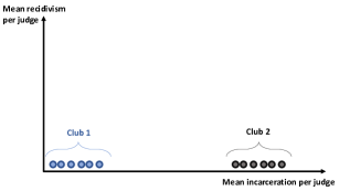
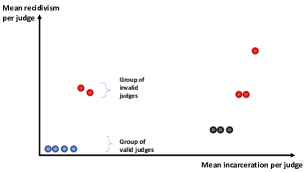
Figure 1: Illustration of the estimation approach

Note: The first step of the procedure (left graph) detects clubs with comparable propensity scores. This provides us with two clubs in the given example. The second step detects groups with comparable reduced form estimates of judge- (or IV-) specific mean outcomes and selects the largest groups within clubs as the validity set (right graph). After this two-step classification, pairing the largest groups across different clubs (or propensity score values) permits estimating the LATE.

We use the Agglomerative Hierarchical Clustering (AHC) algorithm of Ward (1963) to perform both steps of our procedure. In order to further improve the clustering, we also combine AHC with the clustering algorithm in regression via data-driven segmentation (CARDS, Ke, Fan, and Wu, 2015). We report the results of the CARDS approach in Appendix B.2. However, we cannot achieve any improvement using the CARDS approach compared to AHC. Furthermore, CARDS is not computationally efficient, while AHC is much faster and therefore, overall preferable. In a previous version of the paper, we also considered so-called Classifier-Lasso (Su, Shi, and Phillips, 2016) for the estimation of club identities. However, again we could not improve the results compared to AHC.

3.2 Club classification

The first step for estimating LATEs consists of detecting clubs of treatment propensity scores based on Assumption 4. We estimate club membership based on the Agglomerative Hierarchical Clustering (AHC) algorithm of Ward (1963). This method was first applied to the selection of valid instruments by Apfel and Liang (2021) in the context of over-identified parametric models where the number of valid instruments exceeds the number of regressors and plurality is fulfilled. Here, we instead use it for clustering the treatment propensity scores as a function of the instruments. We denote by $\mathcal{C}$ a partition into clusters with $C_{k}\in\mathcal{C}$ and by $\hat{\mathcal{C}}$ the estimated partition of the data. The true partition is denoted by $\mathcal{C}^{0}$. In the following, we provide a description of the algorithm, which is closely related to that given in Apfel and Liang (2021):

Algorithm 1.

Agglomerative Hierarchical Clustering

1. Input: Calculate the IV-specific propensity scores and the Euclidean distance between them, which is stored in a dissimilarity matrix.

2. Initialize: At the beginning, each propensity score is assigned to its own cluster and therefore, the total number of clusters at the initialization step is $J$.

3. Join: The two clusters which are closest in terms of their weighted squared Euclidean distance are merged into a new cluster. Formally, the weighted squared Euclidean distance is defined as $\frac{|C_{k}||C_{l}|}{|C_{k}|+|C_{l}|}||\bar{C}_{k}-\bar{C}_{l}||^{2}$, with $|C_{k}|$ denoting the number of propensity scores in cluster $k$ and $\bar{C}_{k}$ the arithmetic mean of propensity scores in cluster $k$.

4. Iterate: Repeat the joining step until all propensity scores are in one cluster.

We note that distinct weighing schemes in the Euclidean distance correspond to distinct objective functions to be minimized. We follow the classical approach in Ward (1963) and define the sum of within-cluster variance as objective function. As discussed in Apfel and Liang (2021), the results, however, do not rely on this specific choice of the dissimilarity metric. When running the algorithm, we obtain a path of $S=J-1$ steps, with clusters of size $|\hat{C}_{k}|\in\{1,...,J\}$ at each step. Note that each number of clusters, $K$, entails a different estimated partition $\hat{\mathcal{C}}(K)$.

To apply Algorithm 1 in practice, a central question is at which step one should stop the merging process of clusters. The penalty parameter to choose in this context is the number of clusters $K$. We propose the following procedure based on F-tests for equality of parameters to optimally select $K$. Starting with $K=1$, we test whether all of the propensity scores are equal. If the test rejects the null, we proceed to the step of the AHC with $K=2$ and test for equality of all propensity scores within each cluster (or club).

Algorithm 2.

Selecting number of clusters via F-test

1. Select a significance level $\alpha$

2. Set $K=1$

3. Testing: Perform an F-test at the significance level $\alpha$, with $H0:\,$ Propensity scores within any cluster are equal

4. Updating: If rejected, increase $K$ by 1

5. Iterate testing and updating until F-test does no longer reject $H0$.

The asymptotic F-statistic for the test applied in Algorithm 2 is defined as

$$(J-K)F(\hat{\mathbf{p}},\mathcal{C})=(\mathbf{R}(\mathcal{C})\hat{\mathbf{p}}-\mathbf{0}_{J})^{T}\left[s^{2}\mathbf{R}(\mathcal{C})(\mathbf{Z}^{T}\mathbf{Z})^{-1}\mathbf{R}(\mathcal{C})^{T}\right]^{-1}(\mathbf{R}(\mathcal{C})\hat{\mathbf{p}}-\mathbf{0}_{J}),$$ (13)

where $\mathbf{R}(\mathcal{C})$ is a hypothesis matrix with dimension $(J-K)\times J$. For the IV of the first club to be tested for equality, the matrix entry is 1 and for the remaining IVs it is zero, except for one other IV in the club, whose entry is -1. In this way, we test the equality of all coefficients. $\mathbf{0}_{J}$ is a $(J\times 1)$ vector of zeros. Under the $H0$, the test statistic follows a $\chi^{2}$-distribution with $J-K$ degrees of freedom.

After identifying clubs of IVs with comparable propensity scores, clubs with distinct propensity score values may be paired to obtain the first stage effect of the instrument on the treatment as the difference across club-specific propensity scores. In this context, one club of judge IVs in the pair may be considered as reference category and the other as focal category. Estimating the LATE within a club-pair can be based on the subsample which exclusively contains observations (court rulings) coming from either the reference judges or the focal judges in that pair. In this case, the club-pair-specific instrument can be defined as a dummy variable, which takes the value one whenever a defendant is assigned to one of the judges from the focal category and zero otherwise. This approach yields just-identified IV models for each club-pair (due to using subsamples with reference and focal judges), which we may consistently estimate by 2SLS under the satisfaction of the LATE assumptions.

One may also create multiple instruments within a club-pair based on individual judges in that pair and run a 2SLS regression using these instruments. More concisely, we can for instance consider all judges in the club with the lower propensity score as reference category and generate separate instrumental dummy variables for each judge in the focal category. Asymptotically, all pair-specific IV dummies must yield identical LATEs if the LATE assumptions as well as Assumption 4 on first-stage clusters hold, as they refer to the same complier population in terms of unobservables. Finding heterogeneous LATEs within club-pairs therefore points to a violation of the identifying assumptions, which motivates the procedure outlined in the next section. In contrast, LATEs that are based on distinct club-pairs refer to distinct complier populations and can for this reason differ under our heterogeneous treatment effect model.

3.3 Group classification

After clustering on the first-stage propensity score, any remaining heterogeneity in the LATE must come from the violation of one or several LATE assumptions outlined in Section 2.2. Put differently, if all judge-specific IVs constructed within a club-pair satisfy the LATE assumptions, then IV estimates based on the various judge IVs should yield comparable LATEs and tests of overidentifying restrictions in IV models should not reject. For instance, one may apply a Hansen-Sargan-type test to multiple IVs created from two paired clubs of homogeneous propensity scores. In classical parametric IV models which impose homogeneous treatment effects and do not rely on first-stage clustering for generating clubs, such tests may not only have power against violations of IV assumptions, but also against a violation of effect homogeneity. In our framework allowing for heterogenous treatment effects, however, the application of Hansen-Sargan-type tests within club-pairs tailors it to testing the LATE assumptions rather than functional form restrictions.

To allow for a violation of the LATE assumptions, we proceed to the second step of our procedure, a clustering approach for determining the validity set $\mathcal{V}$ as provided in Definition 1. To this end, we apply Algorithms 1 and 2 another time, but now for detecting groups within a club that are homogeneous in terms of reduced form estimates of judge-specific mean outcomes $r_{z}$. This requires first estimating the reduced form parameters by a linear regression of the outcome $Y$ on IV dummies for all judges (but no constant) within a club with homogeneous propensity scores. Therefore, the instrument $Z$ satisfies $Z\subseteq C^{k}$ in club $k$. Then, the identical cluster procedure as previously used for detecting first-stage clubs is applied to the reduced form estimates of $r_{z}$, in order to classify them into homogeneous groups. Finally, we select the groups with the largest number of instruments within a club as the validity set, relying on the plurality assumption introduced earlier.

We note that our procedure is not the only feasible approach for selecting true instruments in heterogeneous treatment effect models under the plurality assumption. As an alternative to selecting instruments within first-stage clubs based on the reduced form mean, one can also estimate all possible judge-pair-specific LATEs within a club-pair (or union) and group them by our clustering procedure. More concisely, for two first-stage clubs $a$ and $b$ containing $J_{a}$ and $J_{b}$ judges, respectively, there are $J_{a}\cdot J_{b}$ possible judge pairs for computing the LATE. We may apply the AHC algorithm to cluster the LATE estimates which are closest to each other in terms of weighted Euclidean distances. After each clustering iteration, we can extract the estimates in the largest cluster of estimates and verify their homogeneity based on a Hansen-Sargan-type test. In simulations (not reported), we found this approach to yield very similar results as our suggested procedure of clustering the reduced form means. For simplicity, we focus on the reduced form-based approach. One advantage of the latter approach is that it permits testing individual judge IVs rather than pairs of judges. This implies that for two first-stage clubs $a$ and $b$, the clustering method is based on only $J_{a}+J_{b}$ first stage estimates, rather than $J_{a}\cdot J_{b}$ LATE estimates when pairing the judges.

3.4 Post-classification estimation

Clustering first-stage clubs and reduced-form groups within clubs provides us with an estimate of clubs $\hat{\mathcal{C}}$ as well as the validity set $\hat{\mathcal{V}}$, which consists of the largest club-specific groups. Based on these estimates, we compute the LATE by the sample analog of equation (2) or equivalently, by 2SLS, using observations in the validity set that come from two different clubs (and thus, differ in terms of propensity scores).

More formally, we define $Z_{k}$ to be an aggregated instrument indicating whether a judge IV $z$ in estimated club $k$ belongs to the largest group of reduced form mean outcomes:

$$Z_{k}=\mathbbm{1}(z\in\hat{\mathcal{R}}_{max}^{k})\text{,}$$ (14)

where the subscript $max$ refers to the largest reduced-form group in first-stage club $k$. For two clubs $k$ and $k^{\prime}$ with distinct propensity scores, the LATE estimator exclusively using observations from the two largest groups in two clubs (such that an observation $i$ satisfies $i:z\in\hat{\mathcal{R}}_{max}^{k}\cup\hat{\mathcal{R}}_{max}^{k^{\prime}}$), denoted by $\hat{\beta}(\hat{\mathcal{R}}_{max}^{k},\hat{\mathcal{R}}_{max}^{k^{\prime}})$, then corresponds to

$$\hat{\beta}({\hat{\mathcal{R}}_{max}^{k},\hat{\mathcal{R}}_{max}^{k^{\prime}}})=\frac{\sum_{i:z\in\hat{\mathcal{R}}_{max}^{k},\hat{\mathcal{R}}_{max}^{k^{\prime}}}Z_{i,k,k^{\prime}}Y_{i}}{\sum_{i:z\in\hat{\mathcal{R}}_{max}^{k},\hat{\mathcal{R}}_{max}^{k^{\prime}}}Z_{i,k,k^{\prime}}D_{i}}$$ (15)

where the IV which sets observations to zero for members of one group and to one for members of the other group is

$$Z_{k,k^{\prime}}=\begin{cases}1\text{ if }z\in\hat{\mathcal{R}}_{max}^{k}\\ 0\text{ if }z\in\hat{\mathcal{R}}_{max}^{k^{\prime}}\end{cases}$$ (16)

We term such an estimator a group-pair IV estimator (GPIV).

3.5 Consistent classification and asymptotic normality

In the following, we prove that our procedure consistently classifies propensity scores and selects the validity set. Then, we go on to show that the IV-estimator using the selected groups is asymptotically normal. We first introduce estimands, which compare two clubs or groups

$$\beta(\mathcal{C},\mathcal{R},k,k^{\prime})=\frac{E(Z_{i,k,k^{\prime}}Y_{i}|z\in\mathcal{R}_{max}^{k}\bigcup\mathcal{R}_{max}^{k^{\prime}})}{E(Z_{i,k,k^{\prime}}D_{i}|z\in\mathcal{R}_{max}^{k}\bigcup\mathcal{R}_{max}^{k^{\prime}})},\textit{for k, k'}\in\{1,...,K\}$$ (17)

We have that $plim(\hat{\beta}({\hat{\mathcal{R}}_{max}^{k},\hat{\mathcal{R}}_{max}^{k^{\prime}}}))=\beta(\mathcal{C},\mathcal{R},k,k^{\prime})$. The estimand for the GPIV estimator which uses the correct club identities and validity set is

$$\beta(\mathcal{C}_{0},\mathcal{V},k,k^{\prime})=\frac{E(Z_{i,k,k^{\prime}}Y_{i}|z\in\mathcal{V}^{k}\bigcup\mathcal{V}^{k^{\prime}})}{E(Z_{i,k,k^{\prime}}D_{i}|z\in\mathcal{V}^{k}\bigcup\mathcal{V}^{k^{\prime}})},\textit{for k, k'}\in\{1,...,K^{0}\}$$ (18)

We call the corresponding estimator the oracle GPIV estimator for $k,k^{\prime}$. $K=K^{0}$ means that the number of clusters is equal to the true number of clubs. There could also be estimators with $K\neq K^{0}$. This GPIV estimator identifies the true underlying group-pair specific LATE, $\Delta(k,k^{\prime})=E[Y(k^{\prime})-Y(k)|v\geq V>v^{\prime}]$, i.e. $\hat{\beta}(\mathcal{C}_{0},\mathcal{V},k,k^{\prime})\overset{p}{\rightarrow}\Delta(k,k^{\prime})$ for $k,k^{\prime}\in\{1,...,K^{0}\}$. The following result will help establishing consistent classification.

Corollary 1.

The true partition is on the selection path
As $N_{z}\rightarrow\infty\,\,\forall z$ and $K=K^{0}$: $lim\,P(\hat{\mathcal{C}}(K)=\mathcal{C}^{0})=1$.

This follows directly from Lemma LABEL:lemma:SameClubFirst in the Appendix. The idea is that we start with $K=J$ and then merge only clusters which contain propensity scores from the same club. Only when all $p_{z}$ from each club are in a cluster respectively, the algorithm starts to merge clusters with members of different clubs.

Theorem 1.

Consistent classification
Let $\xi_{n}$ be the critical value for the F-test in Algorithm 2. Let $\hat{\mathcal{C}}$ be the partition selected from Algorithm 1 and Algorithm 2. Under Assumptions 4 and 6-8, for $\xi_{n}\rightarrow\infty$ and $\xi_{n}=o(n)$,

$$\underset{n\rightarrow\infty}{lim}P(\hat{\mathcal{C}}=\mathcal{C}^{0})=1.$$

This theorem shows that asymptotically, algorithms 1 and 2 correctly select the club identities, i.e. the correct partition $\mathcal{C}^{0}$. The next corollary states that the analogous algorithms for the maximal group selection inside each cluster will select the validity set.

Corollary 2.

Consistent group selection
Let $\xi_{n}$ be the critical value for the F-test in Algorithm 2. Let $\hat{\mathcal{R}}_{max}$ be the partition selected from Algorithm 1 and Algorithm 2. Under Assumptions 5-8, for $\xi_{n}\rightarrow\infty$ and $\xi_{n}=o(n)$,

$$\underset{n\rightarrow\infty}{lim}P(\hat{\mathcal{R}}_{max}=\mathcal{V})=1.$$

The proof of this theorem follows the ones of Theorem 1 in this paper and of Theorem 1 in Apfel and Liang (2021) closely and is hence omitted. The main difference is that the correct selection of the validity set does not rely on correctly assigning each judge to its group. As long as the invalid judges are not in the largest group, the algorithms still correctly select the validity set, even for cases where $K\neq K^{0}$. By theorems 1 and 2 we now have that as $n\rightarrow\infty$, $\hat{\mathcal{C}}=\mathcal{C}^{0}$ and $\hat{\mathcal{R}}_{max}=\mathcal{V}$ with probability approaching one. The next theorem states that the GPIV is asymptotically normally distributed.

Theorem 2.

Asymptotic normality
Under Assumptions 4 to 8, for $\xi_{n}\rightarrow\infty$ and $\xi_{n}=o(n)$,

$$\sqrt{n}(\hat{\mathbf{\beta}}(\hat{\mathcal{C}},\hat{\mathcal{R}},k,k^{\prime})-\Delta(k,k^{\prime}))\overset{d}{\rightarrow}N(0,\mathbf{V}_{k,k^{\prime}})$$ (19)

for all pairs $k,k^{\prime}$.

4 Simulation

We investigate the finite sample properties of our clustering and testing procedure in a simulation study consisting of two settings, with and without invalid judge IVs, where invalidity refers to a violation of the IV exclusion restriction. We consider three different sample sizes to analyze consistency.

4.1 Simulation design

We analyse settings with unbalanced panels, with $J=10$ judges. To determine the number of cases per judge we draw from a uniform distribution $Unif(3,5)$, multiply this value by 20, 60, or 100, respectively, and round the number to the next integer. We repeat this approach for all $J$ judges and construct dummy variables for each judge. Furthermore, we define the first-stage model for the treatment of an observation $i$ in the following way:

$$D_{i}=\mathbbm{1}(\mathbf{z}_{i}\cdot\bm{\pi}>V_{i})$$

where $\mathbf{Z}$ is the $(N_{z}\cdot J)\times J$ matrix of judge dummies and $\mathbf{z}_{i}$ is a row vector. $\bm{\pi}=(0.8,0.5,0.3)^{\prime}$ is the vector of first stage coefficients (or propensity scores) of the judge dummies. $V_{i}$ is the first-stage error and follows a uniform distribution, $V_{i}\sim Unif(0,1)$. In this setup we create three clubs with 4, 4, and 2 different judges per club, respectively.

To avoid the correlation between the steps of clustering and estimating the LATEs, we apply sample splitting. That is, we divide the cases per judge into a training and a test set. We use the training set to cluster the judges into clubs and apply the second step of the procedure to detect invalid judges. We use the groupings from this step to estimate the group-pair wise LATEs.

The outcome model is given by the nonlinear function

$$Y_{i}=(D_{i}\cdot 0.5+D_{i}\cdot U_{i}+\mathbf{Z}\gamma+U_{i})^{4}.$$

$U_{i}$ is the error in the outcome equation and modelled as $U_{i}=0.5\cdot V_{i}+W_{i}$, where $W_{i}=Unif(0,1)$ is a uniform random variable which is independent of $V_{i}$. As the first-stage error affects the error in the outcome equation, the treatment is endogenous, which motivates the application of our IV approach. $\bm{\gamma}$ is a vector of direct effects of the instruments on the outcome. Therefore, a nonzero entry $\bm{\gamma}$ implies a violation of the exclusion restriction for the related judge dummy and thus, of one of the LATE assumptions. We define two different settings regarding the invalidity of the judges, to be able to identify the accuracy of the LATEs in both stages, before and after the identification of the invalid IVs. In the first setting we set $\bm{\gamma}=(0\bm{i}_{10})$. This allows us to investigate the club assignment in detail. In the second setting, we set $\bm{\gamma}=(0.5,0\bm{i}_{3},0\bm{i}_{2},0.4,0.6,0\bm{i}_{2})$, so that in club 1, three judges are valid and one is invalid and hence majority is still fulfilled, in club 2, two judges are invalid and two valid, and hence plurality is fulfilled, but majority is violated, and in club 3 all judges are valid. While we focus on violations of the exclusion restriction to investigate the finite sample performance of our method, we notice that one could also consider violations of other LATE assumptions, namely treatment monotonicity or random IV assignment.

We report the following statistics for the simulations. Under $\#clubs$, we report the mean number of clubs, under $\#corr$ we report the fraction of times the correct number of clubs has been selected. We report the estimated LATEs for each pair comparison, when the number of clubs selected is the true number of clubs ($1-2$, $1-3$, $2-3$). For comparison we also report the true (or oracle) LATE. This fully informed estimator can be computed directly from the data generating process of our simulation. We take the average of Hansen p-values for each repetition (over pair-comparisons) and then average these means over repetitions ($Hansen$ $p$). We also calculate the probability ($Power$) of detecting a non-zero effect by testing the beta coefficients against zero. Respectively we calculate the average coverage rate ($Cover$), by testing whether the estimated 95 percent confidence intervals contain the true LATE. We simulate the true LATE by calculating the mean of 5000 oracle estimates, estimated using data independent from the one used to illustrate the selection and estimation procedures.

We report the mean normalized mutual information (NMI), which is an indicator for the quality of the clustering, as used in Ke et al. (2015) and Ana and Jain (2003). The NMI is defined for the comparison of a clustering $\mathcal{C}$ and the oracle clustering $\mathcal{C}_{0}$:

$$\mathrm{NMI}(\mathcal{C},\mathcal{C}_{0})=\frac{I(\mathcal{C};\mathcal{C}_{0})}{[H(\mathcal{C})+H(\mathcal{C}_{0})]/2}$$

where $I(\mathcal{C};\mathcal{C}_{0})=\sum_{k,j}\left(\left|C_{k}\cap C_{0j}\right|/\right)\log\left(\mid C_{k}\cap\right.\left.C_{0j}|/|C_{k}||C_{0j}\mid\right)$ is the mutual information between the two clusterings and $H(\mathcal{C})=-\sum_{k}\left(\left|C_{k}\right|/\right)\log\left(\left|C_{k}\right|\right)$ is the entropy of $\mathcal{C}$. The NMI takes values between 0 and 1, with larger NMIs indicating more similar clusterings and a value of 1 meaning that they are equal.

In a separate table, we report the results for the second-step AHC: the average of the fraction of valid IVs detected ($ValDet$) and of invalid IVs detected ($InvDet$). Further we also report the percentage of repetitions in which all valid and invalid IVs were correctly identified ($CorVal$) and again $Hansen$ $p$, $Power$, $Cover$ as well as the estimated LATEs.

4.2 Simulation results

We first consider a setting without invalid IV dummies, implying that all entries of $\gamma$ in the outcome equation are equal to zero, and run 1000 Monte Carlo simulations. Table 4.2 reports the mean OLS and 2SLS coefficient estimates and standard error, for the three sample size settings. In the smallest sample size setting (20) the OLS estimate is 18.87 with 1.02 as a standard error. The 2SLS coefficient estimate is slightly higher at 20.31 and 1.48 as standard error. We observe almost the same coefficient estimates for the two larger sample settings, with considerably lower standard errors for OLS and 2SLS. The F-statistic on the instruments, in all settings, indicate that judge dummies are strong instruments for incarceration.

Table 1: Mean OLS and 2SLS

Setting	Method	Est	SE	F-statistic
20	OLS	18.87	1.02
	2SLS	20.31	1.48	74.63
60	OLS	18.91	0.59
	2SLS	20.38	0.86	219.13
100	OLS	18.90	0.46
	2SLS	20.38	0.67	363.87

Note: Setting: number of cases per judge ($Unif(3,5)\times(20,60,100)$); Method: OLS regression, two-stage least-squares regression; Est: estimates of incarceration on recidivism, using judge dummies for 2SLS; SE: robust standard errors; F-statistic: First-stage F-statistic, testing joint relevance of the instruments.

Table 4.2 shows the classification results after the first step of our method, for both settings, with and without invalidity. In the first step, we aim at detecting clubs of treatment propensity scores based on Assumption 4. We estimate club membership based on our algorithms 1 and 2. For comparison, we also report the oracle LATE estimator. In Table 4.2 we first have a look at the setting without any invalid IVs. Column 5 ($\#corr$) shows that using AHC we find the right number of clubs, respectively, in 33 percent, 95 percent, and 99 percent of the repetitions, based on the different sample sizes. Increasing the sample size greatly improves the clustering performance. The average of the Hansen p-value is considerably above any conventional significance level, indicating we cannot find evidence for invalid instruments. Therefore, the second classification step (based on the reduced form parameters) is not necessary. The CI coverage is close to its nominal level for all sample sizes.

In the setting with invalid IVs we observe a comparable performance, when it comes to the identification of the right number of clubs. However, the Hansen p-value is always below the 0.05 significance level, indicating a high rate of rejections of the Null. There are two possible reasons that lead to a rejection of the Hansen test: effect heterogeneity and invalidity. By classifying the judges into clubs with the same incarceration rate, we can rule out effect heterogeneity as potential cause of a rejection of the Hansen test. Therefore, if it still rejects after classifying judges into groups, the only reason left for rejecting is the presence of invalid judges.

Table 2: Simulation: First step - club allocation.

Note: Mean results after the first step of the procedure (detecting clubs with comparable propensity scores). Setting: number of cases per judge ($Unif(3,5)\times(20,60,100)$); Invalidity: no: $\gamma=(0i_{10})$, yes: $\gamma=(0.5,0i_{3},0i_{2},0.4,0.6,0i_{2})$; Method: Oracle: estimator that uses group and club identity information, AHC: agglomerative hierarchical clustering; $\#clubs$: mean number of clubs; $\#corr$ percentage of iterations in which the correct number of clubs has been selected; Hansen p: mean of p-values of Hansen-test from an over-identified specification; Power: fraction of confidence intervals that do not include zero; Cover: fraction of confidence intervals containing the true effect; NMI: normalized mutual information.

To address invalidity, we apply the second step of our IV selection procedure. In Table 4.2 we present the classification results after the second stage of our procedure, that is applied to identify and eliminate invalid judges from the estimation. We apply AHC in both steps of the procedure, using the classification results shown in Table 4.2.

After applying the second step, Table 4.2 shows that the average of the Hansen p-value is considerably above any conventional significance level for all methods, indicating we no longer find evidence of invalid instruments. The power is close to 1, depending on the sample sizes, while the Coverage is between 0.76 and 0.91 for AHC. Respectively 97 to 99 percent of the valid IVs have been correctly detected ($ValDet$). The fraction of correctly identified invalid IVs ($InvDet$) is slightly lower at respectively 69, 87, and 96 percent. In total, again respectively for the sample sizes, in 33, 68, and 90 percent of the repetitions AHC identified all valid and invalid IVs correctly ($CorVal$). An NMI very close to 1 also indicates that the correct grouping has been retrieved in many cases.

Table 3: Simulation: First and second step - club allocation and identification of invalid judges.

Note: Mean results after the first and second step of the procedure (detecting clubs with comparable propensity scores and eliminating invalid judges) for $\gamma=(0.5,0i_{3},0i_{2},0.4,0.6,0i_{2})$. Setting: number of cases per judge ($Unif(3,5)\times(20,60,100)$); Method: Oracle: estimator that uses group and club identity information, AHC: agglomerative hierarchical clustering; Hansen p: mean of p-values of Hansen-test from an over-identified specification; Power: fraction of confidence intervals that do not include zero; Cover: fraction of confidence intervals containing the true effect; ValDet: fraction of valid IVs selected as valid; InvDet: fraction of detected, invalid IVs; CorVal: percentage of iterations in which all valid and invalid IVs were identified correctly.

In Table 4.2 we report the respective LATE estimates, averaged over all repetitions (in which the correct number of clubs was found). In the setting without invalidity, the estimated LATEs, using AHC, are extremely close to the oracle LATEs and the SE decrease with increasing sample size. In the setting with invalidity, we first evaluate the performance of LATE estimates after only the first (club assignment) step, without trying to detect invalid judges. As expected, given that invalid judges are still present in the estimation, mean coefficient estimates are far from the oracle estimates, irrespective of sample size. Applying the second, group selection step of the method, however, dramatically improves our estimation and now the estimates from our method and the oracle estimates are very close. With a small sample, when for each judge there are only 60 to 100 observations per judge, the variance can be very large, but the performance clearly improves in the medium sample setting, with 180 to 300 observations and it is best in the largest sample setting.

Table 4: Simulation: LATEs.

Note: Setting: number of cases per judge ($Unif(3,5)\times(20,60,100)$); Invalidity: no: $\gamma=(0i_{10})$, yes: $\gamma=(0.5,0i_{3},0i_{2},0.4,0.6,0i_{2})$; Method: Oracle: estimator that uses group and club identity information, AHC: agglomerative hierarchical clustering; Stage: results after the first (detecting clubs with comparable propensity scores) or second (detecting clubs with comparable propensity scores and eliminating invalid judges) stage; 1-2, 1-3, 2-3: Group-wise LATE estimates of incarceration on recidivism, using judge IVs. SE: robust standard errors

Overall, these simulations indicate that our method delivers reliable results, retrieving clubs and groups that fulfil the LATE assumptions and they indicate that the oracle properties shown earlier on in the paper indeed hold. Additionally, the methods can be expected to perform well already with samples of medium size. We expect that performance not only improves with the number of observations, but also with increasing value of violations, increasing degree of separation among propensity scores and decreasing error variance.

5 Application

5.1 Assessing the effect of incarceration on recidivism

In recent years, several studies have addressed the question whether incarceration affects the likelihood of recidivism (future criminal behavior) or, in other words, whether sentencing offenders to prison affects the likelihood of them relapsing into criminal behavior. Incarceration could either decrease the likelihood of recidivism if prisons help rehabilitate offenders and reintegrate them into society. If, however, the time in prison integrates them into criminal networks or leads to a loss of human capital, incarceration might increase the likelihood of recidivism. In order to answer this question, authors typically aim at estimating the following empirical model:

$$Y_{jc}=D_{jc}\beta+\mathbf{x}_{jc}\theta+\varepsilon_{jc}$$ (20)

where $Y_{jc}$ denotes the outcome, an indicator for recidivism, i.e. re-indictment or re-incarceration in a certain time window after conviction, $j$ is the judge-index and $c$ is the case-index. $D_{jc}$ is the treatment variable with the coefficient of interest $\beta$, indicating whether a judge has sentenced the convict to a term of imprisonment or has decided for a non-prison sentence, such as probation. $\mathbf{x}_{jc}$ are observed covariates potentially affecting the probability of recidivism, with the coefficient vector $\theta$. Nagin, Cullen, and Jonson (2009) suggest to use prior record, offence type, age, race and sex as key control variables. $\varepsilon_{jc}$ reflects unobserved characteristics affecting the outcome.

Estimating equation (20) by OLS is generally biased and inconsistent if the association between outcome and right-hand side variables is non-linear and/or unobserved confounders jointly affect $D$ and $Y$ even after controlling for $X$. For instance, the judge might have information (not available to the researcher) about the defendant’s previous offenses or possible addictions, which may simultaneously influence the judge’s sentencing and the likelihood of recidivism. Likewise, the sentence may be influenced by the defendant’s behavior in court, which in turn may shed light on the defendant’s potential to recidivate. In order to address this issue of unobserved confounders, several studies have leveraged the fact that in some judicial systems cases are randomly assigned to judges whose use of prison sentences varies systematically. They have considered dummies for being assigned to a particular judge or the incarceration rate by judge as instrumental variables. Following this literature, we also use a set of judge IV dummies.

Earlier evidence on the effect of imprisonment is mixed but studies that find crime-increasing and null effects are in the majority. Loeffler and Nagin (2021) provide a review of 13 published IV-based studies on the effect of incarceration on recidivism concluding that those based on data from U.S. courts mainly find either an insignificant or a significant recidivism-increasing effect. It appears that U.S. prisons are ineffective in terms of rehabilitation and resocialization, and thus do not serve to fight crime beyond general deterrence effects. In contrast, a study by Bhuller, Dahl, Løken, and Mogstad (2020) finds that incarceration in Norwegian prisons has a significant recidivism-reducing effect and a positive impact on employment, pointing to considerable heterogeneity in the effect of incarceration across regions, possibly due to differences in prison infrastructure and support services, such as labor market training opportunities.

Effect heterogeneity can also arise within the same institutional context, in that defendants sentenced to prison by different judges generally differ in their background characteristics (such as personality traits) and these in turn can influence the effect of incarceration. For this reason, the LATE, i.e. the effect of incarceration on recidivism among individuals who would be incarcerated under a stricter but not a more lenient judge might generally differ across distinct pairs of judges (or relatedly, distinct propensities of incarceration). Such effect heterogeneity would be masked when applying 2SLS simultaneously to all judge IVs, because the 2SLS estimator is a weighted combination of just-identified IV estimators, which in turn estimate LATEs. This is one motivation for using our approach.

Further, the instruments might fail to satisfy the identifying assumptions 1 to 3. For instance, judges could differ in terms of their use of alternative measures to imprisonment, such as electronic monitoring (Loeffler and Nagin, 2021), which would violate the exclusion restriction postulated in Assumption 1. Further, the IVs might violate Assumption 2, requiring monotonicity of the treatment in the instrument, see for instance the discussion in Frandsen, Lefgren, and Leslie (2023). Depending on how different judges weigh the individual aspects of a case, a rather stringent judge with a relatively high rate of prison sentences could refrain from incarcerating a particular defendant, who would have been imprisoned by a judge with a lower incarceration rate. i.e. their (potential) sentences could contradict the judges’ order of (average) severity. Such a situation entails the existence of defiers and thus a violation of weak monotonicity of the treatment in the instrument.

To nevertheless consistently estimate the LATEs of interest, we invoke the existence of clubs of judges with a similar propensity to incarcerate, as well as plurality, such that the largest group of judges constitutes IVs fulfilling the LATE assumptions. The cluster assumption appears realistic as long as judges can be plausibly categorized into a limited number of judge types, each with a distinct rate of prison sentences. As an example, Green and Winik (2010) exploit variation in judicial calendars, where it could be the case that judges assigned to the same calendar affect each other’s decisions. Moreover, some judges have moved between courts and reappear in the data with different judge IDs. Judges might have been educated and practiced at the same institutions, establishing cultures of higher or lower use of prison sentences. Moreover, in the US, different severity of judges might reflect judges’ allegiance to political parties.

5.2 Data

The model developed in Section 2 is applied to a data set of offenders in the U.S. state of Minnesota, which is composed of data from two primary sources: the first one is an extract from the Minnesota Judicial Branch case database containing information on the offender, including their full name, date of birth and place of residence, for all criminal cases from 2009 to 2020; the second source is a data set from the Minnesota Sentencing Guidelines Commission on all adult offender cases in Minnesota between 2001 and 2017, with information on the type and severity of the offense as well as the judge hearing the case. We link these two datasets using the case number as identifier in order to obtain a data set with years ranging from 2009 to 2017 on all criminal offense cases that includes information on offender, judge, offense and conviction.

For each offender in our data set, we identify all criminal cases in Minnesota in which they were involved between 2009 and 2017, using the offenders’ full names and dates of birth as identifiers. Despite also having information on the offenders’ place of residence, we do not include this information for identifying recidivism in order to account for changes of residence, which occur frequently, especially after returning from jail or prison. This way, we accept the low risk of incorrectly linking the cases of two individuals with the same name and date of birth, while reducing the risk of not detecting recidivism. In addition, we cannot detect recidivism if an offender committed a crime in another state, has moved to another state/country or has changed his or her name.

For estimating the effect of incarceration on offender recidivism, we consider recidivism within three years of sentencing as the outcome. Therefore, in order to observe the three-year post-conviction period of every offender, we must reduce our dataset to the years 2009 to 2014. According to the Minnesota Order for Assignment of Cases, all criminal cases in Minnesota are randomly assigned to a judge having jurisdiction in the county in which the crime is tried. After being assigned to a case, a judge in active service must preside over that case until its resolution, i.e., random judge assignment, as required for our IV approach, is guaranteed by Minnesota state case assignment rules. Senior judges, however, are permitted to opt out from hearing a case. We therefore remove all cases heard by a senior judge in order to ensure random judge assignment. Then, although the vast majority of judges in Minnesota remain in one and the same court throughout their tenure, there are some judges in the sample that have changed court during our observation period. These judges are assigned a different ID for each court such that the terms at different courts are treated as if belonging to different judges, in order to account for differences in county crime profiles, which in turn are reflected in the judges’ sentencing practices.

To ensure that the vast majority of offenders have been able to re-offend in the data within the three years following sentencing, i.e., are not in prison for the entire three years during which we observe potential recidivism, we need to reduce the data set to minor crimes. An analysis of the recidivism effect based on the entire dataset would require strict control for crime and offender profiles in order to avoid bias in the estimated effect caused by the inclusion of observations for which recidivism is highly unlikely due to long-term incarceration. At the same time, including offenses that result in a long prison sentence would not improve the quality of the estimator for the recidivism effect. Recent studies on the effect of incarceration have reduced their datasets based on different rules: Loeffler (2013) have concentrated on cases of the three lowest charge classes, Green and Winik (2010) on drug offenses. We follow Bhuller et al. (2020) by reducing the dataset based on the sentence lengths that an independent institution - in our case the Minnesota Sentencing Guidelines Commission - recommends for each observed offense given the type of crime, the severity of the offense and the offender’s criminal history. We reduce our dataset to cases with presumptive sentences of up to three years (a detailed list of the included offenses can be found in Appendix D.5). The resulting sample contains 48,849 cases involving 38,874 unique offenders. Only some 10 percent of the offenses in our sample did not result in incarceration.

Some 82 percent of the offenses in the final dataset have resulted in a sentence of up to one year in county jails, while in about 14 percent of the observed cases, offenders were sentenced to one to two years in state prison, meaning in 96 percent of the cases offenders had at least one year after their official release date to recividate. In only some 0.9 percent of the cases the offender was convicted to three or more years in state prison. Given that usually only two-thirds of a sentence are served in prison and the rest is on probation, the share of offenders having at least one year to recidivate is even higher than 96 percent.

5.3 Descriptive Statistics

Table D.4 in Appendix D.1 provides some descriptive statistics for our data, namely the mean of outcome and covariates in the total sample, as well as among those offenses resulting in a prison or jail sentence ($D=1$) and those that are not sanctioned with a prison or jail sentence ($D=0$). The descriptive statistics suggest that the distribution of prison/jail sentences differs not only in terms of crime type but also in terms of the offender’s race and gender. The proportion of cases that resulted in a prison or jail sentence is lower among white or Hispanic offenders than among offenders of other races and higher among men than among women. The share of property crimes sanctioned with incarceration is smaller than that of crimes against persons, drug crimes, weapon offenses and sex offenses. The table also shows that the severity of crimes and the likelihood of incarceration are positively correlated, where the variable “Severity” is an indicator for the seriousness of a crime as defined by the Minnesota Sentencing Guidelines Commission, ranging from low (Severity = 1) to high (Severity = 11).

5.4 Main analysis

We restrict the data to judges that heard at least 300 (results for 200 in D.3) randomly assigned cases between 2009 and 2017 and, in addition, to cases tried in counties where no fewer than two of these judges are stationed in any given year. The resulting samples contain respectively 11,219 cases.

We start with our first-step AHC and choose the significance level for the F-test as 0.1/log(N). In table 5.4, we show the results of the first stage clustering, for the sample with at least 300 cases per judge. We first partial out the controls from the outcome, treatment and the IVs. We then run the first-stage regression of the treatment (imprisonment) on all judge dummies. With that we get four clubs, of sizes 1, 3, 10, 11. We exclude the singleton club since the second stage selection would be pointless with a singleton club and we cannot be sure the judge is valid. The other propensity score means lie between 0.56 and 0.77.

Table 5: First-stage clubs, 300

Club	Mean	Nr
1	0.77	11
2	0.72	10
3	0.56	3
4	0.07	1

Note: Clustering results when minimum case count per judge is 300.

In Table 6 we run an OLS regression and a first baseline IV estimation, where we use judge dummies as instrumental variables. This IV approach is close to the approach by Green and Winik (2010) who use dummies for judicial calendars as instruments. We include race-, gender-, offense-type, year-dummies, severity, age, the squares of the latter two and race-gender interaction dummies. In practice, we partial these controls out of the outcome and the treatment variable. The OLS estimate is 0.06 and it is estimated with precision. The 2SLS estimate is 0.03, but it is insignificant, with an F-statistic at 76.50. The results of the baseline OLS and 2SLS estimations are in line with the IV literature on the effect of incarceration on recidivism (see e.g. Loeffler and Nagin, 2021).

The three further columns in Table 6 show the estimates for the pairwise comparisons between the three remaining clubs. In Panel A we do not run an IV selection, but use all of the judges within the clubs to build an IV which compares two clubs. The coefficients range from -0.10 to 0.20. The number of judges involved here lies between 13 and 21. F-statistics are mostly high and range between 64 and 175. A red flag is that even though we found different estimates with relevant first stages, the tests of overidentifying restrictions still reject clearly, with p-values close to zero for two of the three comparisons.

If we look for the largest group of reduced form coefficients and reduce the number of IVs further via our second-step AHC, we slightly increase the first-stage F-statistics, which are between 68 and 176. For two of the three clubs the Hansen-Sargan tests now do not reject any longer at any conventional significance level. The estimates again range from -0.10 to 0.50. The estimate for the comparison between club 1 and club 2 is highly significant.

Table 6: Effect of Imprisonment on Recidivism, 300

	OLS	2SLS	1-2	1-3	2-3
Panel A: Post Club Clustering
D	0.06	0.03	0.2	-0.02	-0.1
	(0.01)	(0.03)	(0.2)	(0.09)	(0.1)
J			21	14	13
N	11219	11219	4605	3290	2699
P		0.00	0.00	0.00	0.74
F		76.50	64.61	175.13	90.01

Panel B: Post Valid IV Selection
D			0.5	0.06	-0.1
			(0.2)	(0.09)	(0.1)
J			19	12	13
N			4298	2983	2699
P			0.53	0.02	0.74
F			68.75	176.32	90.01
Note: Sample restricted so that minimum number of cases per judge is 300. Cluster-robust standard errors in parentheses. Significance level in testing procedure: 0.1/log(N). D: coefficient for LATE estimate when comparing judge clubs or groups as detailed in top line. Panel A: Results after club-clustering, without valid IV selection, Panel B: Results after valid IV selection. J: Number of judges, N: number of observations, P: p-value of Hansen-test from an over-identified specification.

The first-stage clustering, as well as the validity set selection via clustering inside each club is presented in figure 2. We can see that there are three clusters of propensity scores with the lowest and smallest one separated most clearly from the other two. Judge-specific propensity scores, ordered by mean propensity score are also shown in figure D.2 in the Appendix, along with their confidence interval. In the rightmost club, two judges are selected as invalid and their reduced form appear to be clear outliers as compared to the $r_{z}$ of the remaining judges.

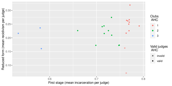
Figure 2: Reduced-form clustering

Note: Minimum number of cases per judge: 300. On vertical axis: mean outcomes per judge. Crosses denote judges selected as invalid, dots denote the selected validity set. Different colors denote different clubs.

The key takeaway of this application is that our method can discover different LATEs from a large set of IVs and can provide a list of LATEs that would otherwise be collapsed into a single 2SLS estimate. Using the second-step AHC we find subsets of IVs in the club-pairs that seem more likely to fulfil the exclusion restriction. Using the first-step AHC, we can find different clubs of propensity scores which yield very high first-stage F-statistics. Whether there is a monotonously increasing effect of the disaggregation of the 2SLS estimate into several LATEs on the first-stage F-statistic is unclear and is left for future research. Moreover, one might think about even more flexible ways to control for observables, such as through random forests or other machine learning methods.

5.5 Additional analyses

In the Appendix, we have added two additional exercises to this application. First, we have repeated the analysis, but now looking at judges with at least 200 cases. When doing this, we find five clusters, of which one singleton cluster (Table D.3 and Figure D.3). Invalid judges are now found in two of the clubs (D.4). When inspecting pairwise LATEs, qualitative results are similar to before in that the positive 2SLS estimate seems to be driven by a few positive, large and significant LATEs. In section D.4, we tackle the problem of controlling for observed covariates in an alternative way, by considering a subset of the data that is similar in terms of observables.

6 Conclusion

In this paper, we proposed a method based on hierarchical clustering for (i) estimating grouped LATEs under the condition that multiple instruments have the same firsts stage effect on the treatment and (ii) detecting instruments which satisfy the LATE assumptions, under the plurality condition that those assumptions hold for a relative majority of instruments with the same first stage. The method first groups instrument values based on their treatment propensity scores given the instrument and then groups the reduced form estimates (the mean outcomes given the instruments) within groups of propensity scores to determine the largest cluster of instruments as the one satisfying the LATE assumptions. This approach consistently selects clusters of identical first stages (and thus, complier groups) and of valid instruments to estimate the grouped LATEs under certain regularity conditions. Simulation results suggested a decent finite sample performance of our method even under a relatively moderate number of observations per instrument. Finally, we applied the procedure to assess heterogeneous effects of incarceration on recidivism when using randomly assigned judges as (binary) instruments, where it appears likely that the LATE assumptions fail for multiple judges. As a possible direction for future research, our method could also be extended to settings with non-binary instruments, like Mendelian randomization, where genetic markers are considered as potential instruments.

Appendices

A Methodological Appendix

A.1 Additional assumptions

To demonstrate that the algorithm covers the true partition, the following additional high-level assumptions are introduced:

Assumption 6.

Error structure

Let $\mathbf{w}_{i}=(u_{i}\quad\varepsilon_{i})^{\prime}$. Then, $E(\mathbf{w}_{i})=0$ and $E[\mathbf{w}_{i}\mathbf{w}_{i}^{\prime}]=\left(\begin{array}[]{cc}\sigma_{u}^{2}&\sigma_{u,\varepsilon}\\ \sigma_{u,\varepsilon}&\sigma_{\varepsilon}^{2}\end{array}\right)=\bm{\Sigma}$ with $Var(u_{i})=\sigma_{u}^{2},\quad Var(\varepsilon_{i})=\sigma_{\varepsilon}^{2}\quad Cov(u_{i},\varepsilon_{i})=\sigma_{u,\varepsilon}$ and the elements of $\bm{\Sigma}$ are finite. where $\varepsilon_{i}=D_{i}-E(D_{i}|Z=z)$ and $u_{i}=Y_{i}-E(Y_{i}|Z=z)$. The next assumption invokes the satisfaction of specific laws of large numbers.

Assumption 7.

$\frac{1}{\sum_{z=1}^{J}N_{z}}\mathbf{Z}^{\prime}\mathbf{Z}\overset{P}{\rightarrow}E(\mathbf{z}_{i}\mathbf{z}_{i}^{\prime})=\mathbf{Q}\text{ with }\mathbf{Q}$ a finite and full rank matrix and

$\frac{1}{N_{z}}\sum\limits_{i=1}^{n}D_{i}\mathbbm{1}(Z_{i}=z)\overset{P}{\rightarrow}E(D_{i}|Z_{i}=z)\forall z$ Denote $\mathbf{Z}$ a matrix including all judge dummies and $\mathbf{z}_{i}$ as the $J\times 1$ observation vector. By Assumption 7, the IV-specific average converges in probability to the conditional expectation of the treatment. In our empirical setup, the IVs are mutually exclusive dummies and hence the matrix product $\frac{1}{\sum_{z=1}^{J}N_{z}}\mathbf{Z}^{\prime}\mathbf{Z}$ is a diagonal matrix with entries $\frac{N_{z}}{\sum_{z=1}^{J}N_{z}}$, the number of unit observations for each IV. As the inverse of this is the diagonal matrix with entries $\frac{\sum_{z=1}^{J}N_{z}}{N_{z}}$, assuming that it is invertible is equivalent to assuming that as the number of cases for each judge goes to infinity, $N_{z}\rightarrow\infty$, the fraction of overall cases and judge-specific cases converges to a constant, $\frac{N_{z}}{\sum_{z=1}^{J}N_{z}}\rightarrow c$. Furthermore, we assume that a central limit theorem (CLT) holds such that

Assumption 8.

$\frac{1}{\sqrt{n}}\mathbf{Z}^{\prime}\mathbf{w}\overset{d}{\rightarrow}N(0,\mathbf{\Sigma}\otimes\mathbf{Q})$.

A.2 Proofs

A.2.1 Proof of Corollary 1

Here, we prove that $\mathcal{C}^{0}$ is on the selection path, that is for some $K$, Algorithm 1 assigns judges to their respective clubs. To show this, we first establish a Lemma from which correct assignment follows. The proof of this Lemma is very close to the one in Apfel and Liang (2021), but we reproduce it here to suit the setting and notation of the first-stage propensity scores.

Lemma 1.

Let $q$ and $q^{\prime}$ denote two clusters such that all propensity scores in the two clusters both satisfy $p_{z}\in C_{k}$ (i.e. the propensity scores in the two clusters belong to the same single club). Let $q^{\prime\prime}$ be a different cluster s.t. $\exists p_{z}:p_{z}\in\hat{C}_{q^{\prime\prime}}$ and $p_{z}\in C_{k^{\prime}}$ but $k^{\prime}\neq k$ (i.e. there is at least one propensity score in this cluster which does not belong to the club from which the previous two clusters come). Under Assumptions 7 and 4, as $N_{z}\rightarrow\infty\,\forall z$, clusters $q$ and $q^{\prime}$ are merged with probability converging to 1.

We subsequently demonstrate on a high level that the probability that an estimated cluster $\hat{C}_{q}$ with elements from the true club $C_{k}$ is merged with another estimated cluster with elements from the same club $\hat{C}_{k}$ goes to 1. The proof closely follows the one in Apfel and Liang (2021) and is divided into three parts for proving the subsequent statements:

1. The means of clusters which include propensity scores from the same club also converge to the same value as each propensity score in the club.

2. The algorithm merges the two clusters that have minimal distance.

3. Clusters with propensity scores from the same club have a distance of zero and clusters with propensity scores from more than one club have a non-zero distance, with the probability going to one.

Proof.

Part 1: Consider

$$\begin{split}z,z^{\prime}\in C_{k}\,\quad z^{\prime\prime}\in C_{k^{\prime}}\,\quad k\neq k^{\prime}.\\ \end{split}$$

Under Assumption 7 and 4, it follows that

$$\begin{split}plim(\hat{p}_{z})=plim(\hat{p}_{z^{\prime}})=p_{k}\\ plim(\hat{p}_{z^{\prime\prime}})=p_{k^{\prime}}\end{split}$$ (A.1)

Let $\hat{C}_{q}$ and $\hat{C}_{q^{\prime}}$ be estimated clusters with propensity scores from the same club: $\hat{C}_{q}$, $\hat{C}_{q^{\prime}}\subset C_{k}$ and $\hat{C}_{q^{\prime\prime}}\subset C_{k^{\prime}}$. Let $\bar{\hat{C}}_{k}$ denote the arithmetic mean of the propensity scores in an estimated cluster.

$$plim\,\,\bar{\hat{C}}_{q}=\frac{\sum\limits_{\hat{p}_{z}\in C_{k}^{0}}\hat{p}_{z}}{|\hat{C}_{q}|}=\frac{|\hat{C}_{q}|p_{k}}{|\hat{C}_{q}|}\text{ where }\hat{C}_{q}\subset C_{k}^{0}$$ (A.2)

and hence plim    ¯^C_q = p_k^0 .

Part 2: Consider the case that the algorithm decides whether to merge two estimated clusters, $\hat{C}_{q}$ and $\hat{C}_{q^{\prime}}$, containing propensity scores from the same club, or to merge two estimated clusters containing propensity scores from more than one underlying club, $C_{q}$ and $C_{q^{\prime\prime}}$. The two clusters which are closest in terms of their weighted Euclidean distance are merged first. Hence, we need to consider the distances between $C_{q}$ and $C_{q^{\prime}}$, $C_{q}$ and $C_{q^{\prime\prime}}$, as well as $C_{q^{\prime}}$ and $C_{q^{\prime\prime}}$.

$C_{q}$ is merged with a cluster with elements of its own club $C_{k}^{0}$ iff $\frac{|C_{q}||C_{q^{\prime}}|}{|C_{q}|+|C_{q^{\prime}}|}||\bar{\hat{C}}_{q}-\bar{\hat{C}}_{q^{\prime}}||^{2}<\frac{|C_{q}||C_{q^{\prime\prime}}|}{|C_{q}|+|C_{q^{\prime\prime}}|}||\bar{\hat{C}}_{q}-\bar{\hat{C}}_{q^{\prime\prime}}||^{2}$. Therefore, the following two are equivalent

$$lim\,P(C_{q}\cup C_{q^{\prime}}=C_{q,q^{\prime}}\subseteq C_{k}^{0})=1$$

$$\Leftrightarrow\quad lim\,P(\frac{|C_{q}||C_{q^{\prime}}|}{|C_{q}|+|C_{q^{\prime}}|}||\bar{\hat{C}}_{q}-\bar{\hat{C}}_{q^{\prime}}||^{2}<\frac{|C_{q}||C_{q^{\prime\prime}}|}{|C_{q}|+|C_{q^{\prime\prime}}|}||\bar{\hat{C}}_{q}-\bar{\hat{C}}_{q^{\prime\prime}}||^{2})=1$$ (A.3)

where $C_{q,q^{\prime}}$ is the merged cluster.

Part 3: Our objective is to prove (A.3). We can then prove $lim\,P(\frac{|C_{q}||C_{q^{\prime}}|}{|C_{q}|+|C_{q^{\prime}}|}||\bar{\hat{C}}_{q}-\bar{\hat{C}}_{q^{\prime}}||^{2}<\frac{|C_{q^{\prime}}||C_{q^{\prime\prime}}|}{|C_{q^{\prime}}|+|C_{q^{\prime\prime}}|}||\bar{\hat{C}}_{q^{\prime}}-\bar{\hat{C}}_{q^{\prime\prime}}||^{2})=1$ by changing the subscripts. First, define $a:=\frac{|C_{q}||C_{q^{\prime}}|}{|C_{q}|+|C_{q^{\prime}}|}||\bar{\hat{C}}_{q}-\bar{\hat{C}}_{q^{\prime}}||^{2}$ , $b:=\frac{|C_{q}||C_{q^{\prime\prime}}|}{|C_{q}|+|C_{q^{\prime\prime}}|}||\bar{\hat{C}}_{q}-\bar{\hat{C}}_{q^{\prime\prime}}||^{2}$ and $c:=\frac{|C_{q}||C_{q^{\prime\prime}}|}{|C_{q}|+|C_{q^{\prime\prime}}|}(p_{k}^{0}-p_{k^{\prime}}^{0})^{2}$. Under (A.2)

$$\begin{split}plim(a)=\bm{0},\quad plim(b)=c\\ \end{split}$$

The remainder of this proof is identical to the one in Apfel and Liang (2021) and it is therefore not repeated here.

∎

A.2.2 Proof of Theorem 1

The proof of this theorem follows Apfel and Liang (2021) closely, but is reproduced here.

Proof.

The proof for Theorem 1 is structured as follows:

1. We show that asymptotically the selection path generated by Algorithm 1 contains $\mathcal{C}^{0}$.

2. We show that Algorithm 2 can recover $\mathcal{C}^{0}$ from the selection path from Algorithm 1.

Part 1 follows from Corollary 1 directly.

Part 2: Firstly, we establish the properties of the F-test. The F-test statistic is given by equation 13. The asymptotic F-statistic has the following properties:

Property 1.

Properties of the F-statistic

$(J-K)F(\hat{\mathbf{p}},\mathcal{C})\overset{d}{\rightarrow}\chi^{2}(J-K)$ 2. For all $\mathcal{C}$ such that each $C_{k}$ belongs to more than one cluster from the true partition $\mathcal{C}^{0}$: $(J-K)F(\hat{\mathbf{p}},\mathcal{C})=O_{p}(n)$. The second property can be seen as follows. Note that under the alternative hypothesis $(\mathbf{R}(\mathcal{C})\hat{\mathbf{p}}\neq\mathbf{0}_{J})$ and hence $(\mathbf{R}(\mathcal{C})\hat{\mathbf{p}}-\mathbf{0}_{J})\overset{p}{\rightarrow}\bm{\delta}\neq\bm{0}$, $s^{2}\overset{p}{\rightarrow}\sigma_{0}^{2}$, $\mathbf{Z}^{T}\mathbf{Z}/n\overset{p}{\rightarrow}\mathbf{S}_{\mathbf{Z}^{T}\mathbf{Z}}$ so that $\displaystyle\begin{split}\frac{(J-K)F(\hat{\mathbf{p}},\mathcal{C})}{n}&=(\mathbf{R}(\mathcal{C})\hat{\mathbf{p}}-\mathbf{0}_{J})^{T}\left[s^{2}\mathbf{R}(\mathcal{C})(\frac{\mathbf{Z}^{T}\mathbf{Z}}{n})^{-1}\mathbf{R}(\mathcal{C})^{T}\right]^{-1}(\mathbf{R}(\mathcal{C})\hat{\mathbf{p}}-\mathbf{0}_{J})\\ &\overset{p}{\rightarrow}\bm{\delta}^{T}\left[\sigma_{0}^{2}\mathbf{R}(\mathcal{C})(\mathbf{S}_{\mathbf{Z}^{T}\mathbf{Z}})^{-1}\mathbf{R}(\mathcal{C})^{T}\right]^{-1}\bm{\delta}\end{split}$ (A.4) With this we can show that procedure described in Algorithm 2 retrieves the club structure as $\xi_{n}\rightarrow\infty\text{ for }n\rightarrow\infty\text{, and }\xi_{n}=o(n)\text{.}$ Let the number of clusters formed at some step of Algorithm 1 be $K$ and let the true number of clubs be $K^{0}$. The F-test is applied to the model selected by the largest cluster at the each step under the following situations: 1. $1\leq K<K^{0}$. For each of these steps, at least one cluster must be a mixture of different clubs. By Property 1 and $\xi_{n}=\infty$, we have $$\underset{n\rightarrow\infty}{lim}P((J-K)F(\hat{\mathbf{p}},{\mathcal{C}})<\xi_{n})=0\text{.}$$ In this case, the F-test would be rejected and Algorithm 2 moves to the next step. 2. $K=K^{0}$. By Corollary 1 we know that the $K$ clusters are associated with the $K^{0}$ clubs. Then applying the F-test at this step would be testing equality of propensity scores inside each club, hence we have that $$\underset{n\rightarrow\infty}{lim}P((J-K)F(\hat{\mathbf{p}},{\mathcal{C}})<\xi_{n})=1\text{.}$$ (A.5) and Algorithm 2 selects the partition $\mathcal{C}^{0}$. To summarize, at steps $1\leq K<K^{0}$, Algorithm 2 moves towards step $K=K^{0}$ and as it reaches that step selects the correct partition as $n\rightarrow\infty$. Combining Part 1 and Part 2, we prove Theorem 1.∎

A.2.3 Proof of Theorem 2

Proof.

This proof follows the proof of Theorem 2 in Guo, Kang, Cai, and Small (2018). The elements of the oracle estimator are asymptotically normally distributed:

$$\sqrt{n}(\hat{\beta}(\mathcal{C}^{0},\mathcal{V},k,k^{\prime})-\Delta(k,k^{\prime}))\overset{d}{\rightarrow}N(0,\mathbf{V}_{k,k^{\prime}})$$ (A.6)

We can write the elements of the selection estimator as

$$\begin{split}\sqrt{n}(\hat{\beta}(\hat{\mathcal{C}},\hat{\mathcal{R}},k,k^{\prime})-\Delta(k,k^{\prime}))&=\sqrt{n}(\hat{\beta}(\mathcal{C}^{0},\mathcal{V},k,k^{\prime})-\Delta(k,k^{\prime}))\mathbf{1}_{\hat{\mathcal{C}}=\mathcal{C}^{0}\wedge\hat{\mathcal{R}}_{max}=\mathcal{V}}\\ &+\sqrt{n}(\hat{\beta}(\hat{\mathcal{C}},\hat{\mathcal{R}},k,k^{\prime})-\Delta(k,k^{\prime}))\mathbf{1}_{\hat{\mathcal{C}}\neq\mathcal{C}^{0}\lor\hat{\mathcal{R}}_{max}\neq\mathcal{V}}\end{split}$$ (A.7)

where by Theorems 1 and Corollary 2 it holds that $\mathbf{1}_{\hat{\mathcal{C}}=\mathcal{C}^{0}\wedge\hat{\mathcal{R}}_{max}=\mathcal{V}}\overset{p}{\rightarrow}1$ and $\mathbf{1}_{\hat{\mathcal{C}}\neq\mathcal{C}^{0}\lor\hat{\mathcal{R}}_{max}\neq\mathcal{V}}\overset{p}{\rightarrow}0$. Thus, by Slutsky’s Theorem and equation A.6, we have that

$$\sqrt{n}(\hat{\beta}(\mathcal{C}^{0},\mathcal{V},k,k^{\prime})-\Delta(k,k^{\prime}))\mathbf{1}_{\hat{\mathcal{C}}=\mathcal{C}^{0}\wedge\hat{\mathcal{R}}_{max}=\mathcal{V}}\overset{d}{\rightarrow}N(0,\mathbf{V}_{k,k^{\prime}})$$ (A.8)

and it follows that

$$\sqrt{n}(\hat{\mathbf{\beta}}(\hat{\mathcal{C}},\hat{\mathcal{R}},k,k^{\prime})-\Delta(k,k^{\prime}))-\sqrt{n}(\beta(\mathcal{C}^{0},\mathcal{V},k,k^{\prime})-\Delta(k,k^{\prime}))\overset{p}{\rightarrow}0$$ (A.9)

and by Lemma 7.3 in Wooldridge (2010, asymptotic equivalence) we have equation 19.∎

B CARDS

B.1 Improving finite-sample clustering via CARDS

The arguments that justify AHC to find clubs and groups to estimate treatment effects via our GPIV are valid in large samples. However, in finite samples mistakes might occur when classifying clubs and groups. We therefore propose to apply CARDS (Ke, Fan, and Wu, 2015), to improve finite sample behavior of our procedure. CARDS uses a pre-classification together with a penalized regression with two penalty terms in order to find an optimal grouping. The advanced version of CARDS requires a preliminary segmentation.

Denote $L_{NT}(\bm{p})$ the quadratic loss function. The penalty function consists of within and between penalty

$$P_{B,\lambda_{1},\lambda_{2}}(\bm{p})=\sum_{l=1}^{L-1}\sum_{i\in B_{l},j\in B_{l+1}}scad_{\lambda_{1}}\left(\left\|\bm{p}_{i}-\bm{p}_{j}\right\|_{1}\right)+\sum_{l=1}^{L}\sum_{i\in B_{l},j\in B_{l}}scad_{\lambda_{2}}\left(\left\|\bm{p}_{i}-\bm{p}_{j}\right\|_{1}\right)$$ (B.1)

where $\mathcal{B}=\{B_{1},...,B_{L}\}$ is the preliminary segmentation and $scad_{\lambda}$ is the SCAD penalty function (Fan and Li, 2001). We use AHC to find the preliminary segmentation. The overall goal function then is the sum of loss and penalty

$$Q_{N}(\bm{p})=L_{N}(\bm{p})+P_{B,\lambda_{1},\lambda_{2}}(\bm{p})$$ (B.2)

We minimize this function with respect to $\bm{p}$. We then evaluate the information criterion $IC(\lambda)=\ln\left(\sigma_{N}^{2}(\lambda)\right)+0.5\hat{K}(\lambda)(N)^{-1/2}$ at a fine grid of values $\bm{\lambda}=(\lambda_{1},\lambda_{2})$ and choose the combination of tuning parameters with the lowest value of $IC$. As an alternative procedure, we evaluate the F-test as in (13) and choose the model that passes the test at a pre-specified significance level, with the minimal number of clubs.

$$\bm{\lambda}_{F}=\{\bm{\lambda}:\mathcal{C}|(\bm{\lambda}_{pass})|=\underset{\bm{\lambda}_{pass}}{min}\mathcal{C}|(\bm{\lambda}_{pass})|\}$$ (B.3)

where $\bm{\lambda}_{pass}=\{\bm{\lambda}:p_{F}(\bm{\lambda})>\alpha_{F}\}$.

Theorem 6 in Ke, Fan, and Wu (2015) and Theorem 2 in Wang, Phillips, and Su (2018) state that if the preliminary segmentation is such that the classification algorithm wrongly assigns members to adjacent clubs, so that misclassification is not severe in this sense, and regularity conditions hold, the clustering algorithm finds the correct clubs with high probability. We expect that finite sample performance will improve through combined use of AHC and CARDS.

B.2 Simulation results

Table B.1: Simulation: First step - club allocation.

Note: Mean results after the first step of the procedure (detecting clubs with comparable propensity scores). Setting: number of cases per judge ($Unif(3,5)\times(20,60,100)$); Invalidity: no: $\gamma=(0i_{10})$, yes: $\gamma=(0.5,0i_{3},0i_{2},0.4,0.6,0i_{2})$; Method: Oracle: estimator that uses group and club identity information, CARDS: AHC combined with a clustering algorithm in regression via data-driven segmentation; $\#clubs$: mean number of clubs; $\#corr$ percentage of iterations in which the correct number of clubs has been selected; Hansen p: mean of p-values of Hansen-test from an over-identified specification; Power: fraction of confidence intervals that do not include zero; Cover: fraction of confidence intervals that include the true effect; NMI: normalized mutual information.

Table B.2: Simulation: First and second step - club allocation and identification of invalid judges.

Note: Mean results after the first and second step of the procedure (detecting clubs with comparable propensity scores and eliminating invalid judges) for $\gamma=(0.5,0i_{3},0i_{2},0.4,0.6,0i_{2})$. Setting: number of cases per judge ($Unif(3,5)\times(20,60,100)$); Method: Oracle: estimator that uses group and club identity information, CARDS: AHC combined with a clustering algorithm in regression via data-driven segmentation; Hansen p: mean of p-values of Hansen-test from an over-identified specification; Power: fraction of confidence intervals that do not include zero; Cover: fraction of confidence intervals that include the true effect; ValDet: fraction of detected, valid IVs; InvDet: fraction of detected, invalid IVs; CorVal: percentage of iterations in which all the valid and invalid IVs were identified correctly.

Table B.3: Simulation: LATEs.

Note: Setting: number of cases per judge ($Unif(3,5)\times(20,60,100)$); Invalidity: no: $\gamma=(0i_{10})$, yes: $\gamma=(0.5,0i_{3},0i_{2},0.4,0.6,0i_{2})$; Method: Oracle: estimator that uses group and club identity information, CARDS: AHC combined with a clustering algorithm in regression via data-driven segmentation; Stage: results after the first (detecting clubs with comparable propensity scores) or second (detecting clubs with comparable propensity scores and eliminating invalid judges) stage; 1-2, 1-3, 2-3: Group-wise LATE estimates of imprisonment on recidivism, using judge IVs. SE: robust standard errors

C Simulations

C.1 Figures

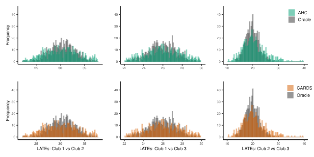
Figure C.1: Group-pair-LATEs: First and second step - club allocation and identification of invalid judges.

Note: Group-pair LATES after the first and second step of the procedure (detecting clubs with comparable propensity scores and eliminating invalid judges) for $\gamma=(0.5,0i_{3},0i_{2},0.4,0.6,0i_{2})$. Number of cases per judge: $Unif(3,5)\times 100$, $c=3$. Oracle: fully informed estimator, AHC: agglomerative hierarchical clustering, CARDS: AHC combined with a clustering algorithm in regression via data-driven segmentation.

D Application

D.1 Data

Table D.4: Descriptive Statistics

Variable	Overall	$D=1$	$D=0$	Diff	pval
Recidivism	0.292	0.3	0.219	0.08	4.4e-37
Female	0.183	0.173	0.276	-0.1	4.3e-53
Age at Sentence	33.04	33.02	33.2	-0.18	0.28
Race
White	0.59	0.585	0.638	-0.05	6.9e-13
Black	0.261	0.267	0.204	0.06	6.3e-24
Amerindian	0.073	0.074	0.065	0.01	0.021
Hispanic	0.05	0.047	0.074	-0.03	5.6e-12
Asian	0.026	0.027	0.018	0.01	5e-05
Unknown	0	0	0	0	0.73
Crime Type
Property Crime	0.332	0.324	0.412	-0.09	9.7e-32
Crime against a Person	0.299	0.306	0.235	0.07	8e-28
Drug Crime	0.238	0.242	0.2	0.04	7.5e-12
Sex Offenses	0.056	0.056	0.054	0	0.49
Weapons Offense	0.007	0.007	0.009	0	0.19
Other	0.068	0.065	0.091	-0.03	1.3e-09
Severity	3.44	3.46	3.25	0.21	6.1e-09

Note: ‘Overall’, ‘D = 1’ and ‘D = 0’, report the mean of the respective variable in the total sample, among the treated and the non-treated in the baseline sample of 2009-14 criminal cases. ‘Diff’ and ‘p-val’ provide the mean difference (across treatment states) and the p-value of a two-sample t-test.

Table D.5: Crimes considered in baseline sample

Crime Type	Crime Category	N
Theft	Property	3416
Theft of Firearm	Property	89
Theft Over 35K	Property	144
Possession of Shoplifting Gear	Property	85
Theft From Pers	Property	301
Theft of Motor Vehicle	Property	159
Motor Vehicle Use Without Consent	Property	1341
Receiving Stolen Property	Property	1330
Arson, 1st degree	Property	10
Arson, 2nd degree	Property	64
Arson, 3rd degree	Property	25
Burglary, 1st degree (Occupied Dwelling)	Property	483
Burglary, 2nd degree (Dwelling/Bank/Government Building/	Property	1330
Religious Est./ Historic Property/School Building)
Burglary, 2nd degree (Pharmacy/Tool)	Property	212
Burglary 3rd degree (Non Residential)	Property	1954
Possesion of Burglary Tools	Property	552
Criminal Damage	Property	617
Check Forgery (Over $35,000)	Property	8
Check Forgery (Over $2,500)	Property	276
Check Forgery ($251-$2,500)	Property	1144
Check Forgery ($250 or Less)	Property	81
Other Forgery	Property	306
Issuance of Dishonored Checks	Property	422
Financial Transaction Card Fraud	Property	989
Welfare/Unemployment Benefits/Food Stamp Fraud	Property	303
Identity Theft	Property	177
Possession or Sale of Counterfeit Check	Property	133
Mail Theft	Property	48
Other Property Crimes	Property	238
Criminal Vehicular Homicide or Injury, severity=5	Person	92
Criminal Vehicular Homicide or Injury, severity=3	Person	270
Assault, 2nd degree	Person	970
Assault, 3rd degree	Person	1637
Assault, 4th degree	Person	705
Assault, 5th degree	Person	253
Domestic Assault	Person	2280
Domestic Assault by Strangulation	Person	1147
Simple Robbery	Person	420
Aggravated Robbery, 1st degree	Person	88
Aggravated Robbery, 2nd degree	Person	102
Kidnapping (Safe Release/No Great Bodily Harm)	Person	17
Kidnapping (Unsafe Release/Great Bodily Harm/Victim Under 16)	Person	1
False Imprisonment	Person	65
Depriving Another of Cust. or Parental Rights	Person	37
Coercion	Person	13
Accidents	Person	9
Malicious Punishment of Child	Person	101
Threats of Violence (Terror/Evacuation)	Person	2900
Threats of Violence (Replica Firearm/Bomb Threat)	Person	87
Stalking, severity=4	Person	121
Stalking, severity=5	Person	160
Violation of Harassment Restraining Order	Person	2941
Tampering with a Witness	Person	24
Burglary 1st Degree (w/Weapon or Assault)	Person	8
Prostitution	Person	31
Other Person	Person	133
Controlled Substance Crime, 2nd degree	Drug	18
Controlled Substance Crime, 3rd degree	Drug	1454
Controlled Substance Crime, 4th degree	Drug	584
Controlled Substance Crime, 5th degree	Drug	9322
Possession of Substances with Intent to Manufacture Methamphetamine	Drug	46
Other Drug Offense	Drug	206
Drive-by Shooting (Unoccupied Motor Vehicle/Building)	Weapon	9
Discharge of Firearm	Weapon	139
Other Weapon Related Crimes	Weapon	204
Criminal Sexual Conduct, 2nd degree	Sex	240
Criminal Sexual Conduct, 3rd degree	Sex	373
Criminal Sexual Conduct, 4th degree	Sex	283
Criminal Sexual Conduct, 5th degree	Sex	4
Solicitation of Minors to Engage in Sexual Conduct	Sex	94
Failure to Register as Predator	Sex	1380
Possession of Child Pornography	Sex	334
Other Sex Crimes	Sex	12
Bribery	Other	13
Perjury	Other	35
Escape, severity=3	Other	240
Fleeing a Police Officer	Other	1660
Aiding Offender to Avoid Arrest	Other	124
Accomplice After the Fact	Other	54
Obstruction of Legal Procedure	Other	26
Lottery Fraud	Other	38
Felony Driving while Intoxicated	Other	530
Failure to Appear in Court	Other	65
Tax Offenses	Other	72
Other	Other	441

Note: Overview of the offenses considered in the application, the broader crime category to which each offense belongs, and the number of observations per offense in the baseline sample of 2009-14 criminal cases.

D.2 Figures

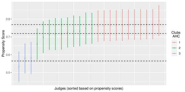
Figure D.2: First-stage clustering

Note: Minimum number of cases per judge: 300. On vertical axis: propensity scores with 95 percent confidence intervals. Dotted vertical lines denote cluster mean. Different colors denote different clubs.

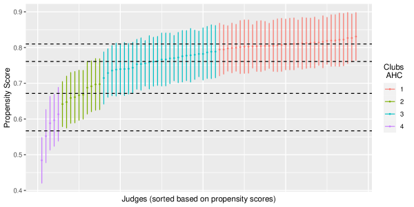
Figure D.3: First-stage clustering, min. 200 cases per judge

Note: Minimum number of cases per judge: 200. On vertical axis: propensity scores with 95 percent confidence intervals. Dotted vertical lines denote cluster mean. Different colors denote different clubs.

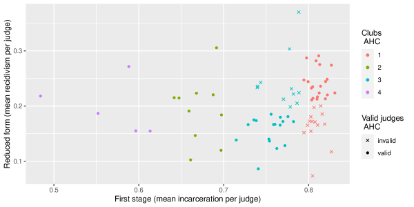
Figure D.4: Reduced-form clustering, min. 200 cases per judge

Note: Minimum number of cases per judge: 200. On vertical axis: mean outcomes per judge. Crosses denote judges selected as invalid, dots denote the selected validity set. Different colors denote different clubs.

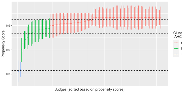
Figure D.5: First-stage clustering, subset analysis

Note: Subset analysis. On vertical axis: propensity scores with 95 percent confidence intervals. Dotted vertical lines denote cluster mean. Different colors denote different clubs.

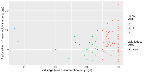
Figure D.6: Reduced-form clustering, subset analysis

Note: Subset analysis. On vertical axis: mean outcomes per judge. Crosses denote judges selected as invalid, dots denote the selected validity set. Different colors denote different clubs.

D.3 Additional results

Table D.6: First-stage clubs, 200

Club	Mean	Nr
1	0.81	34
2	0.67	10
3	0.76	28
4	0.57	5
5	0.14	1

Note: Clustering results when minimum case count per judge is 200.

Table D.7: Effect of Imprisonment on Recidivism, 200

	OLS	2SLS	1-2	1-3	1-4	2-3	2-4	3-4
Panel A: Post Club Clustering
D	0.061	0.051	0.030	0.37	-0.0077	-0.14	-0.035	-0.11
	(0.0096)	(0.025)	(0.10)	(0.18)	(0.077)	(0.17)	(0.18)	(0.100)
J			44	62	39	38	15	33
N	23958	23958	6901	9509	6140	5528	2159	4767
P		0.00	0.04	0.02	0.03	0.02	0.20	0.02
F		33.44	187.65	114.95	207.84	61.77	36.98	121.52

Panel B: Post Valid IV Selection
D			0.16	0.90	0.066	-0.41	-0.035	-0.18
			(0.11)	(0.23)	(0.080)	(0.21)	(0.18)	(0.11)
J			30	37	25	27	15	22
N			4793	5735	4032	3862	2159	3101
P			0.25	0.18	0.16	0.34	0.20	0.16
F			179.0	78.5	205.1	48.8	37.0	108.5
Note: Sample restricted so that minimum number of cases per judge is 200. Cluster-robust standard errors in parentheses. Significance level in testing procedure: 0.01. D: coefficient for LATE estimate when comparing judge clubs or groups as detailed in top line. Panel A: Results after club-clustering, without valid IV selection, Panel B: Results after valid IV selection. J: Number of judges, N: number of observations, P: p-value of Hansen-test from an over-identified specification.

D.4 Subset analysis

We tackle the problem of accounting for observable controls in an additional way by reducing the data to a subset with similar observables and perform the clustering of clubs inside this reduced dataset. We limit the data to male, white defendants of ages up to 100 with crimes against persons with a severity index equal to four. Moreover, we only look at judges with a minimum case count of 20, so that the calculation of propensity scores remains reliable.

Table D.8: First step clustering - Subset analysis

Club	Mean	Nr
1	0.97	80
2	0.81	21
3	0.35	2

In this case, the OLS estimate is statistically insignificant with a coefficient of 0.05, the 2SLS estimate is more than double the OLS estimate but it is still statistically indistinguishable from zero. When using algorithms 1 and 2 we find three clubs. The judge clubs have size 62, 39 and a small cluster with only two judges (see table D.8). When pairing these clubs, we find three unions of IVs (see table D.4). Pairing clubs two and one, we get a 2SLS estimate of almost 0.3, which is more precisely estimated. For the other two unions, the coefficient estimates are much lower and statistically insignificant. Hence, it seems that the initial 2SLS analysis was masking some heterogeneity in the Local Average Treatment Effects. We don’t proceed to the selection of invalid IVs at this step, because the Hansen-Sargan test is not rejected in the original 2SLS estimate. One main drawback of this analysis is that the first-stage F-statistics are worryingly low.

Table D.9: Effect of Imprisonment on Recidivism, Subset analysis

	OLS	2SLS	1-2	1-3	2-3
Panel A: Post Club Clustering
D	0.054	0.13	-0.027	0.070	0.095
	(0.028)	(0.071)	(0.32)	(0.13)	(0.17)
J			101	82	23
N	3280	3280	1605	1338	349
P		0.30	0.42	0.43	0.09
F		4.95	17.65	53.96	35.03

Panel B: Post Valid IV Selection
D			-0.027	0.070	0.095
			(0.32)	(0.13)	(0.17)
J			101	82	23
N			1605	1338	349
P			0.42	0.43	0.09
F			17.65	53.96	35.03
Note: Sample restricted to guarantee similar covariates. Cluster-robust standard errors in parentheses. Significance level in testing procedure: 0.1/log(N). D: coefficient for LATE estimate when comparing judge clubs or groups as detailed in top line. Panel A: Results after club-clustering, without valid IV selection, Panel B: Results after valid IV selection. J: Number of judges, N: number of observations, P: p-value of Hansen-test from an over-identified specification.

References

- Ana and Jain (2003) Ana, L. F. and A. K. Jain (2003). Robust data clustering. In 2003 IEEE Computer Society Conference on Computer Vision and Pattern Recognition, 2003. Proceedings., Volume 2, pp. II–II. IEEE.
- Andrews (1999) Andrews, D. W. (1999). Consistent Moment Selection Procedures for Generalized Method of Moments Estimation. Econometrica 67(3), 543–563.
- Angrist et al. (1996) Angrist, J., G. Imbens, and D. Rubin (1996). Identification of causal effects using instrumental variables. Journal of American Statistical Association 91(434), 444–472 (with discussion).
- Apfel and Liang (2021) Apfel, N. and X. Liang (2021). Agglomerative Hierarchical Clustering for Selecting Valid Instrumental Variables. arXiv preprint arXiv:2101.05774.
- Apfel and Windmeijer (2022) Apfel, N. and F. Windmeijer (2022). The falsification adaptive set in linear models with instrumental variables that violate the exogeneity or exclusion restriction. arXiv preprint arXiv:2212.04814.
- Bhuller et al. (2020) Bhuller, M., G. B. Dahl, K. V. Løken, and M. Mogstad (2020). Incarceration, recidivism, and employment. Journal of Political Economy 128(4), 1269–1324.
- Cortés et al. (2019) Cortés, T., N. Grau Veloso, and J. Rivera Cayupi (2019). Juvenile incarceration and adult recidivism.
- Fan and Li (2001) Fan, J. and R. Li (2001). Variable Selection via Nonconcave Penalized Likelihood and Its Oracle Properties. Journal of the American statistical Association 96(456), 1348–1360.
- Frandsen et al. (2023) Frandsen, B., L. Lefgren, and E. Leslie (2023). Judging Judge Fixed Effects. American Economic Review 113(1), 253–277.
- Frölich (2007) Frölich, M. (2007). Nonparametric iv estimation of local average treatment effects with covariates. Journal of Econometrics 139(5), 35–75.
- Green and Winik (2010) Green, D. P. and D. Winik (2010). Using random judge assignments to estimate the effects of incarceration and probation on recidivism among drug offenders. Criminology 48(2), 357–387.
- Guo et al. (2018) Guo, Z., H. Kang, T. T. Cai, and D. S. Small (2018). Confidence Intervals for Causal Effects with Invalid Instruments by Using Two-Stage Hard Thresholding with Voting. Journal of the Royal Statistical Society: Series B (Statistical Methodology) 80(4), 793–815.
- Heckman and Vytlacil (2001) Heckman, J. J. and E. Vytlacil (2001). Local instrumental variables. In C. Hsiao, K. Morimune, and J. Powell (Eds.), Nonlinear Statistical Inference: Essays in Honor of Takeshi Amemiya. Cambridge: Cambridge University Press.
- Heckman and Vytlacil (2005) Heckman, J. J. and E. Vytlacil (2005, May). Structural equations, treatment effects, and econometric policy evaluation 1. Econometrica 73(3), 669–738.
- Huber (2014) Huber, M. (2014). Sensitivity Checks for the Local Average Treatment Effect. Economics Letters 123(2), 220–223.