Surfaces away from horizons are not thermodynamic

Abstract

Since the 1970’s it has been known that black hole (and other) horizons are truly thermodynamic in nature. More generally, surfaces which are not horizons have also been conjectured to behave thermodynamically. Initially, for surfaces microscopically expanded from a horizon to so-called stretched horizons, and more recently, for more general ordinary surfaces in the emergent gravity program. To test these conjectures we ask whether such surfaces satisfy an analogue to the first law of thermodynamics (as do horizons). For static asymptotically-flat spacetimes we find that such a first law holds on horizons. We rigorously prove that this law remains an excellent approximation for stretched horizons, but perhaps counter-intuitively this result illustrates the insufficiency of the laws of black hole mechanics alone from implying truly thermodynamic behavior. For surfaces away from horizons in the emergent gravity program the first law fails (with the exception of fully spherically symmetric scenarios) thus undermining the key thermodynamic assumption of this program.

In 1973, Bardeen, Carter, and Hawking derived the laws of black hole mechanics which are in direct analogy with the laws of thermodynamics Bardeen1973 . Together with the discovery of Hawking radiation Hawking1975 , the truly thermodynamic behavior of black hole horizons became well established. Indeed such thermodynamic behavior is now well accepted for all spacetime horizons, including those due to accelerated observers unruh1976 ; jacobson1995 and cosmological horizons gibbons1977 .

Later, other surfaces were also attributed with thermodynamic properties. Firstly, stretched horizons were claimed to be thermodynamic, effectively acting as radiating black bodies Thorne1986 with a temperature $T=\kappa/(2\pi)$ determined by their local surface gravity $\kappa$ and an entropy (a ‘state variable’) associated with a statistical mechanical interpretation of black hole entropy Thorne1986 ; Thorne1985 . An explicit re-derivation of the laws of black hole mechanics has not been previously carried out for stretched horizons. More recently, a class of ordinary surfaces has been conjectured to behave thermodynamically, forming the key assumption in the emergent gravity program Verlinde2011 . This thermodynamic attribution was justified in part by using it in a heuristic derivation of the full Einstein field equations in static asymptotically-flat spacetime Verlinde2011 .

Here we ask whether canonical General Relativity is consistent with the assumption that such ordinary surfaces can be rigorously seen to behave thermodynamically. We attack this question by focusing on the analogue to the first law of thermodynamics. Originally this law was derived in an analysis that was specialized to the behavior of horizons Bardeen1973 . Here we remove this specialization to reveal the behavior of ordinary surfaces in an analysis of the first law.

Results

For a static asymptotically-flat spacetime with timelike Killing vector $K^{\mu}$ one may derive the total gravitating mass $M$ as an integral over a spacelike hypersurface $\Sigma$ that is truncated (or bounded) internally by an ordinary 2-surface $\partial\Sigma_{\text{in}}$ (see Fig. 1)

$$M=\frac{1}{4\pi}\int_{\Sigma}\!R_{\mu\nu}K^{\mu}\,\hat{T}^{\nu}\,\sqrt{|\gamma^{(\Sigma)}|}\;d^{3}x+\frac{1}{4\pi}\int_{\partial\Sigma_{\text{in}}}\!\!\!\!\kappa\;dA.$$ (1)

(See the Supplementary Information for a detailed derivation and definition of each term.) This expression is a straightforward extension of that used in 1973 by Bardeen et al. Bardeen1973 in their derivation of the first law of thermodynamics for black holes, though there the internal boundary was a horizon. Here $\kappa$ is a natural extension of the surface gravity for non-rotating spacetimes.

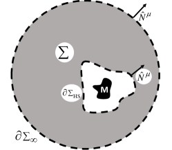
Figure 1: Schematic of the spacelike three-dimensional hypersurface of interest, $\Sigma$, with an inner boundary $\partial\Sigma_{\text{in}}$ and a boundary at infinity $\partial\Sigma_{\infty}$. Here $\hat{N}^{\mu}$ is the spacelike 4-vector normal to the boundaries of $\Sigma$ (note the direction convention on the inner boundary). We assume a general mass distribution within the inner boundary and no matter outside it.

Following the results for horizons Bardeen1973 , it is tempting to seek to interpret $\kappa/(2\pi)$ from Eq. (1) as the local temperature at any point along an arbitrary 2-surface $\partial\Sigma_{\text{in}}$. However, this would be unsatisfactory if true for arbitrary surfaces, since this local temperature would not be in thermal equilibrium with an actual physical screen held fixed at the same location; the temperature now coming from the Unruh effect unruh1976 and the local proper acceleration required to keep each portion of the screen stationary. Only for surfaces of constant Newtonian gravitational potential $\phi$, where the proper acceleration of a stationary observer and the local normal to the surface are parallel, is such thermal equilibrium possible (see Supplementary Information). Thus the temptation of such a thermodynamic interpretation should be restricted to the family of ordinary surfaces satisfying $\phi={\text{constant}}$.

Indeed, this restricted temptation appears to have been satisfied in the emergent gravity program, where for static asymptotically-flat spacetimes, ordinary surfaces of constant $\phi$ are dubbed holographic screens and are claimed to have a local temperature Verlinde2011 given by $T=\kappa/(2\pi)$ and even to possess a ‘state variable’ quantifying the number of ‘bits’ on the screen. These putative thermodynamic properties are then used in a heuristic derivation of the full Einstein field equations Verlinde2011 . If correct, such a claim would mean that the emergent gravity program would already subsume many decades of results associated with full General Relativity in this setting.

Here we test this thermodynamic assumption by asking whether perturbations of Eq. (1) reproduce the first law of thermodynamics. After all, thermodynamics is primarily a theory about how energy transforms under change, and this aspect of the theory is embodied in the first law. In the simplest case, where the hypersurface $\Sigma$ is empty of matter, this law should read

$$\delta M=\frac{1}{8\pi}\int_{\partial\Sigma_{\text{in}}}\!\!\!\!\kappa\;\delta(dA).$$ (2)

We start by following Bardeen et al.’s original analysis Bardeen1973 , generalizing it where necessary to deal with a boundary $\partial\Sigma_{\text{in}}$ which is an arbitrary ordinary surface instead of a horizon. Under diffeomorphic metric perturbations we find (see Supplementary Information)

$$\delta M\! = \!\frac{-1}{32\pi}\int_{\partial\Sigma_{\text{in}}}\!\!\!\bigl{[}4\delta\theta^{(l)}+(k_{3}+k_{6})\theta^{(l)}+(k_{3}-k_{6})\sigma_{+}^{(l)}$$ (3)

$$\leavevmode\nobreak\ \leavevmode\nobreak\ \leavevmode\nobreak\ \leavevmode\nobreak\ +(k_{4}+k_{5})\sigma_{\times}^{(l)}\bigr{]}\,{\cal N}dA+\frac{1}{8\pi}\int_{\partial\Sigma_{\text{in}}}\!\!\!\!\kappa\,\delta(dA).$$

Here $\theta^{(l)}$ and $\sigma_{j}^{(l)}$ ($j=+,\times$) are the expansion and shears of null normal congruences of geodesics, the change in the expansion under the diffeomorphism is given by

$$\delta\theta^{(l)}=-\frac{k_{2}}{2}\theta^{(l)}+\frac{1}{2}(k_{3}+k_{6})_{;\rho}\hat{N}^{\rho},$$ (4)

and the $k_{j}$ are functions corresponding to independent components of the metric perturbation. As the expansion and shears vanish identically on the horizon hawking1973 , we see that Eq. (3) trivially reduces to the first law, Eq. (2), thus reproducing the famous 1973 result Bardeen1973 . Similarly, it follows straightforwardly that for surfaces sufficiently close to the horizon (so-called stretched horizons), the corrections to the first law will be negligible.

So far we have assumed that the inner boundaries before and after the diffeomorphic perturbation are arbitrary. But could the perturbed boundary be chosen in a specific manner so as to cause the unwanted terms in Eq. (3) to vanish? As already noted, holographic screens correspond to surfaces of constant Newtonian potential $\phi={\text{constant}}$. Thus, the perturbed screen relies on a specification of the constant $\delta\phi$. It is easy to show that $\delta\phi=\frac{1}{2}k_{1}$ (see Supplementary Information), where $k_{1}$ is a metric perturbation of which the unwanted terms in Eq. (3) are wholly independent. Thus, the ordinary surfaces used within the emergent gravity program cannot generally satisfy the first law, Eq. (2).

One caveat to this claim comes when we consider a fully spherically symmetric scenario; where both the initial spacetime and screen are spherically symmetric, so the initial shears $\sigma_{j}^{(l)}$ vanish, and also the final spacetime and screen are spherically symmetric, placing further constraints on the $k_{j}$. In this case, Birkhoff’s theorem Birkhoff1923 for spherically symmetric metrics imposes extra constraints between the metric components so that a perturbed screen may always be chosen so as to satisfy the form of the first law Chen11 . However, as noted above, this form will not be preserved under arbitrary metric perturbations.

Discussion

The implications of our results are now described for (i) stretched horizons, and (ii) ordinary surfaces.

(i) Stretched horizons have long been considered to act as black bodies Thorne1986 , effectively radiating with a temperature $\kappa/(2\pi)$. Thus, our demonstration that they also satisfy the first law to an excellent approximation hardly seems surprising. Nevertheless, we do not believe that our result here should be interpreted as implying that the surfaces corresponding to stretched horizons themselves should be imbued with actual thermodynamic properties.

In particular, we may consider an alternative spacetime, identical from the stretched horizon outward, but instead of a horizon, we consider an infinitesimal shell of matter just outside what would correspond to its Schwarzschild radius were the shell to collapse further, yet still within the ‘stretched horizon’. In this latter spacetime, there is no horizon and hence no Hawking radiation. Notwithstanding this, our work proves that the ‘stretched horizon’ still closely satisfies the first law.

We conclude from this that the laws of black hole mechanics are not sufficient in themselves to guarantee whether any particular surface is truly thermodynamic in nature. For stretched horizons, we interpret this reasoning to imply that their full thermodynamic behavior is only inherited from the presence of an underlying horizon, but is not intrinsic to stretched horizons themselves. This conclusion appears to mimic the initial reluctance of general relativistsBardeen1973 from accepting black hole horizons as truly thermodynamic despite the deep analogy to thermodynamics uncovered in the laws of black hole mechanics. By contrast, these laws should still be considered a necessary condition.

(ii) Our analysis further rigorously shows that the family of ordinary surfaces called holographic screens will generally not obey a first law of thermodynamics, in contrast to the long-standing result for horizons Bardeen1973 . (Other families would not even be in thermal equilibrium with a physical surface at the same location.) Recall that the first law is more general than thermodynamics: the ‘temperature’ is merely an integrating factor relating changes in energy to changes in some state variable (entropy in the case of thermodynamics). Failure of the first law means that the putative state variable is not a variable of state at all. Therefore, even in static asymptotically-flat spacetimes, where the emergent gravity program claims to derive the full Einstein field equations, our results show that the key assumption of this program is actually inconsistent with General Relativity.

Methods

In order to attempt to derive a first law for ordinary surfaces we closely follow in the footsteps of Bardeen, Carter and Hawking’s 1973 classic paper Bardeen1973 . The first step is to obtain an integral equation for the net energy in a static system, Eq. (1), where instead of an inner boundary located at a black hole horizon, this boundary is an ordinary surface. Next, we consider small ‘changes’ in the net energy corresponding to shifting to a parametrically nearly solution to the Einstein field equations. This ‘differential’ version is determined by studying the behavior of the net energy under spacetime diffeomorphisms of the initial metric Bardeen1973 . As in Bardeen et al., “gauge” freedom in the choice of coordinates is used to ensure that the hypersurfaces before and after the diffeomorphism are covered by identical sets of coordinates.

Our analysis is limited to static asymptotically-flat solutions, with zero shift vector, $\beta^{\mu}=0$. For simplicity, we assume that the spacetime of interest is non-rotating, and that there is no matter exterior to the holographic screen ($T^{\mu\nu}=0$). We work throughout in natural units where $G=c=\hbar=k_{B}=1$. Full and extensive details of the analysis are provided in the Supplementary Information.

Appendix

.1 List of key symbols

We set $G=c=\hbar=k_{B}=1$ throughout. A list of key symbols used in the Appendix:

$M$

mass

${\cal N}$

lapse function ($=1/\hat{T}^{t}$)

$\beta^{\mu}$

shift vector ($=0$ throughout)

$g_{\mu\nu}$

metric

$T^{\mu\nu}$

energy-momentum tensor ($=0$ from Eq.(24))

$R_{\mu\nu}$

curvature tensor

$R$

Ricci scalar

$\Sigma$

3-dimensional hypersurface in this paper

$\Sigma_{\text{EG}}$

3-dimensional hypersurface in Ref. Verlinde2011,

$\partial\Sigma$

boundary of $\Sigma$

$\partial\Sigma_{\infty}$

outer boundary of $\Sigma$

$\partial\Sigma_{\text{in}}$

inner boundary of $\Sigma$ (ordinary surface)

$\partial\Sigma_{\text{BH}}$

inner boundary of $\Sigma$ (black hole horizon)

$\partial\Sigma_{\text{HS}}$

inner boundary of $\Sigma$ (holographic screen)

$\gamma^{(\Sigma)}$

induced metric on $\Sigma$

$\gamma^{(\partial\Sigma)}$

induced metric on $\partial\Sigma$

$dA$

area element ($=\sqrt{\gamma^{(\partial\Sigma)}}\,dy^{2}$)

$\hat{T}^{\mu}$

timelike unit normal vector of $\Sigma$

$\hat{N}^{\mu}$

spacelike unit normal vector of $\partial\Sigma$

$\kappa$

generalized surface gravity, Eq. (11)

$K^{\mu}$

Killing vector of the static spacetime ($=\partial_{t}$)

$h_{\mu\nu}$

diffeomorphic variation of the metric ($=\delta g_{\mu\nu}$)

$\theta^{(l)}$

expansion of the outgoing null normal vector $l^{\mu}$

$\sigma_{+}^{(l)},\,\sigma_{\times}^{(l)}$

shears of the outgoing null normal vector $l^{\mu}$

$\sigma_{P}^{(l)}$

‘principle shear’ of the outgoing null normal vector $l^{\mu}$

.2 Integral expression for net energy

Consider a static spacetime with a Killing vector $K^{\mu}=\partial_{t}=(1,0,0,0)$, with $K^{\mu}K_{\mu}=-1$ at spatial infinity. The Killing equation implies that

$$K_{\mu;\nu}=K_{[\mu;\nu]}\equiv\frac{1}{2}(K_{\mu;\nu}-K_{\nu;\mu})\;.$$ (5)

Now recall that permuting the order of a pair of covariant derivatives acting on a 4-vector $A^{\mu}$ may be expressed in terms of the Riemann curvature tensor as carroll2004

$${A^{\mu}}_{;\alpha\beta}-{A^{\mu}}_{;\beta\alpha}=-{R^{\mu}}_{\nu\alpha\beta}A^{\nu}\;.$$

Contracting the indices $\mu$ and $\alpha$ reduces this to an expression in terms of the Ricci tensor

$${A^{\mu}}_{;\mu\beta}-{A^{\mu}}_{;\beta\mu}=-R_{\nu\beta}A^{\nu}\;.$$ (6)

Since the Killing vector is anti-symmetric we must have ${K^{\mu}}_{;\mu}=0$ and we immediately find that

$${K^{\mu}}_{;\beta\mu}=R_{\nu\beta}K^{\nu}.$$ (7)

Integrating this over a spacelike hypersurface $\Sigma$, yields

$$\int_{\Sigma}{K^{\mu}}_{;\beta\mu}\,\hat{T}^{\beta}\,\sqrt{|\gamma^{(\Sigma)}|}\,d^{3}x=\int_{\Sigma}R_{\nu\beta}K^{\nu}\,\hat{T}^{\beta}\,\sqrt{|\gamma^{(\Sigma)}|}\,d^{3}x$$ (8)

here $\hat{T}^{\mu}$ is the timelike unit 4-vector normal to $\Sigma$, so $\hat{T}^{\mu}\hat{T}_{\mu}=-1$.

The hypersurface is assumed to have an outer boundary at spatial infinity $\partial\Sigma_{\infty}$, and an inner boundary $\Sigma_{\text{in}}$ (see Fig. 1). In the original work of Bardeen et al. Bardeen1973 , this inner boundary corresponded to the black hole’s horizon $\partial\Sigma_{\text{BH}}$. Here we generalize this by taking it to be an arbitrary closed 2-surface $\partial\Sigma_{\text{in}}$. The boundary of the hypersurface is assumed to be oriented, with unit normal $\hat{N}^{\mu}$ (see Fig. 1), so $\hat{N}_{\mu}\hat{N}^{\mu}=1$ and $\hat{N}^{\mu}\hat{T}_{\mu}=0$.

Recalling Stokes’s theorem for an anti-symmetric tensor $F^{\mu\nu}$ carroll2004

$$\int_{\Sigma}\hat{T}_{\mu}{F^{\mu\nu}}_{;\nu}\sqrt{|\gamma^{(\Sigma)}|}dx^{n-1}=\int_{\partial\Sigma}\hat{T}_{\mu}F^{\mu\nu}\hat{N}_{\nu}\sqrt{|\gamma^{(\partial\Sigma)}|}dy^{n-2},$$ (9)

and applying it to the left-hand-side of Eq. (8) we find

$$\int_{\partial\Sigma_{\infty}}{K^{\mu}}_{;\beta}\,\hat{T}^{\beta}\hat{N}_{\mu}\sqrt{|\gamma^{(\partial\Sigma_{\infty})}|}\;d^{2}y-\int_{\partial\Sigma_{\text{in}}}{K^{\mu}}_{;\beta}\,\hat{T}^{\beta}\hat{N}_{\mu}\,\sqrt{|\gamma^{(\partial\Sigma_{\text{HS}})}|}\;d^{2}y=\int_{\Sigma}R_{\nu\beta}K^{\nu}\,\hat{T}^{\beta}\,\sqrt{|\gamma^{(\Sigma)}|}\,d^{3}x.$$ (10)

At this stage, we wish to generalize the concept of surface gravity as a quantity defined anywhere. Assuming that the surface $\partial\Sigma$ is non-rotating (corresponding to zero angular velocity of the spacetime itself) , we may interpret the integrand of the integral on the boundary in Eq. (10) to be the surface gravity, so

$$\boxed{\kappa\equiv{K^{\mu}}_{;\nu}\hat{T}^{\nu}\hat{N}_{\mu}.}$$ (11)

It is worth noting that ${\kappa}/({2\pi})$ is precisely the formula Verlinde gives (his Eq. (5.3) of Ref. [Verlinde2011, ]) for what he calls the local temperature of the holographic screen (ordinary surfaces of constant Newtonian potential $\phi$) as measured with respect to a reference point at spatial infinity.

This definition of surface gravity allows us to naturally extend the original 1973 analysis away from black hole horizons. In particular, the left-hand-side of Eq. (10) reduces to

$$\int_{\partial\Sigma_{\infty}}\kappa\,\sqrt{|\gamma^{(\partial\Sigma_{\infty})}|}\;d^{2}y-\int_{\partial\Sigma_{\text{in}}}\kappa\,\sqrt{|\gamma^{(\partial\Sigma_{\text{HS}})}|}\;d^{2}y.$$ (12)

The integral over $\partial\Sigma_{\infty}$ reduces to the Komar expression for the total gravitating mass within the system, $M$, carroll2004 leading to

$$\boxed{M=\frac{1}{4\pi}\int_{\Sigma}R_{\mu\nu}K^{\mu}\,\hat{T}^{\nu}\,\sqrt{|\gamma^{(\Sigma)}|}\;d^{3}x+\frac{1}{4\pi}\int_{\partial\Sigma_{\text{in}}}\!\!\kappa\;dA\;,}$$

(13)

Were we to consider spherically symmetric case, Eq. (13) would reduce to

$$M=\frac{1}{4\pi}\int_{\Sigma}R_{\mu\nu}K^{\mu}\,\hat{T}^{\nu}\,\sqrt{|\gamma^{(\Sigma)}|}\,d^{3}x+\frac{\kappa}{4\pi}A.$$ (14)

(This is exactly the first law given by Bardeen et al. Bardeen1973 taking angular velocity of $\partial\Sigma$ to vanish).

Just to emphasize what this represents, here the hypersurface, $\Sigma$, extends from an arbitrary inner boundary, $\partial\Sigma_{\text{in}}$, out to spatial infinity. Thus, the generalized surface gravity, $\kappa$, and the area, $A$, are those associated with the inner boundary itself (rather than any horizon).

Eq. (13) has exactly the same form as the conventional formula for the total mass of the system Bardeen1973 but extended to an arbitrary 2-dimensional surface (instead of a horizon). Finally, note that the matter inside the inner boundary need not be associated with a black hole, it may be ordinary matter, with no horizon present at all. Thus, were inner boundaries found to have thermodynamic properties (i.e., a well-defined entropy and temperature), it would not be because such properties were inherited from a real horizon behind the screen.

.3 Differential “first law”

The above straightforward generalization, especially in the spherically symmetric case, for net energy on a hypersurface might appear to suggest that a temperature and entropy can actually be defined for any surface by

$$T=\frac{\kappa}{2\pi},\qquad\qquad S=\frac{A}{4}.$$ (15)

However, such quantities need to behave thermodynamically. In particular, for our static system, the net energy $E$, should admit changes which behave as

$$\delta E=T\delta S,$$ (16)

(ignoring work terms) so that the temperature would be acting as an integrating factor relating changes in the (state function) entropy to changes in the energy. In other words, we must show that such changes lead to the expected form of the first-law of thermodynamics. Again here we follow in the footsteps of the original analysis and consider changes corresponding to parametric differences between diffeomorphicly nearby solutions. In particular, we will consider two nearby configurations corresponding to the metrics

$$g_{\mu\nu},\qquad\qquad g^{\prime}_{\mu\nu}=g_{\mu\nu}+h_{\mu\nu},$$ (17)

where $h_{\mu\nu}\equiv\delta g_{\mu\nu}=-g_{\mu\sigma}g_{\nu\tau}\delta g^{\sigma\tau}$, i.e., $\delta g^{\sigma\tau}=-h^{\sigma\tau}$.

As with the original analysis and without loss of generality, we may assume that for the two diffeomorphicly related configurations, the hypersurfaces $\Sigma$ and $\Sigma^{\prime}$ are described by identical sets of coordinates; this is always possible due to “gauge” freedom in the choice of coordinate systems Bardeen1973 . Henceforth we label both by $\Sigma$. Similarly, for their boundaries $\partial\Sigma$. Further, as in Bardeen1973 we likewise assume that both configurations have the same Killing vector, so

$$\delta K^{\mu}=0,\qquad\qquad\delta K_{\mu}=h_{\mu\nu}K^{\nu}.$$ (18)

Finally, it will be sufficient for our purposes to consider only the case where there is no matter on $\Sigma$ itself, so $T^{\mu\nu}=0$ there. Geometrically, this corresponds to all the matter lying behind or within the inner boundary $\partial\Sigma_{\text{in}}$ (see Fig. 1).

In order to consider diffeomorphisms which need not respect spherical symmetry, we return to Eq. (13). Using the Einstein field equations we start by rewriting this integral formula as

$$M=\int_{\Sigma}(2\,T_{\mu\nu}+\frac{1}{8\pi}R\,g_{\mu\nu})K^{\mu}\,\hat{T}^{\nu}\,\sqrt{|\gamma^{(\Sigma)}|}\,d^{3}x+\frac{1}{4\pi}\int_{\partial\Sigma_{\text{in}}}\kappa\;dA\;,$$ (19)

Recall $K^{\mu}=\partial_{t}$ and $\hat{T}^{\mu}$ is normal to $\Sigma$, so $K^{\mu}={\cal N}\hat{T}^{\mu}+\beta^{\mu}$ where $\beta^{\mu}$ is the shift vector and ${\cal N}=1/\hat{T}^{t}$ is the lapse function gourgoulhon2012 . Assuming a zero shift vector $\beta^{\mu}=0$, then $\hat{T}^{\mu}=\hat{T}^{t}K^{\mu}$ and $\hat{T}_{\mu}=\hat{T}^{t}K_{\mu}$. Since ${\cal N}\sqrt{|\gamma^{(\Sigma)}|}=\sqrt{-g}$ on the hypersurface gourgoulhon2012 , the variation of the Ricci scalar term may be computed as

$$\frac{1}{8\pi}\int_{\Sigma}\delta(R\sqrt{|\gamma^{(\Sigma)}|}\,K^{\beta}\,\hat{T}_{\beta})\,d^{3}x$$ (20)

$$= \frac{1}{8\pi}\int_{\Sigma}\delta(R\,{\cal N}\sqrt{|\gamma^{(\Sigma)}|}\,\hat{T}^{\beta}\,\hat{T}_{\beta})\,d^{3}x$$

$$= \frac{1}{8\pi}\int_{\Sigma}\delta(R\,\sqrt{-g})\,\hat{T}^{\beta}\,\hat{T}_{\beta}\,d^{3}x$$

$$= -\frac{1}{8\pi}\int_{\Sigma}\Bigl{(}(R_{\mu\nu}-\frac{1}{2}g_{\mu\nu}R)h^{\mu\nu}-(g^{\mu\nu}\delta{\Gamma^{\alpha}}_{\mu\nu}-g^{\mu\alpha}\delta{\Gamma^{\lambda}}_{\lambda\mu})_{;\alpha}\Bigl{)}\,K^{\beta}\,\hat{T}_{\beta}\,\sqrt{|\gamma^{(\Sigma)}|}\,d^{3}x\;.$$

where in the last step we have used the well-known result that bertschinger2002

$$\delta(R\sqrt{-g})=-\Bigl{(}(R_{\mu\nu}-\frac{1}{2}g_{\mu\nu}R)h^{\mu\nu}-(g^{\mu\nu}\delta{\Gamma^{\alpha}}_{\mu\nu}-g^{\mu\alpha}\delta{\Gamma^{\lambda}}_{\lambda\mu})_{;\alpha}\Bigr{)}\sqrt{-g}.$$ (21)

Lemma 1: $-(g^{\mu\nu}\delta{\Gamma^{\alpha}}_{\mu\nu}-g^{\mu\alpha}\delta{\Gamma^{\lambda}}_{\lambda\mu})_{;\alpha}=2\,{{h^{\mu}}_{[\mu;\nu]}}^{;\nu}$, a result quoted in Ref. Bardeen1973 , there without proof.

Proof:

Since palatini1919

$$\delta\Gamma_{\mu\nu}^{\alpha}=\frac{1}{2}g^{\alpha\rho}(h_{\mu\rho;\nu}+h_{\nu\rho;\mu}-h_{\mu\nu;\rho})\;,$$ (22)

we have

$$-(g^{\mu\nu}\delta{\Gamma^{\alpha}}_{\mu\nu}-g^{\mu\alpha}\delta{\Gamma^{\lambda}}_{\lambda\mu})_{;\alpha} = \Bigl{(}g^{\mu\alpha}\frac{1}{2}g^{\lambda\rho}(h_{\mu\rho;\lambda}+h_{\lambda\rho;\mu}-h_{\mu\lambda;\rho})-g^{\mu\nu}\frac{1}{2}g^{\alpha\rho}(h_{\mu\rho;\nu}+h_{\nu\rho;\mu}-h_{\mu\nu;\rho})\Bigr{)}_{;\alpha}$$ (23)

$$= \frac{1}{2}\Bigl{(}g^{\mu\alpha}{h^{\rho}}_{\rho;\mu}-g^{\mu\nu}({h^{\alpha}}_{\mu;\nu}+{h^{\alpha}}_{\nu;\mu}-{h_{\mu\nu}}^{;\alpha})\Bigr{)}_{;\alpha}$$

$$= \frac{1}{2}\Bigl{(}{h_{\rho}}^{\rho;\alpha}-({h^{\alpha\nu}}_{;\nu}+{h^{\alpha\mu}}_{;\mu}-{h_{\mu}}^{\mu;\alpha})\Bigr{)}_{;\alpha}$$

$$= \frac{1}{2}(2\,{h_{\rho}}^{\rho;\alpha}-2\,{h^{\alpha\mu}}_{;\mu})_{;\alpha}$$

$$= 2\,{{h^{\mu}}_{[\mu;\nu]}}^{;\nu}.$$

This completes the proof of Lemma 1. ∎

Using Lemma 1, the variation of the Ricci scalar term becomes

$$-\frac{1}{8\pi}\int_{\Sigma}\Bigl{(}(R_{\mu\nu}-\frac{1}{2}g_{\mu\nu}R)h^{\mu\nu}+2{{h^{\mu}}_{[\mu;\nu]}}^{;\nu}\Bigl{)}\,K^{\beta}\,\hat{T}_{\beta}\,\sqrt{|\gamma^{(\Sigma)}|}\,d^{3}x=-\frac{1}{4\pi}\int_{\Sigma}{{h^{\mu}}_{[\mu;\nu]}}^{;\nu}K^{\beta}\,\hat{T}_{\beta}\,\sqrt{|\gamma^{(\Sigma)}|}\,d^{3}x$$ (24)

since the first term is zero if we assume $T^{\mu\nu}=0$ on $\Sigma$ outside the holographic screen.

Lemma 2: ${{h^{\mu}}_{[\mu;\nu]}}^{;\nu}K^{\beta}=(K^{\beta}{h_{\mu}}^{[\mu;\nu]}-K^{\nu}{h_{\mu}}^{[\mu;\beta]})_{;\nu}$, a result quoted in Ref. Bardeen1973 , there without proof.

Proof: Expanding out the right-hand-side (rhs) of the claim in Lemma 2, we get

$$\text{rhs}={{h_{\mu}}^{[\mu;\nu]}}_{;\nu}K^{\beta}+{h_{\mu}}^{[\mu;\nu]}{K^{\beta}}_{;\nu}-{{h_{\mu}}^{[\mu;\beta]}}_{;\nu}K^{\nu}\;\;,$$ (25)

since ${{h_{\mu}}^{[\mu;\nu]}}_{;\nu}K^{\beta}={{h^{\mu}}_{[\mu;\nu]}}^{;\nu}K^{\beta}$, Eq. (25) reduces to

$${{h^{\mu}}_{[\mu;\nu]}}^{;\nu}K^{\beta}+{h_{\mu}}^{[\mu;\nu]}{K^{\beta}}_{;\nu}-{{h_{\mu}}^{[\mu;\beta]}}_{;\nu}K^{\nu}={{h^{\mu}}_{[\mu;\nu]}}^{;\nu}K^{\beta}-\pounds_{K}({h_{\mu}}^{[\mu;\beta]})={{h^{\mu}}_{[\mu;\nu]}}^{;\nu}K^{\beta}=\text{lhs}\;.$$ (26)

The Lie derivative along $K^{\mu}$ vanishes since the pair of diffeomorphicly related metrics are assumed static poisson2004 . This completes the proof of Lemma 2. ∎

Applying Lemma 2 to Eq. (24), the variation of the term involving the Ricci scalar reduces to

$$-\frac{1}{4\pi}\int_{\Sigma}(K^{\beta}{h_{\mu}}^{[\mu;\nu]}-K^{\nu}{h_{\mu}}^{[\mu;\beta]})_{;\nu}\,\hat{T}_{\beta}\,\sqrt{|\gamma^{(\Sigma)}|}\,d^{3}x.$$ (27)

Thus, the variation in the total mass may be written

$$\delta M=-\frac{1}{4\pi}\int_{\Sigma}(K^{\beta}{h_{\mu}}^{[\mu;\nu]}-K^{\nu}{h_{\mu}}^{[\mu;\beta]})_{;\nu}\,\hat{T}_{\beta}\,\sqrt{|\gamma^{(\Sigma)}|}\,d^{3}x+\frac{1}{4\pi}\int_{\partial\Sigma_{\text{in}}}\delta\kappa\;dA+\frac{1}{4\pi}\int_{\partial\Sigma_{\text{in}}}\kappa\;\delta(dA).$$ (28)

Since the term inside the bracket is an anti-symmetric tensor, we may use Stokes’s theorem, Eq. (9), to obtain

$$\delta M= -\frac{1}{4\pi}\int_{\partial\Sigma_{\infty}}(K^{\beta}{h_{\mu}}^{[\mu;\nu]}-K^{\nu}{h_{\mu}}^{[\mu;\beta]})\hat{N}_{\nu}\,\hat{T}_{\beta}\,\sqrt{|\gamma^{({\partial\Sigma_{\infty}})}|}\,d^{2}y$$ (29)

$$+\frac{1}{4\pi}\int_{\partial\Sigma_{\text{in}}}(K^{\beta}{h_{\mu}}^{[\mu;\nu]}-K^{\nu}{h_{\mu}}^{[\mu;\beta]})\hat{N}_{\nu}\,\hat{T}_{\beta}\,\sqrt{|\gamma^{({\partial\Sigma_{\text{in}}})}|}\,d^{2}y+\frac{1}{4\pi}\int_{\partial\Sigma_{\text{in}}}\delta\kappa\;dA+\frac{1}{4\pi}\int_{\partial\Sigma_{\text{in}}}\kappa\;\delta(dA),$$

where the boundary has be split into the inner boundary $\partial\Sigma_{\text{in}}$ and the boundary at infinity $\partial\Sigma_{\infty}$. The contribution for the term at infinity may be evaluated using the notation of tensorial volume elements Wald1984 as

$$-\frac{1}{4\pi}\int_{\partial\Sigma_{\infty}}(K^{\beta}{h_{\mu}}^{[\mu;\nu]}-K^{\nu}{h_{\mu}}^{[\mu;\beta]})\hat{N}_{\nu}\,\hat{T}_{\beta}\,\sqrt{|\gamma^{(\partial\Sigma_{\infty})}|}\,d^{2}y = -\frac{1}{4\pi}\int_{\partial\Sigma_{\infty}}K^{\beta}{h_{\mu}}^{[\mu;\nu]}(\hat{T}_{\beta}\,\hat{N}_{\nu}\,-\hat{T}_{\nu}\,\hat{N}_{\beta})\sqrt{|\gamma^{(\partial\Sigma_{\infty})}|}\,d^{2}y$$ (30)

$$= -\frac{1}{4\pi}\int_{\partial\Sigma_{\infty}}K^{\beta}{h_{\mu}}^{[\mu;\nu]}\,\varepsilon_{\beta\nu}\,\varepsilon_{\alpha\mu}$$

$$= \frac{1}{8\pi}\int_{\partial\Sigma_{\infty}}({h_{\mu}}^{\mu;\nu}-{h_{\mu}}^{\nu;\mu})K^{\beta}\,\varepsilon_{\beta\nu\alpha\mu}$$

$$= -\delta M\;,$$

where the orientation of $\varepsilon_{\beta\nu\alpha\mu}$ is chosen so that $\varepsilon_{\beta\nu\alpha\mu}=-6\,\varepsilon_{[\beta\nu}\varepsilon_{\alpha\mu]}$ and $\varepsilon_{\alpha\mu}$ is the volume element of the boundary at infinity, and we have applied the result $\frac{1}{8\pi}\int_{\partial\Sigma_{\infty}}({h_{\mu}}^{\mu;\nu}-{h_{\mu}}^{\nu;\mu})K^{\beta}\,\varepsilon_{\beta\nu\alpha\mu}=-\delta M$ in the final step Wald1984 .

Eq. (30) allows us to transform Eq. (29) into

$$\delta M=-\delta M+\frac{1}{4\pi}\int_{\partial\Sigma_{\text{in}}}(K^{\beta}{h_{\mu}}^{[\mu;\nu]}-K^{\nu}{h_{\mu}}^{[\mu;\beta]})\hat{N}_{\nu}\,\hat{T}_{\beta}\,\sqrt{|\gamma^{({\partial\Sigma_{\text{in}}})}|}\,d^{2}y+\frac{1}{4\pi}\int_{\partial\Sigma_{\text{in}}}\delta\kappa\;dA+\frac{1}{4\pi}\int_{\partial\Sigma_{\text{in}}}\kappa\;\delta(dA).$$ (31)

Or equivalently,

$$\delta M=\frac{1}{8\pi}\int_{\partial\Sigma_{\text{in}}}\frac{1}{2}({h_{\mu}}^{\mu;\nu}-{h_{\mu}}^{\nu;\mu})\hat{N}_{\nu}\,\hat{T}_{\beta}K^{\beta}\,dA+\frac{1}{8\pi}\int_{\partial\Sigma_{\text{in}}}\delta\kappa\;dA+\frac{1}{8\pi}\int_{\partial\Sigma_{\text{in}}}\kappa\;\delta(dA)\;,$$ (32)

where we have used $K^{\nu}\hat{N}_{\nu}={\cal N}\hat{T}^{\nu}\hat{N}_{\nu}=0$, which follows since $\hat{T}^{\mu}$ is normal to $\Sigma$ and $\hat{N}^{\mu}$ lies in $\Sigma$.

For the first law to be true, we would require that the first two boundary integrals of Eq. (32) exactly cancel. In order to further simplify these terms we start by considering the diffeomorphic changes in more detail.

.4 Diffeomorphic conditions

As already discussed, we assume

$$\delta K^{\mu}=0,\qquad\qquad\delta K_{\mu}=h_{\mu\nu}K^{\nu}.$$ (33)

Recall that by “gauge” freedom the sets of coordinates of $\Sigma$ and $\partial\Sigma$ are unchanged by the diffeomorphism, so without loss of generality we may take Bardeen1973

$$\delta(dx^{\mu})=0\;,\forall dx^{\mu}\;\text{in}\;\Sigma.$$ (34)

Because $K_{\mu}dx^{\mu}={\cal N}\hat{T}_{\mu}dx^{\mu}=0$ for all $dx^{\mu}$ in $\Sigma$, we have $\delta K_{\mu}\parallel K_{\mu}$, so

$$\delta K_{\mu}=k_{0}K_{\mu}.$$ (35)

Comparing Eq. (35) with Eq. (33), one finds

$$h_{\mu\nu}K^{\nu}=k_{0}K_{\mu}$$ (36)

everywhere. Then contracting $\hat{T}^{\mu}$ on both sides of this equation yields

$$k_{0}=-h_{\mu\nu}\hat{T}^{\mu}\hat{T}^{\nu}.$$ (37)

(In other words, $k_{0}=-h_{\hat{T}\hat{T}}$ in the tetrad basis.)

Similarly, since $\hat{T}_{\mu}dx^{\mu}=0$ for all $dx^{\mu}$ in $\Sigma$, we have $\delta\hat{T}_{\mu}\parallel\hat{T}_{\mu}$, so

$$\delta\hat{T}_{\mu}=\frac{k_{1}}{2}\hat{T}_{\mu}$$ (38)

(the factor of $\frac{1}{2}$ is for later convenience). To get an expression for $k_{1}$, we calculate the variation of $g^{\mu\nu}\hat{T}_{\mu}\hat{T}_{\nu}=-1$.

$$(\delta g^{\mu\nu})\hat{T}_{\mu}\hat{T}_{\nu}+2g^{\mu\nu}\hat{T}_{\mu}(\delta\hat{T}_{\nu}) = 0$$

$$\Rightarrow\;\;\;\;(-h^{\mu\nu})\hat{T}_{\mu}\hat{T}_{\nu}+2g^{\mu\nu}\hat{T}_{\mu}(\frac{k_{1}}{2}\hat{T}_{\nu}) = 0,$$ (39)

hence

$$k_{1}=-h_{\mu\nu}\hat{T}^{\mu}\hat{T}^{\nu}=k_{0}.$$ (40)

For $\hat{T}^{\mu}$, we find

$$\delta\hat{T}^{\mu} = \delta(g^{\mu\nu}\hat{T}_{\nu})$$ (41)

$$= -h^{\mu\nu}\hat{T}_{\nu}+\frac{1}{2}k_{1}\hat{T}^{\mu}$$

$$= -g^{\mu\lambda}h_{\lambda\nu}\hat{T}^{\nu}+\frac{1}{2}k_{1}\hat{T}^{\mu}$$

$$= -g^{\mu\lambda}h_{\lambda\nu}K^{\nu}\hat{T}^{t}+\frac{1}{2}k_{1}\hat{T}^{\mu}$$

$$= -g^{\mu\lambda}k_{1}K_{\lambda}\hat{T}^{t}+\frac{1}{2}k_{1}T^{\mu}$$

$$= -k_{1}\hat{T}^{\mu}+\frac{1}{2}k_{1}\hat{T}^{\mu}$$

$$= -\frac{1}{2}k_{1}\hat{T}^{\mu},$$

where we have used Eq. (36) in the fourth line.

Again since, $dx^{\mu}\hat{N}_{\mu}=0$ for all $dx^{\mu}$ in $\partial\Sigma$, combined with $\hat{T}^{\mu}\hat{N}_{\mu}=0$, we find $\delta\hat{N}_{\mu}\parallel\hat{N}_{\mu}$, and so we write

$$\delta\hat{N}_{\mu}=\frac{1}{2}k_{2}\hat{N}_{\mu}.$$ (42)

(The factor $\frac{1}{2}$ is introduced for later convenience.) In the same way as for Eq. (37) we find

$$k_{2}=h_{\mu\nu}\hat{N}^{\mu}\hat{N}^{\nu},\qquad\qquad h_{\lambda\nu}\hat{T}^{\lambda}\hat{N}^{\nu}=0.$$ (43)

Let us now introduce the whole tetrad basis $\{\hat{T}^{\mu},\hat{N}^{\mu},\hat{U}^{\mu},\hat{V}^{\mu}\}$; recall $\hat{T}^{\mu}$ is normal to $\Sigma$, $\hat{N}^{\mu}$ is in $\Sigma$ but normal to $\partial\Sigma$, and $\hat{U}^{\mu},\hat{V}^{\mu}$ lie in $\partial\Sigma$. The projector onto $\partial\Sigma$ is defined

$$P^{\mu\nu}\equiv(\hat{U}\otimes\hat{U}+\hat{V}\otimes\hat{V})^{\mu\nu}=\hat{U}^{\mu}\hat{U}^{\nu}+\hat{V}^{\mu}\hat{V}^{\nu}.$$ (44)

Similarly

$$g^{\mu\nu}=-\hat{T}^{\mu}\hat{T}^{\nu}+\hat{N}^{\mu}\hat{N}^{\nu}+P^{\mu\nu}.$$ (45)

Now tangent vectors in $\partial\Sigma$ are contained in $\text{span}\{\hat{U}^{\mu},\hat{V}^{\mu}\}$ and since the coordinates of $\partial\Sigma$ are preserved under the diffeomorphism, $\delta U^{\mu}$ and $\delta V^{\mu}$ must also be contained in $\text{span}\{\hat{U}^{\mu},\hat{V}^{\mu}\}$. By the same reasoning, $\delta P^{\mu\nu}\in\text{span}\{\hat{U}\otimes\hat{U},\hat{U}\otimes\hat{V},\hat{V}\otimes\hat{U},\hat{V}\otimes\hat{V}\}$.

Let us now use the tetrad decomposition for $\hat{N}^{\mu}$ to find

$$\delta\hat{N}^{\mu} = \delta(g^{\mu\nu}\hat{N}_{\nu})$$ (46)

$$= -h^{\mu\nu}\hat{N}_{\nu}+\frac{1}{2}k_{2}\hat{N}^{\mu}$$

$$= -g^{\mu\lambda}h_{\lambda\nu}\hat{N}^{\nu}+\frac{1}{2}k_{2}\hat{N}^{\mu}$$

$$= -g^{\mu\lambda}(-\delta(\hat{T}_{\lambda}\hat{T}_{\nu})+\delta(\hat{N}_{\lambda}\hat{N}_{\nu})+\delta P_{\lambda\nu})\hat{N}^{\nu}+\frac{1}{2}k_{2}\hat{N}^{\mu}$$

$$= -\frac{1}{2}k_{2}\hat{N}^{\mu}-g^{\mu\lambda}\delta P_{\lambda\nu}\hat{N}^{\nu}$$

$$= -\frac{1}{2}k_{2}\hat{N}^{\mu}.$$

Note in the fifth line we use $\delta P_{\lambda\nu}\hat{N}^{\nu}=0$ since $\delta P_{\mu\nu}\in\text{span}\{\hat{U}\otimes\hat{U},\hat{U}\otimes\hat{V},\hat{V}\otimes\hat{U},\hat{V}\otimes\hat{V}\}$.

Further, since $\delta U^{\mu},\delta V^{\mu}\in\text{span}\{\hat{U}^{\mu},\hat{V}^{\mu}\}$, we may explicitly write them as

$$\delta\hat{U}^{\mu}=-\frac{1}{2}k_{3}\hat{U}^{\mu}-\frac{1}{2}k_{4}\hat{V}^{\mu},\;\;\delta\hat{V}^{\mu}=-\frac{1}{2}k_{5}\hat{U}^{\mu}-\frac{1}{2}k_{6}\hat{V}^{\mu}.$$

By considering $\delta(g_{\mu\nu}\hat{U}^{\mu}\hat{U}^{\nu})=0$, $\delta(g_{\mu\nu}\hat{U}^{\mu}\hat{V}^{\nu})=0$ and $\delta(g_{\mu\nu}\hat{V}^{\mu}\hat{V}^{\nu})=0$, it is easy to show that

$$k_{3}=h_{\mu\nu}\hat{U}^{\mu}\hat{U}^{\nu}$$

$$k_{6}=h_{\mu\nu}\hat{V}^{\mu}\hat{V}^{\nu}$$

$$k_{4}+k_{5}=2h_{\mu\nu}\hat{U}^{\mu}\hat{V}^{\nu}.$$ (48)

Then by considering $\delta(\hat{U}_{\mu}\hat{U}^{\mu})=0$, $\delta(\hat{U}_{\mu}\hat{V}^{\mu})=0$, $\delta(\hat{V}_{\mu}\hat{V}^{\mu})=0$ and $\delta(\hat{V}_{\mu}\hat{U}^{\mu})=0$, one finds

$$\delta\hat{U}_{\mu}=\frac{1}{2}k_{3}\hat{U}_{\mu}+\frac{1}{2}k_{5}\hat{V}_{\mu},\;\;\;\delta\hat{V}_{\mu}=\frac{1}{2}k_{4}\hat{U}_{\mu}+\frac{1}{2}k_{6}\hat{V}_{\mu}.$$

Hence, $\delta P^{\mu\nu}$ may be explicitly computed to be

$$\delta P^{\mu\nu} = -k_{3}\hat{U}^{\mu}\hat{U}^{\nu}-k_{6}\hat{V}^{\mu}\hat{V}^{\nu}$$ (50)

$$-\frac{1}{2}(k_{4}+k_{5})(\hat{U}^{\mu}\hat{V}^{\nu}+\hat{U}^{\nu}\hat{V}^{\mu})$$

$$= -\frac{1}{2}(k_{3}+k_{6})(\hat{U}^{\mu}\hat{U}^{\nu}+\hat{V}^{\mu}\hat{V}^{\nu})$$

$$-\frac{1}{2}(k_{3}-k_{6})(\hat{U}^{\mu}\hat{U}^{\nu}-\hat{V}^{\mu}\hat{V}^{\nu})$$

$$-\frac{1}{2}(k_{4}+k_{5})(\hat{U}^{\mu}\hat{V}^{\nu}+\hat{U}^{\nu}\hat{V}^{\mu})$$

$$= -\frac{1}{2}(k_{3}+k_{6})P^{\mu\nu}-\frac{1}{2}(k_{3}-k_{6})(\hat{U}^{\mu}\hat{U}^{\nu}-\hat{V}^{\mu}\hat{V}^{\nu})$$

$$-\frac{1}{2}(k_{4}+k_{5})(\hat{U}^{\mu}\hat{V}^{\nu}+\hat{U}^{\nu}\hat{V}^{\mu}),$$

Similarly,

$$\delta P_{\mu\nu} = k_{3}\hat{U}_{\mu}\hat{U}_{\nu}+k_{6}\hat{V}_{\mu}\hat{V}_{\nu}$$ (51)

$$+\frac{1}{2}(k_{4}+k_{5})(\hat{U}_{\mu}\hat{V}_{\nu}+\hat{U}_{\nu}\hat{V}_{\mu})$$

$$= \frac{1}{2}(k_{3}+k_{6})P_{\mu\nu}+\frac{1}{2}(k_{3}-k_{6})(\hat{U}_{\mu}\hat{U}_{\nu}-\hat{V}_{\mu}\hat{V}_{\nu})$$

$$+\frac{1}{2}(k_{4}+k_{5})(\hat{U}_{\mu}\hat{V}_{\nu}+\hat{U}_{\nu}\hat{V}_{\mu}).$$

So the key diffeomorphic conditions may be summarized as

$$\delta K^{\mu}=0,\;\;\;\;\;\;\;\;\;\;\;\;\;\;\delta K_{\mu}=h_{\mu\nu}K^{\nu}=k_{1}K_{\mu}$$

$$\delta\hat{T}^{\mu}=-\frac{1}{2}k_{1}\hat{T}^{\mu},\;\;\;\,\delta\hat{T}_{\mu}=\frac{1}{2}k_{1}\hat{T}_{\mu}$$

$$\delta\hat{N}^{\mu}=-\frac{1}{2}k_{2}\hat{N}^{\mu},\;\;\delta\hat{N}_{\mu}=\frac{1}{2}k_{2}\hat{N}_{\mu}$$

$$\delta\hat{T}^{t}=-\frac{1}{2}k_{1}\hat{T}^{t},\;\;\;\;\;\hat{T}^{\mu}h_{\mu\nu}\hat{N}^{\nu}=0$$

$$\delta P^{\mu\nu}=\text{Eq.}(\ref{projection}),\;\;\;\,\delta P_{\mu\nu}=\text{Eq.}(\ref{projection2}).$$ (52)

where $k_{1}=-h_{\mu\nu}\hat{T}^{\mu}\hat{T}^{\nu}$ and $k_{2}=h_{\mu\nu}\hat{N}^{\mu}\hat{N}^{\nu}$.

From Eqs. (37), (43) and (48), we know that in the tetrad basis that

$$h_{\hat{\mu}\hat{\nu}}=\begin{pmatrix}-k_{1}&0&0&0\\ 0&k_{2}&0&0\\ 0&0&k_{3}&\frac{k_{4}+k_{5}}{2}\\ 0&0&\frac{k_{4}+k_{5}}{2}&k_{6}\end{pmatrix},$$ (53)

i.e., $h_{\hat{T}\hat{T}}=-k_{1},h_{\hat{N}\hat{N}}=k_{2}$ etc.. So $k_{2},k_{3},\ldots,k_{6}$ are independent functions from each other.

.5 Reduction to the first law

Since $K^{\mu}\hat{N}_{\mu}=0$, then $(K^{\mu}\hat{N}_{\mu})_{;\nu}=0$, and so

$${K^{\mu}}_{;\nu}\hat{N}_{\mu}=-K^{\mu}\hat{N}_{\mu;\nu}.$$ (54)

We then consider the expansion of null normal congruences on the inner boundary which may be written as

$$\theta^{(l)} = P^{\mu\nu}l_{\mu_{;}\nu}$$ (55)

$$= P^{\mu\nu}(\hat{T}_{\mu}+\hat{N}_{\mu})_{;\nu}$$

$$= P^{\mu\nu}(\hat{T}^{t}K_{\mu})_{;\nu}+P^{\mu\nu}\hat{N}_{\mu;\nu}$$

$$= \hat{T}^{t}P^{\mu\nu}K_{\mu;\nu}+P^{\mu\nu}K_{\mu}(\hat{T}^{t})_{;\nu}+P^{\mu\nu}\hat{N}_{\mu;\nu}$$

$$= P^{\mu\nu}\hat{N}_{\mu;\nu}$$

$$= (g^{\mu\nu}+\hat{T}^{\mu}\hat{T}^{\nu}-\hat{N}^{\mu}\hat{N}^{\nu})\hat{N}_{\mu;\nu}$$

$$= {\hat{N}^{\mu}}_{\;\;;\mu}-K_{\mu;\nu}\hat{T}^{\nu}\hat{N}^{\mu}\hat{T}^{t}$$

$$= {\hat{N}^{\mu}}_{\;\;;\mu}-\kappa\,\hat{T}^{t}$$

$$= \frac{1}{\sqrt{-g}}(\sqrt{-g}\hat{N}^{\mu})_{,\mu}-\kappa\,\hat{T}^{t}$$

where $l_{\mu}=\hat{T}_{\mu}+\hat{N}_{\mu}$ is the outgoing null normal vector of the inner boundary, and we have used Eq. (45) in the fifth line and Eq. (54) in the sixth line. Using this relation we may express the variation of $\kappa\hat{T}^{t}$ as

$$\delta\hat{T}^{t}\kappa+\hat{T}^{t}\delta\kappa = \delta(\frac{1}{\sqrt{-g}})(\sqrt{-g}\hat{N}^{\mu})_{,\mu}+\frac{1}{\sqrt{-g}}(\delta\sqrt{-g}\hat{N}^{\mu})_{,\mu}+\frac{1}{\sqrt{-g}}(\sqrt{-g}\delta\hat{N}^{\mu})_{,\mu}-\,\delta\theta^{(l)}$$

$$-\frac{1}{2}k_{1}\hat{T}^{t}\kappa+\hat{T}^{t}\delta\kappa = -\frac{1}{2}g^{\tau\nu}\delta g_{\tau\nu}\frac{1}{\sqrt{-g}}(\sqrt{-g}\hat{N}^{\mu})_{,\mu}+\frac{1}{\sqrt{-g}}(\frac{1}{2}\sqrt{-g}g^{\tau\nu}\delta g_{\tau\nu}\hat{N}^{\mu})_{,\mu}+(\delta\hat{N}^{\mu})_{;\mu}-\,\delta\theta^{(l)}$$ (56)

$$= -\frac{1}{2}g^{\tau\nu}\delta g_{\tau\nu}\frac{1}{\sqrt{-g}}(\sqrt{-g}\hat{N}^{\mu})_{,\mu}+\frac{1}{2}g^{\tau\nu}\delta g_{\tau\nu}\frac{1}{\sqrt{-g}}(\sqrt{-g}\hat{N}^{\mu})_{,\mu}+\frac{1}{2}(g^{\tau\nu}\delta g_{\tau\nu})_{,\mu}\hat{N}^{\mu}+(\delta\hat{N}^{\mu})_{;\mu}-\,\delta\theta^{(l)}$$

$$= \frac{1}{2}({h_{\nu}}^{\nu})_{,\mu}\hat{N}^{\mu}+(\delta\hat{N}^{\mu})_{;\mu}-\,\delta\theta^{(l)}\;,$$

where $\delta\sqrt{-g}=\frac{1}{2}\sqrt{-g}g^{\mu\nu}\delta g_{\mu\nu}$. Hence, the first term in Eq. (32) may be written as

$$\frac{1}{2}({h_{\nu}}^{\nu})_{;\mu}\hat{N}^{\mu}=-\frac{1}{2}k_{1}\hat{T}^{t}\kappa+\hat{T}^{t}\delta\kappa-(\delta\hat{N}^{\mu})_{;\mu}+\,\delta\theta^{(l)}$$ (57)

The second term ${h_{\mu}}^{\nu;\mu}\hat{N}_{\nu}$ in Eq.(32) can then be expressed as

$$\frac{1}{2}{h_{\mu}}^{\nu;\mu}\hat{N}_{\nu} = \frac{1}{2}({h_{\mu}}^{\nu}\hat{N}_{\nu})^{;\mu}-\frac{1}{2}{h_{\mu}}^{\nu}\hat{N}_{\nu}^{\;\;\,;\mu}=\frac{1}{2}(h_{\mu\nu}\hat{N}^{\nu})^{;\mu}-\frac{1}{2}h^{\mu\nu}\hat{N}_{\nu;\mu}=\frac{1}{2}(\delta g_{\mu\nu}\hat{N}^{\nu})^{;\mu}+\frac{1}{2}\delta g^{\mu\nu}\hat{N}_{\mu;\nu}$$ (58)

$$= \frac{1}{2}\bigl{(}\delta(g_{\mu\nu}\hat{N}^{\nu})-g_{\mu\nu}\delta\hat{N}^{\nu}\bigr{)}^{;\mu}+\frac{1}{2}\delta(-\hat{T}^{\mu}\hat{T}^{\nu}+\hat{N}^{\mu}\hat{N}^{\nu}+P^{\mu\nu})\hat{N}_{\mu;\nu}$$

$$= \frac{1}{2}(\delta\hat{N}_{\mu}-\delta\hat{N}^{\nu}g_{\mu\nu})^{;\mu}+\frac{1}{2}(k_{1}\hat{T}^{\mu}\hat{T}^{\nu}-k_{2}\hat{N}^{\mu}\hat{N}^{\nu}+\delta P^{\mu\nu})\hat{N}_{\mu;\nu}$$

$$= \frac{1}{2}(\frac{1}{2}k_{2}\hat{N}_{\mu})^{;\mu}-\frac{1}{2}(\delta\hat{N}^{\mu})_{;\mu}+\frac{1}{2}k_{1}\hat{T}^{\mu}\hat{T}^{\nu}\hat{N}_{\mu;\nu}+\frac{1}{2}\delta P^{\mu\nu}\hat{N}_{\mu;\nu}$$

$$= \frac{1}{2}(\frac{1}{2}k_{2}\hat{N}^{\mu})_{;\mu}-\frac{1}{2}(\delta\hat{N}^{\mu})_{;\mu}-\frac{1}{2}k_{1}\hat{T}^{t}\hat{T}^{\nu}\hat{N}_{\mu}{K^{\mu}}_{;\nu}+\frac{1}{2}\delta P^{\mu\nu}\hat{N}_{\mu;\nu}$$

$$= -(\delta\hat{N}^{\mu})_{;\mu}-\frac{1}{2}k_{1}\hat{T}^{t}\kappa+\frac{1}{2}\delta P^{\mu\nu}\hat{N}_{\mu;\nu},$$

where we have used Eq. (54) in the fifth line, and Eqs. (11) and (52) in the last step.

Next, consider the final term $\frac{1}{2}\delta P^{\mu\nu}\hat{N}_{\mu;\nu}$ in Eq. (58), using Eq. (50) we have

$$\frac{1}{2}\delta P^{\mu\nu}\hat{N}_{\mu;\nu} = -\frac{1}{4}\Big{(}(k_{3}+k_{6})P^{\mu\nu}+(k_{3}-k_{6})(\hat{U}^{\mu}\hat{U}^{\nu}-\hat{V}^{\mu}\hat{V}^{\nu})+(k_{4}+k_{5})(\hat{U}^{\mu}\hat{V}^{\nu}+\hat{U}^{\nu}\hat{V}^{\mu})\Big{)}\hat{N}_{\mu;\nu}$$ (59)

$$= -\frac{1}{4}\Big{(}(k_{3}+k_{6})P^{\mu\nu}+(k_{3}-k_{6})(\hat{U}^{\mu}\hat{U}^{\nu}-\hat{V}^{\mu}\hat{V}^{\nu})+(k_{4}+k_{5})(\hat{U}^{\mu}\hat{V}^{\nu}+\hat{U}^{\nu}\hat{V}^{\mu})\Big{)}(l_{\mu}-\hat{T}_{\mu})_{;\nu}$$

$$= -\frac{1}{4}\Big{(}(k_{3}+k_{6})P^{\mu\nu}+(k_{3}-k_{6})(\hat{U}^{\mu}\hat{U}^{\nu}-\hat{V}^{\mu}\hat{V}^{\nu})+(k_{4}+k_{5})(\hat{U}^{\mu}\hat{V}^{\nu}+\hat{U}^{\nu}\hat{V}^{\mu})\Big{)}(l_{\mu}-\hat{T}^{t}K_{\mu})_{;\nu}$$

$$= -\frac{1}{4}(k_{3}+k_{6})\theta^{(l)}-\frac{1}{4}(k_{3}-k_{6})\sigma_{+}^{(l)}-\frac{1}{4}(k_{4}+k_{5})\sigma_{\times}^{(l)},$$

where $\sigma_{+}^{(l)},\sigma_{\times}^{(l)}$ are the shears of $l^{\mu}$ defined by hawking1973

$$\sigma_{+}^{(l)}=(\hat{U}^{\mu}\hat{U}^{\nu}-\hat{V}^{\mu}\hat{V}^{\nu})l_{\mu;\nu}\;\;\;\;\;\sigma_{\times}^{(l)}=(\hat{U}^{\mu}\hat{V}^{\nu}+\hat{U}^{\nu}\hat{V}^{\mu})l_{\mu;\nu}\;\;.$$ (60)

Therefore,

$$\frac{1}{2}{h_{\mu}}^{\nu;\mu}\hat{N}_{\nu}=-(\delta\hat{N}^{\mu})_{;\mu}-\frac{1}{2}k_{1}\hat{T}^{t}\kappa-\frac{1}{4}(k_{3}+k_{6})\theta^{(l)}-\frac{1}{4}(k_{3}-k_{6})\sigma_{+}^{(l)}-\frac{1}{4}(k_{4}+k_{5})\sigma_{\times}^{(l)}.$$ (61)

Finally, substituting Eq.(57) and Eq.(61) into Eq.(32), we find

$$\delta M= -\frac{1}{8\pi}\int_{\partial\Sigma_{\text{in}}}\biggl{(}\delta\kappa+\frac{1}{\hat{T}^{t}}\Bigl{(}\,\delta\theta^{(l)}+\frac{1}{4}(k_{3}+k_{6})\theta^{(l)}+\frac{1}{4}(k_{3}-k_{6})\sigma_{+}^{(l)}+\frac{1}{4}(k_{4}+k_{5})\sigma_{\times}^{(l)}\Bigl{)}\biggl{)}\;dA$$ (62)

$$+\frac{1}{8\pi}\int_{\partial\Sigma_{\text{in}}}\delta\kappa\;dA+\frac{1}{8\pi}\int_{\partial\Sigma_{\text{in}}}\!\!\!\kappa\;\delta(dA)\;.$$

Or in summary,

$$\boxed{\delta M=-\frac{1}{8\pi}\int_{\partial\Sigma_{\text{in}}}\biggl{(}\,\delta\theta^{(l)}+\frac{1}{4}(k_{3}+k_{6})\theta^{(l)}+\frac{1}{4}(k_{3}-k_{6})\sigma_{+}^{(l)}+\frac{1}{4}(k_{4}+k_{5})\sigma_{\times}^{(l)}\biggl{)}{\cal N}\;dA+\frac{1}{8\pi}\int_{\partial\Sigma_{\text{in}}}\!\!\!\kappa\;\delta(dA).}$$ (63)

It is worth noting that

$$\boxed{\delta\theta^{(l)}=-\frac{k_{2}}{2}\theta^{(l)}+\frac{1}{2}(k_{3}+k_{6})_{;\rho}\hat{N}^{\rho}}$$ (64)

which separately depends only on $k_{2},k_{3},k_{6}$, and we will prove it next.

Since $P^{\mu\nu}\hat{T}_{\mu;\nu}=P^{\mu\nu}(K_{\mu}\hat{T}^{t})_{;\nu}=P^{\mu\nu}K_{\mu;\nu}\hat{T}^{t}+P^{\mu\nu}K_{\mu}(\hat{T}^{t})_{;\nu}=0$, $\theta^{(l)}$ can be simplified as

$$\theta^{(l)}=P^{\mu\nu}l_{\mu;\nu}=P^{\mu\nu}(\hat{T}_{\mu;\nu}+\hat{N}_{\mu;\nu})=P^{\mu\nu}\hat{N}_{\mu;\nu}.$$ (65)

Thus the variation of $\theta^{(l)}$ is

$$\delta\theta^{(l)} = \delta P^{\mu\nu}\hat{N}_{\mu;\nu}+P^{\mu\nu}\delta(\hat{N}_{\mu;\nu})$$ (66)

$$= \delta P^{\mu\nu}\hat{N}_{\mu;\nu}+P^{\mu\nu}(\delta\hat{N}_{\mu,\nu}-\delta\Gamma^{\lambda}_{\mu\nu}\hat{N}_{\lambda}-\Gamma^{\lambda}_{\mu\nu}\delta\hat{N}_{\lambda})$$

$$= \delta P^{\mu\nu}\hat{N}_{\mu;\nu}+P^{\mu\nu}\Bigl{(}(\delta\hat{N}_{\mu})_{;\nu}-\delta\Gamma^{\lambda}_{\mu\nu}\hat{N}_{\lambda}\Bigr{)}$$

$$= \delta P^{\mu\nu}\hat{N}_{\mu;\nu}+P^{\mu\nu}\Bigl{(}(\frac{k_{2}}{2}\hat{N}_{\mu})_{;\nu}-\frac{1}{2}g^{\lambda\rho}(h_{\mu\rho;\nu}+h_{\nu\rho;\mu}-h_{\mu\nu;\rho})\hat{N}_{\lambda}\Bigr{)}$$

$$= \delta P^{\mu\nu}\hat{N}_{\mu;\nu}+P^{\mu\nu}(\frac{k_{2}}{2}\hat{N}_{\mu})_{;\nu}-P^{\mu\nu}\frac{1}{2}(h_{\mu\rho;\nu}+h_{\nu\rho;\mu}-h_{\mu\nu;\rho})\hat{N}^{\rho}$$

$$= \delta P^{\mu\nu}\hat{N}_{\mu;\nu}+P^{\mu\nu}(\frac{k_{2}}{2}\hat{N}_{\mu})_{;\nu}-P^{\mu\nu}h_{\mu\rho;\nu}\hat{N}^{\rho}+\frac{1}{2}P^{\mu\nu}h_{\mu\nu;\rho}\hat{N}^{\rho}$$

$$= \delta P^{\mu\nu}\hat{N}_{\mu;\nu}+P^{\mu\nu}(\frac{k_{2}}{2}\hat{N}_{\mu})_{;\nu}-(\hat{N}^{\rho}h_{\mu\rho})_{;\nu}P^{\mu\nu}+\hat{N^{\rho}}_{;\nu}P^{\mu\nu}h_{\mu\rho}+\frac{1}{2}(P^{\mu\nu}h_{\mu\nu})_{;\rho}\hat{N}^{\rho}-\frac{1}{2}{P^{\mu\nu}}_{;\rho}\hat{N}^{\rho}h_{\mu\nu}$$

$$= \delta P^{\mu\nu}\hat{N}_{\mu;\nu}+P^{\mu\nu}(\frac{k_{2}}{2}\hat{N}_{\mu})_{;\nu}-(k_{2}\hat{N}_{\mu})_{;\nu}P^{\mu\nu}+\hat{N^{\rho}}_{;\nu}(\delta(P^{\mu\nu}g_{\mu\rho})-\delta P^{\mu\nu}g_{\mu\rho})+\frac{1}{2}(k_{3}+k_{6})_{;\rho}\hat{N}^{\rho}$$

$$= \delta P^{\mu\nu}\hat{N}_{\mu;\nu}-P^{\mu\nu}(\frac{k_{2}}{2}\hat{N}_{\mu})_{;\nu}-\delta P^{\mu\nu}\hat{N}_{\mu;\nu}+\frac{1}{2}(k_{3}+k_{6})_{;\rho}\hat{N}^{\rho}$$

$$= -\frac{k_{2}}{2}P^{\mu\nu}\hat{N}_{\mu;\nu}+\frac{1}{2}(k_{3}+k_{6})_{;\rho}\hat{N}^{\rho}$$

$$= -\frac{k_{2}}{2}\theta^{(l)}+\frac{1}{2}(k_{3}+k_{6})_{;\rho}\hat{N}^{\rho},$$

where we have used Eq. (22) in the fourth line and ${P^{\mu\nu}}_{;\rho}\hat{N}^{\rho}h_{\mu\nu}=0$ in the seventh line.

This completes the proof of Eq. (64). ∎

.6 Vanishing extrinsic curvature tensor

Our analysis has been predicated on static screens. However, there is another way to define screens, so their normal direction remains parallel to the proper acceleration of a family of locally coincident timelike observers Piazza2010 . These observers are constrained to have constant 4-acceleration along with a number of other technical assumptions Piazza2010 . A first law is then obtained for these surfaces provided they additionally have a vanishing extrinsic curvature tensor $K_{\mu\nu}=0$ Piazza2010 . The first law obtained is of a form with energy and temperature measured locally instead of at spatial infinity, which for asymptotically-flat spacetimes are unambiguous. Finally, we note that there is no easy way in this other formalism Piazza2010 to investigate stretched horizons.

In our setting with zero shift vector $\beta^{\mu}=0$, so $\hat{T}^{\mu}=\hat{T}^{t}K^{\mu}$, and our hypersurfaces $\Sigma$ are orthogonal to $\hat{T}^{\mu}$, we find that $K_{\mu\nu}=0$ implies a vanishing expansion $\theta^{(l)}=0$. Thus, for our setting, the formalism of Ref. Piazza2010, only yields a first law on horizons.

To see that this is the case, recall that the extrinsic curvature tensor of our inner boundary equals carroll2004

$$K_{\mu\nu}\equiv\hat{N}_{(\lambda;\rho)}{P^{\lambda}}_{\mu}{P^{\rho}}_{\nu}.$$ (67)

Taking the trace of this yields the extrinsic curvature scalar as $K=P^{\mu\nu}\hat{N}_{\mu;\nu}=\theta^{(l)}$, where in the final step we use Eq. (65). Thus, for our setting, the first law of Ref. Piazza2010, appears to occur at the horizon; a result which is naively consistent with the classic 1973 result.

Let us now consider a construction for a screen surrounding a gravitating body as proposed by Ref. Piazza2010, : Construct a screen using a family of stationary timelike observers at fixed radius around a Schwarzschild black hole. It is easy to calculate the extrinsic curvature tensor for the screen and see, as noted above, that this curvature vanishes only on the horizon. Hence the screen is on the horizon and the observers are null instead of timelike observers. Next drop in a spherical shell of matter. As the shell passes the screen of observers, the horizon (where $\theta^{(l)}=0$) discontinuously jumps, the surface gravity of the new horizon changes and the original screen of observers fall into the black hole. We must then conclude either that the construction using the methods of Ref. Piazza2010, of a screen surrounding the black hole is simply impossible (because the observers are not timelike), or it fails to continue to hold under perturbation.

Thus, although Ref. Piazza2010, purports to describe a dynamical first law for ordinary surfaces its conditions are either in general impossible to satisfy or are generally not preserved under perturbation.

.7 Local temperature in emergent gravity

We focus here on the temperature defined in the original paper on emergent gravity Verlinde2011 which is used there in a heuristic derivation of the Einstein field equations. In Fig. 2 we show a schematic of the hypersurface considered there. $\partial\Sigma_{\text{HS}}$ denotes the holographic screen (ordinary surfaces of constant Newtonian potential $\phi$) which now is the outer boundary of the spacelike hypersurface $\Sigma_{\text{EG}}$ under study, and $\hat{N}^{\mu}$ is the unit normal vector of the holographic screen.

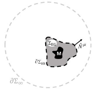
Figure 2: Schematic of the spacelike three-dimensional hypersurface $\Sigma_{\text{EG}}$ used in Ref. Verlinde2011, which has the mass under study embedded within it. As can be seen, the 2-surface corresponding to the holographic screen $\partial\Sigma_{\text{HS}}$ is now the outer boundary to $\Sigma_{\text{EG}}$ (compare to Fig. 1); and Ref. Verlinde2011, defines $\partial\Sigma_{\text{HS}}$ as ordinary surfaces of constant Newtonian potential $\phi$. (For context, we show spatial infinity as $\partial\Sigma_{\infty}$ in grey, though it plays no roll in this section.)

The ‘local’ temperature of the holographic screen (as measured at spatial infinity) used in Ref. Verlinde2011, is defined as

$$T\equiv\frac{1}{2\pi}e^{\phi}\,\phi_{;\mu}\hat{N}^{\mu},$$ (68)

where $\phi$ is the generalized Newtonian potential, given by $\phi=\frac{1}{2}\text{ln}(-K^{\mu}K_{\mu})=\ln{\cal N}$, recalling that $K^{\mu}K_{\mu}=-{\cal N}^{2}$. It is now an easy matter to check that

$$T \equiv \frac{1}{2\pi}e^{\phi}\,\phi_{;\mu}\hat{N}^{\mu}=\frac{1}{2\pi}{\cal N}_{;\mu}\hat{N}^{\mu}=\frac{1}{2\pi}\frac{1}{2{\cal N}}({\cal N}^{2})_{;\mu}\hat{N}^{\mu}$$ (69)

$$= -\frac{1}{2\pi}{K_{\nu}}_{;\mu}\frac{1}{\cal N}\,K^{\nu}\hat{N}^{\mu}=\frac{1}{2\pi}K_{\mu;\nu}\frac{1}{\cal N}\,K^{\nu}\hat{N}^{\mu}$$

$$= \frac{1}{2\pi}K_{\mu;\nu}\hat{T}^{\nu}\hat{N}^{\mu}.$$

In summary, recall the definition of $\kappa$ in Eq. (11), yielding

$$\boxed{T\equiv\frac{\kappa}{2\pi}.}$$ (70)

For reference, the Unruh temperature associated with a stationary observer is just the magnitude of the observer’s proper acceleration $a^{\mu}$ over $2\pi$. As their 4-velocity is given by $\hat{T}^{\mu}$ we easily find

$$a^{\mu}\equiv\hbox{${\hat{T}}^{\mu}$}_{;\nu}{\hat{T}}^{\nu}=\phi^{;\mu},$$ (71)

since ${\hat{T}}^{\mu}={\hat{T}}^{t}K^{\mu}=K^{\mu}/{\cal N}=e^{-\phi}K^{\mu}$. Thus $a^{\mu}$ is perpendicular to surfaces of constant $\phi$. When Verlinde’s temperature is measured locally (instead of referenced to spatial infinity) it is $T_{\text{local}}=\frac{1}{2\pi}\phi^{;\mu}{\hat{N}}_{\mu}$. For this to equal the Unruh temperature at the same point, the local unit normal ${\hat{N}}^{\mu}$ to the screen must be aligned with the proper acceleration $a^{\mu}$ of our stationary observer there. Therefore, it trivially follows that only for surfaces of constant Newtonian potential $\phi$ would the holographic screens be in thermal equilibrium with stationary physical surfaces of the same shape, size and location. Hence,

$$\boxed{\text{Thermodynamic equilibrium}\;\;\Rightarrow\;\;\hat{N}^{\mu}\parallel\phi^{;\mu}}$$ (72)

Finally, we show that for surfaces of constant $\phi$, we have $\delta\phi=k_{1}/2$. Indeed, since ${\hat{T}}^{t}=1/{\cal N}=e^{-\phi}$, we have

$$\boxed{\delta\phi=-\frac{1}{{\hat{T}}^{t}}\delta{\hat{T}}^{t}=\frac{1}{2}k_{1},}$$ (73)

where in the last step we have used Eqs. (40) and (41).

References

• (1) Bardeen, J. M., Carter, B. & Hawking, S. W. The four laws of black hole mechanics. Communications in Mathematical Physics 31, 161–170 (1973).
• (2) Hawking, S. W. Particle creation by black holes. Communications in mathematical physics 43, 199–220 (1975).
• (3) Unruh, W. G. Notes on black-hole evaporation Physical Review D 14, 870 (1976).
• (4) Jacobson, T. Thermodynamics of spacetime: The Einstein equation of state. Physical Review Letters 75, 1260 (1995).
• (5) Gibbons, G. W. & Hawking, S. W. Cosmological event horizons, thermodynamics, and particle creation. Physical Review D 15, 2738 (1977).
• (6) Thorne, K. S., Price, R. H. & Macdonald, D. A. Black Holes: The Membrane Paradigm (Yale University Press, Yale, 1986) pp.35-37.
• (7) Zurek, W. H. & Thorne, K. S. Statistical mechanical origin of the entropy of a rotating, charged black hole. Physical review letters 54, 2171 (1985).
• (8) Verlinde, E. On the Origin of Gravity and the Laws of Newton. Journal of High Energy Physics 2011, 29 (2011).
• (9) Hawking, S. W. & Ellis, G. F. R. The large scale structure of space-time. (Cambridge University Press, 1973), pp82-83, p334,.
• (10) Birkhoff, G. D. & Langer, R. E. Relativity and modern physics. (Cambridge, Harvard University Press, 1923).
• (11) Chen, Y.-X. & Li, J.-L. First law of thermodynamics on holographic screens in entropic force frame. Physics Letters B 700, 380–384 (2011).
• (12) Carroll, S. M. An Introduction to General Relativity Spacetime and Geometry (Addison Wesley, San Francisco, 2004). p251, p450, p456.
• (13) Gourgoulhon, E. 3+ 1 Formalism in General Relativity: Bases of Numerical Relativity (Springer Science & Business Media, 2012). pp79-84.
• (14) Bertschinger, E. Symmetry transformations, the Einstein-Hilbert action and gauge invariance. Massachusetts Institute of Technology, Department of Physics (2002).
• (15) Palatini, Attilio Deduzione invariantiva delle equazioni gravitazionali dal principio di Hamilton. Rendiconti del Circolo Matematico di Palermo (1884-1940) 43, 203–212 (1919).
• (16) Poisson, E. A relativist’s toolkit: the mathematics of black-hole mechanics. (Cambridge university press, 2004), p15, pp211-212.
• (17) Wald, R. M. General relativity. (University of Chicago press, 1984), p289, p336, p453, p463.
• (18) Piazza, F. Gauss-Codazzi thermodynamics on the timelike screen. Physical Review D 82, 084004 (2010).