Bregman Proximal Langevin Monte Carlo
via Bregman–Moreau Envelopes

Abstract

We propose efficient Langevin Monte Carlo algorithms for sampling distributions with nonsmooth convex composite potentials, which is the sum of a continuously differentiable function and a possibly nonsmooth function. We devise such algorithms leveraging recent advances in convex analysis and optimization methods involving Bregman divergences, namely the Bregman–Moreau envelopes and the Bregman proximity operators, and in the Langevin Monte Carlo algorithms reminiscent of mirror descent. The proposed algorithms extend existing Langevin Monte Carlo algorithms in two aspects—the ability to sample nonsmooth distributions with mirror descent-like algorithms, and the use of the more general Bregman–Moreau envelope in place of the Moreau envelope as a smooth approximation of the nonsmooth part of the potential. A particular case of the proposed scheme is reminiscent of the Bregman proximal gradient algorithm. The efficiency of the proposed methodology is illustrated with various sampling tasks at which existing Langevin Monte Carlo methods are known to perform poorly.

1 Introduction

The problem of sampling efficiently from high-dimensional log-Lipschitz-smooth and (strongly) log-concave target distributions via discretized Langevin diffusions has been extensively studied in the machine learning and statistics literature lately. A thorough understanding of the nonasymptotic convergence properties of Langevin Monte Carlo (LMC) has been developed, where the log-Lipschitz-smoothness and (strong) log-concavity of the density play a vital role in characterizing its convergence rates. However, such conditions are not always satisifed in applications and there is recent effort to move beyond such scenarios. On the other hand, since the efficiency of LMC algorithms in the stanard Euclidean space heavily hinges on the shape of the target distributions, algorithms based on Riemannian Langevin diffusions (Girolami and Calderhead, 2011) are considered in the case of ill-conditioned target distributions to exploit the local geometry of the log-density. However, algorithms derived by discretizing such Riemannian Langevin diffusions are notoriously hard to analyze, depending on the choice of the Riemannian metric.

In this paper, we propose two Riemannian LMC algorithms based on Bregman divergences to efficiently sample from high-dimensional distributions whose potentials (i.e., negative log-densities) are possibly not strongly convex nor (globally) Lipschitz smooth in the standard Euclidean geometry, but only strongly convex and Lipschitz smooth relative to a Legendre function subsequent to a smooth approximation. To be more precise, potentials can take the form of the sum of a relatively smooth part and a nonsmooth part (which includes the convex indicator function of a closed convex set) in the standard Euclidean geometry. A smooth approximation of the nonsmooth part based on the Bregman divergence is used and we instead sample from the smoothened distribution. By tuning a parameter of the smooth approximation, such a smoothened distribution is sufficiently close to the original target distribution. On the other hand, motivated by the connection between Langevin algorithms and convex optimization, the proposed algorithms can be viewed as the sampling analogue of the Bregman proximal gradient algorithm (Van Nguyen, 2017; Bauschke et al., 2017; Bolte et al., 2018; Bùi and Combettes, 2021; Chizat, 2021) (cf. mirror descent in the smooth case), in which Riemannian structures of the algorithms are induced by the Hessian of some Legendre function. This specific choice of the Riemannian metric also offers us a principled way to analyze the behavior of the proposed algorithms.

1.1 Langevin and Mirror-Langevin Monte Carlo Algorithms

We consider the problem of sampling from a probability measure $\pi$ on $(\mathbb{R}^{d},\mathcal{B}(\mathbb{R}^{d}))$ which admits a density, with slight abuse of notation, also denoted by $\pi$, with respect to the Lebesgue measure

$$(\forall x\in\mathbb{R}^{d})\quad\pi(x)=\left.\mathrm{e}^{-U(x)}\,\middle/\,\int_{\mathbb{R}^{d}}\mathrm{e}^{-U(y)}\,\mathrm{d}y\right.,$$ (1)

where the potential $U\colon\mathbb{R}^{d}\to\mathbb{R}\cup\{+\infty\}$ is measurable and we assume that $0<\int_{\mathcal{U}}\mathrm{e}^{-U(y)}\,\mathrm{d}y<+\infty$ for $\mathcal{U}\coloneqq\operatorname*{dom}U$. We also write $\pi\propto\mathrm{e}^{-U}$ for (1). Usually, the number of dimensions $d\gg 1$.

To perform such a sampling task, the LMC algorithm (see e.g., Dalalyan, 2017b) is arguably the most widely-studied gradient-based MCMC algorithm, which takes the form

$$(\forall k\in\mathbb{N})\quad x_{k+1}=x_{k}-\gamma\nabla U(x_{k})+\sqrt{2\gamma}\,\xi_{k},$$ (2)

where $\xi_{k}\stackrel{{\scriptstyle\text{i.i.d.}}}{{\sim}}\mathsf{N}_{d}(0,\mathsf{I}_{d})$ for all $k\in\mathbb{N}$ and $\gamma>0$ is a step size. Possibly with varying step sizes, the LMC algorithm is also referred to as the unadjusted Langevin algorithm (ULA; Durmus and Moulines, 2017) in the literature, while applying a Metropolis–Hastings correction step at each iteration of (2) the algorithm is often referred to as the Metropolis-adjusted Langevin algorithm (MALA; Roberts and Tweedie, 1996). ULA is the discretization of the overdamped Langevin diffusion, which is the solution to the stochastic differential equation (SDE)

$$(\forall t\in\left[0,+\infty\right[)\quad\mathrm{d}X_{t}=-\nabla U(X_{t})\,\mathrm{d}t+\sqrt{2}\,\mathrm{d}W_{t},$$ (3)

where $\{W_{t}\}_{t\in\left[0,+\infty\right[}$ is a $d$-dimensional standard Wiener process (a.k.a. Brownian motion). When $U$ is Lipschitz smooth and strongly convex, it is well known that $\pi$ has the unique invariant measure, which is the Gibbs measure $X_{\infty}\propto\mathrm{e}^{-U}$. Under such (or weaker) conditions of $U$, nonasymptotic error bounds of ULA in terms of various disimilarity measures of probability measures, e.g., total variation and Wasserstein distances, and KL, $\chi^{2}$- and Rényi divergences, are well studied and established (see e.g., Dalalyan, 2017a; Durmus and Moulines, 2017, 2019; Durmus et al., 2019; Vempala and Wibisono, 2019). To move beyond the Lipschitz smoothness assumption, we consider the case of a possibly nonsmooth composite potential $U$, which takes the following form

$$(\forall x\in\mathbb{R}^{d})\quad U(x)\coloneqq f(x)+g(x),$$ (4)

where $f\in\Gamma_{0}(\mathbb{R}^{d})$ is continuously differentiable but possibly not globally Lipschitz smooth (i.e., do not admit a globally Lipschitz gradient) and $g\in\Gamma_{0}(\mathbb{R}^{d})$ is possibly nonsmooth (see Section 1.4 for the definition of $\Gamma_{0}(\mathbb{R}^{d})$).

To demonstrate the sampling counterpart of mirror descent, we consider the smooth case (i.e., $g=0$) which is well studied in the literature. Introduced in Zhang et al. (2020), under certain assumptions on $U$, the mirror-Langevin diffusion (MLD) takes the form: for $t\in\left[0,+\infty\right[$,

$$\begin{cases}X_{t}=\nabla\varphi^{*}(Y_{t}),\\ \mathrm{d}Y_{t}=-\nabla U(X_{t})\,\mathrm{d}t+\sqrt{2}\left[\nabla^{2}\varphi(X_{t})\right]^{\nicefrac{{1}}{{2}}}\,\mathrm{d}W_{t},\end{cases}$$ (5)

where $\varphi$ is a Legendre function and $\varphi^{*}$ is the Fenchel conjugate of $\varphi$ (see Definition 2.2). An Euler–Maruyama discretization scheme yields the Hessian Riemannian LMC (HRLMC) algorithm: for $k\in\mathbb{N}$,

$$x_{k+1}=\nabla\varphi^{*}\Big{(}\nabla\varphi(x_{k})-\gamma\nabla U(x_{k})\left.+\sqrt{2\gamma}\left[\nabla^{2}\varphi(x_{k})\right]^{\nicefrac{{1}}{{2}}}\xi_{k}\right).$$ (6)

This is the main discretization scheme considered in Zhang et al. (2020) and an earlier draft of Hsieh et al. (2018), and further studied in Li et al. (2022), which is a specific instance of the Riemannian LMC reminiscent of the mirror descent algorithm. Ahn and Chewi (2021) consider an alternative discretization scheme motivated by the mirrorless mirror descent (Gunasekar et al., 2021), called the mirror-Langevin algorithm (MLA):

$$(\forall k\in\mathbb{N})\quad\begin{aligned} x_{k+\nicefrac{{1}}{{2}}}&=\nabla\varphi^{*}\left(\nabla\varphi(x_{k})-\gamma\nabla U(x_{k})\right),\\ x_{k+1}&=\nabla\varphi^{*}(Y_{\gamma_{k}}),\end{aligned}$$ (7)

where

$$\begin{cases}\mathrm{d}Y_{t}=\sqrt{2}\left[\nabla^{2}\varphi^{*}(Y_{t})\right]^{-\nicefrac{{1}}{{2}}}\,\mathrm{d}W_{t}\\ Y_{0}=\nabla\varphi\left(x_{k+\nicefrac{{1}}{{2}}}\right)=\nabla\varphi(x_{k})-\gamma\nabla U(x_{k}).\end{cases}$$ (8)

However, the mirror descent-type Langevin algorithms in Hsieh et al. (2018); Zhang et al. (2020); Ahn and Chewi (2021) can only handle relatively smooth potentials (to a Legendre function; see Definition 2.7) but not potentials with relatively smooth plus nonsmooth parts (4) where $g\neq 0$.

1.2 Contributions

We fill this void by extending HRLMC in the following aspects: (i) the target potential $U$ takes the form (4), i.e., $U=f+g$, where $f$ is continuously differentiable but possibly not Lipschitz smooth yet smooth relative to a Legendre function $\varphi$, and $g$ is possibly nonsmooth; (ii) the nonsmooth part $g$ is enveloped by its continuously differentiable approximation, which is the Bregman–Moreau envelope (Kan and Song, 2012; Bauschke et al., 2018; Laude et al., 2020; Soueycatt et al., 2020; Bauschke et al., 2006; Chen et al., 2012), in the same vein as using the Moreau envelope (Moreau, 1962, 1965) in Brosse et al. (2017); Durmus et al. (2018); Luu et al. (2021), so that we can adapt recent convergence results for mirror-Langevin algorithms for relatively smooth potentials (Zhang et al., 2020; Ahn and Chewi, 2021; Li et al., 2022; Jiang, 2021).

The proposed sampling algorithm can be viewed as a generalized version of the Moreau–Yosida Unadjusted Langevin Algorithm (MYULA; Durmus et al., 2018; Brosse et al., 2017), and we recover MYULA if both the mirror map and the Legendre function in the smooth approximation are chosen as $\nicefrac{{\|\cdot\|^{2}}}{{2}}$. Similar to the resemblance of MYULA to the proximal gradient algorithm with specific choice of step sizes, the proposed discretized algorithms is also reminiscent of the Bregman proximal gradient algorithm or the Bregman forward-backward algorithm (Van Nguyen, 2017; Bauschke et al., 2017; Bolte et al., 2018; Bùi and Combettes, 2021, see Section 3.3 for details). The proposed schemes, however, are able to change the geometry of the potential through a mirror map. On the theoretical front, our convergence results reveal a biased convergence guarantee with a bias which vanishes with the step size and the smoothing parameter of the Bregman–Moreau envelope. Numerical experiments also illustrate the efficiency of the proposed algorithms. We perform various nonsmooth (composite) and/or constrained sampling tasks, including sampling from the nonsmooth anisotropic Laplace distributions, at which MYULA is known to underperform ascribed to the anisotropy. To the best of our knowledge, the proposed algorithms are the first gradient-based Monte Carlo algorithms based on the overdamped Langevin dynamics which are able to sample nonsmooth composite distributions while adapting to the geometry of such distributions.

1.3 Related Work

1.3.1 Mirror Descent-Type Sampling Algorithms

In addition to Zhang et al. (2020); Ahn and Chewi (2021), Hsieh et al. (2018) introduce the mirrored-Langevin algorithm, which is also reminiscent of mirror descent, but only with $I_{d}$ instead of $\nabla^{2}\varphi$ in (5), which entails a standard Gaussian noise in (6). Their convergence guarantee is also based on the assumption that $\varphi$ is strongly convex. Chewi et al. (2020) analyze the continuous-time MLD (5) and specialize their results to the case when the mirror map is equal to the potential, known as the Newton–Langevin diffusion due to its resemblance to the Newton’s method in optimization. Li et al. (2022) improve upon the analysis of Zhang et al. (2020), establishing a vanishing bias with the step size of the mirror Langevin algorithm under more relaxed assumptions.

1.3.2 Nonsmooth Sampling

Sampling efficiently from nonsmooth distributions remains a crucial problem in machine learning, statistics and imaging sciences. In particular, a significant amount of work borrows tools from convex/variational analysis and proximal optimization, i.e., the Moreau envelope and proximity operator, attributing their use to the connection between sampling and optimization, see e.g., Pereyra (2016); Brosse et al. (2017); Bubeck et al. (2018); Durmus et al. (2019, 2018); Mou et al. (2019); Wibisono (2019); Luu et al. (2021); Lee et al. (2021); Lehec (2021); Liang and Chen (2021). Nonasymptotic convergence guarantees are generally obtained from the (Metropolis-adjusted) Langevin algorithms for smooth potentials. A notable exception which does not use the Moreau envelope as a smooth approximation is Chatterji et al. (2020), which applies Gaussian smoothing instead.

1.3.3 Bregman Divergences in Convex Analysis, Optimization and Machine Learning

The origin of convex analysis results involving Bregman divergences (Bregman, 1967) and related optimization methods date backs to more than four decades ago (see e.g., Bauschke and Borwein, 1997; Bauschke and Lewis, 2000; Bauschke et al., 2001; Bauschke and Borwein, 2001; Bauschke, 2003; Bauschke et al., 2003, 2006, 2009; Nemirovski, 1979; Nemirovski and Yudin, 1983). The work by Bauschke et al. (2017) is a major recent breakthrough which revives much interest in developing new optimization algorithms involving Bregman divergences and their convergence results (see e.g., Bùi and Combettes, 2021; Bolte et al., 2018; Bauschke et al., 2019; Dragomir et al., 2021b, a; Hanzely et al., 2021; Teboulle, 2018; Takahashi et al., 2021; Chizat, 2021). Bauschke et al. (2017) relax the globally Lipschitz gradient assumption commonly required in gradient descent or proximal gradient for convergence, by introducing the relative smoothness condition (Definition 2.7). Our proposed sampling algorithms also rely on such an insightful condition. Another long line of work studies the generalization of the notions of the classical Moreau envelope and the proximity operators (Moreau, 1962, 1965; Rockafellar and Wets, 1998; Bauschke and Combettes, 2017) in convex analysis using Bregman divergences, see e.g., Bauschke et al. (2003, 2006); Chen et al. (2012); Kan and Song (2012); Bauschke et al. (2018); Laude et al. (2020); Soueycatt et al. (2020). This line of work motivates our use of the Bregman–Moreau envelopes as smooth approximations of the nonsmooth part of the potential. While there is an extensive amount of literature regarding the applications of Bregman divergences in machine learning other than mirror descent (Bubeck, 2015), we refer to Blondel et al. (2020) which includes useful results for sampling distributions on various convex polytopes such as the probability simplex based on our proposed schemes.

1.4 Notation

We denote by $I_{d}\in\mathbb{R}^{d\times d}$ the $d\times d$ identity matrix. We also define $\overline{\mathbb{R}}\coloneqq\mathbb{R}\cup\{+\infty\}$. Let $\mathbb{S}^{d}_{++}$ denote the set of symmetric positive definite matrices of $\mathbb{R}^{d\times d}$. Let $\mathcal{H}$ be a real Hilbert space endowed with an inner product $\left\langle\cdot,\cdot\right\rangle$ and a norm $\|\cdot\|$. The domain of a function $f\colon\mathcal{H}\to\overline{\mathbb{R}}$ is $\operatorname*{dom}f\coloneqq\{x\in\mathcal{H}:f(x)<+\infty\}$. The set $\Gamma_{0}(\mathbb{R}^{d})$ denotes the class of lower-semicontinuous convex functions from $\mathbb{R}^{d}$ to $\overline{\mathbb{R}}$ with a nonempty domain (i.e., proper). The convex indicator function $\iota_{\mathcal{C}}(x)$ of a closed convex set $\mathcal{C}\neq\varnothing$ at $x$ equals $0$ if $x\in\mathcal{C}$ and $+\infty$ otherwise. We denote by $\mathcal{B}(\mathbb{R}^{d})$ the Borel $\sigma$-field of $\mathbb{R}^{d}$. For two probability measures $\mu$ and $\nu$ on $\mathcal{B}(\mathbb{R}^{d})$, the total variation distance between $\mu$ and $\nu$ is defined by $\|\mu-\nu\|_{\mathrm{TV}}=\sup_{\mathsf{A}\in\mathcal{B}(\mathbb{R}^{d})}|\mu(\mathsf{A})-\nu(\mathsf{A})|$. For $k\in\mathbb{N}$, we denote by $\mathscr{C}^{k}$ the set of $k$-times continuously differentiable functions $f\colon\mathbb{R}^{d}\to\mathbb{R}$. If $f$ is a Lipschitz function, i.e., there exists $L>0$ such that for all $x,y\in\mathbb{R}^{d}$, $|f(x)-f(y)|\leqslant L\|x-y\|$, then we denote $\|f\|_{\mathrm{Lip}}\coloneqq\inf\{|f(x)-f(y)|/\|x-y\|\,|\,x,y\in\mathbb{R}^{d},x\neq y\}$.

2 Preliminaries

In this section, we give definitions of important notions from convex analysis (Rockafellar, 1970; Rockafellar and Wets, 1998; Bauschke and Combettes, 2017), and state some related properties of such notions. In this section, we let $\varphi\in\Gamma_{0}(\mathbb{R}^{d})$ and $\mathcal{X}\coloneqq\operatorname*{int}\operatorname*{dom}\varphi$.

Definition 2.1 (Legendre functions).

A function $\varphi$ is called (i) essentially smooth, if it is differentiable on $\mathcal{X}\neq\varnothing$ and $\|\nabla\varphi(x_{n})\|\to+\infty$ whenever $x_{n}\to x\in\operatorname{bdry}\operatorname*{dom}\varphi$ ; (ii) essentially strictly convex, if it is strictly convex on $\mathcal{X}$; (iii) Legendre, if it is both essentially smooth and essentially strictly convex.

Definition 2.2 (Fenchel conjugate).

The Fenchel conjugate of a proper function $f$ is defined by $f^{*}(x)\coloneqq\sup_{y\in\mathbb{R}^{d}}\,\left\{\left\langle y,x\right\rangle-f(y)\right\}$. For a Legendre function $\varphi$, it is well known that $\nabla\varphi\colon\mathcal{X}\to\mathcal{X}^{*}\coloneqq\operatorname*{int}\operatorname*{dom}\varphi^{*}$ with $(\nabla\varphi)^{-1}=\nabla\varphi^{*}$.

Definition 2.3 (Bregman divergence).

The Bregman divergence between $x$ and $y$ associated with a Legendre function $\varphi$ is defined through

$$D_{\varphi}\colon\mathbb{R}^{d}\times\mathbb{R}^{d}\to[0,+\infty]\colon(x,y)\mapsto\begin{cases*}\varphi(x)-\varphi(y)-\left\langle\nabla\varphi(y),x-y\right\rangle,&if $y\in\mathcal{X}$,\\ +\infty,&otherwise.\end{cases*}$$ (9)

We now assume that $\varphi$ is a Legendre function in the remaining part of this section.

Definition 2.4 (Bregman–Moreau envelopes).

For $\lambda>0$, the left and right Bregman–Moreau envelopes of $g\in\Gamma_{0}(\mathbb{R}^{d})$ associated with $\varphi$ are respectively defined by

$$\overleftarrow{\mathrm{env}}_{\lambda,g}^{\varphi}(x)\coloneqq\inf_{y\in\mathbb{R}^{d}}\,\left\{g(y)+\frac{1}{\lambda}D_{\varphi}(y,x)\right\},$$ (10)

and

$$\overrightarrow{\mathrm{env}}_{\lambda,g}^{\varphi}(x)\coloneqq\inf_{y\in\mathbb{R}^{d}}\,\left\{g(y)+\frac{1}{\lambda}D_{\varphi}(x,y)\right\}.$$ (11)

Definition 2.5 (Bregman proximity operators).

For $\lambda>0$, the left and right Bregman proximity operators of $g\in\Gamma_{0}(\mathbb{R}^{d})$ associated with $\varphi$ are respectively defined by

$$\overleftarrow{\operatorname{P}}_{\negthinspace\negthinspace\lambda,g}^{\varphi}(x)\coloneqq\operatorname*{argmin}_{y\in\mathbb{R}^{d}}\,\left\{g(y)+\frac{1}{\lambda}D_{\varphi}(y,x)\right\},$$ (12)

and

$$\overrightarrow{\operatorname{P}}_{\negthinspace\negthinspace\lambda,g}^{\varphi}(x)\coloneqq\operatorname*{argmin}_{y\in\mathbb{R}^{d}}\,\left\{g(y)+\frac{1}{\lambda}D_{\varphi}(x,y)\right\}.$$ (13)

We omit the arrows and write $\mathrm{env}_{\lambda,g}^{\varphi}$ and $\operatorname{P}_{\negthinspace\negthinspace\lambda,g}^{\varphi}$ when there is no need to distinguish the left and right Bregman–Moreau envelopes or Bregman proximity operators. When $\varphi=\nicefrac{{\|\cdot\|^{2}}}{{2}}$, we recover the classical Moreau envelope and the Moreau proximity operator (Moreau, 1962, 1965). Note that $\mathrm{env}_{\lambda,g}^{\varphi}$ envelops $g$ from below and is decreasing in $\lambda$, in a sense that $\inf g(\mathbb{R}^{d})\leqslant\mathrm{env}_{\lambda,g}^{\varphi}(x)\leqslant\mathrm{env}_{\kappa,g}^{\varphi}(x)\leqslant g(x)$ for any $x\in\mathcal{X}$ and $0<\kappa<\lambda<+\infty$ (Bauschke et al., 2018, Proposition 2.2).

Definition 2.6 (Legendre strongly convex).

A function $f$ is $\alpha$-Legendre strongly convex with respect to $\varphi$ if there exists a constant $\alpha\geqslant 0$ such that $f-\alpha\varphi$ is convex on $\mathcal{X}$.

Definition 2.7 (Relative smoothness).

A function $f$ is $\beta$-smooth relative to $\varphi$ if there exists $\beta>0$ such that $\beta\varphi-f$ is convex on $\mathcal{X}$.

3 Bregman Proximal LMC Algorithms

In the case of nonsmooth composite potentials, the mirror-Langevin algorithms (6) and (7) no longer work since the gradient of the nonsmooth part is not available. Based on the mirror Langevin algorithms for relatively smooth potentials (Zhang et al., 2020; Ahn and Chewi, 2021), we devise two possible Bregman proximal LMC algorithms involving the Bregman–Moreau envelopes and the Bregman proximity operators.

3.1 Assumptions and Related Properties

Instead of directly sampling from $\pi$, we propose to sample from distributions whose potentials being smooth surrogates of $U$, defined by

$$\overleftarrow{U}_{\negthinspace\negthinspace\lambda}^{\psi}\coloneqq f+\overleftarrow{\mathrm{env}}_{\lambda,g}^{\psi}\quad\text{and}\quad\overrightarrow{U}_{\negthinspace\negthinspace\lambda}^{\psi}\coloneqq f+\overrightarrow{\mathrm{env}}_{\lambda,g}^{\psi},$$ (14)

where $\psi\in\Gamma_{0}(\mathbb{R}^{d})$ is a Legendre function possibly different from the Legendre function $\varphi$ in MLD (5) to allow full flexibility, and $\lambda>0$. Then the corresponding surrogate target densities are

$$\overleftarrow{\pi}_{\negthinspace\negthinspace\lambda}^{\psi}\propto\exp\left(-\overleftarrow{U}_{\negthinspace\negthinspace\lambda}^{\psi}\right)\quad\text{and}\quad\overrightarrow{\pi}_{\negthinspace\negthinspace\lambda}^{\psi}\propto\exp\left(-\overrightarrow{U}_{\negthinspace\negthinspace\lambda}^{\psi}\right).$$ (15)

We again omit the arrows and write $U_{\lambda}^{\psi}$ and $\pi_{\lambda}^{\psi}$ when we do not need to distinguish the left and right Bregman–Moreau envelopes. In this section, after introducing some required assumptions, we show that they are well-defined (i.e., in $\left]0,+\infty\right[$), as close to $\pi$ by adjusting the (sufficiently small) approximation parameter $\lambda>0$, Legendre strongly log-concave, and relatively smooth. We also give some extra assumptions of the specific algorithms (Assumption 3.8). Then, with all the assumptions of algorithms originally designed for the relatively smooth potentials satisfied by (14), we enable the capabilities of these algorithms for approximate nonsmooth sampling.

We write $\mathcal{F}\coloneqq\operatorname*{dom}f\subseteq\mathbb{R}^{d}$ and $\mathcal{G}\coloneqq\operatorname*{dom}g\subseteq\mathbb{R}^{d}$. Throughout the whole paper, we assume that $\mathcal{X}\coloneqq\operatorname*{int}\operatorname*{dom}\varphi$ and $\mathcal{Y}\coloneqq\operatorname*{int}\operatorname*{dom}\psi$ such that $(\operatorname*{int}\mathcal{F})\cap\mathcal{Y}\subseteq\overline{\mathcal{X}}$, $(\operatorname*{int}\mathcal{F})\cap\mathcal{Y}\cap\mathcal{X}\neq\varnothing$ and $\mathcal{G}\cap\mathcal{Y}\neq\varnothing$. Let us recall that the potential $U$ has the form $f+g$. We make the following assumptions on the functions $f$ and $g$, the Legendre functions $\varphi$ and $\psi$, and their associated Bregman divergences $D_{\varphi}$ and $D_{\psi}$.

Assumption 3.1.

The function $f\colon\mathbb{R}^{d}\to\mathbb{R}$ is (i) in $\Gamma_{0}(\mathbb{R}^{d})$, lower bounded and differentiable (i.e., of $\mathscr{C}^{1}$) but may not admit a globally Lipschitz gradient; (ii) $\beta_{f}$-smooth relative to $\varphi$.

Assumption 3.2.

The function $g\colon\mathbb{R}^{d}\to\overline{\mathbb{R}}$ is (i) in $\Gamma_{0}(\mathbb{R}^{d})$, lower bounded and possibly nonsmooth; either (ii^†) such that $\mathrm{e}^{-g}$ is integrable with respect to the Lebesgue measure, or (ii^‡) Lipschitz.

Assumption 3.3.

The function $\varphi\in\Gamma_{0}(\mathbb{R}^{d})$ is (i) Legendre; (ii) of $\mathscr{C}^{3}$ on $\mathcal{X}$; (iii) supercoercive, i.e., $\lim_{\|x\|\to+\infty}\varphi(x)/\|x\|=+\infty$; (iv) $M_{\varphi}$-modified self-concordant (Zhang et al., 2020; Li et al., 2022, (A1)), i.e., there exists $M_{\varphi}\in\left[0,+\infty\right[$ such that for any $(x,\widetilde{x})\in\mathcal{X}\times\mathcal{X}$, $\left|\kern-1.07639pt\left|\kern-1.07639pt\left|(\nabla^{2}\varphi(x))^{\nicefrac{{1}}{{2}}}-(\nabla^{2}\varphi(\widetilde{x}))^{\nicefrac{{1}}{{2}}}\right|\kern-1.07639pt\right|\kern-1.07639pt\right|_{\mathrm{F}}\leqslant\sqrt{M_{\varphi}}\left\lVert\nabla\varphi(x)-\nabla\varphi(\widetilde{x})\right\rVert$, where $|\kern-1.07639pt|\kern-1.07639pt|\cdot|\kern-1.07639pt|\kern-1.07639pt|_{{\mathrm{F}}}$ is the Frobenius norm. (v) very strictly convex, i.e., $\nabla^{2}\varphi(x)\in\mathbb{S}^{d}_{++}$ for all $x\in\mathcal{X}\neq\varnothing$ (Bauschke and Lewis, 2000).

Assumption 3.4.

The function $\psi\in\Gamma_{0}(\mathbb{R}^{d})$ is (i) Legendre; (ii) of $\mathscr{C}^{3}$ on $\mathcal{Y}$; (iii) supercoercive.

Assumption 3.5.

The Bregman divergence associated with $\psi$ satisfy the following assumptions: (i) $D_{\psi}$ is jointly convex, i.e., convex on $\mathbb{R}^{d}\times\mathbb{R}^{d}$; (ii) $(\forall y\in\mathcal{Y})\;D_{\psi}(y,\cdot)$ is strictly convex on $\mathcal{Y}$, continuous on $\mathcal{Y}$, and coercive, i.e., $(\forall y\in\mathcal{Y})\;D_{\psi}(y,z)\to+\infty$ as $\|z\|\to+\infty$.

Assumptions 3.1, 3.2, 3.3 and 3.4 are required for the convergence of the proposed algorithms. Assumption 3.2(ii) is required for (15) to be well-defined. Assumption 3.5 consists of the standard assumptions required for the well-posedness of the Bregman–Moreau envelopes and the Bregman proximity operators of $\psi$ (Bauschke et al., 2018). Proposition 3.6 below implies that the densities (15) are well-defined and as close to the target density $\pi$ as required when $\lambda$ is sufficiently small (in total variation distance). We also provide a computable error bound when evaluating exactly the expectation with respect to (15) as opposed to the true target distribution $\pi$.

Proposition 3.6.

Suppose that Assumptions 3.1, 3.2, 3.4 and 3.5 hold. Then the following statements hold.

1. Let $\lambda>0$. If either (i) Assumption 3.2(ii^†) holds or (ii) Assumption 3.2(ii^‡) holds and $\psi$ is $\rho$-strongly convex, then $\overleftarrow{\pi}_{\negthinspace\negthinspace\lambda}^{\psi}$ and $\overrightarrow{\pi}_{\negthinspace\negthinspace\lambda}^{\psi}$ define proper densities of probability measures on $\mathbb{R}^{d}$, i.e., $\exp\left(-\overleftarrow{U}_{\negthinspace\negthinspace\lambda}^{\psi}\right)$ and $\exp\left(-\overrightarrow{U}_{\negthinspace\negthinspace\lambda}^{\psi}\right)$ are integrable w.r.t. the Lebesgue measure.

2. $\pi_{\lambda}^{\psi}$ converges to $\pi$ as $\lambda\downarrow 0$, i.e., $\|\pi_{\lambda}^{\psi}-\pi\|_{\mathrm{TV}}\to 0$ as $\lambda\downarrow 0$.

3. If Assumption 3.2(ii^‡) holds and $\psi$ is $\rho$-strongly convex, then for all $\lambda>0$, $\|\pi_{\lambda}^{\psi}-\pi\|_{\mathrm{TV}}\leqslant\lambda\|g\|_{\mathrm{Lip}}^{2}/\rho$. In addition, for any $\pi$- and $\pi_{\lambda}^{\psi}$-integrable function $h\colon\mathbb{R}^{d}\to\mathbb{R}$,

   $$\left|\mathbb{E}_{\pi_{\lambda}^{\psi}}h-\mathbb{E}_{\pi}h\right|\leqslant\left(\mathrm{e}^{\lambda\|g\|_{\mathrm{Lip}}^{2}/\rho}-1\right)\cdot\min\left\{\mathbb{E}_{\pi_{\lambda}^{\psi}}|h|,\mathbb{E}_{\pi}|h|\right\}.$$

All proofs are postponed to Appendix A. Next we show that the surrogate potentials (14) are indeed continuously differentiable approximations of $U$ under certain conditions. Their gradients and the conditions for them to be Lipschitz are also given. We also assert that the Bregman–Moreau envelopes $\mathrm{env}_{\lambda,g}^{\psi}(y)$ have desirable asymptotic behavior as $\lambda$ goes to $0$.

Proposition 3.7.

Suppose that Assumptions 3.2, 3.4 and 3.5 hold and $\lambda>0$. The following statements hold.

1. The left and right Bregman–Moreau envelopes are differentiable on $\mathcal{Y}$ and

   $$\nabla\overleftarrow{\mathrm{env}}_{\lambda,g}^{\psi}(y)=\frac{1}{\lambda}\nabla^{2}\psi(y)\left(y-\overleftarrow{\operatorname{P}}_{\negthinspace\negthinspace\lambda,g}^{\psi}(y)\right),$$ (16)

   and

   $$\nabla\overrightarrow{\mathrm{env}}_{\lambda,g}^{\psi}(y)=\frac{1}{\lambda}\left(\nabla\psi(y)-\nabla\psi\left(\overrightarrow{\operatorname{P}}_{\negthinspace\negthinspace\lambda,g}^{\psi}(y)\right)\right),$$ (17)

   for any $y\in\mathcal{Y}$, respectively.

2. If $D_{\psi}(y,\cdot)$ is continuous and convex on $\mathcal{Y}$ for all $y\in\mathcal{Y}$, and $\nabla\psi$ is Lipschitz on $\mathcal{Y}$, then $\nabla\overleftarrow{\mathrm{env}}_{\lambda,g}^{\psi}$ and $\nabla\overrightarrow{\mathrm{env}}_{\lambda,g}^{\psi}$ are Lipschitz on $\mathcal{Y}$.

3. As $\lambda\downarrow 0$, we have $\overleftarrow{\mathrm{env}}_{\lambda,g}^{\psi}(y)\uparrow g(y)$ and $\overrightarrow{\mathrm{env}}_{\lambda,g}^{\psi}(y)\uparrow g(y)$ for all $y\in\mathcal{Y}$.

Finally, we make the following extra assumptions on $U_{\lambda}^{\psi}$, $\varphi$ and $\psi$.

Assumption 3.8.

We assume the following: For $\lambda>0$, (i) $\overleftarrow{U}_{\negthinspace\negthinspace\lambda}^{\psi}$ and $\overrightarrow{U}_{\negthinspace\negthinspace\lambda}^{\psi}$ are $\alpha$-Legendre strongly convex with respect to $\varphi$; (ii) $\overleftarrow{\mathrm{env}}_{\lambda,g}^{\psi}$ and $\overrightarrow{\mathrm{env}}_{\lambda,g}^{\psi}$ are $\beta_{g}$-smooth relative to $\varphi$.

Assumption 3.8 is a set of rather generic assumptions but gives us guidance to choose $\psi$ and $\varphi$. Note that if $f$ is $\alpha$-Legendre strongly convex with respect to $\varphi$, then Assumption 3.8(i) is automatically satisfied. Also note that the constants $\alpha$ and $\beta_{g}$ can be different for the left and right versions of their corresponding quantities.

Remark 3.9.

Let us define $\beta\coloneqq\beta_{f}+\beta_{g}$. Assumption 3.1(iv) and Assumption 3.8(ii) implies $U_{\lambda}^{\psi}$ is $\beta$-smooth relative to $\varphi$. Then, $U_{\lambda}^{\psi}$ satisfies (A2) and (A3) of Li et al. (2022), which are required for the convergence of HRLMC.

We propose two mirror-Langevin algorithms which use different discretizations of the mirror-Langevin diffusion. We give the details of the algorithm based on HRLMC in the main text. The algorithm based on MLA, which is essentially (7) with $U$ replaced by $U_{\lambda}^{\psi}$, coined the Bregman–Moreau mirrorless mirror-Langevin algorithm (BMMMLA), is given in Appendix C.

3.2 The Bregman–Moreau Unadjusted Mirror-Langevin Algorithm

Let $x_{0}\in\mathcal{Y}$. A discretization scheme for the case of composite potentials similar to HRLMC (6), called the Bregman–Moreau unadjusted mirror-Langevin algorithm (BMUMLA), iterates, for $k\in\mathbb{N}$,

$$x_{k+1}=\nabla\varphi^{*}\Big{(}\nabla\varphi(x_{k})-\gamma\nabla U_{\lambda}^{\psi}(x_{k})\left.+\sqrt{2\gamma}\left[\nabla^{2}\varphi(x_{k})\right]^{\nicefrac{{1}}{{2}}}\xi_{k}\right).$$ (18)

More specifically, when $\varphi=\psi=\nicefrac{{\left\lVert\cdot\right\rVert^{2}}}{{2}}$, then we have $\nabla\varphi=\mathrm{Id}$, $\nabla\varphi^{*}=(\nabla\varphi)^{-1}=\mathrm{Id}$, $\nabla^{2}\varphi=I_{d}$, and $\left(\nabla\varphi+\lambda\partial g\right)^{-1}=(\mathrm{Id}+\lambda\partial g)^{-1}=\operatorname{prox}_{\lambda g}$, so that BMUMLA (18) reduces to MYULA (Durmus et al., 2018). Furthermore, letting $y_{k}=\nabla\varphi(x_{k})$ for all $k\in\mathbb{N}$, then the BMUMLA in the dual space $\nabla\varphi(\mathcal{X})$ takes the form

$$y_{k+1}=y_{k}-\gamma\nabla U_{\lambda}^{\psi}\circ\nabla\varphi^{*}(y_{k})+\sqrt{2\gamma}\left[\nabla^{2}\varphi^{*}(y_{k})\right]^{\nicefrac{{1}}{{2}}}\xi_{k}.$$ (19)

Recent results by Li et al. (2022) show that HRLMC indeed has a vanishing bias with the step size $\gamma$, as opposed to what was conjectured in Zhang et al. (2020). An advantage of applying HRLMC over MLA is that an exact simulator of the Brownian motion of varying covariance is not needed, which is usually approximated by inner loops of Euler–Maruyama discretization in practice (Ahn and Chewi, 2021). It is however worth noting that the use of the Bregman–Moreau envelope still incurs bias in our proposed algorithms, but can be controlled via the smoothing parameter $\lambda$ (see Section 4).

3.3 Reminiscence of Bregman Proximal Gradient Algorithm via Right BMUMLA

The proposed BMUMLA can be simplified by specifying $\psi=\varphi$, regarding the iterates and the assumptions. In particular, the right BMUMLA reduces to

$$\nabla\varphi\left(x_{k+1}\right)=\left(1-\frac{\gamma}{\lambda}\right)\nabla\varphi(x_{k})-\gamma\nabla f(x_{k})+\frac{\gamma}{\lambda}\nabla\varphi\left(\overrightarrow{\operatorname{P}}_{\negthinspace\negthinspace\lambda,g}^{\varphi}(x_{k})\right)+\sqrt{2\gamma}\left[\nabla^{2}\varphi(x_{k})\right]^{\nicefrac{{1}}{{2}}}\xi_{k},$$ (20)

which can be viewed as the generalization of MYULA (Durmus et al., 2018) with the right Bregman–Moreau envelope, but with a diffusion term of varying covariance. Furthermore, if we let $\gamma=\lambda$, then (20) becomes

$$x_{k+1}=\nabla\varphi^{*}\left(\nabla\varphi\left(\overrightarrow{\operatorname{P}}_{\negthinspace\negthinspace\lambda,g}^{\varphi}(x_{k})\right)-\lambda\nabla f(x_{k})+\sqrt{2\gamma}\left[\nabla^{2}\varphi(x_{k})\right]^{\nicefrac{{1}}{{2}}}\xi_{k}\right),$$ (21)

which roughly resembles the iterates of the Bregman proximal gradient algorithm (Van Nguyen, 2017; Bauschke et al., 2017; Bolte et al., 2018; Bùi and Combettes, 2021; Chizat, 2021), which takes the form

$$x_{k+1}=\overleftarrow{\operatorname{P}}_{\negthinspace\negthinspace\lambda,g}^{\varphi}\left(\nabla\varphi^{*}\left(\nabla\varphi(x_{k})-\lambda\nabla f(x_{k})\right)\right),$$ (22)

or

$$z_{k+1}=\nabla\varphi^{*}\left(\nabla\varphi\left(\overleftarrow{\operatorname{P}}_{\negthinspace\negthinspace\lambda,g}^{\varphi}(z_{k})\right)-\lambda\nabla f\left(\overleftarrow{\operatorname{P}}_{\negthinspace\negthinspace\lambda,g}^{\varphi}(z_{k})\right)\right),$$ (23)

if we write $z_{k}=\nabla\varphi^{*}\left(\nabla\varphi(x_{k})-\lambda\nabla f(x_{k})\right)$. The differences between (23) and (21), other than the diffusion term, are the use of different Bregman–Moreau envelopes and the argument of the gradient of the smooth part.

Another advantage of using the same mirror map is that Assumption 3.8 can be made more precise. In particular, regarding Assumption 3.8(ii), since $\overrightarrow{\mathrm{env}}_{\lambda,g}^{\varphi}$ is $\lambda^{-1}$-smooth relative to $\varphi$ (Laude et al., 2020, Proposition 3.8(ii)), for the right BMUMLA with $\psi=\varphi$, i.e., (20), Assumption 3.8(ii) is made precise with a relative smoothness constant $\beta_{g}=\lambda^{-1}$ for $\overrightarrow{\mathrm{env}}_{\lambda,g}^{\varphi}$.

4 Convergence Analysis

We now state the main convergence results derived from Li et al. (2022). To quantify the convergence, we introduce a modified Wasserstein distance previously introduced by Zhang et al. (2020) and further applied in the analysis of Li et al. (2022).

Definition 4.1.

For two probability measures $\mu$ and $\nu$ on $\mathcal{B}(\mathcal{X})$, the (squared) modified Wasserstein distance under the mirror map $\nabla\varphi$ from $\mu$ to $\nu$ is defined by

$$\mathsf{W}_{2,\varphi}^{2}(\mu,\nu)\coloneqq\inf_{u\sim\mu,v\sim\nu}\mathbb{E}\left[\|\nabla\varphi(u)-\nabla\varphi(v)\|^{2}\right].$$

Note that if $\widetilde{\mu}\coloneqq(\nabla\varphi)_{\sharp}\mu$ and $\widetilde{\nu}\coloneqq(\nabla\varphi)_{\sharp}\nu$ are the pushforward measures of $\mu$ and $\nu$ by $\nabla\varphi$ respectively, then $\mathsf{W}_{2,\varphi}^{2}(\mu,\nu)=\mathsf{W}_{2}^{2}(\widetilde{\mu},\widetilde{\nu})\coloneqq\inf_{\widetilde{u}\sim\widetilde{\mu},\widetilde{v}\sim\widetilde{\nu}}\mathbb{E}\left[\|\widetilde{u}-\widetilde{v}\|^{2}\right]$.

The main convergence result is given as follows.

Theorem 4.2.

Let Assumptions 3.1, 3.2, 3.3, 3.4, 3.5 and 3.8 hold and $M_{\varphi}<\alpha/2$. Let $x_{k}\sim\mu_{k}$ be the iterates of (18) with step size $\gamma\in\left]0,\gamma_{\max}\right]$, where $\gamma_{\max}=\mathcal{O}\left((\alpha-2M_{\varphi})^{2}/\left(\beta^{2}(1+8M_{\varphi})^{2}\right)\right)$. Then, from any $x_{0}\sim\mu_{0}$, we have

$$\mathsf{W}_{2,\varphi}(\mu_{k},\pi_{\lambda}^{\psi})\leqslant\sqrt{2}\mathrm{e}^{-(\alpha-2M_{\varphi})\gamma k}\mathsf{W}_{2,\varphi}(\mu_{0},\pi_{\lambda}^{\psi})+C\sqrt{2\gamma},$$ (24)

where $C=\mathcal{O}\left(\beta(1+8M_{\varphi})\sqrt{d}/(\alpha-2M_{\varphi})\right)$ is a constant. Furthermore, if the stronger Assumption 3.2(ii^‡) rather than (ii^†) holds and $\psi$ is $\rho$-strongly convex, then

$$\mathsf{W}_{2,\varphi}(\mu_{k},\pi)\leqslant\sqrt{2}\mathrm{e}^{-(\alpha-2M_{\varphi})\gamma k}\mathsf{W}_{2,\varphi}(\mu_{0},\pi)+C\sqrt{2\gamma}+\left(1+\sqrt{2}\mathrm{e}^{-(\alpha-2M_{\varphi})\gamma k}\right)\frac{\eta\lambda}{\rho}\|g\|_{\mathrm{Lip}}^{2},$$ (25)

where $\eta\coloneqq\sup_{(u,v)\in\mathcal{X}\times\mathcal{X}}\|\nabla\varphi(u)-\nabla\varphi(v)\|^{2}$.

From Theorem 4.2, we can derive a mixing time bound for (18) similar to Corollary 3.2 of Li et al. (2022).

Corollary 4.3.

Suppose that Assumptions 3.1, 3.3, 3.4, 3.5 and 3.8 and Assumption 3.2(ii^‡) rather than (ii^†) hold, $\psi$ is $\rho$-strongly convex, and $M_{\varphi}<\alpha/2$. Then, for any target accuracy $\varepsilon>0$, in order to achieve $\mathsf{W}_{2}(\widetilde{\mu}_{k},\widetilde{\pi})\leqslant\varepsilon$, it suffices to run BMUMLA in the dual space (19) with step size $\gamma=\varepsilon^{2}/(18C^{2})$ and smoothing parameter $\lambda=\rho\varepsilon/(3\widetilde{\eta}\|g\|_{\mathrm{Lip}}^{2})$ for $k$ iterations, where

$$k\geqslant\frac{1}{(\alpha-2M_{\varphi})\gamma}\log\left(\frac{3\sqrt{2}[\mathsf{W}_{2}(\widetilde{\mu}_{0},\widetilde{\pi}_{\lambda}^{\psi})+\widetilde{\eta}\lambda\|g\|_{\mathrm{Lip}}^{2}/\rho]}{\varepsilon}\right)=\widetilde{\mathcal{O}}\left(\frac{\beta^{2}(1+8M_{\varphi})^{2}d}{(\alpha-2M_{\varphi})^{3}\varepsilon^{2}}\right),$$ (26)

where $\widetilde{\eta}\coloneqq\sup_{(u,v)\in\mathcal{X}\times\mathcal{X}}\|u-v\|^{2}$.

Assuming all other constants including $\alpha$, $\beta$, $M_{\varphi}$, $\eta$, $\rho$ and $\|g\|_{\mathrm{Lip}}$ are independent of $d$, then, similar to Li et al. (2022) for the relatively smooth case, (18) has a biased convergence guarantee with a bias incurred by the algorithm which scales as $\mathcal{O}(\sqrt{d\gamma})$. Since essentially we are sampling from the surrogate distribution $\pi_{\lambda}^{\psi}$ which is different from $\pi$, this incurs an additional bias. From (25), this bias attributed to smoothing with the Bregman–Moreau envelope scales as $\mathcal{O}(\lambda)$ for large enough $k$ and $\eta<+\infty$. We then obtain the same mixing time bound of $\widetilde{\mathcal{O}}(d/\varepsilon^{2})$ for BMUMLA as the one for MLA in Li et al. (2022). Note that the appearance of $\eta$ limits the choice of mirror maps in (18) as some choices of $\varphi$ might not give a bounded $\eta$ (see Jiang, 2021, for related discussion).

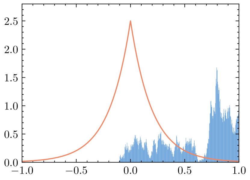
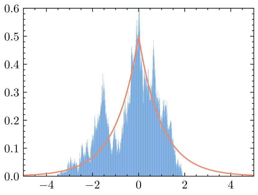
(a) 1^st dimension

(b) 2^nd dimension

(c) 5^th dimension

(d) 10^th dimension

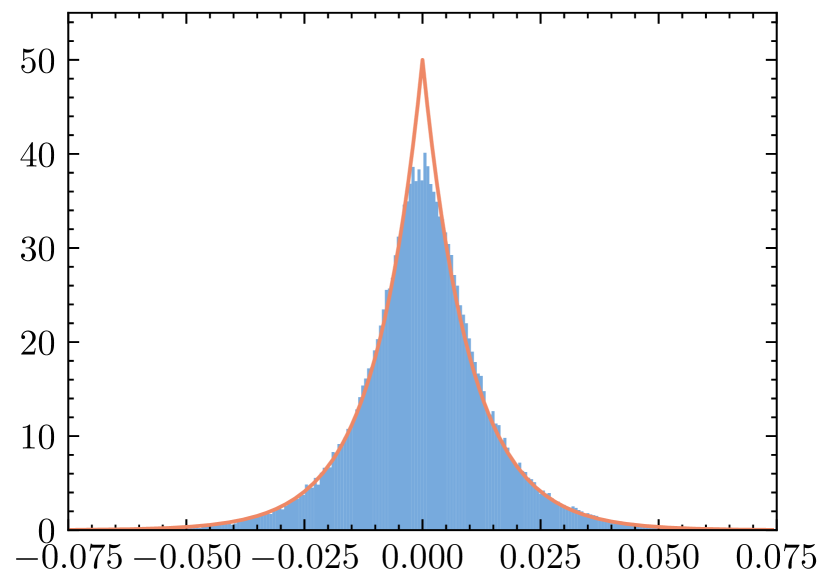
(e) 100^th dimension

Figure 1: Histograms of samples (blue) from MYULA (1^st row), BMUMLA (2^nd row) and the true densities (orange).

5 Numerical Experiments

We perform numerical experiments of sampling anisotropic Laplace distributions which have nonsmooth potentials. Other additional numerical experiments are given in Appendix D. In this section, we use bold lower case letters $\bm{\theta}=(\theta_{i})_{1\leqslant i\leqslant d}^{\top}\in\mathbb{R}^{d}$ to denote vectors. All numerical implementations can be found at https://github.com/timlautk/bregman_prox_langevin_mc.

For such a nonsmooth sampling task, inspired by Vorstrup Goldman et al. (2021); Bouchard-Côté et al. (2018), we consider the case where $f=0$ and $g(\bm{\theta})=\left\|\bm{\alpha}\odot\bm{\theta}\right\|_{{1}}=\sum_{i=1}^{d}\alpha_{i}|\theta_{i}|$ with $\bm{\alpha}=(1,2,\ldots,d)^{\top}$. This is an example in which MYULA is known to perform poorly due to the anisotropy (Vorstrup Goldman et al., 2021, §4.1): with a relatively small step size, MYULA mixes fast for the narrow marginals, whereas it mixes slowly in the wide ones. To alleviate this issue, the mirror map in our proposed scheme allows to adapt to the geometry of the potential, while the square root of the Hessian of $\varphi$ serves as a preconditioner of the diffusion term. We choose $\varphi$ to be the $\bm{\beta}$-hyperbolic entropy (hypentropy; Ghai et al., 2020), defined by

$$\varphi_{\bm{\beta}}(\bm{\theta})\coloneqq\sum_{i=1}^{d}\left[\theta_{i}\operatorname*{arsinh}\left(\theta_{i}/\beta_{i}\right)-\sqrt{\theta_{i}^{2}+\beta_{i}^{2}}\right],$$

where $\bm{\theta}\in\mathbb{R}^{d}$ and $\bm{\beta}\in\left[0,+\infty\right[^{d}$. We allow $\beta_{i}$’s to vary across different dimensions to enhance flexibility. The hypentropy interpolates between the squared Euclidean distance and the Boltzmann–Shannon entropy as $\bm{\beta}$ varies. We choose the associated Legendre function of the Bregman–Moreau envelope to be $\psi(\bm{\theta})=\frac{1}{2}\|\bm{\theta}\|_{\bm{M}}^{2}=\frac{1}{2}\left\langle\bm{\theta},\bm{M}\bm{\theta}\right\rangle$, where $\bm{M}=\operatorname*{Diag}(\bm{\alpha}/2)$, so that $\psi$ is strongly convex.

We apply the proposed algorithms BMUMLA and BMMMLA, and compare their performance with that of MYULA. We consider $d=100$, draw $K=10^{5}$ samples, with a tight Bregman–Moreau envelope using a small smoothing parameter $\lambda=10^{-5}$ and a small step size $\gamma=\lambda/2$. The parameter of the hyperbolic entropy is $\bm{\beta}=(2\sqrt{d-i+1})_{1\leqslant i\leqslant d}^{\top}$. Further implementation details and verification of assumptions are given in Appendix B. The marginal empirical densities are given in Figure 1 (Figure D.4 for BMMMLA in Appendix B).

In this example, MYULA does not mix fast for the wide marginals (the lower dimensions, even at the 10^th dimension), whereas BMUMLA and BMMMLA are able to mix equally fast across different dimensions. Although our proposed methods require knowledge of the target distribution, we expect even better mixing when $\bm{\beta}$ is better tuned or adaptively learned using certain auxiliary procedures. Moreover, a quick comparison with methods in Vorstrup Goldman et al. (2021, Figure 2) indicates that, despite being asymptotically biased (since $\gamma$ and $\lambda$ are chosen as constants), our proposed algorithms also appear to be comparable to or even outperform some of the asymptotically exact algorithms such as pMALA (Pereyra, 2016) and the bouncy particle sampler (Bouchard-Côté et al., 2018). We however leave a comprehensive comparison with other classes of MCMC algorithms as future work.

6 Discussion

In this paper, we propose two efficient Bregman proximal Langevin algorithms for efficient sampling from nonsmooth convex composite potentials. Our proposed schemes enhance the flexibility of existing (overdamped) LMC algorithms in two aspects: the use of Bregman divergences in (i) altering the geometry of the problem and hence the algorithm; (ii) imposing the smooth approximation. Theoretically, our proposed schemes have a vanishing bias with the step size and the smoothing parameter of the Bregman–Moreau envelope, while numerically they outperform MYULA in sampling nonsmooth anisotropic distributions.

There are several interesting directions to extend the current work. Full gradients can be replaced by stochastic or mini-batch gradients in Langevin algorithms (see e.g., Welling and Teh, 2011; Durmus et al., 2019; Salim et al., 2019; Salim and Richtárik, 2020; Nemeth and Fearnhead, 2021) to avoid costly computation of the full gradient in high dimensions. Our proposed algorithm also has potential implications for nonconvex potentials or nonconvex optimization algorithms based on Langevin dynamics (Mangoubi and Vishnoi, 2019; Cheng et al., 2018a; Raginsky et al., 2017; Vempala and Wibisono, 2019), as the Bregman proximial gradient algorithm is able to solve nonconvex optimization algorithms (Bolte et al., 2018). We also refer to recent results of the Bregman–Moreau envelopes of nonconvex functions (Laude et al., 2020) and the use of Moreau envelope in nonsmooth sampling algorithms for computing the Exponential Weighted Aggregation (EWA) estimators (Luu et al., 2021). Recently, Jiang (2021) leverages the assumption of an isoperimetric inequality called the mirror log-Sobolev inequality for the target density in mirror Langevin algorithms, which is weaker than assuming a Legendre strongly convex potential. It is however unclear to see how Bregman–Moreau envelopes in the potential would satisfy this assumption and other weaker notions of relative smoothness of the potential introduced in this paper. A natural extension is to consider sampling schemes based on the underdamped Langevin dynamics (Cheng et al., 2018b) or Hamiltonian dynamics (Neal, 1993) with the Bregman–Moreau enveloped potentials, and to include the Metropolis–Hastings adjustment step to accelerate mixing. Other than the Bregman–Moreau envelope, the Bregman forward-backward envelope (Ahookhosh et al., 2021) can also be used to envelop the whole composite potential; see the recent work by Eftekhari et al. (2022) in a similar spirit using the forward-backward envelope with the overdamped Langevin algorithm. More sophisticated discretization scheme such as the explicit stabilized SK-ROCK scheme (Abdulle et al., 2018) in Pereyra et al. (2020) could also constitute new sampling schemes based on MLD. It is also interesting to compare our proposed schemes with gradient-based MCMC algorithms based on piecewise-deterministic Markov processes for nonsmooth sampling as in Vorstrup Goldman et al. (2021), e.g., the zig-zag sampler (Bierkens et al., 2019) and the bouncy particle sampler (Bouchard-Côté et al., 2018).

Appendix A Proofs of Main Text

A.1 Proof of Proposition 3.6

Proposition 3.6 includes statements similar to those in Durmus et al. (2018, Proposition 3.1) and Vorstrup Goldman et al. (2021, Theorem 3). We provide the proofs here for self-containedness. In particular, we further need $\psi$ to be $\rho$-strongly convex in (c).

Proposition A.1.

Let $\psi$ be a Legendre function and $\rho$-strongly convex ($\rho>0$), then

$$(\forall(y,\widetilde{y})\in\mathcal{Y}\times\mathcal{Y})\quad\frac{\rho}{2}\|y-\widetilde{y}\|^{2}\leqslant D_{\psi}(y,\widetilde{y}).$$ (A.1)

Proof of Proposition A.1.

By definition, $\psi$ is $\rho$-strongly convex if and only if

$$(\forall(y,\widetilde{y})\in\mathcal{Y}\times\mathcal{Y})\quad\psi(y)\geqslant\psi(\widetilde{y})+\left\langle\nabla\psi(\widetilde{y}),y-\widetilde{y}\right\rangle+\frac{\rho}{2}\|y-\widetilde{y}\|^{2}\\ \Leftrightarrow(\forall(y,\widetilde{y})\in\mathcal{Y}\times\mathcal{Y})\quad\psi(y)-\psi(\widetilde{y})-\left\langle\nabla\psi(\widetilde{y}),y-\widetilde{y}\right\rangle\geqslant\frac{\rho}{2}\|y-\widetilde{y}\|^{2}.$$

Then the result follows from the definition of the Bregman divergence (9).

∎

Proof of Proposition 3.6.

1. 1. We first suppose that Assumption 3.2(ii^†) holds. By Bauschke et al. (2018, Proposition 2.2), $U\geqslant U_{\lambda}^{\psi}$, which implies

      $$0<\int_{\mathbb{R}^{d}}\mathrm{e}^{-U(x)}\,\mathrm{d}x<\int_{\mathbb{R}^{d}}\mathrm{e}^{-U_{\lambda}^{\psi}(x)}\,\mathrm{d}x.$$

      It suffices to prove that $\mathrm{e}^{-\mathrm{env}_{\lambda,g}^{\psi}}$ is integrable (with respect to the Lebesgue measure) which in turn implies $\mathrm{e}^{-U_{\lambda}^{\psi}}$ is integrable since $f$ is lower bounded. By Assumption 3.2(i) and Durmus et al. (2018, Lemma A.1), there exist $\rho_{g}>0$, $x_{g}\in\mathbb{R}^{d}$ and $M_{1}\in\mathbb{R}$ such that for all $x\in\mathbb{R}^{d}$,

      $$g(x)-g(x_{g})\geqslant M_{1}+\rho_{g}\|x-x_{g}\|.$$

      Then, by Definitions 2.4 and 2.5, for any $x\in\mathbb{R}^{d}$, we have

      $$\overleftarrow{\mathrm{env}}_{\lambda,g}^{\psi}(x)-g(x_{g}) =g\left(\overleftarrow{\operatorname{P}}_{\negthinspace\negthinspace\lambda,g}^{\psi}(x)\right)-g(x_{g})+\frac{1}{\lambda}D_{\psi}\left(\overleftarrow{\operatorname{P}}_{\negthinspace\negthinspace\lambda,g}^{\psi}(x),x\right)$$

      $$\geqslant M_{1}+\rho_{g}\left\|\overleftarrow{\operatorname{P}}_{\negthinspace\negthinspace\lambda,g}^{\psi}(x)-x_{g}\right\|+\frac{1}{\lambda}D_{\psi}\left(\overleftarrow{\operatorname{P}}_{\negthinspace\negthinspace\lambda,g}^{\psi}(x),x\right)$$

      $$\geqslant M_{1}+\inf_{y\in\mathbb{R}^{d}}\left\{\rho_{g}\|y-x_{g}\|+\frac{1}{\lambda}D_{\psi}\left(y,x\right)\right\}$$

      $$\geqslant M_{1}+\overleftarrow{\mathrm{env}}_{\lambda,h}^{\psi}(x),$$ (A.2)

      where $h\colon\mathbb{R}^{d}\to\mathbb{R}\colon x\mapsto\rho_{g}\|x-x_{g}\|$. Likewise, using the right Bregman–Moreau envelope, we have

      $$\overrightarrow{\mathrm{env}}_{\lambda,g}^{\psi}(x)-g(x_{g}) =g\left(\overrightarrow{\operatorname{P}}_{\negthinspace\negthinspace\lambda,g}^{\psi}(x)\right)-g(x_{g})+\frac{1}{\lambda}D_{\psi}\left(x,\overrightarrow{\operatorname{P}}_{\negthinspace\negthinspace\lambda,g}^{\psi}(x)\right)$$

      $$\geqslant M_{1}+\rho_{g}\left\|\overrightarrow{\operatorname{P}}_{\negthinspace\negthinspace\lambda,g}^{\psi}(x)-x_{g}\right\|+\frac{1}{\lambda}D_{\psi}\left(x,\overrightarrow{\operatorname{P}}_{\negthinspace\negthinspace\lambda,g}^{\psi}(x)\right)$$

      $$\geqslant M_{1}+\inf_{y\in\mathbb{R}^{d}}\left\{\rho_{g}\|y-x_{g}\|+\frac{1}{\lambda}D_{\psi}\left(x,y\right)\right\}$$

      $$\geqslant M_{1}+\overrightarrow{\mathrm{env}}_{\lambda,h}^{\psi}(x).$$ (A.3)

      Next, using Definition 2.4 again, for all $x\in\mathbb{R}^{d}$,

      $$\overleftarrow{\mathrm{env}}_{\lambda,h}^{\psi}(x) =h\left(\overleftarrow{\operatorname{P}}_{\negthinspace\negthinspace\lambda,h}^{\psi}(x)\right)+\frac{1}{\lambda}D_{\psi}\left(\overleftarrow{\operatorname{P}}_{\negthinspace\negthinspace\lambda,h}^{\psi}(x),x\right)\geqslant h\left(\overleftarrow{\operatorname{P}}_{\negthinspace\negthinspace\lambda,h}^{\psi}(x)\right)=\rho_{g}\left\|\overleftarrow{\operatorname{P}}_{\negthinspace\negthinspace\lambda,h}^{\psi}(x)-x_{g}\right\|,$$

      $$\overrightarrow{\mathrm{env}}_{\lambda,h}^{\psi}(x) =h\left(\overrightarrow{\operatorname{P}}_{\negthinspace\negthinspace\lambda,h}^{\psi}(x)\right)+\frac{1}{\lambda}D_{\psi}\left(x,\overrightarrow{\operatorname{P}}_{\negthinspace\negthinspace\lambda,h}^{\psi}(x)\right)\geqslant h\left(\overrightarrow{\operatorname{P}}_{\negthinspace\negthinspace\lambda,h}^{\psi}(x)\right)=\rho_{g}\left\|\overrightarrow{\operatorname{P}}_{\negthinspace\negthinspace\lambda,h}^{\psi}(x)-x_{g}\right\|.$$

      It follows that there exists $M_{2}\in\mathbb{R}$ such that for all $x\in\mathbb{R}^{d}$,

      $$\min\left\{\overleftarrow{\mathrm{env}}_{\lambda,h}^{\psi}(x),\overrightarrow{\mathrm{env}}_{\lambda,h}^{\psi}(x)\right\}\geqslant\rho_{g}\|x-x_{g}\|+M_{2}.$$

      Combining this with ((a)(i)) and ((a)(i)) yields the desired result.

   2. Now we suppose that Assumption 3.2(ii^‡) holds and $\psi$ is $\rho$-strongly convex, then for any $\lambda>0$,

      $$\sup_{x\in\mathbb{R}^{d}}\left\{g(x)-\mathrm{env}_{\lambda,g}^{\psi}(x)\right\}\leqslant\frac{\lambda}{2\rho}\|g\|_{\mathrm{Lip}}^{2}.$$ (A.4)

      If (A.4) holds, then

      $$(\forall x\in\mathbb{R}^{d})\quad U_{\lambda}^{\psi}(x)\coloneqq f(x)+\mathrm{env}_{\lambda,g}^{\psi}(x)\geqslant f(x)+g(x)-\frac{\lambda}{2\rho}\|g\|_{\mathrm{Lip}}^{2},$$

      which implies

      $$\int_{\mathbb{R}^{d}}\mathrm{e}^{-U_{\psi}^{\lambda}(x)}\,\mathrm{d}x\leqslant\mathrm{e}^{\lambda\|g\|_{\mathrm{Lip}}^{2}/(2\rho)}\int_{\mathbb{R}^{d}}\mathrm{e}^{-U(x)}\,\mathrm{d}x<+\infty.$$

      Since Assumption 3.2(ii^‡) holds, we have

      $$(\forall x\in\mathbb{R}^{d})\;\;g(x)-\overleftarrow{\mathrm{env}}_{\lambda,g}^{\psi}(x) =g(x)-\inf_{y\in\mathbb{R}^{d}}\left\{g(y)+\frac{1}{\lambda}D_{\psi}(y,x)\right\}$$

      $$=\sup_{y\in\mathbb{R}^{d}}\left\{g(x)-g(y)-\frac{1}{\lambda}D_{\psi}(y,x)\right\}$$

      $$\leqslant\sup_{y\in\mathbb{R}^{d}}\left\{\|g\|_{\mathrm{Lip}}\cdot\|x-y\|-\frac{1}{\lambda}D_{\psi}(y,x)\right\}$$

      $$\leqslant\sup_{y\in\mathbb{R}^{d}}\left\{\|g\|_{\mathrm{Lip}}\cdot\|x-y\|-\frac{\rho}{2\lambda}\|y-x\|^{2}\right\}$$ by (A.1)

      $$\leqslant\frac{\lambda}{2\rho}\|g\|_{\mathrm{Lip}}^{2},$$ (A.5)

      since the maximum of $u\mapsto au-bu^{2}$ for $a\in\left[0,+\infty\right[$ and $b\in\left]0,+\infty\right[$ is $a^{2}/(4b)$. Likewise, we also have the same bound for the right Bregman–Moreau envelope

      $$(\forall x\in\mathbb{R}^{d})\quad g(x)-\overrightarrow{\mathrm{env}}_{\lambda,g}^{\psi}(x)\leqslant\frac{\lambda}{2\rho}\|g\|_{\mathrm{Lip}}^{2}.$$

2. Recall that $\pi$ has a density with respect to the Lebesgue measure and $U_{\lambda}^{\psi}(x)\leqslant U(x)$ for all $x\in\mathbb{R}^{d}$. Then we have

   $$\int_{\mathbb{R}^{d}}\mathrm{e}^{-U(x)}\,\mathrm{d}x\leqslant\int_{\mathbb{R}^{d}}\mathrm{e}^{-U_{\lambda}^{\psi}(x)}\,\mathrm{d}x.$$ (A.6)

   This implies that, for all $x\in\mathbb{R}^{d}$,

   $$\pi(x)\leqslant\frac{\pi(x)\int_{\mathbb{R}^{d}}\mathrm{e}^{-U(y)}\,\mathrm{d}y}{\int_{\mathbb{R}^{d}}\mathrm{e}^{-U_{\lambda}^{\psi}(y)}\,\mathrm{d}y}=\frac{\mathrm{e}^{-U(x)}}{\int_{\mathbb{R}^{d}}\mathrm{e}^{-U_{\lambda}^{\psi}(y)}\,\mathrm{d}y}\\ =\frac{\mathrm{e}^{-U_{\lambda}^{\psi}(x)}}{\int_{\mathbb{R}^{d}}\mathrm{e}^{-U_{\lambda}^{\psi}(y)}\,\mathrm{d}y}\cdot\mathrm{e}^{-U(x)+U_{\lambda}^{\psi}(x)}=\pi_{\lambda}^{\psi}\cdot\mathrm{e}^{\mathrm{env}_{\lambda,g}^{\psi}(x)-g(x)}\leqslant\pi_{\lambda}^{\psi}(x),$$ (A.7)

   since $\mathrm{env}_{\lambda,g}^{\psi}(x)\leqslant g(x)$ for all $x\in\mathbb{R}^{d}$. Then for any $\lambda>0$, we have

   $$\|\pi_{\lambda}^{\psi}-\pi\|_{\mathrm{TV}} =\sup_{\mathsf{A}\in\mathcal{B}(\mathbb{R}^{d})}\left|\int_{\mathsf{A}}\pi_{\lambda}^{\psi}(x)-\pi(x)\,\mathrm{d}x\right|\leqslant\sup_{\mathsf{A}\in\mathcal{B}(\mathbb{R}^{d})}\int_{\mathsf{A}}\left|\pi_{\lambda}^{\psi}(x)-\pi(x)\right|\,\mathrm{d}x$$

   $$\leqslant\int_{\mathbb{R}^{d}}\left|\pi_{\lambda}^{\psi}(x)-\pi(x)\right|\,\mathrm{d}x$$

   $$=\int_{\mathbb{R}^{d}}\left(\pi_{\lambda}^{\psi}(x)-\pi(x)\right)^{+}+\left(\pi_{\lambda}^{\psi}(x)-\pi(x)\right)^{-}\,\mathrm{d}x$$

   $$=2\int_{\mathbb{R}^{d}}\left(\pi_{\lambda}^{\psi}(x)-\pi(x)\right)^{+}\,\mathrm{d}x$$

   $$=2\int_{\mathbb{R}^{d}}\pi_{\lambda}^{\psi}(x)-\pi(x)\,\mathrm{d}x$$ by (A.7)

   $$\leqslant 2\int_{\mathbb{R}^{d}}\pi_{\lambda}^{\psi}(x)-\pi(x)\frac{\int_{\mathbb{R}^{d}}\mathrm{e}^{-U(y)}\,\mathrm{d}y}{\int_{\mathbb{R}^{d}}\mathrm{e}^{-U_{\lambda}^{\psi}(y)}\,\mathrm{d}y}\,\mathrm{d}x$$ by (A.6)

   $$=2\left[\frac{1}{\int_{\mathbb{R}^{d}}\mathrm{e}^{-U_{\lambda}^{\psi}(x)}\,\mathrm{d}x}\int_{\mathbb{R}^{d}}\mathrm{e}^{-U_{\lambda}^{\psi}(x)}-\mathrm{e}^{-U(x)}\,\mathrm{d}x\right]$$

   $$=2\int_{\mathbb{R}^{d}}\pi_{\lambda}^{\psi}(x)\left(1-\mathrm{e}^{\mathrm{env}_{\lambda,g}^{\psi}(x)-g(x)}\right)\,\mathrm{d}x$$ (A.8)

   $$=2\left(1-\frac{\int_{\mathbb{R}^{d}}\mathrm{e}^{-U(x)}\,\mathrm{d}x}{\int_{\mathbb{R}^{d}}\mathrm{e}^{-U_{\lambda}^{\psi}(x)}\,\mathrm{d}x}\right)$$

   $$\to 0,$$

   as $\lambda\downarrow 0$, since, using Proposition 3.7(c) and the monotone convergence theorem, we have

   $$\lim\limits_{\lambda\to 0}U_{\lambda}^{\psi}(x)=U(x)\quad\Rightarrow\quad\lim\limits_{\lambda\to 0}\int_{\mathbb{R}^{d}}\mathrm{e}^{-U_{\lambda}^{\psi}(x)}\,\mathrm{d}x=\int_{\mathbb{R}^{d}}\mathrm{e}^{-U(x)}\,\mathrm{d}x.$$

3. Since $\mathrm{env}_{\lambda,g}^{\psi}(x)\leqslant g(x)$ for all $x\in\mathbb{R}^{d}$ and $1-\mathrm{e}^{-u}\leqslant u$ for all $u\in\left[0,+\infty\right[$, by (A.8), if Assumption 3.2(ii^‡) holds, then

   $$\|\pi_{\lambda}^{\psi}-\pi\|_{\mathrm{TV}}\leqslant 2\int_{\mathbb{R}^{d}}\pi_{\lambda}^{\psi}(x)\left(g(x)-\mathrm{env}_{\lambda,g}^{\psi}(x)\right)\,\mathrm{d}x\leqslant\frac{\lambda}{\rho}\|g\|_{\mathrm{Lip}}^{2},$$

   where the last inequality follows from (A.5).

   Now we let $C_{U}\coloneqq\int_{\mathbb{R}^{d}}\mathrm{e}^{-U(x)}\,\mathrm{d}x$. For the second part, we will make use of the inequalities Equation A.6 and

   $$\text{\eqref{eqn:bound_env_diff}}\quad\Rightarrow\quad(\forall x\in\mathbb{R}^{d})\quad-U_{\lambda}^{\psi}(x)\leqslant-U(x)+\frac{\lambda}{2\rho}\|g\|_{\mathrm{Lip}}^{2},$$ (A.9)

   which implies

   $$\int_{\mathbb{R}^{d}}\mathrm{e}^{-U_{\lambda}^{\psi}(x)}\,\mathrm{d}x\leqslant\int_{\mathbb{R}^{d}}\mathrm{e}^{-U(x)}\cdot\mathrm{e}^{\lambda\|g\|_{\mathrm{Lip}}^{2}/(2\rho)}\,\mathrm{d}x=C_{U}\mathrm{e}^{\lambda\|g\|_{\mathrm{Lip}}^{2}/(2\rho)}.$$ (A.10)

   Suppose that $h\geqslant 0$. Then (A.10) and $U_{\lambda}^{\psi}(x)\leqslant U(x)$ for all $x\in\mathbb{R}^{d}$ imply

   $$\mathbb{E}_{\pi_{\lambda}^{\psi}}h =\int_{\mathbb{R}^{d}}h(x)\frac{\mathrm{e}^{-U_{\lambda}^{\psi}(x)}}{\int_{\mathbb{R}^{d}}\mathrm{e}^{-U_{\lambda}^{\psi}(y)}\,\mathrm{d}y}\,\mathrm{d}x$$

   $$\geqslant C_{U}^{-1}\mathrm{e}^{-\lambda\|g\|_{\mathrm{Lip}}^{2}/(2\rho)}\int_{\mathbb{R}^{d}}h(x)\mathrm{e}^{-U_{\lambda}^{\psi}(x)}\,\mathrm{d}x$$

   $$\geqslant C_{U}^{-1}\mathrm{e}^{-\lambda\|g\|_{\mathrm{Lip}}^{2}/(2\rho)}\int_{\mathbb{R}^{d}}h(x)\mathrm{e}^{-U(x)}\,\mathrm{d}x$$

   $$=\mathrm{e}^{-\lambda\|g\|_{\mathrm{Lip}}^{2}/(2\rho)}\int_{\mathbb{R}^{d}}h(x)\pi(x)\,\mathrm{d}x$$

   $$=\mathrm{e}^{-\lambda\|g\|_{\mathrm{Lip}}^{2}/(2\rho)}\mathbb{E}_{\pi}h.$$ (A.11)

   On the other hand, (A.5) and (A.9) imply

   $$\mathbb{E}_{\pi_{\lambda}^{\psi}}h\leqslant C_{U}^{-1}\int_{\mathbb{R}^{d}}h(x)\mathrm{e}^{-U_{\lambda}^{\psi}(x)}\,\mathrm{d}x\leqslant C_{U}^{-1}\mathrm{e}^{\lambda\|g\|_{\mathrm{Lip}}^{2}/(2\rho)}\int_{\mathbb{R}^{d}}h(x)\mathrm{e}^{-U(x)}\,\mathrm{d}x\\ =\mathrm{e}^{\lambda\|g\|_{\mathrm{Lip}}^{2}/(2\rho)}\int_{\mathbb{R}^{d}}h(x)\pi(x)\,\mathrm{d}x=\mathrm{e}^{\lambda\|g\|_{\mathrm{Lip}}^{2}/(2\rho)}\mathbb{E}_{\pi}h.$$ (A.12)

   Combining (A.11) and (A.12) yields

   $$\mathrm{e}^{-\lambda\|g\|_{\mathrm{Lip}}^{2}/(2\rho)}\mathbb{E}_{\pi}h\leqslant\mathbb{E}_{\pi_{\lambda}^{\psi}}h\leqslant\mathrm{e}^{\lambda\|g\|_{\mathrm{Lip}}^{2}/(2\rho)}\mathbb{E}_{\pi}h.$$ (A.13)

   Then, applying (A.13) gives

   $$-\left(\mathrm{e}^{\lambda\|g\|_{\mathrm{Lip}}^{2}/(2\rho)}-1\right)\mathbb{E}_{\pi}h =-\max\left\{\mathrm{e}^{\lambda\|g\|_{\mathrm{Lip}}^{2}/(2\rho)}-1,1-\mathrm{e}^{-\lambda\|g\|_{\mathrm{Lip}}^{2}/(2\rho)}\right\}\mathbb{E}_{\pi}h$$

   $$=\min\left\{1-\mathrm{e}^{\lambda\|g\|_{\mathrm{Lip}}^{2}/(2\rho)},\mathrm{e}^{-\lambda\|g\|_{\mathrm{Lip}}^{2}/(2\rho)}-1\right\}\mathbb{E}_{\pi}h$$

   $$\leqslant\left(\mathrm{e}^{-\lambda\|g\|_{\mathrm{Lip}}^{2}/(2\rho)}-1\right)\mathbb{E}_{\pi}h$$

   $$\leqslant\mathbb{E}_{\pi_{\lambda}^{\psi}}h-\mathbb{E}_{\pi}h$$

   $$\leqslant\left(\mathrm{e}^{\lambda\|g\|_{\mathrm{Lip}}^{2}/(2\rho)}-1\right)\mathbb{E}_{\pi}h$$

   $$\leqslant\max\left\{\mathrm{e}^{\lambda\|g\|_{\mathrm{Lip}}^{2}/(2\rho)}-1,1-\mathrm{e}^{-\lambda\|g\|_{\mathrm{Lip}}^{2}/(2\rho)}\right\}\mathbb{E}_{\pi}h$$

   $$=\left(\mathrm{e}^{\lambda\|g\|_{\mathrm{Lip}}^{2}/(2\rho)}-1\right)\mathbb{E}_{\pi}h,$$

   which implies that, for any $h\geqslant 0$,

   $$\left|\mathbb{E}_{\pi_{\lambda}^{\psi}}h-\mathbb{E}_{\pi}h\right|\leqslant\left(\mathrm{e}^{\lambda\|g\|_{\mathrm{Lip}}^{2}/\rho}-1\right)\mathbb{E}_{\pi}h.$$ (A.14)

   Now, for any general integrable function $h$, we can write $h=h^{+}-h^{-}$, where $h^{+}\geqslant 0$ and $h^{-}\geqslant 0$. We also have $|h|=h^{+}+h^{-}$. Consequently, we have

   $$\left|\mathbb{E}_{\pi_{\lambda}^{\psi}}h-\mathbb{E}_{\pi}h\right| =\left|\left(\mathbb{E}_{\pi_{\lambda}^{\psi}}h^{+}-\mathbb{E}_{\pi}h^{+}\right)-\left(\mathbb{E}_{\pi_{\lambda}^{\psi}}h^{-}-\mathbb{E}_{\pi}h^{-}\right)\right|$$

   $$\leqslant\left|\mathbb{E}_{\pi_{\lambda}^{\psi}}h^{+}-\mathbb{E}_{\pi}h^{+}\right|+\left|\mathbb{E}_{\pi_{\lambda}^{\psi}}h^{-}-\mathbb{E}_{\pi}h^{-}\right|$$

   $$=\left(\mathrm{e}^{\lambda\|g\|_{\mathrm{Lip}}^{2}/\rho}-1\right)\mathbb{E}_{\pi}h^{+}+\left(\mathrm{e}^{\lambda\|g\|_{\mathrm{Lip}}^{2}/\rho}-1\right)\mathbb{E}_{\pi}h^{-}$$ by (A.14)

   $$=\left(\mathrm{e}^{\lambda\|g\|_{\mathrm{Lip}}^{2}/\rho}-1\right)\mathbb{E}_{\pi}|h|.$$ (A.15)

   If we switch the role of $\pi_{\lambda}^{\psi}$ and $\pi$ in (A.13), i.e.,

   $$\mathrm{e}^{-\lambda\|g\|_{\mathrm{Lip}}^{2}/(2\rho)}\mathbb{E}_{\pi_{\lambda}^{\psi}}h\leqslant\mathbb{E}_{\pi}h\leqslant\mathrm{e}^{\lambda\|g\|_{\mathrm{Lip}}^{2}/(2\rho)}\mathbb{E}_{\pi_{\lambda}^{\psi}}h,$$

   then we get the following inequality similar to (A.15):

   $$\left|\mathbb{E}_{\pi_{\lambda}^{\psi}}h-\mathbb{E}_{\pi}h\right|\leqslant\left(\mathrm{e}^{\lambda\|g\|_{\mathrm{Lip}}^{2}/\rho}-1\right)\mathbb{E}_{\pi_{\lambda}^{\psi}}|h|.$$ (A.16)

   Combining (A.15) and (A.16) yields the desired result.

∎

A.2 Proof of Proposition 3.7

1. Recall that $g$ is lower bounded. Then by Bauschke et al. (2018, Fact 2.6), $g(\cdot)+\frac{1}{\lambda}D_{\psi}(\cdot,y)$ and $g(\cdot)+\frac{1}{\lambda}D_{\psi}(y,\cdot)$ are both coercive for all $y\in\mathcal{Y}$. Then the gradient formulas of the Bregman–Moreau envelopes follow from Bauschke et al. (2018, Proposition 2.19), which in turn follows from Bauschke et al. (2018, Remark 2.14) and Bauschke et al. (2006, Proposition 3.12).

2. The Lipschitz continuity of the gradient of the left Bregman–Moreau envelope follows from Soueycatt et al. (2020, Theorem 3.5), whereas the Lipschitz continuity of the gradient of the right Bregman–Moreau envelope holds because, assuming that $\nabla\psi$ is Lipschitz, $y\mapsto\nabla_{y}D_{\psi}(y,x)=\nabla\psi(y)-\nabla\psi(x)$ is Lipschitz and we use the fact that the composition of Lipschitz maps is also Lipschitz. We also remark that if we further assume that $\psi$ is very strictly convex, then $\nabla\psi$ is Lipschitz (Bauschke and Lewis, 2000, Proposition 2.10; Laude et al., 2020, Lemma 2.3(iii)).

3. The asymptotic behavior of the Bregman–Moreau envelopes follow from Bauschke et al. (2018, Theorem 3.3).

$\Box$

A.3 Proof of Theorem 4.2

Note that (24) follows from Theorem 3.1 of Li et al. (2022), i.e.,

$$\mathsf{W}_{2,\varphi}(\mu_{k},\pi_{\lambda}^{\psi})\leqslant\sqrt{2}\mathrm{e}^{-(\alpha-2M_{\varphi})\gamma k}\mathsf{W}_{2,\varphi}(\mu_{0},\pi_{\lambda}^{\psi})+C\sqrt{2\gamma},$$

where $\gamma\in\left]0,\gamma_{\max}\right]$, with $\gamma_{\max}=\mathcal{O}\left(\frac{(\alpha-2M_{\varphi})^{2}}{\left(\beta^{2}(1+8M_{\varphi})^{2}\right)}\right)$ and $C=\mathcal{O}\left(\frac{\beta(1+8M_{\varphi})\sqrt{d}}{(\alpha-2M_{\varphi})}\right)$.

By Gibbs and Su (2002, Theorem 4) with $d(x,y)=\|\nabla\varphi(x)-\nabla\varphi(y)\|^{2}$, we have the following inequality between the Wasserstein distance and the total variation distance:

$$\mathsf{W}_{2,\varphi}(\mu,\nu)\leqslant\eta\|\mu-\nu\|_{\mathrm{TV}},$$ (A.17)

where $\eta\coloneqq\sup_{u\sim\mu,v\sim\nu}\|\nabla\varphi(u)-\nabla\varphi(v)\|^{2}$.

Invoking the triangle inequality, (24) and (A.17), we have

$$\mathsf{W}_{2,\varphi}(\mu_{k},\pi) \leqslant\mathsf{W}_{2,\varphi}(\mu_{k},\pi_{\lambda}^{\psi})+\mathsf{W}_{2,\varphi}(\pi_{\lambda}^{\psi},\pi)$$

$$\leqslant\sqrt{2}\mathrm{e}^{-(\alpha-2M_{\varphi})\gamma k}\mathsf{W}_{2,\varphi}(\mu_{0},\pi_{\lambda}^{\psi})+C\sqrt{2\gamma}+\eta\|\pi_{\lambda}^{\psi}-\pi\|_{\mathrm{TV}}.$$ (A.18)

Recall from Proposition 3.6(c) that if Assumption 3.2(ii^‡) holds and $\psi$ is $\rho$-strongly convex, then

$$\|\pi_{\lambda}^{\psi}-\pi\|_{\mathrm{TV}}\leqslant\frac{\lambda}{\rho}\|g\|_{\mathrm{Lip}}^{2}.$$

Hence, we obtain

$$\mathsf{W}_{2,\varphi}(\pi_{\lambda}^{\psi},\pi)\leqslant\eta\|\pi_{\lambda}^{\psi}-\pi\|_{\mathrm{TV}}\leqslant\frac{\eta\lambda}{\rho}\|g\|_{\mathrm{Lip}}^{2}.$$ (A.19)

Then (A.18) becomes

$$\mathsf{W}_{2,\varphi}(\mu_{k},\pi)\leqslant\sqrt{2}\mathrm{e}^{-(\alpha-2M_{\varphi})\gamma k}\mathsf{W}_{2,\varphi}(\mu_{0},\pi_{\lambda}^{\psi})+C\sqrt{2\gamma}+\frac{\eta\lambda}{\rho}\|g\|_{\mathrm{Lip}}^{2}.$$ (A.20)

On the other hand, applying the triangle inequality again and (A.19), we have

$$\mathsf{W}_{2,\varphi}(\mu_{0},\pi_{\lambda}^{\psi})\leqslant\mathsf{W}_{2,\varphi}(\mu_{0},\pi)+\mathsf{W}_{2,\varphi}(\pi_{\lambda}^{\psi},\pi)\leqslant\mathsf{W}_{2,\varphi}(\mu_{0},\pi)+\frac{\eta\lambda}{\rho}\|g\|_{\mathrm{Lip}}^{2}.$$

Plugging into (A.20) yields the desired result (25)

$$\mathsf{W}_{2,\varphi}(\mu_{k},\pi)\leqslant\sqrt{2}\mathrm{e}^{-(\alpha-2M_{\varphi})\gamma k}\mathsf{W}_{2,\varphi}(\mu_{0},\pi)+C\sqrt{2\gamma}+\left(1+\sqrt{2}\mathrm{e}^{-(\alpha-2M_{\varphi})\gamma k}\right)\frac{\eta\lambda}{\rho}\|g\|_{\mathrm{Lip}}^{2}.$$

A.4 Proof of Corollary 4.3

(26) simply follows from (25) with certain algebraic manipulations.

Appendix B Details of Numerical Experiments

More notation.

For any $\bm{x}=(x_{1},\ldots,x_{d})^{\top}\in\mathbb{R}^{d}$, $\operatorname*{Diag}(\bm{x})\in\mathbb{R}^{d\times d}$ is the diagonal matrix whose diagonal entries are $x_{1},\ldots,x_{d}$. We also write $\llbracket d\rrbracket\coloneqq\{1,\ldots,d\}$.

With the choice of

$$\varphi_{\bm{\beta}}(\bm{\theta})=\sum_{i=1}^{d}\left[\theta_{i}\operatorname{arsinh}\left(\theta_{i}/\beta_{i}\right)-\sqrt{\theta_{i}^{2}+\beta_{i}^{2}}\right],$$

and $\psi(\bm{\theta})=\frac{1}{2}\|\bm{\theta}\|_{\bm{M}}^{2}$ with $\bm{M}\in\mathbb{S}^{d}_{++}$, simple calculation yields

$$\nabla\varphi_{\bm{\beta}}(\bm{\theta}) =\left(\operatorname{arsinh}(\theta_{i}/\beta_{i})\right)_{1\leqslant i\leqslant d},$$

$$\nabla^{2}\varphi_{\bm{\beta}}(\bm{\theta}) =\operatorname*{Diag}\left(\left((\theta_{i}^{2}+\beta_{i}^{2})^{-\nicefrac{{1}}{{2}}}\right)_{1\leqslant i\leqslant d}\right),$$

$$\varphi_{\bm{\beta}}^{*}(\bm{\theta}) =\sum_{i=1}^{d}\beta_{i}\operatorname{cosh}(\theta_{i}),$$

$$\nabla\varphi_{\bm{\beta}}^{*}(\bm{\theta}) =(\beta_{i}\operatorname{sinh}(\theta_{i}))_{1\leqslant i\leqslant d},$$

$$\nabla^{2}\varphi_{\bm{\beta}}^{*}(\bm{\theta}) =\operatorname*{Diag}\left((\beta_{i}\operatorname{cosh}(\theta_{i}))_{1\leqslant i\leqslant d}\right),$$

and

$$\nabla\psi(\bm{\theta}) =\bm{M}\bm{\theta},$$

$$\nabla^{2}\psi(\bm{\theta}) =\bm{M}.$$

Note that for $f=0$ and $g(\bm{\theta})=\sum_{i=1}^{d}\alpha_{i}|\theta_{i}|$, $\mathcal{F}=\mathcal{G}=\mathcal{X}=\mathcal{Y}=\mathbb{R}^{d}$. It is straightforward to see that Assumptions 3.1 and 3.2(i), (ii^†), (ii^‡) are satisfied. For Assumption 3.3, we check the modified self-concordance condition since the other assumptions are obvious. Since $\varphi_{\bm{\beta}}(\bm{\theta})$ is separable in a sense that it is in the form $\sum_{i=1}^{d}\phi_{\beta_{i}}(\theta_{i})$, where $\phi_{\beta}(\theta)\coloneqq\theta\operatorname{arsinh}\left(\theta/\beta\right)-\sqrt{\theta^{2}+\beta^{2}}$ with $\beta>0$, it suffices to show that $\phi_{\beta}$ is a modified self-concordant function. As noted in Zhang et al. (2020), it suffices to check that $[(\phi_{\beta}^{*})^{\prime\prime}]^{-\nicefrac{{1}}{{2}}}$ is Lipschitz.

Since $[(\phi_{\beta}^{*}(\theta))^{\prime\prime}]^{-\nicefrac{{1}}{{2}}}=\beta^{-\nicefrac{{1}}{{2}}}\sqrt{\operatorname{sech}(\theta)}$, we have

$$\left[\frac{1}{\sqrt{(\phi_{\beta}^{*}(\theta))^{\prime\prime}}}\right]^{\prime}=-\frac{1}{2\sqrt{\beta}}\sinh(\theta)\operatorname{sech}^{\nicefrac{{3}}{{2}}}(\theta)\quad\Rightarrow\quad\left|\left[\frac{1}{\sqrt{(\phi_{\beta}^{*}(\theta))^{\prime\prime}}}\right]^{\prime}\right|\leqslant\frac{1}{\sqrt{2}\cdot 3^{\nicefrac{{3}}{{4}}}}.$$

Hence, $[(\phi_{\beta}^{*})^{\prime\prime}]^{-\nicefrac{{1}}{{2}}}$ is Lipschitz.

It is also obvious to see that $\psi$ satisfies Assumption 3.4.

For $\bm{M}\in\mathbb{S}^{d}_{++}$, the Bregman divergence associated to $\frac{1}{2}\|\cdot\|_{\bm{M}}^{2}$ is given by $D_{\psi}(\bm{\theta},\bm{\vartheta})=\frac{1}{2}\|\bm{\theta}-\bm{\vartheta}\|_{\bm{M}}^{2}$, which is indeed a distance since it is symmetric in its arguments.

The choice of $\psi$ implies its associated Bregman divergence $D_{\psi}$ satisfies all of Assumption 3.5. According to Bauschke and Borwein (2001, Corollary 7.2 and Example 7.3), since $[\nabla^{2}\psi(\bm{\theta})]^{-1}=\bm{M}^{-1}$ is constant for all $\bm{\theta}\in\mathbb{R}^{d}$, and thus trivially matrix-concave. Hence $D_{\psi}$ is jointly convex. In addition, the gradient and Hessian of $D_{\psi}$ in the second argument are

$$\nabla_{\bm{\vartheta}}D_{\psi}(\bm{\theta},\bm{\vartheta}) =\bm{M}(\bm{\vartheta}-\bm{\theta}),$$

$$\nabla_{\bm{\vartheta}}^{2}D_{\psi}(\bm{\theta},\bm{\vartheta}) =\bm{M}.$$

Since $\bm{M}\in\mathbb{S}^{d}_{++}$, for any $\bm{\theta}\in\mathbb{R}^{d}$, $D_{\psi}(\bm{\theta},\cdot)$ is strictly convex on $\mathbb{R}^{d}$. Obviously, for any $\bm{\theta}\in\mathbb{R}^{d}$, $D_{\psi}(\bm{\theta},\cdot)$ is also continuous on $\mathbb{R}^{d}$ and coercive.

To check Assumption 3.8, we first compute the expressions of $\operatorname{P}_{\negthinspace\negthinspace\lambda,\alpha|\cdot|}^{\frac{1}{2}m(\cdot)^{2}}$. Then the expressions of $\overleftarrow{\operatorname{P}}_{\negthinspace\negthinspace\lambda,g}^{\psi}(\bm{\theta})$ and $\overrightarrow{\operatorname{P}}_{\negthinspace\negthinspace\lambda,g}^{\psi}(\bm{\theta})$ are given by

$$\overleftarrow{\operatorname{P}}_{\negthinspace\negthinspace\lambda,g}^{\psi}(\bm{\theta})=\left(\overleftarrow{\operatorname{P}}_{\negthinspace\negthinspace\lambda,\alpha_{i}|\cdot|}^{\frac{1}{2}m(\cdot)^{2}}(\theta_{i})\right)_{1\leqslant i\leqslant d}\quad\text{and}\quad\overrightarrow{\operatorname{P}}_{\negthinspace\negthinspace\lambda,g}^{\psi}(\bm{\theta})=\left(\overrightarrow{\operatorname{P}}_{\negthinspace\negthinspace\lambda,\alpha_{i}|\cdot|}^{\frac{1}{2}m(\cdot)^{2}}(\theta_{i})\right)_{1\leqslant i\leqslant d},$$

attributed to the separable structures of $g$ and $D_{\psi}$. Note that $\overleftarrow{\operatorname{P}}_{\negthinspace\negthinspace\lambda,g}^{\psi}=\overrightarrow{\operatorname{P}}_{\negthinspace\negthinspace\lambda,g}^{\psi}$ since $D_{\psi}$ is symmetric in its arguments.

Simple manipulation yields

$$\operatorname{P}_{\negthinspace\negthinspace\lambda,\alpha|\cdot|}^{\frac{1}{2}m(\cdot)^{2}}(\theta) =\operatorname*{argmin}_{\vartheta\in\mathbb{R}}\ \left\{\alpha|\vartheta|+\frac{m}{2\lambda}(\theta-\vartheta)^{2}\right\}=\operatorname*{argmin}_{\vartheta\in\mathbb{R}}\ \left\{\frac{\lambda\alpha}{m}|\vartheta|+\frac{1}{2}(\theta-\vartheta)^{2}\right\}$$

$$=\operatorname{prox}_{\lambda\alpha|\cdot|/m}(\theta),$$

where $\operatorname{prox}_{\mu|\cdot|}(\theta)=\mathrm{sign}(\theta)\max\{|\theta|-\mu,0\}$ is the soft-thresholding operator, for $\theta\in\mathbb{R}$ and $\mu>0$. Consequently, we have

$$\operatorname{P}_{\negthinspace\negthinspace\lambda,g}^{\psi}(\bm{\theta})=\left(\mathrm{sign}(\theta_{i})\max\{|\theta_{i}|-\lambda\alpha_{i}/m_{i},0\}\right)_{1\leqslant i\leqslant d}.$$

It remains to check Assumption 3.8. It appears that $U_{\lambda}^{\psi}=\mathrm{env}_{\lambda,g}^{\psi}$ in this case is Legendre strongly convex with $\alpha=0$ (i.e., convex but not strongly convex), which does not satisfy the required assumption that $M_{\varphi}<\alpha/2$. However, for practical purpose, this choice of $\psi$ works well. We will give

We then check that $\mathrm{env}_{\lambda,g}^{\psi}$ is $\beta_{g}$-smooth relative to $\varphi$. We check this via the equivalent second-order characterization: $\beta_{g}\nabla^{2}\varphi_{\bm{\beta}}(\bm{\theta})-\nabla^{2}\mathrm{env}_{\lambda,g}^{\psi}(\bm{\theta})\succeq 0$ for all $\bm{\theta}\in\mathbb{R}^{d}$.

Let $i\in\llbracket d\rrbracket$. Then we have

$$\left[\nabla^{2}\mathrm{env}_{\lambda,g}^{\psi}(\bm{\theta})\right]_{i,i}=\begin{cases*}m_{i}/\lambda&if $\theta_{i}\in[-\lambda\alpha_{i}/m_{i},\lambda\alpha_{i}/m_{i}]$,\\ 0&otherwise.\end{cases*}$$

Since

$$\nabla^{2}\varphi_{\bm{\beta}}(\bm{\theta})=\operatorname*{Diag}\left(\left(\frac{1}{\sqrt{\theta_{i}^{2}+\beta_{i}^{2}}}\right)\right)_{1\leqslant i\leqslant d},$$

we can choose

$$\beta_{g}=\sup_{i\in\llbracket d\rrbracket}\sup_{\theta_{i}\in[-\lambda\alpha_{i}/m_{i},\lambda\alpha_{i}/m_{i}]}\,\left\{\frac{m_{i}\sqrt{\theta_{i}^{2}+\beta_{i}^{2}}}{\lambda}\right\}.$$

Given the choice $m_{i}=\alpha_{i}/2$ for all $i\in\llbracket d\rrbracket$, we then have

$$\beta_{g}=\sup_{i\in\llbracket d\rrbracket}\sup_{\theta_{i}\in[-2\lambda,2\lambda]}\,\left\{\frac{\alpha_{i}\sqrt{\theta_{i}^{2}+\beta_{i}^{2}}}{2\lambda}\right\}=\sup_{i\in\llbracket d\rrbracket}\sup_{\theta_{i}\in[0,2\lambda]}\,\left\{\frac{\alpha_{i}\sqrt{\theta_{i}^{2}+\beta_{i}^{2}}}{2\lambda}\right\}=\sup_{i\in\llbracket d\rrbracket}\frac{\alpha_{i}\sqrt{4\lambda^{2}+\beta_{i}^{2}}}{2\lambda}<+\infty,$$

which implies that $\overleftarrow{\mathrm{env}}_{\lambda,g}^{\psi}$ is $\beta_{g}$-smooth relative to $\varphi$.

B.1 Different Bregman–Moreau Envelopes

To find Bregman–Moreau envelopes which also satisfy Assumption 3.8, we let $\psi=\psi_{\bm{\sigma}}$ be also the hyperbolic entropy parameterized by $\bm{\sigma}$. By slight abuse of notation, we also write $\psi_{\bm{\sigma}}(\bm{\theta})=(\psi_{\sigma_{i}}(\theta_{i}))_{1\leqslant i\leqslant d}$.

We have the following expression of the associatedl left Bregman proximity operator.

Proposition B.1.

The left Bregman proximity operator of $\alpha|\cdot|$ associated to the Legendre function $\psi_{\sigma}$ for $\alpha>0$ is

$$\overleftarrow{\operatorname{P}}_{\negthinspace\negthinspace\lambda,\alpha|\cdot|}^{\psi_{\sigma}}(\theta)=\begin{cases*}\sigma\sinh(\operatorname*{arsinh}(\theta/\sigma)-\alpha\lambda)&if $\theta>\sigma\sinh(\alpha\lambda)$,\\ \sigma\sinh(\operatorname*{arsinh}(\theta/\sigma)+\alpha\lambda)&if $\theta<\sigma\sinh(-\alpha\lambda)$,\\ \sqrt{\theta^{2}+\beta^{2}}&otherwise.\end{cases*}$$

Proof of Proposition B.1.

According to Definition 2.5,

$$\overleftarrow{\operatorname{P}}_{\negthinspace\negthinspace\lambda,\alpha|\cdot|}^{\exp}(\theta)=\operatorname*{argmin}_{\vartheta\in\mathbb{R}}\,\left\{\lambda\alpha|\vartheta|+\vartheta\left(\operatorname*{arsinh}(\vartheta/\sigma)-\operatorname*{arsinh}(\theta/\sigma)\right)-\sqrt{\vartheta^{2}+\sigma^{2}}+\sqrt{\theta^{2}+\sigma^{2}}\right\}.$$

First-order conditions give

$$\begin{cases*}\alpha\lambda+\operatorname*{arsinh}(\vartheta/\sigma)-\operatorname*{arsinh}(\theta/\sigma)=0&if $\vartheta>0$,\\ -\alpha\lambda+\operatorname*{arsinh}(\vartheta/\sigma)-\operatorname*{arsinh}(\theta/\sigma)=0&if $\vartheta<0$,\end{cases*}$$

which implies

$$\vartheta^{\star}=\begin{cases*}\sigma\sinh(\operatorname*{arsinh}(\theta/\sigma)-\alpha\lambda)&if $\vartheta^{\star}>0$,\\ \sigma\sinh(\operatorname*{arsinh}(\theta/\sigma)+\alpha\lambda)&if $\vartheta^{\star}<0$\end{cases*}=\begin{cases*}\sigma\sinh(\operatorname*{arsinh}(\theta/\sigma)-\alpha\lambda)&if $\theta>\sigma\sinh(\alpha\lambda)$,\\ \sigma\sinh(\operatorname*{arsinh}(\theta/\sigma)+\alpha\lambda)&if $\theta<\sigma\sinh(-\alpha\lambda)$.\end{cases*}$$ (B.1)

On the other hand, if $\vartheta=0$, then

$$\operatorname*{argmin}_{\vartheta\in\mathbb{R}}\,\left\{\lambda\alpha|\vartheta|+\vartheta\left(\operatorname*{arsinh}(\vartheta/\sigma)-\operatorname*{arsinh}(\theta/\sigma)\right)-\sqrt{\vartheta^{2}+\sigma^{2}}+\sqrt{\theta^{2}+\sigma^{2}}\right\}\\ =\operatorname*{argmin}_{\vartheta\in\mathbb{R}}\,\left\{-\sqrt{\sigma^{2}}+\sqrt{\theta^{2}+\sigma^{2}}\right\}=\sqrt{\theta^{2}+\sigma^{2}}-\sigma,$$ (B.2)

which corresponds to the range $[\sigma\sinh(-\alpha\lambda),\sigma\sinh(\alpha\lambda)]$ for $\theta$. Combining (B.1) and (B.2) yields the desired result. ∎

The closed-form expression of the right Bregman proximity operator is much more complicated and is not given.

We show that $\overleftarrow{\mathrm{env}}_{\lambda,g}^{\psi_{\bm{\sigma}}}-\alpha\varphi_{\bm{\beta}}$ is convex for some $\lambda\in\left]0,+\infty\right[$, $\bm{\beta}\in\mathbb{R}_{+}^{d}$, $\bm{\sigma}\in\mathbb{R}_{+}^{d}$ and $\alpha>2M_{\varphi_{\bm{\beta}}}$. Also, recall that

$$\left|\left[\frac{1}{\sqrt{(\phi_{\beta}^{*}(\theta))^{\prime\prime}}}\right]^{\prime}\right|\leqslant\frac{1}{\sqrt{2}\cdot 3^{\nicefrac{{3}}{{4}}}}\quad\Rightarrow\quad M_{\varphi_{\bm{\beta}}}=\left(2\cdot 3^{\nicefrac{{3}}{{2}}}\cdot\min_{i\in\llbracket d\rrbracket}\beta_{i}\right)^{-1}.$$

In particular, if we choose $\lambda=10^{-5}$, $\bm{\beta}=(2\sqrt{d-i+1})_{1\leqslant i\leqslant d}^{\top}$, $\bm{\sigma}=(d,d-1,\ldots,1)^{\top}$ and $\alpha=2M_{\varphi_{\bm{\beta}}}+10^{-1}$, then we plot the following:

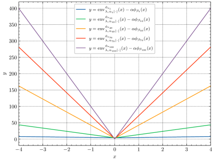
Figure B.1: Plots of $y=\mathrm{env}_{\lambda,\alpha_{i}|\cdot|}^{\psi_{\sigma_{i}}}(x)-\alpha\phi_{\beta_{i}}(x)$, for $i\in\{1,10,40,70,100\}$.

Figure B.1 shows that the above choices give a convex $\overleftarrow{\mathrm{env}}_{\lambda,g}^{\psi_{\bm{\sigma}}}-\alpha\varphi_{\bm{\beta}}$.

Similarly, we also show graphically that $\beta_{g}\varphi_{\bm{\beta}}-\overleftarrow{\mathrm{env}}_{\lambda,g}^{\psi_{\bm{\sigma}}}$ is convex for some $\beta_{g}>0$, e.g., $\beta_{g}=2500$ (not tight).

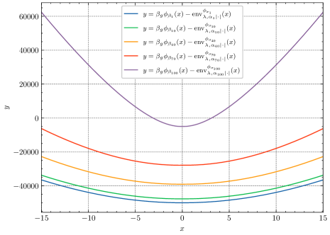
Figure B.2: Plots of $y=\beta_{g}\phi_{\beta_{i}}(x)-\mathrm{env}_{\lambda,\alpha_{i}|\cdot|}^{\psi_{\sigma_{i}}}(x)$, for $i\in\{1,10,40,70,100\}$.

Since all Assumptions 3.1, 3.2, 3.3, 3.4, 3.5 and 3.8 are satisfied, $g$ is Lipschitz and $\psi$ is strongly convex, the convergence results in the main text, i.e., Theorem 4.2 and Corollary 4.3, hold.

Appendix C The Bregman–Moreau Mirrorless Mirror-Langevin Algorithm

In this section, we give the details of the Bregman–Moreau mirrorless mirror-Langevin algorithm (BMMMLA), whose results are mostly taken from Ahn and Chewi (2021).

C.1 Assumptions

We first state the assumptions required in Ahn and Chewi (2021). Instead of the modified self-concordance condition, the Legenedre function $\varphi$ has to be $M_{\varphi}$-self-concordant (Nesterov, 2018, §5.1.3), i.e., for any $x\in\mathcal{X}$, there exists $M_{\varphi}\geqslant 0$ such that $\left|\nabla^{3}\varphi(x)[u,u,u]\right|\leqslant 2M_{\varphi}\|u\|_{\nabla^{2}\varphi(x)}^{3}$ for all $u\in\mathbb{R}^{d}$. Furthermore, in addition to the $\alpha$-relative convexity (to $\varphi$) and $\beta$-relative smoothness (to $\varphi$) assumption, $U_{\lambda}^{\psi}$ also has to be $L$-Lipschitz relative to $\varphi$, which is defined as follows.

Definition C.1 (Relative Lipschitz continuity).

A function $f\in\mathscr{C}^{1}$ is $L$-Lipschitz relative to a very strictly convex (see Assumption 3.3(iii)) Legendre function $\varphi$ if there exists $L>0$ such that $\|\nabla f(x)\|_{[\nabla^{2}\varphi(x)]^{-1}}\leqslant L$ for all $x\in\operatorname*{int}\operatorname*{dom}f$.

It is worth noting that it is difficult to verify that Bregman–Moreau envelopes would satisfy such a relative Lipschitzness condition in general.

Now we let $x_{0}\in\mathcal{Y}$. Similar to MLA (7) in Ahn and Chewi (2021), the Bregman–Moreau mirrorless Mirror-Langevin algorithm (BMMMLA) iterates

$$x_{k+\nicefrac{{1}}{{2}}} =\nabla\varphi^{*}\left(\nabla\varphi(x_{k})-\gamma\nabla U_{\lambda}^{\psi}(x_{k})\right),$$

$$x_{k+1} =\nabla\varphi^{*}(Y_{\gamma}),$$

where

$$\begin{cases}\mathrm{d}Y_{t}=\sqrt{2}\left[\nabla^{2}\varphi^{*}(Y_{t})\right]^{-\nicefrac{{1}}{{2}}}\,\mathrm{d}W_{t}\\ Y_{0}=\nabla\varphi\left(x_{k+\nicefrac{{1}}{{2}}}\right)=\nabla\varphi(x_{k})-\gamma\nabla U_{\lambda}^{\psi}(x_{k}).\end{cases}$$ (C.1)

C.2 Convergence Results

We suppose that the assumptions in Section C.1 hold. We define the mixture distribution $\overline{\mu}_{K}\coloneqq\frac{1}{K}\sum_{k=1}^{K}\mu_{k}$, and let $\beta^{\prime}\coloneqq\beta+2M_{\varphi}L$. Then we have the following convergence results.

Theorem C.2 (Convex).

Assume $\alpha=0$ and $\beta^{\prime}>0$. Let $X_{k}\sim\mu_{k}$ be generated by (C.1) with step size $\gamma=\min\left\{\varepsilon/(2\beta^{\prime}d),1/\beta^{\prime}\right\}$. Then for all $\varepsilon>0$, there exists $\lambda>0$ such that $D_{\mathrm{KL}}(\overline{\mu}_{K}\,|\kern-1.07639pt|\,\pi_{\lambda}^{\psi})\leqslant\varepsilon$ for

$$K\geqslant\frac{4d\beta^{\prime}\mathsf{D}_{\varphi}(\pi,\mu_{0})}{\varepsilon^{2}}\max\left\{1,\frac{\varepsilon}{2d}\right\}.$$

Theorem C.3 (Legendre strongly convex).

Assume $\alpha>0$ and $\beta^{\prime}>0$. Suppose that $X_{0}\sim\mu_{0}$ satisfies $\mathsf{D}_{\varphi}(\pi,\mu_{0})\leqslant\varepsilon$. Let $X_{k}\sim\mu_{k}$ be generated by (C.1) with step size $\gamma=\min\left\{\varepsilon/(2\beta^{\prime}d),1/\beta^{\prime}\right\}$. Then for all $\varepsilon>0$, there exists $\lambda>0$ such that $D_{\mathrm{KL}}(\overline{\mu}_{K}\,|\kern-1.07639pt|\,\pi_{\lambda}^{\psi})\leqslant\varepsilon$ for

$$K\geqslant\frac{4\beta^{\prime}d}{\varepsilon}\max\left\{1,\frac{\varepsilon}{2d}\right\}.$$

The results follow from Ahn and Chewi (2021, Theorems 1 and 2(b)). Similar bounds on the total variation distance follows from Pinsker’s inequality: $\|P-Q\|_{\mathrm{TV}}^{2}\leqslant\frac{1}{2}D_{\mathrm{KL}}(P\,|\kern-1.07639pt|\,Q)$, and also bounds on the total variation distance between $\overline{\mu}_{K}$ and the target distribution $\pi$ instead of the surrogate distribution $\pi_{\lambda}^{\psi}$. $\Box$

Note also that convergence in the Bregman transport cost also holds (Ahn and Chewi, 2021, Theorem 2(a)), where the Bregman transport cost is defined as follows.

Definition C.4 (Bregman transport cost).

For two probability measures $\mu$ and $\nu$ on $\mathcal{B}(\mathbb{R}^{d})$, the Bregman transport cost (Cordero-Erausquin, 2017) from $\mu$ to $\nu$ with respect to the Bregman divergence associated with a Legendre function $\varphi$ is defined by

$$\mathsf{D}_{\varphi}(\mu,\nu)\coloneqq\inf_{\pi\sim\Pi(\mu,\nu)}\int_{\mathbb{R}^{d}\times\mathbb{R}^{d}}D_{\varphi}(x,y)\,\mathrm{d}\pi(x,y).$$

We also refer to Ahn and Chewi (2021, Theorem 2.1) for convergence results in terms of the Bregman transport cost (Cordero-Erausquin, 2017). By Pinsker’s inequality, we can also obtain similar results in terms of the total variation distance.

Finally, we give the Bregman–Moreau mirrorless mirror-Langevin algorithm (C.1) with an Euler–Maruyama discretization for the second step.

Algorithm 1 The Bregman–Moreau Mirrorless Mirror-Langevin Algorithm (BMMMLA)

  Initialize: Legendre functions $\varphi$ and $\psi$, $\bm{\theta}_{0}\in\mathbb{R}^{d}$, step size $\gamma\in\left]0,+\infty\right[$, number of samples to be drawn $K\in\mathbb{N}^{*}$, number of inner steps of Euler–Maruyama discretization $N\in\mathbb{N}^{*}$.

  for $k=0,1,2,\ldots,K-1$ do

     $\bm{\theta}_{k+\nicefrac{{1}}{{2}}}=\nabla\varphi^{*}\left(\nabla\varphi(\bm{\theta}_{k})-\gamma\nabla U_{\lambda}^{\psi}(\bm{\theta}_{k})\right)$

     $\bm{y}_{0}=\nabla\varphi\left(\bm{\theta}_{k+\nicefrac{{1}}{{2}}}\right)=\nabla\varphi(\bm{\theta}_{k})-\gamma\nabla U_{\lambda}^{\psi}(\bm{\theta}_{k})$

     for $n=0,1,2,\ldots,N$ do

        $\bm{\xi}_{n}\sim\mathsf{N}_{d}(\bm{0}_{d},I_{d})$

        $\bm{y}_{n+1}=\bm{y}_{n}+\sqrt{2\gamma/N}\left[\nabla^{2}\varphi^{*}(\bm{y}_{n})\right]^{-\nicefrac{{1}}{{2}}}\bm{\xi}_{n}$

     end for

     $\bm{\theta}_{k+1}=\nabla\varphi^{*}(\bm{y}_{N+1})$

  end for

We also give the experimental results of the Bregman–Moreau mirrorless mirror-Langevin algorithm in Appendix D.

Appendix D Additional Numerical Experiments

D.1 Anisotropic Laplace Distribution

We first give more plots of different dimensions for the experiment in Section 5.

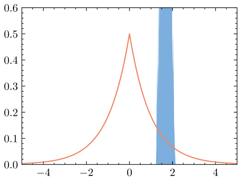
(a) 1^st dimension

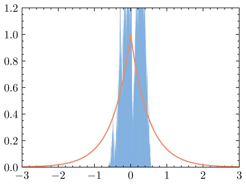
(b) 2^nd dimension

(c) 5^th dimension

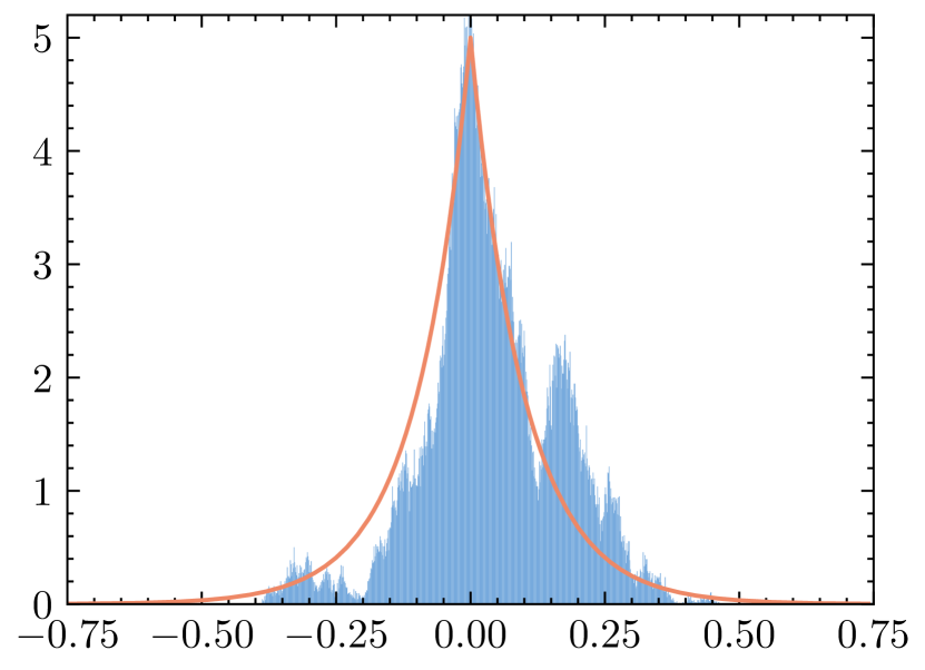
(d) 10^th dimension

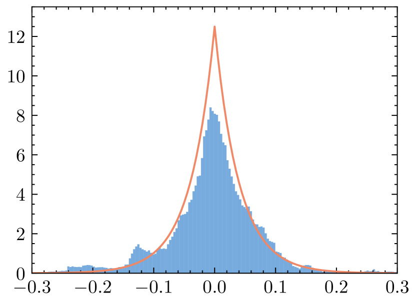
(e) 25^th dimension

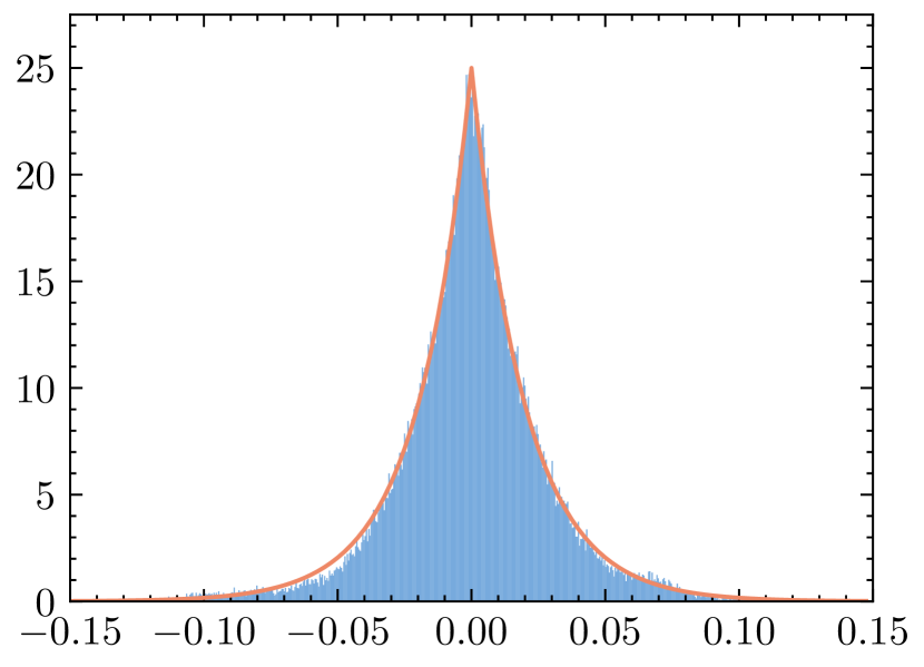
(f) 50^th dimension

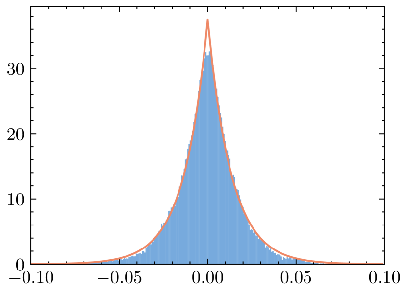
(g) 75^th dimension

(h) 100^th dimension

Figure D.1: Histograms of samples (blue) from MYULA and the true densities (orange).

(a) 1^st dimension

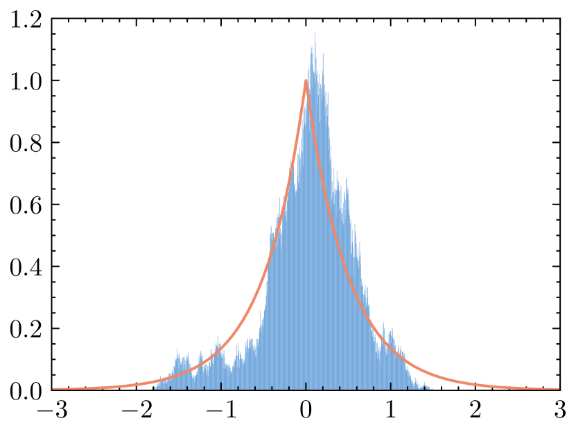
(b) 2^nd dimension

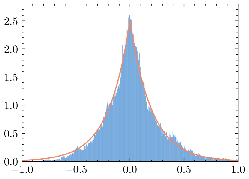
(c) 5^th dimension

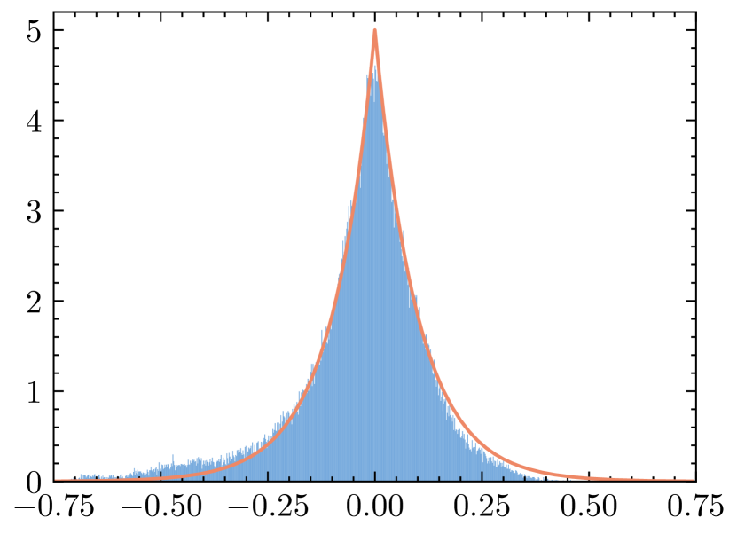
(d) 10^th dimension

(e) 25^th dimension

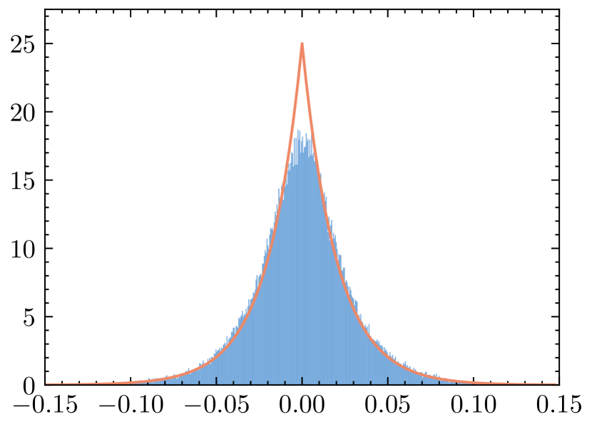
(f) 50^th dimension

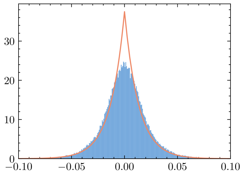
(g) 75^th dimension

(h) 100^th dimension

Figure D.2: Histograms of samples (blue) from BMUMLA and the true densities (orange).

We also give the experimental results using a different (left) Bregman–Moreau envelope introduced in Section B.1, using the same step size $\gamma=5\times 10^{-6}$ in Figure D.3.

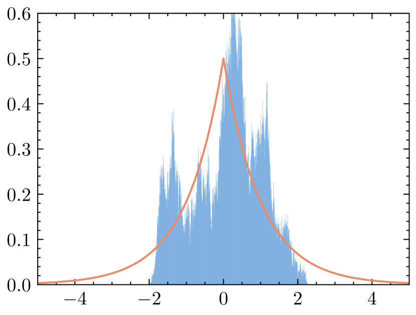
(a) 1^st dimension

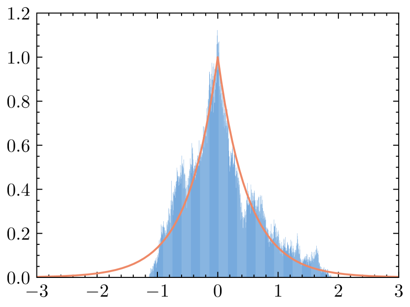
(b) 2^nd dimension

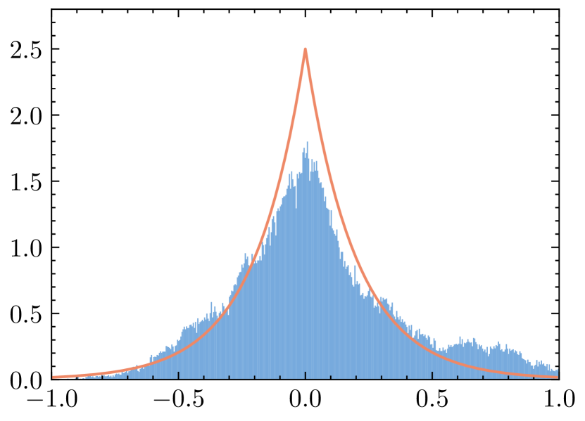
(c) 5^th dimension

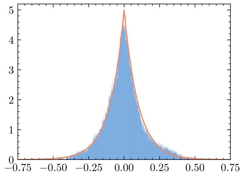
(d) 10^th dimension

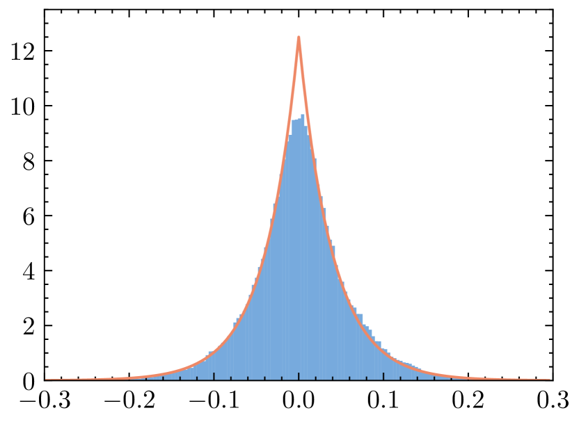
(e) 25^th dimension

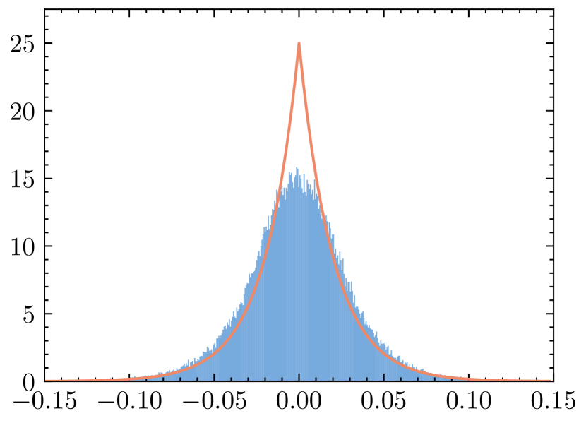
(f) 50^th dimension

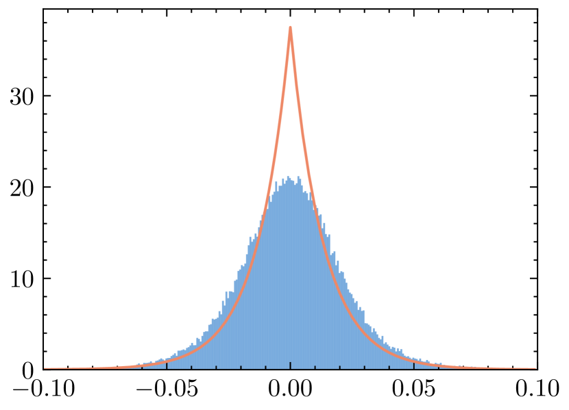
(g) 75^th dimension

(h) 100^th dimension

Figure D.3: Histograms of samples (blue) from LBMUMLA and the true densities (orange) with a different Bregman–Moreau envelope.

On the other hand, for practical purpose, we also perform the same set of experiments with another Bregman–Moreau envelope associated to the Legendre function $\psi(\bm{\theta})=\sum_{i=1}^{d}\mathrm{e}^{\theta_{i}}$. This is chosen particularly because we can compute the corresponding closed form expressions of both of its associated left and right Bregman proximity operators. To do so, we compute the following left and right Bregman proximity operators associated to the exponential function.

Proposition D.1.

The left Bregman proximity operator of $\alpha|\cdot|$ associated to the Legendre function $\exp$ for $\alpha>0$ is

$$\overleftarrow{\operatorname{P}}_{\negthinspace\negthinspace\lambda,\alpha|\cdot|}^{\exp}(\theta)=\begin{cases*}\log(\mathrm{e}^{\theta}-\alpha\lambda)&if $\theta>\log(1+\alpha\lambda)$,\\ \log(\mathrm{e}^{\theta}+\alpha\lambda)&if $\theta<\log(1-\alpha\lambda)$,\\ 1-\mathrm{e}^{\theta}(1+\theta)&otherwise.\end{cases*}$$

The right Bregman proximity operator of $\alpha|\cdot|$ associated to the Legendre function $\exp$ for $\alpha>0$ is

$$\overrightarrow{\operatorname{P}}_{\negthinspace\negthinspace\lambda,\alpha|\cdot|}^{\exp}(\theta)=\begin{cases*}W(-\alpha\lambda\mathrm{e}^{-\theta})+\theta&if $\theta>\alpha\lambda$,\\ W(\alpha\lambda\mathrm{e}^{-\theta})+\theta&if $\theta<-\alpha\lambda$,\\ \mathrm{e}^{\theta}-(1+\theta)&otherwise,\end{cases*}$$

where $W$ is the Lambert $W$ function (Lambert, 1758; Corless et al., 1996), i.e., the inverse of $\xi\mapsto\xi\mathrm{e}^{\xi}$ on $\left[0,+\infty\right[$.

Proof of Proposition D.1.

According to Definition 2.5,

$$\overleftarrow{\operatorname{P}}_{\negthinspace\negthinspace\lambda,\alpha|\cdot|}^{\exp}(\theta)=\operatorname*{argmin}_{\vartheta\in\mathbb{R}}\,\left\{\lambda\alpha|\vartheta|+\mathrm{e}^{\vartheta}-\mathrm{e}^{\theta}-\mathrm{e}^{\theta}(\vartheta-\theta)\right\}.$$

First-order conditions give

$$\begin{cases*}\alpha\lambda+\mathrm{e}^{\vartheta}-\mathrm{e}^{\theta}=0&if $\vartheta>0$,\\ -\alpha\lambda+\mathrm{e}^{\vartheta}-\mathrm{e}^{\theta}=0&if $\vartheta<0$,\end{cases*}$$

which implies

$$\vartheta^{\star}=\begin{cases*}\log(\mathrm{e}^{\theta}-\alpha\lambda)&if $\vartheta^{\star}>0$,\\ \log(\mathrm{e}^{\theta}+\alpha\lambda)&if $\vartheta^{\star}<0$\end{cases*}=\begin{cases*}\log(\mathrm{e}^{\theta}-\alpha\lambda)&if $\theta>\log(1+\alpha\lambda)$,\\ \log(\mathrm{e}^{\theta}+\alpha\lambda)&if $\theta<\log(1-\alpha\lambda)$.\end{cases*}$$ (D.1)

On the other hand, if $\vartheta=0$, then

$$\operatorname*{argmin}_{\vartheta\in\mathbb{R}}\,\left\{\lambda\alpha|\vartheta|+\mathrm{e}^{\vartheta}-\mathrm{e}^{\theta}-\mathrm{e}^{\theta}(\vartheta-\theta)\right\}=\operatorname*{argmin}_{\vartheta\in\mathbb{R}}\,\left\{1-\mathrm{e}^{\theta}+\theta\mathrm{e}^{\theta}\right\}=1-\mathrm{e}^{\theta}(1+\theta),$$ (D.2)

which corresponds to the range $[\log(1-\alpha\lambda),\log(1+\alpha\lambda)]$ for $\theta$. Combining (D.1) and (D.2) yields the first desired result.

Again, according to Definition 2.5,

$$\overrightarrow{\operatorname{P}}_{\negthinspace\negthinspace\lambda,\alpha|\cdot|}^{\exp}(\theta)=\operatorname*{argmin}_{\vartheta\in\mathbb{R}}\,\left\{\lambda\alpha|\vartheta|+\mathrm{e}^{\theta}-\mathrm{e}^{\vartheta}-\mathrm{e}^{\vartheta}(\theta-\vartheta)\right\}.$$

First-order conditions give

$$\begin{cases*}\alpha\lambda-\mathrm{e}^{\vartheta}(\theta-\vartheta)=0&if $\vartheta>0$,\\ -\alpha\lambda-\mathrm{e}^{\vartheta}(\theta-\vartheta)=0&if $\vartheta<0$\end{cases*}\Leftrightarrow\begin{cases*}(\vartheta-\theta)\mathrm{e}^{\vartheta-\theta}=-\alpha\lambda\mathrm{e}^{-\theta}&if $\vartheta>0$,\\ (\vartheta-\theta)\mathrm{e}^{\vartheta-\theta}=\alpha\lambda\mathrm{e}^{-\theta}&if $\vartheta<0$,\end{cases*}$$

which implies

$$\vartheta^{\star} =\begin{cases*}W(-\alpha\lambda\mathrm{e}^{-\theta})+\theta&if $\vartheta^{\star}>0$ and $-\alpha\lambda\mathrm{e}^{-\theta}\geqslant-\mathrm{e}^{-1}$,\\ W(\alpha\lambda\mathrm{e}^{-\theta})+\theta&if $\vartheta^{\star}<0$\end{cases*}$$

$$=\begin{cases*}W(-\alpha\lambda\mathrm{e}^{-\theta})+\theta&if $\theta>\alpha\lambda$ and $\theta\geqslant\log(\alpha\lambda)+1$,\\ W(\alpha\lambda\mathrm{e}^{-\theta})+\theta&if $\theta<-\alpha\lambda$.\end{cases*}$$

$$=\begin{cases*}W(-\alpha\lambda\mathrm{e}^{-\theta})+\theta&if $\theta>\alpha\lambda$,\\ W(\alpha\lambda\mathrm{e}^{-\theta})+\theta&if $\theta<-\alpha\lambda$.\end{cases*}$$ (D.3)

since $u\geqslant\log u+1$ for any $u>0$. Notice that the condition $-\alpha\lambda\mathrm{e}^{-\theta}\geqslant-\mathrm{e}^{-1}$ is required for the Lambert $W$ function to be defined for a negative value.

On the other hand, if $\vartheta=0$, then

$$\operatorname*{argmin}_{\vartheta\in\mathbb{R}}\,\left\{\lambda\alpha|\vartheta|+\mathrm{e}^{\theta}-\mathrm{e}^{\vartheta}-\mathrm{e}^{\vartheta}(\theta-\vartheta)\right\}=\operatorname*{argmin}_{\vartheta\in\mathbb{R}}\,\left\{\mathrm{e}^{\theta}-1-\theta\right\}=\mathrm{e}^{\theta}-(1+\theta),$$ (D.4)

which corresponds to the range $[-\alpha\lambda,\alpha\lambda]$ for $\theta$. Combining (D.1) and (D.4) yields the second desired result. ∎

The corresponding experiments are illustrated in Figure D.4. BMMMLA (Figure D.5) are also used in this setting. We observe that the right variants perform comparably to the left ones, both outperforming MYULA at the wide marginals (i.e., the lower dimensions).

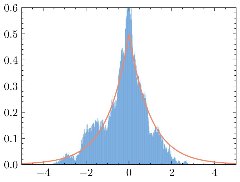
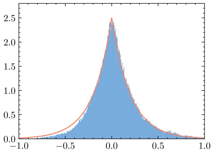
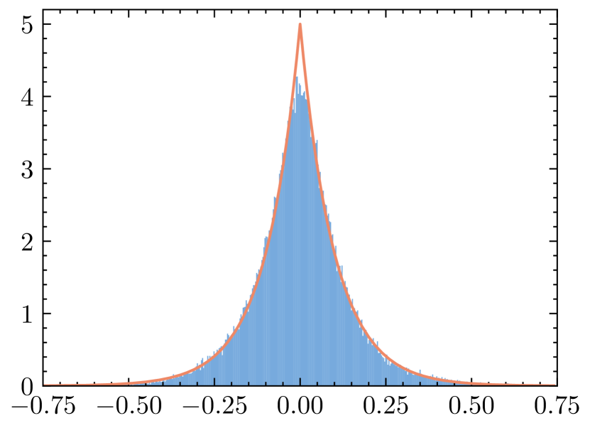
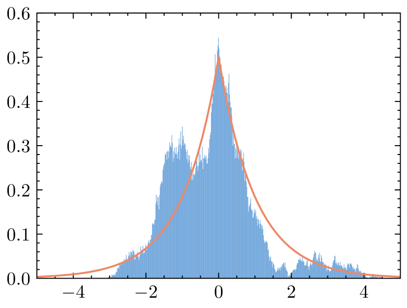
(a) 1^st dimension

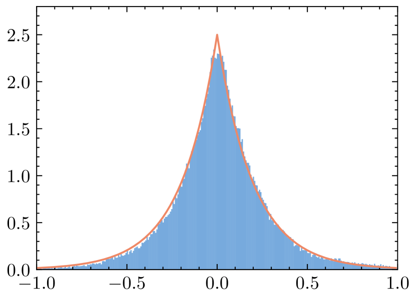
(b) 5^th dimension

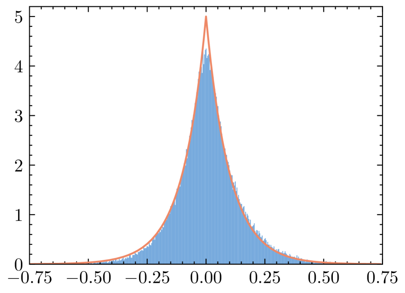
(c) 10^th dimension

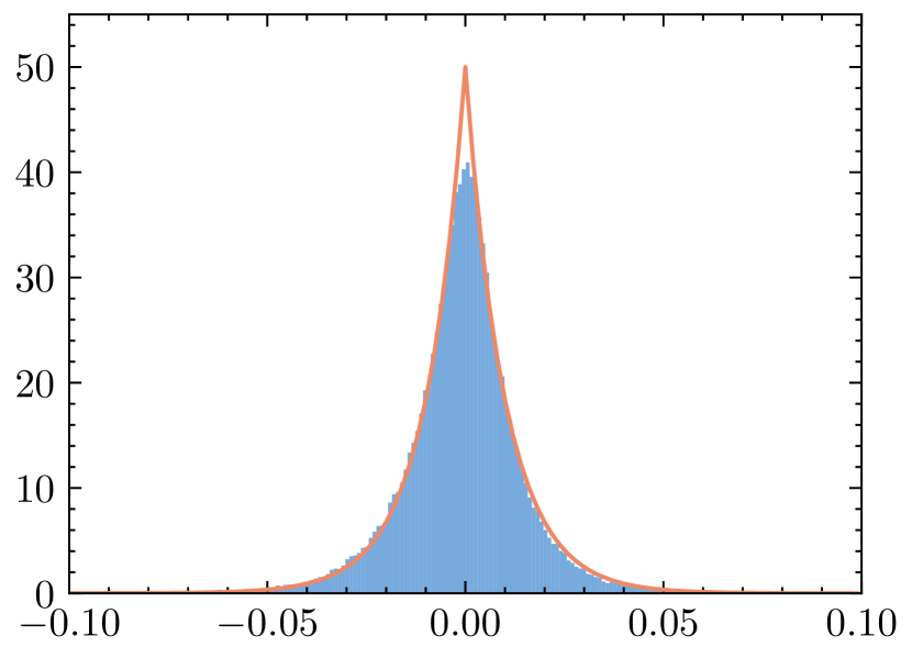
(d) 100^th dimension

Figure D.4: Histograms of samples (in blue) from left BMUMLA (1^st row), right BMUMLA (2^nd row) and the true densities (in orange).

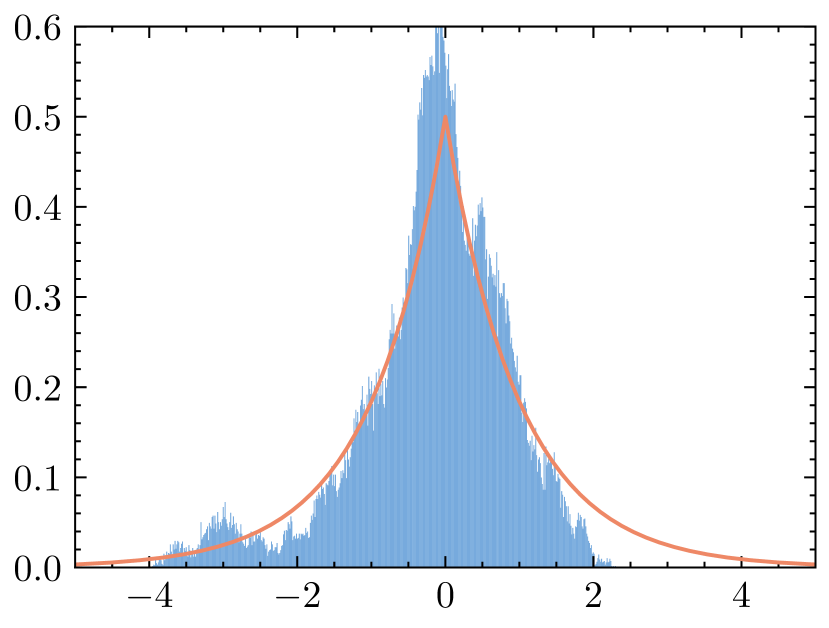
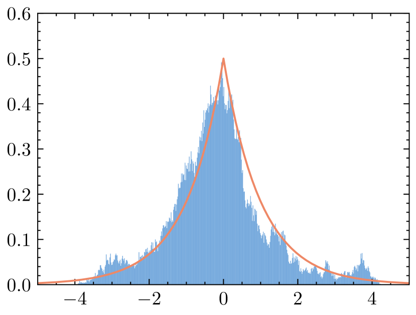
(a) 1^st dimension

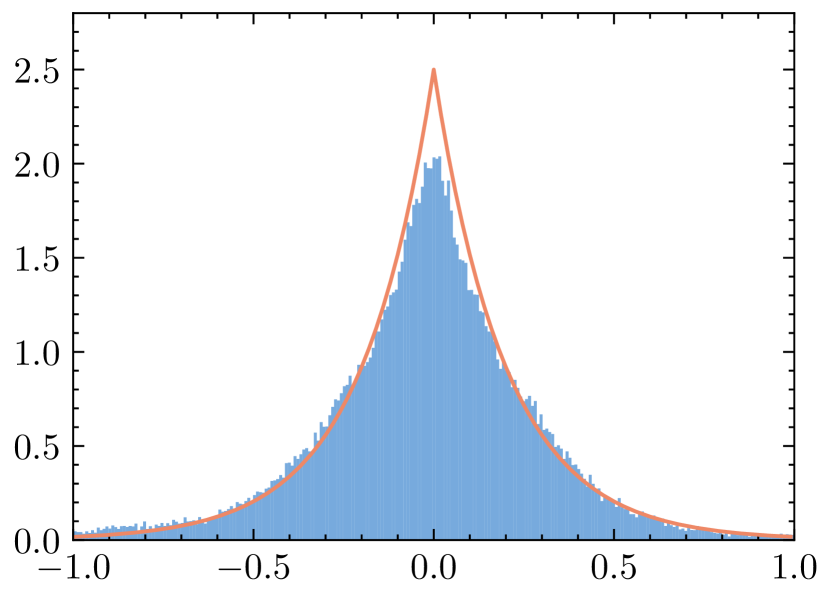
(b) 5^th dimension

(c) 10^th dimension

(d) 100^th dimension

Figure D.5: Histograms of samples (in blue) from left BMMMLA (1^st row), right BMMMLA (2^nd row) and the true densities (in orange).

D.2 Anisotropic Uniform Distribution

We consider the task of sampling from an anisotropic uniform distribution over the set $\mathcal{C}\coloneqq\prod_{i=1}^{d}[a_{i},b_{i}]$, where $\bm{a}=(a_{i})_{1\leqslant i\leqslant d}^{\top}\in\mathbb{R}^{d}$ and $\bm{b}=(b_{i})_{1\leqslant i\leqslant d}^{\top}\in\mathbb{R}^{d}$. To perform this task using our proposed algorithm, we let $f=0$ and $g=\iota_{\mathcal{C}}$. Note that the original mirror Langevin algorithm cannot apply to sampling uniform distributions, as mentioned in Li et al. (2022), as $f=0$. However, by suitably choosing a Bregman–Moreau envelope, we can still perform approximate sampling (as opposed to exact sampling) using the BMMMLA.

Note that when $g=\iota_{\mathcal{C}}$ with $\mathcal{C}\subseteq\mathbb{R}^{d}$ being a closed convex set, the Bregman proximity operators of $g$ are the Bregman projections (or projectors) onto $\mathcal{C}$, as illustrated in the following definition (Bauschke et al., 2018).

Definition D.2 (Bregman projections).

Let $\mathcal{C}\subseteq\mathbb{R}^{d}$ be a closed convex set such that $\mathcal{X}\cap\mathcal{C}\neq\varnothing$, then $\overleftarrow{\operatorname{P}}_{\negthinspace\negthinspace\mathcal{C}}^{\varphi}\coloneqq\overleftarrow{\operatorname{P}}_{\negthinspace\negthinspace\iota_{\mathcal{C}}}^{\varphi}$ and $\overrightarrow{\operatorname{P}}_{\negthinspace\negthinspace\mathcal{C}}^{\varphi}\coloneqq\overrightarrow{\operatorname{P}}_{\negthinspace\negthinspace\iota_{\mathcal{C}}}^{\varphi}$ are the left and right Bregman projections onto $\mathcal{C}$ respectively.

For simplicity, we choose $\psi=\frac{1}{2}\left\lVert\cdot\right\rVert_{2}^{2}$. Then the Bregman projection onto $\mathcal{C}$ boils down to the Euclidean projection onto $\mathcal{C}$, which is given by

$$\overleftarrow{\operatorname{P}}_{\negthinspace\negthinspace\mathcal{C}}^{\varphi}(\bm{\theta})=\overrightarrow{\operatorname{P}}_{\negthinspace\negthinspace\mathcal{C}}^{\varphi}(\bm{\theta})=\operatorname{proj}_{\mathcal{C}}(\bm{\theta})=\left(\min\{b_{i},\max\{a_{i},\theta_{i}\}\}\right)_{1\leqslant i\leqslant d}^{\top}.$$

In the experiment, we consider the case where $a_{i}=-i$ and $b_{i}=i$ for all $i\in\llbracket d\rrbracket$, so that the target uniform distribution on $\mathcal{C}=[-1,1]\times[-2,2]\times\cdots\times[-d,d]$ is anisotropic, varying significantly across different dimensions. We use $\gamma=0.01$, $\lambda=1$ and $\bm{\beta}=(2\sqrt{d-i+1})_{1\leqslant i\leqslant d}^{\top}$, and give the experimental results in Figures D.6 and D.7. We observe that BMUMLA outperforms MYULA at higher dimensions with wide marginals, where most samples lie in the desired ranges. Also note that all of Assumptions 3.1, 3.2, 3.3, 3.4, 3.5 and 3.8 hold. See Figure D.8 as a graphical verification of Assumption 3.8, with $\alpha=2M_{\varphi_{\bm{\beta}}}+0.1$ and $\beta_{g}=250$.

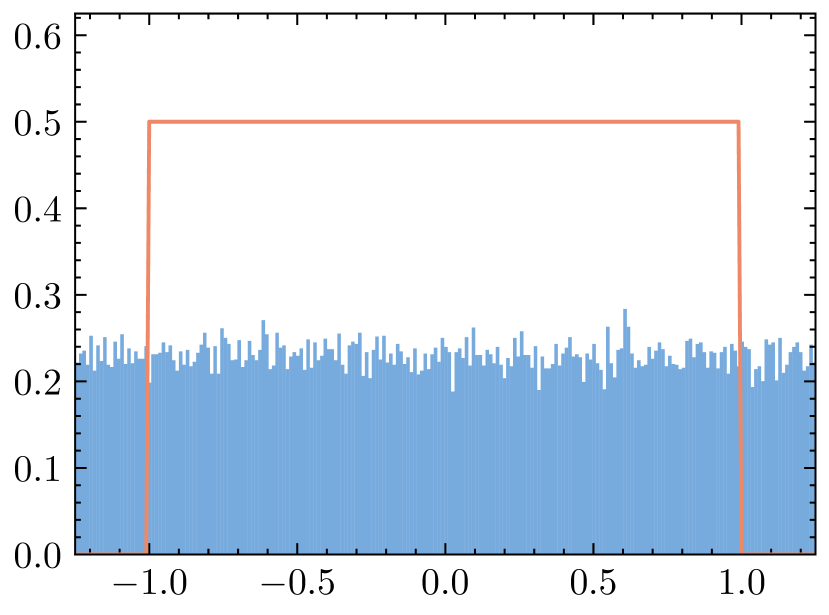
(a) 1^st dimension

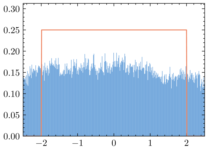
(b) 2^nd dimension

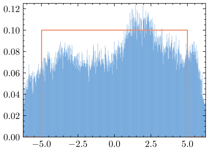
(c) 5^th dimension

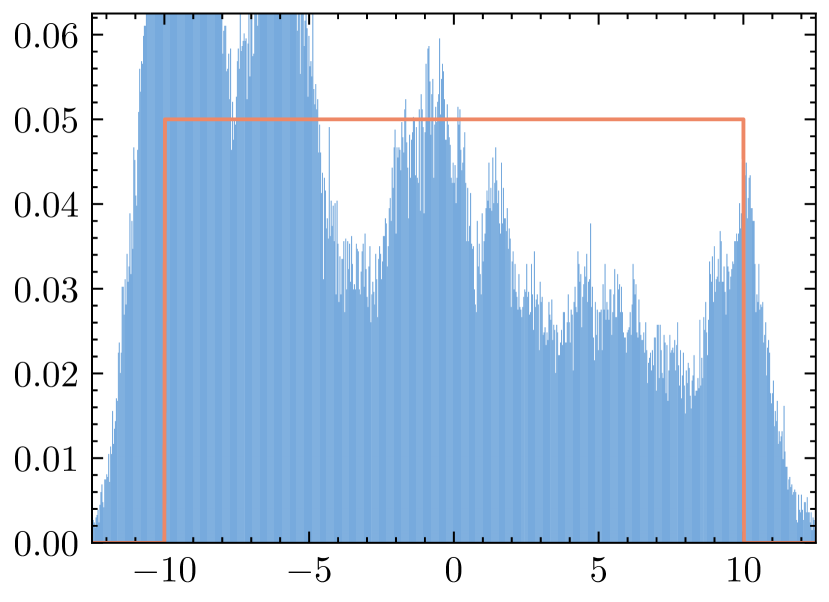
(d) 10^th dimension

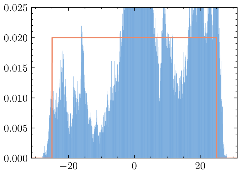
(e) 25^th dimension

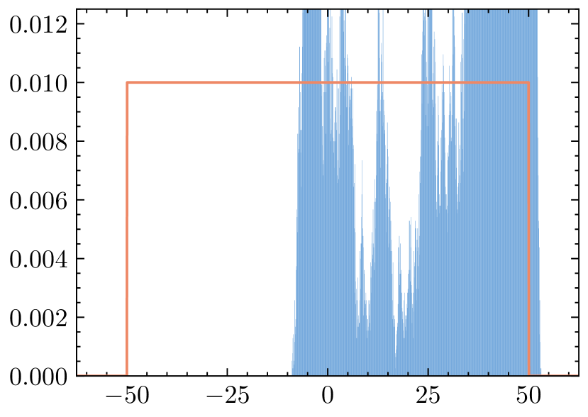
(f) 50^th dimension

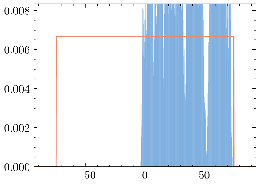
(g) 75^th dimension

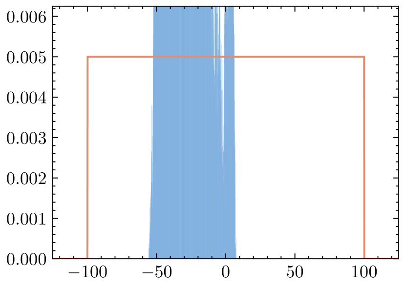
(h) 100^th dimension

Figure D.6: Histograms of samples (blue) from MYULA and the true densities (orange) for uniform distribution on $\mathcal{C}$.

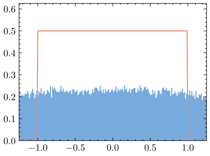
(a) 1^st dimension

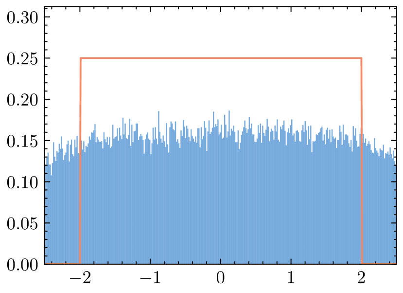
(b) 2^nd dimension

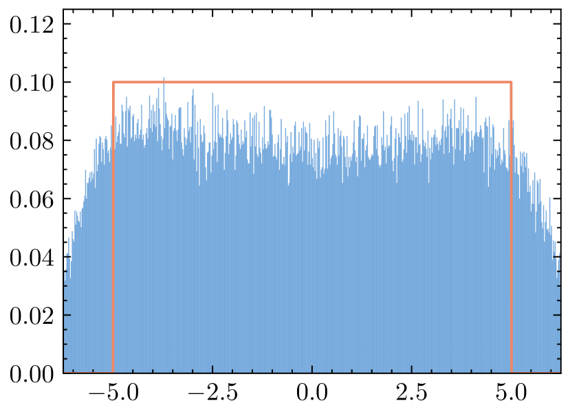
(c) 5^th dimension

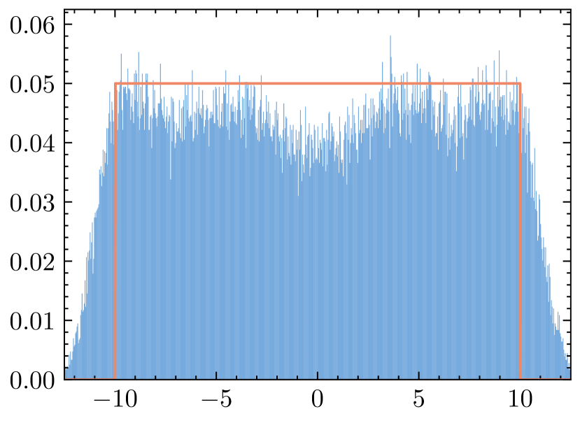
(d) 10^th dimension

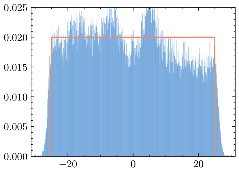
(e) 25^th dimension

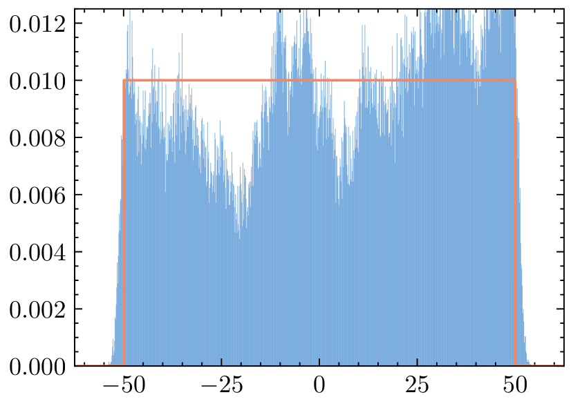
(f) 50^th dimension

(g) 75^th dimension

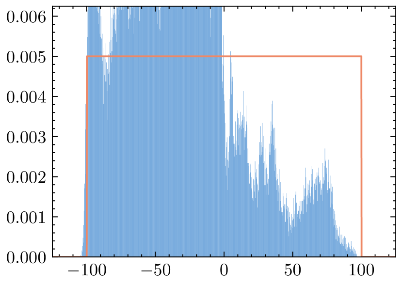
(h) 100^th dimension

Figure D.7: Histograms of samples (blue) from BMUMLA and the true densities (orange) for uniform distribution on $\mathcal{C}$.

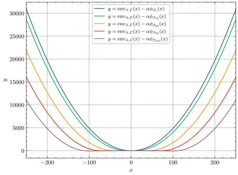
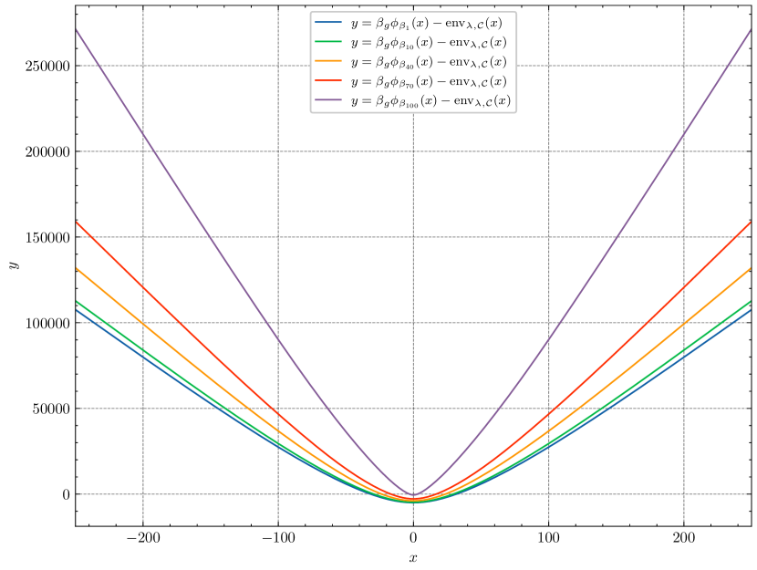
Figure D.8: Plots of $y=\mathrm{env}_{\lambda,\mathcal{C}}(x)-\alpha\phi_{\beta_{i}}(x)$ (left) and $y=\beta_{g}\phi_{\beta_{i}}(x)-\mathrm{env}_{\lambda,\mathcal{C}}(x)$ (right), for $i\in\{1,10,40,70,100\}$.

D.3 Bayesian Sparse Logistic Regression

We compare the performance of MYULA and BMUMLA in Bayesian sparse logistic regression. Suppose that we observe the samples $\{(\bm{x}_{n},y_{n})\}_{n=1}^{N}$, where $\bm{x}_{n}\in\mathbb{R}^{d}$ and $y_{n}\in\{0,1\}$. In Bayesian logistic regression, the data are assumed to follow the model

$$y_{n}\stackrel{{\scriptstyle\text{i.i.d.}}}{{\sim}}\mathrm{Bernoulli}\left(\frac{\exp(\left\langle\bm{\theta},\bm{x}_{n}\right\rangle)}{1+\exp(\left\langle\bm{\theta},\bm{x}_{n}\right\rangle)}\right),$$ (D.5)

for each $n\in\llbracket N\rrbracket$. The parameter $\bm{\theta}=(\theta_{i})_{1\leqslant i\leqslant d}^{\top}\in\mathbb{R}^{d}$ is a random variable with a prior density $p$ with respect to Lebesgue measure. Then, the posterior distribution of $\bm{\theta}$ takes the form

$$p(\bm{\theta}\,|\,\{(\bm{x}_{n},y_{n})\}_{n=1}^{N})\propto p(\bm{\theta})\exp\left\{\sum_{n=1}^{N}\left(y_{n}\left\langle\bm{\theta},\bm{x}_{n}\right\rangle-\log(1+\exp(\left\langle\bm{\theta},\bm{x}_{n}\right\rangle))\right)\right\}.$$

We are particularly concerned with the case with a prior in the form of a combination of an anisotropic Laplace distribution (which is sparsity-inducing) and a Gaussian distribution, where the unadjusted Langevin algorithm is no longer viable due to the nonsmoothness induced by the anisotropic Laplace distribution. In general, such a prior takes the form:

$$p(\bm{\theta})\coloneqq p(\bm{\theta}\,|\,\bm{\alpha}_{1},\alpha_{2})\propto\exp\left\{-\sum_{i=1}^{d}\alpha_{1,i}|\theta_{i}|-\frac{\alpha_{2}}{2}\sum_{i=1}^{d}\theta_{i}^{2}\right\},$$

where $\bm{\alpha}_{1}=(\alpha_{1,i})_{1\leqslant i\leqslant d}^{\top}\in\left[0,+\infty\right[^{d}$ and $\alpha_{2}\in\left[0,+\infty\right[$.

Then, the resulting posterior distribution has a potential of the following form:

$$U(\bm{\theta})=\underbrace{\sum_{n=1}^{N}[\log(1+\exp(\left\langle\bm{\theta},\bm{x}_{n}\right\rangle))-y_{n}\left\langle\bm{\theta},\bm{x}_{n}\right\rangle]+\alpha_{2}\left\lVert\bm{\theta}\right\rVert_{2}^{2}}_{\eqqcolon f(\bm{\theta})}+\underbrace{\left\|\bm{\alpha}_{1}\odot\bm{\theta}\right\|_{{1}}}_{\eqqcolon g(\bm{\theta})}.$$

We take $d=100$, $N=1000$ and $\bm{\theta}^{\star}=(\bm{0}_{10}^{\top},0.1\cdot\bm{1}_{10}^{\top},0.2\cdot\bm{1}_{10}^{\top},\ldots,0.9\cdot\bm{1}_{10}^{\top})^{\top}\in\mathbb{R}^{100}$ as the ground truth. Then, each $x_{n,i}$ is generated from a standard Gaussian distribution and each $y_{n}$ is sampled following (D.5) with $\bm{\theta}=\bm{\theta}^{\star}$. In addition, we choose $\bm{\alpha}_{1}=(10\cdot\bm{1}_{10}^{\top},9\cdot\bm{1}_{10}^{\top},\ldots,1\cdot\bm{1}_{10}^{\top})^{\top}$ and $\alpha_{2}=0.1$. Again, we use the hypentropy functions $\varphi_{\bm{\beta}}$ (for the mirror map) and $\psi_{\bm{\sigma}}$ (for the Bregman–Moreau envelope), with $\bm{\beta}=(2i^{\nicefrac{{1}}{{4}}}\cdot\bm{1}_{10}^{\top})_{1\leqslant i\leqslant 10}^{\top}$ and $\bm{\sigma}=(\alpha_{1,i}^{2})_{1\leqslant i\leqslant d}^{\top}$. We also use a step size $\gamma=5\times 10^{-4}$ and a smoothing parameter $\lambda=0.01$. Note that all of Assumptions 3.1, 3.2, 3.3, 3.4, 3.5 and 3.8 hold in this case. In particular, for Assumption 3.8, notice that $f$ is indeed strongly convex.

We compare the performance of MYULA and BMUMLA by estimating the posterior means of $\bm{\theta}$ (as a whole or componentwise) and $\left\lVert\bm{\theta}\right\rVert_{2}^{2}/d$. We generate 30 samples (indexed by $s$) using each algorithm for 4000 iterations and average the samples to obtain estimates $\bm{\theta}_{k}=\frac{1}{30}\sum_{s=1}^{30}\bm{\theta}_{k,s}$ and $\left\lVert\bm{\theta}_{k}\right\rVert_{2}^{2}/d$ for the posterior means. From Figure D.9, we observe that the proposed left BMUMLA outperforms MYULA in the estimation of both posterior means.

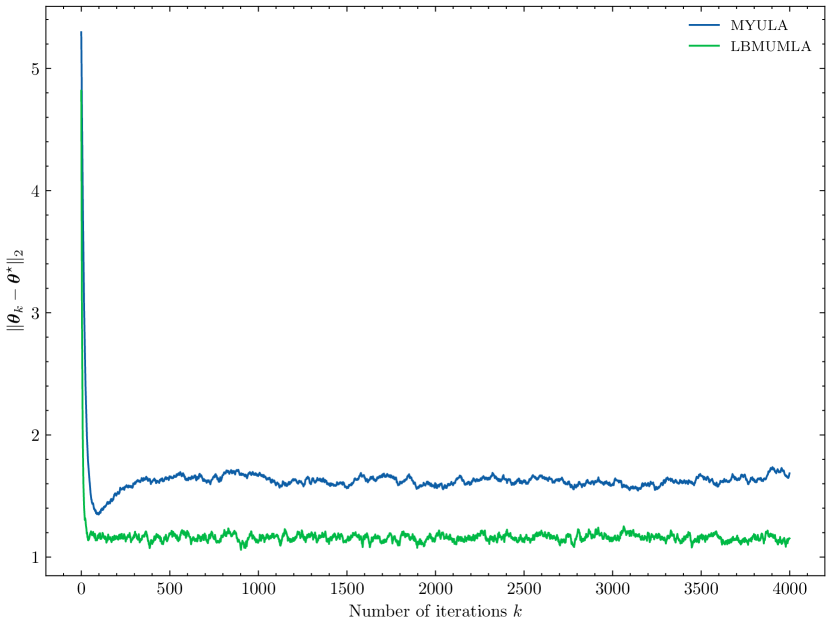
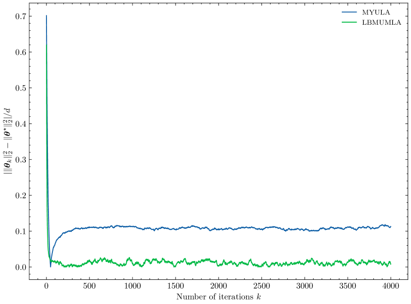
Figure D.9: Plots of estimation errors of the posterior means $\left\lVert\bm{\theta}_{k}-\bm{\theta}^{\star}\right\rVert_{2}$ (left) and $\left|\left\lVert\bm{\theta}_{k}\right\rVert_{2}^{2}-\left\lVert\bm{\theta}^{\star}\right\rVert_{2}^{2}\right|/d$ (right).

We also plot the estimation errors of the posterior means of some components of $\bm{\theta}$. Figure D.10 reveals that MYULA gives smaller estimation errors than LBMUMLA at lower dimensions but high estimation errors at higher dimensions. However, we expect that the performance of BMUMLA would be further improved if $\bm{\beta}$ and $\bm{\sigma}$ are more carefully picked or tuned, in order to fully adapt to the geometry of the posterior potential.

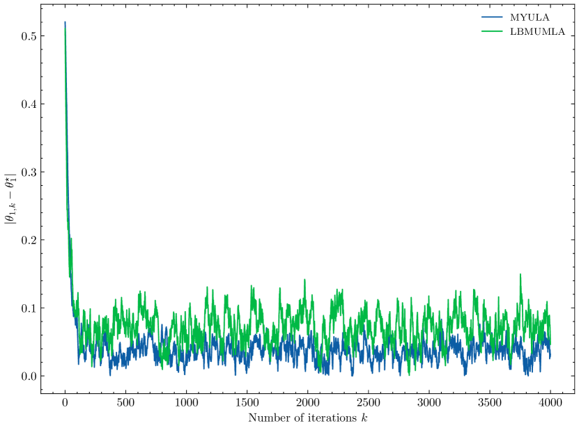
(a) 1^st dimension

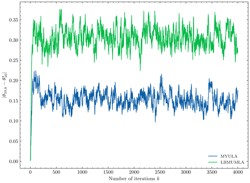
(b) 10^th dimension

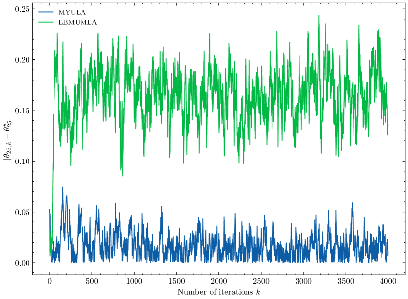
(c) 25^th dimension

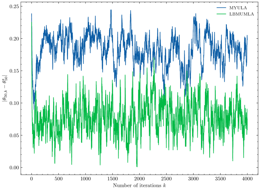
(d) 50^th dimension

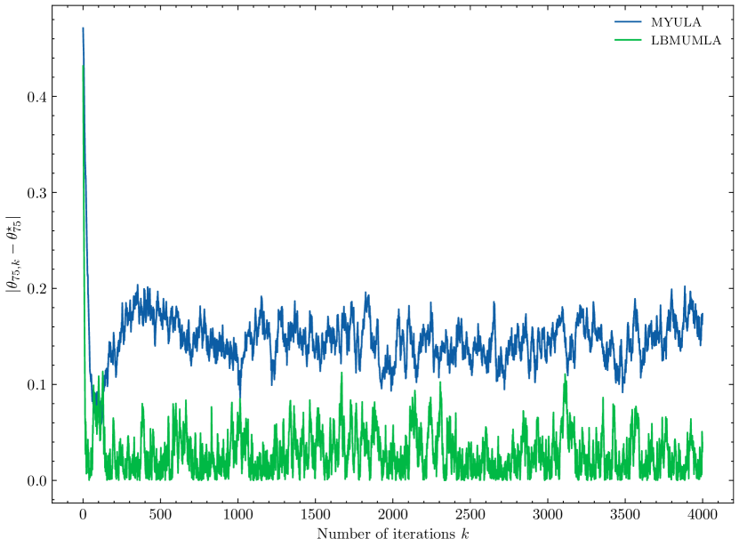
(e) 75^th dimension

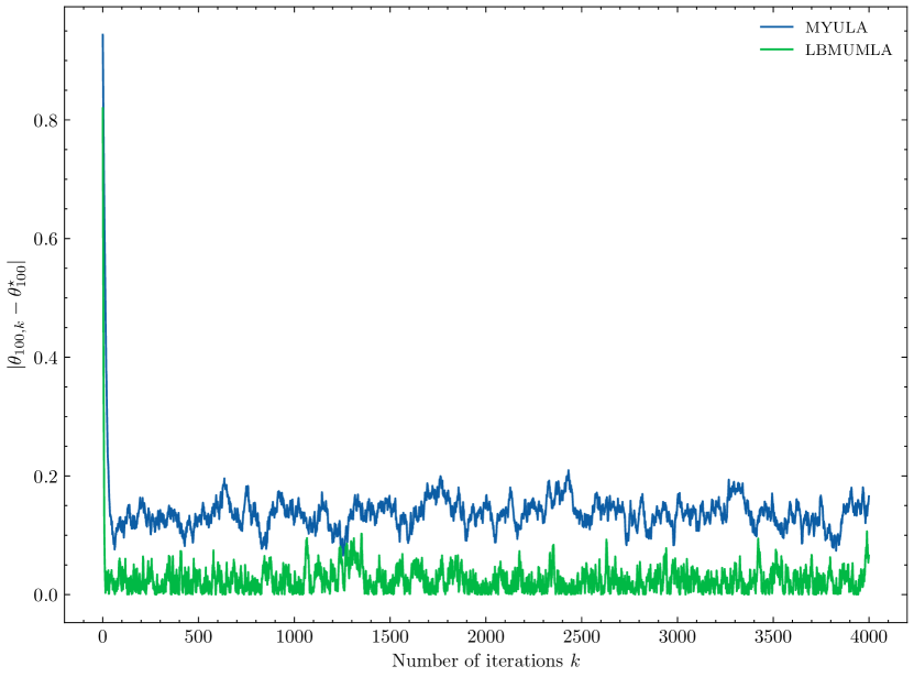
(f) 100^th dimension

Figure D.10: Plots of estimation errors of the posterior means $|\theta_{k,i}-\theta_{i}^{\star}|$ for $i\in\{1,25,50,75,100\}$.

References

- Abdulle et al. (2018) Assyr Abdulle, Ibrahim Almuslimani, and Gilles Vilmart. Optimal explicit stabilized integrator of weak order 1 for stiff and ergodic stochastic differential equations. SIAM/ASA Journal on Uncertainty Quantification, 6(2):937–964, 2018.
- Ahn and Chewi (2021) Kwangjun Ahn and Sinho Chewi. Efficient constrained sampling via the mirror-Langevin algorithm. In Advances in Neural Information Processing Systems (NeurIPS), 2021.
- Ahookhosh et al. (2021) Masoud Ahookhosh, Andreas Themelis, and Panagiotis Patrinos. A Bregman forward-backward linesearch algorithm for nonconvex composite optimization: superlinear convergence to nonisolated local minima. SIAM Journal on Optimization, 31(1):653–685, 2021.
- Bauschke (2003) Heinz H. Bauschke. Duality for Bregman projections onto translated cones and affine subspaces. Journal of Approximation Theory, 121(1):1–12, 2003.
- Bauschke and Borwein (1997) Heinz H. Bauschke and Jonathan M. Borwein. Legendre functions and the method of random Bregman projections. Journal of Convex Analysis, 4(1):27–67, 1997.
- Bauschke and Borwein (2001) Heinz H. Bauschke and Jonathan M. Borwein. Joint and separate convexity of the Bregman distance. In Studies in Computational Mathematics, volume 8, pages 23–36. Elsevier, 2001.
- Bauschke and Combettes (2017) Heinz H. Bauschke and Patrick L. Combettes. Convex Analysis and Monotone Operator Theory in Hilbert Spaces. Springer, 2nd edition, 2017.
- Bauschke and Lewis (2000) Heinz H. Bauschke and Adrian S. Lewis. Dykstras algorithm with Bregman projections: A convergence proof. Optimization, 48(4):409–427, 2000.
- Bauschke et al. (2001) Heinz H. Bauschke, Jonathan M. Borwein, and Patrick L. Combettes. Essential smoothness, essential strict convexity, and Legendre functions in Banach spaces. Communications in Contemporary Mathematics, 3(04):615–647, 2001.
- Bauschke et al. (2003) Heinz H. Bauschke, Jonathan M. Borwein, and Patrick L. Combettes. Bregman monotone optimization algorithms. SIAM Journal on Control and Optimization, 42(2):596–636, 2003.
- Bauschke et al. (2006) Heinz H. Bauschke, Patrick L. Combettes, and Dominikus Noll. Joint minimization with alternating Bregman proximity operators. Pacific Journal of Optimization, 2:401–424, 2006.
- Bauschke et al. (2009) Heinz H. Bauschke, Xianfu Wang, Jane Ye, and Xiaoming Yuan. Bregman distances and Chebyshev sets. Journal of Approximation Theory, 159(1):3–25, 2009.
- Bauschke et al. (2017) Heinz H. Bauschke, Jérôme Bolte, and Marc Teboulle. A descent lemma beyond Lipschitz gradient continuity: first-order methods revisited and applications. Mathematics of Operations Research, 42(2):330–348, 2017.
- Bauschke et al. (2018) Heinz H. Bauschke, Minh N. Dao, and Scott B. Lindstrom. Regularizing with Bregman–Moreau envelopes. SIAM Journal on Optimization, 28(4):3208–3228, 2018.
- Bauschke et al. (2019) Heinz H. Bauschke, Jérôme Bolte, Jiawei Chen, Marc Teboulle, and Xianfu Wang. On linear convergence of non-Euclidean gradient methods without strong convexity and Lipschitz gradient continuity. Journal of Optimization Theory and Applications, 182(3):1068–1087, 2019.
- Bierkens et al. (2019) Joris Bierkens, Paul Fearnhead, and Gareth Roberts. The zig-zag process and super-efficient sampling for Bayesian analysis of big data. The Annals of Statistics, 47(3):1288–1320, 2019.
- Blondel et al. (2020) Mathieu Blondel, André F.T. Martins, and Vlad Niculae. Learning with Fenchel-Young losses. Journal of Machine Learning Research, 21(35):1–69, 2020.
- Bolte et al. (2018) Jérôme Bolte, Shoham Sabach, Marc Teboulle, and Yakov Vaisbourd. First order methods beyond convexity and Lipschitz gradient continuity with applications to quadratic inverse problems. SIAM Journal on Optimization, 28(3):2131–2151, 2018.
- Bouchard-Côté et al. (2018) Alexandre Bouchard-Côté, Sebastian J. Vollmer, and Arnaud Doucet. The bouncy particle sampler: A nonreversible rejection-free Markov chain Monte Carlo method. Journal of the American Statistical Association, 113(522):855–867, 2018.
- Bregman (1967) Lev M. Bregman. The relaxation method of finding the common point of convex sets and its application to the solution of problems in convex programming. USSR Computational Mathematics and Mathematical Physics, 7(3):200–217, 1967.
- Brosse et al. (2017) Nicolas Brosse, Alain Durmus, Éric Moulines, and Marcelo Pereyra. Sampling from a log-concave distribution with compact support with proximal Langevin Monte Carlo. In Proceedings of the Conference on Learning Theory (COLT), 2017.
- Bubeck (2015) Sébastien Bubeck. Convex optimization: Algorithms and complexity. Foundations and Trends® in Machine Learning, 8(3-4):231–357, 2015.
- Bubeck et al. (2018) Sébastien Bubeck, Ronen Eldan, and Joseph Lehec. Sampling from a log-concave distribution with projected Langevin Monte Carlo. Discrete & Computational Geometry, 59(4):757–783, 2018.
- Bùi and Combettes (2021) Minh N. Bùi and Patrick L. Combettes. Bregman forward-backward operator splitting. Set-Valued and Variational Analysis, 29(3):583–603, 2021.
- Chatterji et al. (2020) Niladri Chatterji, Jelena Diakonikolas, Michael I. Jordan, and Peter L. Bartlett. Langevin Monte Carlo without smoothness. In Proceedings of the International Conference on Artificial Intelligence and Statistics (AISTATS), 2020.
- Chen et al. (2012) Ying Ying Chen, Chao Kan, and Wen Song. The Moreau envelope function and proximal mapping with respect to the Bregman distances in Banach spaces. Vietnam Journal of Mathematics, 40(2&3):181–199, 2012.
- Cheng et al. (2018a) Xiang Cheng, Niladri S. Chatterji, Yasin Abbasi-Yadkori, Peter L. Bartlett, and Michael I. Jordan. Sharp convergence rates for Langevin dynamics in the nonconvex setting. arXiv preprint arXiv:1805.01648v4, 2018a.
- Cheng et al. (2018b) Xiang Cheng, Niladri S. Chatterji, Peter L. Bartlett, and Michael I. Jordan. Underdamped Langevin MCMC: A non-asymptotic analysis. In Proceedings of the Conference on Learning Theory (COLT), 2018b.
- Chewi et al. (2020) Sinho Chewi, Thibaut Le Gouic, Chen Lu, Tyler Maunu, Philippe Rigollet, and Austin Stromme. Exponential ergodicity of mirror-Langevin diffusions. In Advances in Neural Information Processing Systems (NeurIPS), 2020.
- Chizat (2021) Lénaïc Chizat. Convergence rates of gradient methods for convex optimization in the space of measures. arXiv preprint arXiv:2105.08368, 2021.
- Cordero-Erausquin (2017) Dario Cordero-Erausquin. Transport inequalities for log-concave measures, quantitative forms, and applications. Canadian Journal of Mathematics, 69(3):481–501, 2017.
- Corless et al. (1996) Robert M. Corless, Gaston H. Gonnet, David E.G. Hare, David J. Jeffrey, and Donald E. Knuth. On the lambert W function. Advances in Computational Mathematics, 5(1):329–359, 1996.
- Dalalyan (2017a) Arnak S. Dalalyan. Further and stronger analogy between sampling and optimization: Langevin Monte Carlo and gradient descent. In Proceedings of the Conference on Learning Theory (COLT), 2017a.
- Dalalyan (2017b) Arnak S. Dalalyan. Theoretical guarantees for approximate sampling from smooth and log-concave densities. Journal of the Royal Statistical Society: Series B (Statistical Methodology), 3(79):651–676, 2017b.
- Dragomir et al. (2021a) Radu-Alexandru Dragomir, Alexandre d’Aspremont, and Jérôme Bolte. Quartic first-order methods for low-rank minimization. Journal of Optimization Theory and Applications, 189(2):341–363, 2021a.
- Dragomir et al. (2021b) Radu-Alexandru Dragomir, Adrien B. Taylor, Alexandre d’Aspremont, and Jérôme Bolte. Optimal complexity and certification of Bregman first-order methods. Mathematical Programming, pages 1–43, 2021b.
- Durmus and Moulines (2017) Alain Durmus and Eric Moulines. Nonasymptotic convergence analysis for the unadjusted Langevin algorithm. The Annals of Applied Probability, 27(3):1551–1587, 2017.
- Durmus and Moulines (2019) Alain Durmus and Eric Moulines. High-dimensional Bayesian inference via the unadjusted Langevin algorithm. Bernoulli, 25(4A):2854–2882, 2019.
- Durmus et al. (2018) Alain Durmus, Eric Moulines, and Marcelo Pereyra. Efficient Bayesian computation by proximal Markov chain Monte Carlo: when Langevin meets Moreau. SIAM Journal on Imaging Sciences, 11(1):473–506, 2018.
- Durmus et al. (2019) Alain Durmus, Szymon Majewski, and Błażej Miasojedow. Analysis of Langevin Monte Carlo via convex optimization. Journal of Machine Learning Research, 20(73):1–46, 2019.
- Eftekhari et al. (2022) Armin Eftekhari, Luis Vargas, and Konstantinos Zygalakis. The forward-backward envelope for sampling with the overdamped Langevin algorithm. arXiv preprint arXiv:2201.09096, 2022.
- Ghai et al. (2020) Udaya Ghai, Elad Hazan, and Yoram Singer. Exponentiated gradient meets gradient descent. In Proceedings of the International Conference on Algorithmic Learning Theory (ALT), 2020.
- Gibbs and Su (2002) Alison L. Gibbs and Francis Edward Su. On choosing and bounding probability metrics. International Statistical Review, 70(3):419–435, 2002.
- Girolami and Calderhead (2011) Mark Girolami and Ben Calderhead. Riemann manifold Langevin and Hamiltonian Monte Carlo methods. Journal of the Royal Statistical Society: Series B (Statistical Methodology), 73(2):123–214, 2011.
- Gunasekar et al. (2021) Suriya Gunasekar, Blake Woodworth, and Nathan Srebro. Mirrorless mirror descent: A more natural discretization of Riemannian gradient flow. In Proceedings of the International Conference on Artificial Intelligence and Statistics (AISTATS), 2021.
- Hanzely et al. (2021) Filip Hanzely, Peter Richtarik, and Lin Xiao. Accelerated Bregman proximal gradient methods for relatively smooth convex optimization. Computational Optimization and Applications, 79(2):405–440, 2021.
- Hsieh et al. (2018) Ya-Ping Hsieh, Ali Kavis, Paul Rolland, and Volkan Cevher. Mirrored Langevin dynamics. In Advances in Neural Information Processing Systems (NeurIPS), 2018.
- Jiang (2021) Qijia Jiang. Mirror Langevin Monte Carlo: the case under isoperimetry. In Advances in Neural Information Processing Systems (NeurIPS), 2021.
- Kan and Song (2012) Chao Kan and Wen Song. The Moreau envelope function and proximal mapping in the sense of the Bregman distance. Nonlinear Analysis: Theory, Methods & Applications, 75(3):1385–1399, 2012.
- Lambert (1758) Johann Heinrich Lambert. Observationes variae in mathesin puram. Acta Helvetica, 3:128–168, 1758.
- Laude et al. (2020) Emanuel Laude, Peter Ochs, and Daniel Cremers. Bregman proximal mappings and Bregman–Moreau envelopes under relative prox-regularity. Journal of Optimization Theory and Applications, 184(3):724–761, 2020.
- Lee et al. (2021) Yin Tat Lee, Ruoqi Shen, and Kevin Tian. Structured logconcave sampling with a restricted Gaussian oracle. In Proceedings of the Conference on Learning Theory (COLT), 2021.
- Lehec (2021) Joseph Lehec. The Langevin Monte Carlo algorithm in the non-smooth log-concave case. arXiv preprint arXiv:2101.10695, 2021.
- Li et al. (2022) Ruilin Li, Molei Tao, Santosh S. Vempala, and Andre Wibisono. The mirror Langevin algorithm converges with vanishing bias. In Proceedings of the International Conference on Algorithmic Learning Theory (ALT), 2022.
- Liang and Chen (2021) Jiaming Liang and Yongxin Chen. A proximal algorithm for sampling from non-smooth potentials. arXiv preprint arXiv:2110.04597, 2021.
- Luu et al. (2021) Tung Duy Luu, Jalal Fadili, and Christophe Chesneau. Sampling from non-smooth distributions through Langevin diffusion. Methodology and Computing in Applied Probability, 23(4):1173–1201, 2021.
- Mangoubi and Vishnoi (2019) Oren Mangoubi and Nisheeth K. Vishnoi. Nonconvex sampling with the Metropolis-adjusted Langevin algorithm. In Proceedings of the Conference on Learning Theory (COLT), 2019.
- Moreau (1962) Jean-Jacques Moreau. Fonctions convexes duales et points proximaux dans un espace hilbertien. Comptes Rendus Hebdomadaires des Séances de l’Académie des Sciences, 255:2897–2899, 1962.
- Moreau (1965) Jean-Jacques Moreau. Proximité et dualité dans un espace hilbertien. Bulletin de la Société Mathématique de France, 93:273–299, 1965.
- Mou et al. (2019) Wenlong Mou, Nicolas Flammarion, Martin J. Wainwright, and Peter L. Bartlett. An efficient sampling algorithm for non-smooth composite potentials. arXiv preprint arXiv:1910.00551, 2019.
- Neal (1993) Radford M. Neal. Bayesian learning via stochastic dynamics. In Advances in Neural Information Processing Systems (NeurIPS), 1993.
- Nemeth and Fearnhead (2021) Christopher Nemeth and Paul Fearnhead. Stochastic gradient Markov chain Monte Carlo. Journal of the American Statistical Association, 116(533):433–450, 2021.
- Nemirovski (1979) Arkadi S. Nemirovski. Efficient methods for large-scale convex optimization problems. Ekonomika i Matematicheskie Metody, 15(1), 1979.
- Nemirovski and Yudin (1983) Arkadi S. Nemirovski and David B. Yudin. Problem Complexity and Method Efficiency in Optimization. John Wiley & Sons, 1983.
- Nesterov (2018) Yurii Nesterov. Lectures on Convex Optimization, volume 137 of Springer Optimization and Its Applications. Springer, 2nd edition, 2018.
- Pereyra (2016) Marcelo Pereyra. Proximal Markov chain Monte Carlo algorithms. Statistics and Computing, 26(4):745–760, 2016.
- Pereyra et al. (2020) Marcelo Pereyra, Luis Vargas Mieles, and Konstantinos C. Zygalakis. Accelerating proximal Markov chain Monte Carlo by using an explicit stabilized method. SIAM Journal on Imaging Sciences, 13(2):905–935, 2020.
- Raginsky et al. (2017) Maxim Raginsky, Alexander Rakhlin, and Matus Telgarsky. Non-convex learning via stochastic gradient Langevin dynamics: a nonasymptotic analysis. In Proceedings of the Conference on Learning Theory (COLT), 2017.
- Roberts and Tweedie (1996) Gareth O. Roberts and Richard L. Tweedie. Exponential convergence of Langevin distributions and their discrete approximations. Bernoulli, 2(4):341–363, 1996.
- Rockafellar (1970) Ralph Tyrell Rockafellar. Convex Analysis. Princeton University Press, Princeton, NJ, 1970.
- Rockafellar and Wets (1998) Ralph Tyrell Rockafellar and Roger J.-B. Wets. Variational Analysis. Springer, 1998.
- Salim and Richtárik (2020) Adil Salim and Peter Richtárik. Primal dual interpretation of the proximal stochastic gradient Langevin algorithm. In Advances in Neural Information Processing Systems (NeurIPS), 2020.
- Salim et al. (2019) Adil Salim, Dmitry Kovalev, and Peter Richtárik. Stochastic proximal Langevin algorithm: Potential splitting and nonasymptotic rates. In Advances in Neural Information Processing Systems (NeurIPS), 2019.
- Soueycatt et al. (2020) Mohamed Soueycatt, Yara Mohammad, and Yamar Hamwi. Regularization in Banach spaces with respect to the Bregman distance. Journal of Optimization Theory and Applications, 185(2):327–342, 2020.
- Takahashi et al. (2021) Shota Takahashi, Mituhiro Fukuda, and Mirai Tanaka. New Bregman proximal type algorithms for solving DC optimization problems. arXiv preprint arXiv:2105.04873, 2021.
- Teboulle (2018) Marc Teboulle. A simplified view of first order methods for optimization. Mathematical Programming, 170(1):67–96, 2018.
- Van Nguyen (2017) Quang Van Nguyen. Forward-backward splitting with Bregman distances. Vietnam Journal of Mathematics, 45(3):519–539, 2017.
- Vempala and Wibisono (2019) Santosh S. Vempala and Andre Wibisono. Rapid convergence of the unadjusted Langevin algorithm: Isoperimetry suffices. In Advances in Neural Information Processing Systems (NeurIPS), 2019.
- Vorstrup Goldman et al. (2021) Jacob Vorstrup Goldman, Torben Sell, and Sumeetpal Sidhu Singh. Gradient-based Markov chain Monte Carlo for Bayesian inference with non-differentiable priors. Journal of the American Statistical Association, pages 1–12, 2021.
- Welling and Teh (2011) Max Welling and Yee Whye Teh. Bayesian learning via stochastic gradient Langevin dynamics. In Proceedings of the International Conference on Machine Learning (ICML), 2011.
- Wibisono (2019) Andre Wibisono. Proximal Langevin algorithm: Rapid convergence under isoperimetry. arXiv preprint arXiv:1911.01469, 2019.
- Zhang et al. (2020) Kelvin Shuangjian Zhang, Gabriel Peyré, Jalal Fadili, and Marcelo Pereyra. Wasserstein control of mirror Langevin Monte Carlo. In Proceedings of the Conference on Learning Theory (COLT), 2020.