Balancing Producer Fairness and Efficiency via Prior-Weighted Rating System Design

Abstract.

Online marketplaces use rating systems to promote the discovery of high-quality products. However, these systems also lead to high variance in producers’ economic outcomes: a new producer who sells high-quality items, may unluckily receive one low rating early on, negatively impacting their future popularity. We investigate the design of rating systems that balance the goals of identifying high-quality products (“efficiency”) and minimizing the variance in economic outcomes of producers of similar quality (individual “producer fairness”).

We show that there is a trade-off between these two goals: rating systems that promote efficiency are necessarily less individually fair to producers. We introduce prior-weighted rating systems as an approach to managing this trade-off. Informally, the system we propose sets a system-wide prior for the quality of an incoming product; subsequently, the system updates that prior to a posterior for each producer’s quality based on user-generated ratings over time. We show theoretically that in markets where products accrue reviews at an equal rate, the strength of the rating system’s prior determines the operating point on the identified trade-off: the stronger the prior, the more the marketplace discounts early ratings data (increasing individual fairness), but the slower the platform is in learning about true item quality (so efficiency suffers). We further analyze this trade-off in a responsive market where customers make decisions based on historical ratings. Through calibrated simulations, we show that the choice of prior strength mediates the same efficiency-consistency trade-off in this setting. Overall, we demonstrate that by tuning the prior as a design choice in a prior-weighted rating system, platforms can be intentional about the balance between efficiency and producer fairness.

1. Introduction

Online marketplaces are mediated by ratings such as star ratings: e.g., . These ratings influence consumer choices, which in turn drive producer economic outcomes. In this paper, we study the impact of rating system design on producers’ welfare. Conditional on item quality, ratings and reviews may be noisy or depend on factors outside the producer’s control (Salganik et al., 2006). This variance in ratings translates into a substantial variance in producer experiences on platforms, especially early on in a producer’s tenure: for example, on eBay, a seller’s first negative rating is associated with a substantial drop in that seller’s growth rate on the platform (Cabral and Hortacsu, 2010). Neglecting this variance in producers’ economic experience can be detrimental to the market: in online labor marketplaces, many highly effective workers are underutilized simply due to a lack of previous experience on the platform (Pallais, 2014). We view this variance in producer outcomes as a form of individual producer unfairness: conditional on true producer quality, outcomes may differ substantially between producers. On the other hand, platforms are also trying to simultaneously learn about and highlight products that are considered to be high quality by consumers, with the goal of matching consumers to as many high-quality products as possible. We refer to this goal of optimizing for consumer experience as efficiency.

Historically, platforms have tried to balance noisy ratings for low-review products and consumer efficiency through the use of Bayesian ratings, which calculates the rating of a product as a weighted average of their review score and an existing fixed value (usually the average rating across all products). Some platforms, like IMDB’s former ratings system (IMDB, 2019), highly weight the fixed value, minimizing the influence noisy ratings have on outcomes for producers of similar true quality, but also making products with a low number of reviews look similar, regardless of their true quality. On the other extreme, some platforms like Uber make the rating for each item the sample mean of their reviews (Uber, 2023), essentially choosing to put zero weight on the fixed value of the Bayesian rating. Under this paradigm, higher-quality products consistently achieve more visibility over time, but the noisy procedure of review generation induces high variance in producer experiences.

The preceding discussion suggests a qualitative trade-off between consumer experience (efficiency) and producer variance (unfairness), as mediated by the choice of rating system: If the fixed value in Bayesian ratings is thought of as a Bayesian prior over item quality, then the choice of prior strength in the rating system has a first-order impact on both the experience of consumers and the variance in producer outcomes. Platforms setting their fixed value under Bayesian ratings have implicitly made a choice about how much they value consumer experience over producer variance. We argue that platforms should be intentional about design choices like these, given the importance of providing high-quality experiences to consumers and of giving fair treatment to producers. We ask: is there a way for the platform to control this efficiency-unfairness trade-off, i.e., to intentionally determine its “operating point” with respect to this trade-off?

We formalize the design of Bayesian ratings by analyzing a family of prior-weighted rating systems, in which the platform’s rating system computationally behaves as a Bayesian updater of the estimated quality of each product on the platform. In this approach, the choice of the prior is a key design variable that mediates the operating point on the efficiency-fairness tradeoff. In more detail, such a system operates as follows. The platform sets a prior distribution for the quality of new products entering the market; any new product is treated by the rating system as if its underlying quality is drawn from this prior. As ratings data is obtained, the prior is updated to a posterior for each product, as formally specified by Bayes’ rule. Because the prior is an input to the operation of this system, the platform can change the system behavior by changing the prior.

We show that the platform can tune the efficiency-fairness trade-off through its choice of this Bayesian prior. For example, a strong prior (i.e., a Bayesian prior that requires several updates before the distribution it parameterizes significantly changes) would require many ratings to overwhelm, leading to a high-fairness but low-efficiency market. As the prior strength is weakened and the platform places more weight on the user-generated ratings it receives, we eventually recover the standard “sample mean” approach used by platforms that maximizes efficiency at the expense of individual producer fairness.

In this paper, we evaluate prior-weighted rating systems and the prior as a design choice, both theoretically and through calibrated simulations using real ratings data. We first analyze a stylized model in which all products accumulate ratings at a uniform rate. We characterize the efficiency-fairness trade-off as being closely related to the bias-variance trade-off on the mean squared error of product quality estimation; we prove that the prior strength determines the operating point on the trade-off curve. We supplement our theoretical analysis with simulations using a real-world recommender systems dataset (Gao et al., 2022).

We then consider a responsive model, where higher-quality products receive more attention over time. In this model, we formalize the efficiency-fairness trade-off using standard consumer and producer welfare metrics: efficiency depends on whether consumers receive high-quality items, and fairness on whether products of the same underlying true quality receive similar attention. Our findings reflect those of the fixed model: the prior strength determines the platform’s operating point on this trade-off curve.

As demonstrated via both models, our paper’s main takeaway is that the prior choice is a neglected but consequential hyperparameter that serves as a key design lever for online marketplaces, with a first-order impact on the outcomes experienced by producers and consumers; in our responsive model, we find that moving from a ”sample mean” rating system that places zero weight on a prior to one that places minimal weight in the prior reduces producer unfairness by 30% while only decreasing match efficiency by 10%. Many platforms today have implicitly made an extreme choice for their prior weight by using the sample mean of ratings. Our paper shows that between the extremes of using the sample mean and ignoring ratings data completely, there lay designs that largely distinguish products by their true quality while still empirically producing consistent (fair) outcomes on the market.

2. Model

We first describe our model and formally define prior-weighted rating systems within our model. We then introduce two model variants: the fixed model assumes that all products accrue ratings at the same rate, and changing the prior does not impact how the collection of user-generated feedback evolves, while the responsive model relaxes this assumption by modeling consumers as noisily seeking the best product on the market. For each model, we define associated metrics for producer fairness and efficiency.

2.1. Model primitives

Here we describe the basic primitives of our modeling framework.

Products. There is a universe of products $V$. Each product $v\in V$ has an unobserved true quality $q_{v}$, where $0\leq q_{v}\leq 1$.

Binary ratings that accumulate over time. Products accumulate ratings over time, as users interact with and rate products. To capture this phenomenon, we assume the market operates over discrete time periods $t$, and products can receive ratings at each time period. We assume these ratings are binary, i.e., 0 or 1 .

Crucially, the true quality of a product should impact the rating received; we suppose that a rating for product $v$ is Bernoulli($q_{v}$), independent of all other randomness in the system. Since ratings accumulate, we use $S(v,T)$ to denote the set of binary ratings that product $v\in V$ has received after $T$ timesteps have elapsed.

Binary ratings, as opposed to arbitrary categorical ratings, are a simplification for ease of exposition and computational investigation; results qualitatively extend to other settings. We note that this choice captures how many platforms elicit ratings (e.g., in any platform that uses a thumbs-up/thumbs-down system); in other platforms with more than two options, ratings often follow a “J-curve” where users mostly only use the extreme options (Hu et al., 2009).

Prior-weighted rating system. In a prior-weighted rating system, the prior distribution is a design choice of the platform. The system operates by estimating a posterior distribution of the estimated true quality for each product, given the prior and the received ratings on that product.

In this paper, we consider rating systems where the prior represents a Beta distribution. Then, in this setting, the platform chooses the prior Beta distribution parameters $(\hat{\alpha},\hat{\beta})$. We will refer to $\hat{\alpha}+\hat{\beta}$ as the prior strength, as it indicates how strongly the prior is concentrated around its mean (and how many ratings will be needed to “overwhelm”) the prior.

After a given product receives a rating, the platform updates its posterior distribution for the item’s true quality. In our Beta-Bernoulli setting, this posterior distribution of estimated quality for product $v$ at timestep $t$ is a Beta distribution with parameters

$$\alpha =\hat{\alpha}+R(v,t),$$

$$\beta =\hat{\beta}+(|S(v,t)|-R(v,t)),$$

where $R(v,t)\sim\textrm{Binomial}(t,q_{v})$ is the number of positive ratings received by the item so far (and so $|S(v,t)|-R(v,t)$ is the number of negative ratings). We can compute the posterior mean estimated quality for product $v$ at timestep $t$ as:

(1) $$\hat{q}_{\hat{\alpha},\hat{\beta}}(v,t) =\frac{\hat{\alpha}+R(v,t)}{\hat{\alpha}+\hat{\beta}+|S(v,t)|}.$$

As noted above, the platform impacts the operation of a prior-weighted rating system only through the choice of the prior, determined in this setting by $\hat{\alpha}$ and $\hat{\beta}$. There are two aspects of this choice: the shape of the prior, and its strength relative to observed ratings in determining the posterior. In our analysis, we fix the prior shape by relying on market-level data, in a manner inspired by empirical Bayesian statistical methods (Robbins, 1964). Our analysis shows that the strength of the prior then mediates the tradeoff between efficiency and producer fairness.

Formally, to reason about a prior’s strength, we fix a prior shape $(\tilde{\alpha},\tilde{\beta})$, then set $(\hat{\alpha},\hat{\beta})=(\eta\tilde{\alpha},\eta\tilde{\beta})$ for some $\eta\geq 0$, providing us with a single-parameter lever to adjust the strength of the prior. We elaborate on how we calibrate the prior shape in Section 3.2. Note in particular that if $\eta=0$, then the platform simply implements sample averaging to compute the estimated quality of an item.

2.2. Fixed and responsive models

How exactly do binary ratings accumulate over time? We study two models, representing different ways in which customers may interact with items items. We begin with a fixed model in which the products receive ratings at the same rate, regardless of their past ratings. We then study a (more realistic) responsive model in which products with higher ratings receive ratings at higher rates do other products with lower ratings.

Fixed model. In the fixed setting, all products stay in the market for the entire time horizon, and each product $v\in V$, at each timestep $t$, accumulates one rating. In this model, the platform eventually accurately learns the quality of each of the products present, but has noisy estimates for each finite time $t$.

Responsive model. The responsive model differs from the fixed model in two ways: (1) items enter and exit the marketplace over time; (2) items are more likely to receive ratings if they have a higher estimated quality in the rating system. These changes in the responsive model capture selection effects (Acemoglu et al., 2022), in which consumers may react to previous ratings, more often choosing to interact with (and thus rate) items with more positive ratings in the past; these effects are not present in the fixed model.

At each timestep $t$, only a subset $M(t)\subseteq V$ of the products is available for purchase. A single consumer chooses a single product $v(t)$ to purchase and provides a rating on that product, and at the end of the timestep, each product $v\in M(t)$ exits the marketplace with some exogenous probability and is replaced. The customer choice will depend on historical ratings for each available item. In our analysis in Section 4, we will instantiate consumers as Thompson samplers.

2.3. Efficiency and producer fairness metrics

We now develop metrics that capture the two qualitative objectives described above: efficiency, and producer fairness. Informally, efficiency is measured by whether or not the rating system is successfully identifying high-quality products. Individual producer fairness is measured by whether products of similar quality are treated similarly.

Metrics in fixed setting. In the fixed model, we focus primarily on an accuracy measure: the mean-squared error (MSE) of the estimated quality in predicting true quality, defined at timestep $t$ as

(2) $$MSE(\hat{q}_{\eta\tilde{\alpha},\eta\tilde{\beta}})=\frac{\sum_{v\in V}(\hat{q}_{\eta\tilde{\alpha},\eta\tilde{\beta}}(v,t)-q_{v})^{2}}{|V|}.$$

Why MSE? Via the bias-variance decomposition, mean-squared error encodes a metric for efficiency and a metric for producer unfairness. For any product $v$ with true quality $q_{v}$, note:

(3) $$\begin{split}\mathbb{E}[(\hat{q}_{\eta\tilde{\alpha},\eta\tilde{\beta}}(v,t)-q_{v})^{2}|q_{v}]&=\left(\mathbb{E}[\hat{q}_{\eta\tilde{\alpha},\eta\tilde{\beta}}(v,t)|q_{v}]-q_{v}\right)^{2}\\ &\hskip 9.95845pt+\textrm{Var}[\hat{q}_{\eta\tilde{\alpha},\eta\tilde{\beta}}(v,t)|q_{v}].\end{split}$$

When conditioned on a product with given true quality $q_{v}$, the variance component of the MSE (second component on the right-hand side) represents an objective for producer fairness, as the estimator should ideally estimate products of similar true quality similarly, even if that estimated quality is biased. The bias component of MSE is correlated with consumer efficiency; in particular, a rating system that consistently underrates high-quality products or overrates low-quality ones will lead to poor consumer experiences.

Metrics in responsive setting. In the responsive setting, because consumers choose (and rate) higher rated items at higher probabilities, we base our metrics directly off of how often products are selected. We define $l_{v}$ to be the lifespan of a product $v$ in the responsive model. The selection rate of a product $v$ as the fraction of times that it was rated (and thus the fraction of times the product was purchased) during its lifespan, $SR(v):=|S(v,t)|/l_{v}$.

Efficiency. Formally, to measure efficiency, we use total expected regret compared to the best item in the marketplace at each time step:

(4) $$\mathbb{E}\left[\sum_{t=1}^{T}\max_{v\in M(t)}\{q_{v}\}-q_{v(t)}\right].$$

Note that low regret corresponds to high selection rates for high quality products, while ensuring sufficient exploration of low quality products. In real markets, this arises naturally from rating products according to the sample mean, meaning lower prior weights should increase efficiency.

Fairness. To capture variance conditional on quality, our chosen fairness metric is the standard deviation in selection rate given true quality. This individual fairness notion is conditional onquality: items of similar quality ought to be picked at similar rates. Let $\hat{\sigma}(U)$ be the sample standard deviation computed on a set of real-valued numbers $U$. For a fixed true quality $q$, the individual (un)fairness metric is the standard deviation in selection rate conditioned on an item being of that true quality:

(5) $$\hat{\sigma}\left(\{SR(v)|q_{v}=q\}\right).$$

To get a marketplace-level metric of overall producer unfairness, we take the expectation of Equation 5 over true qualities $q$.

Note that we do not use a statistical measure as in the fixed setting for two reasons: (1) As discussed above, the responsive model allows for more direct capture of real-world welfare metrics, and (2) as products are sampled adaptively, quality estimation will inherently be negatively biased (Nie et al., 2018), making mean-squared prediction error a poor metric.

3. The Efficiency-Fairness Tradeoff in the Fixed Model

We first analyze the fixed model, in which all products accrue ratings at the same rate over time. This fixed model illustrates our main ideas in a simple setting. We analyze the trade-off in producer fairness and efficiency through the lens of a familiar objective in machine learning: minimizing mean-squared error (MSE) in predicting true product quality. We first show theoretically that an efficiency-fairness trade-off is ensured in this setting as a consequence of the bias-variance decomposition of MSE in Equation 3. We then illustrate our theoretical results through calibrated simulation.

3.1. Theoretical analysis

We present two theorems that characterize the efficiency-fairness trade-off in our fixed model, where efficiency and fairness are defined through the bias-variance decomposition of mean-squared prediction error as given in Equation 3; proofs of both theorems are available in Appendix A. The first theorem is a theoretical guarantee that as the prior strength $\eta$ increases, efficiency increases but fairness decreases:

Theorem 3.1.

Suppose we have a prior-weighted rating system in the fixed setting with prior parameters $(\eta\tilde{\alpha},\eta\tilde{\beta})$. Fix product $v$ with true quality $q_{v}$ and consider quality estimation after $t$ timesteps.

Then, as $\eta\geq$ 0 increases, (1) squared bias $\left(\mathbb{E}[\hat{q}_{\eta\tilde{\alpha},\eta\tilde{\beta}}(v,t)|q_{v}]-q_{v}\right)^{2}$ is nondecreasing; (2) variance $\textrm{Var}[\hat{q}_{\eta\tilde{\alpha},\eta\tilde{\beta}}(v,t)|q_{v}]$ is strictly decreasing in $\eta$.

Theorem 3.1 establishes the trade-off between fairness and efficiency. As the prior strength of a prior-weighted rating system increases, it is less likely for two identical products to be rated differently, which reduces variance, but the increase in prior strength simultaneously increases estimation bias.

The above theorem characterizes error for a given quality level $q_{v}$ as prior strength changes. We are also interested in how the true quality of the product influences the efficiency and fairness metric, i.e., how the platform estimates quality for different true quality levels. An ideal statistical estimator for quality should have low MSE across all quality levels. Our next theorem characterizes how efficiency and unfairness vary with true product quality:

Theorem 3.2.

Suppose we have a prior-weighted rating system in the fixed setting with prior parameters $(\eta\tilde{\alpha},\eta\tilde{\beta})$. Consider quality estimation after $t$ timesteps.

Then, squared bias as a function of true product quality
$\left(\mathbb{E}[\hat{q}_{\eta\tilde{\alpha},\eta\tilde{\beta}}(v,t)|q_{v}]-q_{v}\right)^{2}$ is convex with a global minimum at $\frac{\tilde{\alpha}}{\tilde{\alpha}+\tilde{\beta}}$, while variance as a function of true quality $\textrm{Var}[\hat{q}_{\eta\tilde{\alpha},\eta\tilde{\beta}}(v,t)|q_{v}]$ is concave with a global maximum at 1/2.

Theorem 3.2 illustrates which products would be favored by increasing $\eta$; in the sample mean setting where $\eta=0$ and the unfairness objective is high, producers of middling true quality have the most variance. This is due to Bernoulli distribution variance being highest around $1/2$. As $\eta$ increases, the estimated quality of products not close to $\frac{\tilde{\alpha}}{\tilde{\alpha}+\tilde{\beta}}$ becomes systematically biased, as the prior moves estimated quality of items toward the prior mean. Thus, products above this value systematically are under-estimated, and products below this value are over-estimated, reducing efficiency. Note that if the prior mean $\frac{\tilde{\alpha}}{\tilde{\alpha}+\tilde{\beta}}$ is calibrated (via a method such as empirical Bayes, which we use in our application below), then this value will correspond to the average product quality.

A key takeaway of this theorem is that the efficiency and producer unfairness metrics as a function of product quality have different shapes; as changes in $\eta$ prioritize one metric over the other, different groups of producers will benefit in terms of both efficiency and fairness.

3.2. Empirical setup

We simulate an idealized marketplace using a real-world dataset. We first use simulations to illustrate our fixed model theory. In the next section, we will reuse this framework to simulate the responsive model, evaluating how different prior-weighted rating systems might perform in a setting closer to practice.

Dataset. We ground our model in real-world data by using the KuaiRec dataset, developed by Gao et al. (2022), to calibrate our simulated marketplaces. KuaiRec provides a dense matrix of user-item interactions on a large video-sharing platform where every user has a watchtime percentage for every video, allowing us to base our simulations on data that is free of selection bias. To convert watchtime into a binary rating, we assume a user liked a video if they watched 40% or more of it, then took the mean like ratio of each product $v$ to calculate its true quality $q_{v}$. This thresholding yields a left-tailed true quality distribution with a mean quality of $0.79$, which resembles a typical market with ratings inflation (Garg and Johari, 2021; Horton and Golden, 2015); see Appendix B for a plot of true quality distribution.

Model calibration. To pick a prior shape ($\tilde{\alpha},\tilde{\beta}$), we make use of the empirical Bayes (EB) method (Robbins, 1964), which provides an approach for computing an estimate of prior parameters across a population. We perform a 60-40 train-test split on the products in the KuaiRec dataset. We use all available ratings data for products in the training set to calibrate ($\tilde{\alpha},\tilde{\beta}$) using EB. The remaining 1,331 products (in the test set) are the universe of products $V$ on which the simulation is run. We are interested in investigating how ratings in the marketplace change over time, so our marketplace is simulated over time; we fix a finite time horizon $T$, and at each timestep $t$, either draw one review for all $v\in V$ in the fixed model, or draw one review for the specific $v\in V$ chosen by the consumer at timestep $t$ in the responsive model.

Fixed model parameters. We set a time horizon of $T=50$, and run our simulations for four different values of $\eta\in\{0,1,10,1000\}$. The first two $\eta$ values correspond to prior-weighted rating systems under the sample mean estimator and the baseline empirical Bayes (EB) estimator respectively. $\eta=10$ corresponds to a setting where the prior is difficult to overcome in early timesteps, but eventually is shifted significantly by ratings data. $\eta=1000$ corresponds to a setting where the posterior is essentially equal to the prior throughout the entire simulation, i.e., ratings data is ignored.

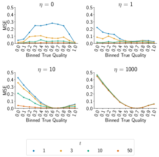
Figure 1. Lineplot representing MSE of different quality estimators in the fixed setting, stratified on true product quality. With few ratings, lower-decile products incur higher MSE with the EB estimator but higher-decile products incur higher error with the sample mean estimator. Note that as $\eta$ increases, the MSE as a function of quality goes from concave, indicating error predominantly comes from variance, to convex, indicating error comes predominantly from bias.

3.3. Empirical results for fixed model

Illustrating the efficiency-fairness trade-off across different values of $\eta$. Overall, our simulations illustrate the theoretical results. Figure 1 plots the estimation MSE as a function of producer true quality, for different levels of $\eta$ and number of timesteps elapsed $t$. Note the shift from concavity to convexity $\eta$ increases – the system shifts from where producer unfairness is the primary contributor to MSE to a system where consumer inefficiency is the main contributor. Figure 2 shows this same phenomenon through plotting estimated versus actual quality; low values of $\eta$ induce high variance in estimation, while high values of $\eta$ induce a systematic bias into the rating system that underestimates high quality products and overestimates low quality ones. Further, by varying prior strength, we can recover both the sample mean estimator where ratings are determined entirely by user reviews, and a ”static” estimator where no amount of data will change a market’s initial assessment of an item. The market designer can thus interpolate between these two extremes by adjusting $\eta$, adjusting the efficiency and producer fairness induced by their rating system. Supplemental visualizations showing how varying $\eta$ impacts aggregate MSE across all products are shown in Appendix B.

No value of $\eta$ is ideal for all products. Our theory and simulations for the fixed model also reveal that there is no estimator in our design space that performs best for all product quality levels in settings with low numbers of reviews; setting low values of $\eta$ ensures that high-quality and low-quality products are accurately identified and treated as such, but induces variance in estimation on products of middling quality. On the other hand, high values of $\eta$ ensure accurate estimation only for products with true qualities close to $\frac{\tilde{\alpha}}{\tilde{\alpha}+\tilde{\beta}}$. This suggests that an “ideal” design that maximizes efficiency and producer fairness cannot be obtained in the fixed model; improving outcomes on one group of products must inherently hurt outcomes on a different group.

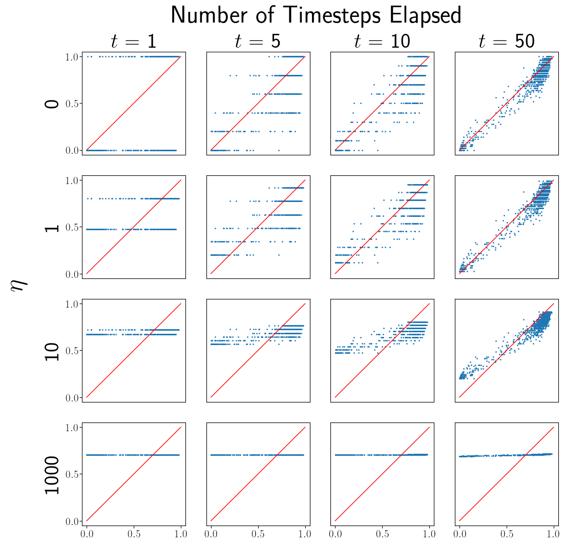
Figure 2. Facet plot showing bias-variance trade-off between quality estimators. The x-axis represents true quality, while the y-axis represents estimated quality. The red line represents a perfectly omniscient estimator. As prior strength $\eta$ increases, the variance of the estimator decreases over all values of $v,t$, but the bias of the estimator increases.

4. Responsive Model

We now analyze the responsive model described in Section 2. This model adds two practical aspects of real-world markets: (1) products stochastically enter and exit, leading to a marketplace where the product offerings change over time and in which the platform is always learning about new products; (2) consumers are more likely to purchase items that have previously received higher ratings. Our responsive model thus resembles a multi-armed bandit with dynamically changing arms and a fixed sampling algorithm, where the market designer influences the information seen by the sampling algorithm. This section is organized as follows. We first outline how we implement simulations for the responsive model, and then investigate how tuning prior strength affects the producer fairness and match quality metrics. We conclude with a discussion of results, and compare our simulation outcomes with those from the fixed model in the previous section.

4.1. Responsive model implementation

Here, we describe our implementation of the responsive model, which we study through calibrated simulation. (Note that, as discussed in Section 2.3, the changes in the responsive setting make quality estimation inherently biased, complicating the theory developed in the fixed setting; Appendix C demonstrates the dependency of bias and variance on the exact dynamics of the sampling algorithm used for consumer choice in this setting.)

An overview of the responsive model’s design and metrics for efficiency and fairness, are provided in Section 2. Our responsive setting simulations use the same KuaiRec dataset and prior shape calibrations from the fixed setting, detailed in Section 3.2. In more detail, our simulation setup is as follows.

Users apply Thompson sampling to products on the market. At each timestep $t$, a subset of the products $M(t)\subseteq V$ is available for purchase. A single user interacts with a single item at each timestep, making their choice as a function of past ratings. In particular, we model this user as a Thompson sampler that utilizes the posterior quality distribution for each item. That is, for each $v\in M(t)$, the consumer draws a sample $x_{v}\sim\textrm{Beta}(\hat{\alpha}+R(v,t),\hat{\beta}+|S(v,t)|-R(v,t))$, and then chooses and rates the product $v(t)$ that maximizes $x_{v}$.

Note that other models of consumer responsive behavior are also appropriate; we make this choice as Thompson sampling is a well-studied algorithm for trading off between exploitation and exploration in multi-armed bandit problems (Russo et al., 2018). Prior work has also argued that it serves as a reasonable approximation of real-world consumer choice; for example, Krafft et al. (2021) demonstrate that when individual human decisions are aggregated together in consumer financial markets, the behavior is remarkably close to that of a distributed Thompson sampling setting.

Rating posterior update. As before, the chosen product $v(t)\in M(t)$ receives binary feedback drawn from a Bernoulli$(q_{v(t)})$ distribution. Using the binary feedback, the Beta distribution associated with it is updated accordingly.

Dynamic product entry and exit. We model products as entering and exiting the marketplace over time, to reflect reality in which real platforms are always in “cold start” with some new products. After an item is chosen and rated at each timestep, each product in the market $v\in M(t)$ independently has some exogenous probability $\rho$ of leaving, and being replaced by a product not in $M(t)$. Let $L(t)$ be the set of products that exit the market at time $t$; a set of products of size $|L(t)|$ is drawn uniformly at random without replacement from $V\setminus M(t)$ to replace the products in $L(t)$. When a product enters the marketplace, it is treated as a new product with zero ratings, even if it had previously been in the market.

Marketplace calibration. We use the same 60-40 product train-test split as in the fixed model simulations, using the training set to calibrate the EB prior as before, and set the market size $|M(t)|$ to be 5 for all timesteps, with a replacement probability of $\rho=0.01$, meaning products will, on average, receive 100 reviews before exiting the market. Because not every product will be in the market at the same time, and only one product is bought at each timestep, we set a time horizon of $T=$ 5,000,000 to make sure enough reviews are generated for each product. For computational efficiency, we further pare down the number of products in the test set: we generate $V$ by resampling 25 products, taking from the test set the $x$th percentile products by quality, where $x\in\{0,4,8,12,16...96\}$.

Prior strength $\eta$. Our focus is investigating how increases in prior strength impact outcomes. We run our simulations with a range of $\eta$ values $\eta\in\{0,1,10,50,100,500,1000\}$. $\eta=0$ and $\eta=1$ correspond to the sample mean and empirical Bayes (EB) estimator respectively, and $\eta=1000$ corresponds to a setting where ratings have little to no impact on estimated quality, with the remaining values allowing us to interpolate between these extremes.

4.2. Results and takeaways

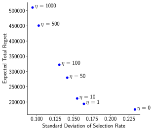
Figure 3. Scatterplot of average standard deviation in selection rate plotted against total expected regret for responsive setting, parameterized by $\eta$. Here, $\eta=0$ represents the sample mean estimator, $\eta=1$ represents the empirical Bayes (EB) estimator. Increasing $\eta$ improves the consistency of producer outcomes, but strictly increases regret.

Prior strength trades off average quality of product sampled with consistency of outcomes for products. As with the fixed model, our results show trade-offs in producer fairness and match quality by varying $\eta$ (Figure 3). With the sample mean estimator, regret (our measure of efficiency) is minimized, but the variance in the percentage of the time a product is purchased while in the market (producer unfairness) is extremely high. Increasing $\eta$ improves the consistency of producer outcomes, but strictly increases regret, with $\eta=1000$ giving maximal aggregate producer fairness while greatly decreasing overall match quality, almost tripling the total regret. We further note that one can substantially reduce producer variance (unfairness) without substantial losses in efficiency, by moving from $\eta=0$ to $\eta=1$ or $\eta=10$. As before, by changing a single parameter in the ratings design, a market designer can interpolate between a market that solely optimizes for consumer efficiency to one that solely optimizes for producer fairness.

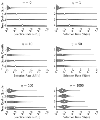
Figure 4. Violin plot of selection rate for products in the responsive setting, faceted by prior strength $\eta$ and stratified on true quality quartile. White dots represent the mean selection rate for each group. At low values of $\eta$, low-quality products consistently get low exposure while high-quality products are popular in expectation, but have high variance in outcome. At high values of $\eta$, all products are consistently purchased at the same rates.

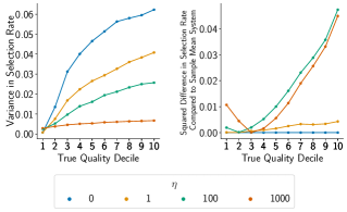
Figure 5. Lineplot of variance in selection rate and squared difference in selection rate from sample mean for the responsive setting, stratified by true quality decile of product. Variance in selection rate is concave and decreases at all levels as $\eta$ increases, while squared difference in selection rate from sample mean is convex and becomes more pronounced as $\eta$ increases.

Improving producer fairness for high-quality products decreases overall match quality. Next, we disaggregate producer fairness across true product quality. Figure 4 demonstrates how the variance in outcomes is distributed across true quality quartiles for different prior strengths. When $\eta$ is 0 or 1 (low prior strength), the mean selection rate for low-quality products is consistently low. On the other hand, high-quality products are on average picked more, but there is substantial variance in the selection rate (high unfairness). As $\eta$ increases, high-quality products are more consistently sampled (lower variance), but so are products of other qualities, and the average selection rate equalizes across all products.

We further investigate the analog to 3.1 and 3.2, how bias and variance vary with the choice of prior. We separate out products by true quality decile, then, within each decile, compute variance in selection rate as our surrogate variance measure. For a measure of bias, for each $\eta$ value and each decile, we take the squared difference of the selection rate in that decile with the selection rate of that decile in the sample mean ($\eta=0$) setting. Figure 5 shows the results of these calculations; we find that our theoretical results conceptually hold in the responsive setting; variance is concave in true quality and decreases as $\eta$ increases, while bias is convex in true quality and increases as $\eta$ increases. These results indicate that as in the fixed setting, low values of $\eta$ cause high producer unfairness for good products, while high values of $\eta$ are inefficient because they overly promote lower-quality products. Across both settings, making sure all products receive similar outcomes as each other comes at a cost of also sustaining low-quality items – as, with a small number of ratings, many low- and high-quality items seem identical to the platform and users.

However, there is a key difference caused by the shift to the responsive model; variance is now highest for high-quality products, especially for small $\eta$. We view this effect as a result of “rich-get-richer” effects in systems where users make decisions based on prior ratings – we explore this phenomenon next.

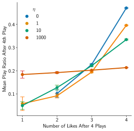
Figure 6. Lineplot showing expected selection rate for products in the highest true quality quartile in remaining lifespan after 4 buys, conditioned on how many of the first 4 buys were likes, plotted for several values of prior strength $\eta$. At low values of $\eta$, products that received more likes early have a much higher mean selection rate than products that received more dislikes early; at high values of $\eta$, this difference vanishes.

Increasing prior strength mitigates rich-get-richer effects. Finally, the results illustrate that higher prior weights can mediate popularity bias. We measured products in the top quartile of true quality within $V$ that stayed in the market long enough to be purchased 4 or more times. We display the mean selection rate of these products conditional on the value of $\eta$ and their number of likes in the first 4 purchases. For low values of $\eta$, early performance has significant consequences on future popularity, with the mean selection rate for the 4-likes group being more than six times that of the 1-like group when $\eta=1$. As $\eta$ increases, the number of likes achieved early on has fewer consequences for future exposure, due to the prior; the mean selection rate for all groups is roughly 0.19 when $\eta=1000$. Our results are illustrated in Figure 6.

This demonstrates a phenomenon of most real-world marketplaces, not captured by the fixed model: when ratings have a large impact on estimated quality, early popularity for a product snowballs demand for that product, even if other products that did not get popular early are of higher quality. Increasing the prior strength helps mitigate snowball effects, as stronger priors require more evidence from early reviews that a product is truly high-quality. Mitigating the effect induces its own trade-off: Figure 4 shows that for high $\eta$ values, lucky breaks in popularity for products happen less, but it also takes more evidence for the system to identify a truly low-quality product as such, replacing the loss in producer fairness from rich-get-richer effects with a loss in match quality.

5. Discussion

5.1. Main contributions

Consistency in outcomes for producers as a key metric of producer fairness in online marketplaces. In each of our fixed and responsive models, we put forward definitions of consumer efficiency and producer fairness that can be applied to online marketplaces where ratings are accrued over time. Our definitions of producer fairness are built around a notion of individual fairness; differing individuals may be treated differently, but similar individuals ought to be treated similarly. We juxtapose our definition of producer fairness with notions of market efficiency for consumers. We frame producer fairness as an objective in its own regard to be designed for, rather than as an impediment to market efficiency.

Prior-weighted rating systems to engineer the trade-off in efficiency and producer fairness. Our primary contribution is the design and analysis of a specific class of prior-weighted rating systems that allows market designers to trade off across variance in producer outcomes and average match quality. The class is parameterized via the choice of prior, which is then updated with data via Bayesian updating. We find that by fixing the shape of the prior and varying the strength, the prior-weighted rating system can achieve a wide range of outcomes, including recovering the commonly used sample mean estimator. Increasing prior strength results in a trade-off between efficiency and producer fairness, where consistency in outcome for high-quality products necessarily requires those high-quality products to have less average exposure.

We prove structural properties of such systems, including how prior strength affects bias and variance of the MSE of quality estimation, and how these systems differentially affect items of different true quality levels. We illustrate these trade-offs with calibrated experiments using a real-world recommender system dataset.

5.2. Future directions

Strategic considerations. We have not considered strategic behavior of market participants in the presence of a prior-weighted rating system, on either the user or producer side.

On the user side, users may choose not to leave ratings (Tadelis, 2016) or leave fake ratings to boost specific producers (Hu et al., 2012; Golrezaei et al., 2021). There may further be limits to how much the platform can vary the prior, as users are likely to respond strategically by ignoring ratings information if they are obviously uninformative. In particular, users who behave according to rational expectations theory may attempt to “correct” quality estimates and impose their own priors, as opposed to using the platform-provided estimates to make choices. More generally, we do not explicitly consider user interface considerations for how such systems can be presented to users.

On the producer side, the producer choice to enter or exit the marketplace is strategic and may depend on the system design (Vellodi, 2018). There may further be considerations in what products to produce, as a function of economic rewards the platform provides (Jagadeesan et al., 2022).

We broadly believe modeling these strategic considerations is an important direction of future research. We expect that even in the presence of these strategic considerations, the same tradeoff between efficiency and producer fairness is likely to be salient for system design; said differently, while we expect strategic considerations to impact the choice of prior-weighted system, we expect that its role in mediating the efficiency-fairness tradeoff is robust.

Real-world considerations. As noted in our model development, we have simplified and abstracted away from many of the complex dynamics of real marketplaces. First, we consider binary ratings in this paper, whereas in real-world systems ratings may have multiple levels (e.g., five stars) across several categories (e.g., shipping speed, seller communication, etc.). Constructing prior-weighted rating systems for these platforms would require higher-dimensional priors (e.g., Dirichlet) and extensions of the procedures described here. Nevertheless, we expect the same qualitative impact of prior strength to apply. Second, we have not considered heterogeneity in producers across the marketplace; in practice, a prior would likely need to account for producer covariates that describe distinguishing features, like product category. Finally, while we have compared against sample mean rating systems, some platforms in practice will use more complex machine-learning models to determine the displayed ratings. We anticipate a generalization of our theoretical work to still apply to machine learning-powered rating systems: broadly speaking, every rating system has a ”dynamic” component that updates a product’s rating based on the reviews it accrues over time, and a ”static” component that evaluates the product even when it has no reviews, which is analogous to the role of prior strength in a prior-weighted rating system. As such, comparing such “black box” rating systems with the more transparent prior-weighted rating system design proposed here remains an interesting direction for future work.

6. Related Work

6.1. Variance in producer outcomes

Substantial work has shown that online marketplaces driven by user feedback increase the volatility of outcomes for producers. Salganik et al. (2006) demonstrate, in an artificial music recommendation marketplace, that letting users see feedback about how often other users downloaded songs greatly increased the unpredictability of how often songs were downloaded. On eBay, Cabral and Hortacsu (2010) demonstrate that the very first negative review received by a product substantially decreases a seller’s growth rate by 13%, and increases the likelihood they receive even more negative reviews in the future. One reason for such variance is ratings inflation (Filippas et al., 2018; Horton and Golden, 2015; Zervas et al., 2021; Hu et al., 2009), where, in practice, ratings are observed to be extremely high on average; such inflation magnifies the importance of any single negative rating.

The recommender systems literature considers variance in producer outcomes through the lens of popularity bias, where popular items are recommended frequently but niche items that are potentially of high value to customers are rarely recommended (Abdollahpouri, 2019; Elahi et al., 2021). Vellodi (2018) creates a model marketplace where ratings drive exposure for firms who face entry and exit decisions. Variance in the treatment of firms has a detrimental effect on overall market efficiency due to barriers in entry; firms that are truly high-quality may be priced out of the market by a lack of reviews, while lower-quality firms that did get noticed stay in the market. Chen et al. (2022) frame popularity bias in the terms of fair assortment planning in assortment optimization. Interventions to mitigate popularity bias take the form of different recommendation algorithms that leverage techniques such as reweighting (Abdollahpouri et al., 2019) or causal methods (Wei et al., 2021). Metrics for success in mitigating popularity bias are usually based on how often the recommender suggests products in the ”long tail” of exposure while still achieving high recommendation accuracy.

A commonality in these works is that unpredictability in producer variance is undesirable – it leads to high-quality products being frequently underexposed, or lower-quality products remaining on the platform. We consider rating system design to reduce this variance, which we view through the lens of individual fairness.

6.2. Other interventions in rating systems

Other works have developed solutions to tackle uninformative ratings and producer unfairness. Garg and Johari (2019, 2021) consider changing the user interface to deflate the distribution of ratings. Other proposed solutions include aligning rater incentives (Gaikwad et al., 2016; Cabral and Li, 2015; Fradkin and Holtz, 2022). These solutions concern the process by which ratings are provided by customers after a purchase, which we assume is fixed.

Other works, like ours, seek to modify how the platform learns from ratings and, in turn, what it shows users. Acemoglu et al. (2022) consider learning in the presence of selection effects of who leaves ratings, informing the design choice of rating systems that either show the full history of ratings to customers or just their summary statistics. Perhaps the work closest to ours is that of Vellodi (2018), who considers “upper censorship” of ratings that are shown to customers, to mitigate barriers to entry caused by long-lived producers with many ratings. In contrast, we seek to balance producer fairness and consumer efficiency caused by ratings variance, and provide a class of system designs for this trade-off.

6.3. Fairness and incentivizing exploration in multi-armed bandits

We conceptually view rating system design (in particular, how the platform learns quality estimates from ratings data) as one trading off “fairness” (reducing individual producer variance) and efficiency (helping customers find higher-quality items). This view connects our work to the idea of exploration vs exploitation in multi-armed bandits; in particular, we cast consumers as playing the role of regret-minimizing agents who are given a set of products to choose from, based on information provided by the recommendation system. Producer fairness then relates to ideas in fairness in bandits; Joseph et al. (2016) formulate the notion that lower-quality arms should not be favored over higher-quality ones, and Liu et al. (2017); Wang et al. (2021) that consistency-optimizing definitions where similar individuals should be rewarded similarly. Interventions in these settings involve creating novel sampling algorithms; in contrast, our model holds fixed consumer behavior and focuses on modifications to the underlying rating system.

A particular subfield of interest within the multi-armed bandits literature is the literature on incentivizing exploration (Slivkins, 2021), where a principal communicates messages to agents who choose their own actions from among the arms presented to them based on that information. Objectives in this paradigm include maximizing reward despite overly myopic agents by encouraging those agents to explore more (Frazier et al., 2014; Immorlica et al., 2018), or ensuring that all options in the space are explored at least once (Sellke and Slivkins, 2021; Simchowitz and Slivkins, 2021). Our work views increasing exploration not as an instrumental goal to increase the platform’s information about product quality, or greater match quality, but as a pathway to increasing producer fairness. In this way, our paper presents insights about market design that complement objectives in the incentivizing exploration literature.

7. Conclusion

While rating aggregation is often viewed as a fairly unremarkable aspect of marketplace design, it is extremely consequential for the producer experience. A single early bad rating can make it impossible for a product to ever recover, while early successes can fuel a rise. In this paper, we propose that marketplaces ought to engineer these rating systems purposefully, in particular, to control the tradeoff between these fairness considerations and the consumer experience. We demonstrate through a prior-weighted rating system that the choice of prior can strike a balance between these competing goals.

Appendix A Proof of fixed model theorems

See 3.1

Proof.

In the fixed setting with binary ratings, for a product with true quality $q_{v}$, $|S(v,t)|=t$ and $R(v,t)\sim\textrm{Binomial}(t,q_{v})$. We can break down squared bias as follows:

(6) $$(\mathbb{E}[\hat{q}_{\eta\tilde{\alpha},\eta\tilde{\beta}}(v,t)|q_{v}]-q_{v})^{2} =\left(\mathbb{E}\left[\frac{\eta\tilde{\alpha}+R(v,t)}{\eta\tilde{\alpha}+\eta\tilde{\beta}+t}\Biggr{|}q_{v}\right]-q_{v}\right)^{2}$$

(7) $$=\left(\frac{\eta\tilde{\alpha}-\eta\tilde{\alpha}q_{v}-\eta\tilde{\beta}q_{v}}{\eta\tilde{\alpha}+\eta\tilde{\beta}+t}\right)^{2}.$$

Variance can also be broken down accordingly:

(8) $$\textrm{Var}[\hat{q}_{\eta\tilde{\alpha},\eta\tilde{\beta}}(v,t)|q_{v}] =\mathbb{E}\left[\left(\hat{q}_{\eta\tilde{\alpha},\eta\tilde{\beta}}(v,t)-\mathbb{E}[\hat{q}_{\eta\tilde{\alpha},\eta\tilde{\beta}}(v,t)]\right)^{2}\Biggr{|}q_{v}\right]$$

(9) $$=\frac{\mathbb{E}[(R(v,t)-\mathbb{E}[R(v,t)])^{2}|q_{v}]}{(\eta\tilde{\alpha}+\eta\tilde{\beta}+t)^{2}}$$

(10) $$=\frac{\textrm{Var}[R(v,t)|q_{v}]}{(\eta\tilde{\alpha}+\eta\tilde{\beta}+t)^{2}}$$

(11) $$=\frac{tq_{v}(1-q_{v})}{(\eta\tilde{\alpha}+\eta\tilde{\beta}+t)^{2}}.$$

The expected MSE can be written as follows:

$$\textrm{MSE}=\left(\frac{\eta\tilde{\alpha}-\eta\tilde{\alpha}q_{v}-\eta\tilde{\beta}q_{v}}{\eta\tilde{\alpha}+\eta\tilde{\beta}+t}\right)^{2}+\frac{tq_{v}(1-q_{v})}{(\eta\tilde{\alpha}+\eta\tilde{\beta}+t)^{2}}.$$

We now differentiate the bias term with respect to $\eta$:

(12) $$\frac{\partial}{\partial\eta}\left(\frac{\eta\tilde{\alpha}-\eta\tilde{\alpha}q_{v}-\eta\tilde{\beta}q_{v}}{\eta\tilde{\alpha}+\eta\tilde{\beta}+t}\right)^{2} \propto\frac{\partial}{\partial\eta}\frac{\eta^{2}}{(\eta(\tilde{\alpha}+\tilde{\beta})+t)^{2}}$$

(13) $$=\frac{2\eta t^{2}}{(\eta(\tilde{\alpha}+\tilde{\beta})+t)^{4}}.$$

This value is clearly positive for all $\eta>0$ and 0 at $\eta=0$, indicating the value of the bias term does indeed strictly increase when $\eta$ increases, while being nondecreasing at $\eta=0$.

Similarly, we differentiate the variance term with respect to $\eta$:

(14) $$\frac{\partial}{\partial\eta}\frac{tq_{v}(1-q_{v})}{(\eta\tilde{\alpha}+\eta\tilde{\beta}+t)^{2}} \propto\frac{\partial}{\partial\eta}\frac{1}{(\eta\tilde{\alpha}+\eta\tilde{\beta}+t)^{2}}$$

(15) $$=\frac{-2(\tilde{\alpha}+\tilde{\beta})}{(\eta\tilde{\alpha}+\eta\tilde{\beta}+t)^{3}}.$$

This demonstrates that variance is always strictly decreasing for $\eta\geq 0.$

∎

See 3.2

Proof.

Using the expression of variance derived in Equation 11, it is evident that the error from variance takes on a concave shape with a global maximum at 1/2 when interpreted as a function of $q_{v}$. To conclude the proof it suffices to show that the bias term derived in Equation 7 is convex and has global minimum $\frac{\tilde{\alpha}}{\tilde{\alpha}+\tilde{\beta}}$ when interpreted as a function of $q_{v}$. We begin again by differentiating:

(16) $$\frac{\partial}{\partial q_{v}}(\mathbb{E}[\hat{q}_{\eta\tilde{\alpha},\eta\tilde{\beta}}(v,t)|q_{v}]-q_{v})^{2} =\frac{\partial}{\partial q_{v}}\left(\frac{\eta\tilde{\alpha}+tq_{v}}{\eta\tilde{\alpha}+\eta\tilde{\beta}+t}-q_{v}\right)^{2}$$

(17) $$\propto-2\left(\frac{\eta\tilde{\alpha}-\eta\tilde{\alpha}q_{v}-\eta\tilde{\beta}q_{v}}{\eta\tilde{\alpha}+\eta\tilde{\beta}+t}\right).$$

This final term is negative when $q_{v}<\frac{\tilde{\alpha}}{\tilde{\alpha}+\tilde{\beta}}$, positive when $q_{v}>\frac{\tilde{\alpha}}{\tilde{\alpha}+\tilde{\beta}}$, and zero at equality, implying a local minimum at $\frac{\tilde{\alpha}}{\tilde{\alpha}+\tilde{\beta}}$.

To prove convexity, note that

(18) $$\frac{\partial^{2}}{\partial q_{v}^{2}}(\mathbb{E}[\hat{q}_{\eta\tilde{\alpha},\eta\tilde{\beta}}(v,t)|q_{v}]-q_{v})^{2} \propto 2\left(\frac{\eta\tilde{\alpha}+\eta\tilde{\beta}}{\eta\tilde{\alpha}+\eta\tilde{\beta}+t}\right)\geq 0,$$

indicating the function is convex. ∎

Appendix B Supplemental Visualizations

This appendix contains supplemental graphs from our calibrated simulations.

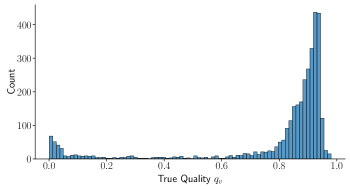
Figure 7. Histogram of true quality distribution of products in the KuaiRec dataset. Note the long left tail and high concentration of products with a quality of 0.7-0.9.

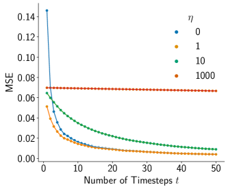
Figure 8. Lineplot of mean-squared error different quality estimators in fixed setting over time. $\eta=0$ represents the sample mean estimator, $\eta=1$ represents the empirical Bayes (EB) estimator. The sample mean estimator ($\eta=0$) has high MSE for low time-steps, due to variance in ratings. On the other extreme, for extremely high prior strength $\eta=1000$, the platform never learns from ratings data. This presents evidence that proper calibration of prior strength can help solve the cold start problem in the context of accurate quality estimates for products.

Appendix C Discussion of bias-variance decomposition in responsive model

This appendix discusses a decomposition of the bias-variance decomposition in Equation 7 as applied to the responsive setting. While mean-squared prediction error may no longer serve as an ideal metric for consumer and producer welfare in this setting, we demonstrate that markets that care about MSE for its own sake can still reason about prediction error for a prior-weighted rating system so long as they can make statements about the changes in how products are sampled based on changes in $q_{v}$ and $\eta$.

Let the number of reviews for product $v$ with fixed true quality $q_{v}$, prior parameters $\tilde{\alpha},\tilde{\beta}$ and system-level prior strength $\eta$, calculated at timestep $t$, be $N_{\tilde{\alpha},\tilde{\beta}}(q_{v},\eta,t)$. We focus on the number of reviews for a product at a fixed time $t$ with fixed prior parameters $\tilde{\alpha},\tilde{\beta}$, and so we simplify by omitting these variables in this notation, letting $N(q_{v},\eta)$ denote the number of reviews. Now, at this time $t$, a prior-weighted rating system’s estimated quality for $v$ is given by $\hat{q}_{\eta\tilde{\alpha},\eta\tilde{\beta}}(v,N(q_{v},\eta))$, and the MSE is given by $\mathbb{E}[(\hat{q}_{\eta\tilde{\alpha},\eta\tilde{\beta}}(v,N(q_{v},\eta))-q_{v})^{2}|q_{v}]$. We can break down bias and variance of mean-squared prediction error through the usage of the tower law of probability:

(19) $$\mathbb{E}[(\hat{q}_{\eta\tilde{\alpha},\eta\tilde{\beta}}(v,N(q_{v},\eta))-q_{v})^{2}|q_{v}]\\ =\mathbb{E}\left[\mathbb{E}[(\hat{q}_{\eta\tilde{\alpha},\eta\tilde{\beta}}(v,N(q_{v},\eta))-q_{v})^{2}]\big{|}N(q_{v},\eta),q_{v}\right]$$

When the number of reviews at a given point in time is fixed, we can treat the estimated quality identically to how it is calculated in the fixed setting. This gives us the following bias-variance breakdown:

(20) $$\mathbb{E}[(\hat{q}_{\eta\tilde{\alpha},\eta\tilde{\beta}}(v,N(q_{v},\eta))-q_{v})^{2}|q_{v}]\\ =\mathbb{E}\left[\left(\frac{\eta\tilde{\alpha}-\eta\tilde{\alpha}q_{v}-\eta\tilde{\beta}q_{v}}{\eta\tilde{\alpha}+\eta\tilde{\beta}+N(q_{v},\eta)}\right)^{2}\Biggr{|}q_{v}\right]+\mathbb{E}\left[\frac{N(q_{v},\eta)q_{v}(1-q_{v})}{(\eta\tilde{\alpha}+\eta\tilde{\beta}+N(q_{v},\eta))^{2}}\Biggr{|}q_{v}\right]$$

From here, one may proceed with the proofs of the theorems in Section 3 so long as they can make statements about the bias and variance terms in the above expression. In the responsive model in this paper, $N(q_{v},\eta)$ is a noisy random variable that is a function of the play distribution in a multi-armed bandit; however, for other responsive marketplaces with simpler number-of-reviews functions, we can characterize how accurate prior-weighted rating systems are through analysis of this equation.

References

- (1)
- Abdollahpouri (2019) Himan Abdollahpouri. 2019. Popularity bias in ranking and recommendation. In Proceedings of the 2019 AAAI/ACM Conference on AI, Ethics, and Society. 529–530.
- Abdollahpouri et al. (2019) Himan Abdollahpouri, Robin Burke, and Bamshad Mobasher. 2019. Managing popularity bias in recommender systems with personalized re-ranking. In The thirty-second international flairs conference.
- Acemoglu et al. (2022) Daron Acemoglu, Ali Makhdoumi, Azarakhsh Malekian, and Asuman Ozdaglar. 2022. Learning from reviews: The selection effect and the speed of learning. Econometrica 90, 6 (2022), 2857–2899.
- Cabral and Hortacsu (2010) Luis Cabral and Ali Hortacsu. 2010. The dynamics of seller reputation: Evidence from eBay. The Journal of Industrial Economics 58, 1 (2010), 54–78.
- Cabral and Li (2015) Luis Cabral and Lingfang Li. 2015. A dollar for your thoughts: Feedback-conditional rebates on eBay. Management Science 61, 9 (2015), 2052–2063.
- Chen et al. (2022) Qinyi Chen, Negin Golrezaei, Fransisca Susan, and Edy Baskoro. 2022. Fair assortment planning. arXiv preprint arXiv:2208.07341 (2022).
- Elahi et al. (2021) Mehdi Elahi, Danial Khosh Kholgh, Mohammad Sina Kiarostami, Sorush Saghari, Shiva Parsa Rad, and Marko Tkalčič. 2021. Investigating the impact of recommender systems on user-based and item-based popularity bias. Information Processing & Management 58, 5 (2021), 102655.
- Filippas et al. (2018) Apostolos Filippas, John Joseph Horton, and Joseph Golden. 2018. Reputation inflation. In Proceedings of the 2018 ACM Conference on Economics and Computation. 483–484.
- Fradkin and Holtz (2022) Andrey Fradkin and David Holtz. 2022. Do incentives to review help the market? Evidence from a field experiment on Airbnb. American Economic Review: Insights (2022).
- Frazier et al. (2014) Peter Frazier, David Kempe, Jon Kleinberg, and Robert Kleinberg. 2014. Incentivizing exploration. In Proceedings of the fifteenth ACM conference on Economics and computation. 5–22.
- Gaikwad et al. (2016) Snehalkumar (Neil) S Gaikwad, Durim Morina, Adam Ginzberg, Catherine Mullings, Shirish Goyal, Dilrukshi Gamage, Christopher Diemert, Mathias Burton, Sharon Zhou, Mark Whiting, et al. 2016. Boomerang: Rebounding the consequences of reputation feedback on crowdsourcing platforms. In Proceedings of the 29th Annual Symposium on User Interface Software and Technology. 625–637.
- Gao et al. (2022) Chongming Gao, Shijun Li, Wenqiang Lei, Jiawei Chen, Biao Li, Peng Jiang, Xiangnan He, Jiaxin Mao, and Tat-Seng Chua. 2022. KuaiRec: A Fully-observed Dataset and Insights for Evaluating Recommender Systems. In Proceedings of the 31st ACM International Conference on Information and Knowledge Management (Atlanta, GA, USA) (CIKM ’22). 11 pages. https://doi.org/10.1145/3511808.3557220
- Garg and Johari (2019) Nikhil Garg and Ramesh Johari. 2019. Designing optimal binary rating systems. In The 22nd International Conference on Artificial Intelligence and Statistics. PMLR, 1930–1939.
- Garg and Johari (2021) Nikhil Garg and Ramesh Johari. 2021. Designing informative rating systems: Evidence from an online labor market. Manufacturing & Service Operations Management 23, 3 (2021), 589–605.
- Golrezaei et al. (2021) Negin Golrezaei, Vahideh Manshadi, Jon Schneider, and Shreyas Sekar. 2021. Learning product rankings robust to fake users. In Proceedings of the 22nd ACM Conference on Economics and Computation. 560–561.
- Horton and Golden (2015) J Horton and J Golden. 2015. Reputation inflation in an online marketplace. New York I 1 (2015).
- Hu et al. (2012) Nan Hu, Indranil Bose, Noi Sian Koh, and Ling Liu. 2012. Manipulation of online reviews: An analysis of ratings, readability, and sentiments. Decision support systems 52, 3 (2012), 674–684.
- Hu et al. (2009) Nan Hu, Jie Zhang, and Paul A Pavlou. 2009. Overcoming the J-shaped distribution of product reviews. Commun. ACM 52, 10 (2009), 144–147.
- IMDB (2019) IMDB. 2019. IMDB Help Center. https://web.archive.org/web/20191106153526/https://help.imdb.com/article/imdb/track-movies-tv/ratings-faq/G67Y87TFYYP6TWAV#
- Immorlica et al. (2018) Nicole Immorlica, Jieming Mao, Aleksandrs Slivkins, and Zhiwei Steven Wu. 2018. Incentivizing exploration with selective data disclosure. arXiv preprint arXiv:1811.06026 (2018).
- Jagadeesan et al. (2022) Meena Jagadeesan, Nikhil Garg, and Jacob Steinhardt. 2022. Supply-side equilibria in recommender systems. arXiv preprint arXiv:2206.13489 (2022).
- Joseph et al. (2016) Matthew Joseph, Michael Kearns, Jamie H Morgenstern, and Aaron Roth. 2016. Fairness in learning: Classic and contextual bandits. Advances in neural information processing systems 29 (2016).
- Krafft et al. (2021) Peter M Krafft, Erez Shmueli, Thomas L Griffiths, Joshua B Tenenbaum, et al. 2021. Bayesian collective learning emerges from heuristic social learning. Cognition 212 (2021), 104469.
- Liu et al. (2017) Yang Liu, Goran Radanovic, Christos Dimitrakakis, Debmalya Mandal, and David C Parkes. 2017. Calibrated fairness in bandits. arXiv preprint arXiv:1707.01875 (2017).
- Nie et al. (2018) Xinkun Nie, Xiaoying Tian, Jonathan Taylor, and James Zou. 2018. Why adaptively collected data have negative bias and how to correct for it. In International Conference on Artificial Intelligence and Statistics. PMLR, 1261–1269.
- Pallais (2014) Amanda Pallais. 2014. Inefficient hiring in entry-level labor markets. American Economic Review 104, 11 (2014), 3565–99.
- Robbins (1964) Herbert Robbins. 1964. The empirical Bayes approach to statistical decision problems. The Annals of Mathematical Statistics 35, 1 (1964), 1–20.
- Russo et al. (2018) Daniel J Russo, Benjamin Van Roy, Abbas Kazerouni, Ian Osband, Zheng Wen, et al. 2018. A tutorial on thompson sampling. Foundations and Trends® in Machine Learning 11, 1 (2018), 1–96.
- Salganik et al. (2006) Matthew J Salganik, Peter Sheridan Dodds, and Duncan J Watts. 2006. Experimental study of inequality and unpredictability in an artificial cultural market. science 311, 5762 (2006), 854–856.
- Sellke and Slivkins (2021) Mark Sellke and Aleksandrs Slivkins. 2021. The price of incentivizing exploration: A characterization via thompson sampling and sample complexity. In Proceedings of the 22nd ACM Conference on Economics and Computation. 795–796.
- Simchowitz and Slivkins (2021) Max Simchowitz and Aleksandrs Slivkins. 2021. Exploration and incentives in reinforcement learning. arXiv preprint arXiv:2103.00360 (2021).
- Slivkins (2021) Aleksandrs Slivkins. 2021. Exploration and persuasion.
- Tadelis (2016) Steven Tadelis. 2016. Reputation and feedback systems in online platform markets. Annual Review of Economics 8 (2016), 321–340.
- Uber (2023) Uber. 2023. How Star Ratings Work. https://www.uber.com/ca/en/drive/basics/how-ratings-work/
- Vellodi (2018) Nikhil Vellodi. 2018. Ratings design and barriers to entry. Available at SSRN 3267061 (2018).
- Wang et al. (2021) Lequn Wang, Yiwei Bai, Wen Sun, and Thorsten Joachims. 2021. Fairness of exposure in stochastic bandits. In International Conference on Machine Learning. PMLR, 10686–10696.
- Wei et al. (2021) Tianxin Wei, Fuli Feng, Jiawei Chen, Ziwei Wu, Jinfeng Yi, and Xiangnan He. 2021. Model-agnostic counterfactual reasoning for eliminating popularity bias in recommender system. In Proceedings of the 27th ACM SIGKDD Conference on Knowledge Discovery & Data Mining. 1791–1800.
- Zervas et al. (2021) Georgios Zervas, Davide Proserpio, and John W Byers. 2021. A first look at online reputation on Airbnb, where every stay is above average. Marketing Letters 32 (2021), 1–16.