Variance Reduced ProxSkip: Algorithm, Theory
and Application to Federated Learning

Abstract

We study distributed optimization methods based on the local training (LT) paradigm: achieving communication efficiency by performing richer local gradient-based training on the clients before parameter averaging. Looking back at the progress of the field, we identify 5 generations of LT methods: 1) heuristic, 2) homogeneous, 3) sublinear, 4) linear, and 5) accelerated. The 5^th generation, initiated by the ProxSkip method of Mishchenko et al. [2022] and its analysis, is characterized by the first theoretical confirmation that LT is a communication acceleration mechanism. Inspired by this recent progress, we contribute to the 5^th generation of LT methods by showing that it is possible to enhance them further using variance reduction. While all previous theoretical results for LT methods ignore the cost of local work altogether, and are framed purely in terms of the number of communication rounds, we show that our methods can be substantially faster in terms of the total training cost than the state-of-the-art method ProxSkip in theory and practice in the regime when local computation is sufficiently expensive. We characterize this threshold theoretically, and confirm our theoretical predictions with empirical results.

1 Introduction

Announced in April 2017 in a Google AI blog [McMahan and Ramage, 2017], and citing four foundational papers [Konečný et al., 2016b, a, McMahan et al., 2017, Bonawitz et al., 2017] of what was to become a new and rapidly growing interdisciplinary field, federated learning (FL) constitutes a novel paradigm for training supervised machine learning models. The key idea is the acknowledgement that increasing amounts of data are being captured and stored on edge devices, such as mobile phones, sensors and hospital workstations, and that moving the data to a datacenter for centralized processing may be infeasible or undesirable for various reasons, including high energy costs and data privacy concerns [Kairouz et al., 2019, Li et al., 2020a]. FL faces a multitude of challenges which are being actively addressed by the research community.

1.1 Formalism

We study the standard optimization formulation of federated learning [Konečný et al., 2016a, McMahan et al., 2017, Kairouz et al., 2019, Wang et al., 2021] given by

$$\min\limits_{x\in\mathbb{R}^{d^{\prime}}}\phi(x),\qquad\phi(x)\coloneqq\sum\limits_{i=1}^{M}\frac{n_{i}}{n}\phi_{i}(x),\qquad\phi_{i}(x)\coloneqq\frac{1}{n_{i}}\sum\limits_{j=1}^{n_{i}}\phi_{ij}(x),$$ (1)

where $M$ is the number of clients (devices, machines, workers), $n_{i}$ is the number of training data points on client $i\in\{1,2,\dots,M\}$, and $n\coloneqq\sum_{i=1}^{M}n_{i}$ is the total number of training data points collectively owned by this federation of $M$ clients. Note that $\phi$ is the empirical risk over the federated dataset. Perhaps conceptually the simplest method for solving (1) is gradient descent (GD),

$$x_{t+1}=x_{t}-\gamma\nabla\phi(x_{t})=x_{t}-\gamma\sum\limits_{i=1}^{M}\frac{n_{i}}{n}\nabla\phi_{i}(x_{t})=\sum\limits_{i=1}^{M}\frac{n_{i}}{n}\left(x_{t}-\gamma\nabla\phi_{i}(x_{t})\right),$$ (2)

where $\gamma>0$ is the stepsize. It will be useful to describe how GD would be implemented in a federated environment. First, all clients $i\in\{1,\dots,M\}$ in parallel perform a single local gradient step starting from the current global model $x_{t}$, arriving at the local models $x_{it}\coloneqq x_{t}-\gamma\nabla\phi_{i}(x_{t})$, $i\in\{1,\dots,M\}$. These local models are then communicated to the orchestrating server, which aggregates them via weighted averaging, arriving at the new global model $x_{t+1}=\sum_{i=1}^{M}\frac{n_{i}}{n}x_{it}$. This new model is then broadcast back to all clients, and the process is repeated until a model of sufficient quality is found.

1.2 Federated averaging

Proposed by Povey et al. [2015], Moritz et al. [2016], McMahan et al. [2017], federated averaging (FedAvg) is arguably the most popular method for solving the standard FL formulation (1). Motivated by the specific constraints of federated environments, FedAvg can be seen as a practical enhancement of GD via the simultaneous application of three techniques: a) data sampling (DS), b) client sampling (CS), and c) local training (LT). That is,

$$\text{{\sf\color[rgb]{0.75390625,0.09765625,0.09765625}FedAvg} = {\sf\color[rgb]{0.75390625,0.09765625,0.09765625}GD} + (DS + CS + LT)}.$$

We will now briefly describe each of these three GD-enhancing techniques separately.

• GD + Data Sampling. In situations when the local datasets are so large that the computation of the exact local gradients becomes a bottleneck, it makes sense to approximate them via data sampling. That is, instead of passing through all local data to compute the local gradient $\nabla\phi_{i}(x_{t})$, each client $i$ computes the gradients $\nabla\phi_{ij}(x_{t})$ for $j\in\mathcal{D}_{it}$ only, where $\mathcal{D}_{it}$ is a suitably chosen small-enough subset of the local dataset $\{1,\dots,n_{i}\}$. These gradients are then used to form gradient estimators $g_{i}(x_{t})\approx\nabla\phi_{i}(x_{t})$ which are used to perform a local SGD step on all clients. The rest of the procedure is the same as in the case of GD. That is, the local models obtained in this way are sent to the orchestrating server, the server aggregates them via weighted averaging and broadcasts the resulting model back to all clients. Combination of GD and DS can be seen as a particular version of SGD, where the stochastic gradient estimator is formed from the gradients $\nabla\phi_{ij}(x_{t})$ associated with the datapoints $(i,j)$ where $j\in\cup_{i=1}^{M}\mathcal{D}_{it}$. While DS is still an active area of research, it has been studied for a long time, and is in general well understood [Takáč et al., 2013, Li et al., 2014, Csiba and Richtárik, 2018, Gower et al., 2019a, Horváth and Richtárik, 2019, Khaled and Richtárik, 2020].

• GD + Client Sampling. In practical federated environments, and especially in cross-device FL [Kairouz et al., 2019], the number of clients is enormous, they are not all available at all times, and the orchestrating server has limited compute and memory capacity. For these and other reasons, practical FL methods need to work in an environment in which a small subset $\mathcal{S}_{t}\subseteq\{1,\dots,M\}$ of the clients is sampled (“participates”) in each communication/aggregation/training round only. Since only the participating clients $i\in\mathcal{S}_{t}$ perform a local GD step and communicate the resulting local model to the orchestrating server for aggregation, this induces an error compared to GD, which has an adverse effect on the convergence rate. Combination of GD and CS can be seen as a particular version of SGD, where the stochastic gradient estimator is formed from the gradients $\nabla\phi_{ij}(x_{t})$ associated with the datapoints $(i,j)$ where $j\in\cup_{i=1}^{\mathcal{S}_{t}}\{1,\dots,n_{i}\}$. While CS is still an active area of research, since CS is a special type of DS, much was known about CS long before FedAvg was proposed [Gower et al., 2019a, Horváth and Richtárik, 2019]. Still, CS poses new challenges tackled by the community Eichner et al. [2019], Chen et al. [2020], Gower et al. [2019a], Cho et al. [2020], Charles et al. [2021].

• GD + Local Training. In federated learning, the cost of communication between the clients and the orchestrating server forms the key bottleneck. Indeed, in their FedAvg paper, which introduced LT to the world of federated learning, McMahan et al. [2017] wrote:

  “In contrast, in federated optimization communication costs dominate”.

  LT is a conceptually simple and surprisingly powerful communication-acceleration technique. The basic idea behind LT is for the clients to perform multiple local GD steps instead of a single step (which is how GD operates) before communication and aggregation takes place. The intuitive reasoning used in virtually all papers on this topic is: performing multiple local GD steps results in “richer” and ultimately more useful local training in the sense that fewer communication rounds will hopefully suffice to finish the training. McMahan et al. [2017] supported this intuition with ample empirical evidence, and credited LT as the critical component behind the success of FedAvg:

  “Thus, our goal is to use additional computation in order to decrease the number of rounds of communication needed to train a model…” “Communication costs are the principal constraint, and we show a reduction in required communication rounds by 10–100$\times$ as compared to synchronized stochastic gradient descent.” “…the speedups we achieve are due primarily to adding more computation on each client”.

2 Five Generations of Local Training Methods

Table 1: Five generations of local training (LT) methods summarizing the progress made by the ML/FL community over the span of 7+ years in the understanding of the communication acceleration properties of LT.

Generation(a)	Theory	Assumptions	Comm. Complexity(b)	Selected Key References
1. Heuristic	✗	—	empirical results only	LocalSGD [Povey et al., 2015]
	✗	—	empirical results only	SparkNet [Moritz et al., 2016]
	✗	—	empirical results only	FedAvg [McMahan et al., 2017]
2. Homogeneous	✓	bounded gradients	sublinear	FedAvg [Li et al., 2020b]
	✓	bounded grad. diversity(c)	linear but worse than GD	LFGD [Haddadpour and Mahdavi, 2019]
3. Sublinear	✓	standard(d)	sublinear	LGD [Khaled et al., 2019]
	✓	standard	sublinear	LSGD [Khaled et al., 2020]
4. Linear	✓	standard	linear but worse than GD	Scaffold [Karimireddy et al., 2020]
	✓	standard	linear but worse than GD	S-Local-GD [Gorbunov et al., 2020a]
	✓	standard	linear but worse than GD	FedLin [Mitra et al., 2021]
5. Accelerated	✓	standard	linear & better than GD	ProxSkip/Scaffnew [Mishchenko et al., 2022]
	✓	standard	linear & better than GD	ProxSkip-VR [THIS WORK]

• Since client sampling (CS) and data sampling (DS) can only worsen theoretical communication complexity, our historical breakdown of the literature into 5 generations of LT methods focuses on the full client participation (i.e., no CS) and exact local gradient (i.e., no DS) setting. While some of the referenced methods incorporate CS and DS techniques, these are irrelevant for our purposes. Indeed, from the viewpoint of communication complexity, all these algorithms enjoy best theoretical performance in the no-CS and no-DS regime.

• For the purposes of this table, we consider problem (1) in the smooth and strongly convex regime only. This is because the literature on LT methods struggles to understand even in this simplest (from the point of view of optimization) regime.

• Bounded gradient diversity is a uniform bound on a specific notion of gradient variance depending on client sampling probabilities. However, this assumption (as all homogeneity assumptions) is very restrictive. For example, it is not satisfied the standard class of smooth and strongly convex functions.

• The notorious FL challenge of handling non-i.i.d. data by LT methods was solved by Khaled et al. [2019] (from the viewpoint of optimization). From generation 3 onwards, there was no need to invoke any data/gradient homogeneity assumptions. Handling non-i.i.d. data remains a challenge from the point of view of generalization, typically by considering personalized FL models.

We now offer several historical comments on the most important developments related to the theoretical understanding of LT. To this end, we have identified 5 distinct generations of LT methods, each with its unique challenges and characteristics. To make the narrative simple, and since we focus on this regime in our paper, we limit our overview to loss functions $\phi_{i}$ that are $\mu$-strongly convex and $L$-smooth. This is arguably the most studied class of functions in continuous optimization [Nesterov, 2004], and for this reason, it presents a valuable litmus test for any theory of LT.

2.1 Generation 1: Heuristic Age

While LT ideas were used in several machine learning domains before [Povey et al., 2015, Moritz et al., 2016], LT truly rose to prominence as a practically potent communication acceleration technique due to the seminal paper of McMahan et al. [2017] which introduced the FedAvg algorithm. However, no theory was provided in their work, nor in any prior work. LT-based heuristics, i.e., methods without any theoretical guarantees, dominated the initial development of the field up to, and including, the FedAvg paper.

2.2 Generation 2: Homogeneous Age

The first theoretical results for LT methods offering explicit convergence rates relied on various data/gradient homogeneity assumptions. The intuitive rationale behind such assumptions comes from the following thought process. In the extreme case when all the local functions $\phi_{i}$ are identical (this is often referred to as the homogeneous or i.i.d. data regime), there is a very simple approach to making GD communication-efficient: push the idea of LT to its extreme by running GD on all clients, independently and in parallel, without any communication/synchronization/averaging whatsoever. Extrapolating from this, it is reasonable to assume that as we increase heterogeneity, taking multiple local steps should still be beneficial as long as we do not take too many steps. Several authors analyzed various LT methods under such assumptions, and obtained rates [Haddadpour and Mahdavi, 2019, Yu et al., 2019, Li et al., 2019, 2020b]. However, bounded dissimilarity assumptions are highly problematic. First, they do not seem to be satisfied even for some of the simplest function classes, such as strongly convex quadratics [Khaled et al., 2019, 2020], and moreover, it is well known that practical FL datasets are highly heterogeneous/non-i.i.d. McMahan et al. [2017], Kairouz et al. [2019]. So, analyses relying on such strong assumptions are both mathematically questionable, and practically irrelevant.

2.3 Generation 3: Sublinear Age

The third generation of LT methods is characterized by the successful removal of the bounded dissimilarity assumptions from the convergence theory. Khaled et al. [2019] first achieved this breakthrough by studying the simplest LT method: local gradient descent (LGD) (i.e., a simple combination of GD and LT). While works belonging to this generation elevated LT to the same theoretical footing as GD in terms of the assumptions, which marked an important milestone in our understanding of LT, unfortunately, the obtained communication complexity theory of LGD is pessimistic when compared to vanilla GD. Indeed, the inclusion of LT did not lead to an improvement upon the communication complexity of vanilla GD. Moreover, while GD enjoys a linear communication complexity (in the smooth and strongly convex regime), the communication complexity of LGD is sublinear. In a follow-up work, Khaled et al. [2020] later analyzed LGD in combination with DS as well. Woodworth et al. [2020] and Glasgow et al. [2022] provided lower bounds for LGD with DS showing that it is not better than minibatch SGD in heterogeneous setting. See the work of Malinovsky et al. [2020] for a fixed-point theory viewpoint.

2.4 Generation 4: Linear Age

The fourth generation of LT methods is characterized by the effort to design linearly converging variants of LT algorithms. In order to achieve this, it was important to tame the adverse effect of the so-called client drift [Karimireddy et al., 2020], which was identified as the culprit of the worse-than-GD theoretical performance of the previous generation of LT methods. The first LT-based method that successfully tamed client drift, and as a result obtained a linear convergence rate, was Scaffold [Karimireddy et al., 2020]. Several alternative approaches to obtaining the same effect were later proposed by Gorbunov et al. [2020a] and Mitra et al. [2021] . While obtaining a linear rate for LT methods under standard assumptions was a major achievement, the communication complexity of these methods is still somewhat worse than that of vanilla GD, and is at best equal to that of GD.

2.5 Generation 5: Accelerated Age

Finally, the fifth generation of LT methods was initiated recently by Mishchenko et al. [2022] with their ProxSkip method which enjoys accelerated communication complexity. Acceleration comes from the LT steps coupled with a new client drift reduction technique and a probabilistic approach to deciding whether communication takes place or not. Mishchenko et al. [2022] first reformulate (1) into the equivalent consensus form

$$\min_{x\in\mathbb{R}^{d}}f(x)+r(x),$$ (3)

where $d=Md^{\prime}$, $x=(x_{1},\dots,x_{M})\in\mathbb{R}^{d}$, and

$$f(x)\coloneqq\sum\limits_{i=1}^{M}\frac{n}{n_{i}}\phi_{i}(x_{i}),\qquad r(x)=\begin{cases}0&\text{ if }x_{1}=\dots=x_{M},\\ +\infty&\text{ otherwise.}\end{cases}$$ (4)

The ProxSkip method is a randomized variant of proximal gradient descent (ProxGD) [Nesterov, 2013, Beck, 2017] for solving (3), with the proximity operator of $r$, given by

$$\operatorname{prox}_{r}(x)\coloneqq\arg\min_{y}\left(r(y)+\frac{1}{2}\|y-x\|^{2}\right),$$

being evaluated in each iteration with probability $p\in(0,1]$ only. Remarkably, Mishchenko et al. [2022] showed that it is possible to choose $p$ as low as $1/\sqrt{\kappa}$, where $\kappa$ is the condition number of $f$, without this worsening the rate of its parent method ProxGD. In summary, ProxSkip lets the $M$ clients perform $\sqrt{\kappa}$ local gradient steps in expectation, followed by the evaluation of the prox of $r$, which in the case of the consensus reformulation of (1) means averaging across all $M$ nodes, i.e., communication.

3 ProxSkip-VR: A General Variance Reduction Framework for ProxSkip

Algorithm 1 ProxSkip-VR

1:  Parameters: stepsize $\gamma>0$, probability $p\in(0,1]$, initial iterate $x_{0}\in\mathbb{R}^{d}$, initial control vector $y_{0}\in\mathbb{R}^{d}$, initial gradient shift $h_{0}\in\mathbb{R}^{d}$, number of iterations $T\geq 1$

2:  for $t=0,1,\dotsc,T-1$ do

3:     $g_{t}=g(x_{t},y_{t},\xi_{t})$$\diamond$ Sample $\xi_{t}$ and construct an unbiased estimator of $\nabla f(x_{t})$

4:     $\hat{x}_{t+1}=x_{t}-\gamma({\color[rgb]{0.75390625,0.09765625,0.09765625}g_{t}}-{\color[rgb]{0,0,1}h_{t}})$ $\diamond$ Take a gradient-type step adjusted via the shift $h_{t}$

5:     Construct new control vector $y_{t+1}$

6:     Flip a coin $\theta_{t}\in\{0,1\}$ where $\mathop{\rm Prob}(\theta_{t}=1)=p$ $\diamond$ Decides whether to skip the prox or not

7:     if $\theta_{t}=1$ then

8:        $x_{t+1}=\operatorname{prox}_{\frac{\gamma}{p}r}\bigl{(}\hat{x}_{t+1}-\frac{\gamma}{p}{\color[rgb]{0,0,1}h_{t}}\bigr{)}$ $\diamond$ Apply prox, but only with probability $p$

9:     else

10:        $x_{t+1}=\hat{x}_{t+1}$ $\diamond$ Skip the prox!

11:     end if

12:     ${\color[rgb]{0,0,1}h_{t+1}}={\color[rgb]{0,0,1}h_{t}}+\frac{p}{\gamma}(x_{t+1}-\hat{x}_{t+1})$ $\diamond$ Update the shift $h_{t}$

13:  end for

In this work we contribute to the fifth generation of LT methods by extending the work of Mishchenko et al. [2022] to allow for a very large family of gradient estimators, including variance reduced (VR) ones [Johnson and Zhang, 2013, Defazio et al., 2014, Kovalev et al., 2020a, Mishchenko et al., 2019].

Like ProxSkip, our method ProxSkip-VR (Algorithm 1) is aimed to solve the composite problem (3) in a more general setting (see Assumptions 1–3), with the special structure (4) coming from the consensus reformulation being a special case only. Our method differs from ProxSkip in that we replace the gradient $\nabla f(x_{t})$ by an unbiased estimator $g_{t}=g(x_{t},{\color[rgb]{0.75390625,0.09765625,0.09765625}y_{t}},\xi_{t})$, where $\xi_{t}$ is the source of randomness controlling unbiasedness and $y_{t}$ is a control vector whose role is to progressively reduce the variance of the estimator, so that

$$\mathbb{E}\left[g_{t}\;|\;x_{t},{\color[rgb]{0.75390625,0.09765625,0.09765625}y_{t}}\right]=\nabla f(x_{t}).$$

There are several motivations behind this endeavor. First, it is a-priori not clear whether the novel proof technique employed by Mishchenko et al. [2022] can be combined with the proof techniques used in the analysis of VR methods, and hence it is scientifically significant to investigate the possibility of such a merger of two strands of the literature. We show that this is possible. Second, marrying VR estimators with ProxSkip can lead to novel system architectures which are more elaborate than the simplistic client-server architecture (see Section 4). Lastly, while researchers contributing to generations 1–4 of LT methods were preoccupied with trying to close the gap on GD in terms of communication efficiency, they ignored the number of the local steps appearing in their algorithms, and reported their bounds primarily in terms of the number of communication rounds. Bounds reported this way make complete sense in the scenario when the cost of local work (e.g., one SGD step w.r.t. a single data point), say $\delta$, is negligible compared to the cost of communication, which can w.l.o.g. assume to be 1, and when the number of local steps is small. With the advent of the fifth generation of LT methods, we can (to a large degree) stop worrying about communication efficiency, and can now ask more refined questions, such as:

Are there gradient estimators which, when combined with ProxSkip, lead to faster algorithms in terms of the total cost, which includes the communication cost as well as the cost of local training?

We give an affirmative answer to the question in Sections 4 and 5.

3.1 Standard assumptions

We assume throughout that $f$ is differentiable, and let $D_{f}(x,y)\coloneqq f(x)-f(y)-\langle\nabla f(y),x-y\rangle$ denote the Bregman divergence of $f$. Throughout the work we make the following assumptions:

Assumption 1 ($L$-smoothness).

There exists $L>0$ such that $2D_{f}(x,y)\leq L\left\|x-y\right\|^{2}$ for all $x,y\in\mathbb{R}^{d}$.

Assumption 2 ($\mu$-convexity).

There exists $\mu>0$ such that $\mu\left\|x-y\right\|^{2}\leq 2D_{f}(x,y)$ for all $x,y\in\mathbb{R}^{d}$.

Assumption 3.

The regularizer $r:\mathbb{R}^{d}\to\mathbb{R}\cup\{+\infty\}$ is proper, closed and convex.

Under the above assumptions, (3) has a unique minimizer $x_{\star}$. Let $h_{\star}\coloneqq\nabla f(x_{\star})$.

3.2 Modelling variance reduced gradient estimators

Our next assumption, initially introduced by Gorbunov et al. [2020b], postulates several parametric inequalities characterizing the behavior and ultimately the quality of a gradient estimator. Similar assumptions appeared later in [Gorbunov et al., 2020a, c].

Assumption 4.

Let $\{x_{t}\}$ be iterates produced by ProxSkip-VR. First, we assume that the stochastic gradients $g_{t}=g(x_{t},y_{t},\xi_{t})$ are unbiased for all $t\geq 0$, namely

$$\mathbb{E}\left[g_{t}\;|\;x_{t},y_{t}\right]=\nabla f(x_{t}).$$ (5)

Second, we assume that there exist non-negative constants $A,B,C,\tilde{A},\tilde{B},\tilde{C}$, with $\tilde{B}<1$, and a nonnegative mapping $y_{t}\mapsto\sigma(y_{t})\coloneqq\sigma_{t}$ such that the following two relations hold for all $t\geq 0$,

$$\mathbb{E}\left[\left\|g_{t}-\nabla f(x_{*})\right\|^{2}\;|\;x_{t},y_{t}\right] \leq 2AD_{f}(x_{t},x_{*})+B\sigma_{t}+C,$$ (6)

$$\mathbb{E}\left[\sigma_{t+1}\;|\;x_{t},y_{t}\right] \leq 2\tilde{A}D_{f}(x_{t},x_{*})+\tilde{B}\sigma_{t}+\tilde{C}.$$ (7)

Assumption 4 covers a very large collection of gradient estimators, including an infinite variety of subsampling/minibatch estimators, gradient sparsification and quantization estimators, and their combinations; see [Gorbunov et al., 2020b] for examples. VR estimators are characterized by $C=\tilde{C}=0$; most non-VR estimators by $\tilde{A}=\tilde{B}=\tilde{C}=B=0$ and $C>0$ [Gower et al., 2019b].

3.3 Main result

We are now ready to formulate our main result.

Theorem 5.

Let Assumptions 2 and 3 hold, and let $g_{t}$ be a gradient estimator satisfying Assumption 4. If $B>0$, choose any $W>\nicefrac{{B}}{{(1-\tilde{B})}}$ and $\beta=\nicefrac{{(B+W\tilde{B})}}{{W}}$. If $B=0$, let $W=0$ and $\beta=\tilde{B}$. Choose stepsize $0<\gamma\leq\min\left\{\nicefrac{{1}}{{\mu}},\nicefrac{{1}}{{(A+W\tilde{A})}}\right\}.$ Then the iterates of ProxSkip-VR for any $p\in(0,1]$ satisfy

$$\mathbb{E}\left[\Psi_{T}\right]\leq\max\left\{(1-\gamma\mu)^{T},\beta^{T},(1-p^{2})^{T}\right\}\Psi_{0}+\frac{\left(C+W\tilde{C}\right)\gamma^{2}}{\min\left\{\gamma\mu,p^{2},1-\beta\right\}},$$ (8)

where the Lyapunov function is defined by

$$\Psi_{t}\coloneqq\|x_{t}-x_{\star}\|^{2}+\frac{\gamma^{2}}{p^{2}}\|h_{t}-h_{\star}\|^{2}+\gamma^{2}W\sigma_{t}.$$

Table 2: Special cases of ProxSkip-VR, depending on the choice of the gradient estimator $g_{t}$.

Estimator of $\nabla f$	Communication Complexity of ProxSkip-VR	Iteration Complexity of ProxSkip-VR	Corollaries of Theorem 5
GD (b)	$\mathcal{O}\left(\sqrt{\nicefrac{{L}}{{\mu}}}\log\nicefrac{{1}}{{\varepsilon}}\right)$	$\mathcal{O}\left(\nicefrac{{L}}{{\mu}}\log\nicefrac{{1}}{{\varepsilon}}\right)$	Theorem 6
SGD (c)	$\mathcal{O}\left(\left(\sqrt{\nicefrac{{A}}{{\mu}}}+\sqrt{\nicefrac{{2C}}{{\varepsilon\mu^{2}}}}\right)\log\nicefrac{{1}}{{\varepsilon}}\right)$	$\mathcal{O}\left(\left(\nicefrac{{A}}{{\mu}}+\nicefrac{{2C}}{{\varepsilon\mu^{2}}}\right)\log\nicefrac{{1}}{{\varepsilon}}\right)$	Theorem 8
HUB [NEW]	$\mathcal{O}\left(\sqrt{\nicefrac{{L_{\max}}}{{\mu}}\left(1+\nicefrac{{\omega}}{{\tau}}\right)}\log\nicefrac{{1}}{{\varepsilon}}\right)$	$\mathcal{O}\left(\nicefrac{{L_{\max}}}{{\mu}}\left(1+\nicefrac{{\omega}}{{\tau}}\right)\log\nicefrac{{1}}{{\varepsilon}}\right)$	Theorem 9
LSVRG [NEW]	$\mathcal{O}\left(\sqrt{\nicefrac{{L(\tau)}}{{\mu}}}\log\nicefrac{{1}}{{\varepsilon}}\right)$	$\mathcal{O}\left(\nicefrac{{L(\tau)}}{{\mu}}\log\nicefrac{{1}}{{\varepsilon}}\right)$	Corollary 1
Q [NEW]	$\mathcal{O}\left(\sqrt{\nicefrac{{L_{\max}}}{{\mu}}\left(1+\nicefrac{{\omega}}{{M}}\right)}\log\nicefrac{{1}}{{\varepsilon}}\right)$	$\mathcal{O}\left(\nicefrac{{L_{\max}}}{{\mu}}\left(1+\nicefrac{{\omega}}{{M}}\right)\log\nicefrac{{1}}{{\varepsilon}}\right)$	Corollary 2

• Any estimator satisfying Assumption 4

• ProxSkip-VR with the GD estimator reduces to the ProxSkip method of Mishchenko et al. [2022]

• ProxSkip-VR with the SGD estimator satisfying Assumption 7 reduces to the SProxSkip method of Mishchenko et al. [2022]

• $L(\tau)\coloneqq\frac{m-\tau}{\tau(m-1)}L_{\max}+\frac{m(\tau-1)}{\tau(m-1)}L$, where $\tau$ is the mini-batch size and $m$ is the number of clients belonging to one hub

3.4 Two examples of gradient estimators

Here we give two illustrating examples of estimators satisfying Assumption 4.

Theorem 6 (GD estimator).

Let Assumption 1, 2 and 3 hold. Then for the trivial estimator $g_{t}=\nabla f(x_{t})$, Assumption 4 holds with the following parameters:

$$A=L,\quad B=0,\quad C=0,\quad\tilde{A}=0,\quad\tilde{B}=0,\quad\tilde{C}=0,\quad\sigma_{t}\equiv 0.$$

Choose a stepsize satisfying $0<\gamma\leq\nicefrac{{1}}{{L}}.$ Then the iterates of ProxSkip-VR for any $p\in(0,1]$ satisfy

$$\mathbb{E}\left[\Psi_{T}\right]\leq\max\left\{(1-\gamma\mu)^{T},(1-p^{2})^{T}\right\}\Psi_{0},$$ (9)

where

$$\Psi_{t}\coloneqq\|x_{t}-x_{\star}\|^{2}+\frac{\gamma^{2}}{p^{2}}\|h_{t}-h_{\star}\|^{2}.$$

Let $\gamma=\nicefrac{{1}}{{L}}$ and $p=\sqrt{\nicefrac{{\mu}}{{L}}}$ then the communication and iteration complexities of ProxSkip-VR are

$$\#comms=\mathcal{O}\left(\sqrt{\frac{L}{\mu}}\log\frac{1}{\varepsilon}\right),\qquad\#iters=\mathcal{O}\left(\frac{L}{\mu}\log\frac{1}{\varepsilon}\right),$$

respectively.

This recovers the result obtained by Mishchenko et al. [2022] for their ProxSkip method. The next assumption holds for virtually all (non-VR) estimators based on subsampling [Gower et al., 2019b].

Assumption 7 (Expected smoothness).

We say that an unbiased estimator $g(x;\xi):\mathbb{R}^{d}\to\mathbb{R}^{d}$ of the gradient $\nabla f(x)$ satisfies the expected smoothness inequality if there exists $A^{\prime\prime}>0$ such that

$$\mathbb{E}\left[\|g(x;\xi)-g(x_{\star};\xi)\|^{2}\right]\leq 2A^{\prime\prime}D_{f}(x,x_{\star}),\quad\forall x\in\mathbb{R}^{d}.$$

Theorem 8 (SGD estimator).

Let $g(x,\xi)$ satisfy Assumption 7 and define $g_{t}\coloneqq g(x_{t},\xi_{t})$, where $\xi_{t}$ is chosen independently at time $t$. Then Assumption 4 holds with the following parameters:

$$A=2A^{\prime\prime},\quad B=0,\quad C=2{\rm Var}(g(x_{\star},\xi)),\quad\tilde{A}=0,\quad\tilde{B}=0,\quad\tilde{C}=0,\quad\sigma_{t}\equiv 0.$$

Moreover, assume that Assumption 2 holds. Choose stepsize $0<\gamma\leq\min\left\{\nicefrac{{1}}{{\mu}},\nicefrac{{1}}{{A}}\right\}.$ Then the iterates of ProxSkip-VR for any probability $p\in(0,1]$ satisfy

$$\mathbb{E}\left[\Psi_{T}\right]\leq\max\left\{(1-\gamma\mu)^{T},(1-p^{2})^{T}\right\}\Psi_{0}+\gamma^{2}\frac{2{\rm Var}(g(x_{\star},\xi))}{\min\left\{\gamma\mu,p^{2}\right\}},$$ (10)

where the Lyapunov function is defined by

$$\Psi_{t}\coloneqq\|x_{t}-x_{\star}\|^{2}+\frac{\gamma^{2}}{p^{2}}\|h_{t}-h_{\star}\|^{2}.$$

If we choose $\gamma=\min\left\{\nicefrac{{1}}{{A}},\nicefrac{{\varepsilon\mu}}{{2C}}\right\}$ and $p=\sqrt{\gamma\mu}$ then the communication and iteration complexities of ProxSkip-VR are

$$\#comms=\mathcal{O}\left(\left(\sqrt{\frac{A}{\mu}}+\sqrt{\frac{C}{\varepsilon\mu^{2}}}\right)\log\frac{1}{\varepsilon}\right),\qquad\#iters=\mathcal{O}\left(\left(\frac{A}{\mu}+\frac{C}{\varepsilon\mu^{2}}\right)\log\frac{1}{\varepsilon}\right),$$

respectively.

This recovers the result obtained by Mishchenko et al. [2022] for their stochastic variant of ProxSkip, which they call SProxSkip.

4 New FL Architecture: Regional Hubs Connecting the Clients to the Server

We now illustrate the versatility of our ProxSkip-VR framework by designing a new “FL architecture” and proposing an algorithm that can efficiently operate in this setting.

In particular, we consider the situation where the clients are clustered (e.g., based on region), and where a hub is placed in between each cluster and the central server. Clients communicate with their regional hub only, which can communicate with the central server (see Figure 1). There are $M$ hubs, hub $i$ handles $n_{i}$ clients, and client $j$ associated with hub $i$ owns loss function $\phi_{ij}$.

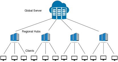
Figure 1: Server-hubs-clients FL architecture with 4 hubs and 12 clients.

Mathematically, this can be modeled by problem (1). In this situation, we care about two sources of communication cost: the server and the hubs, and between the hubs and the clients. We propose to handle this via local training (LT) between the server and the hubs, and via client sampling (CS) and compressed communication (CC) between the hubs and the clients. Algorithmically, from the server-hubs perspective, we are applying a particular variant of ProxSkip-VR to (3)–(4), where $\phi_{i}$ is the aggregate loss handles by hub $i$. This takes care of communication efficiency between the server and the hub. Note also that we need not worry about partial participation of hubs, as these are designed to be always available. However, in this situation, it is costly for hub $i$ to compute the gradient of $\phi_{i}$ as this involves communication with all the clients it handles.

4.1 Handling of client sampling (CS) and compressed communication (CC)

In order to alleviate this burden, we propose a combination of CS and CC. However, we need to be very careful about how to do this. Indeed, both CS and CC, even when applied in isolation, and without ProxSkip in the mix, can lead to a substantial slowdown in convergence. For example, one will typically lose linear convergence in the strongly convex regime. However, techniques for preserving linear convergence in the presence of CS and CC exist: this is what variance reduction strategies are designed to do. For example, LSVRG [Hofmann et al., 2015, Kovalev et al., 2020a] is a VR technique for reducing the variance due to CS, and DIANA [Mishchenko et al., 2019] is a VR technique for reducing the variance due to CC. However, we are not aware of any VR method that combines CS (applied first) and CC (applied second).

We now propose such a technique. In iteration $t$, every hub $i\in\{1,2,\dots,M\}$ selects a random subset $\mathcal{S}_{t}^{i}\subseteq\{1,2,\dots,n_{i}\}$ of the clients it handles of cardinality $\tau_{i}$, chosen uniformly at random, and estimates the hub gradient via

$$\nabla\phi_{i}(x_{t})\approx g_{t}^{i}\coloneqq\frac{1}{|\mathcal{S}_{t}^{i}|}\sum\limits_{j\in\mathcal{S}_{t}^{i}}\mathcal{Q}_{t}^{ij}\left(\nabla\phi_{ij}(x_{t})-\nabla\phi_{ij}(y_{t})\right)+\nabla\phi_{i}(y_{t}),$$ (11)

where $\mathcal{Q}_{t}^{ij}:\mathbb{R}^{d^{\prime}}\to\mathbb{R}^{d^{\prime}}$ is a randomized compression (e.g., sparsification or quantization) operator [Alistarh et al., 2017, Khirirat et al., 2018, Horváth et al., 2019b, a, Philippenko and Dieuleveut, 2020], i.e., a mapping satisfying

$$\mathbb{E}\left[Q_{t}^{ij}(x)\right]=x,\quad\mathbb{E}\left[\|Q_{t}^{ij}(x)-x\|^{2}\right]\leq\omega\left\|x\right\|^{2},\quad\forall x\in\mathbb{R}^{d^{\prime}},$$ (12)

and the control vector $y_{t}$ is updated probabilistically as follows:

$$y_{t+1}=\left\{\begin{array}[]{lll}x_{t}&\text{ with probability }&q\\ y_{t}&\text{ with probability }&1-q\end{array}\right..$$ (13)

The global gradient estimator (a vector in $\mathbb{R}^{Md^{\prime}}$), which we call HUB, is construcuted as a concatenation of the above hub estimators:

$$\nabla f(x_{t})\coloneqq\left(\frac{n_{i}}{n}\nabla\phi_{i}(x_{t})\right)_{i=1}^{M}\approx g_{t}\coloneqq g(x_{t},y_{t},\xi_{t})\coloneqq\left(\frac{n_{i}}{n}g_{t}^{i}\right)_{i=1}^{M},$$ (14)

where $\xi_{t}$ represents the combined randomness from the compressors $\{\mathcal{Q}_{t}^{ij}\}$ and random sets $\{\mathcal{S}_{t}^{i}\}$.

In order to analyze ProxSkip-VR in the consensus form, from now on we assume that $n_{i}=m=\nicefrac{{n}}{{M}}$ and $\tau_{i}=\tau\in\{1,2,\dots,m\}$ for all $i$, and rely on a slightly different, more general reformulation:

$$\min\limits_{x\in\mathbb{R}^{d}}\frac{1}{m}\sum\limits_{j=1}^{m}\widetilde{\phi}_{j}(x)+r(x),\quad\widetilde{\phi}_{j}(x)\coloneqq\frac{1}{M}\sum\limits_{i=1}^{M}\phi_{ij}\left(x_{i}\right),\quad r(x)\coloneqq\begin{cases}0&\text{ if }x_{1}=\cdots=x_{M},\\ +\infty&\text{ otherwise.}\end{cases}$$

Our proposed method ProxSkip-HUB is ProxSkip-VR combined with the novel HUB estimator (14), applied to the above reformulation; see Algorithm 2.

Algorithm 2 ProxSkip-HUB

1:  Input: stepsize $\gamma>0$, probabilities $p>0$, $q>0$, initial iterate $x_{0}\in\mathbb{R}^{d}$, initial shift ${\color[rgb]{0.75390625,0.09765625,0.09765625}y_{0}}\in\mathbb{R}^{d}$, initial control variate ${\color[rgb]{0,0,1}h_{0}}\in\mathbb{R}^{d}$, number of iterations $T\geq 1$

2:  for $t=0,1,\dotsc,T-1$ do

3:     broadcast $x_{t}$ to all clients

4:     for $i\in S_{t}$ do

5:        $\hat{\Delta}_{t}^{i}=Q\left(\nabla f_{i}(x_{t})-\nabla f_{i}({\color[rgb]{0.75390625,0.09765625,0.09765625}y_{t}})\right)$ $\diamond$ Apply compression operator

6:     end for

7:     $\hat{\Delta}_{t}=\frac{1}{\tau}\sum_{i\in S_{t}}\hat{\Delta}_{t}^{i}$

8:     $\hat{g}=\hat{\Delta}_{t}+\nabla f({\color[rgb]{0.75390625,0.09765625,0.09765625}y_{t}})$

9:     $\hat{x}_{t+1}=x_{t}-\gamma(\hat{g}_{t}-{\color[rgb]{0,0,1}h_{t}})$ $\diamond$ Take a gradient-type step adjusted via the control variate ${\color[rgb]{0.75390625,0.09765625,0.09765625}h_{t}}$

10:     Flip a coin $\theta_{t}\in\{0,1\}$ where $\mathop{\rm Prob}(\theta_{t}=1)=p$ $\diamond$ To decide whether to skip the prox or not

11:     if $\theta_{t}=1$ then

12:        $x_{t+1}=\operatorname{prox}_{\frac{\gamma}{p}\psi}\bigl{(}\hat{x}_{t+1}-\frac{\gamma}{p}{\color[rgb]{0,0,1}h_{t}}\bigr{)}$ $\diamond$ Apply prox, but only very rarely! (with probability $p$)

13:     else

14:        $x_{t+1}=\hat{x}_{t+1}$ $\diamond$ Skip the prox!

15:     end if

16:     ${\color[rgb]{0.75390625,0.09765625,0.09765625}h_{t+1}}={\color[rgb]{0.75390625,0.09765625,0.09765625}h_{t}}+\frac{p}{\gamma}(x_{t+1}-\hat{x}_{t+1})$ $\diamond$ Update the control variate ${\color[rgb]{0,0,1}h_{t}}$

17:     $y_{t+1}=\left\{\begin{array}[]{lll}x_{t}&\text{ with probability }&q\\ y_{t}&\text{ with probability }&1-q\end{array}\right.$ $\diamond$ Update the shift ${\color[rgb]{0.75390625,0.09765625,0.09765625}y_{t}}$

18:  end for

4.2 Theory for ProxSkip-HUB

In the following result we first claim that the above estimator satisfies Assumption 4 with $C=\tilde{C}=0$ (i.e., it is variance-reduced), and the rest of the claim follows by application of our general theorem Theorem 5.

Theorem 9.

Assume that $\nabla\widetilde{\phi}_{j}$ is $L_{j}$-smooth for all $j$ and let Assumptions 2 and 3 hold. Then for the gradient estimator (14), Assumption 4 holds with the following constants:

$$A=4\left(L(\tau)+\frac{\omega}{\tau}L_{\max}\right),\quad B=4\left(1+\frac{\omega}{\tau}\right),\quad C=0,\quad\tilde{A}=qL_{\max},\quad\tilde{B}=1-q,\quad\tilde{C}=0,$$

and $\sigma_{t}\coloneqq\sigma(y_{t})$, $\sigma(y)\coloneqq\frac{1}{m}\sum_{j=1}^{m}\|\nabla\widetilde{\phi}_{j}(y)-\nabla\widetilde{\phi}_{j}(x_{\star})\|^{2}$, $L_{\max}\coloneqq\max_{j}L_{j}$. Set $W=\nicefrac{{2B}}{{(1-\tilde{B})}}$ and $0<\gamma\leq\min\left\{\nicefrac{{1}}{{\mu}},\nicefrac{{1}}{{(A+W\tilde{A})}}\right\}.$ Then the iterates of ProxSkip-VR for any $p\in(0,1]$ satisfy

$$\mathbb{E}\left[\Psi_{T}\right]\leq\max\left\{(1-\gamma\mu)^{T},(1-p^{2})^{T},\left(1-\frac{q}{2}\right)^{T}\right\}\Psi_{0},$$

where the Lyapunov function is defined by

$$\Psi_{t}\coloneqq\|x_{t}-x_{\star}\|^{2}+\frac{\gamma^{2}}{p^{2}}\|h_{t}-h_{\star}\|^{2}+\gamma^{2}\frac{8}{q}\left(1+\frac{\omega}{\tau}\right)\sigma_{t}.$$

We now consider two special cases. In the first, we specialize to the no compression regime, and in the second, to the full participation regime.

Corollary 1 (No compression).

If we do not use compression (i.e., $\omega=0$), then the communication and iteration complexities are

$$\#comms=\mathcal{O}\left(\sqrt{\frac{L_{\max}}{\mu}}\log\frac{1}{\varepsilon}\right),\qquad\#iters=\mathcal{O}\left(\frac{L_{\max}}{\mu}\log\frac{1}{\varepsilon}\right),$$

respectively. However, if we use the estimator (11) in Theorem 5 directly, then the communication and iteration complexities are

$$\#comms=\mathcal{O}\left(\sqrt{\frac{L(\tau)}{\mu}}\log\frac{1}{\varepsilon}\right),\qquad\#iters=\mathcal{O}\left(\frac{L(\tau)}{\mu}\log\frac{1}{\varepsilon}\right),$$

where $L(\tau)\coloneqq\frac{m-\tau}{\tau(m-1)}L_{\max}+\frac{m(\tau-1)}{\tau(m-1)}L$.

Notice that $L_{\max}\geq L$, and that $L(\tau)=L_{\max}$ for $\tau=1$ and $L(\tau)=L$ for $\tau=m$. Moreover, $L(\tau)$ decreases as the minibatch size $\tau$ increases.

Corollary 2 (No client sampling).

If we do not use client sampling (i.e., $\tau=m$), then the communication and iteration complexities are

$$\#comms=\mathcal{O}\left(\sqrt{\frac{L_{\max}}{\mu}\left(1+\frac{\omega}{M}\right)}\log\frac{1}{\varepsilon}\right),\qquad\#iters=\mathcal{O}\left(\frac{L_{\max}}{\mu}\left(1+\frac{\omega}{M}\right)\log\frac{1}{\varepsilon}\right),$$

respectively.

Assume $r(x)\equiv 0$. If $\mathcal{Q}_{t}^{ij}(x)\equiv x$, then $\omega=0$, and we restore the well-known LSVRG method [Hofmann et al., 2015, Kovalev et al., 2020b], assuming that the functions $\phi_{ij}$ have the same smoothness constant. We can recover the same rate exactly as well, but with a slightly more refined analysis, one in which we do not need to work with compressors (LSVRG does not involve any), which makes for a tighter analysis. On the other hand, if $\tau=m$, we restore the rate of the well-known DIANA [Mishchenko et al., 2019, Horváth et al., 2019b] method and its sibling Rand-DIANA [Shulgin and Richtárik, 2021].

5 Experiments

To illustrate the predictive power of our theory, it suffices to consider $L_{2}$-regularized logistic regression in the distributed setting (1), with

$$\phi_{i}(x)=\frac{1}{n_{i}}\sum\limits_{j=1}^{n_{i}}\log\left(1+\exp\left(-b_{ij}a_{ij}^{\top}x\right)\right)+\frac{\lambda}{2}\|x\|^{2},$$

where $n_{i}$ is the number of data points per worker $a_{ij}\in\mathbb{R}^{d^{\prime}}$ and $b_{ij}\in\{-1,+1\}$ are the data samples and labels. We choose $n_{i}=m=\nicefrac{{n}}{{M}}$ for all $i$. We set the regularization parameter $\lambda=5\cdot 10^{-4}L$ by default, where $L$ is the smoothness constant of $f$. We conduct several experiments on the w8a dataset from LibSVM library [Chang and Lin, 2011].

5.1 ProxSkip-LSVRG vs baselines

In Figure 2 (first row), we compare various LT baselines for three choices of mini-batch sizes ($\tau=16,32,64$) with our method ProxSkip-VR combined with the LSVRG estimator, which is a special case of the HUB estimator when $\mathcal{Q}_{t}^{ij}(x)\equiv x$ for all $i,j$. We see that our method outperforms all other methods significantly due to its communication-acceleration properties.

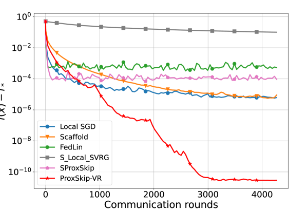
(a) $\tau=16$

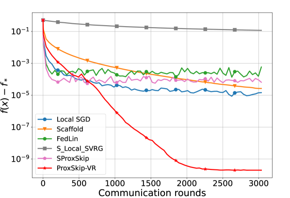
(b) $\tau=32$

(c) $\tau=64$

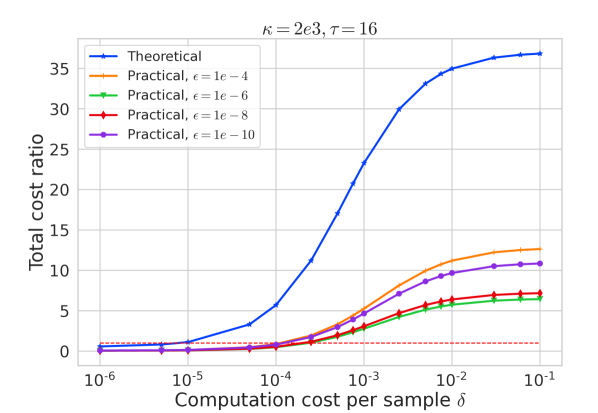
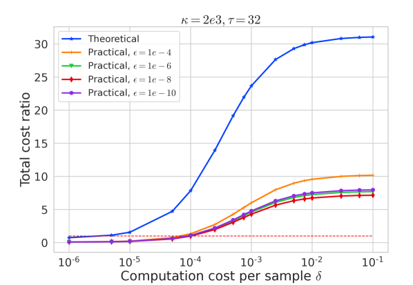
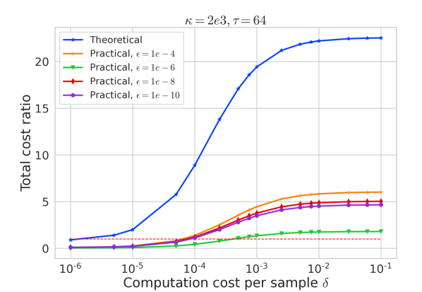
Figure 2: The top row shows the convergence results compared with baselines and the second row is the total cost ratio of ProxSkip over our ProxSkip-VR.

5.2 The total cost of ProxSkip-LSVRG can be significantly smaller than the total cost of ProxSkip, in theory and practice

Next, we derive the total cost, which includes communication cost (assumed to be $1$, for normalization purposes), and computational cost (assumed to be $\delta$; and equal to the cost of performing one SGD step with a single data point). Let us consider the total cost of ProxSkip-VR in the case of the LSVRG estimator: in each iteration we compute 1 stochastic gradient, and with probability $q$ we compute the exact gradient. We do not need to compute a second stochastic gradient since we can use memory and the relation $y_{t+1}=x_{t}$. The total cost for ProxSkip-VR is equal to

$$\text{Cost}(\text{{\sf\color[rgb]{0.75390625,0.09765625,0.09765625}ProxSkip-VR}})\coloneqq T_{\text{comm.}}(\text{{\sf\color[rgb]{0.75390625,0.09765625,0.09765625}ProxSkip-VR}})+\delta\left(qm+(1-q)\tau+\tau\right)T_{\text{iter}}({\text{{\sf\color[rgb]{0.75390625,0.09765625,0.09765625}ProxSkip-VR}}}).$$

ProxSkip requires full/exact gradient computation at each iteration, so the total cost of ProxSkip is

$$\text{Cost}(\text{{\sf\color[rgb]{0.75390625,0.09765625,0.09765625}ProxSkip}})\coloneqq T_{\text{comm.}}(\text{{\sf\color[rgb]{0.75390625,0.09765625,0.09765625}ProxSkip}})+\delta mT_{\text{iter}}({\text{{\sf\color[rgb]{0.75390625,0.09765625,0.09765625}ProxSkip}}}).$$

Using Theorems 6 and 9 and the value $L(\tau)\coloneqq\frac{m-\tau}{\tau(m-1)}L_{\max}+\frac{m(\tau-1)}{\tau(m-1)}L$ of the expected smoothness constant for sampling with minibatch size $\tau$ uniformly at random, we get the following expression for the cost ratio, expressed as a function of $\delta$:

$$\text{Cost ratio}(\delta)\coloneqq\frac{\text{Cost}(\text{{\sf\color[rgb]{0.75390625,0.09765625,0.09765625}ProxSkip}})}{\text{Cost}(\text{{\sf\color[rgb]{0.75390625,0.09765625,0.09765625}ProxSkip-VR}})}=\frac{\sqrt{\mu L}+mL\delta}{\sqrt{\mu L(\tau)}+\left(2m\mu+(2L(\tau)-2\mu)\tau\right)\delta}.$$ (15)

We can easily calculate the limits of this expression:

$$\text{Cost ratio}(\delta=0)=\sqrt{\frac{L}{L(\tau)}},\quad\quad\quad\text{Cost ratio}(\delta\to\infty)=\frac{mL}{2(m\mu+\left(L(\tau)-\mu\right)\tau)}.$$

Since $L(\tau)\geq L$, the cost ratio is below 1 when $\delta=0$ and $\tau<m$, which means that ProxSkip is better than ProxSkip-VR. This is to be expected since $\delta=0$ means that we ignore the cost of local computation entirely, which offers advantage to the former method. On the other hand, the cost ratio is an increasing function of $\delta$, and often reaches the threshold of 1 with a small value of $\delta$; in 2 (second row), this threshold is reached for $\delta\in[10^{-6},10^{-5}]$ in all three plots.

In Figure 2 (second row), we depict the theoretical cost ratio according to (15) and the corresponding experimental cost ratio obtained by an actual run of both methods to achieve $\varepsilon$-accuracy, with $\varepsilon=10^{-6}$ and $\varepsilon=10^{-8}$. Remarkably, the experimental results follows the same pattern as our theoretical prediction. The empirical curves appear lower because we use approximations for $L_{\max}$, $L$ and $\mu$. As we can see, starting from $\delta=10^{-4}$, ProxSkip-VR starts to outperform ProxSkip. As $\delta$ grows, the advantage of variance reduction embedded in ProxSkip-VR over vanilla ProxSkip grows. These results suggest that variance reduction is of practical utility in terms of the total cost, even for small values of $\delta$, and its effectiveness grows with $\delta$.

5.3 Additional experiments with ProxSkip-VR

We conduct further experiments to validate the efficiency of our proposed method ProxSkip-VR. We instantiate our variance reduction design with LSVRG and compare our method with several baselines across various datasets (w8a/a9a), different number of workers (10/20), and different batch sizes (16/32/64). All results in Figures 3, 4, 5, 6 show that ProxSkip-VR achieves linear convergence and outperforms the baselines.

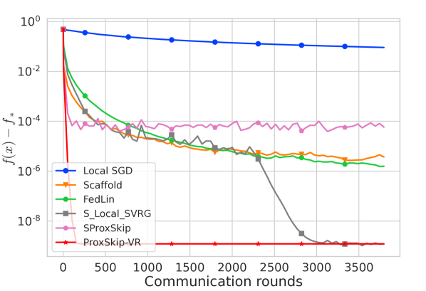
(a) $\tau=16$.

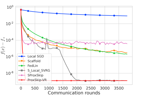
(b) $\tau=32$.

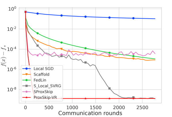
(c) $\tau=64$.

Figure 3: Convergence results with 20 distributed workers on w8a dataset, $\kappa=1e3$.

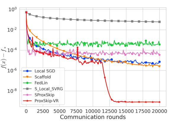
(a) $\tau=16$.

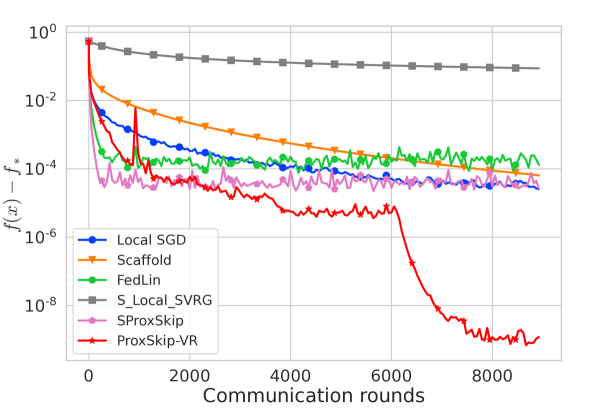
(b) $\tau=32$.

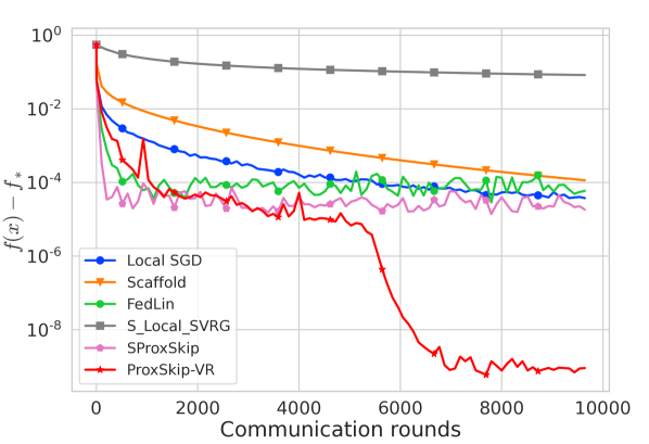
(c) $\tau=64$.

Figure 4: Convergence results with 20 distributed workers on w8a dataset, $\kappa=1e4$.

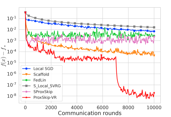
(a) $\tau=16$.

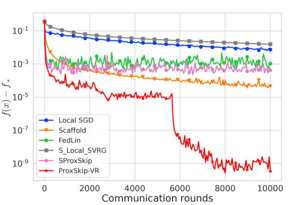
(b) $\tau=32$.

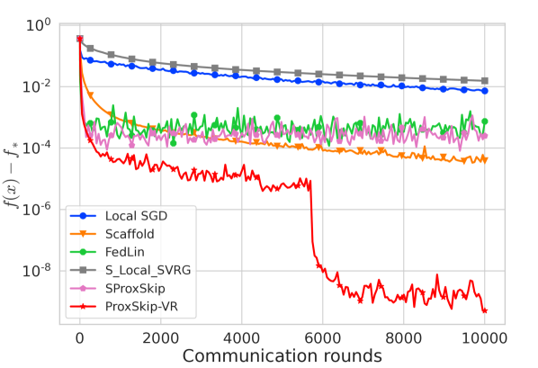
(c) $\tau=64$.

Figure 5: Convergence results with 10 distributed workers on a9a dataset, $\kappa=1e4$.

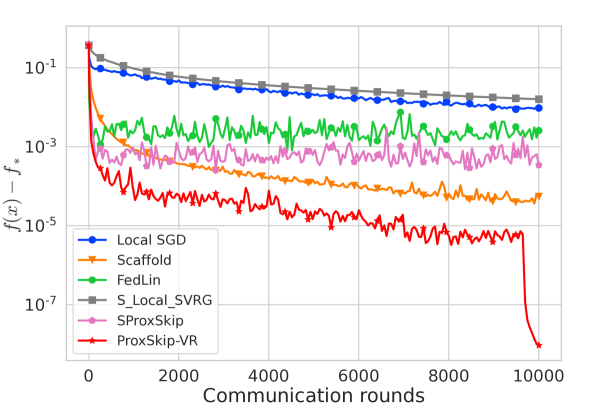
(a) $\tau=16$.

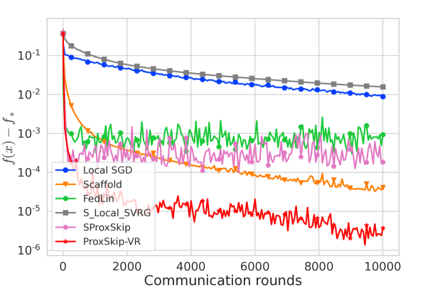
(b) $\tau=32$.

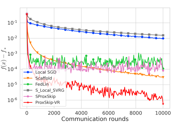
(c) $\tau=64$.

Figure 6: Convergence results with 20 distributed workers on a9a dataset, $\kappa=1e4$.

5.4 Additional experiments of cost ratio of ProxSkip over ProxSkip-VR

Here we report on more experiments related to the total cost ratio of ProxSkip over ProxSkip-VR in Figures 7, 8, 9, 10. When GD is used as the subroutine, i.e., when ProxSkip-VR reduces to ProxSkip, the ratio is equal to one, and is depicted by the red horizontal dashed line. Any cost ratio above one means that ProxSkip-VR benefits over ProxSkip (e.g., a cost ratio of $10$ means $10\times$ speedup in favor of our method). As seen in the plots, acceleration of our method over ProxSkip is clearly visible, and improves as the local computation cost $\delta$ per sample increases. For large values of $\delta$ (i.e., $\delta\approx 10^{-1}$), the acceleration can reach $20\times$ to $85\times$. Note also that acceleration is more significant for small minibatch sizes. That is, it is better for $\tau=16$ than for $\tau=32$, which is better than in the $\tau=64$ case. This means that in terms of total cost, it is beneficial for the workers to use smaller minibatch sizes, i.e., it is beneficial to be as far from the full batch regime employed by ProxSkip as possible.

(a) $\tau=16$.

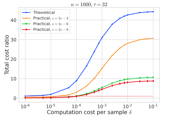
(b) $\tau=32$.

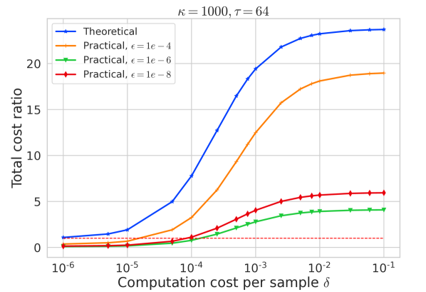
(c) $\tau=64$.

Figure 7: Acceleration with 10 distributed workers on a9a dataset, $\kappa=1e3$.

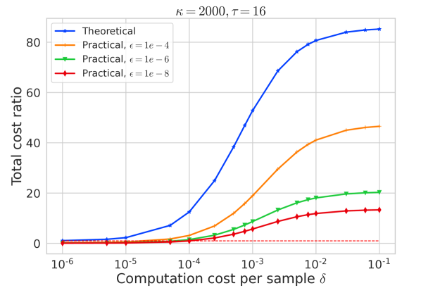
(a) $\tau=16$.

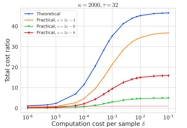
(b) $\tau=32$.

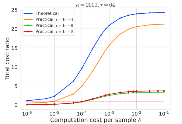
(c) $\tau=64$.

Figure 8: Acceleration with 10 distributed workers on a9a dataset, $\kappa=2e3$.

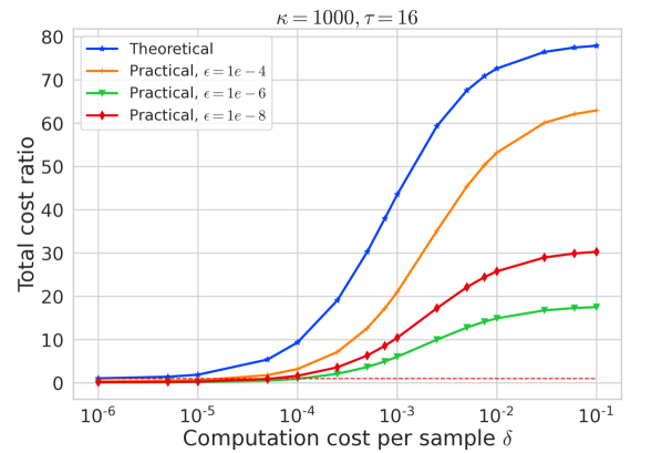
(a) $\tau=16$.

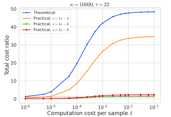
(b) $\tau=32$.

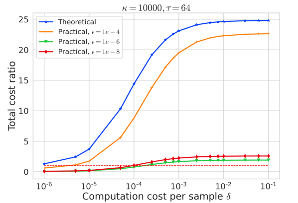
(c) $\tau=64$.

Figure 9: Acceleration with 10 distributed workers on a9a dataset, $\kappa=1e4$.

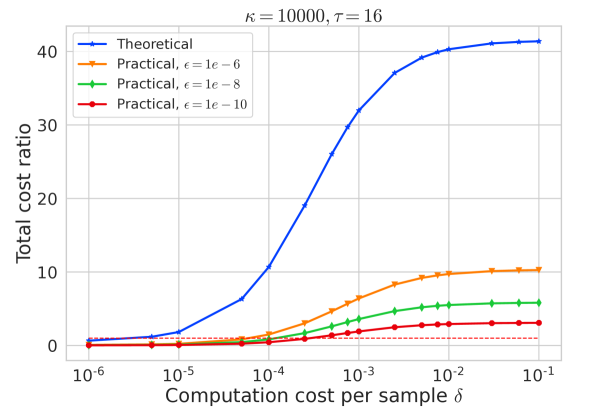
(a) $\tau=16$.

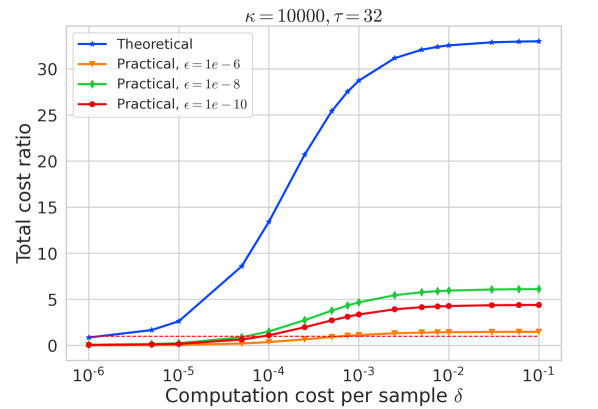
(b) $\tau=32$.

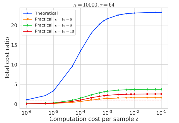
(c) $\tau=64$.

Figure 10: Acceleration with 10 distributed workers on w8a dataset, $\kappa=1e4$.

5.5 Experiments with ProxSkip-HUB

In this work we introduced a new FL architecture: regional hubs connecting the clients to the server; see Section 4. For conceptual simplicity, and in order to facilitate fair comparison with ProxSkip-LSVRG, we assume that the number of hubs equals to the number of clients, and that each client owns a single datapoint only. We compare ProxSkip-HUB with ProxSkip-LSVRG to check whether communication compression leads to any benefits in terms of total costs. Theoretically, and similarly to our analysis in Section 5, the total cost for ProxSkip-LSVRG is

$$\text{Cost}(\text{{\sf\color[rgb]{0.75390625,0.09765625,0.09765625}ProxSkip-LSVRG}})\coloneqq T_{\text{comm.}}(\text{{\sf\color[rgb]{0.75390625,0.09765625,0.09765625}ProxSkip-LSVRG}})\\ +\delta\left(qm+(1-q)\tau+\tau\right)T_{\text{iter}}({\text{{\sf\color[rgb]{0.75390625,0.09765625,0.09765625}ProxSkip-LSVRG}}}).$$

Recall that we assume the communication cost from every worker/hub to the master is equal to 1, and the computation cost per sample is equal to $\delta$. Here we generalize to the multi-level structure. We assume that the communication cost from every client to hub is equal to $\delta^{\prime}$. We choose the Rand-$k$ sparsification for ProxSkip-HUB; this compressor selects $k$-entries of the gradient vector, uniformly at random from the full $d$-dimensional gradient. The total cost of ProxSkip-HUB is

$$\text{Cost}(\text{{\sf\color[rgb]{0.75390625,0.09765625,0.09765625}ProxSkip-HUB}}) :=T_{\text{comm.}}(\text{{\sf\color[rgb]{0.75390625,0.09765625,0.09765625}ProxSkip-HUB}})$$ (16)

$$\quad+\delta^{\prime}\left(qm+\frac{k}{d}\left((1-q)\tau+\tau\right)\right)T_{\text{iter}}(\text{{\sf\color[rgb]{0.75390625,0.09765625,0.09765625}ProxSkip-HUB}}).$$

Our experimental results are summarized Figure 11; we use the values $\delta=\delta\textquoteright=10^{-2}$. Clearly, and thanks to communication compression, ProxSkip-HUB has benefit in terms of the total cost compared to ProxSkip-LSVRG, and can reach up to three degrees of magnitude!

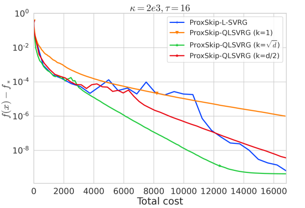
(a) $\tau=16$.

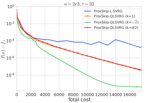
(b) $\tau=32$.

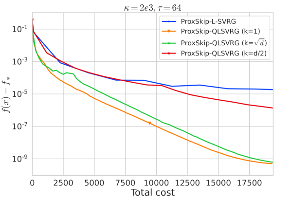
(c) $\tau=64$.

Figure 11: Convergence results with different batch sizes and sparsification parameter $k$ on a9a, $\kappa=2e3$.

Appendix

Appendix A Basic Facts

A.1 Bregman divergence, $L$-smoothness and $\mu$-strong convexity

The Bregman divergence of a differentiable function $f:\mathbb{R}^{d}\rightarrow\mathbb{R}$ is defined by

$$D_{f}(x,y):=f(x)-f(y)-\langle\nabla f(y),x-y\rangle.$$ (17)

It is easy to see that

$$\langle\nabla f(x)-\nabla f(y),x-y\rangle=D_{f}(x,y)+D_{f}(y,x),\quad\forall x,y\in\mathbb{R}^{d}.$$ (18)

For an $L$-smooth and $\mu$-strongly convex function $f:\mathbb{R}^{d}\rightarrow\mathbb{R}$, we have

$$\frac{\mu}{2}\|x-y\|^{2}\leq D_{f}(x,y)\leq\frac{L}{2}\|x-y\|^{2},\quad\forall x,y\in\mathbb{R}^{d}$$ (19)

and

$$\frac{1}{2L}\|\nabla f(x)-\nabla f(y)\|^{2}\leq D_{f}(x,y)\leq\frac{1}{2\mu}\|\nabla f(x)-\nabla f(y)\|^{2},\quad\forall x,y\in\mathbb{R}^{d}.$$ (20)

A.2 Firm-nonexpansiveness of the proximity operator

Given $\psi:\mathbb{R}^{d}\rightarrow\mathbb{R}$, we define $\psi^{*}(y):=\sup_{x\in\mathbb{R}^{d}}\{\langle x,y\rangle-\psi(x)\}$ to be its Fenchel conjugate. The proximity operator of $\psi^{*}$ satisfies for any $\tau>0$

$$\text{ if }u=\operatorname{prox}_{\tau\psi^{*}}(y),\quad\text{ then }\quad u\in y-\tau\partial\psi^{*}(u).$$ (21)

If Assumption 3 is satisfied, then firm nonexpansiveness of the proximity operator implies [Mishchenko et al., 2022] that

$$\left\|\operatorname{prox}_{\frac{\gamma}{p}\psi}(x)-\operatorname{prox}_{\frac{\gamma}{p}\psi}(y)\right\|^{2}+\left\|\left(x-\operatorname{prox}_{\frac{\gamma}{p}\psi}(x)\right)-\left(y-\operatorname{prox}_{\frac{\gamma}{p}\psi}(y)\right)\right\|^{2}\leq\|x-y\|^{2},$$ (22)

for all $x,y\in\mathbb{R}^{d}$ and any $\gamma,p>0$.

A.3 Young’s inequality

For any two vectors $a,b\in\mathbb{R}^{d}$, we have

$$\|a+b\|^{2}\leq 2\|a\|^{2}+2\|b\|^{2}.$$ (23)

A.4 Jensen’s inequality

For a convex function $h:\mathbb{R}^{d}\leftarrow\mathbb{R}$ and any vectors $x_{1},\ldots,x_{n}\in\mathbb{R}^{d}$, we have

$$h\left(\frac{1}{n}\sum_{i=1}^{n}x_{i}\right)\leq\frac{1}{n}\sum_{i=1}^{n}h\left(x_{i}\right).$$ (24)

Applying this to the squared norm, $h(x)=\|x\|^{2},$ we get

$$\left\|\frac{1}{n}\sum_{i=1}^{n}y_{i}\right\|^{2}\leq\frac{1}{n}\sum_{i=1}^{n}\left\|y_{i}\right\|^{2}.$$ (25)

Appendix B Analysis of ProxSkip-VR

In this section we provide the proof of Theorem 5.

B.1 Main lemma of ProxSkip

We start from Lemma 1 initially introduced by Mishchenko et al. [2022]; for completeness we provide the whole proof. Let us define two additional sequences:

$$\hat{w}_{t}=x_{t}-\gamma\hat{g}_{t}\left(x_{t}\right),\qquad\hat{w}_{\star}=x_{\star}-\gamma\hat{g}_{t}\left(x_{\star}\right).$$ (26)

Lemma 1.

If Assumption 3 holds, $\gamma>0$ and $0<p\leq 1$, then the iterates of ProxSkip-VR satisfy

$$\mathbb{E}\left[\|x_{t+1}-x_{\star}\|^{2}+\frac{\gamma^{2}}{p^{2}}\|h_{t+1}-h_{\star}\|^{2}\right]\leq\left\|\hat{w}_{t}-w_{\star}\right\|^{2}+\left(1-p^{2}\right)\frac{\gamma^{2}}{p^{2}}\left\|h_{t}-h_{\star}\right\|^{2}.$$ (27)

Proof.

In order to simplify, let us define two points:

$$x\coloneqq\hat{x}_{t+1}-\frac{\gamma}{p}h_{t},\quad y\coloneqq x_{\star}-\frac{\gamma}{p}h_{\star}.$$ (28)

STEP 1 (Optimality conditions).

Using the first-order optimality conditions for $f+\psi$ and using $h_{\star}\coloneqq\nabla f(x_{\star})$, we obtain the following fixed-point identity for $x_{\star}$:

$$x_{\star}=\operatorname{prox}_{\frac{\gamma}{p}\psi}\left(x_{\star}-\frac{\gamma}{p}h_{\star}\right)=\operatorname{prox}_{\frac{\gamma}{p}\psi}(y).$$ (29)

STEP 2 (Recalling the steps of the method).

Recall that the vectors $x_{t}$ and $h_{t}$ are in Algorithm 1 updated as follows:

$$x_{t+1}=\left\{\begin{array}[]{lll}\operatorname{prox}_{\frac{\gamma}{p}\psi}(x)&\text{ with probability }&p\\ \hat{x}_{t+1}&\text{ with probability }&1-p\end{array}\right.$$ (32)

and

$$h_{t+1}=h_{t}+\frac{p}{\gamma}\left(x_{t+1}-\hat{x}_{t+1}\right)=\left\{\begin{array}[]{lll}h_{t}+\frac{p}{\gamma}\left(\operatorname{prox}_{\frac{\gamma}{p}\psi}(x)-\hat{x}_{t+1}\right)&\text{ with probability }p\\ h_{t}&\text{ with probability }1-p\end{array}\right..$$ (35)

Let us consider the expected value $V_{t+1}\coloneqq\mathbb{E}\left[\left\|x_{t+1}-x_{\star}\right\|^{2}+\frac{\gamma^{2}}{p^{2}}\left\|h_{t+1}-h_{\star}\right\|^{2}\right]$:

$$V_{t+1} \stackrel{{\scriptstyle(\ref{eq:x_upd})+(\ref{eq:h_upd})}}{{=}} p\left(\left\|\operatorname{prox}_{\frac{\gamma}{p}\psi}(x)-x_{\star}\right\|^{2}+\frac{\gamma^{2}}{p^{2}}\left\|h_{t}+\frac{p}{\gamma}\left(\operatorname{prox}_{\frac{\gamma}{p}\psi}(x)-\hat{x}_{t+1}\right)-h_{\star}\right\|^{2}\right)$$ (36)

$$\quad+(1-p)\left(\left\|\hat{x}_{t+1}-x_{\star}\right\|^{2}+\frac{\gamma^{2}}{p^{2}}\left\|h_{t}-h_{\star}\right\|^{2}\right)$$

$$\stackrel{{\scriptstyle(\ref{eq:opt})}}{{=}} p\left(\left\|\operatorname{prox}_{\frac{\gamma}{p}\psi}(x)-\operatorname{prox}_{\frac{\gamma}{p}\psi}(y)\right\|^{2}+\left\|\frac{\gamma}{p}h_{t}+\operatorname{prox}_{\frac{\gamma}{p}\psi}(x)-\hat{x}_{t+1}-\frac{\gamma}{p}h_{\star}\right\|^{2}\right)$$

$$\quad+(1-p)\left(\left\|\hat{x}_{t+1}-x_{\star}\right\|^{2}+\frac{\gamma^{2}}{p^{2}}\left\|h_{t}-h_{\star}\right\|^{2}\right)$$

$$\stackrel{{\scriptstyle(\ref{eq:two_points})+(\ref{eq:opt})}}{{=}} p\left(\left\|\operatorname{prox}_{\frac{\gamma}{p}\psi}(x)-\operatorname{prox}_{\frac{\gamma}{p}\psi}(y)\right\|^{2}+\left\|\operatorname{prox}_{\frac{\gamma}{p}\psi}(x)-x+y-\operatorname{prox}_{\frac{\gamma}{p}\psi}(y)\right\|^{2}\right)$$

$$\quad+(1-p)\left(\left\|\hat{x}_{t+1}-x_{\star}\right\|^{2}+\frac{\gamma^{2}}{p^{2}}\left\|h_{t}-h_{\star}\right\|^{2}\right).$$

STEP 4 (Applying firm nonexpansiveness).

Applying firm nonexpansiveness of the proximal operator (22), this leads to the inequality

$$V_{t+1} \stackrel{{\scriptstyle\eqref{eq:9u0fd9h0fd9h}+(\ref{eq:firm-prox})}}{{\leq}} p\|x-y\|^{2}+(1-p)\left(\left\|\hat{x}_{t+1}-x_{\star}\right\|^{2}+\frac{\gamma^{2}}{p^{2}}\left\|h_{t}-h_{\star}\right\|^{2}\right)$$

$$\stackrel{{\scriptstyle(\ref{eq:two_points})}}{{=}} p\left\|\hat{x}_{t+1}-\frac{\gamma}{p}h_{t}-\left(x_{\star}-\frac{\gamma}{p}h_{\star}\right)\right\|^{2}+(1-p)\left(\left\|\hat{x}_{t+1}-x_{\star}\right\|^{2}+\frac{\gamma^{2}}{p^{2}}\left\|h_{t}-h_{\star}\right\|^{2}\right).$$

STEP 5 (Simple algebra).

Next, we expand the squared norm and collect the terms, obtaining

$$V_{t+1} \leq p\left\|\hat{x}_{t+1}-x_{\star}\right\|^{2}+p\frac{\gamma^{2}}{p^{2}}\left\|h_{t}-h_{\star}\right\|^{2}-2\gamma\left\langle\hat{x}_{t+1}-x_{\star},h_{t}-h_{\star}\right\rangle$$ (37)

$$\quad+(1-p)\left(\left\|\hat{x}_{t+1}-x_{\star}\right\|^{2}+\frac{\gamma^{2}}{p^{2}}\left\|h_{t}-h_{\star}\right\|^{2}\right)$$

$$= \left\|\hat{x}_{t+1}-x_{\star}\right\|^{2}-2\gamma\left\langle\hat{x}_{t+1}-x_{\star},h_{t}-h_{\star}\right\rangle+\frac{\gamma^{2}}{p^{2}}\left\|h_{t}-h_{\star}\right\|^{2}.$$

Finally, note that by our definition of $\hat{w}_{t}$, we have the identity $\hat{x}_{t+1}=\hat{w}_{t}+\gamma h_{t}$. Therefore, the first two terms above can be rewritten as

$$\left\|\hat{x}_{t+1}-x_{\star}\right\|^{2}-2\gamma\left\langle\hat{x}_{t+1}-x_{\star},h_{t}-h_{\star}\right\rangle =\left\|\hat{w}_{t}-w_{\star}+\gamma\left(h_{t}-h_{\star}\right)\right\|^{2}$$

$$\quad-2\gamma\left\langle\hat{w}_{t}-w_{\star}+\gamma\left(h_{t}-h_{\star}\right),h_{t}-h_{\star}\right\rangle$$

$$=\left\|\hat{w}_{t}-w_{\star}\right\|^{2}+2\gamma\left\langle\hat{w}_{t}-w_{\star},h_{t}-h_{\star}\right\rangle$$

$$\quad+\gamma^{2}\left\|h_{t}-h_{\star}\right\|^{2}-2\gamma\left\langle\hat{w}_{t}-w_{\star},h_{t}-h_{\star}\right\rangle$$

$$\quad-2\gamma^{2}\left\|h_{t}-h_{\star}\right\|^{2}$$

$$=\left\|\hat{w}_{t}-w_{\star}\right\|^{2}-\gamma^{2}\left\|h_{t}-h_{\star}\right\|^{2}.$$ (38)

Finally, plugging (B.1) into (37), we get:

$$V_{t+1}\leq\left\|\hat{w}_{t}-w_{\star}\right\|^{2}+\left(1-p^{2}\right)\frac{\gamma^{2}}{p^{2}}\left\|h_{t}-h_{\star}\right\|^{2}.$$

∎

B.2 Main lemma

This lemma allows us to obtain a useful recursion for variance-reduced stochastic estimators used in our ProxSkip-VR algorithm.

Lemma 2.

Let Assumptions 2 and 4 hold. Then the iterates of ProxSkip-VR satisfy

$$\mathbb{E}\left[\|\hat{w}_{t}-w_{\star}\|^{2}\right]\leq(1-\gamma\mu)\|x_{t}-x_{\star}\|^{2}-2\gamma D_{f}(x_{t},x_{\star})\left(1-\gamma A\right)+\gamma^{2}B\sigma_{t}+\gamma^{2}C.$$

Proof.

We start from the definitions of the auxiliary sequence $\hat{w}_{t}$ (see (26)):

$$\|\hat{w}_{t}-w_{\star}\|^{2} \overset{\eqref{eq:seqs}}{=} \|x_{t}-\gamma\hat{g}_{t}-(x_{\star}-\gamma\nabla f(x_{\star}))\|^{2}$$ (39)

$$= \|(x_{t}-x_{\star})-\gamma(\hat{g}_{t}-\nabla f(x_{\star}))\|^{2}$$

$$= \|x_{t}-x_{\star}\|^{2}-2\gamma\left\langle x_{t}-x_{\star},\hat{g}_{t}-\nabla f(x_{\star})\right\rangle+\gamma^{2}\|\hat{g}_{t}-\nabla f(x_{\star})\|^{2}.$$

Taking expectation in (39) and using unbiasedness of $\hat{g}_{t}$ (see (5) in Assumption 4), we get

$$\mathbb{E}\left[\|\hat{w}_{t}-w_{\star}\|^{2}\right]\overset{\eqref{32}+\eqref{eq:unbiased}}{=}\|x_{t}-x_{\star}\|^{2}-2\gamma\left\langle x_{t}-x_{\star},\nabla f(x_{t})-\nabla f(x_{\star})\right\rangle+\gamma^{2}\mathbb{E}\left[\|\hat{g}_{t}-\nabla f(x_{\star})\|^{2}\right].$$ (40)

Let us now consider the inner product in (40). Using (19) and (18), we obtain

$$\mathbb{E}\left[\|\hat{w}_{t}-w_{\star}\|^{2}\right]\leq(1-\gamma\mu)\|x_{t}-x_{\star}\|^{2}-2\gamma D_{f}(x_{t},x_{\star})+\gamma^{2}\mathbb{E}\left[\|\hat{g}_{t}-\nabla f(x_{\star})\|^{2}\right].$$ (41)

To bound the last term in (41), we can apply Assumption 4:

$$\mathbb{E}\left[\|\hat{g}_{t}-\nabla f(x_{\star})\|^{2}\right]\leq 2AD_{f}(x_{t},x_{\star})+B\sigma_{t}+C.$$ (42)

Plugging (42) into (41) gives us

$$\mathbb{E}\left[\|\hat{w}_{t}-w_{\star}\|^{2}\right] \leq(1-\gamma\mu)\|x_{t}-x_{\star}\|^{2}-2\gamma D_{f}(x_{t},x_{\star})+\gamma^{2}\left(2AD_{f}(x_{t},x_{\star})+B\sigma_{t}+C\right)$$

$$\leq(1-\gamma\mu)\|x_{t}-x_{\star}\|^{2}-2\gamma D_{f}(x_{t},x_{\star})\left(1-\gamma A\right)+\gamma^{2}B\sigma_{t}+\gamma^{2}C,$$ (43)

which is what we set out to prove. ∎

B.3 Proof of Theorem 5

Proof.

Using definition of the Lyapunov function $\Psi_{t}$, and the tower property of conditional expectation, we obtain

$$\mathbb{E}\left[\Psi_{t+1}\right] = \mathbb{E}\left[\|x_{t+1}-x_{\star}\|^{2}+\frac{\gamma^{2}}{p^{2}}\|h_{t+1}-h_{\star}\|^{2}+W\gamma^{2}\sigma_{t+1}\right]$$ (44)

$$\stackrel{{\scriptstyle\eqref{eq:lemma1}}}{{\leq}} \mathbb{E}\left[\|\hat{w}_{t}-w_{\star}\|^{2}\right]+(1-p^{2})\frac{\gamma^{2}}{p^{2}}\|h_{t}-h_{\star}\|^{2}$$

$$\quad+W\gamma^{2}\left(2\tilde{A}D_{f}(x_{t},x_{\star})+\tilde{B}\sigma_{t}+\tilde{C}\right)$$

$$\stackrel{{\scriptstyle\eqref{eq:le2}}}{{\leq}} (1-\gamma\mu)\|x_{t}-x_{\star}\|^{2}-2\gamma D_{f}(x_{t},x_{\star})\left(1-\gamma A\right)+\gamma^{2}B\sigma_{t}+\gamma^{2}C$$

$$\quad+(1-p^{2})\frac{\gamma^{2}}{p^{2}}\|h_{t}-h_{\star}\|^{2}+W\gamma^{2}\left(2\tilde{A}D_{f}(x_{t},x_{\star})+\tilde{B}\sigma_{t}+\tilde{C}\right)$$

$$\leq (1-\gamma\mu)\|x_{t}-x_{\star}\|^{2}-2\gamma D_{f}(x_{t},x_{\star})\left(1-\gamma(A+W\tilde{A})\right)$$

$$\quad+\gamma^{2}W\sigma_{t}\left(\frac{B+W\tilde{B}}{W}\right)+\gamma^{2}(C+W\tilde{C})+(1-p^{2})\frac{\gamma^{2}}{p^{2}}\|h_{t}-h_{\star}\|^{2}.$$

Using the stepsize bound $\gamma\leq\frac{1}{A+W\tilde{A}}$, this leads to

$$\mathbb{E}\left[\Psi_{t+1}\right] \leq(1-\gamma\mu)\|x_{t}-x_{\star}\|^{2}+\gamma^{2}W\sigma_{t}\left(\frac{B+W\tilde{B}}{W}\right)+\gamma^{2}(C+W\tilde{C})+(1-p^{2})\frac{\gamma^{2}}{p^{2}}\|h_{t}-h_{\star}\|^{2}.$$

Let us denote $\beta\coloneqq\frac{B+W\tilde{B}}{W}$. In order to obtain a contraction, we need to have $\beta<1$, which is satisfied when $W>\frac{B}{1-\tilde{B}}$, and we get

$$\mathbb{E}\left[\Psi_{t+1}\right] \leq (1-\gamma\mu)\|x_{t}-x_{\star}\|^{2}+\gamma^{2}W\sigma_{t}\beta+\gamma^{2}(C+W\tilde{C})+(1-p^{2})\frac{\gamma^{2}}{p^{2}}\|h_{t}-h_{\star}\|^{2}$$ (45)

$$\leq \max\left(1-p^{2},\beta,1-\gamma\mu\right)\Psi_{t}+\gamma^{2}(C+W\tilde{C}).$$

Finally, using the tower property of expectation and unrolling recursion (45), we get

$$\mathbb{E}\left[\Psi_{T}\right]\leq\max\left\{(1-\gamma\mu)^{T},\beta^{T},(1-p^{2})^{T}\right\}\Psi_{0}+\frac{\left(C+W\tilde{C}\right)\gamma^{2}}{\min\left\{\gamma\mu,p^{2},1-\beta\right\}}.$$

∎

Appendix C Examples of Methods Without Variance Reduction

C.1 Proof of Theorem 6 (GD estimator)

Proof.

Let us show that GD estimator $(\hat{g}_{t}=\nabla f(x_{t}))$ satisfies Assumption 4

$$\mathbb{E}\left[\|\hat{g}_{t}-\nabla f(x_{\star})\|^{2}\right]=\|\nabla f(x_{t})-\nabla f(x_{\star})\|^{2}\stackrel{{\scriptstyle\eqref{eq:smooth-norms}}}{{\leq}}2LD_{f}(x_{t},x_{\star}).$$

This means that Assumption 4 is satisfied with the following constant:

$$A=L,\quad B=0,\quad C=0,\quad\tilde{A}=0,\quad\tilde{B}=0,\quad\tilde{C}=0,\quad\sigma_{t}\equiv 0.$$

Applying Theorem 5 leads to final recursion:

$$\mathbb{E}\left[\Psi_{T}\right]\leq\max\left\{(1-\gamma\mu)^{T},(1-p^{2})^{T}\right\}\Psi_{0},$$ (46)

By inspecting (46) it is easy to see that

$$T\geq\max\left\{\frac{1}{\gamma\mu},\frac{1}{p^{2}}\right\}\log\frac{1}{\varepsilon}\qquad\Longrightarrow\qquad\mathbb{E}\left[\Psi_{T}\right]\leq\varepsilon\Psi_{0}.$$ (47)

Then the communication complexity is equal to

$$pT\geq\max\left\{\frac{p}{\gamma\mu},\frac{1}{p}\right\}\log\frac{1}{\varepsilon}.$$ (48)

Setting $\gamma=\frac{1}{L}$ and solving $\frac{pL}{\mu}=\frac{1}{p}$ gives the optimal probability

$$p=\sqrt{\frac{\mu}{L}}=\frac{1}{\sqrt{\kappa}}$$ (49)

Finally, the iteration complexity and communication complexity have the following form:

$$T \geq\max\left\{\frac{1}{\gamma\mu},\frac{1}{p^{2}}\right\}\log\frac{1}{\varepsilon}=\kappa\log\frac{1}{\varepsilon},$$ (50)

$$pT \geq\max\left\{\frac{p}{\gamma\mu},\frac{1}{p}\right\}\log\frac{1}{\varepsilon}=\sqrt{\kappa}\log\frac{1}{\varepsilon}.$$ (51)

∎

This recovers the result obtained by Mishchenko et al. [2022].

C.2 Proof of Theorem 8 (SGD estimator)

Proof.

Let us show that the SGD estimator $\hat{g}_{t}=g(x_{t},\xi_{t})$ satisfying Assumption 7 also satisfies Assumption 4. Using Young’s inequality we get

$$\mathbb{E}\left[\|\hat{g}_{t}-\nabla f(x_{\star})\|^{2}\right] = \mathbb{E}\left[\|g(x_{t},\xi_{t})-\nabla f(x_{\star})\|^{2}\right]$$ (52)

$$= \mathbb{E}\left[\|g(x_{t},\xi_{t})-g(x_{\star},\xi_{t})+g(x_{\star},\xi_{t})-\nabla f(x_{\star})\|^{2}\right]$$

$$\stackrel{{\scriptstyle\eqref{youngs}}}{{\leq}} 2\mathbb{E}\left[\|g(x_{t},\xi_{t})-g(x_{\star},\xi_{t})\|^{2}\right]+2\mathbb{E}\left[g(x_{\star},\xi_{t})-\nabla f(x_{\star})\|^{2}\right]$$

$$\stackrel{{\scriptstyle\eqref{Expected_smoothness}}}{{\leq}} 4A^{\prime\prime}D_{f}(x_{t},x_{\star})+2{\rm Var}(g(x_{\star},\xi)).$$

This means that Assumption 4 is satisfied with the following constants:

$$A=2A^{\prime\prime},\quad B=0,\quad C=2{\rm Var}(g(x_{\star},\xi)),\quad\tilde{A}=0,\quad\tilde{B}=0,\quad\tilde{C}=0,\quad\sigma_{t}\equiv 0.$$

Applying Theorem 5 leads to the final bound:

$$\mathbb{E}\left[\Psi_{T}\right]\leq\max\left\{(1-\gamma\mu)^{T},(1-p^{2})^{T}\right\}\Psi_{0}+\gamma^{2}\frac{2{\rm Var}(g(x_{\star},\xi))}{\min\left\{\gamma\mu,p^{2}\right\}}.$$ (53)

In order to minimize the number of prox evaluations, whatever the choice of $\gamma$ will be, we choose the smallest probability $p$ which does not lead to any degradation of the rate $\min\{\gamma\mu,p^{2}\}.$ That is, we choose $p=\sqrt{\gamma\mu}$. The first term on the right-hand side of (53) can be bounded as follows:

$$T\geq\frac{1}{\gamma\mu}\log\left(\frac{2\Psi_{0}}{\varepsilon}\right)\quad\Longrightarrow\quad(1-\gamma\mu)^{T}\Psi_{0}\leq\frac{\varepsilon}{2}.$$

The second term on the right-hand side of (53) can be bounded as follows:

$$\gamma\leq\frac{\varepsilon\mu}{2C}\quad\Longrightarrow\quad\frac{\gamma C}{\mu}\leq\frac{\varepsilon}{2}.$$

We choose the largest stepsize consistent with bounds $\gamma\leq\frac{\varepsilon\mu}{2C}$ and $\gamma\leq\frac{1}{A}$:

$$\gamma=\min\left\{\frac{1}{A},\frac{\varepsilon\mu}{2C}\right\}.$$

Using this stepsizem we get the following iteration and (expected) communication complexities:

$$T\geq\max\left\{\frac{A}{\mu},\frac{2C}{\varepsilon\mu^{2}}\right\}\log\left(\frac{2\Psi_{0}}{\varepsilon}\right),\qquad pT\geq\max\left\{\sqrt{\frac{A}{\mu}},\sqrt{\frac{2C}{\varepsilon\mu^{2}}}\right\}\log\left(\frac{2\Psi_{0}}{\varepsilon}\right).$$

This recovers the result obtained by Mishchenko et al. [2022]. ∎

Appendix D Analysis of ProxSkip-HUB

In this section we provide analysis of the new algorithm ProxSkip-HUB, which works for the new FL formulation described in Section 4. The pseudocode is presented in Algorithm 2.

D.1 Lemma for minibatch sampling

Fix a minibatch size $\tau\in\{1,2,\ldots,n\}$ and let $\mathcal{S}_{t}$ be a random subset of $\{1,2,\ldots,n\}$ of size $\tau$, chosen uniformly at random. Define the gradient estimator via

$$g(x)\coloneqq\frac{1}{\tau}\sum_{j\in\mathcal{S}_{t}}\nabla\widetilde{\phi}_{j}(x)$$ (54)

Lemma 3.

The gradient estimator $g(x)$ defined in (54) is unbiased. If we further assume that $n\geq 2$, $\widetilde{\phi}_{j}$ is convex and $L_{j}$-smooth for all $j$, and $f$ is $L$-smooth, then

$$\mathbb{E}\left[\|g(x_{t})-g(x_{\star})\|^{2}\right]\leq 2L(\tau)D_{f}(x_{t},x_{\star}),$$

where

$$L(\tau)\coloneqq\frac{n-\tau}{\tau(n-1)}\max_{j}L_{j}+\frac{n(\tau-1)}{\tau(n-1)}L.$$

Proof.

Let $\chi_{j}$ be the random variable defined by

$$\chi_{j}=\begin{cases}1&j\in S\\ 0&j\notin S\end{cases}.$$

It is easy to show that

$$\mathbb{E}\left[\chi_{j}\right]=\operatorname{Prob}(j\in S)=\frac{\tau}{n}.$$ (55)

Unbiasedness of $g(x)$ now follows via direct computation:

$$\mathbb{E}\left[g(x)\right] \stackrel{{\scriptstyle\eqref{nice_est}}}{{=}} \mathbb{E}\left[\frac{1}{\tau}\sum_{j\in S}\nabla\widetilde{\phi}_{j}(x)\right]=\mathbb{E}\left[\frac{1}{\tau}\sum_{j=1}^{n}\chi_{i}\nabla\widetilde{\phi}_{j}(x)\right]=\frac{1}{\tau}\sum_{j=1}^{n}\mathbb{E}\left[\chi_{i}\right]\nabla\widetilde{\phi}_{j}(x)$$

$$= \frac{1}{\tau}\sum_{j=1}^{n}\operatorname{Prob}(j\in S)\nabla\widetilde{\phi}_{j}(x)\stackrel{{\scriptstyle\eqref{prob}}}{{=}}\frac{1}{\tau}\sum_{j=1}^{n}\frac{\tau}{n}\nabla\widetilde{\phi}_{j}(x)=\nabla f(x).$$

Let us define

$$a_{j}\coloneqq\nabla\widetilde{\phi}_{j}(x)-\nabla\widetilde{\phi}_{j}(x_{\star}).$$ (56)

Let $\chi_{j,k}$ be the random variable defined by

$$\chi_{j,k}=\begin{cases}1&j\in\mathcal{S}_{t}\text{ and }k\in\mathcal{S}_{t}\\ 0&\text{ otherwise }\end{cases}.$$

Note that

$$\chi_{j,k}=\chi_{j}\chi_{k}.$$ (57)

Further, it is easy to show that

$$\mathbb{E}\left[\chi_{j,k}\right]=\operatorname{Prob}(j\in\mathcal{S}_{t},k\in\mathcal{S}_{t})=\frac{\tau(\tau-1)}{n(n-1)}.$$ (58)

Let us consider

$$\mathbb{E}\left[\|g(x_{t})-g(x_{\star})\|^{2}\right] = \mathbb{E}\left[\left\|\frac{1}{\tau}\sum_{j\in\mathcal{S}_{t}}\nabla\widetilde{\phi}_{j}(x)-\frac{1}{\tau}\sum_{j\in\mathcal{S}_{t}}\nabla\widetilde{\phi}_{j}(x_{\star})\right\|^{2}\right]$$ (59)

$$= \mathbb{E}\left[\left\|\frac{1}{\tau}\sum_{j\in\mathcal{S}_{t}}\left(\nabla\widetilde{\phi}_{j}(x)-\nabla\widetilde{\phi}_{j}(x_{\star})\right)\right\|^{2}\right]$$

$$\stackrel{{\scriptstyle\eqref{a_j}}}{{=}} \mathbb{E}\left[\left\|\frac{1}{\tau}\sum_{j\in\mathcal{S}_{t}}a_{j}\right\|^{2}\right]$$

$$= \frac{1}{\tau^{2}}\mathbb{E}\left[\left\|\sum_{j=1}^{n}\chi_{j}a_{j}\right\|^{2}\right]$$

$$= \frac{1}{\tau^{2}}\mathbb{E}\left[\sum_{j=1}^{n}\left\|\chi_{j}a_{j}\right\|^{2}+\sum_{k\neq j}\left\langle\chi_{j}a_{j},\chi_{k}a_{k}\right\rangle\right]$$

$$\stackrel{{\scriptstyle\eqref{indet}}}{{=}} \frac{1}{\tau^{2}}\mathbb{E}\left[\sum_{j=1}^{n}\left\|\chi_{j}a_{j}\right\|^{2}+\sum_{k\neq j}\chi_{j,k}\left\langle a_{j},a_{k}\right\rangle\right].$$

Using the formulas (55) and (58) we can continue:

$$\mathbb{E}\left[\|g(x_{t})-g(x_{\star})\|^{2}\right] =\frac{1}{\tau^{2}}\left(\frac{\tau}{n}\sum_{j=1}^{n}\left\|a_{j}\right\|^{2}+\frac{\tau(\tau-1)}{n(n-1)}\sum_{j\neq k}\left\langle a_{j},a_{k}\right\rangle\right)$$

$$=\frac{1}{\tau n}\sum_{j=1}^{n}\left\|a_{j}\right\|^{2}+\frac{\tau-1}{\tau n(n-1)}\sum_{j\neq k}\left\langle a_{j},a_{k}\right\rangle$$

$$=\frac{1}{\tau n}\sum_{j=1}^{n}\left\|a_{j}\right\|^{2}+\frac{\tau-1}{\tau n(n-1)}\left(\left\|\sum_{j=1}^{n}a_{j}\right\|^{2}-\sum_{j=1}^{n}\left\|a_{j}\right\|^{2}\right)$$

$$=\frac{n-\tau}{\tau(n-1)}\frac{1}{n}\sum_{j=1}^{n}\left\|a_{j}\right\|^{2}+\frac{n(\tau-1)}{\tau(n-1)}\left\|\frac{1}{n}\sum_{j=1}^{n}a_{j}\right\|^{2}.$$ (60)

Since $\widetilde{\phi}_{j}$ is convex and $L_{j}$-smooth, we know that

$$\left\|a_{j}\right\|^{2}=\left\|\nabla f_{j}(x_{t})-\nabla f_{j}(x_{\star})\right\|^{2}\leq 2L_{j}D_{\widetilde{\phi}_{j}}(x_{t},x_{\star}).$$ (61)

Since $f$ is convex and $L$-smooth, we know that

$$\left\|\frac{1}{n}\sum_{i=1}^{n}a_{i}\right\|^{2}=\|\nabla f(x_{t})-\nabla f(x_{\star})\|^{2}\leq 2LD_{f}(x_{t},x_{\star}).$$ (62)

Let us apply the bound $L_{j}\leq\max_{j}L_{j}$ and use the identity $D_{f}(x_{t},x_{\star})=\frac{1}{n}\sum_{j=1}^{n}D_{\widetilde{\phi}_{j}}(x_{t},x_{\star}):$

$$\mathbb{E}\left[\left\|\frac{1}{\tau}\sum_{j\in\mathcal{S}_{t}}\nabla\widetilde{\phi}_{j}(x)-\frac{1}{\tau}\sum_{j\in\mathcal{S}_{t}}\nabla\widetilde{\phi}_{j}(x_{\star})\right\|^{2}\right] \leq\frac{n-\tau}{\tau(n-1)}\frac{1}{n}\sum_{j=1}^{n}2L_{j}D_{\widetilde{\phi}_{j}}(x_{t},x_{\star})$$

$$\quad+\frac{n(\tau-1)}{\tau(n-1)}2LD_{f}(x_{t},x_{\star})$$

$$\leq 2\frac{n-\tau}{\tau(n-1)}\max_{j}L_{j}\frac{1}{n}\sum_{j=1}^{n}D_{f_{j}}(x_{t},x_{\star})$$

$$\quad+2\frac{n(\tau-1)}{\tau(n-1)}LD_{f}(x,y)$$

$$=2\frac{n-\tau}{\tau(n-1)}\max_{j}L_{j}D_{f}(x,y)$$

$$\quad+2\frac{n(\tau-1)}{\tau(n-1)}LD_{f}(x_{t},x_{\star})$$

$$=2\left(\frac{n-\tau}{\tau(n-1)}\max_{j}L_{j}+\frac{n(\tau-1)}{\tau(n-1)}L\right)D_{f}(x_{t},x_{\star}).$$

∎

D.2 Proof of Theorem 9

As in previous analysis we need to show that Assumption 4 is satisfied for the ProxSkip-HUB method.

Proof.

Let us consider the first inequality in Assumption 4 and show that it holds for the new gradient estimator $\hat{g}_{t}=\frac{1}{\tau}\sum_{j\in\mathcal{S}_{t}}Q(\nabla\widetilde{\phi}_{j}(x_{t})-\nabla\widetilde{\phi}_{j}(y_{t}))+\nabla f(y)$:

$$\mathbb{E}\left[\|\hat{g}_{t}-\nabla f(x_{\star})\|^{2}\right]=\mathbb{E}\left[\left\|\frac{1}{\tau}\sum_{j\in\mathcal{S}_{t}}Q(\nabla\widetilde{\phi}_{j}(x_{t})-\nabla\widetilde{\phi}_{j}(y_{t}))+\nabla f(y_{t})-\nabla f(x_{\star})\right\|^{2}\right].$$ (63)

Let $\Delta_{t}=\frac{1}{\tau}\sum_{j\in\mathcal{S}_{t}}(\nabla\widetilde{\phi}_{j}(x_{t})-\nabla\widetilde{\phi}_{j}(y_{t}))$ and $\hat{\Delta}_{t}=\frac{1}{\tau}\sum_{j\in\mathcal{S}_{t}}Q(\nabla\widetilde{\phi}_{j}(x_{t})-\nabla\widetilde{\phi}_{j}(y_{t}))$. Using smart zero $0=\Delta_{t}-\Delta_{t}$ we have

$$\mathbb{E}\left[\|\hat{g}_{t}-\nabla f(x_{\star})\|^{2}\right] = \mathbb{E}\left[\left\|\hat{\Delta}_{t}-\Delta_{t}+\Delta_{t}+\nabla f(y)-\nabla f(x_{\star})\right\|^{2}\right]$$ (64)

$$\stackrel{{\scriptstyle\eqref{youngs}}}{{\leq}} 2\mathbb{E}\left[\|\hat{\Delta}_{t}-\Delta_{t}\|^{2}\right]+2\mathbb{E}\left[\|\Delta_{t}+\nabla f(y_{t})-\nabla f(x_{\star})\|^{2}\right]$$

$$\leq 2\mathbb{E}\left[\left\|\frac{1}{\tau}\sum_{j\in\mathcal{S}_{t}}Q(\nabla\widetilde{\phi}_{j}(x_{t})-\nabla\widetilde{\phi}_{j}(y_{t}))-\frac{1}{\tau}\sum_{j\in\mathcal{S}_{t}}(\nabla\widetilde{\phi}_{j}(x_{t})-\nabla\widetilde{\phi}_{j}(y_{t}))\right\|^{2}\right]$$

$$\quad+2\mathbb{E}\left[\left\|\frac{1}{\tau}\sum_{j\in\mathcal{S}_{t}}(\nabla\widetilde{\phi}_{j}(x_{t})-\nabla\widetilde{\phi}_{j}(y_{t}))+\nabla f(y)-\nabla f(x_{\star})\right\|^{2}\right].$$

Let us consider the first term (64), let us define $\theta^{i}_{t}=Q(\nabla\widetilde{\phi}_{j}(x_{t})-\nabla\widetilde{\phi}_{j}(y_{t}))-(\nabla\widetilde{\phi}_{j}(x_{t})-\nabla\widetilde{\phi}_{j}(y_{t}))$:

$$\mathbb{E}\left[\|\hat{\Delta}_{t}-\Delta_{t}\|^{2}\right] =\mathbb{E}\left[\left\|\frac{1}{\tau}\sum_{j\in\mathcal{S}_{t}}Q(\nabla\widetilde{\phi}_{j}(x_{t})-\nabla\widetilde{\phi}_{j}(y_{t}))-(\nabla\widetilde{\phi}_{j}(x_{t})-\nabla\widetilde{\phi}_{j}(y_{t}))\right\|^{2}\right]$$

$$=\mathbb{E}\left[\left\|\frac{1}{\tau}\sum_{j\in\mathcal{S}_{t}}\theta_{t}^{i}\right\|^{2}\right]$$

$$=\mathbb{E}\left[\frac{1}{\tau^{2}}\left(\sum_{j\in\mathcal{S}_{t}}\left\|\theta_{t}^{i}\right\|^{2}+\sum_{i\neq j}\left\langle\theta_{t}^{i},\theta_{t}^{j}\right\rangle\right)\right]$$

$$=\frac{1}{\tau^{2}}\left(\sum_{j\in\mathcal{S}_{t}}\mathbb{E}\left[\left\|\theta_{t}^{i}\right\|^{2}\right]+\sum_{i\neq j}\mathbb{E}\left[\left\langle\theta_{t}^{i},\theta_{t}^{j}\right\rangle\right]\right).$$

Using independence and unbiasedness of compressors we have

$$\mathbb{E}\left[\|\hat{\Delta}_{t}-\Delta_{t}\|^{2}\right] = \frac{1}{\tau^{2}}\left(\sum_{j\in\mathcal{S}_{t}}\mathbb{E}\left[\left\|\theta_{t}^{i}\right\|^{2}\right]+\sum_{i\neq j}\mathbb{E}\left[\left\langle\theta_{t}^{i},\theta_{t}^{j}\right\rangle\right]\right)$$ (65)

$$= \frac{1}{\tau^{2}}\left(\sum_{j\in\mathcal{S}_{t}}\mathbb{E}\left[\left\|\theta_{t}^{i}\right\|^{2}\right]+\sum_{i\neq j}\left\langle\mathbb{E}\left[\theta_{t}^{i}\right],\mathbb{E}\left[\theta_{t}^{j}\right]\right\rangle\right)$$

$$= \frac{1}{\tau^{2}}\sum_{j\in\mathcal{S}_{t}}\mathbb{E}\left[\left\|\theta_{t}^{i}\right\|^{2}\right]$$

$$= \frac{1}{\tau^{2}}\sum_{j\in\mathcal{S}_{t}}\mathbb{E}\left[\|Q(\nabla\widetilde{\phi}_{j}(x_{t})-\nabla\widetilde{\phi}_{j}(y_{t}))-(\nabla\widetilde{\phi}_{j}(x_{t})-\nabla\widetilde{\phi}_{j}(y_{t}))\|^{2}\right]$$

$$\stackrel{{\scriptstyle\eqref{compress}}}{{\leq}} \frac{\omega}{\tau}\mathbb{E}\left[\frac{1}{\tau}\sum_{j\in\mathcal{S}_{t}}\|\nabla\widetilde{\phi}_{j}(x_{t})-\nabla\widetilde{\phi}_{j}(y_{t})\|^{2}\right].$$

Using Young’s inequality and expectation of client sampling we get

$$\mathbb{E}\left[\|\hat{\Delta}_{t}-\Delta_{t}\|^{2}\right] \stackrel{{\scriptstyle\eqref{youngs}}}{{\leq}}\frac{2\omega}{\tau}\mathbb{E}\left[\frac{1}{\tau}\sum_{j\in\mathcal{S}_{t}}\|\nabla\widetilde{\phi}_{j}(x_{t})-\nabla\widetilde{\phi}_{j}(x_{\star})\|^{2}\right]$$

$$\quad+\frac{2\omega}{\tau}\mathbb{E}\left[\frac{1}{\tau}\sum_{j\in\mathcal{S}_{t}}\|\nabla\widetilde{\phi}_{j}(y_{t})-\nabla\widetilde{\phi}_{j}(x_{\star})\|^{2}\right]$$

$$\stackrel{{\scriptstyle\eqref{youngs}}}{{\leq}}\frac{2\omega}{\tau}\frac{1}{n}\sum_{j=1}^{n}\|\nabla\widetilde{\phi}_{j}(x_{t})-\nabla\widetilde{\phi}_{j}(x_{\star})\|^{2}$$

$$\quad+\frac{2\omega}{\tau}\frac{1}{n}\sum_{j=1}^{n}\|\nabla\widetilde{\phi}_{j}(y_{t})-\nabla\widetilde{\phi}_{j}(x_{\star})\|^{2}$$

$$\stackrel{{\scriptstyle\eqref{eq:smooth-grad}}}{{\leq}}\frac{4\omega}{\tau}L_{\max}D_{f}(x_{t},x_{\star})+\frac{2\omega}{\tau}\frac{1}{n}\sum_{j=1}^{n}\|\nabla\widetilde{\phi}_{j}(y_{t})-\nabla\widetilde{\phi}_{j}(x_{\star})\|^{2}.$$ (66)

Let us consider the second term in (64):

$$\mathbb{E}\left[\left\|\frac{1}{\tau}\sum_{j\in\mathcal{S}_{t}}(\nabla\widetilde{\phi}_{j}(x_{t})-\nabla\widetilde{\phi}_{j}(y_{t}))+\nabla f(y)-\nabla f(x_{\star})\right\|^{2}\right]$$

$$=\mathbb{E}\left[\left\|\frac{1}{\tau}\sum_{j\in\mathcal{S}_{t}}(\nabla\widetilde{\phi}_{j}(x_{t})-\nabla\widetilde{\phi}_{j}(y_{t})+\nabla\widetilde{\phi}_{j}(x_{\star})-\nabla\widetilde{\phi}_{j}(x_{\star}))+\nabla f(y)-\nabla f(x_{\star})\right\|^{2}\right]$$

$$\stackrel{{\scriptstyle\eqref{youngs}}}{{\leq}}2\mathbb{E}\left[\left\|\frac{1}{\tau}\sum_{j\in\mathcal{S}_{t}}\nabla\widetilde{\phi}_{j}(x_{t})-\frac{1}{\tau}\sum_{j\in\mathcal{S}_{t}}\nabla\widetilde{\phi}_{j}(x_{\star})\right\|^{2}\right]$$

$$\quad+2\mathbb{E}\left[\left\|\frac{1}{\tau}\sum_{j\in\mathcal{S}_{t}}\nabla\widetilde{\phi}_{j}(x_{\star})-\frac{1}{\tau}\sum_{j\in\mathcal{S}_{t}}\nabla\widetilde{\phi}_{j}(y_{t})-\left(\nabla f(x_{\star})-\frac{1}{\tau}\sum_{j\in\mathcal{S}_{t}}\nabla\widetilde{\phi}_{j}(y_{t})\right)\right\|^{2}\right]$$

$$\leq 2\mathbb{E}\left[\left\|\frac{1}{\tau}\sum_{j\in\mathcal{S}_{t}}\nabla\widetilde{\phi}_{j}(x_{t})-\frac{1}{\tau}\sum_{j\in\mathcal{S}_{t}}\nabla\widetilde{\phi}_{j}(x_{\star})\right\|^{2}\right]+2\mathbb{E}\left[\left\|\frac{1}{\tau}\sum_{j\in\mathcal{S}_{t}}\nabla\widetilde{\phi}_{j}(y_{t})-\frac{1}{\tau}\sum_{j\in\mathcal{S}_{t}}\nabla\widetilde{\phi}_{j}(x_{\star})\right\|^{2}\right].$$ (67)

Using Lemma 3 and Jensen’s inequality (25) we have

$$\mathbb{E}\left[\left\|\frac{1}{\tau}\sum_{j\in\mathcal{S}_{t}}(\nabla\widetilde{\phi}_{j}(x_{t})-\nabla\widetilde{\phi}_{j}(y_{t}))+\nabla f(y)-\nabla f(x_{\star})\right\|^{2}\right]$$

$$\leq 2\mathbb{E}\left[\left\|\frac{1}{\tau}\sum_{j\in\mathcal{S}_{t}}\nabla\widetilde{\phi}_{j}(x_{t})-\frac{1}{\tau}\sum_{j\in\mathcal{S}_{t}}\nabla\widetilde{\phi}_{j}(x_{\star})\right\|^{2}\right]+2\mathbb{E}\left[\left\|\frac{1}{\tau}\sum_{j\in\mathcal{S}_{t}}\nabla\widetilde{\phi}_{j}(y_{t})-\frac{1}{\tau}\sum_{j\in\mathcal{S}_{t}}\nabla\widetilde{\phi}_{j}(x_{\star})\right\|^{2}\right]$$

$$\leq 4L(\tau)D_{f}(x_{t},x_{\star})+\frac{2}{n}\sum_{j=1}^{n}\left\|\nabla\widetilde{\phi}_{j}(y_{t})-\nabla\widetilde{\phi}_{j}(x_{\star})\right\|^{2}.$$ (68)

Combining two parts (D.2), (D.2) and plugging into (64) we get

$$\mathbb{E}\left[\|\hat{g}_{t}-\nabla f(x_{\star})\|^{2}\right] \leq 2\mathbb{E}\left[\left\|\frac{1}{\tau}\sum_{j\in\mathcal{S}_{t}}Q(\nabla\widetilde{\phi}_{j}(x_{t})-\nabla\widetilde{\phi}_{j}(y_{t}))-\frac{1}{\tau}\sum_{j\in\mathcal{S}_{t}}(\nabla\widetilde{\phi}_{j}(x_{t})-\nabla\widetilde{\phi}_{j}(y_{t}))\right\|^{2}\right]$$

$$\quad+2\mathbb{E}\left[\left\|\frac{1}{\tau}\sum_{j\in\mathcal{S}_{t}}(\nabla\widetilde{\phi}_{j}(x_{t})-\nabla\widetilde{\phi}_{j}(y_{t}))+\nabla f(y)-\nabla f(x_{\star})\right\|^{2}\right]$$

$$\leq 8L(\tau)D_{f}(x_{t},x_{\star})+\frac{4}{n}\sum_{j=1}^{n}\left\|\nabla\widetilde{\phi}_{j}(y_{t})-\nabla\widetilde{\phi}_{j}(x_{\star})\right\|^{2}$$

$$\quad+\frac{8\omega}{\tau}L_{\max}D_{f}(x_{t},x_{\star})+\frac{4\omega}{\tau}\frac{1}{n}\sum_{j=1}^{n}\|\nabla\widetilde{\phi}_{j}(y_{t})-\nabla\widetilde{\phi}_{j}(x_{\star})\|^{2}$$

$$\leq 2\cdot 4\left(L(\tau)+\frac{\omega}{\tau}L_{\max}\right)D_{f}(x_{t},x_{\star})+4\left(1+\frac{\omega}{\tau}\right)\sigma_{t},$$ (69)

where $\sigma_{t}=\frac{1}{n}\sum_{j=1}^{n}\|\nabla\widetilde{\phi}_{j}(y_{t})-\nabla\widetilde{\phi}_{j}(x_{\star})\|^{2}$. Let us consider update of control variable $y_{t}$:

$$y_{t+1}=\left\{\begin{array}[]{lll}x_{t}&\text{ with probability }&q\\ y_{t}&\text{ with probability }&1-q\end{array}\right..$$ (72)

Let us show that second inequality in Assumption 4:

$$\mathbb{E}\left[\sigma_{t+1}\right] =\mathbb{E}\left[\frac{1}{n}\sum_{j=1}^{n}\|\nabla\widetilde{\phi}_{j}(y_{t+1})-\nabla\widetilde{\phi}_{j}(x_{\star})\|^{2}\right]$$

$$=\left(1-q\right)\frac{1}{n}\sum_{j=1}^{n}\|\nabla\widetilde{\phi}_{j}(y_{t})-\nabla\widetilde{\phi}_{j}(x_{\star})\|^{2}+q\frac{1}{n}\sum_{j=1}^{n}\|\nabla\widetilde{\phi}_{j}(x_{t})-\nabla\widetilde{\phi}_{j}(x_{\star})\|^{2}$$

$$=\left(1-q\right)\sigma_{t}+2qL_{\max}D_{f}(x_{t},x_{\star}).$$ (73)

Using (D.2) and (E) bounds we can confirm that Assumption 4 is satisfied with the following constants:

$$A=4\left(L(\tau)+\frac{\omega}{\tau}L_{\max}\right),\quad B=4\left(1+\frac{\omega}{\tau}\right),\quad C=0,\quad\tilde{A}=qL_{\max},\quad\tilde{B}=1-q,\quad\tilde{C}=0.$$

Applying Theorem 5 leads to the final result

$$\mathbb{E}\left[\Psi_{T}\right]\leq\max\left\{(1-\gamma\mu)^{T},(1-p^{2})^{T},\left(1-\nicefrac{{q}}{{2}}\right)^{T}\right\}\Psi_{0},$$ (74)

where the Lyapunov function is defined by

$$\Psi_{t}\coloneqq\|x_{t}-x_{\star}\|^{2}+\frac{\gamma^{2}}{p^{2}}\|h_{t}-h_{\star}\|^{2}+\gamma^{2}\frac{8}{q}\left(1+\frac{\omega}{\tau}\right)\sigma_{t}.$$

Let us set $\gamma=\frac{1}{A+W\tilde{A}}$, $p=\sqrt{\gamma\mu}$ and $q=2\gamma\mu$. Using the same proof as for ProxSkip in Section C.1 and $L(\tau)\leq L_{\max}$ we get communication and iteration complexities:

$$T_{\text{comm.}}=\mathcal{O}\left(\sqrt{\frac{L_{\max}}{\mu}\left(1+\frac{\omega}{\tau}\right)}\log\frac{1}{\varepsilon}\right),\qquad T_{\text{iter.}}=\mathcal{O}\left(\frac{L_{\max}}{\mu}\left(1+\frac{\omega}{\tau}\right)\log\frac{1}{\varepsilon}\right).$$

∎

If we use full participation $\tau=n$ and $q=\frac{1}{\omega+1}$ and $r(x)\equiv 0$ then we get the same rate as for DIANA [Mishchenko et al., 2019, Horváth et al., 2019b] and RAND-DIANA [Shulgin and Richtárik, 2021].

Appendix E Analysis of ProxSkip-LSVRG

The analysis of ProxSkip-LSVRG is almost the same to the analysis of ProxSkip-HUB, with one exception. We use a different sigma component:

$$\sigma_{t}=\mathbb{E}\left[\left\|\frac{1}{\tau}\sum_{j\in\mathcal{S}_{t}}(\nabla\widetilde{\phi}_{j}(y_{t})-\nabla\widetilde{\phi}_{j}(x_{\star}))\right\|^{2}\right].$$ (75)

Let us consider $\mathbb{E}\left[\|\hat{g}_{t}-\nabla f(x_{\star})\|^{2}\right]$:

$$\mathbb{E}\left[\|\hat{g}_{t}-\nabla f(x_{\star})\|^{2}\right]=\mathbb{E}\left[\left\|\frac{1}{\tau}\sum_{j\in S_{t}}\left(\nabla\widetilde{\phi}_{j}(x_{t})-\nabla\widetilde{\phi}_{j}(y_{t})\right)+\nabla f(y)-\nabla f(x_{\star})\right\|^{2}\right]$$ (76)

Using (D.2) we have

$$\mathbb{E}\left[\|\hat{g}_{t}-\nabla f(x_{\star})\|^{2}\right] \leq 2\mathbb{E}\left[\left\|\frac{1}{\tau}\sum_{j\in\mathcal{S}_{t}}\nabla\widetilde{\phi}_{j}(x_{t})-\frac{1}{\tau}\sum_{j\in\mathcal{S}_{t}}\nabla\widetilde{\phi}_{j}(x_{\star})\right\|^{2}\right]$$

$$+2\mathbb{E}\left[\left\|\frac{1}{\tau}\sum_{j\in\mathcal{S}_{t}}\nabla\widetilde{\phi}_{j}(y_{t})-\frac{1}{\tau}\sum_{j\in\mathcal{S}_{t}}\nabla\widetilde{\phi}_{j}(x_{\star})\right\|^{2}\right]$$

$$\leq 4L(\tau)D_{f}(x_{t},x_{\star})+2\sigma_{t}.$$ (77)

Let us show that second inequality in Assumption 4, using Lemma 3 we get

$$\mathbb{E}\left[\sigma_{t+1}\right] =\mathbb{E}\left[\left\|\frac{1}{\tau}\sum_{j\in\mathcal{S}_{t}}(\nabla\widetilde{\phi}_{j}(y_{t+1})-\nabla\widetilde{\phi}_{j}(x_{\star}))\right\|^{2}\right]$$

$$=\left(1-q\right)\mathbb{E}\left[\left\|\frac{1}{\tau}\sum_{j\in\mathcal{S}_{t}}(\nabla\widetilde{\phi}_{j}(y_{t})-\nabla\widetilde{\phi}_{j}(x_{\star}))\right\|^{2}\right]+q\mathbb{E}\left[\left\|\frac{1}{\tau}\sum_{j\in\mathcal{S}_{t}}(\nabla\widetilde{\phi}_{j}(x_{t})-\nabla\widetilde{\phi}_{j}(x_{\star}))\right\|^{2}\right]$$

$$=\left(1-q\right)\sigma_{t}+2qL(\tau)D_{f}(x_{t},x_{\star}).$$ (78)

We showed that Assumption 4 is satisfied with following constants:

$$A=2L(\tau),\quad B=2,\quad C=0,\quad\tilde{A}=qL(\tau),\quad\tilde{B}=1-q,\quad\tilde{C}=0.$$ (79)

Applying Theorem 5 with $\gamma=\frac{1}{6L(\tau)}$ we get final bound:

$$\mathbb{E}\left[\Psi_{T}\right]\leq\max\left\{(1-\gamma\mu)^{T},(1-p^{2})^{T},\left(1-\frac{q}{2}\right)^{T}\right\}\Psi_{0},$$

where the Lyapunov function is defined as

$$\Psi_{t}\coloneqq\|x_{t}-x_{\star}\|^{2}+\frac{\gamma^{2}}{p^{2}}\|h_{t}-h_{\star}\|^{2}+\gamma^{2}\frac{4}{q}\sigma_{t}.$$

Using the same argument as for ProxSkip and setting $\frac{q}{2}=\gamma\mu$, we get

$$T_{\text{comms}}=\mathcal{O}\left(\sqrt{\frac{L(\tau)}{\mu}}\log\frac{1}{\varepsilon}\right),\qquad T_{\text{iters}}=\mathcal{O}\left(\frac{L(\tau)}{\mu}\log\frac{1}{\varepsilon}\right).$$ (80)

If $r(x)\equiv 0$, this recovers results of Kovalev et al. [2020a].

References

- Alistarh et al. [2017] D. Alistarh, D. Grubic, J. Li, R. Tomioka, and M. Vojnovic. QSGD: Communication-efficient SGD via gradient quantization and encoding. In Advances in Neural Information Processing Systems, pages 1709–1720, 2017.
- Beck [2017] A. Beck. First order methods in optimization. MOS-SIAM Series on Optimization, 2017.
- Bonawitz et al. [2017] K. Bonawitz, V. Ivanov, B. Kreuter, A. Marcedone, H. B. McMahan, S. Patel, D. Ramage, A. Segal, and K. Seth. Practical secure aggregation for privacy-preserving machine learning. In Proceedings of the 2017 ACM SIGSAC Conference on Computer and Communications Security, pages 1175–1191, 2017.
- Chang and Lin [2011] C.-C. Chang and C.-J. Lin. LibSVM: A library for support vector machines. ACM Transactions on Intelligent Systems and Technology (TIST), 2(3):27, 2011.
- Charles et al. [2021] Z. Charles, Z. Garrett, Z. Huo, S. Shmulyian, and V. Smith. On large-cohort training for federated learning. arXiv preprint arXiv:2106.07820, 2021.
- Chen et al. [2020] W. Chen, S. Horváth, and P. Richtárik. Optimal client sampling for federated learning. Privacy Preserving Machine Learning (NeurIPS 2020 Workshop), 2020.
- Cho et al. [2020] Y. J. Cho, J. Wang, and G. Joshi. Client selection in federated learning: Convergence analysis and power-of-choice selection strategies. arXiv preprint arXiv:2010.01243, 2020.
- Csiba and Richtárik [2018] D. Csiba and P. Richtárik. Importance sampling for minibatches. Journal of Machine Learning Research, 19(27):1–21, 2018.
- Defazio et al. [2014] A. Defazio, F. Bach, and S. Lacoste-Julien. SAGA: A fast incremental gradient method with support for non-strongly convex composite objectives. In Advances in Neural Information Processing Systems 27, 2014.
- Eichner et al. [2019] H. Eichner, T. Koren, H. B. McMahan, N. Srebro, and K. Talwar. Semi-cyclic stochastic gradient descent. In International Conference on Machine Learning, 2019.
- Glasgow et al. [2022] M. R. Glasgow, H. Yuan, and T. Ma. Sharp bounds for federated averaging (local sgd) and continuous perspective. In International Conference on Artificial Intelligence and Statistics, pages 9050–9090. PMLR, 2022.
- Gorbunov et al. [2020a] E. Gorbunov, F. Hanzely, and P. Richtárik. Local SGD: unified theory and new efficient methods. In NeurIPS, 2020a.
- Gorbunov et al. [2020b] E. Gorbunov, F. Hanzely, and P. Richtárik. A unified theory of SGD: Variance reduction, sampling, quantization and coordinate descent. In International Conference on Artificial Intelligence and Statistics, pages 680–690. PMLR, 2020b.
- Gorbunov et al. [2020c] E. Gorbunov, D. Kovalev, D. Makarenko, and P. Richtárik. Linearly converging error compensated SGD. Advances in Neural Information Processing Systems, 33:20889–20900, 2020c.
- Gower et al. [2019a] R. M. Gower, N. Loizou, X. Qian, A. Sailanbayev, E. Shulgin, and P. Richtárik. SGD: General analysis and improved rates. In K. Chaudhuri and R. Salakhutdinov, editors, Proceedings of the 36th International Conference on Machine Learning, volume 97 of Proceedings of Machine Learning Research, pages 5200–5209, Long Beach, California, USA, 09–15 Jun 2019a. PMLR. URL http://proceedings.mlr.press/v97/qian19b.html.
- Gower et al. [2019b] R. M. Gower, N. Loizou, X. Qian, A. Sailanbayev, E. Shulgin, and P. Richtárik. Sgd: General analysis and improved rates. In International Conference on Machine Learning, pages 5200–5209. PMLR, 2019b.
- Haddadpour and Mahdavi [2019] F. Haddadpour and M. Mahdavi. On the convergence of local descent methods infederated learning. arXiv preprint arXiv:1910.14425, 2019.
- Hofmann et al. [2015] T. Hofmann, A. Lucchi, S. Lacoste-Julien, and B. McWilliams. Variance reduced stochastic gradient descent with neighbors. Advances in Neural Information Processing Systems, 28, 2015.
- Horváth and Richtárik [2019] S. Horváth and P. Richtárik. Nonconvex variance reduced optimization with arbitrary sampling. In K. Chaudhuri and R. Salakhutdinov, editors, Proceedings of the 36th International Conference on Machine Learning, volume 97 of Proceedings of Machine Learning Research, pages 2781–2789, Long Beach, California, USA, 09–15 Jun 2019. PMLR. URL http://proceedings.mlr.press/v97/horvath19a.html.
- Horváth et al. [2019a] S. Horváth, C.-Y. Ho, Ľudovít Horváth, A. N. Sahu, M. Canini, and P. Richtárik. Natural compression for distributed deep learning. arXiv preprint arXiv:1905.10988, 2019a.
- Horváth et al. [2019b] S. Horváth, D. Kovalev, K. Mishchenko, S. Stich, and P. Richtárik. Stochastic distributed learning with gradient quantization and variance reduction. arXiv preprint arXiv:1904.05115, 2019b.
- Johnson and Zhang [2013] R. Johnson and T. Zhang. Accelerating stochastic gradient descent using predictive variance reduction. In Advances in Neural Information Processing Systems 26, pages 315–323, 2013.
- Kairouz et al. [2019] P. Kairouz, H. B. McMahan, B. Avent, A. Bellet, M. Bennis, A. N. Bhagoji, K. Bonawitz, Z. Charles, G. Cormode, R. Cummings, R. G. D’Oliveira, H. Eichner, S. E. Rouayheb, D. Evans, J. Gardner, Z. Garrett, A. Gascón, B. Ghazi, P. B. Gibbons, M. Gruteser, Z. Harchaoui, C. He, L. He, Z. Huo, B. Hutchinson, J. Hsu, M. Jaggi, T. Javidi, G. Joshi, M. Khodak, J. Konečný, A. Korolova, F. Koushanfar, S. Koyejo, T. Lepoint, Y. Liu, P. Mittal, M. Mohri, R. Nock, A. Özgür, R. Pagh, M. Raykova, H. Qi, D. Ramage, R. Raskar, D. Song, W. Song, S. U. Stich, Z. Sun, A. T. Suresh, F. Tramèr, P. Vepakomma, J. Wang, L. Xiong, Z. Xu, Q. Yang, F. X. Yu, H. Yu, and S. Zhao. Advances and open problems in federated learning. Foundations and Trends®in Machine Learning, 14(1–2):1–210, 2019.
- Karimireddy et al. [2020] S. Karimireddy, S. Kale, M. Mohri, S. Reddi, S. Stich, and A. Suresh. SCAFFOLD: Stochastic controlled averaging for on-device federated learning. In ICML, 2020.
- Khaled and Richtárik [2020] A. Khaled and P. Richtárik. Better theory for SGD in the nonconvex world. arXiv Preprint arXiv:2002.03329, 2020.
- Khaled et al. [2019] A. Khaled, K. Mishchenko, and P. Richtárik. First analysis of local GD on heterogeneous data. In NeurIPS Workshop on Federated Learning for Data Privacy and Confidentiality, pages 1–11, 2019.
- Khaled et al. [2020] A. Khaled, K. Mishchenko, and P. Richtárik. Tighter theory for local SGD on identical and heterogeneous data. In The 23rd International Conference on Artificial Intelligence and Statistics (AISTATS 2020), 2020.
- Khirirat et al. [2018] S. Khirirat, H. R. Feyzmahdavian, and M. Johansson. Distributed learning with compressed gradients. arXiv preprint arXiv:1806.06573, 2018.
- Konečný et al. [2016a] J. Konečný, H. B. McMahan, D. Ramage, and P. Richtárik. Federated optimization: distributed machine learning for on-device intelligence. arXiv:1610.02527, 2016a.
- Konečný et al. [2016b] J. Konečný, H. B. McMahan, F. Yu, P. Richtárik, A. T. Suresh, and D. Bacon. Federated learning: strategies for improving communication efficiency. In NIPS Private Multi-Party Machine Learning Workshop, 2016b.
- Kovalev et al. [2020a] D. Kovalev, S. Horváth, and P. Richtárik. Don’t jump through hoops and remove those loops: SVRG and Katyusha are better without the outer loop. In Proceedings of the 31st International Conference on Algorithmic Learning Theory, 2020a.
- Kovalev et al. [2020b] D. Kovalev, S. Horváth, and P. Richtárik. Don’t jump through hoops and remove those loops: Svrg and katyusha are better without the outer loop. In Algorithmic Learning Theory, pages 451–467. PMLR, 2020b.
- Li et al. [2014] M. Li, T. Zhang, Y. Chen, and A. J. Smola. Efficient mini-batch training for stochastic optimization. In Proceedings of the 20th ACM SIGKDD International Conference on Knowledge Discovery and Data Mining, KDD ’14, pages 661–670, New York, NY, USA, 2014. ACM. ISBN 978-1-4503-2956-9. doi: 10.1145/2623330.2623612. URL http://doi.acm.org/10.1145/2623330.2623612.
- Li et al. [2020a] T. Li, A. K. Sahu, A. Talwalkar, and V. Smith. Federated learning: challenges, methods, and future directions. IEEE Signal Processing Magazine, 37(3):50–60, 2020a. doi: 10.1109/MSP.2020.2975749.
- Li et al. [2019] X. Li, W. Yang, S. Wang, and Z. Zhang. Communication-efficient local decentralized SGD methods. arXiv preprint arXiv:1910.09126, 2019.
- Li et al. [2020b] X. Li, K. Huang, W. Yang, S. Wang, and Z. Zhang. On the conver-gence of FedAvg on non-IID data. In International Conference on Learning Representations, 2020b.
- Malinovsky et al. [2020] G. Malinovsky, D. Kovalev, E. Gasanov, L. Condat, and P. Richtárik. From local SGD to local fixed point methods for federated learning. In International Conference on Machine Learning, 2020.
- McMahan and Ramage [2017] B. McMahan and D. Ramage. Federated learning: Collaborative machine learning without centralized training data. GoogleAIBlog, Apr. 2017.
- McMahan et al. [2017] H. B. McMahan, E. Moore, D. Ramage, S. Hampson, and B. Agüera y Arcas. Communication-efficient learning of deep networks from decentralized data. In Proceedings of the 20th International Conference on Artificial Intelligence and Statistics (AISTATS), 2017.
- Mishchenko et al. [2019] K. Mishchenko, E. Gorbunov, M. Takáč, and P. Richtárik. Distributed learning with compressed gradient differences. arXiv preprint arXiv:1901.09269, 2019.
- Mishchenko et al. [2022] K. Mishchenko, G. Malinovsky, S. Stich, and P. Richtárik. ProxSkip: Yes! Local gradient steps provably lead to communication acceleration! Finally! arXiv preprint arXiv:2202.09357, 2022.
- Mitra et al. [2021] A. Mitra, R. Jaafar, G. Pappas, and H. Hassani. Linear convergence in federated learning: Tackling client heterogeneity and sparse gradients. In Advances in Neural Information Processing Systems 34, 2021.
- Moritz et al. [2016] P. Moritz, R. Nishihara, I. Stoica, and M. I. Jordan. SparkNet: Training deep networks in Spark. In International Conference on Learning Representations (ICLR), 2016.
- Nesterov [2004] Y. Nesterov. Introductory lectures on convex optimization: a basic course (Applied Optimization). Kluwer Academic Publishers, 2004.
- Nesterov [2013] Y. Nesterov. Gradient methods for minimizing composite functions. Mathematical Programming, 140(1):125–161, 2013.
- Philippenko and Dieuleveut [2020] C. Philippenko and A. Dieuleveut. Bidirectional compression in heterogeneous settings for distributed or federated learning with partial participation: tight convergence guarantees. arXiv preprint arXiv:2006.14591, 2020.
- Povey et al. [2015] D. Povey, X. Zhang, and S. Khudanpur. Parallel training of DNNs with natural gradient and parameter averaging. In ICLR Workshop, 2015.
- Shulgin and Richtárik [2021] E. Shulgin and P. Richtárik. Shifted compression framework: Generalizations and improvements. In OPT2021: 13th Annual Workshop on Optimization for Machine Learning, 2021.
- Takáč et al. [2013] M. Takáč, A. Bijral, P. Richtárik, and N. Srebro. Mini-batch primal and dual methods for SVMs. In 30th International Conference on Machine Learning, pages 537–552, 2013.
- Wang et al. [2021] J. Wang, Z. Charles, Z. Xu, G. Joshi, H. B. McMahan, B. A. y Arcas, M. Al-Shedivat, G. Andrew, S. Avestimehr, K. Daly, D. Data, S. Diggavi, H. Eichner, A. Gadhikar, Z. Garrett, A. M. Girgis, F. Hanzely, A. Hard, C. He, S. Horvath, Z. Huo, A. Ingerman, M. Jaggi, T. Javidi, P. Kairouz, S. Kale, S. P. Karimireddy, J. Konecny, S. Koyejo, T. Li, L. Liu, M. Mohri, H. Qi, S. J. Reddi, P. Richtárik, K. Singhal, V. Smith, M. Soltanolkotabi, W. Song, A. T. Suresh, S. U. Stich, A. Talwalkar, H. Wang, B. worth, S. Wu, F. X. Yu, H. Yuan, M. Zaheer, M. Zhang, T. Zhang, C. Zheng, C. Zhu, and W. Zhu. A field guide to federated optimization. arXiv preprint arXiv:2107.06917, 2021.
- Woodworth et al. [2020] B. E. Woodworth, K. K. Patel, and N. Srebro. Minibatch vs local sgd for heterogeneous distributed learning. Advances in Neural Information Processing Systems, 33:6281–6292, 2020.
- Yu et al. [2019] H. Yu, R. Jin, and S. Yang. On the linear speedup analysis of communication efficient momentum SGD for distributed non-convex optimization. In International Conference on Machine Learning (ICML), 2019.