Snipper: A Spatiotemporal Transformer for Simultaneous Multi-Person 3D Pose Estimation Tracking and Forecasting on a Video Snippet

Abstract

Multi-person pose understanding from RGB videos involves three complex tasks: pose estimation, tracking and motion forecasting. Intuitively, accurate multi-person pose estimation facilitates robust tracking, and robust tracking builds crucial history for correct motion forecasting. Most existing works either focus on a single task or employ multi-stage approaches to solving multiple tasks separately, which tends to make sub-optimal decision at each stage and also fail to exploit correlations among the three tasks. In this paper, we propose Snipper, a unified framework to perform multi-person 3D pose estimation, tracking, and motion forecasting simultaneously in a single stage. We propose an efficient yet powerful deformable attention mechanism to aggregate spatiotemporal information from the video snippet. Building upon this deformable attention, a video transformer is learned to encode the spatiotemporal features from the multi-frame snippet and to decode informative pose features for multi-person pose queries. Finally, these pose queries are regressed to predict multi-person pose trajectories and future motions in a single shot. In the experiments, we show the effectiveness of Snipper on three challenging public datasets where our generic model rivals specialized state-of-art baselines for pose estimation, tracking, and forecasting. Code is available at https://github.com/JimmyZou/Snipper.

I Introduction

Multi-person 3D pose understanding from RGB videos is a fundamental topic in computer vision, which mainly involves three complex tasks, namely multi-person pose estimation, tracking, and motion forecasting. These three tasks are all desired in a wide range of applications such as human action recognition and behavior analysis, pedestrian tracking, re-identification, human-computer interaction, and video surveillance [1, 2, 3, 4]. As an example of human behavior analysis in a crowded scene, multi-person pose estimation and tracking usually provides critical information for the accurate analysis, and motion forecasting further helps behavior forecasting and directs region-of-interest in the future for the system.

Earlier works either focus on a single task [5, 6, 7, 8, 2, 9, 10, 11, 12, 13], or employ multi-stage approaches to solving multiple tasks separately [14, 15, 16, 17, 18]. However, for the challenging scenarios with heavy occlusions, such as the example in Fig. 1, the existing methods tend to fail in correct pose estimation and robust tracking of the occluded persons in a video, and further lead to inaccurate motion forecasting due to the misleading history information. This failure can be mainly attributed to three factors: i) temporal information is not considered in the single-task methods, especially for single-frame based multi-person pose estimation [5, 6, 8, 7, 10]; ii) multi-stage methods tend to make sub-optimal decisions when addressing the three tasks step by step, because the reasoning is usually not conducted in a joint space, such as earlier works [19, 20, 21, 18] generally treat pose tracking as separate modules for the motion forecasting; and iii) the correlations among the three tasks are not fully exploited. Intuitively, accurately estimated multi-person poses facilitate robust tracking. Conversely, robust tracking provides informative region-of-interest context for the multi-person pose estimation, and it also builds the crucial history that enables sensible prediction of motion in the future.

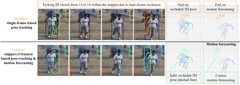
Figure 1: A practical yet challenging example to track human pose and motion forecasting. The baseline method typically adopts a tracking-by-detection schema based on single-frame inference, which fails under heavy occlusions. The proposed method Snipper resolves the ambiguity by processing video snippets with a single-stage framework instead. With the proposed attention module, Snipper aggregates spatiotemporal features shared by the three tasks. On a test set from JTA dataset with 11K 4-frame snippets that present inter-frame occlusion, Snipper obtains 84.2 3D-PCK and 62.3 MOTA (4-frame snippet) versus 80.1 3D-PCK and 59.5 MOTA (single-frame).

To address the above limitations, we propose Snipper, a unified framework to simultaneously estimate, track, and forecast multi-person 3D poses on a video snippet of consecutive RGB frames. Snipper reasons the three tasks in a joint spcae and regresses 2.5D multi-person pose trajectories and their future motions from a snippet in a single stage. This framework is inspired by the query-based DETR framework [22, 23, 24] for object detection, but with contributions in an efficient yet powerful spatiotemporal deformable attention module for fine-grained video understanding tasks.

Specifically, our proposed attention mechanism adopts the sparse spatial deformable attention [24] to process high-resolution multi-scale image features for better image-aligned tasks. However, naïve extension to video by regressing a space-time offset and directly sampling in 3D space is problematic as the interpolation in time domain is ill-defined without temporal correspondences. In addition, the image features at the same spatial position across frames often change due to object or camera motions. To tackle this problem, we propose to restrict the temporal offset to pre-defined integer frame index and only regress spatial offset on those frames to aggregate per-frame image features in space and time. Unlike the self-attention in Carion et al. [22], our proposed mechanism is efficient and also maintains the spatiotemporal relationship of multi-frame and multi-scale features when aggregating spatiotemporal features by deformable attention. Compared with spatial attention [24], our strategy further considers temporal features. This efficient yet powerful solution to the aggregation of multi-frame features is critical to resolve the information missing due to occlusions or motion blur within the snippet. We provide detailed discussion of these paradigms in Sec. III-C and comparison in Sec. IV-D and Fig. 9.

Based on the proposed spatiotemporal deformable attention module, we devise a deformable transformer for simultaneous completion of the three tasks. Concretely, given the multi-frame feature volume extracted by a CNN backbone, the encoder (Sec. III-D) aggregates spatiotemporal feature via the attention module to update features of each voxel. Then the feature volume from the encoder is fed to the transformer decoder (Sec. III-E) as the memory, from which multi-person pose queries can accumulate pose trajectory features via the same attention module. Finally, these queries are regressed to predict multi-person pose trajectories in the observed frames and also motions for the future frames. (Sec. III-F) To achieve tracking in the entire video, we run Snipper on the overlapping snippets in a video, and associate the pose trajectories based on the common frame of two consecutive snippets. No further appearance descriptor is needed.

Our contributions are summarized as follows:

• We propose Snipper, a unified framework for simultaneous multi-person 3D pose estimation, tracking, and motion forecasting from a video snippet. To our knowledge, the proposed framework is the first one that jointly solves these three tasks in a single stage.

• We propose an efficient yet powerful spatiotemporal deformable attention mechanism in the transformer to aggregate spatiotemporal information from multi-scale and multi-frame feature volumes. Its effectiveness and efficiency is discussed in Sec. III-C and validated in Sec. IV-D, and our proposed spatiotemporal attention module is also general to other image-aligned video understanding tasks.

• We validate the proposed framework on three challenging datasets: JTA [17], CMU-Panoptic Studio [25], and PoseTrack18 [26]. We show that a generic Snipper model presents competitive performance on all three tasks of pose estimation, tracking, and motion forecasting compared with specialized baselines that tackle only one or two tasks.

II Related Works

Multi-person pose estimation from monocular images has been extensively investigated in the past few years. Existing methods can be divided into three categories: bottom-up [27, 10, 28, 17, 29, 8, 6, 7], top-down [30, 31, 32, 33, 12, 34, 14, 35, 5] and single-stage [11, 36, 37, 38, 39, 40, 41, 42].

Bottom-up methods detect 2D joints first and estimate 2D or 3D pose with different association approaches such as integer linear program [27, 29], or Part Affinity Fields [10]. In addition, Gu et al. [7] formulates 3D pose estimation as a Perspective-N-Point optimization problem based on detected multi-person 2D poses via [10] and shows good performance with high efficiency for 3D pose estimation. Recently, Fabbri et al. [28] extends 2D heatmaps to 3D compressed volume for direct 3D joints detection for multi-person 3D pose estimation. There is also effort [8] using depth map for efficient multi-person 2D pose estimation with CNN and knowledge distillation at multiple architecture levels. A most recent work [6] trains a Hourglass model [43] to predict multi-person 2D key-points heatmap with peak regularization and employs greedy key-point association to obtain multi-person 2D poses. Compared with the bottom-up methods, our unified framework does not depend on external 2D pose detector or require extra joints association step. Besides, our work is not limited to multi-person pose estimation, but achieves three tasks in a single stage with an end-to-end model.

Top-down methods first detects the person bounding box and applies single person pose estimation on the cropped region. A pose proposal generator is employed in [44] followed by a pose refinement regressor. RootNet [32] infers multi-person 3D pose by detecting absolute 3D root localization first and then estimating root-relative single-person 3D pose. Wei et al. [9] presents a view-invariant hierarchical correction network on top of an initial estimated single-person 3D pose to learn the 3D pose refinement under consistent views, and then uses a view-invariant discriminative network to enforce high-level constraints over body configurations. HMOR [34] encodes interaction information of multiple persons as the ordinal relations of depths and angles hierarchically. The recent effort [35] applies graph and temporal convolutional neural networks for multi-person pose estimation in a video. In general, top-down methods estimate more accurate poses than bottom up counterpart as the expense of more compute. Integrating bottom-up and top-down is considered in [33] to complement each other. Multi-view top-down approaches are investigated in [12, 14] where human are detected and integrated from multi-view sources in a 3D volume and regressed to estimate 3D pose. A most recent effort [5] proposes knowledge transfer network to learn the 2D-3D correspondences for multi-person 3D dense pose estimation because of insufficient and imbalanced 3D labels. Our method differs from the top-down methods in that we do not need extra person detector to localize persons.

Single-stage methods are emerging in recent years for both pose estimation [36, 37, 45, 11, 40, 41, 42, 46] and parametric body mesh estimation [38]. Our framework also adopts this paradigm for its simplicity, while also considering multi-person tracking and motion forecasting in our pipeline.

Multi-person pose tracking aims to track multi-person poses in a video. Recently, [2] provides a survey of multiple pedestrian tracking based on the tracking-by-detection framework. For 2D pose tracking, Girdhar et al. [31] uses top-down approaches to estimate frame-based multi-person poses and then links predictions over time using bipartite matching. [16, 47] employ a similar top-down detection strategy but rely on flow-based similarity to do pose tracking. Wang et al. [48] extends HRNet [49] with temporal convolutions and shows impressive joint pose estimation and tracking. In contrast, Raaj et al. [50] propose and efficient the bottom-up approach by extending the spatial affinity fields to spatiotemporal affinity fields in an RNN model. For 3D pose tracking, two multi-stage approaches are also proposed in [36, 51] where per-frame multi-person 3D pose estimation is followed by a temporal constraint optimization or fitting step. In contrast,  [17, 14] aggregate temporal information within the model to estimate the multi-person pose trajectory. The most recent top-down works [15, 52] achieve tracking by using 3D representation of people or predicting the future state of the tracklet, including 3D location, appearance, and pose. Besides, there are also efforts [53] exploring pose tracking with cross-view correspondence for occlusion-aware 3D tracking. Different from these multi-stage methods, our unified framework achieves 3D pose tracking and motion forecasting within a snippet in a single shot.

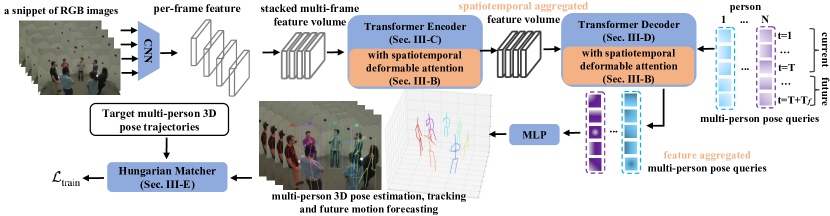
Figure 2: Snipper overview. Taking a snippet of $T$ consecutive RGB images as the input, CNN is used to extract per-frame image features, which are stacked into a multi-frame feature volume. This feature volume is fed into the transformer encoder (Sec. III-D) that employs a novel spatiotemporal deformable attention (Sec. III-C) to aggregate features. Given the spatiotemporally aggregated feature volume from the encoder, the transformer decoder (Sec. III-E) aggregates pose features from it via spatiotemporal deformable attention. Those aggregated pose features are used to update pose queries for $N$ people of $T$ observed frames and $T_{f}$ future frames. The updated queries are regressed to estimate each person’s 3D pose tracking over $T+T_{f}$ frames. We use Hungarian match to find an optimal permutation of a fix set of predicted 3D pose trajectories to a set of target trajectories to compute the multi-person pose losses for training. (Sec. III-F).

Transformer is originally proposed in [54] where self-attention is used and achieves the state-of-art results on many sequence-based tasks. DETR [22] and VisTR [23] are recent inspiring attempts to apply transformer in the end-to-end object detection and instance segmentation. Besides, multi-object tracking with Transformer has also been investigated in [55, 56]. However, due to the high compute requirement of the dot-product attention, both DETR and VisTR can only process low-resolution feature map which limits their accuracy. Deformable attention mechanism is proposed in [24] to tackle this issue, showing strong accuracy for small objects detection. Transformer is recently applied to single person pose estimation, where self-attention module is directly applied to the joint or mesh vertex positions [57, 58, 59], and also multi-frame image features [60, 39]. The most recent work [42] has also employed transformer for multi-person pose estimation, where the query-based self-attention transformer is used to regress multi-person poses for a single frame. To the best of our knowledge, our method is the first to use the deformable attention mechanism for simultaneous multi-person pose estimation, tracking, and forecasting with a single-stage paradigm.

III Method

Snipper is a unified framework that simultaneously addresses three tasks from an RGB video snippet of $T$ observed frames: multi-person 3D pose estimation, tracking, and forecasting for the future $T_{f}$ frames. It consists of four components: image features extractor, transformer encoder (Sec. III-D), decoder (Sec. III-E) and pose trajectory matching for training (Sec. III-F). A novel spatiotemporal deformable attention (III-C) is employed in both the transformer encoder and decoder to aggregate informative pose features shared by the three tasks. To achieve tracking in the entire video, we associate multi-person pose trajectories based on the common frame of two consecutive overlapping snippets with more details presented in the supplementary material. An overview of our pipeline is shown in Fig. 2.

III-A Preliminary

Star pose representation. We represent the 3D human pose as $\mathbf{P}=\{\mathbf{J},\mathbf{V},o\}$ where $\mathbf{J}=\{J_{i}:J_{i}\in\mathrm{R}^{3}\}_{i=1}^{N_{J}}$ is the set of joint locations, $\mathbf{V}=\{V_{i}:V_{i}\in[0,1]\}_{i=1}^{N_{J}}$ is the joint visibility, and $o\in[0,1]$ is the person occurrence probability. Each individual joint position ${J_{i}}$ is modeled by the offset ${J}_{i}^{\text{offset}}=\{\Delta x,\Delta y,\Delta d\}$ from the global root $J^{\text{root}}=\{x,y,d\}$, i.e., $\ J_{i}={J}^{\text{root}}+{J}_{i}^{\text{offset}}$, where $(x,y)$ are the 2D image location of the joint and $d$ is its depth to the camera center, respectively.

Depth and joint offset normalization. As the absolute root depth $d$ depends on the camera focal length $f_{c}$, we normalize the root depth by $\tilde{d}=d/f_{c}$, similar to [35]. In addition, the magnitude of 2D joint offset $(\Delta x,\Delta y)$ is in pixel distance and thus depends on the depth of the person. That is, a person’s joint offset will become smaller if it moves far away from the camera, which tends to make the training in-stable. We mitigate this issue by normalizing the joint offset with the inverse of the normalized root depth, i.e., $\Delta\tilde{x}=\Delta x\cdot\tilde{d}$ and $\Delta\tilde{y}=\Delta y\cdot\tilde{d}$. More details are described in the supplementary material. Thus, the magnitude of 2D normalized joint offset only depends on the pose of the person, which is more consistent across identities. During inference, we assume camera intrinsic is known with a fixed aspect ratio. Otherwise, we use a default focal length and pad the image to the predefined aspect ratio. Finally, a 3D joint position can be converted from the 2.5D joint representation.

III-B Frame-Level Feature Extraction

Given an RGB video snippet of $T$ frames, CNN is used to extract per-frame features of size $H\times W\times C$. We stack these $T$ frame-level features through time and obtain the multi-frame feature volume $\mathbf{F}\in\mathbb{R}^{T\times H\times W\times C}$. Note that the multi-scale pyramid features $\{\mathbf{F}^{l}\}$ extracted by CNN can be easily applied in the followed Transformer Encoder and Decoder for fine-grained spatiotemporal feature extraction. Details are illustrated in Sec. III-C and Fig. 5.

III-C Spatiotemporal Deformable Attention

Spatiotemporal deformable attention module is shown to produce more informative feature for pose tracking from the stack of multi-frame feature volume $\mathbf{F}\in\mathbb{R}^{T\times H\times W\times C}$. (validated in Sec. IV-D) Such aggregation is crucial to mitigate the common inter-frame information missing such as self and partial occlusion.

We summarize our proposed spatiotemporal deformable attention in Fig. 3. Let $q\in\mathbb{R}^{C}$ be the query specified at position $p=(x_{q},y_{q},t_{q})$, where $x_{q},\ y_{q}\in[0,1]$ is the normalized pixel spatial position and $t_{q}$ is the integer frame index of the query $q$. Then, $q$ is passed through two MLPs to regress 2D offsets $\Delta p_{t,k}(q)$ and corresponding attention weights $\alpha_{t,k}(q)$ normalized by the soft-max function. $t$ is an integer specifying the temporal frame in a pre-defined set of neighboring frames $\scriptsize\mathbf{S}(t_{q})=\{t_{q}-1,t_{q},t_{q}+1\}$, and $k$ indexes the offsets on each temporal frame. Note that we do not regress time offset but only 2D spatial offsets $\Delta p_{t,k}$ on each frame of $\mathbf{S}(t_{q})$. We execute this process in parallel by multiple independent heads $h$ and form the final aggregated feature $q_{\text{final}}$ by passing the concatenated feature from each head through a linear layer,

$$q_{\text{final}} =\sum_{h}W^{\prime}_{h}\Big{[}\sum\limits_{t,k}\alpha_{t,k}(q)\cdot W_{h}\mathbf{F}\big{(}p+\Delta p_{t,k}(q)\big{)}\Big{]},$$ (1)

where $W_{h}$ and $W^{\prime}_{h}$ are the parameters of linear layers.

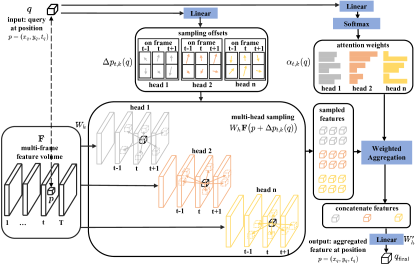
Figure 3: Spatiotemporal deformable attention. Given a volume of stacked multi-frame features, a learnable query $q$, specified at the position $(x_{q},y_{q},t_{q})$, regresses multiple 2D offsets $\Delta p_{t,k}$ to sample features on a set of its neighboring frames $\mathbf{S}(t_{q})$ and the attention weights $\alpha_{t,k}$ to aggregate features. The feature volume is mapped to multiple attention heads with distinct linear layers in parallel, and the accumulated features are concatenated to form the final spatiotemporally aggregated features.

Discussion. There are several alternatives to implement spatiotemporal attention with details displayed in Fig. 4:

• (a) Self-attention. Follow VisTR [23], we flatten multi-frame features to a 2D matrix of shape $THW\times C$ and applies attention to all $THW$ voxels. This attention mechanism is costly for high-resolution feature maps and also breaks the local spatiotemporal relationship for better image-aligned tasks.

• (b) Naïve spatial deformable attention [24]. We reshape the feature volume $\mathbf{F}$ to the shape $H\times W\times CT$, where the channel size becomes $CT$ after concatenating multi-frame temporal features at the same image position. Then the spatial deformable attention is applied on the spatial domain $H\times W$ to aggregate spatiotemporal features. However, this naïve extension fails to consider object or camera motions within a video snippet. With these motions, image features at the same spatial position across frames often change, but the temporal features are still aggregated on the fixed spatial positions.

• (c) Direct 3D sampling: This approach regresses space-time offsets and directly samples in the 3D space $T\times H\times W$, where the interpolation is performed in both spatial and temporal domain, i.e., , $t\in[1,T]$ is fractional instead of integer frame index. However, the temporal interpolation is costly and ill-defined without known correspondences between frames such as optical flow, which leads to defects in the aggregated temporal features.

• (d) Entire snippet sampling: Another scheme is to sample on all frames of the input snippet for the query at $(x_{q},y_{q},t_{q})$, with offsets restricted on each temporal frame in the snippet.

• (e) Neighboring frame sampling (ours): Our approach limits the sampling range to be the immediate neighboring frames $\mathbf{S}(t_{q})$. Despite the short temporal connection at each spatiotemporal deformable attention module, the temporal information is still fully accumulated due to the multiple layers of the attention module in the transformer encoder. Compared with the approaches mentioned above, our proposed mechanism requires less computation, but without any performance reduction. More results and analysis are presented in Sec. IV-D and Fig. 9 that validates the effectiveness and efficiency of our proposed strategy.

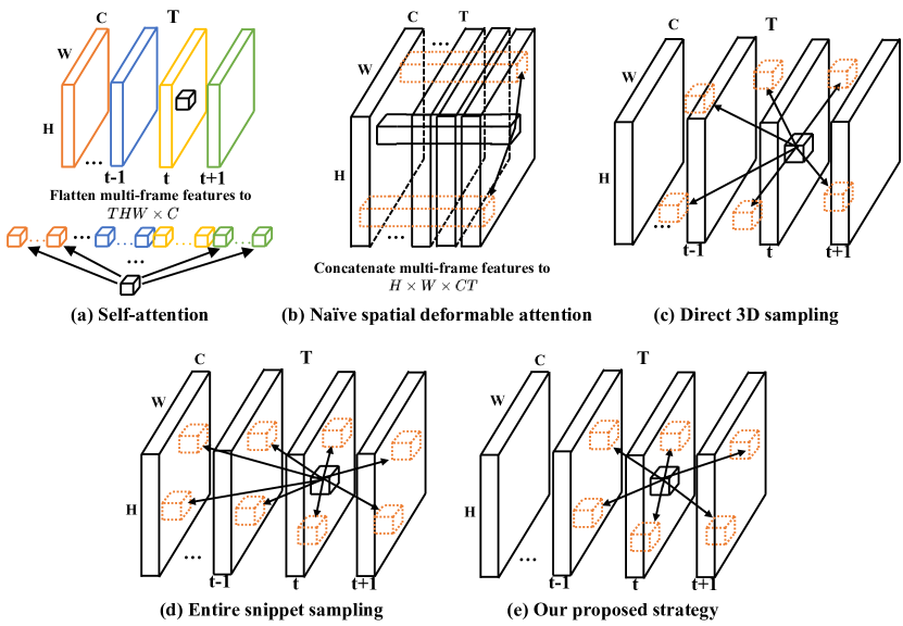
Figure 4: Discussion of different attention mechanisms. (a) Self-attention flattens multi-frame features to $\scriptsize THW\times C$ with attention applied on all $\scriptsize THW$ voxels. (b) Naïve spatial deformable attention concatenates temporal features to $\scriptsize CT\times H\times W$ with deformable attention applied on spatial space $\scriptsize H\times W$. (c) Direct 3D sampling regresses space-time offsets and directly samples in 3D space $\scriptsize T\times H\times W$, where the interpolation is performed in both spatial and temporal domain. (d) Entire snippet sampling performs attention over all the frames within the input snippet. (e) Our proposed spatiotemporal deformable attention samples on neighboring frames efficiently without performance reduction.

Extension to multi-scale features. Our proposed spatiotemporal deformable attention mechanism can be naturally applied to multi-scale multi-frame features extracted by CNN backbone. The process is summarized in Fig. 5. For the query vector $q$ at the position $p=(x_{q},y_{q},t_{q})$, we pass it through two linear layers to regress the sampling offsets $\Delta p_{t,k,l}$ and the attention weights $\alpha_{t,k,l}$ for all scales in parallel, where $l$ indexes the feature volume scale. We use the offsets $\Delta p_{t,k,l}$ to sample the image features at multiple scales and linearly combine these sampled features using the weights $\alpha_{t,k,l}$. This process is mathematically expressed as

$$q_{\text{final}} =\sum_{h}W^{\prime}_{h}\Big{[}\sum\limits_{t,k,l}\alpha_{t,k,l}(q)\cdot W_{h}\mathbf{F}^{l}\big{(}p+\Delta p_{t,k,l}(q)\big{)}\Big{]},$$ (2)

where $W_{h}$ and $W^{\prime}_{h}$ are the parameters of linear layers.

The sampling at the higher scale focuses more on local features with relatively shorter field of perception, while at the lower scale the sampling obtains more global features with relatively broader field of perception. Unlike the self-attention where it is costly to attend to the feature volume globally and unable to extend to multi-scale features, our spatiotemporal deformable attention is efficient as it sparsely sample the image feature and approximates global attention by repeating the sparse sampling for several stages.

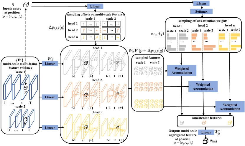
Figure 5: Multi-scale Spatiotemporal Deformable Attention. Given multi-scale (two scales as an example) multi-frame feature volumes, a query vector $q$, specified at position $(x_{q},y_{q},t_{q})$, regresses multiple 2D offsets $\Delta p_{t,k,l}$ to sample features on a set of neighboring frames $\mathbf{S}^{l}(t_{q})$ in all scales of feature volume, as well as corresponding attention weights $\alpha_{t,k,l}$. The sampled features are aggregated and concatenated together to obtain the multi-scale aggregated feature as the output.

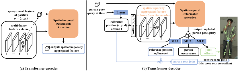
Figure 6: Architecture of transformer encoder and decoder with spatiotemporal deformable attention. (a) In the encoder, for the voxel at position $(x,y,t)$ of multi-frame feature volume $\mathbf{F}$, its voxel feature acts as the query in the attention module to aggregate spatiotemporal features from the feature volume. This process covers every voxel in the volume to create a spatiotemporally aggregated feature volume. (b) In the decoder, a learnable person pose query $q_{t}\in\mathbb{R}^{C}$ at time $t$ first regresses a reference position $(x,y,d)$, and then conducts spatiotemporal deformable attention at the position $(x,y,t)$ of the spatiotemporally aggregated feature volume to aggregate useful pose features. The updated person pose query passes through three MLPs to predict the refinement over reference position $(\Delta x,\Delta y,\Delta d)$, joint offsets $\mathbf{J}^{\text{offsets}}$ with joint visibility $\mathbf{V}$, and the person occurrence probability $o$ at time $t$. The refined reference position is regarded as person root joint and together with joint offsets and occurrence probability, the person’s 3D pose $\mathbf{P}_{t}$ at time $t$ can be constructed.

III-D Spatiotemporal Transformer Encoder

The goal of the transformer encoder is to generate spatiotemporally aggregated feature volume from the CNN-extracted multi-frame features. Fig. 6 (a) describes our transformer encoder with single layer of attention. The encoder consists of multiple layers of attention module where the refined feature volume is used as the input to the next layer and iteratively aggregate spatiotemporal features. Details on multi-layer attention design are given in the supplementary.

Spatiotemporal positional encoding. The position encoding of the pixel location is essential to the transformer attention mechanism. Our encoding scheme follows Wang et al. [23] for a video snippet. Each location $(x,y,t)$ is independently applied to $C/3$ sine and cosine functions with different frequencies as in Vaswani et al. [54] to generate encodings. These encodings are concatenated to form the final $C$ channel positional encoding, which are added to the feature volume $\mathbf{F}$ and fed to the transformer encoder.

Joint heatmap supervision. It is commonly observed that pose estimation is better aligned with the input image if it is regressed from the joint heatmap or body part segmentation [61]. Inspired by Habibie et al. [62], we enforce the first $N_{J}$ channels of each temporal slice in the volume to be the multi-person joints heatmap, denoted by $\mathbf{H}_{t}$. We find empirically that this intermediate supervision improves the 3D pose accuracy (2.9% of 3D-PCK).

III-E Spatiotemporal Transformer Decoder

A person pose query $q\in\mathbb{R}^{C}$ in the decoder is a feature vector or embedding corresponding to a single person’s pose at a specific time. Given a fixed number of $N(T+T_{f})$ learnable person pose queries, the decoder updates these queries by accumulating pose features from the spatiotemporally aggregated feature volume $\mathbf{F}$. These pose queries are used to regresses $N$ people’s 3D pose trajectories in a single shot. Each person’s trajectory consists of $T$ observed poses and $T_{f}$ future poses.

Temporal positional encoding. Since the pose queries of each person are agnostic about the chronological order and need to predict a pose trajectory, we add ${T+T_{f}}$ learnable temporal positional encoding to each query to make it aware of its order before feeding to the transformer decoder. We empirically observe that this helps estimate more accurate 3D pose trajectory in supplementary.

Pose querying. The process is illustrated in Fig. 6 (b). Given a person pose query $q_{t}$ at time $t$, we first regress a reference position $(x,y,d)$ and then conduct spatiotemporal deformable attention at the position $(x,y,t)$ of $\mathbf{F}$. After updating person pose query, it is passed through 3 parallel MLPs to estimate the refinement over the reference position, person occurrence probability at time $t$, and joint offsets with joint visibility. The refined reference position is regarded as the root joint of the person, and we can construct the 3D pose $\mathbf{P}_{t}$ at time $t$ together with the predicted joint offsets and occurrence probability. Similarly, the decoder stacks multiple layers of attention module to iteratively update pose query with detailed design described in the supplementary.

III-F Trajectory Matching Loss

Snipper predicts a fixed number of $N$ people trajectories within the snippet in a single shot, where each trajectory can be represented as $\mathbf{\Gamma}_{i}=\{\mathbf{P}_{t}^{(i)}\}_{t=1}^{T+T_{f}}$. To supervise Snipper, we use Hungarian algorithm [63] to find the optimal matches between the predicted and target pose trajectories, and form the pose trajectory loss for back propagation.

Hungarian matching cost. Let $\mathbf{\Gamma}=\{\mathbf{\Gamma}_{i}\}_{i=1}^{N}$ and $\hat{\mathbf{\Gamma}}=\{\hat{\mathbf{\Gamma}}_{i}\}_{i=1}^{M}$ be the predicted and target pose trajectory sets, respectively. We use Hungarian algorithm to find an optimal permutation $\hat{\sigma}$ of $\mathbf{\Gamma}$ with the lowest bipartite matching cost,

$$\hat{\sigma}=\mathop{\arg\min}_{\sigma}\sum_{i=1}^{M} \mathcal{L}_{\text{occ}}(\mathbf{\Gamma}_{\sigma_{i}},\hat{\mathbf{\Gamma}}_{i})+\mathcal{L}_{\text{traj}}(\mathbf{\Gamma}_{\sigma_{i}},\hat{\mathbf{\Gamma}}_{i})+\mathcal{L}_{\text{vis}}(\mathbf{\Gamma}_{\sigma_{i}},\hat{\mathbf{\Gamma}}_{i}),$$ (3)

where $\mathcal{L}_{\text{occ}}(\mathbf{\Gamma}_{\sigma_{i}},\hat{\mathbf{\Gamma}}_{i})$ is the negative average probability of occurrence,

$$\small\mathcal{L}_{\text{occ}}(\mathbf{\Gamma}_{\sigma_{i}},\hat{\mathbf{\Gamma}}_{i})=-\frac{\sum_{t}\mathds{1}(\hat{o}^{(i)}_{t}\neq\emptyset)\cdot o^{(\sigma_{i})}_{t}}{\sum_{t}\mathds{1}(\hat{o}^{(i)}_{t}\neq\emptyset)},$$ (4)

where $\hat{o}^{(i)}_{t}\neq\emptyset$ means the $i$-th target person occurs at time $t$, $\mathcal{L}_{\text{traj}}(\mathbf{\Gamma}_{\sigma_{i}},\hat{\mathbf{\Gamma}}_{i})$ measures the average $L1$ distance between the predicted and visible target pose trajectory,

$$\small\mathcal{L}_{\text{traj}}(\mathbf{\Gamma}_{\sigma_{i}},\hat{\mathbf{\Gamma}}_{i})=\frac{\sum_{k}\sum_{t}\|\hat{V}^{(i)}_{k,t}\cdot(J^{(\sigma_{i})}_{k,t}-\hat{J}^{(i)}_{k,t})\|_{1}}{\sum_{k}\sum_{t}\hat{V}^{(i)}_{k,t}},$$ (5)

and $\mathcal{L}_{\text{vis}}(\mathbf{\Gamma}_{\sigma_{i}},\hat{\mathbf{\Gamma}}_{i})$ is the average $L2$ distance between the predicted and target joint visibility,

$$\small\mathcal{L}_{\text{vis}}(\mathbf{\Gamma}_{\sigma_{i}},\hat{\mathbf{\Gamma}}_{i})=\frac{\sum_{k}\sum_{t}\|V^{(\sigma_{i})}_{k,t}-\hat{V}^{(i)}_{k,t}\|_{2}^{2}}{N_{j}(T+T_{f})}.$$ (6)

In the above cost definition, we simplify the notations with $\sum_{t}$ as the iteration over all the time steps $\{1,\dots,T+T_{f}\}$, and $\sum_{k}$ as the iteration over all the joints $\{1,\dots,N_{J}\}$ respectively. We follow Carion et al. [22] and adopt the detection probability instead of the log-probabilities in $\mathcal{L}_{\text{occ}}(\mathbf{\Gamma}_{\sigma_{i}},\hat{\mathbf{\Gamma}}_{i})$. We observe better matching behavior between the predicted and target pose trajectories especially for earlier epochs with this strategy.

Training loss. Given the optimal permutation $\hat{\sigma}$, the matched predictions are used to compute both person occurrence and 3D pose losses, and the remaining predictions are only used to compute person occurrence loss. We define the total training loss as

$$\mathcal{L}_{\text{train}}= \sum_{i=1}^{M}\Big{(}\mathcal{L}_{\text{occ}}^{\prime}(\mathbf{\Gamma}_{\hat{\sigma}_{i}},\hat{\mathbf{\Gamma}}_{i})+\mathcal{L}_{\text{traj}}(\mathbf{\Gamma}_{\hat{\sigma}_{i}},\hat{\mathbf{\Gamma}}_{i})+\mathcal{L}_{\text{vis}}(\mathbf{\Gamma}_{\hat{\sigma}_{i}},\hat{\mathbf{\Gamma}}_{i})$$ (7)

$$+\mathcal{L}_{\text{offset}}(\mathbf{\Gamma}_{\hat{\sigma}_{i}},\hat{\mathbf{\Gamma}}_{i})+\mathcal{L}_{\text{smooth}}(\mathbf{\Gamma}_{\hat{\sigma}_{i}},\hat{\mathbf{\Gamma}}_{i})\Big{)}+\mathcal{L}_{\text{heatmap}}(\mathbf{H},\mathbf{\hat{H}}),$$

where $\mathcal{L}^{\prime}_{\text{occ}}$ is the negative log-likelihood for person occurrence prediction,

$$\small\mathcal{L}_{\text{occ}}^{\prime}(\mathbf{\Gamma}_{\hat{\sigma}_{i}},\hat{\mathbf{\Gamma}}_{i})=-\sum_{t}\mathds{1}(\hat{o}^{(i)}_{t}\neq\emptyset)\cdot\log o^{(\hat{\sigma}_{i})}_{t}.$$ (8)

$\mathcal{L}_{\text{traj}}(\mathbf{\Gamma}_{\hat{\sigma}_{i}},\hat{\mathbf{\Gamma}}_{i})$ and $\mathcal{L}_{\text{vis}}(\mathbf{\Gamma}_{\hat{\sigma}_{i}},\hat{\mathbf{\Gamma}}_{i})$ are defined in Eq. 5 and 6 with the permutation replaced with the optimal one $\hat{\sigma}_{i}$ for the computation of training loss.

For the following losses, we drop the superscript $\hat{\sigma}_{i}$ and $i$ for $J^{\text{offset}}$ and $\hat{J}^{\text{offset}}$ for simplicity. $\mathcal{L}_{\text{offset}}(\mathbf{\Gamma}_{\hat{\sigma}_{i}},\hat{\mathbf{\Gamma}}_{i})$ measures the average $L1$ distance between the predicted and target visible joint offsets for the supervision of a single person’s pose,

$$\small\mathcal{L}_{\text{offset}}(\mathbf{\Gamma}_{\hat{\sigma}_{i}},\hat{\mathbf{\Gamma}}_{i})=\frac{\sum_{k}\sum_{t}\|\hat{V}_{k,t}\cdot(J_{k,t}^{\text{offset}}-\hat{J}_{k,t}^{\text{offset}})\|_{1}}{\sum_{k}\sum_{t}\hat{V}_{k,t}},$$ (9)

$\mathcal{L}_{\text{smooth}}(\mathbf{\Gamma}_{\hat{\sigma}_{i}},\hat{\mathbf{\Gamma}}_{i})$ is the average $L2$ smoothness of joint offsets between frames within a video snippet,

$$\small\mathcal{L}_{\text{smooth}}(\mathbf{\Gamma}_{\hat{\sigma}_{i}},\hat{\mathbf{\Gamma}}_{i})=\frac{\sum_{k}\sum_{t}\|J_{k,t}^{\text{offset}}-J_{k,t-1}^{\text{offset}}\|_{2}^{2}}{N_{j}(T+T_{f}-1)},$$ (10)

and $\mathcal{L}_{\text{heatmap}}$ is the average $L2$ distance of joints heatmaps,

$$\small\mathcal{L}_{\text{heatmap}}=\frac{1}{T}\sum_{t}\|\mathbf{H}_{t}-\mathbf{\hat{H}}_{t}\|_{2}^{2}.$$ (11)

Note that while Eq. 5 already captures Eq. 9 to some extents, Eq. 5 couples the root and the offsets, and thus hurts learning. We empirically observe that adding Eq. 9 leads to faster convergence. As the camera motion at each frame is unknown and our predicted root joint is relative to the camera coordinate, $\mathcal{L}_{\text{smooth}}$ factors out the root motion and ensures smooth joints motion.

We apply intermediate pose supervision by computing the losses in Eq. 7, except for the heatmap loss, for each layer of the decoder to guide the learning. Besides, we normalize these losses by the number of target trajectories within a batch such that its magnitude is approximately the same across batches.

IV Experiments

We evaluate on three datasets: JTA [17], CMU-Panoptic [25] and Posetrack2018 [26].

Evaluation Metrics. Our method involves three tasks, multi-person pose estimation, tracking and motion forecasting. For 3D pose estimation, MPJPE is used to evaluate 3D pose accuracy in mm, and MPJPE${}^{\text{rel}}$ means MPJPE after root joint alignment between predicted and target pose. To compare with [11], we report 3D-PCK, where a joint is considered as correct if the distance from the corresponding ground truth joint is less than $150$mm. To compare with [33, 28] on JTA dataset, we also report F1 $@thr\in\{0.4,0.8,1.2\}$ meters, where a joint is considered as correct if the joint position error is less than $thr$. To compare with [10, 17, 48, 64, 47, 50], we report the AP defined in [26] on JTA and Posetrack datasets. For tracking, we follow [26, 14] to report MOTA metrics defined either on 3D or 2D pose. For motion forecasting, we report MPJPE${}^{\text{rel}}$ for 3D pose estimation and 3D path error of root joint, following [18], in Tab. II.

Implementation. We use ResNet50 as the backbone to extract multi-scale features from each image and stack them into a feature volume $\mathbf{F}^{l}$ in chronological order, where $l=\{3,4,5\}$ indexes the convolution stage of feature map. The multi-scale feature volumes are transformed by a $1\times 1$ convolution to be $C=384$ channels. In Snipper, 6 transformer encoder and decoder layers are used with 8 heads in each deformable attention module at the center frame and are halved every frame away from that frame. The head is initialized to have identical attention weights with initial offsets uniformly distributed in angle directions from starting 0 degree. We train Snipper on 8 $V100$ GPUs with batch size of 16 on JTA [17] at 6FPS, CMU-Panoptic [25] at 3FPS Posetrack2018 [26] at 7.5 FPS, and COCO, where we apply 2D transformation to make it become a video snippet, jointly. We use 14 joints format in MPII [65] common across all datasets.

TABLE I: Quantitative evaluations of 3D pose tracking on JTA dataset. We compare with three bottom-up (BU) methods [10, 17, 28], a single-stage (SS) method [11], and a hybrid of bottom-up and top-down (TD) method [33]. Ours (${\scriptstyle T=1}$) and Ours (${\scriptstyle T=4}$) are the evaluations of model trained on a snippet of 1 and 4 frames. Ours (${\scriptstyle t=4+1}$) and Ours (${\scriptstyle t=4+2}$) are the evaluations of motion forecasting for the 1st and 2nd future frame based on the observed snippet of 4 frames. Snipper outperforms prior works on both tasks. Underline means the second best results.

Method		Pose Estimation					Tracking
		AP	F1$@0.4$m	F1$@0.8$m	F1$@1.2$m	3D-PCK	MOTA
OpenPose(2019) [10]	BU	50.1	-	-	-	-	-
THOPA(2019) [17]	BU	59.3	-	-	-	-	59.3
LoCOn(2020) [28]	BU	-	50.8	64.8	70.4	-	-
PandaNet(2020) [11]	SS	-	-	-	-	83.2	-
Cheng et al.(2021) [33]	BU+TD	-	57.2	68.5	72.9	-	-
Ours (${\scriptstyle t=4+1}$)	SS	66.5	56.2	67.9	73.1	83.8	-
Ours (${\scriptstyle t=4+2}$)	SS	64.5	53.2	65.9	71.2	82.8	-
Ours (${\scriptstyle T=1}$)	SS	65.3	59.7	70.7	75.7	83.4	61.4
Ours (${\scriptstyle T=4}$)	SS	70.5	60.3	71.5	76.4	85.7	63.2

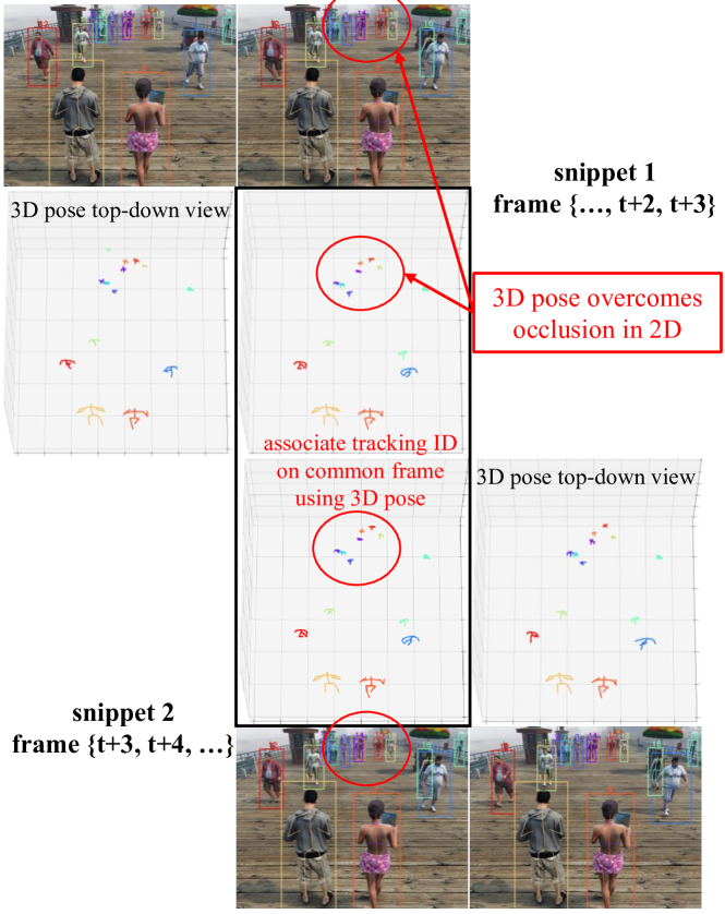
Figure 8: Association between Two Consecutive Snippets. To achieve multi-person tracking over the whole video, for two consecutive snippets (${\scriptstyle T=4}$) consisting of frames $\scriptstyle\{t,...,t+3\}$ and $\scriptstyle\{t+3,...,t+6\}$, the association of 3D pose tracking is based on the common frame $\scriptstyle t+3$. The 3D pose association helps overcome the occlusion on 2D images.

Ours (${\scriptstyle T=1}$) and Ours (${\scriptstyle T=4}$) denote the evaluation of model trained on a snippet of 1 and 4 frames. For fair comparison in each dataset, we train and test our model on the corresponding dataset only following prior work. To achieve multi-person tracking over the whole video, for two consecutive snippets (${\scriptstyle T=4}$) consisting of frames $\{t,...,t+3\}$ and $\{t+3,...,t+6\}$, the association of 3D pose tracking is based on the common frame $t+3$ with the nearest 3D pose matching measured in Euclidean distance. The process is shown in Fig. 8. For snippet (${\scriptstyle T=1}$), whole-video tracking is achieved by Hungarian matching on poses of two consecutive frames. For motion forecasting, ${\scriptstyle T_{f}=2}$ is used based on ${\scriptstyle T=4}$ observed frames. Ours (${\scriptstyle t=4+1}$) and Ours (${\scriptstyle t=4+2}$) denote the evaluation on predicted pose of the 1st and 2nd future frame. The inference time is 76ms and 266ms in average for a single snippet of 1 and 4 frames on JTA dataset on a single $V100$ GPU, and the number of parameters is 40M and 43M respectively.

IV-A JTA Evaluation

For JTA dataset, we resize the input image to the resolution $540\times 960$ and downsample the video to 6 FPS. Since there is no prior work evaluating all the three tasks on JTA dataset, we present the results from our method in Tab. I and compare with the state-of-art methods on multi-person 3D pose estimation, tracking and motion forecasting. For pose estimation, comparing with the single-stage PanadaNet [11], our method estimates 0.2% and 2.5% better 3D-PCK for Ours (${\scriptstyle T=1}$) and Ours (${\scriptstyle T=4}$), respectively. Compared with [28, 33], Ours (${\scriptstyle T=4}$) shows around 10% and 3% of F1$@0.4$m increase. For tracking, Ours (${\scriptstyle T=4}$) is around 4% more accurate in MOTA than THOPA [17]. For motion forecasting, Ours (${\scriptstyle T=4}$) can predict competitive future motion that outperforms methods that do prediction on the hidden future images  [10, 17, 30], even with a single-stage architecture (e.g. , 66.5, 64.5 of F1@0.4m and 83.8, 82.8 of 3D-PCK for the 2 future frames). In Tab. II, we compare our method with HMP [18], the only work to forecast 3D pose from RGB images, on motion forecasting of next 2 frames. Our method estimates comparable pose forecasting as HMP but outperforms it when noise is added to the history pose in HMP, highlighting the benefit of solving the pose estimation, tracking and forecasting in a joint framework. These accuracy improvement is rooted in the effectiveness of the spatiotemporal deformable attention.

The evaluation of motion forecasting on JTA dataset is presented in Tab. II. No forecasting means to keep the last observed pose for evaluation without motion prediction. For fair comparison, we retrain HMP [18] to take only 4 frames as input and forecast the next 2 frames. The evaluation is done for the deterministic mode of HMP. We use the ground truth history 2D pose in $\text{HMP}^{1}$ but added Gaussian noise $\mathcal{N}(0,3)$ pixels to the ground truth history 2D pose for $\text{HMP}^{2}$. HMP (Hourglass), means HMP is trained with 2D poses estimated by Hourglass [43]. Our method jointly estimates the poses in the observed frames and forecasts its motion, which shows comparable accuracy with noise-free HMP but noticeably outperforms it when adding noise to the history pose or using the estimated poses.

TABLE II: Quantitative evaluations of motion forecasting on JTA dataset. Our method shows comparable accuracy with noise-free HMP but noticeably outperforms it when adding noise to the history pose or using the estimated poses

Method	3D Path Error (mm)		MPJPE${}^{\text{rel}}$ (mm)
Forecasting Time	166ms	333ms	166ms	333ms
No forecasting	353.5	409.1	123.5	139.1
$\text{HMP}^{1}$ [18]	90.3	112.6	35.4	39.5
$\text{HMP}^{2}$ [18]	94.5	121.8	48.5	61.4
HMP (Hourglass [43])	95.2	123.3	46.8	60.6
Ours	92.3	117.7	37.9	43.0

IV-B CMU-Panoptic Evaluation

For multi-person pose estimation or tracking, there are mainly 2 protocols of data split used in prior works [11, 14]. Protocol 1 follows [14] where 3 views HD cameras ($3,13,23$) and all the haggling videos of version 1.2 are used. The training and testing video split follows [14, 66], and the evaluation metrics follow [14, 12]. Protocol 2 follows [11, 28] where 4 scenarios (Haggling, Mafia, Ultimatum, Pizza) are selected. The testing set is composed of HD videos of camera 16 and 30, and the training set includes videos of other 28 cameras. The evaluation metrics follow [11, 28]. Since the speed motion of this dataset is slower than JTA dataset, we downsample to 3 FPS to avoid too much redundancy during training and use the image resolution $540\times 960$ as the input. We also provide test results of 6 FPS with the model trained on 3 FPS, denoted by Ours (${\scriptstyle T=4}$, 6 FPS).

TABLE III: Quantitative evaluations on CMU-Panoptic of protocol 1. Our method shows competitive or higher accuracy than three top-down approaches [12, 14, 53], and gives competitive accuracy of motion forecasting. Underline means the second best results.

Method		Backbone	MPJPE	MPJPE${}^{\text{rel}}$	MOTA
VoxelPose(2020) [12]	TD	ResNet50	66.9	51.1	-
TesseTrack(2021) [14]	TD	HRNet	18.9	-	76.0
VoxelTrack(2022) [53]	TD	DLA-34	66.4	-	-
Ours (${\scriptstyle t=4+1}$)	SS	ResNet50	49.0	40.8	-
Ours (${\scriptstyle t=4+2}$)	SS	ResNet50	50.7	41.3	-
Ours (${\scriptstyle T=4}$, 6 FPS)	SS	ResNet50	45.1	37.3	80.9
Ours (${\scriptstyle T=1}$)	SS	ResNet50	48.4	37.5	78.1
Ours (${\scriptstyle T=4}$)	SS	ResNet50	44.3	37.1	81.7

TABLE IV: Quantitative evaluations on CMU-Panoptic of protocol 2. Our single-stage (SS) method outperforms two bottom-up [29, 28] and three single-stage methods [11, 41, 40, 46] and gives competitive accuracy of motion forecasting.

Method		MPJPE					F1	MOTA
		Hag.	Maf.	Ult.	Piz.	Avg.
MubyNet(2018) [29]	BU	72.4	78.8	66.8	94.3	72.1	-	-
LoCO(2020) [28]	BU	45	95	58	79	69	89.2	-
PandaNet(2020) [11]	SS	40.6	37.6	31.3	55.8	42.7	-	-
Benzine et al.(2021) [46]	SS	70.1	66.6	55.6	78.4	68.5	-	-
Jin et al.(2022) [40]	SS	63.7	58.5	52.3	69.1	60.9	-	-
Wang et al.(2022) [41]	SS	53.3	51.2	49.1	61.5	53.8	-	-
Ours (${\scriptstyle t=4+1}$)	SS	41.4	38.8	41.6	44.9	40.3	88.7	-
Ours (${\scriptstyle t=4+2}$)	SS	43.0	40.9	42.9	47.4	42.4	85.5	-
Ours (${\scriptstyle T=4}$, 6 FPS)	SS	37.3	37.1	39.0	42.6	38.2	90.0	93.0
Ours (${\scriptstyle T=1}$)	SS	37.6	38.5	39.7	45.0	39.4	89.4	92.9
Ours (${\scriptstyle T=4}$)	SS	36.8	36.9	38.6	42.5	37.9	90.1	93.4

The results of protocol 1 are shown in Tab. III. Our method outperforms VoxelPose [12]: 22.6mm (+33%) on MPJPE and 14mm (+27%) on relative MPJPE. As for its following work VoxelTrack [53], we also exceeds 22.1mm on MPJPE. Compare with TesseTrack [14], Ours (${\scriptstyle T=4}$) shows higher pose tracking accuracy (81.7 vs 76.0 of MOTA), but lower accuracy on MPJPE, which might be because TesseTrack uses HRNet as the backbone (around 100M parameters) while ours only uses ResNet50 (43M parameters). For protocol 2, we show comparison with six recent works [29, 28, 11, 46, 40, 41] in Tab. IV. Snipper performs better on F1 scores and MPJPE in all six sequences except for the Ultimatum sequence, where PandaNet [11] achieves 7.3mm lower than ours. For tracking, Snipper achieves over 90% MOTA. For motion prediction, ours (${\scriptstyle t=T+1}$) and ours (${\scriptstyle t=T+2}$) in both protocol 1 and 2 have competitive results on MPJPE, only about 3 and 5mm of worse than ours (${\scriptstyle T=4}$) with the observed motion (see Tab. IV).

IV-C Posetrack2018 Evaluation

TABLE V: Quantitative evaluations (AP) of pose estimation on Posetrack2018 val set.

Method		Head	Sho	Elb	Wri	Hip	Kne	Ank	Avg
DetTrack(2020) [48]	TD	84.9	87.4	84.8	79.2	77.6	79.7	75.3	81.5
PT_CPN++(2018) [64]	TD	82.4	88.8	86.2	79.4	72.0	80.6	76.2	80.9
TML++(2019) [47]	BU	-	-	-	-	-	-	-	74.6
STAF(2019) [50]	BU	-	-	-	64.7	-	-	62.0	70.4
Ours (${\scriptstyle T=1}$)	SS	86.5	85.6	71.5	67.9	78.1	72.0	62.6	74.9
Ours (${\scriptstyle T=4}$)	SS	86.7	85.9	71.6	68.6	78.3	72.5	63.6	75.3

TABLE VI: Quantitative evaluations (MOTA) of tracking on Posetrack2018 val set.

Method		Head	Sho	Elb	Wri	Hip	Kne	Ank	Avg
DetTrack(2020) [48]	TD	74.2	76.4	71.2	64.1	64.5	65.8	61.9	68.7
PT_CPN++(2018) [64]	TD	68.8	73.5	65.6	61.2	54.9	64.6	56.7	64.0
Rajasegaran et al.(2021) [15]	TD	-	-	-	-	-	-	-	55.8
Rajasegaran et al.(2022) [52]	TD	-	-	-	-	-	-	-	58.9
TML++(2019) [47]	BU	76.0	76.9	66.1	56.4	65.1	61.6	52.4	65.7
STAF(2019) [50]	BU	-	-	-	-	-	-	-	60.9
Ours (${\scriptstyle T=1}$)	SS	82.0	82.0	58.8	53.8	72.3	61.1	40.2	64.2
Ours (${\scriptstyle T=4}$)	SS	82.1	82.3	59.0	53.7	72.7	61.7	41.7	64.7

We use Posetrack2018 [26] to validate that our method is flexible to 2D pose tracking task by simply skipping joint depth prediction. Since the provided annotations of PoseTrack2018 dataset is in 7.5 FPS, we downsample the input video to 7.5 FPS accordingly in both training and testing. We report our results on the validation set following prior works [48, 47, 50]. Tab. V and VI present the results of Snipper on 2D pose estimation (AP) and pose tracking (MOTA). When comparing with bottom-up approaches, our method exceeds STAF [50] for about 4% in AP and MOTA, and also shows competitive results with TML++ [47]. For the most recent top-down methods [48], our method is around 6% AP and 4% MOTA worse, which could attribute to the fact that our method jointly performs multi-person detection and pose tracking, while [48] relies on a specialized person detector to obtain the multi-person detection. When comparing with the most recent works [15, 52], our method still achieves around 8.9% and 5.8% MOTA better, which is largely credited to the inclusion of pose estimation that helps robust tracking.

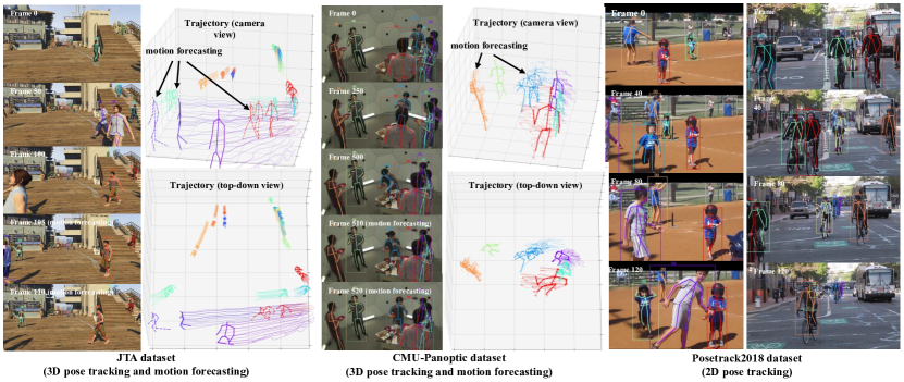
Figure 7: Qualitative results on JTA, CMU Panoptic and Posetrack2018 datasets. We show 3D pose tracking and motion forecasting results on JTA and CMU Panoptic datasets, and 2D pose tracking results on Posetrack dataset. Dashed 3D poses are the forecasting motion based on the last observed snippet.

IV-D Ablation Study

We present several key ablation studies (discussed in Sec. III-C) on JTA dataset to highlight effectiveness and efficiency of our proposed spatiotemporal deformable attention and the correlation between pose estimation and tracking in Tab. VII. The comparison of five attention strategies in terms of training time v.s. performance is shown in Fig. 9 to illustrate the effectiveness and efficiency of our proposed attention module. More ablation studies are provided in the supplementary.

TABLE VII: Quantitative results of ablation study on JTA dataset.

	3D Pose Estimation					Tracking
Method	AP	F1$@0.4$m	F1$@0.8$m	F1$@1.2$m	3D-PCK	MOTA
Self attention	53.2	42.0	55.0	62.4	71.0	49.9
Spatial deform. att.	69.0	53.8	69.3	75.3	84.4	62.3
Direct 3D sampl.	62.8	54.3	65.0	71.6	83.2	55.9
Entire snippet	71.2	59.3	70.3	76.2	85.0	63.4
Ours (single scale)	54.5	43.1	56.8	64.1	73.4	50.2
Ours (2D bbx tracking)	66.5	58.1	69.0	71.8	81.9	54.6
Ours (2D pose tracking)	67.1	59.5	69.3	73.4	83.3	55.9
Ours (w/o smooth loss)	69.1	59.7	70.7	75.9	86.1	62.4
Ours (1 FPS)	68.5	58.8	69.1	73.4	84.0	62.1
Ours (30 FPS)	69.2	59.2	70.5	75.2	84.2	62.7
Ours	70.5	60.3	71.5	76.4	85.7	63.2

Self-attention [23]. Our method outperforms self-attention (more than 20% in all metrics), which is due to two main factors: (1) destruction of spatiotemporal local context within multi-frame features and (2) prohibitive compute for high-resolution multi-scale image features needed to estimate pose of small people.

Naïve spatial deformable attention [24]. This strategy performs slightly worse than ours, especially for accurate pose estimation (53.8 vs 60.3 of F1$@0.4$m) as it neglects scene/camera/object motions through time, where the temporal features at the same image position are not corresponding.

Direct 3D sampling. This strategy also outperforms self-attention, showing that deformable attention in 3D space is an essential technique to encode spatiotemporal information from multi-frame features. However, it is still worse than ours by a large margin, mainly because the interpolation in temporal domain is ill-defined without known correspondences between frames such as optical flow, which leads to the aggregated features incorrect in time.

Entire snippet sampling. Our mechanism requires less computation cost and takes only 50% training time of model with attention over the entire snippet, but gives similar performance, which showcases the efficiency of our approach.

Ours (2D pose tracking) and Ours (bbx tracking) means the association between snippets is based on 2D pose or 2D bounding box instead of 3D pose, which reduces 7.3% on MOTA and 2% on 3D-PCK for 2D pose and 8.6% and 3.4% for 2D bounding box. Compared to 2D pose, 3D pose alleviates the issues of occlusion between people on an image since depth information is considered, which demonstrates that effective pose estimation facilitates tracking.

Ours (w/o smooth loss) denotes the model trained without joint smoothness loss $\mathcal{L}_{\text{smooth}}$ in Eq. 7 for a snippet of 4 frames as the input. The pose scores are lower than our full model, illustrating that contextual information for tracking also helps improve pose estimation. However, this model without the smoothness loss still performs better than our model but with 1-frame input, indicating the effectiveness of the spatiotemporal attention model.

Ours (1 FPS) and Ours (30 FPS) denote the model trained with video snippets at 1 FPS and 30 FPS respectively. The pose tracking performances are slightly worse than using 6 FPS, which can be the factor that very high frame rate introduces too much redundancy and easily results in overfitting during training while very low frame rate introduces too much discrepancy and results in missing clues for tracking and forecasting.

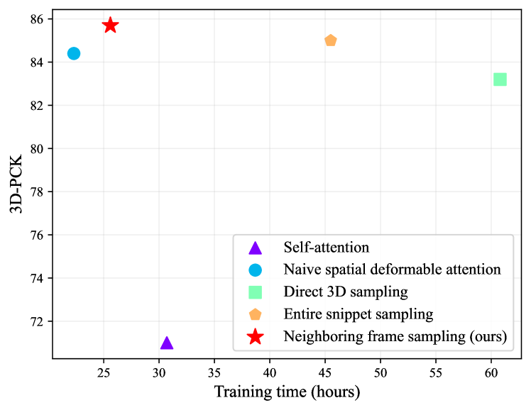
Figure 9: Comparison of five attention strategies in terms of training time v.s. performance (3D-PCK). We show the effectiveness and efficiency of our proposed spatiotemporal attention module. Training setting is identical for all five cases.

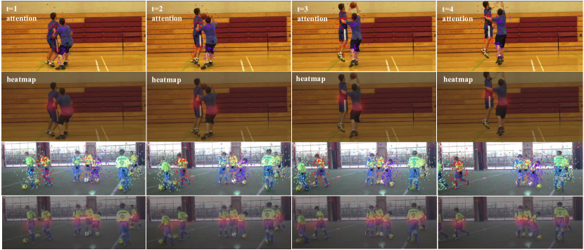
Figure 10: Visualization of deformable attention in the transformer decoder and heatmaps of root joint. (best viewed in color) The sampling positions of the deformable attention for each person’s pose query are displayed in the same color and “$\times$” means the predicted root joint position. We show that the sampling positions of deformable attention usually cover the whole body of each person for effective and efficient pose feature accumulation.

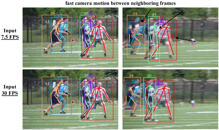
Figure 11: Failure case. Our method using video snippet at 7.5 FPS as input for inference could suffer from fast camera motion due to the large discrepancies between neighboring frames. In this special case, when we use video snippet at 30 FPS for inference, the model gives much better results due to the preserved correlation between frames in the input video, despite of fast camera motions.

IV-E Discussion

Correlations among three tasks. Pose estimation and tracking are correlated with each other. The accurate 3D poses facilitate tracking, whereas robust tracking provides the informative temporal clues for pose estimation within the snippet. This is validated by comparing the consistent better pose estimation and tracking performance of Ours (${\scriptstyle T=4}$) than Ours (${\scriptstyle T=1}$) or multi-stage methods [28, 12, 34, 52] on the three datasets in Tab. I, III, IV, V and VI.

On the other hand, pose tracking builds the crucial history for motion forecasting demonstrated by the better forecast motion of Ours than no forecasting in Tab. II. Though in this paper, we cannot demonstrate that motion forecasting in turn helps pose tracking, We include the important task of motion forecasting in our unified framework for another two purposes: efficiency and robustness. For efficiency, the encoded spatiotemporal features within the video snippet capture crucial history for motion forecasting. Thus we can address the three tasks in a single stage with our unified framework for efficiency, i.e. running one network vs. many networks. TesseTrack [14] ($\sim$100M params) addresses only pose tracking, while our method (only 43M params) addresses all three tasks. For robustness, existing work on motion forecasting uses off-the-shelf pose estimators, such as HMP [18], for the history pose estimation. But the pose estimators could fail unpredictably and thus cause forecasting to fail. Solving them jointly can be robust to pose tracking errors. We validate that our unified framework helps motion forecasting in Tab. II, where our method shows better performance than the multi-stage method HMP (Hourglass [43]).

Generalization ability. To validate the generalization ability of our method, we train our model on a hybrid of datasets, MuCo [67], COCO [68], Posetrack2018 [26] and JTA [17]. Then we test our model to predict 3D pose tracking on the unseen MuPoTS [67] and Posetrack val set (no 3D pose annotations). The qualitative results are included in the supplementary video, where the predicted 3D pose is smooth and the tracking is consistent across the entire videos, even in occlusion cases.

Attention visualization. We visualize the attention maps of the last layer in the transformer decoder in Fig. 10, where the sampling positions for each person’s pose queries are presented by the same color and “$\times$” means the root joint position. Our proposed spatiotemporal deformable attention samples around each person’s whole body and later aggregates these sampled features together to update pose queries. Compared with self-attention, our proposed deformable attention typically preserves better spatial and temporal relationships for correct pose regression, and compared with the naïve spatial deformable attention, our method considers the motion changes between frames as is indicated by the root joint positions ”$\times$” of each person in the video snippet in Fig. 10.

Failure case and limitations. Our method could suffer frame fast camera motion as shown in Fig. 11, where there are quite large discrepancies between neighboring frames at 7.5 FPS. In this special case, the problem can be alleviated when we use video snippet at 30 FPS as the input due to the preserved correlation between frames. Another limitation lies in the spatiotemporal positional encoding that does not consider the correspondence between frames, especially the camera motion exists between frames. Future work could explore explicitly use the camera poses such as ray-based position encoding and the low-resolution optical flow to guide the feature aggregation.

V Conclusion

We present Snipper, a unified spatiotemporal Transformer for simultaneous multi-person 3D pose estimation, tracking and motion forecasting on a video snippet. We propose an efficient yet powerful spatiotemporal deformable attention module to aggregate spatiotemporal information across the snippet. We demonstrate the effectiveness of Snipper on three challenging public datasets where a generic Snipper model rivals specialized state-of-art baselines trained for 3D pose estimation, tracking, and forecasting.

References

- [1] Y.-F. Song, Z. Zhang, C. Shan, and L. Wang, “Richly activated graph convolutional network for robust skeleton-based action recognition,” IEEE Transactions on Circuits and Systems for Video Technology, vol. 31, no. 5, pp. 1915–1925, 2020.
- [2] Z. Sun, J. Chen, L. Chao, W. Ruan, and M. Mukherjee, “A survey of multiple pedestrian tracking based on tracking-by-detection framework,” IEEE Transactions on Circuits and Systems for Video Technology, vol. 31, no. 5, pp. 1819–1833, 2021.
- [3] T. L. Munea, Y. Z. Jembre, H. T. Weldegebriel, L. Chen, C. Huang, and C. Yang, “The progress of human pose estimation: a survey and taxonomy of models applied in 2d human pose estimation,” IEEE Access, 2020.
- [4] C. Benedek, B. Gálai, B. Nagy, and Z. Jankó, “Lidar-based gait analysis and activity recognition in a 4d surveillance system,” IEEE Transactions on Circuits and Systems for Video Technology, vol. 28, no. 1, pp. 101–113, 2016.
- [5] X. Wang, L. Gao, Y. Zhou, J. Song, and M. Wang, “Ktn: Knowledge transfer network for learning multi-person 2d-3d correspondences,” IEEE Transactions on Circuits and Systems for Video Technology, 2022.
- [6] J. Li and M. Wang, “Multi-person pose estimation with accurate heatmap regression and greedy association,” IEEE Transactions on Circuits and Systems for Video Technology, vol. 32, no. 8, pp. 5521–5535, 2022.
- [7] R. Gu, G. Wang, Z. Jiang, and J.-N. Hwang, “Multi-person hierarchical 3d pose estimation in natural videos,” IEEE Transactions on Circuits and Systems for Video Technology, vol. 30, no. 11, pp. 4245–4257, 2019.
- [8] A. Martínez-González, M. Villamizar, O. Canévet, and J.-M. Odobez, “Efficient convolutional neural networks for depth-based multi-person pose estimation,” IEEE Transactions on Circuits and Systems for Video Technology, vol. 30, no. 11, pp. 4207–4221, 2020.
- [9] G. Wei, C. Lan, W. Zeng, and Z. Chen, “View invariant 3d human pose estimation,” IEEE Transactions on Circuits and Systems for Video Technology, vol. 30, no. 12, pp. 4601–4610, 2019.
- [10] Z. Cao, G. Hidalgo, T. Simon, S.-E. Wei, and Y. Sheikh, “OpenPose: realtime multi-person 2d pose estimation using part affinity fields,” IEEE Transactions on Pattern Analysis and Machine Intelligence, vol. 43, no. 1, pp. 172–186, 2019.
- [11] A. Benzine, F. Chabot, B. Luvison, Q. C. Pham, and C. Achard, “PandaNet: Anchor-based single-shot multi-person 3d pose estimation,” in IEEE/CVF Conference on Computer Vision and Pattern Recognition, 2020, pp. 6856–6865.
- [12] H. Tu, C. Wang, and W. Zeng, “VoxelPose: Towards multi-camera 3d human pose estimation in wild environment,” in European Conference on Computer Vision, 2020, pp. 197–212.
- [13] S. Zou, X. Zuo, S. Wang, Y. Qian, C. Guo, and L. Cheng, “Human pose and shape estimation from single polarization images,” IEEE Transactions on Multimedia, 2022.
- [14] N. D. Reddy, L. Guigues, L. Pishchulin, J. Eledath, and S. G. Narasimhan, “TesseTrack: End-to-end learnable multi-person articulated 3d pose tracking,” in IEEE/CVF Conference on Computer Vision and Pattern Recognition, 2021, pp. 15 190–15 200.
- [15] J. Rajasegaran, G. Pavlakos, A. Kanazawa, and J. Malik, “Tracking people with 3d representations,” in Annual Conference on Neural Information Processing Systems, 2021.
- [16] B. Xiao, H. Wu, and Y. Wei, “Simple baselines for human pose estimation and tracking,” in European Conference on Computer Vision, 2018, pp. 466–481.
- [17] M. Fabbri, F. Lanzi, S. Calderara, A. Palazzi, R. Vezzani, and R. Cucchiara, “Learning to detect and track visible and occluded body joints in a virtual world,” in European Conference on Computer Vision, 2018, pp. 430–446.
- [18] Z. Cao, H. Gao, K. Mangalam, Q.-Z. Cai, M. Vo, and J. Malik, “Long-term human motion prediction with scene context,” in European Conference on Computer Vision, 2020.
- [19] R. Villegas, J. Yang, Y. Zou, S. Sohn, X. Lin, and H. Lee, “Learning to generate long-term future via hierarchical prediction,” in IEEE International Conference on Machine Learning. PMLR, 2017, pp. 3560–3569.
- [20] J. Walker, K. Marino, A. Gupta, and M. Hebert, “The pose knows: Video forecasting by generating pose futures,” in IEEE/CVF International Conference on Computer Vision, 2017, pp. 3332–3341.
- [21] A. Gupta, J. Johnson, L. Fei-Fei, S. Savarese, and A. Alahi, “Social gan: Socially acceptable trajectories with generative adversarial networks,” in IEEE/CVF Conference on Computer Vision and Pattern Recognition, 2018, pp. 2255–2264.
- [22] N. Carion, F. Massa, G. Synnaeve, N. Usunier, A. Kirillov, and S. Zagoruyko, “End-to-end object detection with transformers,” in European Conference on Computer Vision, 2020, pp. 213–229.
- [23] Y. Wang, Z. Xu, X. Wang, C. Shen, B. Cheng, H. Shen, and H. Xia, “End-to-end video instance segmentation with transformers,” in IEEE/CVF Conference on Computer Vision and Pattern Recognition, 2021, pp. 8741–8750.
- [24] X. Zhu, W. Su, L. Lu, B. Li, X. Wang, and J. Dai, “Deformable DETR: Deformable transformers for end-to-end object detection,” arXiv preprint arXiv:2010.04159, 2020.
- [25] H. Joo, T. Simon, X. Li, H. Liu, L. Tan, L. Gui, S. Banerjee, T. Godisart, B. Nabbe, I. Matthews et al., “Panoptic studio: A massively multiview system for social interaction capture,” IEEE Transactions on Pattern Analysis and Machine Intelligence, vol. 41, no. 1, pp. 190–204, 2017.
- [26] M. Andriluka, U. Iqbal, E. Insafutdinov, L. Pishchulin, A. Milan, J. Gall, and B. Schiele, “PoseTrack: A benchmark for human pose estimation and tracking,” in IEEE/CVF Conference on Computer Vision and Pattern Recognition, 2018.
- [27] L. Pishchulin, E. Insafutdinov, S. Tang, B. Andres, M. Andriluka, P. V. Gehler, and B. Schiele, “Deepcut: Joint subset partition and labeling for multi person pose estimation,” in IEEE/CVF Conference on Computer Vision and Pattern Recognition, 2016, pp. 4929–4937.
- [28] M. Fabbri, F. Lanzi, S. Calderara, S. Alletto, and R. Cucchiara, “Compressed volumetric heatmaps for multi-person 3d pose estimation,” in IEEE/CVF Conference on Computer Vision and Pattern Recognition, 2020, pp. 7204–7213.
- [29] A. Zanfir, E. Marinoiu, M. Zanfir, A.-I. Popa, and C. Sminchisescu, “Deep network for the integrated 3d sensing of multiple people in natural images,” in Annual Conference on Neural Information Processing Systems, 2018, pp. 8410–8419.
- [30] Y. Chen, Z. Wang, Y. Peng, Z. Zhang, G. Yu, and J. Sun, “Cascaded pyramid network for multi-person pose estimation,” in IEEE/CVF Conference on Computer Vision and Pattern Recognition, 2018, pp. 7103–7112.
- [31] R. Girdhar, G. Gkioxari, L. Torresani, M. Paluri, and D. Tran, “Detect-and-track: Efficient pose estimation in videos,” in IEEE/CVF Conference on Computer Vision and Pattern Recognition, 2018, pp. 350–359.
- [32] G. Moon, J. Y. Chang, and K. M. Lee, “Camera distance-aware top-down approach for 3d multi-person pose estimation from a single rgb image,” in IEEE/CVF International Conference on Computer Vision, 2019, pp. 10 133–10 142.
- [33] Y. Cheng, B. Wang, B. Yang, and R. T. Tan, “Monocular 3d multi-person pose estimation by integrating top-down and bottom-up networks,” in IEEE/CVF Conference on Computer Vision and Pattern Recognition, 2021, pp. 7649–7659.
- [34] C. Wang, J. Li, W. Liu, C. Qian, and C. Lu, “Hmor: Hierarchical multi-person ordinal relations for monocular multi-person 3d pose estimation,” in European Conference on Computer Vision. Springer, 2020, pp. 242–259.
- [35] Y. Cheng, B. Wang, B. Yang, and R. T. Tan, “Graph and temporal convolutional networks for 3d multi-person pose estimation in monocular videos,” in Proceedings of the AAAI Conference on Artificial Intelligence, vol. 35, no. 2, 2021, pp. 1157–1165.
- [36] D. Mehta, O. Sotnychenko, F. Mueller, W. Xu, M. Elgharib, P. Fua, H.-P. Seidel, H. Rhodin, G. Pons-Moll, and C. Theobalt, “Xnect: Real-time multi-person 3d motion capture with a single rgb camera,” ACM Transactions on Graphics, vol. 39, no. 4, pp. 82–1, 2020.
- [37] X. Nie, J. Feng, J. Zhang, and S. Yan, “Single-stage multi-person pose machines,” in IEEE/CVF International Conference on Computer Vision, 2019.
- [38] Y. Sun, Q. Bao, W. Liu, Y. Fu, M. J. Black, and T. Mei, “Monocular, one-stage, regression of multiple 3d people,” in IEEE/CVF Conference on Computer Vision and Pattern Recognition, 2021, pp. 11 179–11 188.
- [39] T. Wang, J. Zhang, Y. Cai, S. Yan, and J. Feng, “Direct multi-view multi-person 3d human pose estimation,” in Annual Conference on Neural Information Processing Systems, 2021.
- [40] L. Jin, C. Xu, X. Wang, Y. Xiao, Y. Guo, X. Nie, and J. Zhao, “Single-stage is enough: Multi-person absolute 3d pose estimation,” in Proceedings of the IEEE/CVF Conference on Computer Vision and Pattern Recognition, 2022, pp. 13 086–13 095.
- [41] Z. Wang, X. Nie, X. Qu, Y. Chen, and S. Liu, “Distribution-aware single-stage models for multi-person 3d pose estimation,” in Proceedings of the IEEE/CVF Conference on Computer Vision and Pattern Recognition, 2022, pp. 13 096–13 105.
- [42] D. Shi, X. Wei, L. Li, Y. Ren, and W. Tan, “End-to-end multi-person pose estimation with transformers,” in Proceedings of the IEEE/CVF Conference on Computer Vision and Pattern Recognition, 2022, pp. 11 069–11 078.
- [43] A. Newell, K. Yang, and J. Deng, “Stacked hourglass networks for human pose estimation,” in European Conference on Computer Vision. Springer, 2016, pp. 483–499.
- [44] G. Rogez, P. Weinzaepfel, and C. Schmid, “Lcr-net++: Multi-person 2d and 3d pose detection in natural images,” IEEE Transactions on Pattern Analysis and Machine Intelligence, vol. 42, no. 5, pp. 1146–1161, 2019.
- [45] J. Zhen, Q. Fang, J. Sun, W. Liu, W. Jiang, H. Bao, and X. Zhou, “Smap: Single-shot multi-person absolute 3d pose estimation,” in European Conference on Computer Vision, 2020.
- [46] A. Benzine, B. Luvison, Q. C. Pham, and C. Achard, “Single-shot 3d multi-person pose estimation in complex images,” Pattern Recognition, vol. 112, p. 107534, 2021.
- [47] J. Hwang, J. Lee, S. Park, and N. Kwak, “Pose estimator and tracker using temporal flow maps for limbs,” in International Joint Conference on Neural Networks, 2019.
- [48] M. Wang, J. Tighe, and D. Modolo, “Combining detection and tracking for human pose estimation in videos,” in IEEE/CVF Conference on Computer Vision and Pattern Recognition, 2020, pp. 11 088–11 096.
- [49] K. Sun, B. Xiao, D. Liu, and J. Wang, “Deep high-resolution representation learning for human pose estimation,” in IEEE/CVF Conference on Computer Vision and Pattern Recognition, 2019, pp. 5693–5703.
- [50] Y. Raaj, H. Idrees, G. Hidalgo, and Y. Sheikh, “Efficient online multi-person 2d pose tracking with recurrent spatio-temporal affinity fields,” in IEEE/CVF Conference on Computer Vision and Pattern Recognition, 2019, pp. 4620–4628.
- [51] A. Zanfir, E. Marinoiu, and C. Sminchisescu, “Monocular 3d pose and shape estimation of multiple people in natural scenes-the importance of multiple scene constraints,” in IEEE/CVF Conference on Computer Vision and Pattern Recognition, 2018, pp. 2148–2157.
- [52] J. Rajasegaran, G. Pavlakos, A. Kanazawa, and J. Malik, “Tracking people by predicting 3d appearance, location and pose,” in IEEE/CVF Conference on Computer Vision and Pattern Recognition, 2022, pp. 2740–2749.
- [53] Y. Zhang, C. Wang, X. Wang, W. Liu, and W. Zeng, “Voxeltrack: Multi-person 3d human pose estimation and tracking in the wild,” IEEE Transactions on Pattern Analysis and Machine Intelligence, 2022.
- [54] A. Vaswani, N. Shazeer, N. Parmar, J. Uszkoreit, L. Jones, A. N. Gomez, Ł. Kaiser, and I. Polosukhin, “Attention is all you need,” in Annual Conference on Neural Information Processing Systems, 2017, pp. 5998–6008.
- [55] F. Zeng, B. Dong, Y. Zhang, T. Wang, X. Zhang, and Y. Wei, “Motr: End-to-end multiple-object tracking with transformer,” in European Conference on Computer Vision, 2022.
- [56] T. Meinhardt, A. Kirillov, L. Leal-Taixe, and C. Feichtenhofer, “Trackformer: Multi-object tracking with transformers,” in IEEE/CVF Conference on Computer Vision and Pattern Recognition, 2022, pp. 8844–8854.
- [57] K. Lin, L. Wang, and Z. Liu, “End-to-end human pose and mesh reconstruction with transformers,” in IEEE/CVF Conference on Computer Vision and Pattern Recognition, 2021, pp. 1954–1963.
- [58] C. Zheng, S. Zhu, M. Mendieta, T. Yang, C. Chen, and Z. Ding, “3d human pose estimation with spatial and temporal transformers,” in IEEE/CVF Conference on Computer Vision and Pattern Recognition, 2021.
- [59] W. Li, H. Liu, H. Tang, P. Wang, and L. Van Gool, “Mhformer: Multi-hypothesis transformer for 3d human pose estimation,” in Proceedings of the IEEE/CVF Conference on Computer Vision and Pattern Recognition, 2022, pp. 13 147–13 156.
- [60] Z. Wan, Z. Li, M. Tian, J. Liu, S. Yi, and H. Li, “Encoder-decoder with multi-level attention for 3d human shape and pose estimation,” in IEEE/CVF International Conference on Computer Vision, 2021, pp. 13 033–13 042.
- [61] G. Varol, D. Ceylan, B. Russell, J. Yang, E. Yumer, I. Laptev, and C. Schmid, “Bodynet: Volumetric inference of 3d human body shapes,” in European Conference on Computer Vision, 2018.
- [62] I. Habibie, W. Xu, D. Mehta, G. Pons-Moll, and C. Theobalt, “In the wild human pose estimation using explicit 2d features and intermediate 3d representations,” in IEEE/CVF Conference on Computer Vision and Pattern Recognition, 2019.
- [63] H. W. Kuhn, “The hungarian method for the assignment problem,” Naval research logistics quarterly, 1955.
- [64] D. Yu, K. Su, J. Sun, and C. Wang, “Multi-person pose estimation for pose tracking with enhanced cascaded pyramid network,” in European Conference on Computer Vision Workshop, 2018.
- [65] M. Andriluka, L. Pishchulin, P. Gehler, and B. Schiele, “2d human pose estimation: New benchmark and state of the art analysis,” in IEEE/CVF Conference on Computer Vision and Pattern Recognition, 2014, pp. 6951–6960.
- [66] H. Joo, T. Simon, M. Cikara, and Y. Sheikh, “Towards social artificial intelligence: Nonverbal social signal prediction in a triadic interaction,” in IEEE/CVF Conference on Computer Vision and Pattern Recognition, 2019, pp. 10 873–10 883.
- [67] D. Mehta, O. Sotnychenko, F. Mueller, W. Xu, S. Sridhar, G. Pons-Moll, and C. Theobalt, “Single-shot multi-person 3d pose estimation from monocular rgb,” in International Conference on 3D Vision, 2018, pp. 120–130.
- [68] T.-Y. Lin, M. Maire, S. Belongie, J. Hays, P. Perona, D. Ramanan, P. Dollár, and C. L. Zitnick, “Microsoft coco: Common objects in context,” in European Conference on Computer Vision, 2014.