SCouT: Synthetic Counterfactuals via Spatiotemporal Transformers for Actionable Healthcare

Abstract

The Synthetic Control method has pioneered a class of powerful data-driven techniques to estimate the counterfactual reality of a unit from donor units. At its core, the technique involves a linear model fitted on the pre-intervention period that combines donor outcomes to yield the counterfactual. However, linearly combining spatial information at each time instance using time-agnostic weights fails to capture important inter-unit and intra-unit temporal contexts and complex nonlinear dynamics of real data. We instead propose an approach to use local spatiotemporal information before the onset of the intervention as a promising way to estimate the counterfactual sequence. To this end, we suggest a Transformer model that leverages particular positional embeddings, a modified decoder attention mask, and a novel pre-training task to perform spatiotemporal sequence-to-sequence modeling. Our experiments on synthetic data demonstrate the efficacy of our method in the typical small donor pool setting and its robustness against noise. We also generate actionable healthcare insights at the population and patient levels by simulating a state-wide public health policy to evaluate its effectiveness, an in silico trial for asthma medications to support randomized controlled trials, and a medical intervention for patients with Friedreich’s ataxia to improve clinical decision-making and promote personalized therapy.

1 Introduction

“What is spoken of the unchanging or intelligible must be certain and true; but what is spoken of the created image can only be probable; being is to becoming what truth is to belief.”

Plato, Timaeus

Plato’s timeless allegory of the Cave is a classical philosophical thought experiment that routinely comes up in discussions of how humans perceive reality and whether there is any higher truth to existence. A group of people live chained to the wall of a cave all their lives, facing a blank wall and watching shadows projected on the wall from objects passing in front of a fire behind them, until one one of them is freed. This prisoner imagines what would it be to look around, only to discover the real nature of the world they have perceived through the shadows thus far. The pursuit of this higher truth has enabled us with the ability to be unshackled from the perceived reality and mathematically reason about alternate, imagined perspectives, an ability coined as counterfactual reasoning. Such reasoning abilities form the hallmark of an agent operating in a dynamic environment and allows them to reliably manipulate the world by ascertaining the possible counterfactuals of potential interventions. Examples of such agents and interventions are ubiquitous in healthcare: policy-makers enact laws to improve public health, healthcare systems iteratively improve the quality of care they provide, and physicians determine medical treatment plans for their patients. In each of the previous cases, to make a decision, the physicians and policy-makers acting as agents need to evaluate the ability of each intervention option in the form of medications and treatment policies to yield the desired results.

Often, there is interest in reliably estimating the effect of an intervention at both the population and individual levels. Our understanding of the genetic basis of diseases has accelerated in recent years and ushered in the era of precision medicine, a new paradigm in therapeutics that advocates for personalized treatments. Even patients diagnosed with the same disease may benefit from individualized therapies [1]. Hence, tailored clinical approaches based on insight extracted from large amounts of data–including clinical, genetic, and physiological information–are beneficial, as depicted in Fig. 1. Public health officials also use demographic and economic data to assess possible interventions and make effective decisions.

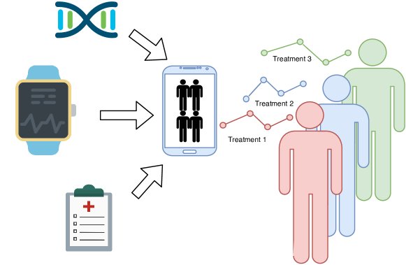
Figure 1: An individual’s genetic, physiological, and clinical data can be used to synthesize their counterfactuals under multiple interventions using donor units.

Randomized Controlled Trials (RCTs) are the current gold standard for evaluating the effect of a treatment. In an RCT, participants are randomly assigned to either an intervention arm or a control arm. The outcome variables of the exposed and control groups are then compared to estimate the treatment effect. This approach is population-based and forces physicians to adopt a one-size-fits-all treatment that is prone to error. Moreover, RCTs raise a variety of issues around ethics and cost [2]. In contrast to traditional population-based methods of evaluating treatments, precision medicine encourages personalized approaches to “delivering the right treatments, at the right time, every time to the right person,” a phrase famously recited by former U.S. President Barack Obama. In the absence of RCTs, social scientists rely on Comparative Case Studies (CCS) to estimate the effect of an intervention. In CCS, a group of ‘donor’ units is collected that resemble the unit of interest prior to the onset of intervention. Then the evolution of the donors produces a counterfactual for the unit of interest. However, finding the donors is empirically driven and the existence of a good match is not guaranteed.

Abadie et al. [3, 4] pioneered a powerful data-driven approach to aggregate observational data from several donor control units to compute the Synthetic Control (SC) of a target unit that receives treatment. They posited that a combination of several unaffected units provides a better match to the affected unit than any unaffected unit alone. Hence, the SC method assigns a non-negative weight to each donor. Such weights sum to 1.0 such that a convex combination of these units best estimates the treated unit prior to the intervention. After that, the post-intervention donor combination yields the desired counterfactual. Prior works have relaxed the convex constraints on the vanilla SC estimator and explored regression-based estimators to compute the assigned weights [5, 6]. Moreover, recent works [7, 8, 9] use matrix estimation methods to make SC more robust to noise and missing data. Similarly, Synthetic Intervention (SI) for a target control unit can be estimated by selecting donor units that undergo the intervention [10]. While SC can generate longitudinal trajectories of patient progress with no intervention exposure, SI can simulate trajectories under a medical intervention. The class of linear SC methods essentially solves an optimization problem for mapping donors to the target across temporal slices using universal, time-agnostic weights. While approaches based on linearly combining donor outcomes to estimate the counterfactual yield an agile model, they overlook both the inter-unit and intra-unit temporal context while making predictions, as illustrated in Fig. 2. These additional relations are essential to take into account because the evolution dynamics of a unit may lead to long-range temporal dependencies that can extend into other units and cause co-movement. We formalize this notion in Section 3.1.

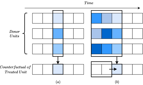
Figure 2: Synthetic control: (a) The vanilla SC method generates control via a convex interpolation of the donors across temporal slices using time-agnostic weights. (b) We view the problem through the lens of a sequence-to-sequence modeling problem and use local spatiotemporal context while predicting control.

In this work, we are interested in the point treatment setting where the counterfactual is estimated after an intervention is administered once to a target unit at some time instance. We recast the problem of counterfactual prediction as a sequence-to-sequence (Seq2Seq) mapping problem where the pre-intervention spatiotemporal context of every unit is mapped into the post-intervention sequence of the target. From a modeling standpoint, we introduce a novel Transformer-based model [11] that uses self-attention to learn complex dynamics. At its core, a Transformer is a generalized differentiable computer that is expressive in the forward pass, easily optimizable via back-propagation, and highly parallel computationally. Thus it can be used as an efficient universal compute engine wrapped around by modality-specific encoder and decoder heads to model diverse modalities simultaneously. Prior counterfactual estimation methods hinge on the provision of simple vector covariates but are unamenable to complex inputs like images and audio, whereas Transformers have shown remarkable modeling properties in these areas. Thus this choice of model opens up the avenue to do counterfactual estimation on all kinds of medical data. In Section 5.4, demonstrate our framework on ubiquitously occurring discrete classes, a simple abstraction that no prior works have tackled. Due to the spatial component of the problem, we modify the decoder attention map to enable bidirectional attention spatially while still maintaining temporal causality. Furthermore, we inject spatial and temporal embeddings to help the model learn the input token order and add an additional target embedding to separate the target and donor units. From a computational perspective, while SC estimates rely on a relatively small number of donors, Transformer models traditionally require large amounts of data to be trained from scratch. To mitigate this problem, we formulate a novel self-supervision-based pre-training task for the Transformer model. The Transformer-based estimator captures rich nonlinear function classes, accounts for irregular observations, and is easy to train using backpropagation. It is, therefore, a practical non-parametric approach for modeling complex real-life data compared to linear SC estimators whose assumption of time-invariant correlation across units fails for weakly coupled dynamical systems. Our experiments show that the model outperforms prior state-of-the-art estimators on synthetic datasets for different donor pool sizes and remains robust to noise. Running ablation studies on the pre-training step reveals that it is critical to learning a good estimator. We study the effectiveness of an anti-tobacco law passed in California and probe the attention layer of the Transformer model to generate a rich description of spatiotemporal donor weights. We also focus on the individual level and model the control counterfactual of patients in a randomized trial on drugs for childhood Asthma. Finally, we simulate synthetic counterfactuals under a Calcitriol supplement intervention for a Friedreich’s ataxia (FA) patient.

2 Related Work

Our work relates most closely to [3] which first introduced the SC method to measure the economic ramifications of terrorism on Basque Country in a panel data setting. They took observational data from other Spanish regions and assigned them convex weights to generate an interpolated SC. They also used their method to analyze the Proposition 99 Excise Tax effect on California’s tobacco consumption [4]. Since then, this method to estimate counterfactuals has gained a lot of popularity and has been used in the social sciences to study legalized prostitution [12], immigration policy [13], taxation [14], organized crime [15], and various other policy evaluations. Other notable works that use regression-based techniques to estimate the control using observed data from other units are the panel data-based estimation method introduced in [5] and the additive-difference-based estimator proposed in [6]. Recently, Robust Synthetic Control (RSC) [7] was proposed as a robust variant of the SC method. It sets up the problem as an unconstrained least squares regression problem with sparsity terms and therefore extrapolates the control from the donors. In addition, the authors introduce a low-rank decomposition denoising step to handle missing data and noise that are ubiquitous in real-world data. Multi-dimensional Robust Synthetic Control (mRSC) [8] extends RSC and proposes an algorithm to incorporate multiple covariates into the model. Ref. [9] poses the synthetic control problem as estimating missing values in a matrix. For an extensive literature review of SC, see [16]. The authors in [17] propose a neural network-based estimator that learns a unit-specific representation and thereafter uses them to find donor weights. The linear SC estimators have been generalized to generate synthetic counterfactuals under any intervention [10]. Most of the above works make the strong parametric assumption that the underlying data-generating process is a linear factorized model of a time-specific and unit-specific latent. Therefore, the proposed models combine donor outcomes across temporal slices and forgo any temporal context. Comparative case studies have been used historically to estimate the control [18, 19]. However, such works have not formalized the selection of the donor pool.

Orthogonal to SC, structural time series methods under the stringent unconfoundedness assumption use temporal regularities across control paths to extrapolate the pre-treatment trajectory to the counterfactual outcome of the treated unit [20, 21, 22]. Structural models need many donor paths and are not amenable to settings like healthcare where the donor pool is small. Difference in Difference (DiD) methods have also been used in healthcare applications [23], but they rely on the strong assumption that the slopes of observed post-treatment units and control units diverge only because of the treatment, such that any difference in slopes can be attributed to the intervention. Thus, non-parallel trends present a major challenge to the validity of this model. Besides, there exists a rich literature on non-SC machine-learning-driven counterfactual estimation. Neural network-based techniques have been used to estimate the Individual Treatment Effect in both static [24, 25] and longitudinal settings [26].

While the importance of disease progression models is widely recognized, there are few works that apply advanced modeling approaches to the task. Many methods use basic statistics and rely on a large amount of domain knowledge. More sophisticated probabilistic or statistical models exist but tend to be exclusively applicable to a specific target disease. Using a more general framework, ref. [27] predicts the stage of chronic obstructive pulmonary disease progression with a graphical model based on the Markov Jump Process. One Transformer model under the broad umbrella of disease progression models has been proposed; [28] predicts the development of knee osteoarthritis with a Transformer model designed for multi-agent decision-making but relies on imaging data. In addition, most neural network approaches to disease progression only predict one to a few metrics of disease, highlighting an area that requires further research.

Many works use neural networks as Seq2Seq models for machine translation using feed-forward networks [29], recurrent neural networks [30], and long short-term memories [31]. Transformer-based models have achieved state-of-the-art results on tasks that span natural language processing (NLP) [11] and, more recently, computer vision [32]. They are pre-trained on large corpora and then fine-tuned for a specific task, with the most notable works being BERT [33], which uses self-supervision-based denoising tasks, and GPT [34, 35], which uses a language-modeling-based pre-training task. Our work adds to these works by proposing a model to map spatiotemporal data and introducing a self-supervision-based pre-training task that supports the mapping.

3 Background

In this section, we outline the key assumptions and formally set up the problem of generating synthetic counterfactuals using donor units.

3.1 Assumptions

The problem consists of a ‘target’ unit and $\mathit{N}$ ‘donor’ units with $\mathit{N}$ typically small. A unit can refer to an aggregate of a population segment or an individual. $\mathit{N}$ donor units undergo the intervention we are interested in at the same time instance. Without loss of generality, we assume that control assignment is also a type of intervention and finding the counterfactual under control reduces to the SC problem. For each unit, panel data are available for a time period $\mathit{T}\;$ and the covariate in each panel can have missing data. We make standard assumptions about the units.

1. Stable Unit Treatment Value Assumption (SUTVA): The potential outcomes for any unit do not vary with the treatments assigned to other units and, therefore, there are no spillover effects.

2. No anticipation of treatment: This implies that the units cannot anticipate the assignment of treatment a priori and, therefore, the assignment has no effect on the pre-intervention trajectory.

3. Exchangeability (No unmeasured confounders): This assumption implies that units that are exposed and unexposed have the same potential outcomes on average and hence in the case of an observational study, a control group can be reliably used to measure the counterfactual of the treatment group.

4. Positivity (Common support): This necessitates covariates in the control and the treatment group have overlapping distributions (common support), in the absence of which it is impossible to understand the causal effect of a treatment because a subset of the population is always entirely left treated or untreated.

Data-generation Process: The underlying data generation of a unit $i$ consists of unit-specific latent $\theta_{i}$ and time-indexed latents $\rho_{t}$. The observation of all covariates of unit $i$ at time $t$, $y_{it}$, depends on all prior temporal latents and is given by:

$$y_{it}=m_{it}+\epsilon_{it},\epsilon_{it}\sim\mathcal{N}(0,\sigma^{2}).$$ (1)

$$m_{it}=f(\theta_{i},\rho_{t},\cdots,\rho_{1}).$$ (2)

Function $f$ is implicitly learned by the Transformer that can capture a wide class of nonlinear autoregressive dynamics. This generalized model that subsumes the models popularly assumed in the literature. Ref. [3] assumes the following model for the data-generation process.

$$y_{it}={\rho_{t}}^{T}X_{i}+\epsilon_{it}.$$ (3)

Here, $\rho_{t}$ denotes the latent at time $t$ and $X_{i}$ denotes the observed covariates of unit $i$. Setting $f$ to the linear factor function and $\theta_{i}=X_{i}$ in Eq. (2) yields the model defined by Eq. (4). Similarly, ref. [17] assumes that:

$$y_{it}={\rho_{t}}^{T}C_{i}+\epsilon_{it}.$$ (4)

where $C_{i}$ is a latent unit-specific representation. It is straightforward to see that Eq. (2) captures this model as well. Refs. [7, 8] assume a non-autoregressive, nonlinear $f$ that is once again a special case of our assumption. Next, we set up the problem formally.

3.2 Problem Setup

The synthetic counterfactual problem uses a ‘target’ unit and $\mathit{N}$ ‘donor’ units. For the SC, the target unit $\mathit{Y}$ is exposed to a treatment or intervention, and the donor units are assumed to be unexposed and, therefore, natural controls. Therefore, we are interested in the counterfactual of the target under the control assignment. On the contrary, donors are exposed to the intervention at a time instance and are natural controls prior to that instance for computing the SI. Therefore, SC and SI are dual problems and simply differ in the type of intervention the donors receive at the intervention instance.

Each unit is $\mathit{T}$ time units long, and at each time step, the sequence has $\mathit{K}$ covariates, e.g., Gross Domestic Product, literacy rate, or physiological data, where each covariate may have missing values. Let each element in the target sequence $Y\in\mathbb{R}^{T\times K}$ be denoted by $y^{t,k}$, where $\mathit{t}$ denotes the time instance and $k$ denotes the covariate. Without loss of generality, assume that the covariate of interest is at $k=1$, and let $\mathit{T_{0}}$ be the time of intervention. The target sequence $Y=[Y^{-},Y^{+}]$ is thus divided into a pre-intervention sequence $\mathit{Y^{-}}\in\mathbb{R}^{T_{0}\times K}$ and a post-intervention sequence $\mathit{Y^{+}}\in\mathbb{R}^{(T-T_{0})\times K}$. Let the tensor $X\in\mathbb{R}^{N\times T\times K}$ represent the data from $\mathit{N}$ donor units and $x^{i,t,k}$ represent each element of the donor tensor $X$, where $i$ is the donor, $t$ is the time instance, and $k$ is the covariate. Let $X=[X^{-},X^{+}]$, where $X^{-}\in\mathbb{R}^{N\times T_{0}\times K}$ and $X^{+}\in\mathbb{R}^{N\times(T-T_{0})\times K}$ denote the pre-intervention and post-intervention data of the donors, respectively. The SC problem involves learning a predictor $f^{t}_{\theta}(.)$ for the post-intervention control of the covariate of interest, $\widehat{y}^{t,1}\;\forall t\in[T_{0}+1,\cdots,T]$, using the donor data $X$ and the pre-intervention target sequence $Y^{-}$. More formally:

$$\widehat{y}^{t,1}=f^{t}_{\theta}\left(X,Y^{-}\right),\>\forall t\in[T_{0}+1,\cdots,T].$$ (5)

3.3 Transformers

Transformers [11] were proposed to model sequential data. They have achieved state-of-the-art results on several NLP tasks. The model consists of stacked layers, where each layer has a self-attention module followed by a feedforward module, and each module has residual connections [36] and layer normalization [37]. The self-attention module learns powerful internal representations that capture important semantic and syntactic associations across input tokens [38]. This module decomposes each token into a query ($Q$), key ($K$), and value ($V$) vector, and uses these vectors to aggregate global information at each sequence position. For finer details of this architecture, we refer readers to the original article.

3.4 Benchmarks

In this section, we describe prior methods to estimate counterfactuals for longitudinal outcomes under a point treatment setting. Since the introduction of the SC technique [3], several modifications to it have been proposed. We describe several state-of-the-art estimators that we benchmark our method against.

3.4.1 Robust Synthetic Control (RSC)

The RSC method [7] assumes a linear model and introduces a denoising step to the SC method. Furthermore, it uses regularized regression to find the optimal weights $\beta^{*}$. Let $\hat{p}$ be the fraction of missing data in $X$. The authors replace missing data in $X$ with $0$ and estimate a low-rank matrix $\hat{M}$ from $X$ as follows:

$$X=\sum s_{i}u_{i}v_{i}^{T}.$$ (6)

$$S=\{i:s_{i}\geq\mu\}.$$ (7)

$$\hat{M}=\frac{\sum_{i\in S}s_{i}u_{i}v_{i}^{T}}{\max(1-\hat{p},\frac{1}{NT})}.$$ (8)

The threshold $\mu$ above is a hyperparameter. Let $\hat{M}=[\hat{M}^{-},\hat{M}^{+}]$, where $\hat{M}^{-}$ and $\hat{M}^{+}$ denote the pre-intervention and post-intervention data, respectively. The optimal weights $\beta^{*}$ are computed using the LASSO regularized regression as follows:

$$\beta^{*}=\operatorname*{arg\,min}_{\beta}\left\lVert Y^{-}-M^{-T}\beta\right\rVert^{2}+\eta\left\lVert\beta\right\rVert_{1}.$$ (9)

The counterfactual is predicted through

$$\widehat{Y}=\hat{M}^{+T}\beta^{*}.$$ (10)

3.4.2 Multi-Dimensional Robust Synthetic Control (mRSC)

The same authors [8] generalize RSC to incorporate multiple additional covariates to predict the covariate of interest. At a high level, they flatten their donor tensor $X\in\mathbb{R}^{N\times T\times K}$ to a matrix $Z\in\mathbb{R}^{N\times KT}$. After that, they run the denoising step from RSC on $Z$ and perform a covariate-based re-weighting on the resultant low-rank matrix and target matrix $Y$. In their final step, they run regression on the pre-intervention data of the re-weighted matrices.

3.4.3 Matrix Completion using Nuclear Norm Minimization (MC-NNM)

The authors in [9] estimate the counterfactual by treating them as missing values of a matrix. Let $Y\in\mathbb{R}^{T\times(N+1)}$ denote the outcome matrix of the donor and target units. Then the underlying structure assumed on the matrix $Y$ by the authors is:

$$Y=L^{*}+\epsilon$$ (11)

$$L^{*}=\hat{L}+\hat{\tau}\mathbf{1}_{T}^{T}+\mathbf{1}_{N}\hat{\Delta}^{T}$$ (12)

Here $L^{*}$ denotes the true mean matrix, $\hat{\tau}$ models the fixed temporal effect, $\hat{\Delta}$ accounts for the unit wide fixed effect and $\mathbf{1}$ indicates a vector of ones. Thereafter, the true matrix $L^{*}$ is recovered by setting up the following optimization problem with a penalty on the nuclear norm.

$$(\hat{L},\hat{\tau},\hat{\Delta})=\operatorname*{arg\,min}_{L,\tau,\Delta}\lVert Y-L-\tau\mathbf{1}_{T}^{T}-\mathbf{1}_{N}\Delta^{T}\rVert_{F}+\lambda\lVert L\rVert$$ (13)

3.4.4 Sync-Twin

The authors in [17] propose a learning algorithm to learn a deep representation $c_{i}$ for the units using pre-intervention covariates. They assume the following factorised data-generation model:

$$Y_{it}=q_{t}^{T}c_{i}+\epsilon_{it}$$ (14)

where $q_{t}$ denotes the temporal factors. Thereafter, $c_{i}$ is learned by setting up the following reconstruction task over the covariates

$$\hat{c_{i}}=argmin_{c_{i}}\lVert(\tilde{X}_{i}-X_{i})\odot M\rVert$$ (15)

Here, $M$ is a mask for missing covariates. Since the underlying model is linear in $\hat{c}_{i}$, the donor weights are calculated by regressing in the representation space $C$:

$$\beta^{*}=\operatorname*{arg\,min}_{\beta}\left\lVert c_{treated}-\hat{C}^{T}\beta\right\rVert^{2}$$ (16)

4 Spatiotemporal Seq2Seq Modeling

In our work, we view the problem through the lens of Seq2Seq modeling. For the intervention instance $T_{0}$, we denote the counterfactual of the target until time $t$ as $\hat{Y}^{t}=[\hat{y}^{T_{0}},\hat{y}^{T_{0}+1},\cdots,\hat{y}^{t}]$ and similarly the post-intervention of the donor data until $t$ as $X^{+t}\in\mathbb{R}^{N\times(t-T_{0})\times K}$. Then we model the distribution of the synthetic counterfactual as:

$$P(\hat{Y}|X,Y^{-})=\prod_{t=T_{0}+1}^{T}P_{\theta}(\hat{y}^{t}|\hat{Y}^{t-1},X^{+t},X^{-},Y^{-}).$$ (17)

We use an encoder-decoder model, where the encoder $f_{\alpha}(.)$ computes a hidden representation $\mathcal{V}$ for the pre-intervention data $\langle Y^{-},X^{-}\rangle$ and passes it to the decoder $g_{\phi}(.)$ that uses the representation and the post-intervention donor data $X^{+t}$ to autoregressively generate the control $\hat{y}^{t}$.

$$\mathcal{V}=f_{\alpha}(X^{-},Y^{-}).$$ (18)

$$P_{\theta}(\hat{y}^{t}|\hat{Y}^{t-1},X^{+t},X^{-},Y^{-})=g_{\phi}(\hat{Y}^{t-1},X^{+t},\mathcal{V}).$$ (19)

4.1 Architecture

An overview of our Transformer model is given in Fig. 3. It encodes pre-intervention data of temporal length $l^{-}$ and decodes it into post-intervention data of temporal context $l^{+}$. The pre-intervention data of the target and the donors can be represented by the tensor $Z^{-}=[Y^{-};X^{-}]\in\mathbb{R}^{(N+1)\times l^{-}\times K}$. Similarly, the post-intervention data are represented by $Z^{+}=[\hat{Y};X^{+}]\in\mathbb{R}^{(N+1)\times l^{+}\times K}$. The standard Transformer receives a 1D sequence of input tokens. Hence, we flatten $Z^{-}$ and $Z^{+}$ into a 1D sequence $Z_{flat}^{-}\in\mathbb{R}^{(N+1)l^{-}\times K}$ and $Z_{flat}^{+}\in\mathbb{R}^{(N+1)l^{+}\times K}$, respectively. We then project each token into the hidden dimension $D$ of the Transformer via a trainable linear weight $W_{e}\in\mathbb{R}^{K\times D}$ to give sequences $E^{-}\in\mathbb{R}^{(N+1)l^{-}\times D}$ and $E^{+}\in\mathbb{R}^{(N+1)l^{+}\times D}$. More precisely,

$$E^{-} =Z^{-}_{flat}W_{e}=\left[x^{i,t}W_{e};\cdots x^{N,t}W_{e};y^{-t}W_{e}\right]_{t=T_{0}-l^{-}+1}^{T_{0}}.$$ (20)

$$E^{+} =Z^{+}_{flat}W_{e}=\left[x^{i,t}W_{e};\cdots x^{N,t}W_{e};\hat{y}^{t}W_{e}\right]_{t=T_{0}+1}^{T_{0}+l^{+}}.$$ (21)

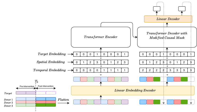
Figure 3: An overview of our model. We flatten the pre-intervention and post-intervention data into sequences and linearly embed them. Next, we add positional information in the form of temporal and spatial embeddings, and help the model differentiate between the target and donor units by injecting a target embedding. The resultant sequence of vectors is fed to the Transformer-based encoder-decoder model. The decoder uses a modified causal map, which enables spatial bidirectionality, to autoregressively generate SC of the treated unit.

4.1.1 Positional and Target Embeddings

Each token in the sequence belongs to one of $N+1$ tokens, one of $T$ time instances, and either a donor or the target unit. We, therefore, inject a learnable spatial embedding $\mathbb{E}_{spatial}(.)\in\mathbb{R}^{(N+1)\times D}$, time embedding $\mathbb{E}_{t}(.)\in\mathbb{R}^{T\times D}$, and a target embedding $\mathbb{E}_{target}(.)\in\mathbb{R}^{2\times D}$ to enable the model to differentiate between spatiotemporal positions of the token in the data matrix as well as separate donors from the target unit. The resultant encoder input $\mathit{H^{-}}$ and the decoder input $\mathit{H^{+}}$ sequences are obtained as follows:

$$H^{-}=E^{-}+\mathbb{E}_{spatial}(E^{-})+\mathbb{E}_{t}(E^{-})+\mathbb{E}_{target}(E^{-}).$$ (22)

$$H^{+}=E^{+}+\mathbb{E}_{spatial}(E^{+})+\mathbb{E}_{t}(E^{+})+\mathbb{E}_{target}(E^{+}).$$ (23)

4.1.2 Encoder

We use the vanilla bidirectional Transformer encoder with a latent dimension $\mathit{D}$ consisting of $l$ stacked identical layers. The encoder processes the input sequence $H^{-}$ and outputs a sequence of representations $\mathcal{V}$ over the input. A key $K$ and value $V$ vector are computed over each of the tokens in $\mathcal{V}$ and passed to the decoder.

4.1.3 Decoder

The decoder is tasked with autoregressively generating the counterfactual $\hat{Y}$, given the encoder output $\mathcal{V}$ and sequence $H^{+}$. Our decoder design mostly follows the vanilla Transformer decoder with $l$ stacked identical layers. Each layer has two kinds of attention, viz., causal self-attention module that operates over the decoder hidden states and the ‘encoder-decoder’ attention module that operates over the joint representation of the encoder and decoder. However, we do modify the causal attention mask used in the self-attention module to account for the tokens that lie on the same temporal slice but differ spatially. In other words, we enforce temporal causality but allow bidirectionality spatially. The modified causal mask for spatiotemporal data is illustrated in Fig. 4. We then project the hidden state of SC via a linear weight $W_{d}\in\mathbb{R}^{D\times 1}$ to obtain the prediction.

Algorithm 1 lays out the skeleton of our model.

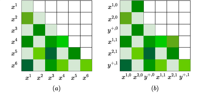
Figure 4: Comparison of the Vanilla decoder mask: (a) that enforces temporal causality and modified causal mask, and (b) that additionally allows spatial bidirectionality.

Algorithm 1 Transformer $(X^{-},X^{+},Y^{-},Y^{+})\rightarrow\hat{Y}$

  Require: $Encoder_{\alpha}$, $Decoder_{\phi}$, $W_{e}$, $W_{d}$, $\mathbb{E}_{spatial}$, $\mathbb{E}_{t}$, $\mathbb{E}_{target}$

  $Z^{-}_{flat}=flatten\left(concat\left(X^{-},Y^{-}\right)\right)$ $\triangleright$ $(N+1)l^{-}\times K$

  $Z^{+}_{flat}=flatten\left(concat\left(X^{+},Y^{+}\right)\right)$$\triangleright$ $(N+1)l^{+}\times K$

  $E^{-}=Z^{-}_{flat}W_{e}$ $\triangleright$ $(N+1)l^{-}\times D$

  $E^{+}=Z^{+}_{flat}W_{e}$ $\triangleright$ $(N+1)l^{+}\times D$

  $H^{-}=E^{-}+\mathbb{E}_{spatial}(E^{-})+\mathbb{E}_{t}(E^{-})+\mathbb{E}_{target}(E^{-})$

  $H^{+}=E^{+}+\mathbb{E}_{spatial}(E^{+})+\mathbb{E}_{t}(E^{+})+\mathbb{E}_{target}(E^{+})$

  $\mathcal{V}=Encoder_{\alpha}(H^{-})$

  $Z=Decoder_{\phi}(H^{+},\mathcal{V})$

  $\hat{Z}=Z.target$ $\triangleright$ Target Hidden States

  $\hat{Y}=\hat{Z}W_{d}$ $\triangleright$ $l^{+}\times K$

  return $\hat{Y}$

4.2 Data Preprocessing

We replace missing data with $0$ and scale each covariate in the data between $0$ and $1$ before processing by the Transformer. Motivated by mRSC [8], we apply a low-rank transformation to the data tensor $X\in\mathbb{R}^{N\times T\times K}$ when data are missing. We flatten $X$ to $X_{flat}\in\mathbb{R}^{N\times TK}$ and retain the top $m$ singular values of $X_{flat}$.

4.3 Pseudo-Counterfactual Prediction Pre-training

Transformer-based language models are usually pre-trained on an unsupervised task [33, 34] to learn high-capacity representations that help boost downstream performance on discrimination tasks. In the same way, we pre-train the model on donor data to reliably reconstruct the counterfactual, the ground truth of which is known. In each training iteration, we sample a donor unit $X_{i}\in\mathbb{R}^{1\times T\times K},i\in[1,\cdots,N]$ and an intervention time $T^{\prime}\in[1,\cdots,T]$. We treat the sampled donor as a pseudo-target and task our model with generating its post-intervention counterfactual. Let $X_{\backslash i}^{-}\in\mathbb{R}^{(N-1)\times l^{-}\times K}$ and $X_{\backslash i}^{+}\in\mathbb{R}^{(N-1)\times l^{+}\times K}$ denote the pre-intervention and post-intervention donor data excluding the sampled donor, respectively, and let $\hat{X}_{i}^{t}\in\mathbb{R}^{(N-1)\times(t-T^{\prime})\times K}$ denote the post-intervention control of the pseudo-target until time $t$ and $\hat{x}_{i}^{t}$ be the control at instance $t$. The objective of the model is to maximize the following log-likelihood:

$$\mathcal{L}(\alpha,\phi)=\sum_{t=T^{\prime}+1}^{T^{\prime}+l^{+}}log(P(\hat{x}_{i}^{t}|\hat{X}_{i}^{t-1},X_{\backslash i}^{+t},X^{-},\alpha,\phi))$$ (24)

We use the teacher forcing algorithm [39] while training and assume a Gaussian model for the likelihood that reduces the loss function to squared error.

4.4 Fine-tuning

Fine-tuning proceeds by fitting the model on the pre-intervention data $Y^{-}$ of the target unit using the pre-intervention donor data $X^{-}$. In each fine-tuning iteration, we sample a time instance $T^{\prime}$ in $[1,\cdots,T_{0}]$ for use as the pseudo-intervention instance. Then, we treat $X^{-}$ and $Y^{-}$ as the data in hand and divide it into pseudo-pre-intervention and pseudo-post-intervention data to predict the pseudo-post-intervention of the target.

4.5 Inference

We generate the SC $\hat{Y}$ in a sliding window fashion, where we start at $T_{0}$ and generate post-intervention data of temporal length $l^{+}$ each time. The generated control is used as pre-intervention data for the subsequent time steps. Algorithm 2 shows the pseudo-code for training and inference.

Algorithm 2 Training and Inference

  Require: Transformer($\alpha,\phi$), Learning rate $\lambda$

  $\triangleright$ Pre-training($X$, $iters$)

  for $j=1$ to $iters$ do

     $i=random.sample(N)$

     $T_{0}=random.sample(T)$

     $Y\;=\;X[i]$ $\triangleright$ Pseudo Target

     $X^{\prime}\;=\;X.remove(i)$$\triangleright$ Pseudo Donor

     $Y^{-},\;Y^{+}=\;Y\;[T_{0}-l^{-}:T_{0}],\;Y\;[T_{0}:T_{0}+l^{+}]$

     $X^{-},\;X^{+}=X^{\prime}[:,T_{0}-l^{-}:T_{0}],\;X^{\prime}[:,T_{0}:T_{0}+l^{+}]$

     $preds$ = Transformer($X^{-},X^{+},Y^{-},Y^{+}$)

     $\mathcal{L}$ = $mean\left((Y^{+}-preds)^{2}\right)$

     $\alpha\leftarrow\alpha-\lambda\nabla_{\alpha}\mathcal{L},\;\phi\leftarrow\phi-\lambda\nabla_{\phi}\mathcal{L}$

  end for

  $\triangleright$ Fine-tuning($X,Y,T_{0}$, iters)

  for $j=1$ to $iters$ do

     $T^{\prime}=random.sample(T_{0})$

     $Y^{\prime}\;=\;Y\;[:T_{0}]$

     $X^{\prime}\;=\;X\;[:,:T_{0}]$

     $Y^{-},\;Y^{+}=\;Y^{\prime}\;[T^{\prime}-l^{-}:T^{\prime}],\;Y^{\prime}\;[T^{\prime}:T^{\prime}+l^{+}]$

     $X^{-},\;X^{+}=X^{\prime}[:,T^{\prime}-l^{-}:T^{\prime}],\;X^{\prime}[:,T^{\prime}:T^{\prime}+l^{+}]$

     $preds$ = Transformer($X^{-},X^{+},Y^{-},Y^{+}$)

     $\mathcal{L}$ = $mean\left((Y^{+}-preds)^{2}\right)$

     $\alpha\leftarrow\alpha-\lambda\nabla_{\alpha}\mathcal{L},\;\phi\leftarrow\phi-\lambda\nabla_{\phi}\mathcal{L}$

  end for

  $\triangleright$ Inference($X,Y^{-},T_{0}$) $\rightarrow\hat{Y}$

  $X^{-}\;=\;X\;[:,T_{0}-L^{-}:T_{0}]$

  $\hat{Y}$ = [ ]

  for $I=1$ to $l^{+}$ do

     $X^{+}\;=\;X\;[:,T_{0}:T_{0}+i]$

     $preds$ = Transformer($X^{-},X^{+},Y^{-},\hat{Y}$)

     $\hat{Y}=\hat{Y}.append(preds[i])$

  end for

  return $\hat{Y}$

4.6 Visualization

A key property of the simple linear model assumed by the vanilla SC method is its interpretability in the form of donor weights. Modeling the spatiotemporal context helps us visualize the donor contributions across different time instances. Transformers are effective at long range credit assignment and the attention score $a_{ij}$ in the attention matrix $A$ of the Transformer specifies the proportion with which a token $i$ attends to token $j$. We probe the self-attention layers of the decoder and extract the attention scores of various donors while predicting the target token. While not entirely dispositive of the donor significance, this can help domain experts uncover the relations between targets and important donors.

We qualitatively compare our proposed approach against prior techniques in Table 1 with respect to four features. 1) Nonlinearity: Whether the model captures nonlinear dynamics. 2) Missing Data: Whether the proposed algorithm considers missing data values for the outcome variable and covariates. 3) Temporal Context: Whether the model implicitly or explicitly considers the prior context. 4) Multimodal Inputs: Whether multimodal data like images, audio, and discrete classes can be processed by the proposed approach.

Table 1: Qualitative comparison of past approaches and our method. ✓  indicates the presence of a feature and ✗  denotes its absence. *Sync Twin only considers missing pre-intervention covariates.

Method	Non Linearity	Missing Data	Temporal Context	Multimodal Inputs
Synthetic Control [3]	✗	✗	✗	✗
RSC [7]	✗	✓	✗	✗
mRSC [8]	✗	✓	✗	✗
MC-NNM [9]	✗	✓	✓	✗
Sync-Twin [17]	✓	✗*	✗	✗
Spatiotemporal Transformer (Ours)	✓	✓	✓	✓

5 Experiments

We demonstrate the efficacy of our method through quantitative and qualitative experiments. We give the training details, additional results and hyperparameters for each experiment in the Appendix.

5.1 Synthetic Data

Counterfactual estimators are difficult to evaluate on real-life data since the ground truth counterfactual is unknown. Hence, we benchmark our method on synthetic data where the underlying data-generation process is known a priori. We set up an SC problem here by constraining the donors to be controls. The ‘mean’ synthetic data $M$ is generated using a latent factor model. $M\in\mathbb{R}^{(N+1)\times T\times 2}$ has two covariates and the first row represents the target data with the remaining tensor representing donor data. Each row $i$ and column $j$ is assigned a latent factor $\theta_{i}$ and $\rho_{j}$, respectively, and covariate $k$ is generated using $f_{k}(\theta_{i},\rho_{j})$. We use

$$\begin{split}f_{1}(\theta_{i},\rho_{j})=\theta_{i}+\frac{(\rho_{j}\times\theta_{i})}{T}exp(\frac{\rho_{j}}{T})+cos(2\mathcal{F}_{1}\frac{\pi}{180})+\\ sin(\mathcal{F}_{1}\frac{\pi}{180})+cos(2\mathcal{F}_{2}\frac{\pi}{180})+sin(\mathcal{F}_{2}\frac{\pi}{180}).\end{split}$$ (25)

$$f_{2}(\theta_{i},\rho_{j})=\frac{10}{1+exp(-\theta_{i}-\frac{\rho_{j}}{T}-0.7\frac{\theta_{i}\rho_{j}}{T})}.$$ (26)

Here, $\mathcal{F}_{1}=(\rho_{j}\;mod\;360),\;\mathcal{F}_{2}=(\rho_{j}\;mod\;180)$. Thereafter, we add noise $\epsilon\sim N(0,\sigma^{2})$ to each entry in $M$ to obtain the observed matrix $O$. Given an intervention instance $T_{0}$, we task the estimator to reconstruct the post-intervention ($t>T_{0}$) mean sequence of the first covariate from noisy observations. Note that our data-generation process is similar to [8] with the critical distinction being that the mean target sequences are generated from a high-rank latent factor model instead of being linearly extrapolated from donor units composed from a low-rank latent factor model. This makes the task inherently ‘harder’. For all the experiments run on synthetic data, we set $T=2000,\;T_{0}=1600,\;\rho_{j}=j$, and $\theta_{i}$ is uniformly sampled from $[0,1]$. Our proposed method is compared against all the benchmark methods mentioned in Section 3.4, using the root mean squared error (RMSE) between the estimates and the true post-intervention mean. In addition, to this we also learn a simple Transformer based decoder baseline to perform time series modeling on the donor trajectories. This baseline therefore corresponds to the extreme case of zero donors used to extrapolate the counterfactual under the modeling framework.

5.1.1 Robustness against Noise

Next, we investigate the robustness of our method against noise in the observed data. We set $N=10$ and generate three synthetic datasets with varying noise levels $\sigma^{2}\in[0.5,\;1,\;2]$. The RMSE scores are reported in Fig. 5 and Fig. 6 shows the synthetic control estimates. The Transformer baseline performs the worst, which is expected given traditional transformers’ data inefficiency. This also indicates the difficulty of using simple time series extrapolation with few donors and shows the benefits of directly modeling the donor outcomes to perform few-shot counterfactual estimation. As noise increases, our predictions remain robust and lie close to the true mean without using any denoising step. Moreover, pre-training is essential for helping our model learn a useful representation of the underlying latent model, thus in making accurate predictions.

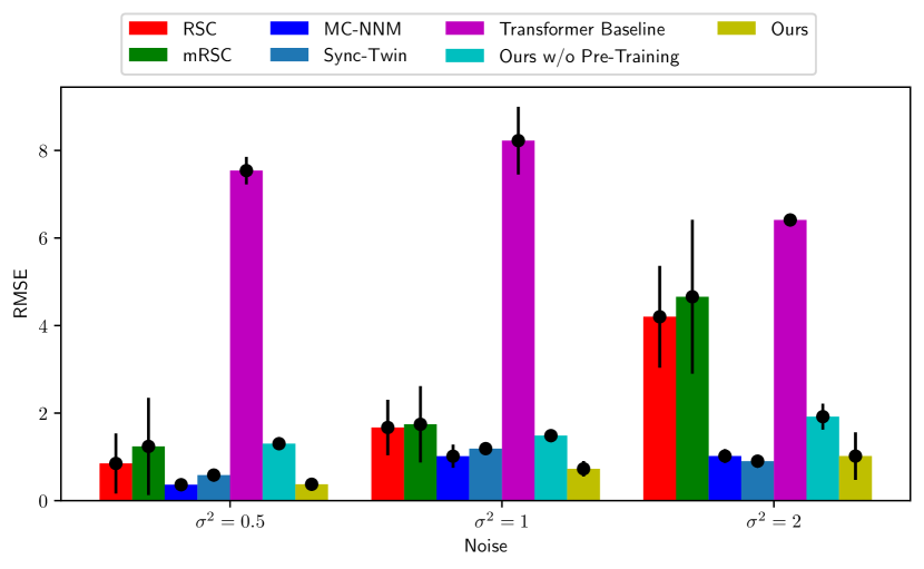
Figure 5: Comparison between post-intervention RMSE of our approach and prior estimators using observations with varying noise levels. Our approach surpasses or performs at par with these techniques at all levels of noise. Moreover using donors and therefore spatiotemporal transformers (yellow) gives $\mathbf{6x-20x}$ reduction in error over simple temporal modeling of control path using Transformers (purple). Error bars are plotted at 90% confidence intervals.

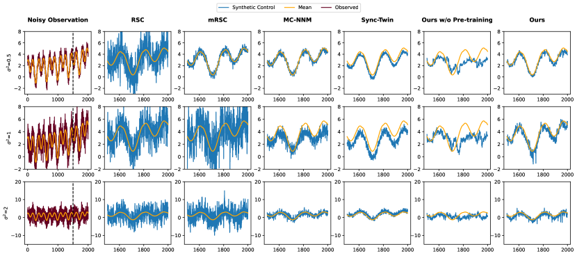
Figure 6: Estimates of the post-intervention mean of the target from noisy observations for $N=10$ and varying levels of noise. The vertical black line indicates the intervention instance.

5.1.2 Effect of the donor pool size

From Fig. 7, we gain insight into the effect of the donor pool size on the accuracy of our prediction. Synthetic counterfactual problems often tend to have a small number of donors for eg. few states tend to experience similar policies, rare diseases inflict a small number of the population etc. Hence, we set $N\in[5,10,15,25,50,75,100]$ with $\sigma^{2}=1$. Our estimator achieves a lower RMSE for most donor pool sizes with pre-training. We plot the SC estimates obtained by all the evaluated methods for different donor pool sizes in Fig. 8. Note that, the performance without pre-training the model is worse and, therefore, this step is crucial for the model to be biased in the right way prior to finetuning. For $N=5$, we observe that our model underfits compared to other methods. This is expected given the complexity of Transformer models and the data constraints for extremely few number of donors. However we outperform the other models as the number of donors increase. With the availability of more donors, the performance margin between linear estimators and our model narrows. We attribute this observation to two causes. First, we posit that the other models, which assume underlying linear factorized models with fixed temporal effects, need a higher number of donors to control for time-varying confounders and hence yield better predictions only when the donors increase. Second, the stronger choice of inductive bias by using all the donors simultaneously to predict the outcomes leads to slight overfitting for spatiotemporal transformers as the number of donors increase. This opens up interesting directions to prevent such overfitting via prior donor elimination, sparsity constraints on Transformer attention among other possible regularization methods and we leave this for future work.

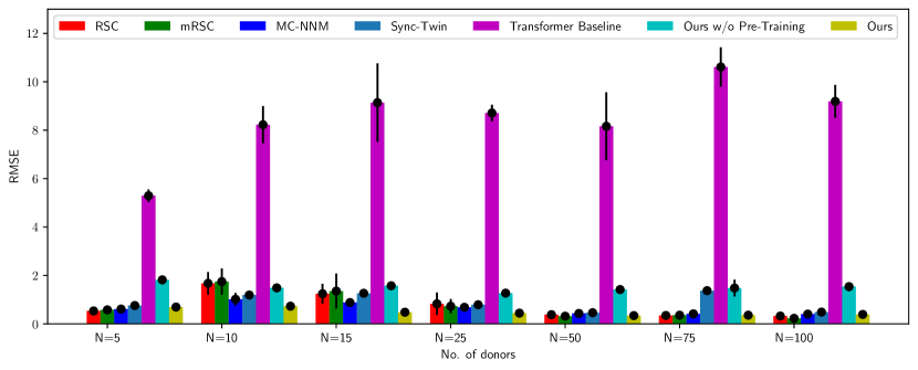
Figure 7: Post-intervention RMSE of various estimators with varying donor pool size. Our approach performs competitively for most donor pool sizes with the pre-training step being crucial to achieving an accurate prediction. Using spatiotemporal transformers (yellow) reduces error over a traditional Transformer (purple) by $\mathbf{6x-19x}$. Plotted at 90% confidence intervals.

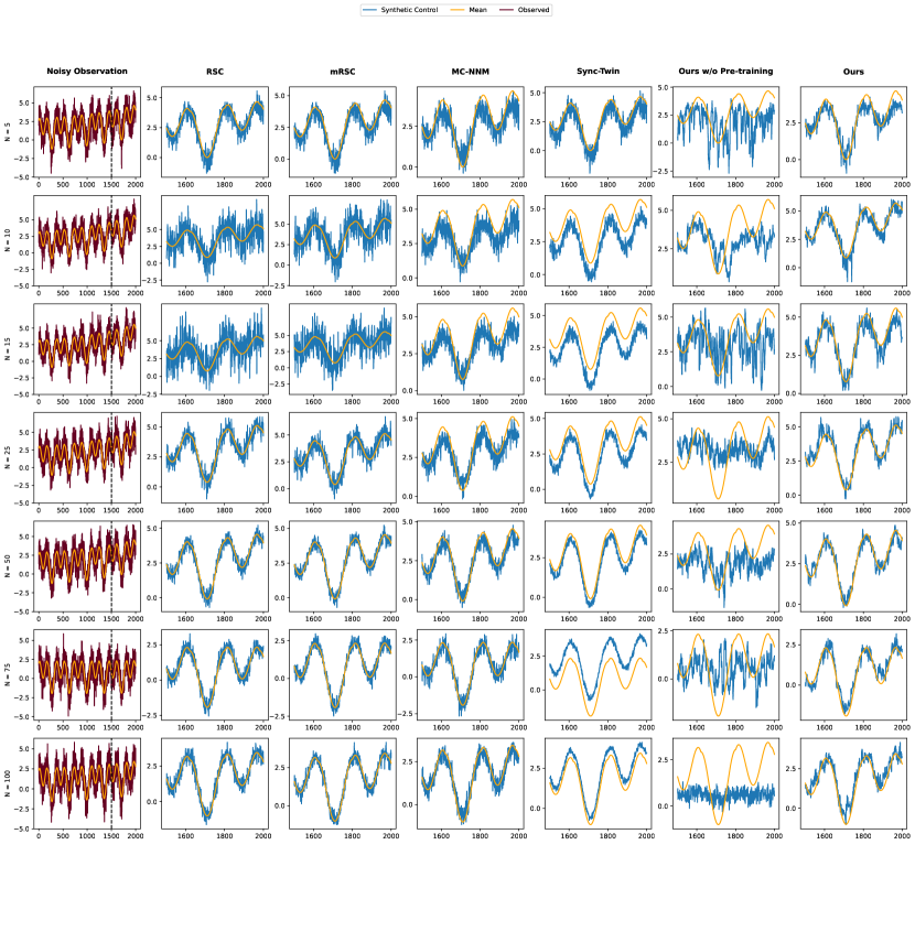
Figure 8: Effect of donor pool size on SC estimates. Our approach surpasses or performs competitively with prior estimators for all donor sizes in consideration

Next, we evaluate our approach on real-life datasets at both population and individual levels spanning public health, randomized trials, and rare diseases.

5.2 Analysing Public Health Policy: California Proposition 99

In 1988, California became the first in the United States to pass a large anti-tobacco law, Proposition 99, that hiked the excise tax on cigarette sales by 25 cents. To evaluate the effectiveness of this law, we construct a synthetic California without Proposition 99 and measure the per capita cigarette sales in this synthetic unit. The donor pool consists of 38 control states where no significant policies for tobacco control were introduced and additional covariates like beer consumption, population, and income are included. Fig. 9 compares the California counterfactual prediction of our method and various baselines, all showing that the cigarette sales would have been higher in the absence of the law. We infer that per-capita cigarette sales fell by 45 packets in real California towards the year 2000 compared to synthetic California. Moreover, our model makes the intuitive prediction that in the absence of the law, cigarette sales in California would converge to the national average. As explained in Section 4.6, attention scores of the model can be used to extract the contribution of the donors in making the counterfactual prediction. These weights across the donor space and time are illustrated in Fig. 10, indicating the combination that best reproduces the outcome before the passage of Proposition 99.

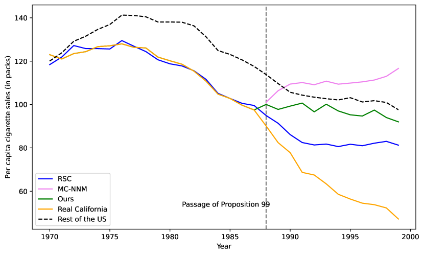
Figure 9: Comparison of methods on synthetic vs. true California. We infer that the passage of Proposition 99 reduced per-capita cigarette sales from the gap between observed California (yellow) and the synthetic counterfactual of California (green). Our model also predicts that in the absence of Proposition 99, cigarette sales in California would slowly converge to the national average (dotted line).

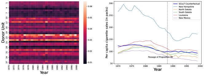
(a) Layer 1 spatiotemporal donor attention

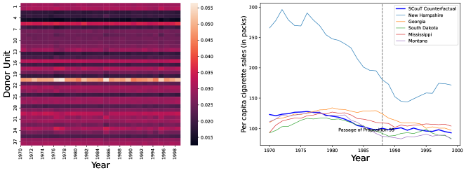
(b) Layer 2 spatiotemporal donor attention

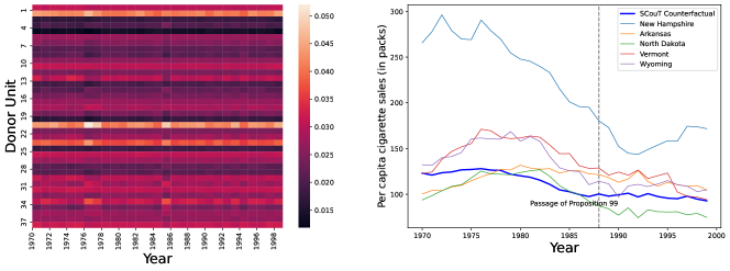
(c) Layer 3 spatiotemporal donor attention

Figure 10: Figures (a), (b), (c) on the left visualize donor attentions for the three layers of the Transformer. Attention is sparse and spread across specific donors, with the sparsity becoming more pronounced in the deeper layers. For each attention distribution map, we extract top 5 donors and plot them against our synthetic counterfactual on the right. We note that New Hampshire that has highest cigarette sale per capita among all the states is consistently used across all attention layers. On the other hand, the model selects specific donors at every layer to iteratively refine its counterfactual.

5.3 SCouT for Insilico Randomized Trails: Drug trials for Childhood Asthma

At the patient level, the synthetic counterfactual is a dynamic, virtual representation of the human being over time and enables applications for in silico clinical trials. As an example, we look at The Childhood Asthma Management Program (CAMP) [40], an RCT designed to study the long-term pulmonary effects of three treatments (budesonide, nedocromil, and placebo) on children with mild-to-moderate asthma. The trial’s placebo arm contains anonymized longitudinal data of 275 patients with over 20 spirometry measurements per patient. Pre-Bronchodilator Forced Expiratory Volume to Forced Vital Capacity ratio (PreFF) is a vital metric of lung capacity in Asthma patients that measures volume of air that an individual can exhale during a forced breath prior to the usage of a bronchodilator. Here, we model the control arm of the RCT and predict the PreFF of a target patient using the other placebos as donors. We consider two settings, where pre-intervention lengths are 35% and 75% of the total trajectory. One at a time, we set one patient as the target unit and consider the others as donors. In this fashion, we model the control paths of the first five patients in the placebo arm, the ground truths available to us. The average RMSE across these patients is reported in Fig. 11. We plot the counterfactual estimates for patients in Fig. 12. Our method generates a reliable control along with MC-NNM whereas estimates produced by RSC and mRSC are highly biased. We posit that local spatiotemporal mapping is reasonably effective in controlling for time-dependent confounders, whereas linear estimators that assign time-agnostic weights suffer significantly.

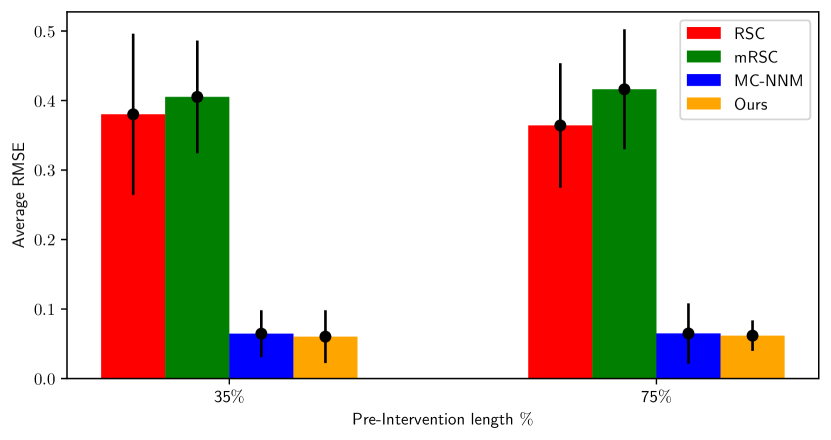
Figure 11: Average RMSE for post-intervention PreFF prediction across different pre-intervention lengths. Our method outperforms prior work on either pre-intervention lengths. Plotted at 90% confidence intervals.

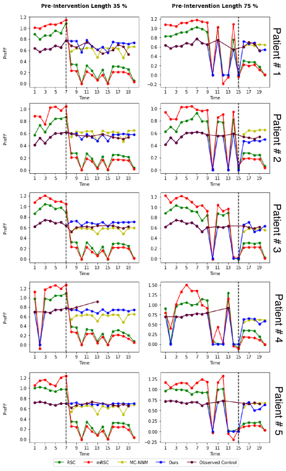
Figure 12: Estimates of PreFF for participants in the placebo group using other units in the placebo group as donors. The vertical black line indicates intervention instance. Our model reliably generates SC for both pre-intervention periods.

5.4 Me, My Doctor, and My Digital Twin: A Case Study on Friedreich’s Ataxia

FA is a fatal degenerative nervous system disorder with no cure. As a progressive disease with a wealth of available data and a growing number of potential therapeutic interventions, FA is one of the many genetic diseases that can benefit from precision medicine. We use clinical data collected during the FA Clinical Outcome Measure Study (FA-COMS) cohort [41], a natural history study involving yearly assessments of a core set of clinical measures and quality of life assessments, and maintained by the Critical Path Institute. 163 metrics were included in our model based on clinical relevance and minimal missing data. Each metric can be classified as 1) either longitudinal or static and 2) binary, ordinal, categorical, or continuous. Prior work only consider continuous data and unlike the generalized SCouT framework are therefore, not amenable to categorical data. A recent study found that Calcitriol, the active form of vitamin D, is able to increase Frataxin levels and restore mitochondrial function in cell models of FA. FA is caused by a deficiency of Frataxin, Accordingly, Calcitriol supplements could potentially improve health outcomes for FA patients [42]. We explore the effect of Calcitriol as an example of a synthetic medical intervention. Our resulting dataset tailored for the Calcitriol synthetic intervention analysis included $N=21$ donor units who indicated that they were taking a Calcitriol supplement at some point during the study and had sufficient pre-intervention data for training (see Appendix D.2 for data-formatting details). The dataset was aligned such that every donor patient began taking the supplement at $T_{0}=8$. A few patients never indicated that they had taken the supplement during the study period; hence, we set these patients as the target unit and simulated the counterfactual situation under which the patients do receive treatment at $T_{0}$. It is important to note that unlike randomized controlled trials, where we evaluate the effect of a treatment on the average individual, the synthetic intervention presents the predicted treatment effect on an individual patient, in line with the goals of precision medicine. Imagine a FA patient walking into a clinic, where the physician has access to data from patient’s previous health records and is deciding whether or not to recommend a Calcitriol supplement. The physician can use the synthetic intervention technique to generate a counterfactual under this treatment for any desirable metric, as we demonstrate next. We evaluated the patients on several rating scales commonly used for FA patients [43]:

• The FA Rating Scale neurologic examination (FARSn) [43] is one of the most used tests to evaluate an FA patient’s disease progression. It involves scoring on several subscales broadly divided into bulbar, lower limb, upper limb, peripheral nervous system and upright stability functionalities.

• The Nine-Hole Peg Test (9-HPT) is a quantitative measure of finger dexterity and is conducted on both the dominant and non-dominant arm, in that order. The patient is told to pick up and place pegs into open holes on a board in front of them.

• The Activities of Daily Living (ADL) Scale is widely used to rank adequacy and independence in basic tasks that a person could expect to encounter every day, including grooming, dressing, walking, and drinking.

We compare the predictions under the counterfactual scenario where the patients begin to take a Calcitriol supplement at time $T_{0}$ against the true observed values for the patients with no intervention. We included metrics from the FARSn, 9-HPT, and ADL exams that demonstrated the counterfactual under Calcitriol use for the patients. Fig. 13, Fig. 14, Fig.15 show the predictions for the FARSn, ADL, and 9-HPT scales, respectively. Most counterfactuals seem to suggest that Calcitriol use would have been beneficial with respect to all metrics highlighted below.

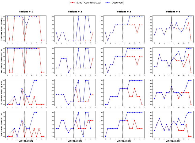
Figure 13: Tailored predictions for each patient under different FARSn scale metrics. The vertical black line indicates the intervention instance. A higher score is associated with a greater degree of disability. Except for patient 2, SCouT predicts considerable improvements after using Calcitriol.

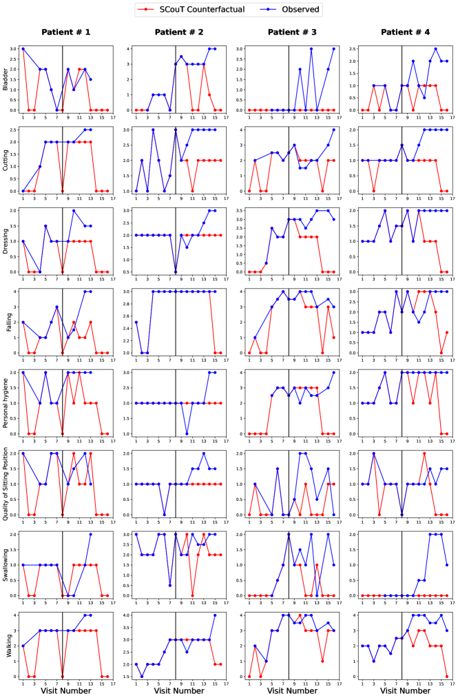
Figure 14: Tailored predicted scores for each patient under different ADL scale metrics. The vertical black line indicates intervention instance. A higher score is associated with a greater degree of disability. SCouT predicts considerable improvements after using Calcitriol across all metrics and all patients.

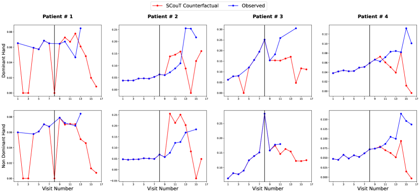
Figure 15: Tailored counterfactuals for each patient under 9-HPT metrics. The vertical black line indicates the intervention instance. The scores measure the time it takes for the patient to place the pegs into the hole; a higher score indicates a greater level of disability. SCouT predicts improvement in test times for all patients across both the dominant and non-dominant hands.

Across specific metrics and select patients, comparing the Calcitriol counterfactual and observed patient values also predicted little benefit from the supplement or were otherwise difficult to extract qualitative meaning from. Finally, none of the comparisons indicated that Calcitriol would allow further disease progression in the patients, which is comforting evidence that, at worst, Calcitriol has little effect. At best, the supplement could greatly improve the quality of life for a patient with FA.

6 Conclusion

SC-based methods paved the way for more effective techniques to estimate the counterfactual of a unit from several donor units. However, these methods are still restricted because they cannot capture inter-unit and intra-unit temporal contexts and are parametrically constrained to model linear dynamics. We introduced a Transformer-based Seq2Seq model that leverages local spatiotemporal relations to estimate the counterfactual sequence through multimodal inputs better and overcome these limitations. Experiments on synthetic and real-world data demonstrate that our model has high predictive power even in noisy data and donor pools of varying sizes. Explicitly modeling donor units is a strong inductive bias and significantly enhances predictive power compared to time series modeling. Our method leverages the Transformer model’s credit assignment ability to analyse the first-of-its-kind temporal evolution of donor contribution. We also demonstrated the applicability of our Transformer-based model in simulating counterfactual scenarios in healthcare, e.g., to accelerate in-silico clinical trials by simulating the control counterfactual for individuals in an Asthma randomized trial and generating the Calcitriol intervention counterfactual for FA patients. As big data and artificial intelligence continue to revolutionize healthcare, our work can be adapted for use beyond clinical trials and clinical decision-making and create measurable improvements in public health.

7 Acknowledgement

This work was supported by NSF Grant No. CCF-2203399. The experiments reported in this paper were performed on the computational resources managed and supported by Princeton Research Computing at Princeton University.

A Model Details

Our model is implemented using the Hugging Face library [44]. Our choice of the encoder-decoder model is a Bert2Bert model. The hyperparameters we use for various experiments are outlined in Table 2.

Table 2: Model and training hyperparameters

Hyperparameter	Value
Number of Layers	Synthetic: 3 Prop. 99: 3 Asthma: 4 FA: 4
Number of Attention Heads	1
Hidden Dimension	Synthetic: 32 Prop. 99: 128 Asthma: 128 FA: 128
Non linearity	GELU
Dropout	0.1
Pre-Intervention Length	Synthetic: 20 (N=5,10,15) 10 (N=25,50,75,100) Prop. 99: 5 Asthma: 2 FA: 5
Post-Intervention Length	Synthetic: 10 (N=5,10,15) 5 (N=25,50,75,100) Prop. 99: 2 Asthma: 2 FA: 2
#Singular Values Retained	Synthetic: 5 Prop. 99: 3 Asthma: 55 FA: 5
Learning Rate	$1\times 10^{-4}$
Weight Decay	$1\times 10^{-4}$
Warmup Steps (Pre-training)	Synthetic: $1\times 10^{4}$ Prop. 99: $1\times 10^{3}$ Asthma: $1\times 10^{4}$ FA: $1\times 10^{4}$
Pre-training Iterations	Synthetic: $5\times 10^{4}$ Prop. 99: $5\times 10^{3}$ Asthma: $5\times 10^{4}$ FA: $5\times 10^{4}$
Fine-tuning Iterations	Synthetic: $1\times 10^{4}$ Prop. 99: $1\times 10^{3}$ Asthma: $5\times 10^{3}$ FA: $5\times 10^{4}$
Batch Size	Synthetic: 128 Prop. 99: 64 Asthma: 16 FA: 16

B Proposition 99

Five covariates are used for generating the control:

• Per-capita cigarette consumption (in packs)

• Per-capita state personal income (logged)

• Per-capita beer consumption

• Percent of state population aged 15–24

• Average retail price per pack of cigarettes (in cents)

C Asthma

The CAMP dataset uses the Forced Expiratory Volume (FEV) and Forced Vital Capacity (FVC) as the lung functions. 16 continuous covariates from the dataset are used for generating the control:

• Pre-Bronchodilator FEV/FVC ratio % (PREFF)

• Age in years at randomization (age rz)

• Hemoglobin (hemog)

• Pre-Bronchodilator FEV (PREFEV)

• Pre-Bronchodilator FVC (PREFVC)

• Pre-Bronchodilator peak flow (PREPF)

• Post-Bronchodilator FEV (POSFEV)

• Post-Bronchodilator FVC (POSFVC)

• Post-Bronchodilator FEV/FVC ratio % (POSFF)

• Post-Bronchodilator peak flow (POSPF)

• Pre-Bronchodilator FEV % prediction (PREFEVPP)

• Pre-Bronchodilator FVC % prediction (PREFVCPP)

• Post-Bronchodilator FEV % prediction (POSFEVPP)

• Post-Bronchodilator FVC % prediction (POSFVCPP)

• White blood cell count (wbc)

• Age of current home (agehome)

D Friedreich’s Ataxia

D.1 FA Metrics

The following metrics were included in the clinical dataset for FA:

• Age of onset

• Length of shorter GAA Repeat

• Presence of point mutation

• Death Flag

• Ethnicity

• Sex

• Race

• Assistive Device Type

• Level of education

• Living circumstances

• The Friedreich ataxia Rating Scale neurologic (FARSn) examination subscores

• The Timed 25-Foot Walk

• The Nine-Hole Peg Test: Dominant Hand and Non-Dominant Hand

• Activities of Daily Living (ADL) Scale

• Bladder Control Scale

• Bowel Control Scale

• Impact of Visual Impairment Scale

• Modified Fatigue Impact Scale

• MOS Pain Effects Scale

• SF-10 and SF-36

D.2 Data Formatting for FA

Since the FA dataset we use comes from a natural history study that does not introduce any interventions itself, we have to reformat the dataset so it can be used for a synthetic intervention. The FA data includes longitudinal information regarding the medications a patient is taking. Out of all the patients, 72 indicated that they were taking a Calcitriol supplement at some point during the study. We manually searched for patients that reported taking Calcitriol for an extended period of time (typically 3 or more years) and had sufficient pre-intervention data for training. The resulting dataset tailored for the Calcitriol synthetic intervention analysis included $N=21$ and was aligned using the methodology from Figure 16. Thus every donor patient began taking the supplement at $T_{0}=8$. Four patients who had not taken the supplement during the study period, were then set as the target unit. Furthermore, the narrowed scope of the question we investigate in this section also gives us a use case to test our model on real world FA data with a much smaller number of donor units.

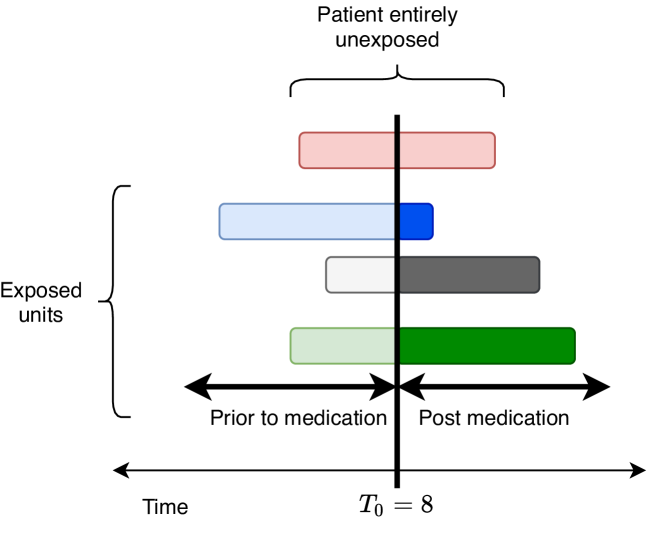
Figure 16: Dataset formatting to align all exposed units at a common intervention instance.

References

- [1] I. R. König, O. Fuchs, G. Hansen, E. von Mutius, and M. V. Kopp, “What is precision medicine?” European Respiratory Journal, vol. 50, no. 4, 2017.
- [2] B. Sibbald and M. Roland, “Understanding Controlled Trials: Why are Randomised Controlled Trials Important?” British Medical Journal, vol. 316, no. 7126, p. 201, 1998.
- [3] A. Abadie and J. Gardeazabal, “The economic costs of conflict: A case study of the Basque country,” American Economic Review, vol. 93, no. 1, pp. 113–132, Mar. 2003.
- [4] A. Abadie, A. Diamond, and J. Hainmueller, “Synthetic control methods for comparative case studies: Estimating the effect of California’s tobacco control program,” Journal of the American Statistical Association, vol. 105, no. 490, pp. 493–505, 2010.
- [5] C. Hsiao, H. S. Ching, and S. K. Wan, “A panel data approach for program evaluation: Measuring the benefits of political and economic integration of Hong Kong with Mainland China,” Journal of Applied Econometrics, vol. 27, no. 5, pp. 705–740, 2012.
- [6] N. Doudchenko and G. W. Imbens, “Balancing, regression, difference-in-differences and synthetic control methods: A synthesis,” CoRR, vol. abs/1610.07748, 2017.
- [7] M. Amjad, D. Shah, and D. Shen, “Robust synthetic control,” Journal of Machine Learning Research, vol. 19, no. 22, pp. 1–51, 2018.
- [8] M. Amjad, V. Misra, D. Shah, and D. Shen, “mRSC: Multi-dimensional robust synthetic control,” Proc. ACM Meas. Anal. Comput. Syst., vol. 3, no. 2, June 2019.
- [9] S. Athey, M. Bayati, N. Doudchenko, G. Imbens, and K. Khosravi, “Matrix completion methods for causal panel data models,” CoRR, vol. abs/1710.10251, 2017.
- [10] A. Agarwal, D. Shah, and D. Shen, “Synthetic interventions,” CoRR, vol. abs/2006.07691, 2020.
- [11] A. Vaswani, N. Shazeer, N. Parmar, J. Uszkoreit, L. Jones, A. N. Gomez, Ł. Kaiser, and I. Polosukhin, “Attention is all you need,” in Advances in Neural Information Processing Systems, vol. 30, 2017, pp. 5998–6008.
- [12] S. Cunningham and M. Shah, “Decriminalizing Indoor Prostitution: Implications for Sexual Violence and Public Health,” The Review of Economic Studies, vol. 85, no. 3, pp. 1683–1715, 2017.
- [13] S. Bohn, M. Lofstrom, and S. Raphael, “Did the 2007 legal Arizona Workers Act reduce the state’s unauthorized immigrant population?” The Review of Economics and Statistics, vol. 96, no. 2, pp. 258–269, 2014.
- [14] H. J. Kleven, C. Landais, and E. Saez, “Taxation and international migration of superstars: Evidence from the European football market,” American Economic Review, vol. 103, no. 5, pp. 1892–1924, 2013.
- [15] P. Pinotti, “The economic costs of organised crime: Evidence from Southern Italy,” The Economic Journal, vol. 125, no. 586, pp. F203–F232, 2015.
- [16] A. Abadie, “Using synthetic controls: Feasibility, data requirements, and methodological aspects,” Journal of Economic Literature, vol. 59, pp. 391–425, 2021.
- [17] Z. Qian, Y. Zhang, I. Bica, A. Wood, and M. van der Schaar, “Synctwin: Treatment effect estimation with longitudinal outcomes,” in Advances in Neural Information Processing Systems, vol. 34, 2021, pp. 3178–3190.
- [18] D. Card, “The impact of the Mariel boatlift on the Miami labor market,” ILR Review, vol. 43, no. 2, pp. 245–257, 1990.
- [19] D. Card and A. B. Krueger, “Minimum wages and employment: A case study of the fast food industry in New Jersey and Pennsylvania,” National Bureau of Economic Research, Working Paper 4509, Oct. 1993.
- [20] P. R. Rosenbaum and D. B. Rubin, “The Central Role of the Propensity Score in Observational Studies for Causal Effects,” Biometrika, vol. 70, no. 1, pp. 41–55, 1983.
- [21] G. W. Imbens and J. M. Wooldridge, “Recent developments in the econometrics of program evaluation,” Journal of Economic Literature, vol. 47, no. 1, pp. 5–86, Mar. 2009.
- [22] A. Abadie and M. D. Cattaneo, “Econometric methods for program evaluation,” Annual Review of Economics, vol. 10, no. 1, pp. 465–503, 2018.
- [23] C. Wing, K. Simon, and R. A. Bello-Gomez, “Designing difference in difference studies: Best practices for public health policy research,” Annual Review of Public Health, vol. 39, no. 1, pp. 453–469, 2018.
- [24] U. Shalit, F. D. Johansson, and D. Sontag, “Estimating individual treatment effect: Generalization bounds and algorithms,” CoRR, vol. abs/1607.03976, 2016.
- [25] J. Yoon, J. Jordon, and M. van der Schaar, “Ganite: Estimation of individualized treatment effects using generative adversarial nets,” in Proc. of the International Conference on Learning Representations, 2018.
- [26] I. Bica, A. M. Alaa, J. Jordon, and M. van der Schaar, “Estimating counterfactual treatment outcomes over time through adversarially balanced representations,” 2020.
- [27] X. Wang, D. Sontag, and F. Wang, “Unsupervised learning of disease progression models,” in Proc. of the 20th ACM SIGKDD International Conference on Knowledge Discovery and Data Mining, 2014, p. 85–94.
- [28] H. H. Nguyen, S. Saarakkala, M. B. Blaschko, and A. Tiulpin, “Climat: Clinically-inspired multi-agent transformers for knee osteoarthritis trajectory forecasting,” CoRR, vol. abs/2104.03642, 2021.
- [29] Y. Bengio, R. Ducharme, P. Vincent, and C. Janvin, “A neural probabilistic language model,” J. Mach. Learn. Res., vol. 3, no. null, p. 1137–1155, 2003.
- [30] T. Mikolov, M. Karafiát, L. Burget, J. H. Cernocký, and S. Khudanpur, “Recurrent Neural Network based Language Model,” in Proc. of the Conference of the International Speech Communication Association, 2010.
- [31] I. Sutskever, O. Vinyals, and Q. V. Le, “Sequence to sequence learning with neural networks,” CoRR, vol. abs/1409.3215, 2014.
- [32] A. Dosovitskiy, L. Beyer, A. Kolesnikov, D. Weissenborn, X. Zhai, T. Unterthiner, M. Dehghani, M. Minderer, G. Heigold, S. Gelly, J. Uszkoreit, and N. Houlsby, “An image is worth 16x16 words: Transformers for image recognition at scale,” in Proc. of the International Conference on Learning Representations, 2021.
- [33] J. Devlin et al., “BERT: Pre-training of deep bidirectional transformers for language understanding,” in Proc. of the Conference of the North American Chapter of the Association for Computational Linguistics: Human Language Technologies, vol. 1, 2019, pp. 4171–4186.
- [34] A. Radford, J. Wu, R. Child, D. Luan, D. Amodei, and I. Sutskever, “Language models are unsupervised multitask learners,” Technical Report, Open AI, 2019.
- [35] T. B. Brown, B. Mann, N. Ryder, M. Subbiah, J. Kaplan, P. Dhariwal, A. Neelakantan, P. Shyam, G. Sastry, A. Askell, S. Agarwal, A. Herbert-Voss, G. Krueger, T. Henighan, R. Child, A. Ramesh, D. M. Ziegler, J. Wu, C. Winter, C. Hesse, M. Chen, E. Sigler, M. Litwin, S. Gray, B. Chess, J. Clark, C. Berner, S. McCandlish, A. Radford, I. Sutskever, and D. Amodei, “Language models are few-shot learners,” CoRR, vol. abs/2005.14165, 2020.
- [36] K. He, X. Zhang, S. Ren, and J. Sun, “Deep residual learning for image recognition,” in Proc. of the IEEE Conference on Computer Vision and Pattern Recognition, June 2016.
- [37] J. L. Ba, J. R. Kiros, and G. E. Hinton, “Layer normalization,” CoRR, vol. abs/1607.06450, 2016.
- [38] C. D. Manning et al., “Emergent Linguistic Structure in Artificial Neural Networks Trained by Self-Supervision,” Proc. of the National Academy of Sciences, vol. 117, no. 48, pp. 30 046–30 054, 2020.
- [39] R. J. Williams and D. Zipser, “A learning algorithm for continually running fully recurrent neural networks,” Neural Computation, vol. 1, no. 2, pp. 270–280, 1989.
- [40] G. G. Shapiro et al., “The Childhood Asthma Management Program (CAMP): Design, Rationale, and Methods,” Controlled Clinical Trials, vol. 20, no. 1, pp. 91–120, Feb. 1999.
- [41] S. R. Regner et al., “Friedreich Ataxia Clinical Outcome Measures: Natural History Evaluation in 410 Participants,” J. Child Neurol., vol. 27, no. 9, pp. 1152–1158, Sep. 2012.
- [42] E. Britti, F. Delaspre, A. Sanz-Alcázar, M. Medina-Carbonero, M. Llovera, R. Purroy, S. Mincheva-Tasheva, J. Tamarit, and J. Ros, “Calcitriol Increases Frataxin Levels and Restores Mitochondrial Function in Cell Models of Friedreich ataxia,” Biochem. J., vol. 478, no. 1, pp. 1–20, 2021.
- [43] M. C. Fahey, L. Corben, V. Collins, A. J. Churchyard, and M. B. Delatycki, “How is Disease Progress in Friedreich’s Ataxia Best Measured? a Study of Four Rating Scales,” J. Neurol. Neurosurg. Psychiatry, vol. 78, no. 4, pp. 411–413, 2007.
- [44] T. Wolf et al., “Huggingface’s Transformers: State-of-the-art natural language processing,” CoRR, vol. abs/1910.03771, 2020.