Smart Multi-tenant Federated Learning

Abstract

Federated learning (FL) is an emerging distributed machine learning method that empowers in-situ model training on decentralized edge devices. However, multiple simultaneous training activities could overload resource-constrained devices. In this work, we propose a smart multi-tenant FL system, MuFL, to effectively coordinate and execute simultaneous training activities. We first formalize the problem of multi-tenant FL, define multi-tenant FL scenarios, and introduce a vanilla multi-tenant FL system that trains activities sequentially to form baselines. Then, we propose two approaches to optimize multi-tenant FL: 1) activity consolidation merges training activities into one activity with a multi-task architecture; 2) after training it for rounds, activity splitting divides it into groups by employing affinities among activities such that activities within a group have better synergy. Extensive experiments demonstrate that MuFL outperforms other methods while consuming 40% less energy. We hope this work will inspire the community to further study and optimize multi-tenant FL.

1 Introduction

Federated learning (FL) [40] has attracted considerable attention as it enables privacy-preserving distributed model training among decentralized devices. It is empowering growing numbers of applications in both academia and industry, such as Google Keyboard [18], medical imaging analysis [36, 49], and autonoumous vehicles [62, 45, 47]. Among them, some applications contain multiple training activities for different tasks. For example, Google Keyboard includes query suggestion [58], emoji prediction [48], and next-world prediction [18]; autonomous vehicles relates to multiple computer vision (CV) tasks, including object detection, tracking, and semantic segmentation [23].

However, multiple simultaneous training activities could overload edge devices [4]. Edge devices have tight resource constraints, whereas training deep neural networks for the aforementioned applications is resource-intensive. As a result, the majority of edge devices can only support one training activity at a time [37]; multiple simultaneous federated learning activities on the same device could overwhelm its memory, computation, and power capacities. Thus, it is important to navigate solutions to well coordinate these training activities.

A plethora of research on FL considers only one training activity in an application. Many studies are devoted to addressing challenges including statistical heterogeneity [35, 55, 56, 73, 60, 63], system heterogeneity [7, 57], communication efficiency [40, 30, 28, 67], and privacy issues [2, 22]. A common limitation is that they only focus on one training activity, but applications like Google Keyboard require multiple training activities for different targets [58, 18, 48]. Multi-tenancy of an FL system is designed in [4] to prevent simultaneous training activities from overloading devices. However, it mainly considers differences among training activities, neglecting potential synergies.

In this work, we propose a smart multi-tenant federated learning system, MuFL, to efficiently coordinate and execute simultaneous training activities under resource constraints by considering both synergies and differences among training activities. We first formalize the problem of multi-tenant FL and define four multi-tenant FL scenarios based on two variances in Section 3: 1) whether all training activities are the same type of application, e.g., CV applications; 2) whether all clients support all training activities. Then, we define a vanilla multi-tenant FL system that supports all scenarios by training activities sequentially. Built on it, we further optimize the scenario, where all training activities are the same type and all clients support all activities, by considering both synergies and differences among activities in Section 4. Specifically, we propose activity consolidation to merge training activities into one activity with a multi-task architecture that shares common layers and has specialized layers for each activity. We then introduce activity splitting to divide the activity into multiple activities based on their synergies and differences measured by affinities between activities.

We demonstrate that MuFL reduces the energy consumption by over 40% while achieving superior performance to other methods via extensive experiments on three different sets of training activities in Section 5. We believe that this work will inspire the community to further investigate and optimize multi-tenant FL. We summarize our contributions as follows:

• We formalize the problem of multi-tenant FL and define four multi-tenant FL scenarios. To the best of our knowledge, we are the first work that investigates multi-tenant FL in-depth.

• We propose MuFL, a smart multi-tenant federated learning system to efficiently coordinate and execute simultaneous training activities by proposing activity consolidation and activity splitting to consider both synergies and differences among training activities.

• We establish baselines for multi-tenant FL and demonstrate that MuFL elevates performance with significantly less energy consumption via extensive empirical studies.

2 Related Work

In this section, we first review the concept of multi-tenancy in cloud computing and machine learning. Then, we provide a literature review of multi-task learning and federated learning.

Multi-tenancy of Cloud Computing and Machine Learning   Multi-tenancy has been an important concept in cloud computing. It refers to the software architecture where a single instance of software serves multiple users [10, 15]. Multi-tenant software architecture is one of the foundations of software as a service (SaaS) applications [41, 31, 5]. Recently, researchers have adopted this idea to machine learning (especially deep learning) training and inference. Specifically, some studies investigate how to share GPU clusters to multiple users to train deep neural networks (DNN) [24, 65, 33], but these methods are for GPU clusters that have enormous computing resources, which are inapplicable to edge devices that have limited resources. Targeting on-device deep learning, some researchers define multi-tenant as processing multiple computer vision (CV) applications for multiple concurrent tasks [14, 25]. However, they focus on the multi-tenant on-device inference rather than training. On the contrary, we focus on multi-tenant federated learning (FL) training on devices, where the multi-tenancy refers to multiple concurrent FL training activities.

Multi-task Learning   Multi-task learning is a popular machine learning approach to learn models that generalize on multiple tasks [53, 64]. A plethora of studies investigate parameter sharing approaches that share common layers of a similar architecture [6, 13, 3, 44]. Besides, many studies employ new techniques to address the negative transfer problem [27, 66] among tasks, including soft parameter sharing [12, 43], neural architecture search [38, 21, 54, 17, 52], and dynamic loss reweighting strategies [29, 8, 59]. Instead of training all tasks together, task grouping trains only similar tasks together. The early works of task grouping [27, 32] are not adaptable to DNN. Recently, several studies analyze the task similarity [51] and task affinities [16] for task grouping. In this work, we adopt the idea of task grouping to consolidate and split training activities. The state-of-the-art task grouping methods [51, 16], however, are unsuitable for our scenario because they focus on the inference efficiency, bypassing the intensive computation on training. Thus, we propose activity consolidation and activity splitting to group training activities based on their synergies and differences.

Federated Learning   Federated learning emerges as a promising privacy-preserving distributed machine learning technique that uses a central server to coordinate multiple decentralized clients to train models [40, 26]. The majority of studies aim to address the challenges of FL, including statistical heterogeneity [35, 55, 56, 71, 63, 70, 72, 69], system heterogeneity [7, 57], communication efficiency [40, 30, 28, 67], and privacy concerns [2, 22]. Among them, federated multi-task learning [50, 39] is an emerging method to learn personalized models to tackle the statistical heterogeneity. However, these works mainly focus on training one activity in a client of an application. Multi-tenant FL that handles multiple concurrent training activities is rarely discussed [4]. In this work, we formalize the problem of multi-tenant FL, define four multi-tenant FL scenarios, and optimize one of the scenarios by considering both synergies and differences among training activities.

3 Problem Setup

This section provides preliminaries of federated learning (FL), presents the problem definition of multi-tenant FL, and classifies four multi-tenant FL scenarios. Besides, we introduce a vanilla multi-tenant FL system supports for all scenarios.

3.1 Preliminaries and Problem Definition

In the federated learning setting, the majority of studies consider optimizing the following problem:

$$\min_{\omega\in\mathbb{R}^{d}}f(\omega):=\sum_{k=1}^{K}p_{k}f_{k}(\omega):=\sum_{k=1}^{K}p_{k}\mathbb{E}_{\xi_{k}\sim\mathcal{D}_{k}}[f_{k}(\omega;\xi_{k})],$$ (1)

where $\omega$ is the optimization variable, $K$ is the number of selected clients to execute training, $f_{k}(\omega)$ is the loss function of client $k$, $p_{k}$ is the weight of client $k$ in model aggregation, and $\xi_{k}$ is the training data sampled from data distribution $\mathcal{D}_{k}$ of client $k$. FedAvg [40] is a popular federated learning algorithm, which sets $p_{k}$ to be proportional to the dataset size of client $k$.

Equation 1 illustrates the objective of single training activity in FL, but in real-world scenarios, multiple simultaneous training activities could overload edge devices. We further formalize the problem of multi-tenant FL as follows.

In multi-tenant FL, a server coordinates a set of clients $\mathcal{C}$ to execute a set of $n$ FL training activities $\mathcal{A}=\{\alpha_{1},\alpha_{2},\dots,\alpha_{n}\}$. It obtain a set of parameters of models $\mathcal{W}=\{\omega_{1},\omega_{2},\dots,\omega_{n}\}$, where each model $\omega_{i}$ is for activity $\alpha_{i}$. By defining $\mathcal{M}(\alpha_{i};\omega_{i})$ as performance measurement of each training activity $\alpha_{i}$, multi-tenant FL aims to maximize the performance of all training activities $\sum_{i=1}^{n}\mathcal{M}(\alpha_{i};\omega_{i})$, under the constraint that each client $k$ has limited memory budget and computation budget. These budgets constrain the number of concurrent training actvitities $n_{k}$ on client $k$. Besides, as devices have limited battery life, we would like to minimize the energy consumption and training time to obtain $\mathcal{W}$ from training activities $\mathcal{A}$.

3.2 Multi-tenant FL Scenarios

We classify multi-tenant FL into four different scenarios based on variances in two aspects: 1) whether all training activities in $\mathcal{A}$ are the same type of application, e.g., computer vision (CV) applications or natural language processing (NLP) applications; 2) whether all clients in $\mathcal{C}$ support all training activities in $\mathcal{A}$. We depict these four scenarios in Figure 6 in Appendix A and describe them below.

Scenario 1   $\forall\alpha_{i}\in\mathcal{A}$, $\alpha_{i}$ is the same type of application; $\forall\alpha_{i}\in\mathcal{A}$, $\forall c_{k}\in\mathcal{C}$ supports $\alpha_{i}$. For example, autonoumous vehicles (clients) support the same sets of CV applications, such as object detection and semantic segmentation. Thus, they support training activities of these applications.

Scenario 2   $\exists\alpha_{i}\in\mathcal{A}$, $\alpha_{i}$ is a different type of application; $\forall\alpha_{i}\in\mathcal{A}$, $\forall c_{k}\in\mathcal{C}$ supports $\alpha_{i}$. For example, Google Keyboard has different types of applications, including recommendation like query suggestion [58] and NLP like next-world prediction [18]. Smartphones (clients) installed Google Keyboard support these applications, thus, supporting all related training activities.

Scenario 3   $\forall\alpha_{i}\in\mathcal{A}$, $\alpha_{i}$ is the same type of application; $\forall\alpha_{i}\in\mathcal{A}$, $\exists c_{k}\in\mathcal{C}$ does not support $\alpha_{i}$. For example, survelliance cameras (clients) in parking lots could support CV applications, but cameras in different locations may support different applications, e.g., counting open-parking spots, tracking parking duration, or recording fender benders.

Scenario 4   $\exists\alpha_{i}\in\mathcal{A}$, $\alpha_{i}$ is a different type of application; $\forall\alpha_{i}\in\mathcal{A}$, $\exists c_{k}\in\mathcal{C}$ does not support $\alpha_{i}$. For example, browsers (clients) could leverage users’ browsing history to support browsing history suggestion [19] and recommendations [42], which are different types of applications. Some users may opt-out the recommendations, resulting in not all browsers need to support all training activities.

The application determines the multi-tenant FL scenario. We next introduce a vanilla multi-tenant FL that supports all these scenarios as our baseline.

3.3 Vanilla Multi-tenant FL

Figure 1(a) presents the architecture of a vanilla multi-tenant FL system. It prevents overloading and congestion of multiple simultaneous training activities by scheduling them to execute one by one. Particularly, we design a scheduler to queue training activities in the server. In each round, the server selects $K$ clients from the client pool to participate in training. Depending on the computational resources of the selected clients, the server can execute training for multiple activities concurrently if the clients have enough computation resources. In this study, we assume that each client can execute one training activity at a time ($n_{k}$ = 1). This is a realistic assumption for the majority of current edge devices. As a result, the vanilla multi-tenant FL system executes training activities sequentially.

The vanilla multi-tenant FL system supports the four multi-tenant FL scenarios discussed above. From the perspective of the type of application, it can handle different application types of training activities as each training activity is executed independently. From the perspective of whether clients support all training activities, each training activity can select clients that support the activity to participate in training. Despite its comprehensiveness, it only considers differences among training activities, neglecting their potential synergies. In contrast, our proposed MuFL considers both synergies and differences among training activities to further optimize the Scenario 1. MuFL can be view as a generalization of the vanilla multi-tenant FL system; it can be specialized to the vanilla multi-tennat FL system by disabling activity consolidation and activity splitting. It is also adaptable to Scenario 3 and 4 by employing strategies to filter out clients that do not support all training activities, but we keep them for future investigation.

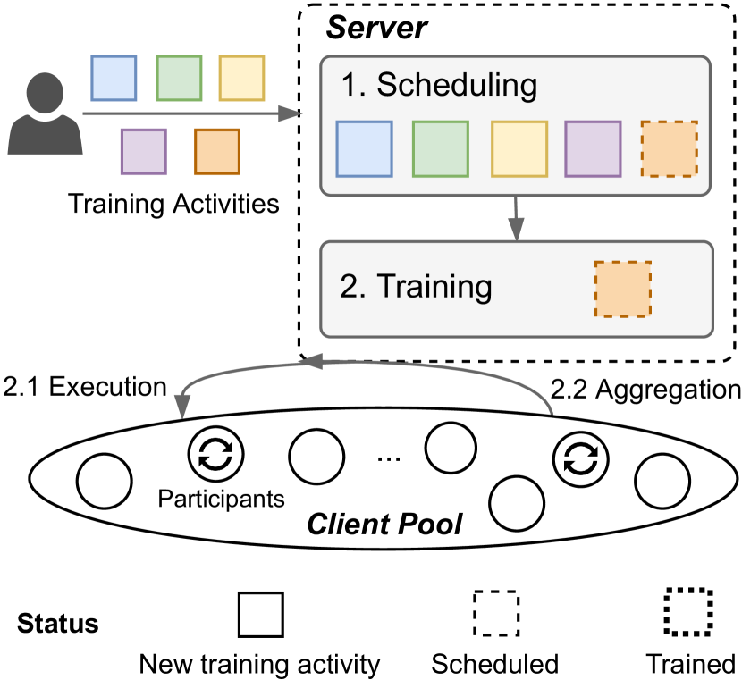
(a) Vanilla Multi-tenant FL

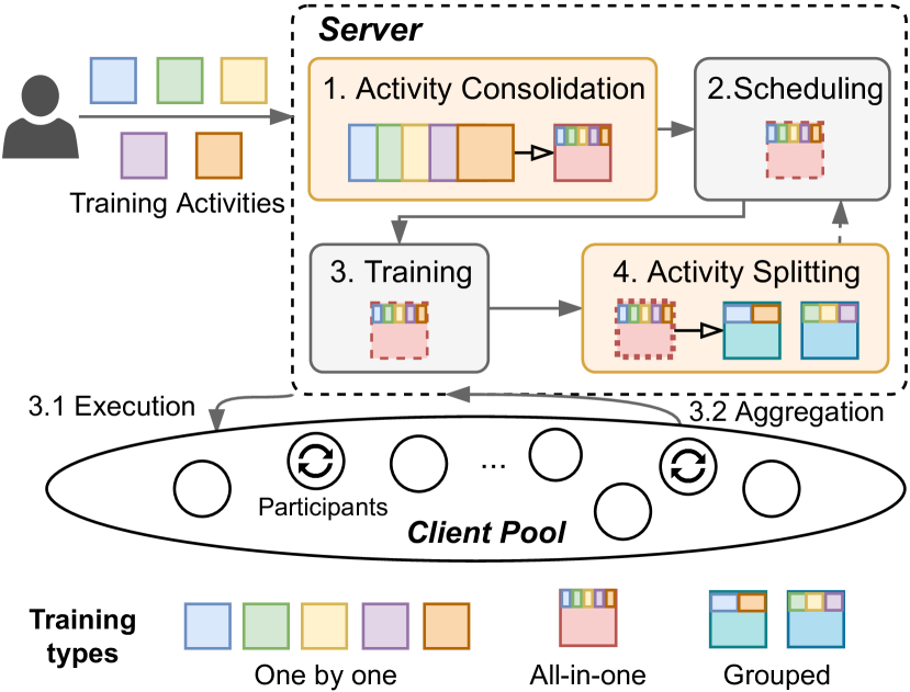
(b) Smart Multi-tenant FL

Figure 1: The architectures of proposed multi-tenant federated learning (FL) systems. The vanilla multi-tenant FL system (a) employs a scheduler to queue simultaneous training activities and execute them one by one. The smart multi-tenant FL system (b) proposes activity consolidation and activity splitting to consider both synergies and differences among training activities, which elevates performance and reduces resource consumption.

4 Smart Multi-tenant FL

In this section, we introduce the smart multi-tenant FL system, MuFL. We start by providing an overview of MuFL. Then, we present two important components of MuFL, activity consolidation and activity splitting, to consider both synergies and differences among simultaneous training activities.

Figure 1(b) depicts the architecture and training processes of MuFL. It contains a server to coordinate training activities and a pool of clients to execute training. MuFL optimizes the Scenario 1 discussed previously with the following steps: 1) The server receives training activities $\mathcal{A}=\{\alpha_{1},\alpha_{2},\dots,\alpha_{n}\}$ to train models $\mathcal{W}=\{\omega_{1},\omega_{2},\dots,\omega_{n}\}$ and consolidates these activities into an all-in-one training activity $\alpha_{0}$; 2) The server schedules $\alpha_{0}$ to train; 3) The server select $K$ clients from the client pool to execute $\alpha_{0}$ iteratively through FL process for $R_{0}$ rounds; 4) The server splits the all-in-one activity $\alpha_{0}$ into multiple training activity groups $\{\mathcal{A}_{1},\mathcal{A}_{2},\dots\}$, where each group trains nonoverlapping subset of $\mathcal{W}$. 5) The server iterates step 2 and 3 to train $\mathcal{A}_{j}$. We summarize MuFL in Algorithm 1 in Appendix D and introduce the details of activity consolidation and activity splitting next.

4.1 Activity Consolidation

Focusing on optimizing the Scenario 1 of multi-tenant FL, we first propose activity consolidation to consolidate multiple training activities into an all-in-one training activity, as illustrated in the first step of Figure 1(b). In Scenario 1, all training activities are the same type of application and all clients support all training activities. Since training activities $\mathcal{A}=\{\alpha_{1},\alpha_{2},\dots,\alpha_{n}\}$ are of the same type, e.g., CV or NLP, models $\mathcal{W}=\{\omega_{1},\omega_{2},\dots,\omega_{n}\}$ could share the same backbone (common layers). Thus, we can consolidate $\mathcal{A}$ into an all-in-one training activity $\alpha_{0}$ that trains a multi-task model $\nu=\{\theta_{s}\}\cup\{\theta_{\alpha_{i}}|\alpha_{i}\in\mathcal{A}\}$, where $\theta_{s}$ is the shared model parameters and $\theta_{\alpha_{i}}$ is the specific parameters for training activity $\alpha_{i}\in\mathcal{A}$.

Activity consolidation leverages synergies among training activities and effectively reduces the computation cost of multi-tenant FL from multiple trainings into a single training. However, simply employing activity consolidation is another extreme of multi-tenant FL that only considers synergies among activities. As shown in Figure 2, all-in-one method is efficient in energy consumption, but it leads to unsatisfactory performance. Consequently, we further propose activity splitting to consider both synergies and differences among training activities.

4.2 Activity Splitting

We propose activity splitting to divide the all-in-one activity $\alpha_{0}$ into multiple groups after it is trained for certain rounds. Essentially, we aim to split $\mathcal{A}=\{\alpha_{1},\alpha_{2},\dots,\alpha_{n}\}$ into multiple nonoverlapping groups such that training activities within a group have better synergy. Let $\{\mathcal{A}_{1},\mathcal{A}_{2},\dots,\mathcal{A}_{m}\}$ be subsets of $\mathcal{A}$, we aim to find a set $I\subseteq\{1,2,\dots,m\}$ such that $|I|\leq|\mathcal{A}|$, $\bigcup_{j\in I}\mathcal{A}_{j}=\mathcal{A}$, and $\bigcap_{j\in I}\mathcal{A}_{j}=\emptyset$. Each group $\mathcal{A}_{j}$ trains a model $\nu_{j}=\{\theta_{s}^{j}\}\cup\{\theta_{\alpha_{i}}|\alpha_{i}\in\mathcal{A}_{j}\}$, which is a multi-task network when $\mathcal{A}_{j}$ contains more than one training activity, where $\theta_{s}^{j}$ is the shared model parameters and $\theta_{\alpha_{i}}$ is the specific parameters for training activity $\alpha_{i}\in\mathcal{A}_{j}$. The core question is how to determine set $I$ to split these activities considering their synergies and differences.

Inspired by TAG [16] that measures task affinites for task grouping, we employ affinities between training activities for activity splitting via three stages: 1) we measure affinities among activities during all-in-one training; 2) we select the best combination of splitted training activities based on affinity scores; 3) we continue training each split with its model initialized with parameters obtained from all-in-one training. Particularly, during training of all-in-one activity $\alpha_{0}$, we measure the affinity of training activity $\alpha_{i}$ onto $\alpha_{j}$ at time step $t$ in each client $k$ with the following equation:

$$\mathcal{S}^{k,t}_{\alpha_{i}\rightarrow\alpha_{j}}=1-\frac{\mathcal{L}_{\alpha_{j}}(\mathcal{X}^{k,t},\theta_{s,\alpha_{i}}^{k,t+1},\theta_{\alpha_{j}}^{k,t})}{\mathcal{L}_{\alpha_{j}}(\mathcal{X}^{k,t},\theta_{s}^{k,t},\theta_{\alpha_{j}}^{k,t})},$$ (2)

where $\mathcal{L}_{\alpha_{j}}$ is the loss function of $\alpha_{j}$, $\mathcal{X}^{k,t}$ is a batch of training data, and $\theta_{s}^{k,t}$ and $\theta^{k,t+1}_{s,\alpha_{i}}$ are the shared model parameters before and after updated by $\alpha_{i}$, respectively. Positive value of $\mathcal{S}^{k,t}_{\alpha_{i}\rightarrow\alpha_{j}}$ means that activity $\alpha_{i}$ helps reduce the loss of $\alpha_{j}$. This equation measures the affinity of one time-step of one client. We approximate affinity scores for each round by averaging the values over $T$ time-steps in $E$ local epochs and $K$ selected clients: $\hat{\mathcal{S}}_{\alpha_{i}\rightarrow\alpha_{j}}=\frac{1}{KET}\sum_{k=1}^{K}\sum_{e=1}^{E}\sum_{t=1}^{T}\mathcal{S}^{k,t}_{\alpha_{i}\rightarrow\alpha_{j}}$, where $T$ is total time steps determined by the frequency $f$ of calculating Equation 2, e.g., $f=5$ means measuring the affinity in each client in every five batches.

These affinity scores measure pair-wise affinities between traininig activities. We next use them to calculate total affinity scores of a grouping with $\sum_{i=1}^{n}\hat{\mathcal{S}}_{\alpha_{i}}$, where $\hat{\mathcal{S}}_{\alpha_{i}}$ is the averaged affinity score onto each training activity. For example, in a grouping of two splits of five training activities $\{\{\alpha_{1},\alpha_{2}\},\{\alpha_{3},\alpha_{4},\alpha_{5}\}\}$, where $\{\alpha_{1},\alpha_{2}\}$ is one split and $\{\alpha_{3},\alpha_{4},\alpha_{5}\}$ is another split. The affinity score onto $\alpha_{1}$ is $\hat{\mathcal{S}}_{\alpha_{1}}=\hat{\mathcal{S}}_{\alpha_{2}\rightarrow\alpha_{1}}$ and the affinity score onto $\alpha_{3}$ is ${\hat{\mathcal{S}}_{\alpha_{3}}}=(\hat{\mathcal{S}}_{\alpha_{4}\rightarrow\alpha_{3}}+\hat{\mathcal{S}}_{\alpha_{5}\rightarrow\alpha_{3}})/2$. Consequently, we can find the set $I$ with $|I|$ elements for subsets of $\mathcal{A}$ that maximize $\sum_{i=1}^{n}\hat{\mathcal{S}}_{\alpha_{i}}$, where $|I|$ defines the number of elements. Although this problem is a NP-hard problem (similar to Set-Cover problem), we can solve it with algorithms like branch-and-bound methods [51, 34].

We would like to further highlight the differences between our method and TAG [16]. Firstly, TAG allows overlapping task grouping that could train one task multiple times because it focuses on inference efficiency. In contrast, our focus is fundamentally different; we focus on training efficiency and thus our method considers only nonoverlapping activity splitting. Secondly, TAG is computation-intensive to compute higher numbers of splits, e.g., it fails to produce results of five splits in a week, whereas we only need seconds of computation. Thirdly, TAG sets $\hat{\mathcal{S}}_{\alpha_{i}\rightarrow\alpha_{i}}=1e^{-6}$ in implementation, which rules out the possibility that a group only contains one task as it results in much smaller value than other groupings. Besides, $\hat{\mathcal{S}}_{\alpha_{i}\rightarrow\alpha_{i}}$ calculated from Equation 2 is also not desirable because it is much larger (could be 10x larger) than other affinity scores, resulting in a group that always contains one task. To overcome these issues, we propose a new method to calculate this value:

$$\hat{\mathcal{S}}_{\alpha_{i}\rightarrow\alpha_{i}}=\sum_{j\in\mathcal{N}\backslash\{i\}}\frac{(\hat{\mathcal{S}}_{\alpha_{i}\rightarrow\alpha_{j}}+\hat{\mathcal{S}}_{\alpha_{j}\rightarrow\alpha_{i}})}{2n-2},$$ (3)

where $\mathcal{N}=\{1,2,\dots,n\}$. The intuition is that it measures the normalized affinity of activity $\alpha_{i}$ to other activities and other activities to $\alpha_{i}$. Fourthly, we focus on the multi-tenant FL scenario, thus, we propose to aggregate the affinity scores over $K$ selected clients. Fifthly, TAG trains each set $\mathcal{A}_{j}$ from scratch, whereas we train each set $\mathcal{A}_{j}$ by initializing models with the parameters obtained from $R_{0}$ rounds of all-in-one training.

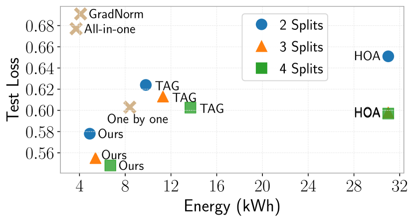
(a) A set of five training activities: sdnkt

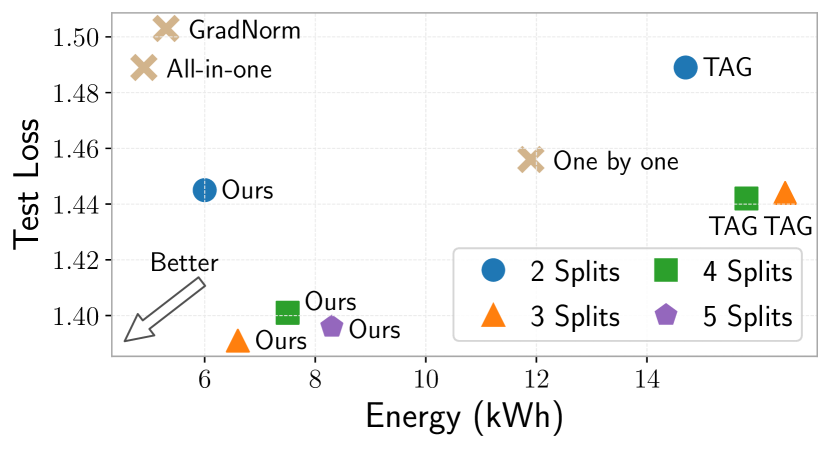
(b) A set of nine trianing activities: sdnkterca

Figure 2: Comparison of test loss and energy consumption on two training activity sets: (a) sdnkt and (b) sdnkterca, where each character represents an activity. Compared with all-in-one methods, our method achieves much better performance with slight increases in computation. Moreover, our method achieves the best performance while consuming less energy than the other methods.

5 Experiments

We evaluate the performance and resource usage of MuFL and design our experiments to answer the following questions: 1) How effective is our activity splitting approach? 2) When to split the training activities? 3) Is it beneficial to iteratively split the training activities? 4) What is the impact of local epoch and scaling up the number of selected clients in each training round?

Experiment Setup

We construct the Scenario 1 of multi-tenant FL scenarios using Taskonomy dataset [61], which is a large computer vision dataset of indoor scenes of buildings. We run experiments with $N=32$ clients, where each client contains a dataset of a building to simulate the statistical heterogeneity in FL. Three sets of training activities are used to evaluate the robustness of MuFL: sdnkt, erckt, and sdnkterca; each character represents an activity, e.g., s and d represents semantic segmentation and depth estimation, respectively. We measure the statistical performance of an activity set using the sum of test losses of individual activities. By default, we use $K=4$ selected clients and $E=1$ local epoch. More experimental details are provided in Appendix B.

5.1 Performance Evaluation

We compare the performance, in terms of test loss and energy consumption, among the following methods: 1) one by one training of activities (i.e., the vanilla multi-tenant FL); 2) all-in-one training of activities (i.e., using only activity consolidation); 3) all-in-one training with gradient normalization applied to tune the gradient magnitudes among activities (GradNorm [8]); 4) estimating higher-order of activity groupings from pair-wise activities performance (HOA [51]); 5) grouping training activities with only task affinity grouping method (TAG [16]); 6) MuFL with both activity consolidation and activity splitting. Carbontracker [1] is used to measure energy consumption and carbon footprint (provided in Appendix C). We report results of multiple splits in activity splitting.

Figure 2 compares performance of the above methods on activity sets sdnkt and sdnkterca. The methods that achieve lower test loss and lower energy consumption are better. At the one extreme, all-in-one methods (including GradNorm) consume the least energy, but their test losses are the highest. At the other extreme, HOA [51] achieves comparable test losses on three or four splits of sdnkt, but it demands high energy consumption ($\sim 4-6\times$ of ours) to compute pair-wise activities for higher-order estimation. Although training activities one by one and TAG [16] present a good balance between test loss and energy consumption, MuFL is superior in both aspects; it achieves the best test loss with $\sim$40% and $\sim$50% less energy consumption on activity set sdnkt and sdnkterca, respectively. Additionally, more splits of activity in the activity splitting lead to higher energy consumption, but it could help further reduce test losses. We do not report HOA [51] for activity set sdnkterca due to computation constraints as it requires computing at least 36 pair-wise training activities ($\sim$720 GPU hours); its energy consumption is estimated to be $\sim 12\times$ of ours. We provide test losses of each activity, the results of splits, and results of activity set erckt in Appendix C.

5.2 How Effective is Our Activity Splitting Approach?

Table 1: Performance (test loss) comparison of our method with the optimal and worst splits. Our method achieves the best performance, indicating the effectiveness of our activity splitting method.

Activity	Splits	Ours	Train from Sctrach			Train from Initialization
Set			Optimal	Worst		Optimal	Worst
sdnkt	2	0.578 ± 0.015	0.622 ± 0.007	0.685 ± 0.010		0.595 ± 0.008	0.595 ± 0.004
	3	0.555 ± 0.008	0.585 ± 0.026	0.674 ± 0.022		0.560 ± 0.006	0.578 ± 0.006
erckt	2	1.039 ± 0.024	1.070 ± 0.013	1.312 ± 0.065		1.048 ± 0.024	1.068 ± 0.037
	3	1.015 ± 0.018	1.058 ± 0.029	1.243 ± 0.099		1.020 ± 0.012	1.052 ± 0.026

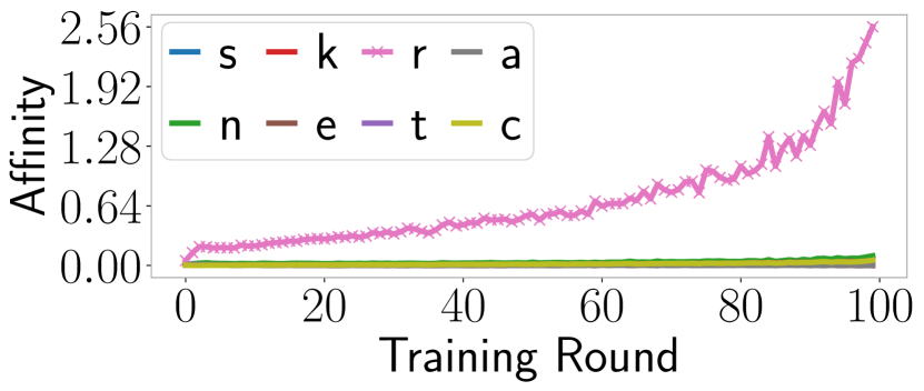
(a) Affinities to activity d

(b) Affinities to activity r

(c) Affinities to activity s

Figure 3: Changes of affinity scores of one activity to the other over the course of training on activity set sdnkterca. Activities d and r have high inter-activity affinity scores. The trends of affinities emerge at the early stage of training.

We demonstrate the effectiveness of our activity splitting approach by comparing it with the possible optimal and worst splits. The optimal and worst splits are obtained with two steps: 1) we measure the performance over all combinations of two splits and three splits of an activity set by training them from scratch; 2) we select the combination that yields the best performance as the optimal split and the worst performance as the worst split.

Table 1 compares the test loss of MuFL with the optimal and worst splits trained in two ways: 1) training each split from scratch; 2) training each split the same way as our activity splitting — initializing models with the parameters obtained from all-in-one training. On the one hand, training from initialization outperforms training from scratch in all settings. It suggests that initializing each split with all-in-one training model parameters can significantly improve the performance. On the other hand, our activity splitting method achieves the best performance in all settings, even though training from initialization reduces the gaps of different splits (the optimal and worst splits). These results indicate the effectiveness of our activity splitting approach.

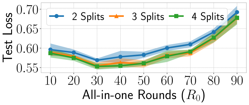
(a) Training activity set: sdnkt

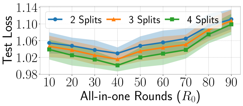
(b) Training activity set: erckt

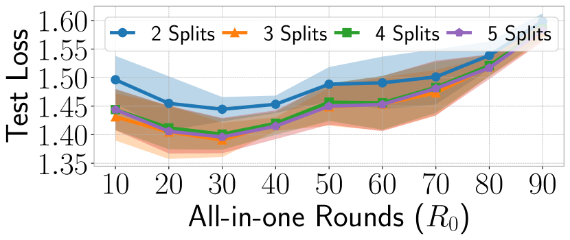
(c) Training activity set: sdnkterca

Figure 4: Performance comparison of training all-in-one activities for different $R_{0}$ rounds. Fixing the total training rounds $R=100$, our method achieves the best performance when $R_{0}=\{20,30,40\}$ rounds, varied over activity sets.

Table 2: Performance of hierarchical splitting on three activity sets sdnkt, erckt, and sdnkterca. Hierarchical splitting outperforms two splits and achieves similar performance to three splits with less energy (kWh) consumption.

Method	sdnkt			erckt			sdnkterca
	Energy	Test Loss		Energy	Test Loss		Energy	Test Loss
Two Splits	4.9 ± 0.3	0.578 ± 0.015		6.7 ± 0.2	1.039 ± 0.024		6.0 ± 0.1	1.445 ± 0.021
Three Splits	5.4 ± 0.7	0.555 ± 0.008		7.2 ± 0.2	1.015 ± 0.018		6.6 ± 0.4	1.391 ± 0.030
Hierarchical	5.3 ± 0.4	0.563 ± 0.007		6.9 ± 0.2	1.022 ± 0.020		6.5 ± 0.3	1.403 ± 0.024

5.3 When to Split Training Activities?

We further answer the question that how many $R_{0}$ rounds should we train the all-in-one activity before activity splitting. It is determined by two factors: 1) the rounds needed to obtain affinity scores for a reasonable activity splitting; 2) the rounds that yield the best overall performance.

Affinity Analysis   We analyze changes in affinity scores over the course of training to show that early-stage affinity scores are acceptable for activity splitting. Figure 3 presents the affinity scores of different activities to one activity on activity set sdnkterca. Figure 3(a) and 3(b) indicate that activity d and activity r have high inter-activity affinity scores; they are divided into the same group as a result. In contrast, both d and r have high affinity score to activity s in Figure 3(c), but not vice versa. These trends emerge in the early stage of training, thus, we employ the affinity scores of the tenth round for activity splitting for the majority of experiments; they are effective in achieving promising results as shown in Figure 2 and Table 1. We provide more affinity scores of other activities in Appendix C.

The Impact of $R_{0}$ Rounds   Figure 4 compares the performance of training $R_{0}$ for 10 to 90 rounds before activity splitting on three activity sets. Fixing the total training round $R=100$, we train each split of activities for $R_{1}=R-R_{0}$ rounds. The results indicate that MuFL achieves the best performance when $R_{0}=\{20,30,40\}$ rounds, varied over activity sets. Training the all-in-one activity for enough rounds helps utilize benefits and synergies of training together, but training for too many rounds almost suppresses the benefits of considering differences among activities. We suggest training $R_{0}$ for [20, 40] that strikes a good balance between these two extremes.

5.4 Hierarchical Splitting

This section evaluates an alternative adaptive hierarchical activity splitting strategy. In activity splitting, we can divide the all-in-one training activity into $\{2,3,\dots\}$ splits. As shown in Figure 2, more splits lead to better performance with slightly higher energy consumption in the five-activity set, but the trend is not straightforward in the nine-activity set. Apart from setting the number of splits directly, MuFL can split the training activity into more splits adaptively via two steps: 1) dividing the all-in-one activity into two splits and training each one for $R_{1}$ rounds; 2) further dividing one of them to two splits and train these three activities for $R_{2}$ rounds. We term it as hierarchical splitting that adaptively divides activities into more splits.

Table 2 compares the performance of hierarchical splitting (3 splits) with directly splitting to multiple splits on three activity sets sdnkt, erckt, and sdnkterca. We use $R_{0}=30$, $R_{1}=40$, and $R_{2}=30$ for sdnkt and erckt, and $R_{0}=30$, $R_{1}=20$, and $R_{2}=50$ for sdnkterca. Hierarchical splitting effectively reduces test losses of two splits and achieves comparable performance to three splits with less energy consumption. These results suggest that hierarchical splitting can be an alternative method of activity splitting, which could be useful without determining the number of splits beforehand. Additionally, these results also demonstrate the possibility of other activity splitting strategies to be considered in future works.

5.5 Additional Ablation Studies

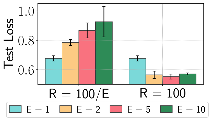
(a) Impact of $E$

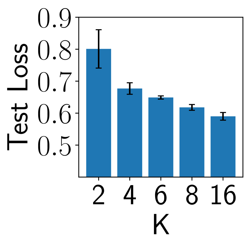
(b) Impact of $K$

Figure 5: Ablation studies on the impact of FL settings on activity set sdnkt: (a) local epoch $E$; (b) the number of selected clients $K$. Larger $E$ (with $R=100$) and $K$ requires higher computation. They could reduce losses, but the marginal benefit decreases as computation increases.

This section provides ablation studies of the impact of local epoch $E$ and the number of selected clients $K$ in FL using all-in-one training. We report the results of activity set sdnkt here and provide more results in Appendix C.

Impact of Local Epoch $E$   Local epoch defines the number of epochs each client trains before uploading training updates to the server. The total computation is $R*E$, where $R$ is the total training rounds. Figure  5(a) compares test losses of local epochs $E=\{1,2,5,10\}$. On the one hand, fixing the total computation ($R=\nicefrac{{100}}{{E}}$), larger $E$ results in performance degradation. One the other hand, fixing training rounds $R=100$, larger $E$ could lead to better performance, which is especially effective when $E$ increases from $E=1$ to $E=2$. However, such improvement is not consistant when $E=10$. It suggests the limitation of simply increasing computation with larger $E$ in improving performance. Note that MuFL (Table 1) achieves better results than $E=5$ with $\sim 5\times$ less computation.

Impact of The Number of Selected Clients $K$   Figure 5(b) compares test losses of the number of selected clients $K=\{2,4,6,8,16\}$ in each round. Increasing the number of selected clients improves the performance, but the effect becomes marginal as $K$ increases. Larger $K$ can also be considered as using more computation in each round. Similar to the results of the impact of $E$, simply increasing computation can only improve performance to a certain extent. It also shows the significance of MuFL that increases performance with slightly more computation. We use $K=4$ by default for experiments and demonstrate that MuFL is also effective on $K=8$ in Appendix C.

6 Conclusions and Discussions

In this work, we propose a smart multi-tenant federated learning system to effectively coordinate and execute multiple simultaneous FL training activities. In particular, we introduce activity consolidation and activity splitting to consider both synergies and differences among training activities. Extensive empirical studies demonstrate that our method is effective in elevating performance and significant in reducing energy consumption and carbon footprint by more than 40%, which are important metrics to our society. We believe that multi-tenant FL will emerge and empower many real-world applications with the fast development of FL. We hope this research will inspire the community to further work on algorithm and system optimizations of multi-tenant FL. Future work involves designing better scheduling mechanisms to coordinate training activities, employing and integrating client selection strategies to optimize resource and training allocation, and extending our optimization approaches to other multi-tenant FL scenarios. Lastly, studies of FL are closely related to data privacy risks and the fairness among training activities could also be considered; the applications of multi-tenant FL should seek tools and new approaches to address these issues.

The following appendixes provide supplemental material for the main manuscript. We update two parts compared to the one appended at the end of the main paper: 1) we update three runs of experiment results in Figure 13(a) and Figure 13(b); 2) we provide results of standalone training that conducts training using data in each client independently in Figure 14.

Appendix A Multi-tenant FL Scenarios

We introduce four multi-tenant federated learning scenarios in Section 3. Figure 6 depicts these four scenarios with variances in two aspects: 1) whether all training activities are the same type of application, e.g., CV applications; 2) whether all clients support all training activities.

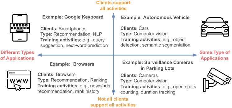
Figure 6: Illustration of the four multi-tenant FL scenarios.

Appendix B Experimental Details

This section provides more experimental information, including dataset, implementation details, and computation resources used.

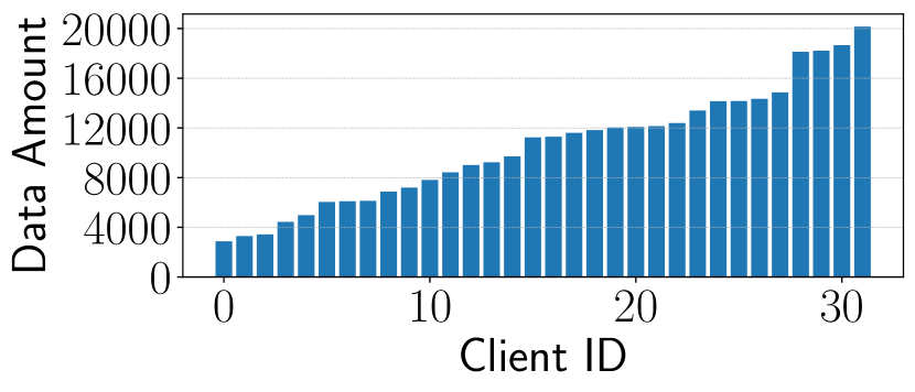
Figure 7: The data amount distribution of each training activity over 32 clients.

Dataset

We run experiments using Taskonomy dataset [61], which is a large computer vision (CV) dataset of indoor scenes of buildings. To facilitate reproducibility and mitigate computational requirements, we use the tiny split of Taskonomy dataset, whose size is around 445GB. We select nine CV applications to form three sets of training activities: sdnkt, erckt, sdnkterca. These nine actvities are also used in [51]. Figure 8 provides sample images of these nine training activities, as well as the representation of each character. In particular, we employ indoor images of 32 buildings as the total number of clients $N=32$; each client contains images of a building to simulate the statistical heterogeneity. On the one hand, clients have different sizes of data. Figure 7 shows the distribution of dataset sizes of an activity of clients. On the other hand, Figure 9 shows sample images of five clients; their indoor scenes vary in design, layout, objects, and illumination.

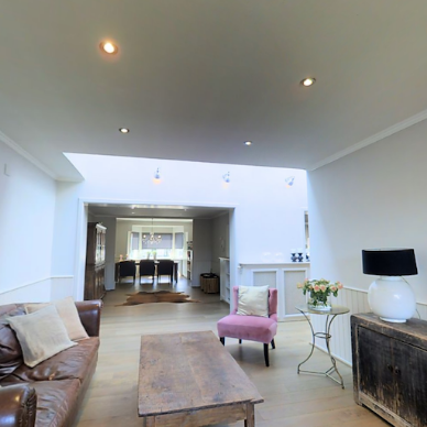
(a) Input Image

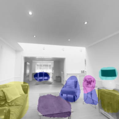
(b) s: Segmentation

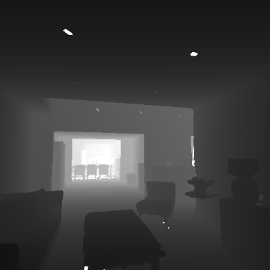
(c) d: Depth Estimation

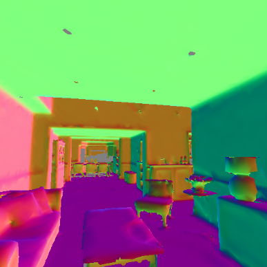
(d) n: Normal

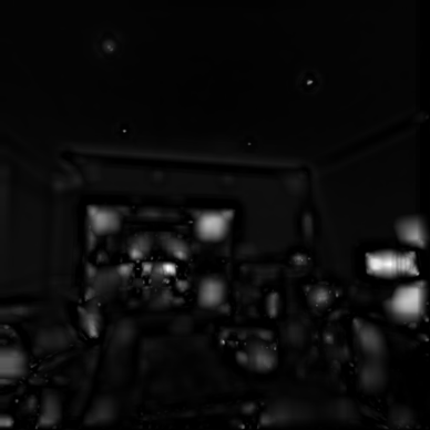
(e) k: Keypoint

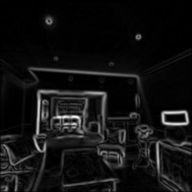
(f) t: Edge Texture

(g) e: Edge Occlusion

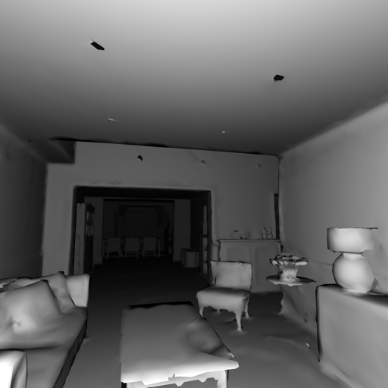
(h) r: Reshasing

(i) c: Principle Curvature

(j) a: Auto-encoder

Figure 8: Sample images of nine training activities corresponding to the input image.

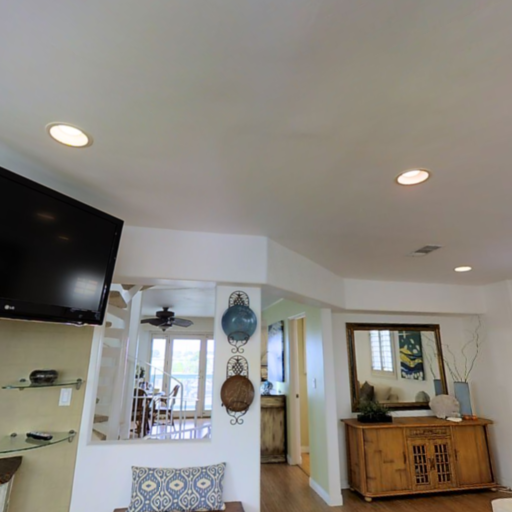
Figure 9: Sample images of five clients, where each client contains indoor scenes of a building. These indoor images differ in design, layout, objects, and illumination.

Implementation Details

We implement multi-tenant FL systems in Python using EasyFL [68] and PyTorch [46]. We simulate the FL training on a cluster of NVIDIA Tesla V100 GPUs, where each node in the cluster contains 8 GPUs. In each round, each selected client is allocated to a GPU to conduct training; these clients communicate via the NCCL backend. Besides, we employ FedAvg [40] for the server aggregation. By default, we randomly select $K=4$ clients to train for $E=1$ local epochs in each round and train for $R=100$ rounds.

We reference the implementation of multi-task learning from [51]’s official repository for all-in-one training and training of each split after activity splitting. Particularly, the network architecture contains an encoder $\theta_{s}$ and multiple decoders $\theta_{\alpha_{i}}$; one decoder for a training activity $\alpha_{i}$. We use the modified Xception Network [9] as the encoder for activity sets sdnkt and erckt and half size of the network (half amount of parameters) for activity set sdnkterca. The decoders contain four deconvolution layers and four convolution layers. The batch size is $B=64$ for sdnkt and erckt and $B=32$ for sdnkterca. These are the maximum batch sizes for one GPU without out-of-memory issues. In addition, we use polynomial learning rate decay $(1-\frac{r}{R})^{0.9}$ to update learning rate in each round with initial learning rate $\eta=0.1$, where $r$ is the number of trained rounds and $R=100$ is the default total training rounds. The optimizer is stochastic gradient descent (SGD), with momentum of 0.9 and weight decay $1e^{-4}$.

Implementation of Compared Methods

GradNorm [8] implementation is adopted from [51, 16] with default $\alpha=1.5$ and TAG [16] implementation is adopted from their official repository . Next, we provide the details of how we compute results of HOA [51] and TAG [16].

HOA [51] needs to compute test losses for individual activities and pair-wise activity combinations for $R=100$ rounds. After that, we use these results to estimate test losses of higher-order combinations following [51]. We then compute the actual test losses for the optimal activity splits that have the lowest test losses by training them from scratch. For example, for activity set sdnkt, we compute s, d, n, k, t and ten pair-wise activity combinations. Then, we use these results to estimate test losses of higher-order combinations.

TAG [16] first computes all-in-one training for $R=100$ rounds to obtain the pair-wise affinities. Then, it uses a network selection algorithm to group these activities. After that, we train each group of activities from scratch for $R=100$ rounds to obtain test losses. The best result is reported for overlapping activities. For example, {sd, dn, kt} is the best result of three splits of TAG on activity set sdnkt. Then, each split is trained from scratch to obtain test losses.

Computation Resources

Experiments in this work take approximately 27,765 GPU hours of NVIDIA Tesla V100 GPU for training. We conduct three independent runs of experiments for the majority of empirical studies. In each run, activity set sdnkt takes around 2,330 GPU hours, erckt takes around 3,280 GPU hours, and sdnkterca takes around 3,645 GPU hours. These include experiments of compared methods and ablation studies, whereas these do not include the GPU hours for validation and testing. It takes around the same GPU hours as training when we validate the model after each training round.

Table 3: Comparison of test loss, energy consumption, and carbon footprint on activity set sdnkt.

Method	Splits	Energy (kWh)	CO2eq (g)	Total Loss	s	d	n	k	t
One by one	-	8.4 ± 0.1	2465 ± 39	0.603 ± 0.030	0.086 ± 0.005	0.261 ± 0.023	0.107 ± 0.001	0.107 ± 0.003	0.043 ± 0.002
All-in-one	-	3.7 ± 0.1	1086 ± 28	0.677 ± 0.018	0.087 ± 0.002	0.246 ± 0.010	0.136 ± 0.001	0.126 ± 0.019	0.083 ± 0.008
GradNorm	-	4.1 ± 0.4	1200 ± 122	0.691 ± 0.013	0.092 ± 0.001	0.251 ± 0.012	0.138 ± 0.003	0.118 ± 0.007	0.093 ± 0.019
HOA	2	31.0 ± 0.5	9125 ± 140	0.651 ± 0.029	0.091 ± 0.011	0.245 ± 0.002	0.135 ± 0.000	0.107 ± 0.003	0.074 ± 0.023
TAG	2	9.8 ± 0.3	2876 ± 88	0.624 ± 0.015	0.083 ± 0.004	0.242 ± 0.005	0.134 ± 0.001	0.110 ± 0.007	0.055 ± 0.006
MuFL	2	4.9 ± 0.3	1431 ± 94	0.578 ± 0.015	0.069 ± 0.006	0.231 ± 0.006	0.124 ± 0.002	0.102 ± 0.003	0.052 ± 0.003
HOA	3	31.0 ± 0.5	9125 ± 140	0.598 ± 0.029	0.083 ± 0.022	0.239 ± 0.007	0.127 ± 0.008	0.107 ± 0.003	0.043 ± 0.002
TAG	3	11.3 ± 0.2	3313 ± 56	0.613 ± 0.032	0.094 ± 0.005	0.233 ± 0.002	0.122 ± 0.013	0.110 ± 0.008	0.055 ± 0.008
MuFL	3	5.4 ± 0.3	1589 ± 94	0.555 ± 0.015	0.072 ± 0.006	0.222 ± 0.006	0.124 ± 0.002	0.095 ± 0.003	0.042 ± 0.003
HOA	4	31.0 ± 0.5	9125 ± 140	0.597 ± 0.015	0.094 ± 0.009	0.238 ± 0.002	0.115 ± 0.014	0.107 ± 0.003	0.043 ± 0.002
TAG	4	13.7 ± 0.3	4016 ± 80	0.603 ± 0.027	0.083 ± 0.005	0.233 ± 0.002	0.122 ± 0.013	0.110 ± 0.008	0.055 ± 0.008
MuFL	4	6.7 ± 0.3	1969 ± 75	0.548 ± 0.001	0.070 ± 0.002	0.230 ± 0.008	0.111 ± 0.000	0.095 ± 0.007	0.042 ± 0.001

Table 4: Comparison of test loss, energy consumption, and carbon footprint on activity set erckt.

Method	Splits	Energy (kWh)	CO2eq (g)	Total Loss	e	r	c	k	t
One by one	-	11.1 ± 2.2	3277 ± 660	1.055 ± 0.034	0.148 ± 0.000	0.371 ± 0.029	0.386 ± 0.006	0.107 ± 0.003	0.043 ± 0.002
All-in-one	-	5.0 ± 0.3	1478 ± 84	1.130 ± 0.022	0.146 ± 0.001	0.379 ± 0.019	0.393 ± 0.002	0.110 ± 0.003	0.079 ± 0.013
GradNorm	-	5.0 ± 0.2	1462 ± 70	1.154 ± 0.055	0.147 ± 0.002	0.381 ± 0.015	0.394 ± 0.001	0.149 ± 0.062	0.082 ± 0.005
HOA	2	38.3 ± 0.3	11265 ± 86	1.082 ± 0.032	0.149 ± 0.003	0.365 ± 0.025	0.394 ± 0.002	0.109 ± 0.002	0.064 ± 0.022
TAG	2	14.0 ± 0.9	4119 ± 279	1.095 ± 0.033	0.147 ± 0.002	0.379 ± 0.013	0.393 ± 0.000	0.108 ± 0.005	0.068 ± 0.015
MuFL	2	6.7 ± 0.2	1957 ± 53	1.039 ± 0.024	0.143 ± 0.001	0.343 ± 0.014	0.393 ± 0.001	0.104 ± 0.006	0.056 ± 0.007
HOA	3	38.3 ± 0.2	11265 ± 53	1.062 ± 0.024	0.149 ± 0.001	0.365 ± 0.014	0.394 ± 0.001	0.109 ± 0.006	0.046 ± 0.007
TAG	3	14.4 ± 0.6	4242 ± 170	1.091 ± 0.034	0.147 ± 0.002	0.388 ± 0.014	0.396 ± 0.002	0.109 ± 0.009	0.050 ± 0.011
MuFL	3	7.2 ± 0.2	2108 ± 50	1.015 ± 0.018	0.143 ± 0.000	0.336 ± 0.005	0.383 ± 0.001	0.102 ± 0.008	0.052 ± 0.009
HOA	4	38.3 ± 0.3	11265 ± 86	1.053 ± 0.034	0.148 ± 0.002	0.369 ± 0.028	0.386 ± 0.006	0.105 ± 0.001	0.045 ± 0.003
TAG	4	17.4 ± 0.5	5114 ± 159	1.087 ± 0.028	0.147 ± 0.002	0.384 ± 0.011	0.396 ± 0.002	0.109 ± 0.009	0.050 ± 0.011
MuFL	4	7.6 ± 0.0	2229 ± 14	1.002 ± 0.014	0.143 ± 0.000	0.336 ± 0.005	0.383 ± 0.001	0.094 ± 0.009	0.046 ± 0.004

Table 5: Comparison of test loss, energy consumption, and carbon footprint on sdnkterca.

Method	Splits	Energy	CO2eq (g)	Total Loss	s	d	n	k	t	e	r	c	a
One by one	-	11.9 ±0.5	3512 ±151	1.46 ±0.011	0.08 ±0.009	0.24 ±0.014	0.10 ±0.001	0.10 ±0.002	0.04 ±0.003	0.15 ±0.001	0.35 ±0.011	0.38 ±0.002	0.02 ±0.000
All-in-one	-	4.9 ±0.2	1435 ±60	1.49 ±0.025	0.09 ±0.002	0.23 ±0.009	0.13 ±0.002	0.10 ±0.002	0.07 ±0.005	0.14 ±0.001	0.33 ±0.011	0.39 ±0.001	0.02 ±0.001
GradNorm	-	5.3 ±1.3	1561 ±377	1.50 ±0.049	0.08 ±0.004	0.24 ±0.014	0.13 ±0.003	0.10 ±0.003	0.07 ±0.011	0.14 ±0.001	0.34 ±0.018	0.39 ±0.001	0.02 ±0.001
TAG	2	14.7 ±0.8	4317 ±229	1.49 ±0.025	0.09 ±0.002	0.23 ±0.008	0.13 ±0.002	0.10 ±0.002	0.07 ±0.005	0.14 ±0.001	0.33 ±0.011	0.39 ±0.001	0.02 ±0.001
MuFL	2	6.0 ±0.1	1986 ±108	1.45 ±0.021	0.08 ±0.003	0.22 ±0.008	0.12 ±0.001	0.10 ±0.001	0.06 ±0.004	0.14 ±0.000	0.32 ±0.011	0.39 ±0.001	0.02 ±0.001
TAG	3	16.5 ±2.6	4854 ±751	1.44 ±0.014	0.09 ±0.006	0.23 ±0.009	0.12 ±0.001	0.10 ±0.002	0.03 ±0.004	0.14 ±0.000	0.33 ±0.009	0.39 ±0.001	0.02 ±0.000
MuFL	3	6.6 ±0.4	1955 ±104	1.39 ±0.030	0.07 ±0.005	0.22 ±0.008	0.12 ±0.002	0.08 ±0.002	0.05 ±0.003	0.14 ±0.001	0.32 ±0.011	0.38 ±0.001	0.02 ±0.000
TAG	4	15.8 ±2.4	4639 ±717	1.44 ±0.007	0.07 ±0.003	0.24 ±0.002	0.11 ±0.001	0.10 ±0.002	0.03 ±0.004	0.14 ±0.000	0.35 ±0.003	0.39 ±0.001	0.02 ±0.000
MuFL	4	7.5 ±0.3	2201 ±94	1.40 ±0.027	0.06 ±0.004	0.22 ±0.008	0.12 ±0.003	0.08 ±0.002	0.05 ±0.001	0.14 ±0.001	0.32 ±0.011	0.39 ±0.001	0.02 ±0.001
MuFL	5	8.3 ±0.4	2439 ±105	1.40 ±0.028	0.06 ±0.004	0.22 ±0.008	0.12 ±0.003	0.08 ±0.002	0.05 ±0.000	0.14 ±0.002	0.32 ±0.011	0.39 ±0.001	0.02 ±0.001

Appendix C Additional Experimental Evaluation

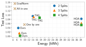
Figure 10: Compare test loss and energy consumption on activity set erckt.

This section provides more experimental results, including comprehensive results of performance evaluation and additional ablation studies.

C.1 Performance Evaluation

Table 3 and 5 provide comprehensive comparison of different methods on test loss and energy consumption on activity sets sdnkt and sdnkterca, respectively. They complement the results in Figure 2. Besides, Table 4 and Figure 10 compares these methods on activity set erckt. The results on erckt is similar to results on the other activity sets; our method achieves the best performance with around 40% less energy consumption than the one-by-one method and with slightly more energy consumption than all-in-one methods.

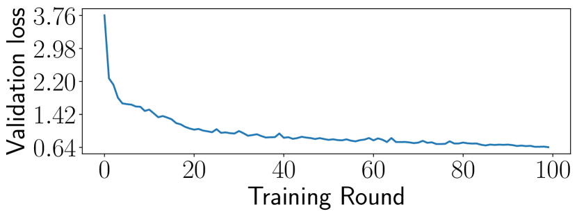
(a) Activity set sdnkt

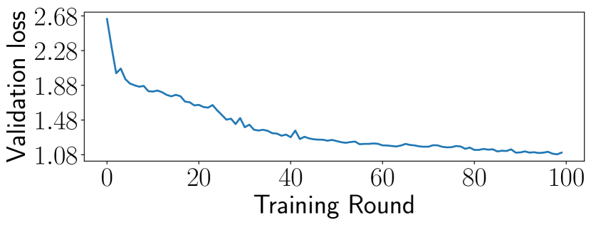
(b) Activity set erckt

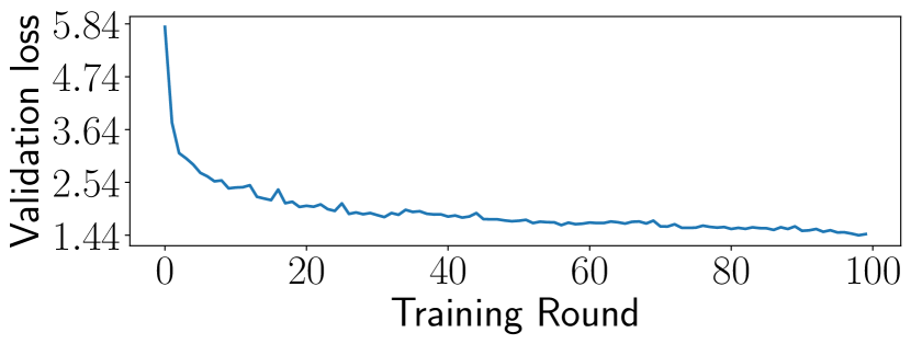
(c) Activity set sdnkterca

Figure 11: Changes of validation loss over the course of training on activity sets: (a) sdnkt, (b) erckt, and (c) sdnkterca. Validation loss converges as training proceeds.

Table 6: Activity splitting results of TAG [16] and MuFL on activity sets sdnkt, erckt, and sdnkterca. Activities of each split is separated by a comma.

Method	Activity Set	Two Splits	Three Splits	Four Splits	Five Splits
TAG	sdnkt	sdn,kt	sd,dn,kt	sd,sdn,dn,kt	-
MuFL	sdnkt	sdn,kt	sdn,k,t	sd,n,k,t	s,d,n,k,t
TAG	erckt	er,rckt	er,kt,rc	er,kt,rc,rt	-
MuFL	erckt	er,ckt	er,c,kt	er,c,k,t	e,r,c,k,t
TAG	sdnkterca	sdnkterca,dr	sdnerc,dr,kta	sc,dr,ne,kta	-
MuFL	sdnkterca	snkteac,dr	snec,dr,kta	sn,dr,ka,etc	sn,dr,ka,e,tc

Additionally, Table 3, 4 and 5 also provide carbon footprints (CO2eq) of different methods. The carbon footprints are estimated using Carbontracker [1]. Our method reduces around 40% on carbon footprints on these three activity sets compared with one-by-one training; it reduces 1526gCO₂eq or equivalent to traveling 12.68km by car on sdnkterca. The reduction is even more significant when compared with TAG and HOA. Although we run experiments using Tesla V100 GPU, the relative results of energy and carbon footprint among different methods should be representative of the scenarios of edge devices.

Table 7: Results of the optimal and worst splits in three runs of experiments. They are not identical due to variances in three runs of experiments.

Activity Set	Splits	Optimal Splits			Worst Splits
sdnkt	2	dk,snt	sn,dkt	nt,sdk	st,dnk	st,dnk	st,dnk
	3	t,sn,dk	k,t,sdn	d,sn,kt	d,st,nk	d,st,nk	s,dt,nk
erckt	2	r,eckt	t,erck	et,rck	rk,ect	ek,rct	e,rckt
	3	r,ec,kt	r,t,eck	r,ec,kt	c,e,rk	e,k,rct	e,rt,ck

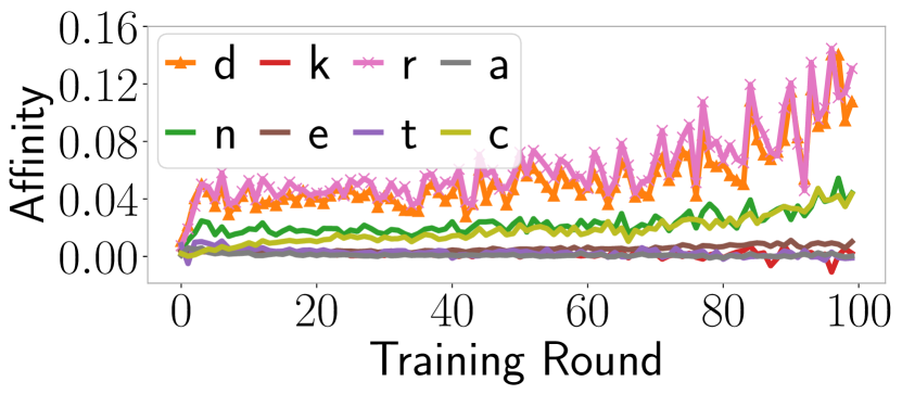
(a) Affinities to activity s

(b) Affinities to activity d

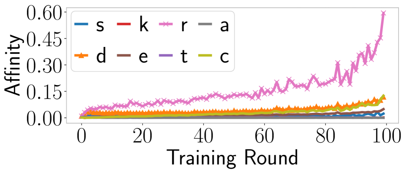
(c) Affinities to activity n

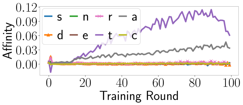
(d) Affinities to activity k

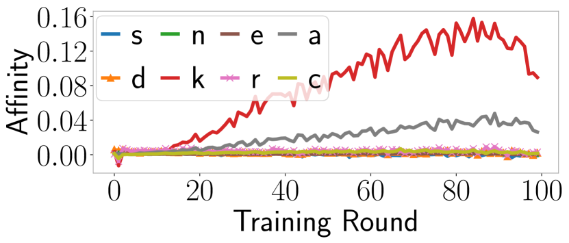
(e) Affinities to activity t

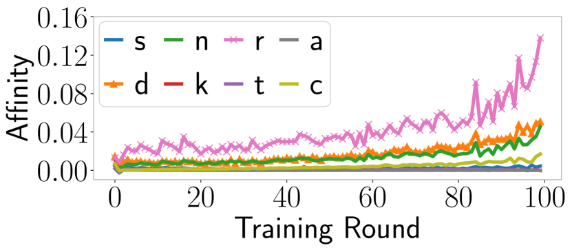
(f) Affinities to activity e

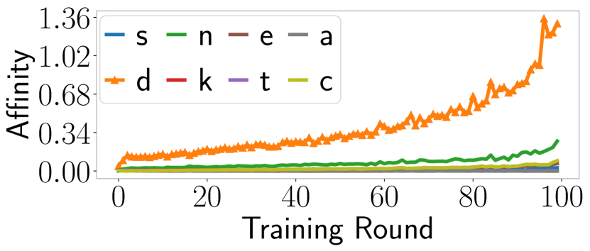
(g) Affinities to activity r

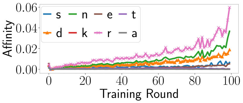
(h) Affinities to activity c

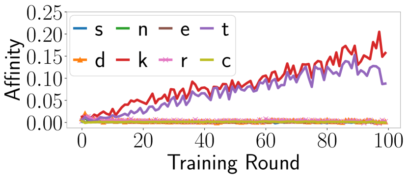
(i) Affinities to activity a

Figure 12: Changes of affinity scores of one activity to the other over the course of training on activity set sdnkterca. The trends of affinities emerge at the early stage of training.

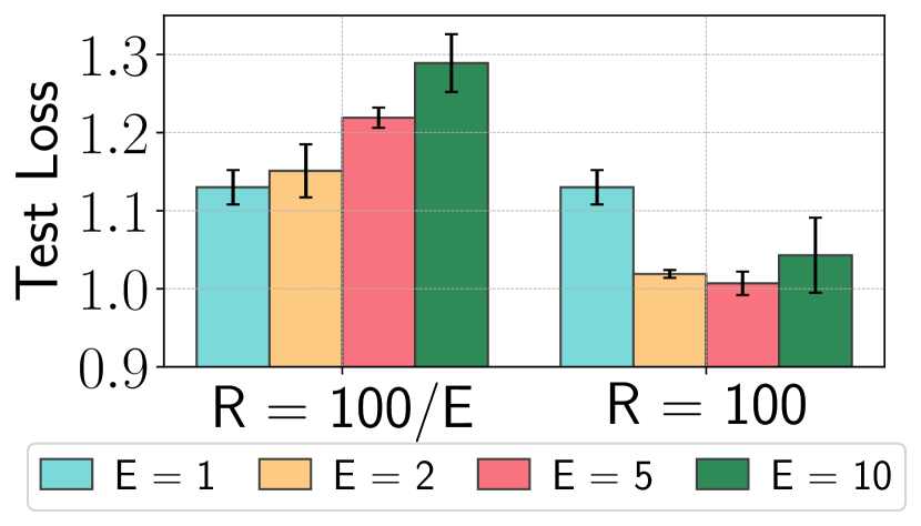
(a) Impact of $E$ on erckt

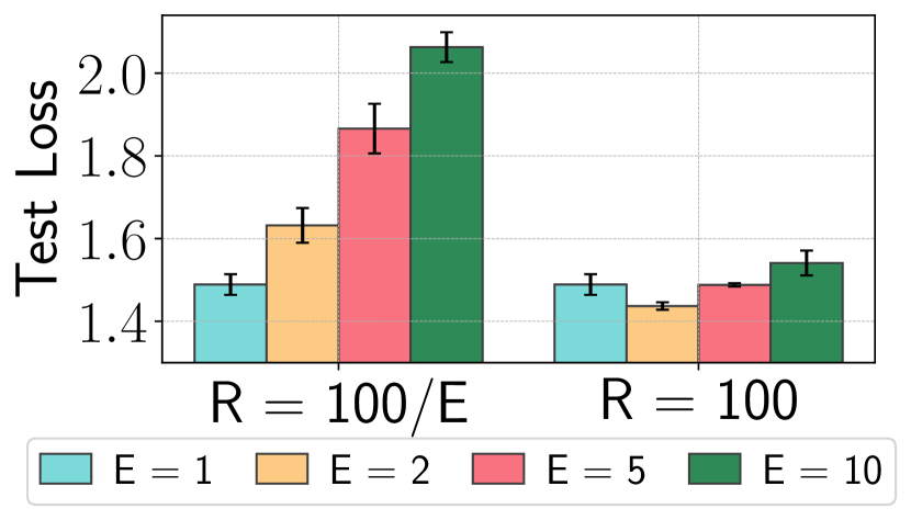
(b) Impact of $E$ on sdnkterca

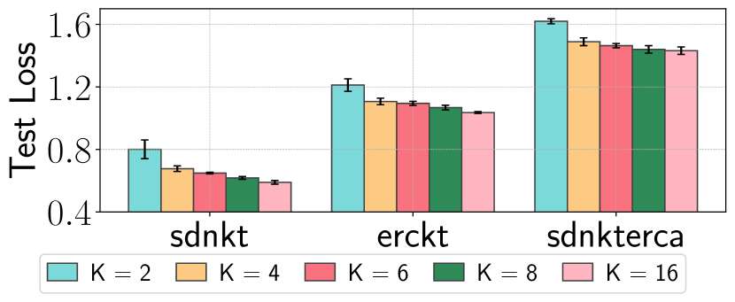
(c) Impact of $K$

Figure 13: Ablation studies on the impact of local epoch $E$ and impact of the number of selected clients $K$. Larger $E$ degrades performance when $R=\nicefrac{{100}}{{E}}$, but it could reduce losses when $R=100$. Larger $E$ (with $R=100$) and $K$ requires higher computation. They could reduce losses, but the marginal benefit decreases as computation increases.

C.2 Additional Analysis and Ablation Studies

This section presents additional analysis of MuFL and provides additional ablation studies.

Changes of Vadiation Loss

Figure 11 presents validation losses over the course of all-in-one training of three training activity sets sdnkt, erckt, and sdnkterca. It shows that validation losses converge as training proceeds.

Splitting Results of Various Methods

We provide results of activity splitting of TAG [16] and MuFL in Table 6. For hierarchical splitting, they further split into three splits from the results of two splits. In particular, the results of hierarchical splitting of erckt and sdnkterca are the same as their three splits. The hierarchical splitting result of sdnkt is from {sdn,kt} to {sd,n,kt} as the hierarchical splitting further divides the split with more training activities (sdn).

Besides, Table 7 presents the splitting results of the optimal and worst splits. They are not identical due to variances in multiple runs of experiments. We report the mean and standard deviation of test losses of the optimal splits and the worst splits in Table 1. The large variances of the optimal and worst splits suggest the instability of splitting by measuring the performances of training from scratch in the FL settings and show the advantage of our methods in obtaining stable splits.

Table 8: Comparison of test loss using different numbers of selected clients $K$. MuFL achieves even better performance on $K=8$.

	K	Total Loss	s	d	n	k	t
All-in-one	4	0.677	0.087	0.246	0.136	0.126	0.083
All-in-one	8	0.618	0.076	0.227	0.130	0.109	0.077
MuFL (two splits)	4	0.578	0.069	0.231	0.124	0.102	0.052
MuFL (two splits)	8	0.512	0.060	0.202	0.117	0.083	0.048

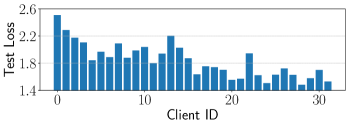
(a)

Methods	Test Loss
Standalone	1.842 ± 0.248
All-in-one	0.677 ± 0.018
MuFL	0.548 ± 0.001

(b)

Figure 14: Performance (test loss) of standalone training that conducts training using data in each client independently: (a) shows the test loss distribution of these thirty-two clients. (b) compares test losses of standalone training and FL methods. We run the experiments on activity set sdnkt.

Dataset Size and Performance

The dataset size of activity set sdnkt is around 315GB in our experiments, compared to 2.4TB of dataset used in experiments of TAG [16]. The test loss of ours (0.512 in Table 8), however, is better than the optimal one in TAG [16] (0.5246). This back-of-the-envelope comparison indicates the potential to extend our approaches to multi-task learning. Besides, it could also suggest that our data size is sufficient for evaluation.

Impact of Affinity Computation Frequency $f$

The frequency of computing affinities in Equation 2 determines the amount of extra needed computation. We use $f=5$ and compute affinities for the first ten rounds for all experiments because the trend of affinities emerge in the early stage of training in Figure 12. It would increase the computation of all-in-one training by around 2%, which is already factored into the energy consumption computation in previous experiments. The results in Table 3, 4, and 5 show that MuFL is effective with this setting and the amount of computation is acceptable.

Impact of Local Epoch

Figure 13(a) and 13(b) show the impact of local epoch $E$ on activity sets erckt and sdnkterca, respectively. They complement results of activity set sdnkt in Figure 5(a). On the one hand, larger $E$ degrades performance when $R=\nicefrac{{100}}{{E}}$, even though the total computation remains. It could be due to the impact of statistical heterogeneity; larger $E$ amplifies the heterogeneity among selected clients. On the other hand, larger $E$ could lead to better performance when fixing $R=100$. It is especially effective when increasing $E=1$ to $E=2$, but further increasing $E$ could degrade the performance. It indicates that simply increasing computation has limited capability to improve the performance.

Impact of The Number of Selected Clients

Figure 13(c) compares the performance of different numbers of selected clients $K=\{2,4,6,8,16\}$ on three activity sets sdnkt, erckt, and sdnkterca. It complements results in Figure 5(b). The results on three activity sets are similar; increasing $K$ reduces losses, but the marginal benefit decreases as $K$ increases.

The majority of experiments in this study are conducted with $K=4$. We next analyze the impact of $K$ in MuFL with results of two splits on activity set sdnkt in Table 8. The results indicate that MuFL is still effective with $K=8$, which outperforms $K=4$ and all-in-one training.

Standalone Training

Standalone training refers to training using data of each client independently. Figure 14(a) shows the test loss distribution of thirty-two clients used in experiments. The client ID corresponds to the dataset size distribution in Figure 7. These results suggest that larger data sizes of clients may not lead to higher performance. Figure 14(b) compares test losses of standalone training and federated learning methods. Either all-in-one or our MuFL greatly outperforms standalone training. It suggests the significance of federated learning when data are not sharable among clients.

Appendix D Algorithm

Algorithm 1 Our Proposed Smart Multi-tenant FL System (MuFL)

1:Input: training activities $\mathcal{A}=\{\alpha_{1},\alpha_{2},\dots,\alpha_{n}\}$, a set of available clients $\mathcal{C}$, number of selected clients $K$, local epoch $E$, aggregation weight of client $k$ $p_{k}$, total training rounds $R$, all-in-one training rounds $R_{0}$, frequency of computing affinities $f$, batch size $B$

2:Output: models $\mathcal{W}=\{\omega_{1},\omega_{2},\dots,\omega_{n}\}$

3:

4:ServerExecution:

5:Consolidate $\mathcal{A}$ into $\alpha_{0}$ with a multi-task model $\nu^{0}=\{\theta_{s}\}\cup\{\theta_{\alpha_{i}}|\alpha_{i}\in\mathcal{A}\}$

6:Initialize $\nu^{0}$, i.e. initialize $\omega_{i}=\{\theta_{s}\}\cup\{\theta_{\alpha_{i}}\}$ for $i\in\mathcal{N}=\{1,2,\dots,n\}$

7:for each round $r=0,1,...,R_{0}-1$ do

8:     $\mathcal{C}^{r}\leftarrow$ (Randomly select K clients from $\mathcal{C}$)

9:     for client $k\in\mathcal{C}^{r}$ in parallel do

10:         $\nu^{r,k},\hat{\mathcal{S}}_{\alpha_{i}\rightarrow\alpha_{j}}^{r,k}\leftarrow$Client($\nu^{r}$, $\mathcal{A}$, $f$)

11:     end for

12:     $\nu^{r+1}\leftarrow\sum\limits_{k\in\mathcal{C}^{r}}p_{k}\nu^{r,k}$

13:     $\hat{\mathcal{S}}^{r}_{\alpha_{i}\rightarrow\alpha_{j}}\leftarrow\frac{1}{K}\sum\limits_{k\in\mathcal{C}^{r}}\hat{\mathcal{S}}^{r,k}_{\alpha_{i}\rightarrow\alpha_{j}}$

14:end for

15:Compute the values of $\mathcal{S}^{r}_{\alpha_{i}\rightarrow\alpha_{i}}$, $\forall\alpha_{i}\in\mathcal{A}$, using Equation 3

16:Compute a set $I\subseteq\{1,2,3,...,m\}$ for splits $\{\mathcal{A}_{j}|j\in I\}$ using branch-and-bound algorithm and affinites $\mathcal{S}^{r}_{\alpha_{i}\rightarrow\alpha_{j}}$ ($\forall\alpha_{i}\in\mathcal{A}$ and $\forall\alpha_{j}\in\mathcal{A}$) to maximize $\mathcal{S}^{r}_{\alpha_{i}}$

17:for each element $j\in I$ do

18:     Initialize $\nu_{j}=\{\theta_{s}^{j}\}\cup\{\theta_{\alpha_{i}}|\alpha_{i}\in\mathcal{A}_{j}\}$ with parameters of $\nu^{R_{0}}$

19:     for each round $r=0,1,...,R-R_{0}-1$ do

20:         $\mathcal{C}^{r}\leftarrow$ (Random select K from $\mathcal{C}$)

21:         for client $k\in\mathcal{C}^{r}$ in parallel do

22:              $\nu_{j}^{r,k},$ _ $\leftarrow$Client($\nu_{j}^{r}$, $\mathcal{A}_{j}$, 0)

23:         end for

24:         $\nu_{j}^{r+1}\leftarrow\sum\limits_{k\in\mathcal{C}^{r}}p_{k}\nu_{j}^{r,k}$

25:     end for

26:end for

27:Reconstruct $\mathcal{W}=\{\omega_{1},\omega_{2},\dots,\omega_{n}\}$ from $\{\nu_{j}|j\in I\}$ by matching training activities

28:Return $\mathcal{W}$

29:

30:Client ($\nu$, $\mathcal{A}$, $f$):

31:$T=\lfloor\frac{B}{f}\rfloor$ if $f\neq 0$ else $0$

32:for local epoch $e=1,...,E$ do

33:     Update model parameters $\nu$ with respect to training activities $\mathcal{A}$

34:     for each time-step $t=1,2,...,T$ (every $f$ batches) do

35:         $\forall\alpha_{i}\in\mathcal{A}$ and $\forall\alpha_{j}\in\mathcal{A}$, compute affinities of $\mathcal{S}^{t}_{\alpha_{i}\rightarrow\alpha_{j}}$ using Equation 2

36:     end for

37:end for

38:$\hat{\mathcal{S}}_{\alpha_{i}\rightarrow\alpha_{j}}=\frac{1}{ET}\sum\limits_{e=1}^{E}\sum\limits_{t=1}^{T}\mathcal{S}^{t}_{\alpha_{i}\rightarrow\alpha_{j}}$, $\forall\alpha_{i}\in\mathcal{A}$ and $\forall\alpha_{j}\in\mathcal{A}$

39:Return $\nu$, $\hat{\mathcal{S}}_{\alpha_{i}\rightarrow\alpha_{j}}$

References

- [1] L. F. W. Anthony, B. Kanding, and R. Selvan. Carbontracker: Tracking and predicting the carbon footprint of training deep learning models. ICML Workshop on Challenges in Deploying and monitoring Machine Learning Systems, July 2020. arXiv:2007.03051.
- [2] E. Bagdasaryan, A. Veit, Y. Hua, D. Estrin, and V. Shmatikov. How to backdoor federated learning. In International Conference on Artificial Intelligence and Statistics, pages 2938–2948. PMLR, 2020.
- [3] H. Bilen and A. Vedaldi. Integrated perception with recurrent multi-task neural networks. Advances in neural information processing systems, 29, 2016.
- [4] K. Bonawitz, H. Eichner, W. Grieskamp, D. Huba, A. Ingerman, V. Ivanov, C. Kiddon, J. Konečnỳ, S. Mazzocchi, B. McMahan, et al. Towards federated learning at scale: System design. Proceedings of Machine Learning and Systems, 1:374–388, 2019.
- [5] H. Cai, B. Reinwald, N. Wang, and C. J. Guo. Saas multi-tenancy: Framework, technology, and case study. In Cloud Computing Advancements in Design, Implementation, and Technologies, pages 67–82. IGI Global, 2013.
- [6] R. Caruana. Multitask learning. Machine learning, 28(1):41–75, 1997.
- [7] Z. Chai, A. Ali, S. Zawad, S. Truex, A. Anwar, N. Baracaldo, Y. Zhou, H. Ludwig, F. Yan, and Y. Cheng. Tifl: A tier-based federated learning system. In Proceedings of the 29th International Symposium on High-Performance Parallel and Distributed Computing, pages 125–136, 2020.
- [8] Z. Chen, V. Badrinarayanan, C.-Y. Lee, and A. Rabinovich. Gradnorm: Gradient normalization for adaptive loss balancing in deep multitask networks. In International Conference on Machine Learning, pages 794–803. PMLR, 2018.
- [9] F. Chollet. Xception: Deep learning with depthwise separable convolutions. In Proceedings of the IEEE conference on computer vision and pattern recognition, pages 1251–1258, 2017.
- [10] F. Chong and G. Carraro. Architecture strategies for catching the long tail. MSDN Library, Microsoft Corporation, 910, 2006.
- [11] M. Dowty and J. Sugerman. Gpu virtualization on vmware’s hosted i/o architecture. ACM SIGOPS Operating Systems Review, 43(3):73–82, 2009.
- [12] L. Duong, T. Cohn, S. Bird, and P. Cook. Low resource dependency parsing: Cross-lingual parameter sharing in a neural network parser. In Proceedings of the 53rd annual meeting of the Association for Computational Linguistics and the 7th international joint conference on natural language processing (volume 2: short papers), pages 845–850, 2015.
- [13] D. Eigen and R. Fergus. Predicting depth, surface normals and semantic labels with a common multi-scale convolutional architecture. In Proceedings of the IEEE international conference on computer vision, pages 2650–2658, 2015.
- [14] B. Fang, X. Zeng, and M. Zhang. Nestdnn: Resource-aware multi-tenant on-device deep learning for continuous mobile vision. In Proceedings of the 24th Annual International Conference on Mobile Computing and Networking, pages 115–127, 2018.
- [15] C. Fehling, F. Leymann, and R. Mietzner. A framework for optimized distribution of tenants in cloud applications. In 2010 IEEE 3rd International Conference on Cloud Computing, pages 252–259. IEEE, 2010.
- [16] C. Fifty, E. Amid, Z. Zhao, T. Yu, R. Anil, and C. Finn. Efficiently identifying task groupings for multi-task learning. Advances in Neural Information Processing Systems, 34, 2021.
- [17] P. Guo, C.-Y. Lee, and D. Ulbricht. Learning to branch for multi-task learning. In International Conference on Machine Learning, pages 3854–3863. PMLR, 2020.
- [18] A. Hard, K. Rao, R. Mathews, S. Ramaswamy, F. Beaufays, S. Augenstein, H. Eichner, C. Kiddon, and D. Ramage. Federated learning for mobile keyboard prediction. arXiv preprint arXiv:1811.03604, 2018.
- [19] F. Hartmann, S. Suh, A. Komarzewski, T. D. Smith, and I. Segall. Federated learning for ranking browser history suggestions. arXiv preprint arXiv:1911.11807, 2019.
- [20] C.-H. Hong, I. Spence, and D. S. Nikolopoulos. Gpu virtualization and scheduling methods: A comprehensive survey. ACM Computing Surveys (CSUR), 50(3):1–37, 2017.
- [21] S. Huang, X. Li, Z.-Q. Cheng, Z. Zhang, and A. Hauptmann. Gnas: A greedy neural architecture search method for multi-attribute learning. In Proceedings of the 26th ACM international conference on Multimedia, pages 2049–2057, 2018.
- [22] Y. Huang, S. Gupta, Z. Song, K. Li, and S. Arora. Evaluating gradient inversion attacks and defenses in federated learning. Advances in Neural Information Processing Systems, 34, 2021.
- [23] J. Janai, F. Güney, A. Behl, A. Geiger, et al. Computer vision for autonomous vehicles: Problems, datasets and state of the art. Foundations and Trends® in Computer Graphics and Vision, 12(1–3):1–308, 2020.
- [24] M. Jeon, S. Venkataraman, A. Phanishayee, J. Qian, W. Xiao, and F. Yang. Analysis of Large-Scale Multi-Tenant GPU clusters for DNN training workloads. In 2019 USENIX Annual Technical Conference (USENIX ATC 19), pages 947–960, Renton, WA, July 2019. USENIX Association.
- [25] A. H. Jiang, D. L.-K. Wong, C. Canel, L. Tang, I. Misra, M. Kaminsky, M. A. Kozuch, P. Pillai, D. G. Andersen, and G. R. Ganger. Mainstream: Dynamic Stem-Sharing for Multi-Tenant video processing. In 2018 USENIX Annual Technical Conference (USENIX ATC 18), pages 29–42, 2018.
- [26] P. Kairouz, H. B. McMahan, B. Avent, A. Bellet, M. Bennis, A. N. Bhagoji, K. Bonawitz, Z. Charles, G. Cormode, R. Cummings, et al. Advances and open problems in federated learning. Foundations and Trends® in Machine Learning, 14(1–2):1–210, 2021.
- [27] Z. Kang, K. Grauman, and F. Sha. Learning with whom to share in multi-task feature learning. In ICML, 2011.
- [28] S. P. Karimireddy, S. Kale, M. Mohri, S. Reddi, S. Stich, and A. T. Suresh. Scaffold: Stochastic controlled averaging for federated learning. In International Conference on Machine Learning, pages 5132–5143. PMLR, 2020.
- [29] A. Kendall, Y. Gal, and R. Cipolla. Multi-task learning using uncertainty to weigh losses for scene geometry and semantics. In Proceedings of the IEEE conference on computer vision and pattern recognition, pages 7482–7491, 2018.
- [30] J. Konečný, H. B. McMahan, F. X. Yu, P. Richtarik, A. T. Suresh, and D. Bacon. Federated learning: Strategies for improving communication efficiency. In NIPS Workshop on Private Multi-Party Machine Learning, 2016.
- [31] R. Krebs, C. Momm, and S. Kounev. Architectural concerns in multi-tenant saas applications. Closer, 12:426–431, 2012.
- [32] A. Kumar and H. Daumé. Learning task grouping and overlap in multi-task learning. In Proceedings of the 29th International Coference on International Conference on Machine Learning, page 1723–1730, 2012.
- [33] C. Lao, Y. Le, K. Mahajan, Y. Chen, W. Wu, A. Akella, and M. Swift. ATP: In-network aggregation for multi-tenant learning. In 18th USENIX Symposium on Networked Systems Design and Implementation (NSDI 21), pages 741–761. USENIX Association, Apr. 2021.
- [34] E. L. Lawler and D. E. Wood. Branch-and-bound methods: A survey. Operations research, 14(4):699–719, 1966.
- [35] T. Li, A. K. Sahu, M. Zaheer, M. Sanjabi, A. Talwalkar, and V. Smith. Federated optimization in heterogeneous networks. Proceedings of Machine Learning and Systems, 2:429–450, 2020.
- [36] W. Li, F. Milletarì, D. Xu, N. Rieke, J. Hancox, W. Zhu, M. Baust, Y. Cheng, S. Ourselin, M. J. Cardoso, et al. Privacy-preserving federated brain tumour segmentation. In International Workshop on Machine Learning in Medical Imaging, pages 133–141. Springer, 2019.
- [37] J. Liu, J. Liu, W. Du, and D. Li. Performance analysis and characterization of training deep learning models on mobile device. In 2019 IEEE 25th International Conference on Parallel and Distributed Systems (ICPADS), pages 506–515. IEEE, 2019.
- [38] Y. Lu, A. Kumar, S. Zhai, Y. Cheng, T. Javidi, and R. Feris. Fully-adaptive feature sharing in multi-task networks with applications in person attribute classification. In Proceedings of the IEEE conference on computer vision and pattern recognition, pages 5334–5343, 2017.
- [39] O. Marfoq, G. Neglia, A. Bellet, L. Kameni, and R. Vidal. Federated multi-task learning under a mixture of distributions. Advances in Neural Information Processing Systems, 34, 2021.
- [40] B. McMahan, E. Moore, D. Ramage, S. Hampson, and B. A. y Arcas. Communication-efficient learning of deep networks from decentralized data. In Artificial intelligence and statistics, pages 1273–1282. PMLR, 2017.
- [41] R. Mietzner, F. Leymann, and M. P. Papazoglou. Defining composite configurable saas application packages using sca, variability descriptors and multi-tenancy patterns. In 2008 third international conference on Internet and web applications and services, pages 156–161. IEEE, 2008.
- [42] L. Minto, M. Haller, B. Livshits, and H. Haddadi. Stronger privacy for federated collaborative filtering with implicit feedback. In Fifteenth ACM Conference on Recommender Systems, pages 342–350, 2021.
- [43] I. Misra, A. Shrivastava, A. Gupta, and M. Hebert. Cross-stitch networks for multi-task learning. In Proceedings of the IEEE conference on computer vision and pattern recognition, pages 3994–4003, 2016.
- [44] V. Nekrasov, T. Dharmasiri, A. Spek, T. Drummond, C. Shen, and I. Reid. Real-time joint semantic segmentation and depth estimation using asymmetric annotations. In 2019 International Conference on Robotics and Automation (ICRA), pages 7101–7107. IEEE, 2019.
- [45] A. Nguyen, T. Do, M. Tran, B. X. Nguyen, C. Duong, T. Phan, E. Tjiputra, and Q. D. Tran. Deep federated learning for autonomous driving. arXiv preprint arXiv:2110.05754, 2021.
- [46] A. Paszke, S. Gross, S. Chintala, G. Chanan, E. Yang, Z. DeVito, Z. Lin, A. Desmaison, L. Antiga, and A. Lerer. Automatic differentiation in pytorch. 2017.
- [47] J. Posner, L. Tseng, M. Aloqaily, and Y. Jararweh. Federated learning in vehicular networks: opportunities and solutions. IEEE Network, 35(2):152–159, 2021.
- [48] S. Ramaswamy, R. Mathews, K. Rao, and F. Beaufays. Federated learning for emoji prediction in a mobile keyboard. arXiv preprint arXiv:1906.04329, 2019.
- [49] M. J. Sheller, G. A. Reina, B. Edwards, J. Martin, and S. Bakas. Multi-institutional deep learning modeling without sharing patient data: A feasibility study on brain tumor segmentation. In International MICCAI Brainlesion Workshop, pages 92–104. Springer, 2018.
- [50] V. Smith, C.-K. Chiang, M. Sanjabi, and A. S. Talwalkar. Federated multi-task learning. Advances in neural information processing systems, 30, 2017.
- [51] T. Standley, A. Zamir, D. Chen, L. Guibas, J. Malik, and S. Savarese. Which tasks should be learned together in multi-task learning? In International Conference on Machine Learning, pages 9120–9132. PMLR, 2020.
- [52] X. Sun, R. Panda, R. Feris, and K. Saenko. Adashare: Learning what to share for efficient deep multi-task learning. Advances in Neural Information Processing Systems, 33:8728–8740, 2020.
- [53] S. Thrun. Is learning the n-th thing any easier than learning the first? Advances in neural information processing systems, 8, 1995.
- [54] S. Vandenhende, S. Georgoulis, B. De Brabandere, and L. Van Gool. Branched multi-task networks: deciding what layers to share. arXiv preprint arXiv:1904.02920, 2019.
- [55] H. Wang, M. Yurochkin, Y. Sun, D. Papailiopoulos, and Y. Khazaeni. Federated learning with matched averaging. In International Conference on Learning Representations, 2020.
- [56] J. Wang, Q. Liu, H. Liang, G. Joshi, and H. V. Poor. Tackling the objective inconsistency problem in heterogeneous federated optimization. arXiv preprint arXiv:2007.07481, 2020.
- [57] C. Yang, Q. Wang, M. Xu, Z. Chen, K. Bian, Y. Liu, and X. Liu. Characterizing impacts of heterogeneity in federated learning upon large-scale smartphone data. In Proceedings of the Web Conference 2021, pages 935–946, 2021.
- [58] T. Yang, G. Andrew, H. Eichner, H. Sun, W. Li, N. Kong, D. Ramage, and F. Beaufays. Applied federated learning: Improving google keyboard query suggestions. arXiv preprint arXiv:1812.02903, 2018.
- [59] T. Yu, S. Kumar, A. Gupta, S. Levine, K. Hausman, and C. Finn. Gradient surgery for multi-task learning. Advances in Neural Information Processing Systems, 33:5824–5836, 2020.
- [60] yuyang deng, M. M. Kamani, and M. Mahdavi. Adaptive personalized federated learning, 2021.
- [61] A. R. Zamir, A. Sax, W. Shen, L. J. Guibas, J. Malik, and S. Savarese. Taskonomy: Disentangling task transfer learning. In Proceedings of the IEEE conference on computer vision and pattern recognition, pages 3712–3722, 2018.
- [62] H. Zhang, J. Bosch, and H. H. Olsson. End-to-end federated learning for autonomous driving vehicles. In 2021 International Joint Conference on Neural Networks (IJCNN), pages 1–8. IEEE, 2021.
- [63] J. Zhang, S. Guo, X. Ma, H. Wang, W. Xu, and F. Wu. Parameterized knowledge transfer for personalized federated learning. Advances in Neural Information Processing Systems, 34, 2021.
- [64] Y. Zhang and Q. Yang. A survey on multi-task learning. IEEE Transactions on Knowledge and Data Engineering, 2021.
- [65] H. Zhao, Z. Han, Z. Yang, Q. Zhang, F. Yang, L. Zhou, M. Yang, F. C. Lau, Y. Wang, Y. Xiong, and B. Wang. HiveD: Sharing a GPU cluster for deep learning with guarantees. In 14th USENIX Symposium on Operating Systems Design and Implementation (OSDI 20), pages 515–532. USENIX Association, Nov. 2020.
- [66] X. Zhao, H. Li, X. Shen, X. Liang, and Y. Wu. A modulation module for multi-task learning with applications in image retrieval. In Proceedings of the European Conference on Computer Vision (ECCV), pages 401–416, 2018.
- [67] L. Zhu, H. Lin, Y. Lu, Y. Lin, and S. Han. Delayed gradient averaging: Tolerate the communication latency for federated learning. Advances in Neural Information Processing Systems, 34, 2021.
- [68] W. Zhuang, X. Gan, Y. Wen, and S. Zhang. Easyfl: A low-code federated learning platform for dummies. IEEE Internet of Things Journal, 2022.
- [69] W. Zhuang, X. Gan, Y. Wen, and S. Zhang. Optimizing performance of federated person re-identification: Benchmarking and analysis. ACM Transactions on Multimedia Computing, Communications, and Applications (TOMM), 2022.
- [70] W. Zhuang, X. Gan, Y. Wen, S. Zhang, and S. Yi. Collaborative unsupervised visual representation learning from decentralized data. In Proceedings of the IEEE/CVF International Conference on Computer Vision, pages 4912–4921, 2021.
- [71] W. Zhuang, Y. Wen, and S. Zhang. Joint optimization in edge-cloud continuum for federated unsupervised person re-identification. In Proceedings of the 29th ACM International Conference on Multimedia, pages 433–441, 2021.
- [72] W. Zhuang, Y. Wen, and S. Zhang. Divergence-aware federated self-supervised learning. In International Conference on Learning Representations, 2022.
- [73] W. Zhuang, Y. Wen, X. Zhang, X. Gan, D. Yin, D. Zhou, S. Zhang, and S. Yi. Performance optimization of federated person re-identification via benchmark analysis. In Proceedings of the 28th ACM International Conference on Multimedia, pages 955–963, 2020.