Condensation and Evaporation of Boson Stars

Abstract

Axion-like particles, including the QCD axion, are well-motivated dark matter candidates. Numerical simulations have revealed coherent soliton configurations, also known as boson stars, in the centers of axion halos. We study evolution of axion solitons immersed into a gas of axion waves with Maxwellian velocity distribution. Combining analytical approach with controlled numerical simulations we find that heavy solitons grow by condensation of axions from the gas, while light solitons evaporate. We deduce the parametric dependence of the soliton growth/evaporation rate and show that it is proportional to the rate of the kinetic relaxation in the gas. The proportionality coefficient is controlled by the product of the soliton radius and the typical gas momentum or, equivalently, the ratio of the gas and soliton virial temperatures. We discuss the asymptotics of the rate when this parameter is large or small.

1 Introduction

QCD axion [1, 2, 3, 4, 5, 6, 7, 8, 9] and axion-like particles [10, 11, 12, 13], are widely discussed in the literature as well-motivated dark matter (DM) candidates. The QCD axion, originally suggested as a solution to the strong CP problem [14, 15], was soon realized [7] to be produced in the early universe and behave as cold dark matter after the QCD phase transition endowing it with the mass. The requirement that the QCD axion accounts for all of DM leads to a preferred mass window $m_{aQCD}\sim 10^{-6}\div 10^{-4}~{}{\rm eV}$.

Axion-like particles with broad range of masses and very weak coupling to the Standard Model naturally arise in many beyond Standard Model scenarios and string theory [16, 10]. For brevity, we will refer to DM made of such particles as axion DM. Particularly interesting is the case of ultralight (also called “fuzzy”) DM with mass $m_{a}\sim 10^{-22}\div 10^{-19}~{}{\rm eV}$ [17]. The de Broglie wavelength of such ultralight particle corresponding to virial velocity in a galactic halo,

$$\lambda_{a}=\frac{2\pi}{mv_{a}}\sim\,1.2\times\,\left(\frac{m_{a}}{10^{-22}\,\mathrm{eV}}\right)^{-1}\,\left(\frac{v_{a}}{100\,\mathrm{km/s}}\right)^{-1}\mathrm{kpc}\ ,$$ (1.1)

is comparable to the typical cosmological and astrophysical distances. Due to this property, ultralight dark matter exhibits rich phenomenology affecting various cosmological observables and galactic dynamics [11, 12, 13]. The analysis of Lyman-$\alpha$ forest [18, 19, 20], galactic rotation curves [21, 22], halo profiles of dwarf galaxies [23, 24] and subhalo population in the Milky Way [25] strongly disfavor DM lighter than $10^{-21}~{}{\rm eV}$. Dynamical heating of stars by ultralight DM in ultrafaint dwarf galaxies has been used to infer tighter constraints ${m_{a}\gtrsim 10^{-19}~{}{\rm eV}}$ [26, 27].

A distinctive feature of axion DM is its huge occupation numbers (phase-space density) which are allowed because axions are bosons,

$$f_{\textbf{k}}\sim 10^{86}\times\left(\frac{\rho_{a}}{0.3\,{\rm GeV/cm}^{3}}\right)\,\left(\frac{m_{a}}{10^{-20}\,\mathrm{eV}}\right)^{-4}\,\left(\frac{v_{a}}{100\,{\rm km/s}}\right)^{-3}\ .$$ (1.2)

This implies that, rather than behaving as a collection of individual particles, axion DM is best described by a coherent classical scalar field with the scattering rate of axions increased due to the Bose enhancement. Typically, in the study of structure formation all axion interactions besides gravity can be neglected resulting in a universal wave dynamics described by Schrödinger–Poisson equations [13]. The dependence of these equations on the axion mass can be taken into account by a simple rescaling, and thus they apply to any axion DM as long as $f_{\bf k}\gg 1$.

The Schrödinger–Poisson system admits a spherically symmetric localized solution known as axion soliton or boson star [28]. All axions comprising the soliton are in the same state which is the ground state of the gravitational potential and hence the soliton can be viewed as inhomogeneous Bose–Einstein condensate sustained by its own gravity [29]. Numerical simulations of axion DM have revealed formation of boson stars in the centers of virialized axion halos (also known as miniclusters [30, 31] in the case of QCD axion). This phenomenon was observed in the cosmological setting [32, 33, 34, 35], in numerical experiments with halos created by collisions of several seed solitons [36, 37, 38], and in the kinetic relaxation regime [39]. It was also found that if the soliton is artificially removed from the halo, evolution readily reinstates it back [40].

Thus, presence of a solitonic core appears to be a generic feature of an axion halo. The rest of the halo represents a cloud of randomly moving wavepackets with the velocities roughly following the Maxwellian distribution and the average density fitted by the NFW profile [41], similarly to the usual cold DM. It is natural to ask how the soliton interacts with this environment. Refs. [42, 43, 44, 45] showed that interference between the soliton and wavepackets leads to oscillations of its density and to a random walk of the soliton center around the halo center of mass. Further, an interesting correlation between the soliton mass and the mass of its host halo has been established in cosmological numerical simulations [32, 36] and confirmed in [33, 42]. This relation can be rephrased as equality between the virial temperatures of the soliton and the host halo. While this relation may appear intuitive, the physical mechanism behind it remains unclear. It is not reproduced by simulations starting from non-cosmological initial conditions [37, 38, 46], whereas more recent cosmological simulations [47, 35, 46] indicate that it is subject to a large scatter, perhaps due to different merger histories of different halos. The results of Ref. [39] disfavor a potential interpretation of the soliton-host halo relation as a condition for kinetic equilibrium. Indeed, it was observed that, once formed, the solitons continue to grow by condensation of axions from the surrounding gas. On the other hand, Refs. [42, 48] argue that this growth slows down when the soliton becomes heavy enough to heat up the inner part of the halo and, given the finite time of the simulations, this can explain the observed correlation. The mass of the soliton can be also significantly affected by baryonic matter, typically leading to its increase [49, 50].

Boson stars give rise to important signatures opening up various opportunities for future discovery or constraints on axion DM. In the case of fuzzy DM, they are expected to play a prominent role in galactic dynamics modifying the rotation curves [21, 22] and heating the stars in the central regions through oscillations and random walk [26, 51, 52]. When axion self-interaction is included, they become unstable if their mass exceeds a certain threshold and collapse producing bursts of relativistic axions [53]. Further allowing for possible axion coupling to photons, they can be sources of radio emission [54, 55, 56]. Presence or absence of boson stars in axion miniclusters can have important implications for their density profiles and lensing searches [57, 58]. Very dense boson stars made of inflaton field get produced in inflationary models with delayed reheating opening a potentially rich phenomenology, such as seeding primordial black holes or contributing into stochastic high-frequency gravitational wave background [59].

The dynamical range achievable in axion DM simulations is severely limited by the computational costs (see the discussion in [35]). This calls for better theoretical understanding of the physical laws governing the evolution of boson stars in various environments which would allow their extrapolation outside of the parameter regions explored in simulations. In the present paper we make a step in this direction by studying the evolution of a boson star immersed in a box filled with homogeneous axion gas. Focusing on this setup allows us to get rid of the uncertainties related to the dynamics of the halo and keep under control the gas density and its velocity distribution. The latter is chosen to be Maxwellian at the initial moment of time. Similar setup was employed in Ref. [39] to study the formation of the soliton in the process of the gas kinetic relaxation. By contrast, we do not assume the soliton to be formed from the gas and simply add it in the initial conditions of our simulations. In this way we are able to explore a wide range of soliton masses corresponding different ratios between the soliton virial temperature $T_{s}$ and the temperature of the gas $T_{g}$.

The key quantity that we are interested in is the rate of change of the soliton mass,

$$\Gamma_{s}=\frac{1}{M_{s}}\frac{dM_{s}}{dt}\;.$$ (1.3)

We study the dependence of this quantity on the parameters characterizing the gas and the soliton by a combination of analytical and numerical methods. We find that the solitons with $T_{s}/T_{g}\gtrsim 0.1$ grow by absorbing particles from the gas. For fixed gas parameters, the growth rate is essentially constant in the range $0.1\lesssim T_{s}/T_{g}\lesssim 1$, whereas at $T_{s}/T_{g}\gtrsim 1$ it decreases as $(T_{s}/T_{g})^{-n/2}$ with $n=2\div 4$.

Interestingly, we find that if $T_{s}/T_{g}\lesssim 0.08$, the soliton evaporates, the time scale of this process being parametrically shorter than the relaxation time. This does not contradict previous results on soliton formation from the gas by kinetic relaxation [39]. Indeed, by running the simulations longer than the evaporation of the initial soliton we observe after a while the birth of a new soliton with $T_{s}/T_{g}\gtrsim 0.1$, in agreement with [39]. It is worth stressing the difference between the soliton evaporation and tidal disruption by large-scale gradients of the halo gravitational field [60]. This is clear already from the fact that there is no halo in our setup. Moreover, the qualitative direction of the process — evaporation vs. condensation — is entirely determined by the soliton and gas temperatures and does not depend on the density contrast between them.

The paper is organized as follows. In section 2 we introduce our framework and review the relevant properties of the soliton solution to the Schrödinger–Poisson equations. In section 3 we address the computation of the soliton growth/evaporation rate formulating it as a quantum-mechanical scattering problem. We consider separately the cases of light (cold, $T_{s}/T_{g}\ll 1$) and heavy (hot, $T_{s}/T_{g}\gg 1$) solitons and employ various approximations to estimate the rate analytically. In section 4 we describe our numerical simulations, extract the soliton growth rate from them and compare it to the analytic predictions. In section 5 we discuss the implications of our results and compare to other works. Three appendices contain auxiliary material. In appendix A we provide an alternative derivation of the soliton growth rate using only classical equations of motion. In appendix B we describe a suit of simulations reproducing the setup of Ref. [39] where the soliton forms from the gas spontaneously due to kinetic relaxation. Appendix C contains additional details about our numerical procedure.

2 Soliton Wavefunction and Axion Gas

Non-relativistic axions with mass $m$ are described by a complex scalar field $\psi$ obeying the Schrödinger–Poisson equations,

$$i\partial_{t}\psi+\frac{\Delta\psi}{2m}-m\Phi\psi=0\;,$$ (2.1a)

$$\Delta\Phi=4\pi Gm\,|\psi|^{2}\;,$$ (2.1b)

where $G$ is the gravitational coupling, $\Phi$ is the Newton potential and $\Delta$ denotes the Laplacian. The square of the field gives the particle number density, $|\psi(t,\mathbf{x})|^{2}=n(t,\mathbf{x})$. Equations (2.1) are invariant under scaling transformations,

$$\psi\mapsto\tilde{\psi}(t,\mathbf{x})=\Lambda_{3}\psi(\Lambda_{1}t,\Lambda_{2}\mathbf{x})\,,\qquad\Phi\mapsto\tilde{\Phi}(t,\mathbf{x})=\frac{\Lambda_{1}^{2}}{\Lambda_{2}^{2}}\Phi(\Lambda_{1}t,\Lambda_{2}\mathbf{x})\,,$$ (2.2a)

$$m\mapsto\tilde{m}=\frac{\Lambda_{2}^{2}}{\Lambda_{1}}m\,,\qquad G\mapsto\tilde{G}=\frac{\Lambda_{1}^{3}}{\Lambda_{2}^{2}\Lambda_{3}^{2}}G\,,$$ (2.2b)

where $\Lambda_{1,2,3}$ are arbitrary parameters. A one-parameter family of these transformations that leaves $m$ and $G$ invariant connects different solutions for a given axion; the transformations that change the mass, but not $G$, allow one to map between solutions for axions with different masses; finally, the rescaling of $G$ provides a freedom in the choice of units which is handy in numerical simulations.

The system (2.1) admits periodic spherically symmetric solutions of the form,

$$\psi_{s}(t,\mathbf{x})=\chi(|\mathbf{x}|){\rm e}^{-i{\cal E}_{s}t}\;.$$ (2.3)

The corresponding density $\rho_{s}(\mathbf{x})=m|\chi(|\mathbf{x}|)|^{2}$ is time-independent and localized in space, hence these solutions are called solitons. ${\cal E}_{s}$ represents the binding energy (chemical potential) of axions in the soliton and is negative. There is a continuous family of solitons differing by their mass $M_{s}$ and related by the subgroup of the scaling transformations (2.2) that leave $m$ and $G$ fixed. Using this symmetry, the soliton wavefunction can be written as

$$\chi(x)=\frac{k_{s}^{2}}{\sqrt{4\pi Gm^{3}}}\chi_{0}(k_{s}x)\;,$$ (2.4)

where $k_{s}$ is the scaling parameter characterizing the soliton width. By the uncertainty relation, it sets the typical momentum of particles comprising the soliton. The dimensionless function $\chi_{0}(\xi)$ describes the “standard soliton” normalized by the condition

$$\chi_{0}(0)=1\;.$$ (2.5a)

It solves the eigenvalue problem following from the Schrödinger–Poisson system,

$$\chi_{0}^{\prime\prime}+\frac{2}{\xi}\chi_{0}^{\prime}=2(\Phi_{0}-\varepsilon_{0})\chi_{0}\;,$$ (2.5b)

$$\Phi_{0}^{\prime\prime}+\frac{2}{\xi}\Phi_{0}^{\prime}=\chi_{0}^{2}\;,$$ (2.5c)

where $\Phi_{0}(\xi)$ is the standard soliton gravitational potential and $\varepsilon_{0}$ is its binding energy. Fig. 1 shows the function $\chi_{0}(\xi)$ obtained by numerically solving eqs. (2.5). It is well approximated by an analytic fit,

$$\chi_{0,{\rm fit}}=\big{(}1+c_{0}\xi^{2}\big{)}^{-4}~{},~{}~{}~{}~{}~{}~{}c_{0}=0.0539\;,$$ (2.6)

also shown in the figure. The fit differs from the exact solution only at the tail where the exact solution falls off exponentially, whereas the fit behaves as a power-law.

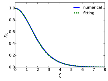
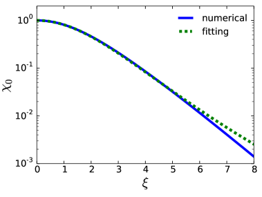
Figure 1: The standard soliton profile in linear (left) and in log (right) scale. The solid lines show the exact solution of the Schrödinger–Poisson equations, while the dotted lines correspond to the fitting function (2.6).

The standard soliton is characterized by the following dimensionless quantities:

$$\varepsilon_{0}=-0.692 \text{binding energy}\;,$$ (2.7a)

$$\mu_{0}=4\pi\int_{0}^{\infty}d\xi\,\xi^{2}\chi_{0}^{2}(\xi)=25.9 \text{total mass}\;,$$ (2.7b)

$$\xi_{0}=1.299 \text{half-density radius,}~{}|\chi_{0}(\xi_{0})|^{2}=1/2\;.$$ (2.7c)

The corresponding values for a general soliton are obtained by rescaling,

$${\cal E}_{s}=\varepsilon_{0}\frac{k_{s}^{2}}{m}~{},~{}~{}~{}~{}~{}~{}M_{s}=\mu_{0}\frac{k_{s}}{4\pi Gm^{2}}~{},~{}~{}~{}~{}~{}~{}r_{s}=\frac{\xi_{0}}{k_{s}}\;,$$ (2.8)

and its density profile can be approximated as

$$\rho_{s}({\bf x})\approx\frac{\rho_{s,\,{\rm peak}}}{\left[1+c_{s}\,\left(|{\bf x}|/r_{s}\right)^{2}\right]^{8}}~{},~{}~{}~{}~{}~{}\rho_{s,\,{\rm peak}}=\frac{k_{s}^{4}}{4\pi Gm^{2}}~{},~{}~{}c_{s}=0.091\;.$$ (2.9)

Note that the width of the soliton is inversely proportional to its mass. Accordingly, the peak density is proportional to the fourth power of the mass. The total energy of the soliton consists of kinetic and potential parts,

$$E_{s}=E_{s,{\rm kin}}+E_{s,{\rm pot}}=\int d^{3}x\left(\frac{|\nabla\psi_{s}|^{2}}{2m}+\frac{m\Phi_{s}|\psi_{s}|^{2}}{2}\right)\;.$$ (2.10)

Using the Schrödinger–Poisson equations one can show that they obey the virial theorem, $E_{s}=-E_{s,{\rm kin}}=E_{s,{\rm pot}}/2$, and

$$E_{s}=\frac{M_{s}\mathcal{E}_{s}}{3m}\;.$$ (2.11)

It is instructive to introduce the soliton virial temperature,

$$T_{s}=\frac{2mE_{s,{\rm kin}}}{3M_{s}}=-\frac{2}{9}\mathcal{E}_{s}\;.$$ (2.12)

Using eqs. (2.8) one obtains alternative expressions,

$$T_{s}=0.154\frac{k_{s}^{2}}{m}=\frac{0.259}{mr_{s}^{2}}\;.$$ (2.13)

We are interested to study how the mass of the soliton varies due to its interaction with a gas of axion waves. We assume the gas to fill a box of size

$$L\gg r_{s}\;.$$ (2.14)

Far away from the soliton, it is described by a collection of plane waves,

$$\psi_{g}(t,\mathbf{x})=\frac{1}{L^{3/2}}\sum_{\mathbf{k}}a_{\mathbf{k}}\,{\rm e}^{-i\frac{k^{2}}{2m}t+i\mathbf{k}\mathbf{x}}~{},~{}~{}~{}~{}~{}~{}~{}|\mathbf{x}|\gg r_{s}\;.$$ (2.15)

We choose the occupation numbers to follow the Maxwell distribution, consistent with the velocity distribution in a DM halo,

$$f_{\mathbf{k}}\equiv|a_{\mathbf{k}}|^{2}=f_{g}\,{\rm e}^{-k^{2}/k_{g}^{2}}\;,$$ (2.16)

where $k_{g}$ sets the characteristic momentum of particles in the gas. The normalization $f_{g}$ is related to the gas density as

$$f_{g}=\frac{(4\pi)^{3/2}}{mk_{g}^{3}}\rho_{g}\;.$$ (2.17)

Validity of the classical description requires $f_{g}\gg 1$. The phases of the amplitudes $a_{\mathbf{k}}$ are assumed to be random.

Using $k_{g}$ we can define an effective gas temperature,

$$T_{g}=\frac{k_{g}^{2}}{2m}\;.$$ (2.18)

To avoid confusion, we stress that this is not a true thermodynamic temperature since eq. 2.16 is not an equilibrium distribution of the boson gas which should follow the Bose–Einstein formula. However, the latter cannot be reached within the classical field theory. Rather, as demonstrated in Ref. [39], a homogeneous axion gas with initial distribution (2.16) will evolve towards the Rayleigh–Jeans occupation numbers diverging at low $k$. This relaxation proceeds on the time scale

$$\tau_{\rm rel}=\frac{\sqrt{2}b\,k_{g}^{6}}{12\pi^{3}G^{2}m^{3}\rho_{g}^{2}\,\mathop{\rm ln}\nolimits(k_{g}L)}\;,~{}~{}~{}~{}b\approx 0.9\;,$$ (2.19)

and culminates in the spontaneous formation of a soliton. We neglect the change of the gas distribution in our theoretical considerations and discuss the validity of this simplification later on. Numerically, we observe that the Maxwell distribution appears to get reinstated in the gas once the soliton is formed. Moreover, in the simulations where the soliton is present for the whole duration, the distribution remains close to Maxwellian at all moments of time.

Being a self-gravitating system, the homogeneous axion gas is unstable with respect to gravitational collapse leading to a halo formation. The corresponding Jeans length is

$$l_{J}=\frac{k_{g}}{m}\sqrt{\frac{\pi}{2G\rho_{g}}}\;,$$ (2.20)

where we have used that the sound speed in non-relativistic Maxwellian gas is $k_{g}/(\sqrt{2}m)$. We avoid this instability by considering the box size smaller than the Jeans length,

$$L<l_{J}\;.$$ (2.21)

Note that this condition is compatible with eq. 2.14 since $l_{J}$ can be made arbitrarily large by decreasing the gas density. In practice, however, eq. 2.21 imposes strong limitations on the numerical simulations, see section 4.

The total axion field describing a soliton immersed in the gas is given by the sum

$$\psi(t,\mathbf{x})=\psi_{s}(t,\mathbf{x})+\psi_{g}(t,\mathbf{x})\;.$$ (2.22)

For this decomposition to be well-defined, the number of particles in the soliton must be much larger than in any other state in the gas,

$$M_{s}/m\gg f_{\mathbf{k}}\;.$$ (2.23)

To compare the soliton size with the characteristic wavelength of axion waves, we introduce

$$\nu\equiv\frac{k_{g}}{k_{s}}=0.773\,r_{s}k_{g}=0.555\sqrt{\frac{T_{g}}{T_{s}}}\ .$$ (2.24)

Recalling that the mass of the soliton is inversely proportional to its size, we split solitons into three groups: light solitons ($\nu\gg 1$), heavy solitons ($\nu\ll 1$), and median solitons ($\nu\sim 1$). Note that light solitons are also cold, heavy solitons are hot, whereas median solitons have the same virial temperature as the gas. We are going to see that the evolution of solitons from different groups is dramatically different.

3 Particle Exchange between Soliton and Gas

3.1 Soliton growth rate from wave scattering

Soliton is composed of Bose–Einstein condensate occupying the ground state in its own gravitational potential. Several processes affect the soliton in the axion gas. One of them is the interference of gas waves with the soliton field which leads to fluctuations of its peak density. Another one is elastic scattering of waves on the soliton which endows it with momentum and leads to its Brownian motion. These processes, however, do not change the number of particles in the ground state and are not of interest to us. We focus on the processes that lead to particle exchange between the gas and the soliton and thereby affect the amplitude of the Bose–Einstein condensate. In this section we develop their description using scattering theory. We adopt the language of quantum field theory as the most convenient tool for this task. However, it is important to emphasize that quantum physics is not essential for the soliton-gas interaction. In appendix A we show how the same results can be obtained within purely classical approach.

We start by observing that the Schrödinger–Poisson equations can be derived from the action

$$S=\int dtd^{3}x\,\bigg{(}i\psi^{*}\partial_{t}\psi+\frac{\psi^{*}\Delta\psi}{2m}+\frac{\Phi\Delta\Phi}{8\pi G}-m\Phi|\psi|^{2}\bigg{)}\;.$$ (3.1)

We decompose the total axion field into the soliton and gas components as in eq. 2.22. At this point we should be more precise about how we perform the split. The spectrum of particle states in the soliton background contains unbound states with wavefunctions becoming plane waves far away from the soliton, as well as bound states in the soliton gravitational potential. In the literature, the latter are usually interpreted as excitations of the soliton. While this is a valid interpretation, it is more convenient for our purposes to include them into the gas. The physical reason is that no matter whether the state is bound or not, a transfer of particles to it from the ground state will deplete the coherence of the soliton, whereas the inverse process clearly has an opposite effect. Thus, we adopt the following convention: the soliton component refers to coherent particles strictly in the ground state described by the wavefunction (2.3), whereas the gas includes all the rest of particles.

Decomposing also the Newton potential into the gravitational potential of the soliton and perturbations, $\Phi=\Phi_{s}+\phi$, substituting it into eq. 3.1 and keeping only terms containing perturbations, we obtain the gas action,

$$S_{g}=\int dtd^{3}x\,\bigg{(}i\psi^{*}_{g}\partial_{t}\psi_{g}+\frac{\psi_{g}^{*}\Delta\psi_{g}}{2m}-m\Phi_{s}|\psi_{g}|^{2}+\frac{\phi\Delta\phi}{8\pi G}-m\psi_{s}^{*}\,\phi\psi_{g}-m\psi_{s}\,\phi\psi_{g}^{*}-m\phi|\psi_{g}|^{2}\bigg{)}.$$ (3.2)

In deriving this expression we have used that the soliton fields $\psi_{s}$, $\Phi_{s}$ satisfy the Schrödinger–Poisson equations. Following the rules of quantum field theory, we promote $\psi_{g}$ and $\phi$ to second-quantized fields, whereas $\psi_{s}$, $\Phi_{s}$ are treated as c-valued background. The terms linear in $\psi_{g}$ break the phase-rotation symmetry of the axion gas, $\psi_{g}\mapsto\psi_{g}{\rm e}^{i\alpha}$, and therefore lead to non-conservation of gas particles. Of course, the total number of non-relativistic axions is conserved, meaning that the particles from the gas go into the soliton and vice versa. The last term in eq. 3.2 preserves the gas particle number and describes interactions of axions in the absence of soliton. It is responsible for the kinetic relaxation in a homogeneous gas [39, 61].

Due to energy conservation, a particle can be absorbed or emitted by the soliton only if it exchanges energy with another particle from the gas. This leads us to consider the process $g+g\to g+s$ when two gas particles scatter on each other and one of them merges into the soliton, as well as the inverse process $s+g\to g+g$ when a particle hits the soliton and kicks out another particle. The Feynman diagrams for these processes are shown in fig. 2. Solid straight lines represent the gas particles, whereas dashed line corresponds to the soliton. Wavy line stands for the “propagator” of the Newton potential which is proportional to the inverse of Laplacian. In the approximation of infinite box size it reads,

$$\fmffile{Newtprop}\parbox{85.0pt}{ \fmfgraph*(50,50) \fmfpen{thick} \fmfleft{l1} \fmfright{r1} \fmflabel{$(t,\mathbf{x})$}{l1} \fmflabel{$(t^{\prime},\mathbf{x}^{\prime})$}{r1} \fmf{photon}{l1,r1} }=-i\,4\pi G\,\delta(t-t^{\prime})\int\frac{[d\mathbf{k}]}{k^{2}}{\rm e}^{i\mathbf{k}(\mathbf{x}-\mathbf{x}^{\prime})}\;,$$ (3.3)

where we have introduced a shorthand notation for the integration measure

$$[d\mathbf{k}]\equiv\frac{d^{3}k}{(2\pi)^{3}}\;.$$ (3.4)

Combining it with the vertices implied by the action (3.2), we obtain the amplitude for the diagram $(a)$ in fig. 2,

$$A_{1s,23}=(2\pi)\delta(\mathcal{E}_{1}+\mathcal{E}_{2}-\mathcal{E}_{3}-\mathcal{E}_{s})\,(4\pi Gm^{2})\int\frac{[d\mathbf{k}]}{k^{2}}V_{1s}(\mathbf{k})V_{23}(-\mathbf{k})\;,$$ (3.5)

with the vertex form factors

$$V_{1s}(\mathbf{k})=\int d^{3}x\,\psi_{1}(\mathbf{x})\chi(|\mathbf{x}|){\rm e}^{i\mathbf{k}\mathbf{x}}\;,\qquad V_{23}(\mathbf{k})=\int d^{3}x\,\psi_{2}(\mathbf{x})\psi_{3}^{*}(\mathbf{x}){\rm e}^{i\mathbf{k}\mathbf{x}}\;,$$ (3.6)

where $\psi_{i}(\mathbf{x})$, $i={1,2,3}$, are the wavefunctions of the states with energies $\mathcal{E}_{i}$. The diagram $(b)$ is obtained simply by interchanging the particles $1$ and $2$, so the total absorption amplitude is $A_{1s,23}+A_{2s,13}$. The emission process — diagrams $(c,d)$ in fig. 2 — is described by the complex conjugate amplitude $A_{1s,23}^{*}+A_{2s,13}^{*}$.

absorption1 (70,70) thick l1,l2 r1,r2 ${\cal E}_{1}$l1 ${\cal E}_{2}$l2 ${\cal E}_{3}$r2 ${\cal E}_{s}$r1 plainl1,b1 plainl2,b2 photon,label=$\mathbf{k}$b1,b2 plainb2,r2 dashesb1,r1  +  absorption2 (70,70) thick l1,l2 r1,r2 ${\cal E}_{2}$l1 ${\cal E}_{1}$l2 ${\cal E}_{3}$r2 ${\cal E}_{s}$r1 plainl1,b1 plainl2,b2 photon,label=$\mathbf{k}$b1,b2 plainb2,r2 dashesb1,r1     creation1 (70,70) thick l1,l2 r1,r2 ${\cal E}_{2}$r2 ${\cal E}_{1}$r1 ${\cal E}_{3}$l2 ${\cal E}_{s}$l1 plainr1,b1 plainl2,b2 photon,label=$\mathbf{k}$b1,b2 plainb2,r2 dashesb1,l1  +  creation2 (70,70) thick l1,l2 r1,r2 ${\cal E}_{1}$r2 ${\cal E}_{2}$r1 ${\cal E}_{3}$l2 ${\cal E}_{s}$l1 plainr1,b1 plainl2,b2 photon,label=$\mathbf{k}$b1,b2 plainb2,r2 dashesb1,l1

$(a)$          $(b)$           $(c)$          $(d)$

Figure 2: Feynman diagrams describing absorption ($a,b$) and emission ($c,d$) of a particle by the soliton interacting with axion gas. Solid lines correspond to gas particles, dashed line corresponds to the soliton, and wavy line — to the Newtonian interaction. The time direction is from left to right. The labels on the external legs represent the energies of the scattered states, whereas $\mathbf{k}$ is the momentum exchange.

The probability that two particles 1 and 2 scatter in the way that one of them merges into soliton in unit time is given by the usual formula,

$$\frac{dp_{12\to 3s}}{dt}=(2\pi)\delta(\mathcal{E}_{1}+\mathcal{E}_{2}-\mathcal{E}_{3}-\mathcal{E}_{s})\,|A_{1s,23}^{\prime}+A_{2s,13}^{\prime}|^{2}\;,$$ (3.7)

where prime denotes the amplitudes stripped off the energy $\delta$-function,

$$A_{1s,23}^{\prime}=(4\pi Gm^{2})\int\frac{[d\mathbf{k}]}{k^{2}}V_{1s}(\mathbf{k})V_{23}(-\mathbf{k})\;,$$ (3.8)

and similarly for $A_{2s,13}^{\prime}$. To obtain the change in the soliton mass, we have to subtract the rate of the inverse process and sum over all states in the gas weighting them with the occupation numbers $f_{i}$. The weighting takes into account the effect of the Bose enhancement due to non-zero occupation numbers of the initial and final states. This yields,

$$\Gamma_{s} =\frac{m}{M_{s}}\times\frac{1}{2}\!\sum_{\text{states 1,2,3}}\!\!\!\!\!(2\pi)\delta(\mathcal{E}_{1}\!+\!\mathcal{E}_{2}\!-\!\mathcal{E}_{3}\!-\!\mathcal{E}_{s})\big{(}f_{1}f_{2}(1\!+\!f_{3})-(1\!+\!f_{1})(1\!+\!f_{2})f_{3}\big{)}|A^{\prime}_{1s,23}+A^{\prime}_{2s,13}|^{2}$$

$$\simeq\frac{m}{2M_{s}}\sum_{\text{states 1,2,3}}\!\!(2\pi)\delta(\mathcal{E}_{1}\!+\!\mathcal{E}_{2}\!-\!\mathcal{E}_{3}\!-\!\mathcal{E}_{s})\big{(}f_{1}f_{2}-f_{1}f_{3}-f_{2}f_{3}\big{)}|A^{\prime}_{1s,23}+A^{\prime}_{2s,13}|^{2}\;,$$ (3.9)

where the factor $1/2$ has been inserted to avoid double-counting the pairs of states related by the interchange of particles 1 and 2. In going to the second line we used that the occupation numbers are large and kept only the leading terms quadratic in $f_{i}$. Equation (3.9) represents the key result of this subsection. It describes the evolution of the soliton mass for arbitrary distribution of the gas particles.

To proceed, we assume that the gas distribution far away from the soliton is controlled by a single characteristic momentum $k_{g}$ as, for example, in the case of the Maxwellian gas (2.16). For the bound states localized near the soliton, the occupation numbers can, in principle, also depend on the soliton properties. These, as discusses in section 2, are determined by a single parameter $k_{s}$. Thus, we write an Ansatz,

$$f_{i}=\frac{\rho_{g}}{mk_{g}^{3}}\;u\bigg{(}\frac{m\mathcal{E}_{i}}{k_{g}^{2}},\frac{k_{g}}{k_{s}}\bigg{)}\;,$$ (3.10)

where $\rho_{g}$ is the density of the gas far away from the soliton, and $u$ is a dimensionless function. Next, it is convenient to rescale the coordinates, momenta, energies and wavefunctions to units associated with the soliton,

$$\mathbf{x}=\boldsymbol{\xi}/{k_{s}}~{},~{}~{}~{}\mathbf{k}={k_{s}}\boldsymbol{\kappa}~{},~{}~{}~{}\mathcal{E}_{i}=\varepsilon_{i}\frac{k_{s}^{2}}{m}~{},~{}~{}~{}\psi_{i}(\mathbf{x})=k_{s}^{3/2}\varphi_{i}({k_{s}}\mathbf{x})\;.$$ (3.11)

Substituting these rescaled variables into eqs. (3.6), (3.8), (3.9) we obtain,

$$\Gamma_{s}=\frac{(4\pi G)^{2}m^{3}\rho_{g}^{2}}{k_{g}^{6}}\,\gamma_{s}(\nu)\;,$$ (3.12)

where $\nu=k_{g}/k_{s}$ is the parameter introduced in eq. 2.24. The dimensionless function $\gamma_{s}(\nu)$ is computed by summing over the states in the background of the standard soliton of section 2,

$$\gamma_{s}(\nu)=\frac{\pi}{\mu_{0}}\sum_{\text{states 1,2,3}}\!\!\delta(\varepsilon_{1}\!+\!\varepsilon_{2}\!-\!\varepsilon_{3}\!-\!\varepsilon_{0})\;\big{(}u_{1}u_{2}-u_{1}u_{3}-u_{2}u_{3}\big{)}|{\cal A}^{\prime}_{1s,23}+{\cal A}^{\prime}_{2s,13}|^{2}\;,$$ (3.13)

where $\varepsilon_{0}$, $\mu_{0}$ are numerical coefficients quoted in eq. 2.7 and $u_{i}\equiv u(\varepsilon_{i}/\nu^{2},\nu)$ are rescaled occupation numbers. For the rescaled amplitudes we have

$${\cal A}^{\prime}_{1s,23}=\int\frac{[d\boldsymbol{\kappa}]}{\kappa^{2}}{\cal V}_{1s}(\boldsymbol{\kappa}){\cal V}_{23}(-\boldsymbol{\kappa})~{},$$ (3.14)

$${\cal V}_{1s}(\boldsymbol{\kappa})=\int d^{3}\xi\,\varphi_{1}(\boldsymbol{\xi})\chi_{0}(\xi){\rm e}^{i\boldsymbol{\kappa\xi}}~{},~{}~{}~{}~{}~{}~{}{\cal V}_{23}(\boldsymbol{\kappa})=\int d^{3}\xi\,\varphi_{2}(\boldsymbol{\xi})\varphi_{3}^{*}(\boldsymbol{\xi}){\rm e}^{i\boldsymbol{\kappa\xi}}\;,$$ (3.15)

where $\chi_{0}(\xi)$ is the standard soliton profile. In section 4 we extract the function $\gamma_{s}(\nu)$ from numerical simulations, whereas in the rest of this section we estimate it analytically for the cases of light and heavy solitons in Maxwellian gas.

Before moving on, let us comment on the structure of the eigenfunctions in the soliton background which enter into the calculation of the soliton growth rate through the form factors (3.6) or (3.15) (the details will be presented in a forthcoming publication [62]). First, it is clear from the third term in the action (3.2) that the wavefunctions will be affected by the soliton gravitational potential $\Phi_{s}$. While this effect is small for highly excited unbound states with energies $\mathcal{E}_{i}\gg|\mathcal{E}_{s}|$, it becomes important for the states with $\mathcal{E}_{i}\lesssim|\mathcal{E}_{s}|$ and gives rise to a discrete spectrum of bound states. Second, an additional modification of the eigenfunctions comes from the term $-m\psi_{s}^{*}\,\phi\psi_{g}$ and its complex conjugate in eq. 3.2. These terms bring qualitatively new features by mixing positive and negative frequencies in the eigenvalue equation [63, 62]. As a result, the eigenmodes contain both positive and negative frequency components which can be interpreted as consequence of the Bogoliubov transformation required to diagonalize the Hamiltonian in the presence of the condensate [64]. The negative-frequency part is significant for low lying modes and cannot be discarded. In particular, it is crucial for the existence of zero-energy excitations required by the spontaneously broken translation symmetry. On the other hand, for the modes of the continuous spectrum the negative-frequency component is essentially negligible.

The admixture of negative frequencies admits, in addition to the diagrams considered above, an $s$-channel exchange shown in fig. 3. In principle, the corresponding amplitude $A_{3s,12}^{\prime}$ should be included in the calculation of the scattering rate. This amplitude is, however, subdominant for most kinematic configurations. It is proportional to the negative frequency component of particle 1 or 2 and thus is negligible when these particles are unbound. In other cases, like in the case of light soliton studied below, it is suppressed by the hard momentum transfer in the propagator. We do not consider this diagram in what follows.

s-channel-abs (90,50) thick l1,l2 r1,r2 ${\cal E}_{1}$l1 ${\cal E}_{2}$l2 ${\cal E}_{3}$r2 ${\cal E}_{s}$r1 plainl1,b1 plainl2,b1 photon,label=$\mathbf{k}$,label.side=leftb1,b2 plainb2,r2 dashesb2,r1         s-channel-emit (90,50) thick l1,l2 r1,r2 ${\cal E}_{1}$r1 ${\cal E}_{2}$r2 ${\cal E}_{3}$l2 ${\cal E}_{s}$l1 plainr1,b2 plainr2,b2 photon,label=$\mathbf{k}$b1,b2 plainb1,l2 dashesb1,l1

Figure 3: $s$-channel diagrams for absorption (left) and emission (right) of a particle by the soliton arising due to mixing between positive and negative frequency modes. This contribution is subdominant compared to the diagrams in fig. 2 for the kinematic configurations studied in this paper.

3.2 Light soliton

Calculation of $\gamma_{s}(\nu)$ is challenging in general. The task simplifies for the case $\nu\gg 1$ which corresponds to light soliton as defined in section 2. The typical momentum of particles in the gas in this case is much larger than the momentum of particles in the soliton. In other words, the soliton is colder than the gas.

Let us understand which kinematical region gives the dominant contribution into the sum in eq. 3.13. To this aim, consider the amplitude (3.14) and take the particles 2 and 3 to be typical particles in the gas. Since their energies are much higher that the soliton binding energy, their wavefunctions are well described by plane waves with momenta $\boldsymbol{\kappa}_{2}$, $\boldsymbol{\kappa}_{3}$ which are of order $\nu$. Substituting these into the vertex ${\cal V}_{23}$ we obtain,

$${\cal V}_{23}(\boldsymbol{-\kappa})=(2\pi)^{3}\delta(\boldsymbol{\kappa}_{2}-\boldsymbol{\kappa}_{3}-\boldsymbol{\kappa})\;,$$ (3.16)

and hence the amplitude

$${\cal A}_{1s,23}^{\prime}=\frac{{\cal V}_{1s}(\boldsymbol{\kappa})}{\kappa^{2}}~{},~{}~{}~{}~{}~{}\boldsymbol{\kappa}=\boldsymbol{\kappa}_{2}-\boldsymbol{\kappa}_{3}\;.$$ (3.17)

The denominator enhances the amplitude for soft momentum exchange. However, the exchange cannot be arbitrarily small since the matrix element ${\cal V}_{1s}(\boldsymbol{\kappa})$ vanishes at $\boldsymbol{\kappa}=0$ due to orthogonality of the wavefunctions $\varphi_{1}$ and $\chi_{0}$. It can be further shown [62] that a linear in $\kappa$ contribution also vanishes as a consequence of (spontaneously broken) translation invariance. Thus,

$${\cal V}_{1s}(\boldsymbol{\kappa})\sim\kappa^{2}$$ (3.18)

and the pole in the amplitude cancels out. We conclude that the amplitide is maximal at $\kappa\sim 1$ where it is of order $1$. The corresponding wavefunction $\varphi_{1}$ must be one of the low-lying states with characteristic energy and momentum $|\varepsilon_{1}|,\kappa_{1}\sim 1$. Notice that the amplitude obtained by the interchange of particles 1 and 2 for the same kinematics is suppressed,

$${\cal A}_{2s,13}^{\prime}=\frac{{\cal V}_{2s}(\boldsymbol{\kappa}_{1}-\boldsymbol{\kappa}_{3})}{|\boldsymbol{\kappa}_{1}-\boldsymbol{\kappa}_{3}|^{2}}\sim\frac{1}{\kappa_{3}^{2}}\sim\frac{1}{\nu^{2}}\;.$$ (3.19)

We now return to the expression (3.13) and rewrite it in the following form,

$$\begin{split}\gamma_{s}(\nu)=\frac{\pi}{\mu_{0}}\sum_{\text{states 1,2,3}}\delta(\varepsilon_{1}+\varepsilon_{2}-\varepsilon_{3}&-\varepsilon_{0})\big{[}2u_{1}(u_{2}-u_{3})|{\cal A}^{\prime}_{1s,23}|^{2}-2u_{2}u_{3}|{\cal A}^{\prime}_{1s,23}|^{2}\\ &+(u_{1}u_{2}-u_{1}u_{3}-u_{2}u_{3})({\cal A}^{\prime}_{1s,23}{\cal A}^{\prime*}_{2s,13}+\text{h.c})\big{]}\;.\end{split}$$ (3.20)

For the preferred kinematics, the first term in brackets is small. Indeed, using the Maxwell distribution for the unbounded states we obtain,

$$u_{2}-u_{3}=u_{2}\,\big{(}1-{\rm e}^{-2(\varepsilon_{3}-\varepsilon_{2})/\nu^{2}}\big{)}=u_{2}\,\big{(}1-{\rm e}^{-2(\varepsilon_{1}-\varepsilon_{0})/\nu^{2}}\big{)}\approx u_{2}\frac{2(\varepsilon_{1}-\varepsilon_{0})}{\nu^{2}}=O(\nu^{-2})\;,$$ (3.21)

where in the second equality we used the energy conservation. The terms in the second line in eq. 3.20 are also suppressed due to eq. 3.19. Thus, up to corrections of order $O(\nu^{-2})$, we have

$$\gamma_{s}(\nu)=-\frac{2\pi}{\mu_{0}}\sum_{\text{state 1}}\int[d\boldsymbol{\kappa}_{2}][d\boldsymbol{\kappa}_{3}]\delta\Big{(}\varepsilon_{1}-\varepsilon_{0}+\tfrac{\kappa_{2}^{2}}{2}-\tfrac{\kappa_{3}^{2}}{2}\Big{)}(4\pi)^{3}{\rm e}^{-(\kappa_{2}^{2}+\kappa_{3}^{2})/\nu^{2}}\frac{|{\cal V}_{1s}(\boldsymbol{\kappa}_{2}-\boldsymbol{\kappa}_{3})|^{2}}{|\boldsymbol{\kappa}_{2}-\boldsymbol{\kappa}_{3}|^{4}}\;.$$ (3.22)

Two comments are in order. First, we observe that $\gamma_{s}(\nu)$ is negative. Recalling that it multiplies the rate of the soliton mass change, eq. 3.12, we conclude that the mass of a light soliton decreases — it evaporates. Second, the expression (3.22) does not depend on the occupation number of the low-lying state 1. This is a nice property. Particles from the low-lying energy levels are further upscattered by the gas and eventually become unbound. Calculation of the occupation numbers of these levels presents a nontrivial task. Fortunately, we don’t need to know them to determine the soliton evaporation rate in the leading order.

The next steps include changing the integration variables to $\boldsymbol{\kappa}=\boldsymbol{\kappa}_{2}-\boldsymbol{\kappa}_{3}$ and $\boldsymbol{\kappa}_{+}=(\boldsymbol{\kappa}_{2}+\boldsymbol{\kappa}_{3})/2$ and performing the integration over $\boldsymbol{\kappa}_{+}$. Discarding suppressed terms, we obtain that $\gamma_{s}$ is proportional to $\nu^{2}$ with a numerical coefficient equal to a certain weighted sum over states in the standard soliton background,

$$\gamma_{s}(\nu)=-C_{ls}\,\nu^{2}~{},~{}~{}~{}~{}~{}~{}C_{ls}=\frac{8\pi^{2}}{\mu_{0}}\sum_{\text{state 1}}\int\frac{[d\boldsymbol{\kappa}]}{\kappa^{5}}|{\cal V}_{1s}(\boldsymbol{\kappa})|^{2}\;.$$ (3.23)

Despite an apparent pole of the integrand at $\kappa\to 0$, the coefficient $C_{ls}$ is finite due to the property (3.18). Numerical evaluation gives [62],

$$C_{ls}=4.3\pm 0.2\;.$$ (3.24)

To summarize, the light solitons evaporate. The change of the soliton mass is dominated by the process of $g+s\to g+g$, with gas particles kicking off axions from the soliton. By considering the soft momentum exchange, we have obtained the leading term in the function $\gamma_{s}(\nu)$ in the evaporation rate, which is proportional to $\nu^{2}$ with an order-one coefficient.

It is instructive to compare the time scale of evaporation $|\Gamma_{s}|^{-1}$ with the relaxation time in the gas (2.19). We see that evaporation is faster than relaxation if $\nu$ exceeds the critical values

$$\nu_{c}=\sqrt{\frac{3\pi\,\mathop{\rm ln}\nolimits(k_{g}L)}{4\sqrt{2}\,b\,C_{ls}}}\simeq 1.5\;,$$ (3.25)

where we have used $\mathop{\rm ln}\nolimits(k_{g}L)\sim 5$. This is close to the threshold for soliton evaporation found in numerical simulations, see section 4. For $\nu>\nu_{c}$ the relaxation in the gas can be neglected and our assumption of the stability of the Maxwell distribution is well justified.

3.3 Heavy soliton

In this section we consider the opposite limit $\nu\ll 1$ corresponding to heavy or hot soliton. The analysis in this case is more complicated, so we content ourselves with semi-qualitative discussion focusing on the overall scaling of the growth rate function $\gamma_{s}$ with $\nu$. A more detailed study is left for future.

For heavy soliton, the typical energy of gas particles is much smaller than the soliton binding energy which in our dimensionless units is of order one. Then the process with kicking-off particles from the soliton shown on the right of fig. 2 is strongly suppressed since it requires from particle $3$ to have order-one energy. We are left with the absorption process given by the diagrams $(a,b)$ on fig. 2 and corresponding to the term proportional to $u_{1}u_{2}$ in eq. 3.13. This already allows us to conclude that the heavy soliton grows at a strictly positive rate, thereby excluding the possibility of a kinetic equilibrium between the soliton and the gas.

Particles 1 and 2 that participate in the absorption process can belong either to unbound or to bound states. A problem arises because the occupation numbers of the bound states are unknown. In a complete treatment, they must be determined self-consistently from the solution of the Boltzmann equation in the gas. Such analysis is beyond the scope of this paper. Below we focus on the contribution into $\gamma_{s}(\nu)$ coming from the processes when both states 1 and 2 are unbound, assuming that it correctly captures the scaling of the full result with $\nu$. We stress that this assumption must be verified by a detailed study which we postpone to future. We further assume that the occupation numbers of the unbound states are Maxwellian.

Even for unbound sates, the wavefunctions are significantly modified by the long-range Newtonian potential of the soliton which in the dimensionless units has the form,

$$U(\xi)=-\frac{\mu_{0}}{4\pi\xi}\equiv-\frac{\beta}{\xi}\ .$$ (3.26)

We can capture its effect by approximating the exact eigenfunctions with the Coulomb wavefunctions,

$$\varphi_{\boldsymbol{\kappa}}(\boldsymbol{\xi})={\rm e}^{i(\beta/\kappa)(\mathop{\rm ln}\nolimits{\beta/\kappa}-1)+i\pi/4}\,\varGamma\bigg{(}1-i\frac{\beta}{\kappa}\bigg{)}\,{\rm e}^{\pi\beta/(2\kappa)}\,{\rm e}^{i\boldsymbol{\kappa\xi}}\,{}_{1}F_{1}\bigg{(}i\frac{\beta}{\kappa};1;i(\kappa\xi-i\boldsymbol{\kappa\xi})\bigg{)}\ ,$$ (3.27)

where $\varGamma$ stands for the gamma-function and ${}_{1}F_{1}$ is the confluent hypergeometric (Kummer) function. This solution describes a scattered wave with initial momentum $\boldsymbol{\kappa}$. Note that, compared to the standard definition, we have added a phase in eq. 3.27 for later convenience.

For modes with small asymptotic momenta the eigenfunctions simplify,

$$\varphi_{\boldsymbol{\kappa}}(\boldsymbol{\xi})\to\sqrt{\frac{2\pi\beta}{\kappa}}\,J_{0}\big{(}2\sqrt{\beta(\xi-{\bf n}\boldsymbol{\xi})}\big{)}\equiv\frac{1}{\sqrt{\kappa}}\,\hat{\varphi}_{\bf n}(\boldsymbol{\xi})~{},~{}~{}~{}~{}~{}\kappa\ll 1\ ,$$ (3.28)

where ${\bf n}=\boldsymbol{\kappa}/\kappa$ is the unit vector in the direction of momentum. We observe that the dependence on the absolute value of momentum factorizes. Note that the eigenfunctions get enhanced at $\kappa\to 0$ which reflects the focusing effect of the Coulomb field. Note also that, despite the small momentum at infinity, the eigenfunctions oscillate with order-one period at $\xi\sim 1$, consistent with the fact that particles accelerate to an order-one momentum in the vicinity of the soliton.

We now use eq. 3.28 for the gas particles 1 and 2 (but not for the particle 3 which has $\kappa_{3}\sim 1$). This yields for the amplitude,

$${\cal V}_{1s}(\boldsymbol{\kappa})=\frac{1}{\sqrt{\kappa_{1}}}\int d^{3}\xi\,\hat{\varphi}_{{\bf n}_{1}}(\boldsymbol{\xi})\chi_{0}(\xi){\rm e}^{i\boldsymbol{\kappa\xi}}\equiv\frac{1}{\sqrt{\kappa_{1}}}\hat{\cal V}_{1s}(\boldsymbol{\kappa})\;,$$ (3.29a)

$${\cal V}_{23}(\boldsymbol{\kappa})=\frac{1}{\sqrt{\kappa_{2}}}\int d^{3}\xi\,\hat{\varphi}_{{\bf n}_{2}}(\boldsymbol{\xi})\varphi_{\boldsymbol{\kappa}_{3}}^{*}(\boldsymbol{\xi}){\rm e}^{i\boldsymbol{\kappa\xi}}\equiv\frac{1}{\sqrt{\kappa_{2}}}\hat{\cal V}_{23}(\boldsymbol{\kappa})\;,$$ (3.29b)

$${\cal A}^{\prime}_{1s,23}=\frac{1}{\sqrt{\kappa_{1}\kappa_{2}}}\int\frac{[d\boldsymbol{\kappa}]}{\kappa^{2}}\hat{\cal V}_{1s}(\boldsymbol{\kappa})\hat{\cal V}_{23}(-\boldsymbol{\kappa})\equiv\frac{1}{\sqrt{\kappa_{1}\kappa_{2}}}{\hat{\cal A}}^{\prime}_{1s,23}\;,$$ (3.29c)

where the hatted quantities do not depend on the absolute values of the momenta $\kappa_{1}$, $\kappa_{2}$. We substitute this into the expression for $\gamma_{s}$ and, upon neglecting $\varepsilon_{1}$, $\varepsilon_{2}$ in the energy $\delta$-function, perform the integration over $\kappa_{1}$, $\kappa_{2}$. In this way we obtain,

$$\gamma_{s}^{(u)}(\nu)=\frac{\nu^{4}}{(2\pi)^{2}\mu_{0}}\int d{\bf n}_{1}d{\bf n}_{2}[d\boldsymbol{\kappa}_{3}]\;\delta\bigg{(}\frac{\kappa_{3}^{2}}{2}+\varepsilon_{0}\bigg{)}|\hat{\cal A}^{\prime}_{1s,23}+\hat{\cal A}^{\prime}_{2s,13}|^{2}\;,$$ (3.30)

where the superscript $(u)$ is to remind that we consider only the contribution from unbound states. All quantities inside the integral are $\nu$-independent. Thus we conclude that $\gamma_{s}^{(u)}$ scales as the fourth power of $\nu$. Assuming that this also holds for the full contribution we write,

$$\gamma_{s}(\nu)=C_{hs}\nu^{4}~{},~{}~{}~{}~{}C_{hs}>0,~{}~{}~{}~{}~{}\text{at}~{}\nu\to 0\;.$$ (3.31)

This implies that the soliton growth slows down with the increase of the soliton mass.

We do not attempt to estimate the numerical coefficient $C_{hs}$. As already mentioned, this would require inclusion of the bound state contribution which is beyond our present scope. Another caveat comes from the fact that the time scale of the heavy soliton growth $\Gamma_{s}^{-1}$ happens to be parametrically longer than the gas relaxation time (2.19). On these time scales the gas distribution may evolve away from Maxwellian which we assumed in our derivation. Thus, the formula (3.31) should be taken with a grain of salt. Its comparison with the results of simulations is discussed in the next section.

4 Wave Simulations

In this section we present our numerical simulations. We first describe the setup. Then we provide three typical examples of simulation runs for heavy, intermediate and light solitons and introduce the procedure which we use to measure the soliton growth rate. Finally, we assemble 195 individual simulation runs to extract the soliton growth/evaporation rates and compare them to the theoretical predictions of the previous section. We focus here on the main suit of simulations where in each run we assign a single soliton surrounded by Maxwellian axion gas as the initial conditions. In appendix B we also report the simulations without the initial soliton where it forms dynamically from the axion gas, as in Ref. [39].

4.1 Setup

Evolution

We use the scaling transformation (2.2) to convert the Schrödinger–Poisson equations into the following dimensionless form,

$$i\partial_{t}\tilde{\psi}+\frac{1}{2}\Delta\tilde{\psi}-\tilde{\Phi}\,\tilde{\psi}=0\;,$$ (4.1a)

$$\Delta\tilde{\Phi}=|\tilde{\psi}|^{2}\;,$$ (4.1b)

which is equivalent to the choice of units $m=4\pi G=1$. This system is solved on a cubic lattice of size ${\cal N}$ with periodic boundary conditions on $\tilde{\psi}$ and $\tilde{\Phi}$. We use the residual scaling symmetry to fix the lattice spacing to one, ${\rm d}x=1$. The size of the lattice thus sets the length of the box side and remains a free parameter. We run simulations for three different values ${\cal N}=128,~{}256,~{}512$. In what follows we omit tildes over dimensionless quantities.

The wavefunction is advanced by the leapfrog integration algorithm (drift-kick-drift) [65, 49],

$$\psi(t+{\rm d}t,{\bf x})={\rm e}^{i\,\Delta\,{\rm d}t/4}\cdot{\rm e}^{-i\,\Phi(t+{\rm d}t/2,{\bf x})\,{\rm d}t}\cdot{\rm e}^{i\,\Delta\,{\rm d}t/4}\,\psi(t,{\bf x})\,.$$ (4.2)

We transform $\psi$ to the momentum space to evolve with ${\rm e}^{i\,\Delta\,{\rm d}t/4}$ and $\Delta$ is converted to $-{\bf k}^{2}$, while the evolution with the gravitational potential, ${\rm e}^{-i\,\Phi\,{\rm d}t}$, is performed in the real space. Fourier components of the gravitational potential with $\mathbf{k}\neq 0$ are found from eq. 4.1b,

$$\Phi_{\mathbf{k}}=-\frac{(|\psi|^{2})_{\mathbf{k}}}{\mathbf{k}^{2}}\;,$$ (4.3)

whereas the zero mode is set to vanish, $\Phi_{\bf k=0}=0$. We use uniform time step ${\rm d}t=2/\pi$ which is determined by the requirement that the phase difference of a high-momentum mode with $k=\pi$ between consecutive time slices does not exceed $\pi$. To assess the accuracy of the simulations, we monitor the total energy of the axion field in the box,

$$E=\frac{1}{2}\sum_{\mathbf{k}}\mathbf{k}^{2}|\psi_{\mathbf{k}}|^{2}+\frac{1}{2}\sum_{\mathbf{x}}\Phi(\mathbf{x})|\psi(\mathbf{x})|^{2}\;.$$ (4.4)

We have observed that the energy conservation quickly deteriorates for heavy solitons with sizes comparable to the lattice spacing, $r_{s}\sim 1$ (see section C.1 for details). In our analysis we only use runs where the energy is conserved with the precision $\lesssim 0.1\%$.

Initial conditions for axion gas

The gas wavefunction is set up in the initial conditions through its Fourier decomposition,

$$\psi_{g}(t=0,\mathbf{x})=\frac{1}{{\cal N}^{3/2}}\sum_{\mathbf{k}}a_{\mathbf{k}}\cdot{\rm e}^{i\mathbf{k}\cdot\mathbf{x}}\,,$$ (4.5)

where the absolute values of the amplitudes $a_{\mathbf{k}}$ are taken to follow the Maxwell distribution (2.16). To ensure that the gas modes are well resolved on the lattice, we restrict to $k_{g}\leq 1$. The phases of $a_{\mathbf{k}}$ are assigned to random numbers uniformly distributed in the range $(0,2\pi)$. We have repeated simulations for several random initial phase realizations and have found that the choice of realization does not affect our results. The mean gas density $\rho_{g}$ and its total mass $M_{g}$ can be deduced as

$$\rho_{g}=\frac{1}{{\cal N}^{3}}\,\int{\rm d}^{3}\mathbf{x}\,|\psi(\mathbf{x})|^{2}=\frac{f_{g}k_{g}^{3}}{(4\pi)^{3/2}}\,,\qquad\qquad M_{g}=\rho_{g}\,{\cal N}^{3}=\frac{f_{g}k_{g}^{3}{\cal N}^{3}}{(4\pi)^{3/2}}\,.$$ (4.6)

The gas density is limited from above by the condition to avoid the Jeans instability that triggers a halo formation and thereby complicates the interpretation of simulation results. Thus, we require the size of the simulation box to be smaller than the Jeans length (2.20), which yields the condition:

$${\cal N}<l_{J}~{}~{}~{}~{}~{}\Longleftrightarrow~{}~{}~{}~{}~{}f_{g}\,k_{g}<0.054\,\left(\frac{{\cal N}}{128}\right)^{-2}\ .$$ (4.7)

This puts a stringent restriction on the parameter space of the simulations.

Initial conditions for soliton

We superimpose the soliton wavefunction on top of the gas wavefunction at the beginning of the simulations. The input soliton density profile uses the analytic fit (2.9) characterized by a single parameter, the half-peak radius $r_{s}^{\rm init}$. The peak density of the fit is taken to be [36],

$$\rho_{s,\,{\rm peak}}^{\rm init}=\frac{2.794}{(r_{s}^{\rm init})^{4}},$$ (4.8)

which is slightly lower (by less than $2\%$) than the exact value implied by the formulas of section 2. This discrepancy is negligible given other uncertainties of the simulations. The initial phase of the soliton wave function is set to be zero. This choice does not change our average result since the phases of the axion gas are random. We notice that the initial soliton gets slightly deformed after superposing on the wavefunction of axion gas, but this deformation has little effect on the late time evolution.

We take $r_{s}^{\rm init}\geq 1.5$ for the soliton to be resolved on the lattice. Periodic boundary conditions give rise to image solitons at distance ${\cal N}$ from the central one. We have observed that these images can distort the central soliton wavefunction. To avoid this distortion, we require the soliton size to be much smaller than the box, $r_{s}^{\rm init}<0.1\,{\cal N}$.

Measurement of the soliton mass

During the simulations the radius of the soliton evolves together with its mass. We estimate $r_{s}$, $M_{s}$ at a given time using their relation to the soliton peak density provided by the fit to the soliton density profile,

$$r_{s}=1.293\,\rho_{s,\,{\rm peak}}^{-1/4}~{},~{}~{}~{}~{}~{}~{}~{}M_{s}=25.04\,\rho_{s,\,{\rm peak}}^{1/4}.$$ (4.9)

Since the soliton moves through the box during simulations, the position of its peak is unknown. We choose the maximal density in the whole box as a proxy for the soliton peak density assuming that the soliton is prominent within the axion gas. Note that due to interference between the soliton and the gas, the peak density of the axion field does not, in general, coincide with the soliton peak. Choosing the maximal density in the box can bias our estimate of the soliton peak density, and hence of its mass, upwards. Detailed investigation of this bias is performed in section C.2. It shows that the bias is at most $20\%$ when the maximal density is higher than the mean gas density by a factor of $30$ and quickly decreases for higher density contrasts. To obtain the soliton growth rate we analyze only the parts of the simulations with $\rho_{s,\,{\rm peak}}>30\,\rho_{g}$.

On the other hand, we require the mass of the soliton to be significantly smaller than the total mass of the gas in order to avoid any effects on the soliton evolution that can arise due to a shortage of particles in the gas. We implement this by the condition $M_{s}<0.5\,M_{g}$.

Parameter space

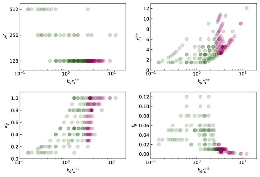
Figure 4: Parameters of 195 individual simulations used in this work. The four-dimensional parameter space is projected on the directions corresponding to the box size ${\cal N}$, the soliton half-peak radius $r_{s}^{\rm init}$, and the parameters of the Maxwell distribution of axion gas $k_{g}$, $f_{g}$. The horizontal axis is common to all panels and shows the product $k_{g}r_{s}^{\rm init}$. Green circles correspond to simulations leading to soliton growth, while red circles show the cases of soliton evaporation. Darker circles indicate multiple realizations of axion gas by changing the phases in the wavefunction.

Our simulations have four input parameters: ${\cal N}$, $k_{g}$, $f_{g}$, and $r_{s}^{\rm init}$, which describe the box size, the momentum distribution of axion gas, and the size of soliton. In this work, we use three box sizes, ${\cal N}=128$, $256$, and $512$. For the regime of light soliton, most of the simulations are conducted with ${\cal N}=128$, while for heavy solitons we use large boxes ${\cal N}=512$ in order to reach low $(k_{g}r_{s})\sim 0.1$. The remaining three parameters are sampled in the ranges

$$k_{g}\in(0.1\,,\,1)~{},~{}~{}~{}~{}~{}f_{g}\in(10^{-4}\,,\,0.12)~{},~{}~{}~{}~{}~{}r_{s}^{\rm init}\in(1.5\,,\,12)\;.$$ (4.10)

Their choice is dictated by the goal to efficiently capture the soliton growth/evaporation within realistic simulation time, while resolving the axion gas and the soliton on the lattice. In addition, they are subject to constraints discussed above which we summarize here for clarity:

• $f_{g}\,k_{g}<0.054\,\left({\cal N}/128\right)^{-2}$: the axion gas does not form a halo due to Jeans instability;

• $r_{s}^{\rm init}<0.1\,{\cal N}$: the effect of periodic images on the soliton is suppressed;

• $\rho_{s,\,{\rm peak}}>30\rho_{g}$: soliton is prominent enough to suppress bias in its mass measurement;

• $M_{s}<0.5\,M_{g}$: soliton does not overwhelm axion waves.

Note that the conditions (a,b) are imposed on the initial configuration, whereas the conditions (c,d) are monitored throughout the whole duration of the simulations. In total we have run 195 simulations with independent realizations of random gas phases. Their parameters are shown in fig. 4 against the product $k_{g}r_{s}^{\rm init}$ which controls the physics of the soliton-gas interaction.

4.2 Growing and evaporating solitons

In this section we present a case study of several simulations that illustrate possible evolution of the soliton-gas system. We use these examples to introduce our procedure for extraction of the soliton growth rate. We also provide evidence that the gas distribution remains close to Maxwellian during the simulations.

We consider three simulation runs with the same initial gas configuration characterized by $({\cal N}=128,k_{g}=1,f_{g}=0.01)$ and different initial soliton sizes $r_{s}^{\rm init}$: $1.51$ (heavy soliton), $2.71$ (median soliton), and $3.62$ (light soliton). Figures 5-7 show the evolution of the soliton characteristics in the three runs. These include the soliton peak density $\rho_{s,\,{\rm peak}}(t)$ (which we identify with the maximal density in the box), the soliton mass $M_{s}(t)$ and the soliton radius $r_{s}(t)$. The peak density is normalized to the mean density of the gas, whereas the mass and radius are determined using the relations (4.9). Clearly, the heavy soliton grows and the light soliton evaporates which is consistent with the analysis of section 3. The median soliton remains approximately unchanged indicating that the transition from growth to evaporation occurs at $(k_{g}r_{s})\sim 2.7$. We also plot in figs. 5-7 the change in the total energy of the axion field in the box. For the median and light solitons the energy is conserved with high precision $|E(t)/E(0)-1|\lesssim 10^{-5}$ throughout the whole duration of the simulations. For the heavy soliton, the energy exhibits a slow drift and the error exceeds $0.1\%$ by the end of the simulations. We associate this with the loss of spatial and temporal resolution for heavy solitons which have small sizes $r_{s}\sim 1$ and high oscillation frequencies $|\mathcal{E}_{s}|\sim 1$ (see section C.1 for a detailed discussion). In our analysis we use only the portion of the simulation where $|E(t)/E(0)-1|<10^{-3}$.

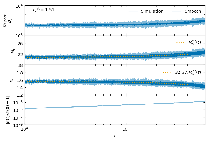
Figure 5: Evolution of the soliton peak density, mass and radius for the case of heavy soliton ($r_{s}^{\rm init}=1.51$). The mass and radius are estimated from the peak density. Thin blue curves show the instantaneous values, whereas the thick curves are obtained by smoothing with a top-hat filter. Yellow dots show the result of fitting the soliton mass with a quadratic polynomial. We also show the time dependence of the total energy in the simulation box used to control the precision of numerical calculations. The gas parameters are (${\cal N}=128$, $k_{g}=1$, $f_{g}=0.01$).

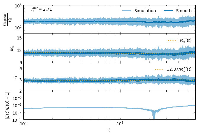
Figure 6: Same as fig. 5 for the case of median soliton ($r_{s}^{\rm init}=2.71$).

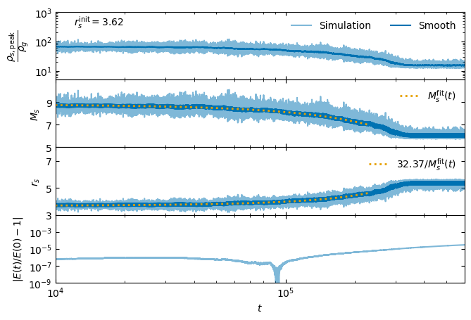
Figure 7: Same as fig. 5 for the case of light soliton ($r_{s}^{\rm init}=3.62$).

We now describe our algorithm to extract the soliton growth rate $\Gamma_{s}$. The task is complicated by strong oscillations of the soliton peak density which are clearly visible in the plots and translate into oscillations of the estimated soliton mass and radius. Such oscillations have been observed in previous works [33, 42] and correspond to the normal modes of the soliton [63, 66] with the frequency of the lowest mode $\omega\sim 0.5\,r_{s}^{-2}$. To mitigate their effect, we construct running averages of the soliton parameters by smoothing them with a top-hat function. We take the width of the top-hat as a function of the initial soliton size $t_{\rm width}=70(r_{s}^{\rm init})^{2}$ which covers about five periods of the oscillations. The resulting smoothed dependences are shown in figs. 5-7 by thick curves.

While smoothing suppresses most of the chaotic oscillations, it still leaves some irregularities in the time dependence of the soliton mass that introduce significant noise when calculating its time derivative. To further suppress this noise, we fit the smoothed mass with an analytic function of time. We have found that a quadratic fit is sufficient in all cases. Thus, we write

$$M_{s}^{\rm fit}(t)=a_{0}+a_{1}t+a_{2}t^{2}\;,$$ (4.11)

where $a_{0}$, $a_{1}$ and $a_{2}$ are fitting parameters. The fitting time-range is determined by the following criteria:

• Inside the range the soliton peak density, mass and radius satisfy the conditions (c,d) from section 4.1;

• The total energy in the simulation box is conserved within precision $|E(t)/E(0)-1|<0.1\%$;

• The time duration is smaller than half of the relaxation time (2.19) to avoid possible changes in the gas distribution due to kinetic relaxation [39].

The best-fit values of $a_{0},a_{1},a_{2}$ for the three sample runs are given in table 1. The corresponding fitted curves are shown in figs. 5-7 with yellow dots. We also define the “fitted” soliton radius by converting it from the soliton mass in accordance with eqs. (4.9),

$$r_{s}^{\rm fit}(t)\equiv\frac{32.37}{M_{s}^{\rm fit}(t)}=\frac{32.37}{a_{0}+a_{1}t+a_{2}t^{2}}\;.$$ (4.12)

The result matches very well the smoothed dependence $r_{s}(t)$, see figs. 5-7. We have verified that an independent fit of smoothed $r_{s}(t)$ with a quadratic polynomial produces essentially identical curves, which provides a consistency check of our procedure.

	$r_{s}^{\rm init}$	$a_{0}$	$a_{1}$	$a_{2}$
heavy soliton	1.51	$20.79$	$0.283\times 10^{-5}$	$0.00239\times 10^{-10}$
median soliton	2.71	$11.35$	$-0.203\times 10^{-5}$	$0.0282\times 10^{-10}$
light soliton	3.62	$8.80$	$-0.595\times 10^{-5}$	$-0.0837\times 10^{-10}$

Table 1: Parameters of the soliton mass fit for the three simulations shown in figs. 5-7. The initial size of the soliton is $r_{s}^{\rm init}$. The parameters of axion gas are ${\cal N}=128$, $k_{g}=1$, $f_{g}=0.01$.

We can now estimate the soliton growth rate substituting the fitted time dependence of the soliton mass in the defining formula (1.3), which yields,

$$\Gamma_{s}^{\rm fit}(t)=\frac{a_{1}+2\,a_{2}\,t}{a_{0}+a_{1}\,t+a_{2}\,t^{2}}\;.$$ (4.13)

We are interested in the dependence of the growth rate on the soliton radius $r_{s}$. Both these quantities depend on time, so a single run provides a continuous set of data points $\big{(}r_{s}^{\rm fit}(t),\Gamma_{s}^{\rm fit}(t)\big{)}$ sampled at different moments of time. In view of uncertainties of our smoothing and fitting procedure, we reduce this set to 20 data points $\big{(}r_{s}^{\rm fit}(t_{i}),\Gamma_{s}^{\rm fit}(t_{i})\big{)}$, $i=1,\ldots,20$, evenly distributed in time within the range of the fitting function $M_{s}^{\rm fit}(t)$. These 20 data points represent the output of a single run. In the next subsection we combine the outputs of 195 runs to build the cumulative dependence of the growth rate on the soliton and gas parameters.

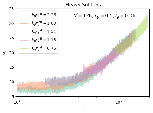
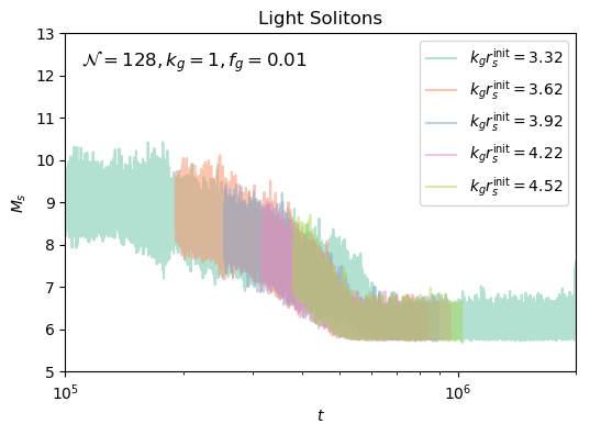
Figure 8: Soliton mass evolution in simulations with $k_{g}r_{s}^{\rm init}$ from 0.75 to 2.26 (top) and from 3.32 to 4.52 (bottom). By shifting the curves along the time axis we have observed that they can be stacked on top of each other.

Soliton growth rate depends on the gas distribution which can, in principle, change during the simulations. This could lead to incompatibility of the results read out at different moments from the start of the runs. To verify that this is not the case, we compare the runs that differ by the initial soliton mass, but have overlapping soliton mass ranges spanned during the evolution. The top panel of fig. 8 shows the evolution of the soliton mass in five simulations of heavy solitons with $k_{g}r_{s}^{\rm init}$ varying from $0.75$ to $2.26$. The gas parameters are chosen the same in all five runs $({\cal N}=128,\,k_{g}=0.5,\,f_{g}=0.06)$. The curves have been shifted in time until they overlap. We observe that the curves are well aligned with each other. In the lower panel of fig. 8 we repeat the same exercise for five light soliton simulations with $k_{g}r_{s}^{\rm init}$ from $3.32$ to $4.52$ and the gas parameters $({\cal N}=128,\,k_{g}=1,\,f_{g}=0.01)$. The stacked curves are again well aligned. We conclude that the soliton growth rate depends only on the initial gas parameters and the instantaneous soliton mass (or radius), and is insensitive to the previous evolution of the soliton-gas system. This justifies combination of the results extracted from different runs at different stages of simulations.

The above results suggest that the gas distribution remains close to Maxwellian during the simulations with solitons. We have measured the distribution directly at different moments of time and have seen that it is compatible with Maxwellian, though the measurement is rather noisy, see fig. 16 in appendix B. This is in stark contrast with simulations [39] without initial soliton where the gas distribution exhibits distinct evolution on the time scale $\tau_{\rm rel}$ (eq. 2.19) towards populating low-momentum modes which culminates in the soliton formation. However, as discussed in appendix B, the distribution appears to return to Maxwellian after the soliton is formed. We also find that the growth of the soliton mass, though faster than in the Maxwellian gas right after the formation, approaches the Maxwellian rate within time of order $\tau_{\rm rel}$, see fig. 15. This gives another evidence that the presence of the soliton “Maxwellizes” the gas.

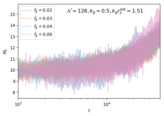
Figure 9: Growth of the soliton mass in the simulations with the same values of $({\cal N}=128,\,k_{g}=0.5,\,k_{g}r_{s}^{\rm init}=1.51)$ and varying $f_{g}$. The time axis in different runs has been scaled by $f_{g}^{2}$ and normalized to the case $f_{g}=0.06$. The time span of the curves is restricted to half of the relaxation time (2.19) and covers the portion of the data used in the measurement of the soliton growth rate.

The analytic derivation of section 3 implies that at fixed $k_{g}r_{s}$ the soliton growth/evaporation rate is proportional to $\rho_{g}^{2}/k_{g}^{6}\propto f_{g}^{2}$. To verify if this scaling holds in the simulations, we perform several runs with the same ${\cal N}$, $k_{g}$ and $r_{s}^{\rm init}$, but different $f_{g}$. We measure the time dependence of the soliton mass and scale the time axis by $f_{g}^{2}$. The results are shown in fig. 9. We see a satisfactory agreement between different curves. A slightly faster growth of the curve with the highest value of $f_{g}$ at late times can be due to the fact that the gas in this case is closer to the Jeans instability leading to the development of an overdensity (proto-halo) around the soliton. We have clearly seen this overdensity in the runs with the parameters near the Jeans instability limit (4.7) and observed that it is correlated with the increase of the ratio $\Gamma_{s}/f_{g}^{2}$. The associated bias is comparable to the other uncertainties in the measurement of $\Gamma_{s}$ and is included in the error bars for our final results in the next section.

4.3 Results

In this section, we construct the cumulative dependence of $\Gamma_{s}$ on the soliton and gas parameters. As explained above, each simulation run produces 20 data points $(r_{s},\Gamma_{s})$. We collect the data points from 195 runs and bin them in logarithmic scale in $k_{g}r_{s}$. In each bin we compute the average value and variance of

$$\Gamma_{s}\times\frac{(4\pi)^{3}}{f_{g}^{2}}=\Gamma_{s}\times\frac{k_{g}^{6}}{\rho_{g}^{2}}\;.$$ (4.14)

The results of this procedure are shown in fig. 10. Note that we restore the dimensionful constants in the scale of $\Gamma_{s}$ in the figure.

Consistently with the analysis of section 3, the growth rate is positive at small $k_{g}r_{s}$ (heavy solitons) corresponding to the soliton growth, and is negative at large $k_{g}r_{s}$ (light solitons) corresponding to evaporation. Moreover, the data points with the largest values of $k_{g}r_{s}$ match the asymptotic dependence (3.23), including the numerical coefficient (3.24),

$$\Gamma_{s}\simeq-2.6\times\frac{(4\pi G)^{2}m^{3}\rho_{g}^{2}}{k_{g}^{6}}\,(k_{g}r_{s})^{2}\;.$$ (4.15)

This dependence is shown by the blue line. Thus, we conclude that the asymptotics (3.23) are reached already at $k_{g}r_{s}\gtrsim 5$. The transition from evaporation to growth happens at $k_{g}r_{s}\sim 2.5$ which is in reasonable agreement with the naive estimate (3.25). In terms of the gas and soliton virial temperatures, it corresponds to $T_{g}/T_{s}\simeq 12$.

For lower $k_{g}r_{s}$ the soliton grows. The growth rate stays almost constant in the range $0.7<k_{g}r_{s}<2$ where it is comparable to the inverse of the gas relaxation time $\tau_{\rm rel}^{-1}$, see eq. 2.19. The lower end of the plateau corresponds to the equality of the gas and soliton virial temperatures, $T_{g}/T_{s}=1$, which is marked by the dashed vertical line in fig. 10.

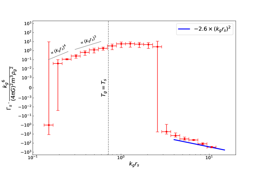
Figure 10: The soliton growth/evaporation rate as function of $k_{g}r_{s}$ — the product of the gas momentum and the soliton half-density radius. The cumulative dependence is constructed using 3900 data points extracted from 195 independent simulations with different gas and soliton parameters. The data are binned on logarithmic scale in $k_{g}r_{s}$. Each dot gives the average value of the growth rate in the bin, while the vertical error bars correspond to the standard deviation within the bin. The blue solid line shows the asymptotic dependence predicted by eq. 3.23. At small $k_{g}r_{s}$ the dotted lines indicate possible power-law dependences. The dashed vertical line marks the value of $k_{g}r_{s}$ corresponding to the equality of the gas and soliton virial temperatures, $T_{g}/T_{s}=1$.

At $k_{g}r_{s}<0.7$ (equivalently $T_{g}/T_{s}<1$) the growth rate quickly decreases. We find that this decrease is consistent with a power law

$$\Gamma_{s}\propto(k_{g}r_{s})^{n}$$ (4.16)

with $n\simeq 3$ indicated by the dotted line in the plot. The points with the smallest values of $k_{g}r_{s}$ hint at a steepening dependence with $n=4$ at $k_{g}r_{s}\to 0$, in agreement with the analytic estimate (3.31). There are, however, several caveats that prevent us from claiming that we have reached the heavy soliton asymptotics. First, as pointed out in section 3.3, the expression (3.31) has been obtained under the assumption that the contribution of the bound states into the soliton growth scales with $k_{g}r_{s}$ in the same way as the contribution of states from continuum. This assumption must be verified by analyzing the kinetic cascade in the soliton–gas system which is beyond the scope of the present paper. Second, the low-$(k_{g}r_{s})$ bins in our simulations are at the extreme of the numerical resolution and close to the threshold for halo formation. Therefore they can be affected by systematics. Without the three lowest-$(k_{g}r_{s})$ bins the numerical data are compatible with a shallower slope $n=2$. All in all, the heavy soliton limit is challenging both to numerical and analytical methods. Taking into account the uncertainties, we conservatively conclude that the power $n$ in eq. 4.16 for heavy solitons lies in the range $2\leq n\leq 4$. More work is needed to pin down the precise asymptotic value of $n$ at $k_{g}r_{s}\to 0$.

5 Discussion and outlook

Absence of kinetic equilibruium.

We have found that a soliton (boson star) immersed into a homogeneous Maxwellian axion gas evaporates if its virial temperature is about 12 times lower than the virial temperature of the gas, and grows otherwise. This rules out the possibility of a stable kinetic equilibrium between the gas and the soliton.

Evaporation of light solitons.

Though evaporation of cold solitons may at first sight appear surprising, the mechanism behind it is quite intuitive. Being a self-gravitating system, the soliton possesses negative heat capacity. Thus, a transfer of energy from the hot gas to the cold soliton makes the latter even colder. This leads to a run-away of the soliton temperature, and hence its mass, towards zero.

The parametric dependence of the evaporation rate can be estimated using the following simple considerations. Wave interference in the axion gas produces density inhomogeneities with the characteristic size of half de Broglie wavelength $\lambda_{a}/2=\pi/k_{g}$. These inhomogeneities can be though of as quasi-particles with the mass $M_{qp}\sim\rho_{g}(\lambda_{a}/2)^{3}$ [12]. A single quasi-particle colliding with the soliton transfers to it a recoil momentum

$$\delta p\sim\frac{GM_{s}M_{qp}}{r_{s}^{2}}\cdot\frac{r_{s}}{v_{qp}}\;,$$ (5.1)

where $v_{qp}\sim k_{g}/m$ is the quasi-particle velocity, and $r_{s}$ appears as the typical impact parameter. This implies the soliton recoil energy

$$\delta E_{s}\sim\frac{\delta p^{2}}{2M_{s}}\sim\frac{G^{2}M_{qp}^{2}M_{s}}{2r_{s}^{2}v_{qp}^{2}}\;.$$ (5.2)

Since the size of the quasi-particle is smaller than $r_{s}$ for the light soliton, the recoil energy is distributed non-uniformly throughout the soliton volume. This leads to excitation of its normal modes. The number of axions that get excited from the ground state and hence get lost by the soliton is of order $\delta N_{s}\sim-\delta E_{s}/|\mathcal{E}_{s}|$. Combining everything together, we obtain the mass loss of the soliton in a single quasi-particle collision,

$$\frac{\delta M_{s}}{M_{s}}\sim-\frac{G^{2}M_{qp}^{2}m^{2}}{2v_{qp}^{2}}\;,$$ (5.3)

where we have used that $|\mathcal{E}_{s}|r_{s}^{2}\sim 1/m$. To obtain the evaporation rate, we have to multiply this result by the number of quasi-particles bombarding the soliton in a unit of time, $J_{qp}\sim 4\pi r_{s}^{2}(\lambda_{a}/2)^{-3}v_{qp}$. In this way we arrive at

$$\Gamma_{s}\sim-\frac{2\pi^{4}G^{2}m^{3}\rho_{g}^{2}}{k_{g}^{6}}\,(k_{g}r_{s})^{2}\;,$$ (5.4)

which agrees with the exact expression (4.15) obtained from the kinetic theory, up to a factor about $0.5$.

We have seen that the threshold for evaporation is set by the equality of the evaporation rate and the relaxation rate in the gas — a competing process leading to the soliton formation [39]. This explains why the solitons that are formed in the gas always have virial temperature comparable to that of the gas: they are just hot (and heavy) enough to survive.

In what physical situation can the soliton evaporation be relevant? For fuzzy dark matter, this is the case when a small subhalo with low velocity dispersion and light solitonic core falls into a bigger halo with higher velocity dispersion. Evaporation then adds a new destruction mechanism for the subhalo soliton, on top of the tidal stripping [60]. The time scale of evaporation is given by the inverse of $|\Gamma_{s}|$,

$$t_{\rm evap}\simeq 2.4\times 10^{9}\,\left(\frac{m}{10^{-21}\,{\rm eV}}\right)^{3}\,\left(\frac{\rho_{g}}{{0.3\,{\rm GeV/cm^{3}}}}\right)^{-2}\,\left(\frac{v_{g}}{30\,{\rm km/s}}\right)^{6}\,\left(\frac{k_{g}r_{s}}{10}\right)^{-2}{\rm yr}\;,$$ (5.5)

where $\rho_{g}$ and $v_{g}$ should be taken as the density and velocity dispersion of the bigger halo at the orbit of the soliton. The evaporation time is very sensitive to the halo parameters and can be longer or shorter than the age of the universe depending on their precise values. The evaporation should be also taken into account in the evolution of boson stars in merging QCD axion miniclusters. Though here the particle mass is much higher, the evaporation time can still be much shorter than the age of the universe due to the very small velocity dispersion $v_{g}\sim 10^{-5}\,{\rm km/s}$ in the miniclusters and their extremely high density $\rho_{g}\gtrsim 10^{6}\,{\rm GeV/cm^{3}}$ [67].

Growth of heavy solitons.

For solitons with virial temperature above the evaporation threshold ($T_{s}\gtrsim 0.1\,T_{g}$) we have found that the growth rate quickly decreases once the soliton temperature exceeds that of the gas. This result is in qualitative agreement with other works [39, 48]. The growth rate of heavy solitons measured from our numerical simulations is consistent with the power law (4.16) with $n$ between $2$ and $4$. We have presented analytic arguments favoring $n=4$ in the limit $k_{g}r_{s}\to 0$, which is compatible with the numerical data in the lowest $k_{g}r_{s}$ bins. These bins, however, suffer from large uncertainties and it remains unclear if the range $k_{g}r_{s}\gtrsim 0.2$ probed in the simulations is sufficient to reach into the asymptotic heavy soliton regime.

The power-law dependence of the rate (4.16) translates into power-law growth of the soliton mass,

$$M_{s}\propto t^{\alpha}\;,~{}~{}~{}~{}~{}~{}\alpha=1/n\;.$$ (5.6)

Ref. [39] established that $\alpha=1/2$ provides a good fit to the soliton growth right after formation, whereas Ref. [48] found a dramatic flattening of the soliton mass curve at late times corresponding to $\alpha=1/8$. The results of Ref. [39] are consistent with ours, though our central value for the power $n=3$ predicts a somewhat shallower dependence with $\alpha=1/3$. The steep growth observed in [39] might be due to a short duration of the simulations. Indeed, by carrying out numerical experiments with the same setup as in [39] (see appendix B) and fitting the soliton mass with the formula (5.6), we have observed a correlation of the best-fit index $\alpha$ with the soliton lifetime: $\alpha$ is about $1/2$ for newly formed solitons and descreases down to $1/4$ for grown-up solitons long after the relaxation time (see fig. 14). This trend is in agreement with our main simulations where we see indications of increasing $n$, and hence decreasing $\alpha$, for heavier solitons. However, at this point the numerical data are rather inconclusive as to the robustness of this trend and the asymptotic value of $\alpha$ at $t\to\infty$.

On the other hand, we do not see any evidence for the low $\alpha=1/8$ found in [48]. Moreover, our analytic considerations suggest that the asymptotic value of $\alpha$ is at least as high as $1/4$. The discrepancy may be due to the difference in the setups. We study a soliton in a homogeneous gas, whereas Ref. [48] considers a soliton in the center of an axion halo. It is conceivable that suppression of the soliton growth in the latter case stems from its back reaction on the halo. It will be interesting to explore this possibility in more detail in future.

Soliton-host halo relation.

One can ask whether our results have any implications for the soliton-host halo relation. The answer is: Not directly, because in the cosmological setting the solitons were found to form during the initial halo collapse when axions are not yet in the kinetic regime. Still, with some degree of extrapolation, one can argue that our results make unlikely formation of a light soliton since it would be evaporated by the fast axions from the halo. This sets a lower bound on the soliton mass which is just a factor of a few lower than $M_{s}^{\rm SSH}$, the mass corresponding to the soliton-host halo relation. Heavier solitons can, in principle, form with arbitrary masses and will continue growing upon the halo virialization. The time scale for this growth can, however, be very long and exceed the age of the universe when the soliton mass exceeds $M_{s}^{\rm SSH}$. Moreover, it is natural to speculate that the solitons are more likely to form as light as they can which singles out $M_{s}^{\rm SSH}$ as the sweet spot. This reasoning still does not tell us how far the soliton-host halo relation can be extrapolated in the parameter space. In particular, we do not know whether the solitons form in any halo and for any value of axion mass, or for some parameters their formation becomes improbable. More work is needed to answer these questions.

Persistence of Maxwell distribution.

It is known that without a soliton the velocity distribution of axion gas relaxes towards thermal form with high population of low-momentum modes [39]. We have found evidence that the presence of soliton changes the picture. In this case the Maxwell distribution appears to persist on timescales significantly longer than the kinetic relaxation time. Moreover, in the simulations with soliton formation we observed restoration of the Maxwell distribution after a transient period with enhanced population of low-momentum modes preceding the birth of the soliton. This “Maxwellization” manifests itself indirectly in the universality of the soliton mass evolution in simulations with different histories (figs. 8, 15), as well as in the directly measured momentum distribution at different moments of time (fig. 16). The latter, however, is subject to large temporal fluctuations which presently do not allow us to move beyond qualitative statements. It will be interesting to study this phenomenon more quantitatively in future by developing methods of measuring the momentum distribution with reduced noise. A complementary approach would be to track the distribution of axions in energy, instead of momentum, as suggested in Ref. [39].

Appendix A Classical derivation of the soliton growth rate

In this appendix we derive the expression (3.9) for the soliton growth rate as the consequence of the classical equations of motion. It is convenient to integrate out the gravitational potential and rewrite the Schrödinger–Poisson system as a single equation with non-local interaction,

$$i\partial_{t}\psi+\frac{\Delta\psi}{2m}-4\pi Gm^{2}\psi\frac{1}{\Delta}|\psi|^{2}=0\;,$$ (A.1)

where $\tfrac{1}{\Delta}$ denotes the Green’s function of the Laplacian. Clearly, this equation conserves the total mass of axions in a box $M_{\rm tot}=m\int d^{3}x|\psi|^{2}$. Now, we make the split (2.22) into the soliton and gas and, using the fact that the soliton is a solution of eq. A.1, obtain the equation for the gas component,

$$\begin{split}i\partial_{t}\psi_{g}+\frac{\Delta\psi_{g}}{2m}&-4\pi Gm^{2}\bigg{[}\psi_{g}\frac{1}{\Delta}|\psi_{s}|^{2}+\psi_{s}\frac{1}{\Delta}(\psi_{s}^{*}\psi_{g})+\psi_{s}\frac{1}{\Delta}(\psi_{s}\psi_{g}^{*})\bigg{]}\\ &-4\pi Gm^{2}\bigg{[}\psi_{g}\frac{1}{\Delta}(\psi_{s}^{*}\psi_{g})+\psi_{g}\frac{1}{\Delta}(\psi_{s}\psi_{g}^{*})+\psi_{s}\frac{1}{\Delta}|\psi_{g}|^{2}+\psi_{g}\frac{1}{\Delta}|\psi_{g}|^{2}\bigg{]}=0\;.\end{split}$$ (A.2)

In the first line we have grouped the terms that affect the gas field at linear order, whereas the second line contains interactions. Note that, despite the presence of the small factor $4\pi Gm^{2}$, all terms in the first line are of the same order because $\psi_{s}$ is proportional to $(4\pi Gm^{2})^{-1/2}$, see eq. 2.4. Correspondingly, the leading interaction terms are of order $\sqrt{4\pi Gm^{2}}$.

The mass of the gas is not constant. From eq. A.2 we have,

$$\frac{dM_{g}}{dt}=m\frac{d}{dt}\int d^{3}x|\psi_{g}|^{2}=-(8\pi Gm^{3})\mathop{\rm Im}\nolimits\int d^{3}x\bigg{[}\psi_{s}^{*}\psi_{g}\frac{1}{\Delta}(\psi_{s}^{*}\psi_{g})+\psi_{s}^{*}\psi_{g}\frac{1}{\Delta}|\psi_{g}|^{2}\bigg{]}\;,$$ (A.3)

where we have canceled the boundary terms assuming periodic boundary conditions. Since the total mass is conserved, this must be compensated by the change in the soliton mass. Thus, we obtain for the soliton growth rate,

$$\Gamma_{s}=\frac{8\pi Gm^{3}}{M_{s}}\mathop{\rm Im}\nolimits\int d^{3}x\bigg{[}\psi_{s}^{*}\psi_{g}\frac{1}{\Delta}(\psi_{s}^{*}\psi_{g})+\psi_{s}^{*}\psi_{g}\frac{1}{\Delta}|\psi_{g}|^{2}\bigg{]}\;.$$ (A.4)

If we neglect the interaction terms in eq. A.2, it admits a set of periodic-in-time solutions. We decompose the gas field in these eigenmodes,

$$\psi_{g}(t,\mathbf{x})=\sum_{i}a_{i}(t){\rm e}^{-i\mathcal{E}_{i}t}\psi_{i}(\mathbf{x})\;,$$ (A.5)

where the amplitudes $a_{i}(t)$ slowly vary due to the interactions. Substituting into eq. A.4 we obtain,

$$\Gamma_{s}=-\frac{2m}{M_{s}}\mathop{\rm Im}\nolimits\bigg{[}\sum_{i,j}a_{i}a_{j}{\rm e}^{-i(\mathcal{E}_{i}+\mathcal{E}_{j}-2\mathcal{E}_{s})t}A^{\prime}_{is,js}+\sum_{i,j,k}a_{i}a_{j}a_{k}^{*}{\rm e}^{-i(\mathcal{E}_{i}+\mathcal{E}_{j}-\mathcal{E}_{k}-\mathcal{E}_{s})t}A^{\prime}_{is,jk}\bigg{]}\;,$$ (A.6)

where the scattering amplitude $A^{\prime}_{is,jk}$ is defined in eq. 3.8, and $A^{\prime}_{is,js}$ is defined similarly with the $k$th wavefunction replaced by the soliton. All terms in the first sum quickly oscillate since the gas states are separated from the ground state by an energy gap of order $|\mathcal{E}_{s}|$. Thus, they disappear once we average the growth rate over time scales of order $|\mathcal{E}_{s}|^{-1}$ and we omit them in what follows.

The second sum does not vanish upon time averaging because the combination of energies in the exponent can be small. However, to obtain the physical growth rate we also have to average over random initial phases of the gas amplitudes. In the absence of interactions the amplitudes $a_{i}$ in eq. A.6 coincide with the initial amplitudes $a_{i}^{(0)}$ and thus averaging over their phases will give $\Gamma_{s}=0$. To obtain a non-zero result, we have to take into account gas interactions.

The first correction to the free gas field is due to terms of order $\sqrt{4\pi Gm^{2}}$ in eq. A.2. We can write it schematically as

$$\psi_{g}^{(1)}=(4\pi Gm^{2})\,{\cal G}_{\rm ret}*\bigg{\{}\psi_{g}^{(0)}\frac{1}{\Delta}\big{(}\psi_{s}^{*}\psi_{g}^{(0)}\big{)}+\psi_{g}^{(0)}\frac{1}{\Delta}\big{(}\psi_{s}{\psi_{g}^{(0)}}^{*}\big{)}+\psi_{s}\frac{1}{\Delta}|\psi_{g}^{(0)}|^{2}\bigg{\}}\;,$$ (A.7)

where $\psi_{g}^{(0)}$ is the free gas field and ${\cal G}_{\rm ret}$ is the retarded Green’s function of the operator in the first line of (A.2). Using the complete set of eigenmodes, it can be written as,

$${\cal G}_{\rm ret}(t-t^{\prime},\mathbf{x},\mathbf{x}^{\prime})=\sum_{i}\int\frac{d\mathcal{E}}{2\pi}\,\frac{\psi_{i}(\mathbf{x})\psi_{i}^{*}(\mathbf{x}^{\prime})}{\mathcal{E}-\mathcal{E}_{i}+i\epsilon}\,{\rm e}^{-i\mathcal{E}(t-t^{\prime})}\;.$$ (A.8)

Substituting this expression into (A.7) and expanding $\psi_{g}^{(1)}$ and $\psi_{g}^{(0)}$ into eigenmodes, we obtain the first-order correction to the amplitudes,

$$\begin{split}a_{i}^{(1)}=-\sum_{j,k}\bigg{[}&a_{j}^{(0)}a_{k}^{(0)}\frac{{\rm e}^{-i(\mathcal{E}_{j}+\mathcal{E}_{k}-\mathcal{E}_{i}-\mathcal{E}_{s})t}}{\mathcal{E}_{j}+\mathcal{E}_{k}-\mathcal{E}_{i}-\mathcal{E}_{s}+i\epsilon}A^{\prime}_{ks,ji}\\ &+a_{j}^{(0)}{a_{k}^{(0)}}^{*}\frac{{\rm e}^{-i(\mathcal{E}_{j}-\mathcal{E}_{k}-\mathcal{E}_{i}+\mathcal{E}_{s})t}}{\mathcal{E}_{j}-\mathcal{E}_{k}-\mathcal{E}_{i}+\mathcal{E}_{s}+i\epsilon}(A^{\prime*}_{ks,ij}+A^{\prime*}_{is,kj})\bigg{]}\;.\end{split}$$ (A.9)

Next, we insert this expression into the first-order contribution to the soliton growth rate,

$$\Gamma_{s}^{(1)}=-\frac{2m}{M_{s}}\sum_{i,j,k}\Big{(}a_{i}^{(1)}a_{j}^{(0)}{a_{k}^{(0)}}^{*}+a_{i}^{(0)}a_{j}^{(1)}{a_{k}^{(0)}}^{*}+a_{i}^{(0)}a_{j}^{(0)}{a_{k}^{(1)}}^{*}\Big{)}{\rm e}^{-i(\mathcal{E}_{i}+\mathcal{E}_{j}-\mathcal{E}_{k}-\mathcal{E}_{s})t}A^{\prime}_{is,jk}\;,$$ (A.10)

and average over the phases of $a_{i}^{(0)}$ using

$$\langle a_{i}^{(0)}a_{j}^{(0)}{a_{i^{\prime}}^{(0)}}^{*}{a_{j^{\prime}}^{(0)}}^{*}\rangle=f_{i}f_{j}(\delta_{ii^{\prime}}\delta_{jj^{\prime}}+\delta_{ij^{\prime}}\delta_{ji^{\prime}})\;.$$ (A.11)

Upon a somewhat lengthy, but straightforward calculation, we arrive at

$$\begin{split}\langle\Gamma_{s}\rangle=\frac{m}{M_{s}}\mathop{\rm Im}\nolimits\sum_{i,j,k}\bigg{\{}&\frac{f_{j}f_{k}+f_{i}f_{k}}{\mathcal{E}_{k}-\mathcal{E}_{j}-\mathcal{E}_{i}+\mathcal{E}_{s}+i\epsilon}|A^{\prime}_{is,jk}+A^{\prime}_{js,ik}|^{2}\\ &+\frac{f_{j}f_{k}}{-\mathcal{E}_{i}+\mathcal{E}_{s}+i\epsilon}\Big{[}(A^{\prime}_{is,jj}+A^{\prime}_{js,ij})(A^{\prime*}_{is,kk}+A^{\prime*}_{ks,ik})+{\rm h.c.}\Big{]}\\ &+\frac{f_{i}f_{j}}{\mathcal{E}_{i}+\mathcal{E}_{j}-\mathcal{E}_{k}-\mathcal{E}_{s}-i\epsilon}|A^{\prime}_{is,jk}+A^{\prime}_{js,ik}|^{2}\bigg{\}}.\end{split}$$ (A.12)

In the final step we use the formula

$$\mathop{\rm Im}\nolimits\frac{1}{z+i\epsilon}=-i\pi\delta(z)\;.$$ (A.13)

Then the second term vanishes because $\mathcal{E}_{i}\neq\mathcal{E}_{s}$, whereas the rest of the terms reproduce eq. 3.9. Thus, we have shown that the classical derivation leads to the same soliton growth rate as the quantum mechanical one, upon averaging over the ensemble of gas realizations with different initial phases.

The above derivation also allows us to estimate the r.m.s. fluctuations of $\Gamma_{s}$ in individual realizations. To this aim, let us return to eq. A.6 and smooth it with a Gaussian filter over time scales $\langle\Gamma_{s}\rangle^{-1}>\tau\gg|\mathcal{E}_{s}|^{-1}$. We obtain,

$$\Gamma_{s}=-\frac{2m}{M_{s}}\mathop{\rm Im}\nolimits\sum_{i,j,k}a_{i}a_{j}a_{k}^{*}{\rm e}^{-i(\mathcal{E}_{i}+\mathcal{E}_{j}-\mathcal{E}_{k}-\mathcal{E}_{s})t}A^{\prime}_{is,jk}{\rm e}^{-\tau^{2}(\mathcal{E}_{i}+\mathcal{E}_{j}-\mathcal{E}_{k}-\mathcal{E}_{s})^{2}/2}\;.$$ (A.14)

To get the r.m.s. fluctuations, we subtract $\langle\Gamma_{s}\rangle$, square the result and average over the gas phases. In the latter step we can replace $a_{i}$ with $a_{i}^{(0)}$ to obtain the leading contribution. Retaining only the unsuppressed terms we obtain,

$$\begin{split}\langle\delta\Gamma_{s}^{2}\rangle&\simeq\bigg{(}\frac{m}{M_{s}}\bigg{)}^{2}\sum_{i,j,k}f_{i}f_{j}f_{k}\,|A^{\prime}_{is,jk}+A^{\prime}_{js,ik}|^{2}{\rm e}^{-\tau^{2}(\mathcal{E}_{i}+\mathcal{E}_{j}-\mathcal{E}_{k}-\mathcal{E}_{s})^{2}}\\ &\simeq\frac{\sqrt{\pi}}{\tau}\bigg{(}\frac{m}{M_{s}}\bigg{)}^{2}\sum_{i,j,k}f_{i}f_{j}f_{k}\,|A^{\prime}_{is,jk}+A^{\prime}_{js,ik}|^{2}\delta(\mathcal{E}_{i}+\mathcal{E}_{j}-\mathcal{E}_{k}-\mathcal{E}_{s})\;.\end{split}$$ (A.15)

Comparing this with the expression (3.9) for the rate, we get an estimate

$$\langle\delta\Gamma_{s}^{2}\rangle\sim\frac{1}{\tau}\frac{m}{M_{s}}f_{g}\langle\Gamma_{s}\rangle\;.$$ (A.16)

The fluctuations are much smaller than the average if $\langle\Gamma_{s}\rangle\tau\gg mf_{g}/M_{s}$ which can be always achieved by an appropriate choice of the smoothing scale, as long as the number of particles in the soliton is much larger than the occupation numbers of individual modes in the gas, $M_{s}/m\gg f_{g}$.

Appendix B Formation of axion soliton from the gas

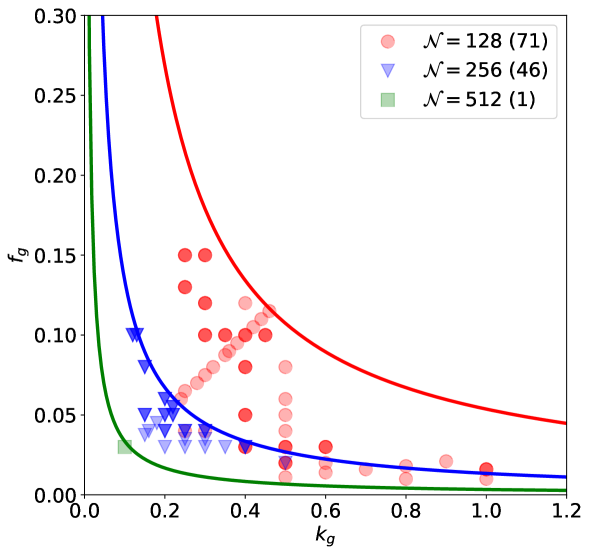
Figure 11: Gas parameters for the simulations with soliton formation. Solid lines bound the regions without Jeans instability for different simulation box sizes (see eq. 4.7). The number of runs on different lattices is indicated in parenthesis.

In this appendix we report the results of simulations with formation of the soliton from the gas. We use the same numerical scheme and initial conditions for the gas as described in section 4.1, but we do not put the initial soliton. Instead, we wait for the soliton to emerge spontaneously. The purpose of these simulations is twofold. First, we cross-check our numerical approach by comparing with the simulations carried out in [39]. Second, we investigate to what extent the evolution of spontaneously formed solitons is similar to the evolution of the solitons inserted into the gas from the start.

We perform 118 independent simulations with the parameters summarized in fig. 11. The parameter space is restricted by the requirement of absence of the Jeans instability, so that the gas does not form a halo and remains homogeneous.

Figure 12 shows the results of a typical simulation run. The maximal axion density within the simulation box remains small for time less than the relaxation time (2.19) marked with the red dotted line. Then it starts growing which signals the formation of a soliton. As in section 4, we determine the soliton mass from its peak density using eq. 4.9. We also construct smoothed peak density and soliton mass using a top-hat filter with the width $t_{\rm width}=70/k_{g}^{2}$. The smoothed dependences are shown in the figure with thick blue lines.

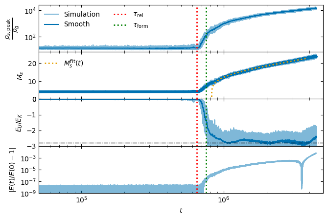
Figure 12: Example of spontaneous soliton formation in axion gas with parameters ${({\cal N}=128,k_{g}=0.5,f_{g}=0.02)}$. From top to bottom: maximal density in the simulation box, soliton mass estimated from the peak density, virial ratio $E_{U}/E_{K}$, total energy in the box. Thick blue lines show the smoothed dependences. Yellow dotted line is the fit (B.2). Vertical red and green dotted lines mark the relaxation time (2.19) and the measured soliton formation time, respectively.

To pin down the moment of soliton formation, we use the method proposed in [33]. We identify the density maximum within the simulation box and compute the kinetic ($E_{K}$) and potential ($E_{U}$) energy in a spherical region around it. The radius of the sphere is chosen as the radius at which the shell-averaged density drops to half of its peak value. To calculate the kinetic energy, we evaluate the field gradient, subtract the center-of-mass velocity contribution, square the result and integrate over the volume of the sphere. The potential energy is approximated by the potential energy of a uniform ball with the mass enclosed inside the sphere. For a random peak in the gas the ratio $E_{U}/E_{K}$ is close to zero, whereas for the soliton it obeys the virial condition $E_{U}/E_{K}\simeq-2.8$. In fig. 12 we see that this ratio changes abruptly from $0$ to $-2.8$ around $t\sim\tau_{\rm rel}$. We identify the soliton formation time $\tau_{\rm form}$ as the moment when the smoothed curve $E_{U}/E_{K}$ crosses half of its virial value,

$$E_{U}/E_{K}\Big{|}_{\tau_{\rm form}}=-1.4\;.$$ (B.1)

This time is marked with the green dotted line in the plot. We see that it agrees well with the relaxation time $\tau_{\rm rel}$.

Ref. [39] suggested that upon formation the growth of the soliton is described by a power-law

$$M_{s}(t)=M_{0}\left(\dfrac{t}{\tau_{0}}-1\right)^{\alpha}$$ (B.2)

with $\alpha=1/2$, $\tau_{0}=\tau_{\rm rel}$ and $M_{0}\simeq 12\pi k_{g}$. To verify if this law is obeyed in our simulations, we fit the smoothed soliton mass at $t>\tau_{\rm form}$ with the formula (B.2) allowing $\alpha$, $\tau_{0}$, $M_{0}$ to vary as free fitting parameters. The fitting time range is restricted by the condition that the energy error $\left|E(t)/E(0)-1\right|$ does not exceed $0.1\%$. The result of the fit is shown by yellow dotted line in fig. 12. The best-fit parameters for this run are $\alpha=0.22$, $\tau_{0}=8.2\times 10^{5}$, $M_{0}=17.03$. Note that the value of $\alpha$ is significantly lower than $1/2$. We will discuss shortly how this result can be reconciled with those of Ref. [39].

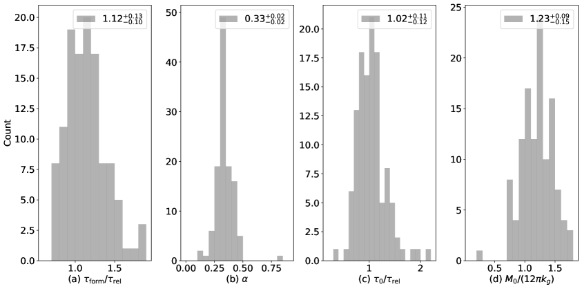
Figure 13: Results of the measurements in the simulations with soliton formation. The histograms show the distributions of the soliton formation time $\tau_{\rm form}$, and the parameters in the power-law fit (B.2) of the soliton mass growth: $\alpha$, $\tau_{0}$, $M_{0}$. The relaxation time $\tau_{\rm rel}$ is given by eq. 2.19 and $k_{g}$ is the gas momentum.

We repeat the above analysis for each of 118 runs and construct the histograms of $\tau_{\rm form}$, $\alpha$, $\tau_{0}$, $M_{0}$ measured in different runs. These histograms are shown in fig. 13 together with their means and standard deviations. The mean values of $\tau_{\rm form}$, $\tau_{0}$ and $M_{0}$ are in good agreement with the findings of [39]. On the other hand, for the exponent we obtain a lower mean, $\alpha=0.33\pm 0.02$. It is important to notice, however, that the distribution of $\alpha$ is quite broad, extending from $0.2$ to $0.5$. From the analysis in the main text we know that the soliton growth rate decreases when the soliton gets heavier. This suggests that the spread in $\alpha$ can arise due to different soliton masses achieved in different simulations. In this picture, the runs with larger duration should yield lower values of $\alpha$ since the solitons in them have more time to grow.

Figure 14: The exponent in the power-law fit (B.2) for the soliton mass against final simulation time $t_{\rm end}$ measured in units of the relaxation time (2.19). Longer simulations produce more massive solitons which have slower growth rate and hence lower values of $\alpha$. Three outlier simulations with $\alpha\simeq 0.8$ and $\alpha\simeq 0.1$ represent large fluctuations of unknown origin.

To check this expectation, we plot in fig. 14 the best-fit value of $\alpha$ as function of the duration of the simulation in units of relaxation time. Apart from a few outliers, the bulk of the data exhibit a pronounced anti-correlation between $\alpha$ and $t_{\rm end}/\tau_{\rm rel}$. The exponent varies from $\alpha\simeq 0.5$ for newly-born solitons down to $\alpha\lesssim 0.25$ for long-lived solitons. Thus, the value $\alpha=1/2$ found in [39] can be explained by short duration of the simulations used in the analysis, whereas longer simulations carried out in the present work uncover a trend for the decrease of $\alpha$ with time. This trend is consistent, both qualitatively and quantitatively, with the results on heavy soliton growth from the main text. Indeed, the scaling (4.16) of the soliton growth rate implies

$$\frac{1}{M_{s}}\frac{dM_{s}}{dt}\propto\frac{1}{M_{s}^{n}}~{}~{}~{}~{}~{}\Longrightarrow~{}~{}~{}~{}~{}M_{s}\propto\bigg{(}\frac{t}{\tau_{0}}-1\bigg{)}^{1/n}\;,$$ (B.3)

which leads to the identification $\alpha=1/n$. Thus, the slow-down of the soliton growth with $\alpha$ decreasing from $1/2$ to $1/4$ as time goes on matches the steepening of the $\Gamma_{s}$ dependence on $k_{g}r_{s}$ with $n$ increasing from $2$ to $4$ at smaller $k_{g}r_{s}$ (see section 4.3).

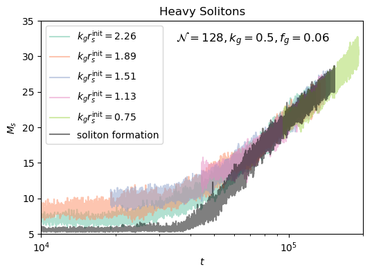
Figure 15: Same as upper panel in fig. 8 with the addition of the soliton mass evolution from a run with soliton formation (in grey). The spontaneously formed soliton approaches the same growth rate as the solitons embedded in the gas from the start.

The above match is non-trivial. The simulations of section 4 are performed with Maxwellian gas and the growth rate is extracted from time ranges shorter than half of the relaxation time to avoid any significant change in the gas distribution. On the other hand, the simulations in this appendix, by construction, span more than the relaxation time. Moreover, it is known [39] that the soliton formation is preceded by a dramatic change in the gas distribution with enhanced population of low-momentum modes. Thus, the solitons in the two simulation suits are embedded in environments with very different histories and their growth rate need not be the same. Nevertheless, it turns out that the soliton growth exhibits a remarkable universality. In fig. 15 we superimpose the time-dependent mass of a soliton born in the gas on top of the soliton masses from out main simulation suit with solitons incorporated in the initial conditions. We see that after a brief transient period of a faster growth, the formed soliton approaches the same time dependence as the solitons with the same mass that are present in the gas from the start.

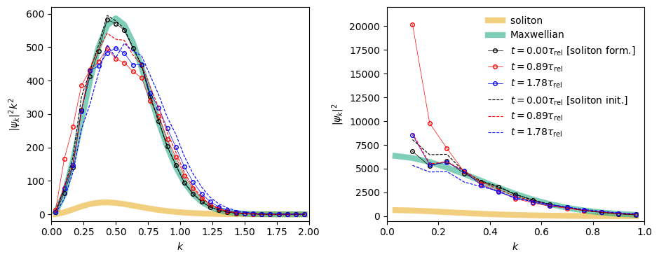
Figure 16: Left panel: Evolution of momentum distribution of axions in the simulation box. The mode amplitudes are spherically averaged over shells with fixed $k=|\mathbf{k}|$. Right panel: Zoom-in on the low-$k$ part of the spectrum, where we divide the distribution by $k^{2}$ to make the difference between curves more pronounced. The distribution in a simulation with spontaneous formation of the soliton from the gas (${\cal N}=128,\,k_{g}=0.5,\,f_{g}=0.06$) is shown by solid lines with circles. It is sampled at three moments of time: at the beginning of the simulation (black), at the time before soliton formation formation (red) and after the soliton has formed (blue). Just before the soliton forms the distribution features a pronounced bump at low momenta which disappears afterwards. For comparison, we show with dashed lines the distribution in a simulation with soliton inserted in the initial conditions ($k_{g}r_{s}^{\rm init}=1.51$) sampled at the same time intervals. Maxwell distribution corresponding to the input gas parameters is shown with thick green line. The momentum wavefunction of the soliton with the mass achieved at latest sampling point is plotted by thick yellow line.

This suggests that the gas distribution restores its Maxwellian form after the soliton formation. We check this conjecture by measuring the amplitudes of axion modes $|\psi_{\mathbf{k}}|^{2}$ in the simulation from fig. 15 at several moments of time: at the beginning of the simulation ($t=0$), before the soliton formation ($t=0.89\,\tau_{\rm rel}$), and after the soliton has formed ($t=1.78\,\tau_{\rm rel}$). The amplitudes are averaged over spherical shells with fixed values of $k=|\mathbf{k}|$. The results are shown in fig. 16 (solid lines with circles). We see that right before the soliton formation, the distribution develops a pronounced bump in the low-$k$ part of the spectrum, consistently with the results of [39]. This bump, however, disappears after the soliton is formed and at late times the distribution qualitatively resembles Maxwellian (shown by the thick green line). We also superimpose in the same figure the distribution for the run with soliton initially present in the gas sampled at the same intervals from the start of the simulation (dashed lines). The parameters of this run are $({\cal N}=128,\,k_{g}=0.5,\,f_{g}=0.06,\,k_{g}r_{s}^{\rm init}=1.51)$ and correspond to the blue curve in fig. 15. In this case we see that the distribution preserves the Maxwellian shape at all times, without any excess at low-$k$ modes. We conclude that the presence of the soliton affects the axion gas in a curious way: it stabilizes the Maxwell distribution of axion momenta.

It is worth stressing that we are talking about the distribution in the gas and not in the soliton itself. Though our numerical procedure does not allow us to separate the two, we can compare the total distribution to the wavefunction of the soliton in momentum space. This is shown by thick yellow line in fig. 16. We take the soliton mass to be $M_{s}=20$ corresponding to the latest sampling time. We see that the contamination of the distribution from the soliton is negligible.

We do not attempt to explore this “Maxwellization” phenomenon further in this work. The axion momentum distribution is subject to significant temporal fluctuations which form an obstruction for moving beyond qualitative statements. For a quantitative study, one needs to devise less noisy probes. We leave this task for future.

Appendix C Details of the numerical simulations

C.1 Convergence tests

In this work, we adopt second order drift-kick-drift operator (4.2) to evolve wave function for each time step ${\rm d}t$. The gravitational potential $\Phi$ and kinetic energy operators $\Delta$ are calculated with CUDA Fast Fourier Transform (cuFFT). We notice that the single precision of cuFFT causes $\approx 10\%$ mass loss in $10^{6}$ time steps. We therefore conduct the simulations in this work using the double precision. This makes the mass loss negligible (less than $10^{-6}$).

The requirement that the gas and the soliton must be resolved by the spatial lattice puts and upper bound on the gas momentum $k_{g}$ and a lower bound on the initial soliton size $r_{s}^{\rm init}$ accessible in the simulations. To determine the domain of validity of our code, we perform several convergence tests. First, we evolve the gas without the soliton using three different time steps: ${\rm d}t=2/\pi\simeq 0.64$ (our fiducial value), ${\rm d}t=1/\pi\simeq 0.32$ and ${\rm d}t=1/(2\pi)\simeq 0.16$. The gas parameters in all three runs are $({\cal N}=128,\,k_{g}=0.5,\,f_{g}=0.04)$. The maximal density within the box and the total energy measured in these runs are shown in the left panel of fig. 17. We observe that the density curves essentially coincide, while the energy error is proportional to $({\rm d}t)^{2}$, as it should. For our fiducial value of ${\rm d}t=2/\pi$, the error stays well below $10^{-7}$. We conclude that the gas with $k_{g}=0.5$ is comfortably resolved in our simulations.

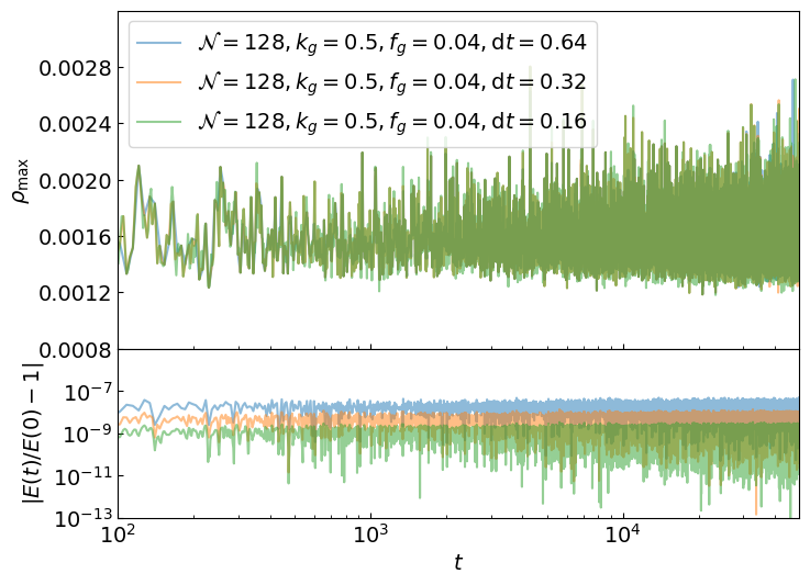
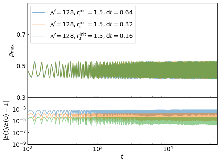
Figure 17: Convergence tests in the simulations with pure gas (left) and an isolated soliton (right). In each case we perform three runs: one with the fiducial time step ${\rm d}t=0.64$, and two with time steps reduced by a factor of 2 and 4. The gas momentum is $k_{g}=0.5$, whereas the soliton radius is $r_{s}^{\rm init}=1.5$. The lattice size if ${\cal N}=128$ in both cases.

Next, we repeat the same convergence test with an isolated soliton of radius $r_{s}^{\rm init}=1.5$. The results are shown in the right panel of fig. 17. Since the analytical template (2.9) used in the simulations to set the initial conditions slightly deviates from the exact soliton profile, the soliton is initiated in an excited state which leads to the oscillations of the peak density. The oscillations obtained with three different time steps match almost identically. The energy error also exhibits the proper scaling, $|E(t)/E(0)-1|\propto({\rm d}t)^{2}$. However, now it is significantly larger, reaching up to $10^{-3}$ for the fiducial ${\rm d}t$. This is likely due to high frequency of the soliton phase rotation $|\mathcal{E}_{s}|\simeq 0.52$ which is less resolved with the large time step. Therefore, to correctly capture the evolution of the soliton wavefunction, we restrict our simulations to $r_{s}^{\rm init}\geq 1.5$.

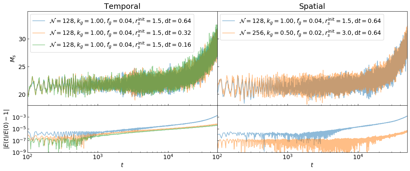
Figure 18: Temporal (left) and spatial (right) convergence tests for the extreme values of the gas momentum and soliton radius $k_{g}=1$, $r_{s}^{\rm init}=1.5$. Temporal test contains three simulations by decreasing the time step size ${\rm d}t$ by 2 or 4 relative to the fiducial value, whereas the spatial test consists of two simulations with the box size ${\cal N}$ differing by a factor of 2. The simulations for spatial test follow the scaling relation (2.2).

For a third test, we superimpose the soliton and the gas and again run three simulations with decreasing time step. We take the soliton with $r_{s}^{\rm init}=1.5$ and push the gas momentum up to $k_{g}=1$. The evolution of the soliton mass and the total energy in these runs is shown in the left panel of fig. 18. The soliton mass growth in the three cases is broadly the same, though detailed features are slightly different. The energy error is low in the initial time range $t\lesssim 10^{3}$ where it also obeys the $({\rm d}t)^{2}$ scaling. However, from $t\sim 10^{3}$ it starts to steadily grow and its scaling with $({\rm d}t)^{2}$ gets violated. Still, the error remains small until very late times. For the fiducial time step it reaches $10^{-3}$ when the soliton mass exceeds $M_{s}\simeq 27$ and hence its radius drops below $r_{s}\simeq 1.2$. This suggests that the soliton-gas system with $r_{s}\sim 1.2$ and $k_{g}\sim 1$ is at the extreme of our numerical resolution. Since we are interested in the averaged properties of the soliton evolution, rather than fine details, we accept $k_{g}=1$ as the upper boundary for admissible gas momenta. To ensure the absence of any excessive loss of precision, we monitor the energy conservation throughout our simulations and only use data where the energy is conserved with accuracy better than $10^{-3}$.

Finally, we perform a spatial convergence test. Instead of varying ${\rm d}x$, which is fixed to $1$ in our code, we make use of the scaling symmetry (2.2). It implies that decreasing ${\rm d}x$ is equivalent to an increase of ${\cal N}$ accompanied by an appropriate rescaling of other parameters. Thus we consider two simulation runs with $({\cal N}=128,\,k_{g}=1,\,f_{g}=0.04,\,r_{s}^{\rm init}=1.5)$ and $({\cal N}=256,\,k_{g}=0.5,\,f_{g}=0.02,\,r_{s}^{\rm init}=3.0)$. Note that we do not rescale the time step ${\rm d}t=2/\pi$ which is tied to the lattice spacing in order to avoid aliasing [35]. The results of these two runs are compared in the right panel of fig. 18. While energy conservation is much better satisfied on the bigger lattice, the broad features of the mass evolution in these two runs agree. This further support the validity of our numerical results up to the extreme values $k_{g}=1$, $r_{s}^{\rm init}=1.5$.

C.2 Conversion of peak density into soliton mass

As discussed in section 4.1, we estimate the mass of the soliton and its radius from the maximal density in the box $\rho_{\rm max}$, assuming that it corresponds to the soliton peak density $\rho_{s,\,{\rm peak}}$. However, the interference of the soliton wavefunction with the gas waves can increase the maximal density above that of the soliton. The increase is proportional to the product of the soliton and gas wavefunctions, hence to the geometric mean of their densities. In more detail, we can estimate the bias as

$$\frac{\rho_{\rm max}}{\rho_{s,\,{\rm peak}}}-1\sim 2\sqrt{\frac{\rho_{g}}{\rho_{s,\,{\rm peak}}}}\;,$$ (C.1)

which can be significant even for large density contrasts. For example, the density bias is about $40\%$ for $\rho_{s,\,{\rm peak}}/\rho_{g}=30$. The situation is further complicated by large fluctuations in the local gas density that can further increase the bias. In particular, when the soliton is too light, its peak becomes completely obscured by the gas.

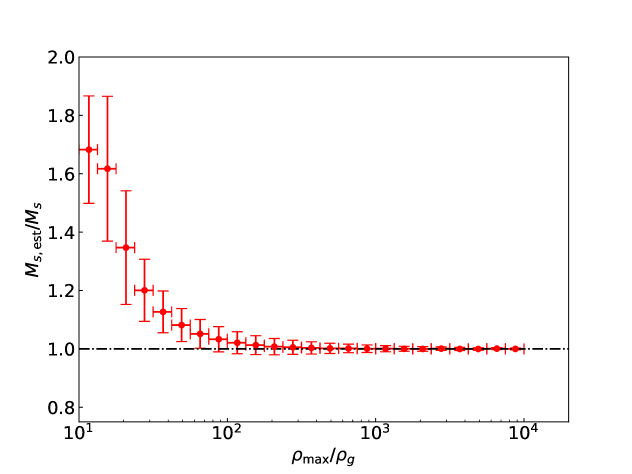
Figure 19: Ratio of the soliton mass estimator to the true soliton mass as functon of the density contrast in the axion field generated by superposition of the soliton and gas wavefunctions. We adopt the threshold $\rho_{\rm max}>30\,\rho_{g}$ when measuring the soliton mass from the simulations.

To pin down the lowest density contrast between the soliton and the gas for which the bias is unimportant, we conduct a series of the following auxiliary numerical experiments. We generate a gas field with given mean density $\rho_{g}$ and superimpose on it a soliton of mass $M_{s}$ without any evolution. Then we evaluate the estimator of the soliton mass using our formula

$$M_{s,{\rm est}}=25.04\,\rho_{\rm max}^{1/4}\;,$$ (C.2)

where $\rho_{\rm max}$ is the maximal density of the axion field in the box. The estimator is compared to the true soliton mass in fig. 19. We observe that when the soliton is prominent enough, say $\rho_{s,\,{\rm peak}}\simeq\rho_{\rm max}>100\,\rho_{g}$, the estimator is unbiased. On the other hand, for $\rho_{\rm max}\lesssim 20\,\rho_{g}$, we are essentially unable to distinguish the soliton peak against the gas density fluctuations. We adopt the threshold $\rho_{\rm max}>30\,\rho_{g}$ when measuring the soliton mass in our simulations, which introduces an error of at most 20% in the mass estimate.

References

- [1] S. Weinberg, A New Light Boson?, Phys. Rev. Lett. 40 (1978) 223.
- [2] F. Wilczek, Problem of Strong and Invariance in the Presence of Instantons, Phys. Rev. Lett. 40 (1978) 279.
- [3] M. A. Shifman, A. I. Vainshtein and V. I. Zakharov, Can Confinement Ensure Natural CP Invariance of Strong Interactions?, Nucl. Phys. B166 (1980) 493.
- [4] J. E. Kim, Weak Interaction Singlet and Strong CP Invariance, Phys. Rev. Lett. 43 (1979) 103.
- [5] A. R. Zhitnitsky, On Possible Suppression of the Axion Hadron Interactions. (In Russian), Sov. J. Nucl. Phys. 31 (1980) 260 [Yad. Fiz.31,497(1980)].
- [6] M. Dine, W. Fischler and M. Srednicki, A Simple Solution to the Strong CP Problem with a Harmless Axion, Phys. Lett. 104B (1981) 199.
- [7] J. Preskill, M. B. Wise and F. Wilczek, Cosmology of the Invisible Axion, Phys. Lett. 120B (1983) 127.
- [8] L. F. Abbott and P. Sikivie, A Cosmological Bound on the Invisible Axion, Phys. Lett. 120B (1983) 133.
- [9] M. Dine and W. Fischler, The Not So Harmless Axion, Phys. Lett. 120B (1983) 137.
- [10] A. Arvanitaki, S. Dimopoulos, S. Dubovsky, N. Kaloper and J. March-Russell, String Axiverse, Phys. Rev. D81 (2010) 123530 [0905.4720].
- [11] D. J. E. Marsh, Axion Cosmology, Phys. Rept. 643 (2016) 1 [1510.07633].
- [12] L. Hui, J. P. Ostriker, S. Tremaine and E. Witten, Ultralight scalars as cosmological dark matter, Phys. Rev. D95 (2017) 043541 [1610.08297].
- [13] L. Hui, Wave Dark Matter, Ann. Rev. Astron. Astrophys. 59 (2021) 247 [2101.11735].
- [14] R. D. Peccei and H. R. Quinn, CP Conservation in the Presence of Instantons, Phys. Rev. Lett. 38 (1977) 1440.
- [15] R. D. Peccei and H. R. Quinn, Constraints Imposed by CP Conservation in the Presence of Instantons, Phys. Rev. D16 (1977) 1791.
- [16] P. Svrcek and E. Witten, Axions In String Theory, JHEP 06 (2006) 051 [hep-th/0605206].
- [17] W. Hu, R. Barkana and A. Gruzinov, Cold and fuzzy dark matter, Phys. Rev. Lett. 85 (2000) 1158 [astro-ph/0003365].
- [18] E. Armengaud, N. Palanque-Delabrouille, C. Yèche, D. J. E. Marsh and J. Baur, Constraining the mass of light bosonic dark matter using SDSS Lyman- forest, Mon. Not. Roy. Astron. Soc. 471 (2017) 4606 [1703.09126].
- [19] T. Kobayashi, R. Murgia, A. De Simone, V. Iršič and M. Viel, Lyman- constraints on ultralight scalar dark matter: Implications for the early and late universe, Phys. Rev. D 96 (2017) 123514 [1708.00015].
- [20] K. K. Rogers and H. V. Peiris, Strong Bound on Canonical Ultralight Axion Dark Matter from the Lyman-Alpha Forest, Phys. Rev. Lett. 126 (2021) 071302 [2007.12705].
- [21] N. Bar, D. Blas, K. Blum and S. Sibiryakov, Galactic rotation curves versus ultralight dark matter: Implications of the soliton-host halo relation, Phys. Rev. D 98 (2018) 083027 [1805.00122].
- [22] N. Bar, K. Blum and C. Sun, Galactic rotation curves versus ultralight dark matter: A systematic comparison with SPARC data, Phys. Rev. D 105 (2022) 083015 [2111.03070].
- [23] M. Safarzadeh and D. N. Spergel, Ultra-light Dark Matter is Incompatible with the Milky Way’s Dwarf Satellites, 1906.11848.
- [24] S. L. Zoutendijk, J. Brinchmann, N. F. Bouché, M. d. Brok, D. Krajnović, K. Kuijken et al., The MUSE-Faint survey - II. The dark-matter density profile of the ultra-faint dwarf galaxy Eridanus 2, Astron. Astrophys. 651 (2021) A80 [2101.00253].
- [25] DES collaboration, E. O. Nadler et al., Milky Way Satellite Census. III. Constraints on Dark Matter Properties from Observations of Milky Way Satellite Galaxies, Phys. Rev. Lett. 126 (2021) 091101 [2008.00022].
- [26] D. J. E. Marsh and J. C. Niemeyer, Strong Constraints on Fuzzy Dark Matter from Ultrafaint Dwarf Galaxy Eridanus II, Phys. Rev. Lett. 123 (2019) 051103 [1810.08543].
- [27] N. Dalal and A. Kravtsov, Not so fuzzy: excluding FDM with sizes and stellar kinematics of ultra-faint dwarf galaxies, 2203.05750.
- [28] R. Ruffini and S. Bonazzola, Systems of selfgravitating particles in general relativity and the concept of an equation of state, Phys. Rev. 187 (1969) 1767.
- [29] F. S. Guzman and L. A. Urena-Lopez, Gravitational cooling of self-gravitating Bose-Condensates, Astrophys. J. 645 (2006) 814 [astro-ph/0603613].
- [30] C. J. Hogan and M. J. Rees, Axion miniclusters, Phys. Lett. B205 (1988) 228.
- [31] E. W. Kolb and I. I. Tkachev, Axion miniclusters and Bose stars, Phys. Rev. Lett. 71 (1993) 3051 [hep-ph/9303313].
- [32] H.-Y. Schive, T. Chiueh and T. Broadhurst, Cosmic Structure as the Quantum Interference of a Coherent Dark Wave, Nature Phys. 10 (2014) 496 [1406.6586].
- [33] J. Veltmaat, J. C. Niemeyer and B. Schwabe, Formation and structure of ultralight bosonic dark matter halos, Phys. Rev. D 98 (2018) 043509 [1804.09647].
- [34] M. Mina, D. F. Mota and H. A. Winther, Solitons in the dark: non-linear structure formation with fuzzy dark matter, 2007.04119.
- [35] S. May and V. Springel, Structure formation in large-volume cosmological simulations of fuzzy dark matter: impact of the non-linear dynamics, Mon. Not. Roy. Astron. Soc. 506 (2021) 2603 [2101.01828].
- [36] H.-Y. Schive, M.-H. Liao, T.-P. Woo, S.-K. Wong, T. Chiueh, T. Broadhurst et al., Understanding the Core-Halo Relation of Quantum Wave Dark Matter from 3D Simulations, Phys. Rev. Lett. 113 (2014) 261302 [1407.7762].
- [37] B. Schwabe, J. C. Niemeyer and J. F. Engels, Simulations of solitonic core mergers in ultralight axion dark matter cosmologies, Phys. Rev. D 94 (2016) 043513 [1606.05151].
- [38] P. Mocz, M. Vogelsberger, V. H. Robles, J. Zavala, M. Boylan-Kolchin, A. Fialkov et al., Galaxy formation with BECDM – I. Turbulence and relaxation of idealized haloes, Mon. Not. Roy. Astron. Soc. 471 (2017) 4559 [1705.05845].
- [39] D. G. Levkov, A. G. Panin and I. I. Tkachev, Gravitational Bose-Einstein condensation in the kinetic regime, Phys. Rev. Lett. 121 (2018) 151301 [1804.05857].
- [40] T. D. Yavetz, X. Li and L. Hui, Construction of wave dark matter halos: Numerical algorithm and analytical constraints, Phys. Rev. D 105 (2022) 023512 [2109.06125].
- [41] J. F. Navarro, C. S. Frenk and S. D. M. White, A Universal density profile from hierarchical clustering, Astrophys. J. 490 (1997) 493 [astro-ph/9611107].
- [42] B. Eggemeier and J. C. Niemeyer, Formation and mass growth of axion stars in axion miniclusters, Phys. Rev. D 100 (2019) 063528 [1906.01348].
- [43] H.-Y. Schive, T. Chiueh and T. Broadhurst, Soliton Random Walk and the Cluster-Stripping Problem in Ultralight Dark Matter, Phys. Rev. Lett. 124 (2020) 201301 [1912.09483].
- [44] X. Li, L. Hui and T. D. Yavetz, Oscillations and Random Walk of the Soliton Core in a Fuzzy Dark Matter Halo, Phys. Rev. D 103 (2021) 023508 [2011.11416].
- [45] J. Luna Zagorac, I. Sands, N. Padmanabhan and R. Easther, Schrödinger-Poisson Solitons: Perturbation Theory, arXiv e-prints (2021) arXiv:2109.01920 [2109.01920].
- [46] H. Y. J. Chan, E. G. M. Ferreira, S. May, K. Hayashi and M. Chiba, The diversity of core–halo structure in the fuzzy dark matter model, Mon. Not. Roy. Astron. Soc. 511 (2022) 943 [2110.11882].
- [47] M. Nori and M. Baldi, Scaling relations of fuzzy dark matter haloes – I. Individual systems in their cosmological environment, Mon. Not. Roy. Astron. Soc. 501 (2021) 1539 [2007.01316].
- [48] J. Chen, X. Du, E. W. Lentz, D. J. E. Marsh and J. C. Niemeyer, New insights into the formation and growth of boson stars in dark matter halos, Phys. Rev. D 104 (2021) 083022 [2011.01333].
- [49] J. H. H. Chan, H.-Y. Schive, T.-P. Woo and T. Chiueh, How do stars affect DM haloes?, MNRAS 478 (2018) 2686 [1712.01947].
- [50] J. Veltmaat, B. Schwabe and J. C. Niemeyer, Baryon-driven growth of solitonic cores in fuzzy dark matter halos, Phys. Rev. D 101 (2020) 083518 [1911.09614].
- [51] B. T. Chiang, H.-Y. Schive and T. Chiueh, Soliton Oscillations and Revised Constraints from Eridanus II of Fuzzy Dark Matter, Phys. Rev. D 103 (2021) 103019 [2104.13359].
- [52] D. D. Chowdhury, F. C. van den Bosch, V. H. Robles, P. van Dokkum, H.-Y. Schive, T. Chiueh et al., On the Random Motion of Nuclear Objects in a Fuzzy Dark Matter Halo, Astrophys. J. 916 (2021) 27 [2105.05268].
- [53] D. G. Levkov, A. G. Panin and I. I. Tkachev, Relativistic axions from collapsing Bose stars, Phys. Rev. Lett. 118 (2017) 011301 [1609.03611].
- [54] I. I. Tkachev, Fast Radio Bursts and Axion Miniclusters, JETP Lett. 101 (2015) 1 [1411.3900].
- [55] M. P. Hertzberg and E. D. Schiappacasse, Dark Matter Axion Clump Resonance of Photons, JCAP 11 (2018) 004 [1805.00430].
- [56] D. G. Levkov, A. G. Panin and I. I. Tkachev, Radio-emission of axion stars, Phys. Rev. D 102 (2020) 023501 [2004.05179].
- [57] B. J. Kavanagh, T. D. P. Edwards, L. Visinelli and C. Weniger, Stellar disruption of axion miniclusters in the Milky Way, Phys. Rev. D 104 (2021) 063038 [2011.05377].
- [58] D. Ellis, D. J. E. Marsh, B. Eggemeier, J. Niemeyer, J. Redondo and K. Dolag, Structure of axion miniclusters, Phys. Rev. D 106 (2022) 103514 [2204.13187].
- [59] B. Eggemeier, B. Schwabe, J. C. Niemeyer and R. Easther, Gravitational collapse in the postinflationary Universe, Phys. Rev. D 105 (2022) 023516 [2110.15109].
- [60] X. Du, B. Schwabe, J. C. Niemeyer and D. Bürger, Tidal disruption of fuzzy dark matter subhalo cores, Phys. Rev. D 97 (2018) 063507 [1801.04864].
- [61] P.-H. Chavanis, Landau equation for self-gravitating classical and quantum particles: application to dark matter, Eur. Phys. J. Plus 136 (2021) 703 [2012.12858].
- [62] J. Chan, S. Sibiryakov and W. Xue, in preparation.
- [63] F. S. Guzman and L. A. Urena-Lopez, Evolution of the Schrodinger-Newton system for a selfgravitating scalar field, Phys. Rev. D 69 (2004) 124033 [gr-qc/0404014].
- [64] L. Pitaevskii and S. Stringari, Bose-Einstein Condensation and Superfluidity, International Series of Monographs on Physics. OUP Oxford, 2016.
- [65] C. K. Birdsall and A. B. Langdon, Plasma physics via computer simulation. CRC press, 2018.
- [66] F. S. Guzmán, Oscillation modes of ultralight BEC dark matter cores, Phys. Rev. D 99 (2019) 083513 [1812.11612].
- [67] E. W. Kolb and I. I. Tkachev, Large amplitude isothermal fluctuations and high density dark matter clumps, Phys. Rev. D 50 (1994) 769 [astro-ph/9403011].