Few-Example Clustering via Contrastive Learning

Abstract

We propose Few-Example Clustering (FEC), a novel algorithm that performs contrastive learning to cluster few examples. Our method is composed of the following three steps: (1) generation of candidate cluster assignments, (2) contrastive learning for each cluster assignment, and (3) selection of the best candidate. Based on the hypothesis that the contrastive learner with the ground-truth cluster assignment is trained faster than the others, we choose the candidate with the smallest training loss in the early stage of learning in step (3). Extensive experiments on the mini-ImageNet and CUB-200-2011 datasets show that FEC outperforms other baselines by about 3.2% on average under various scenarios. FEC also exhibits an interesting learning curve where clustering performance gradually increases and then sharply drops.

1 Introduction

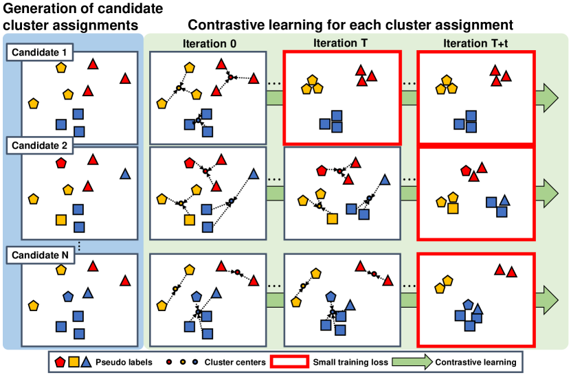
Figure 1: A conceptual illustration of our proposed algorithm FEC in the feature space. The same shape indicates the same ground-truth cluster. For each cluster assignment, we fine-tune the feature network using contrastive learning that minimizes the distance between the examples within the same cluster and maximizes the distance between the examples from different clusters in the feature space. We regard the candidate with the smallest training loss in the early stage of learning as the best candidate. In this figure, since the candidate 1 converges faster than the other candidates, we choose the candidate 1 as the best one.

Clustering, which is one of the most popular unsupervised techniques, aims to group similar examples into the same cluster by a similarity measure. Although conventional clustering methods such as K-means clustering (MacQueen, 1967) are powerful on a large-scale dataset, they are ineffective for High Dimension, Low Sample Size (HDLSS) examples. (Ahn et al., 2012; Terada, 2013; Sarkar & Ghosh, 2020; Shen et al., 2021). Studies on clustering HDLSS data can be helpful for many applications, including neurological diseases analysis (Datta & Datta, 2003; Liu et al., 2008; Alashwal et al., 2019).

Recently, deep learning techniques have achieved great progress in a variety of areas including visual recognition and language translation (Krizhevsky et al., 2012; Simonyan & Zisserman, 2015; Devlin et al., 2019). However, to the best of our knowledge, not much progress has been made in utilizing deep neural networks on clustering HDLSS data.

In this paper, we propose Few-Example Clustering (FEC), a novel clustering algorithm based on the hypothesis that the contrastive learner with the ground-truth cluster assignment is trained faster than the others. This hypothesis is built on the phenomenon that deep neural networks initially learn patterns from the training examples. FEC is composed of the following three steps (see Figure 1): (1) generation of candidate cluster assignments, (2) contrastive learning for each cluster assignment, and (3) selection of the best candidate. In step (1), we generate candidate cluster assignments using a pre-trained feature network. In step (2), for each candidate, we fine-tune the feature network using contrastive learning that minimizes the distance between examples in the same cluster and maximizes the distance between examples from different clusters in the feature space. Based on the hypothesis mentioned earlier, we choose the candidate with the smallest training loss in the early stage of learning in step (3).

We investigate the effectiveness of FEC under various scenarios on the mini-ImageNet and CUB-200-2011 datasets. We evaluate on the task to group five examples into two clusters of sizes one and four. FEC outperforms other baselines by about 3.2% on average in accuracy. We further evaluate on the task to group 80 examples into 5 clusters. FEC outperforms other baselines by about 0.013 and 0.018 on average in Adjusted Rand Index (ARI) and Normalized Mutual Information (NMI), respectively.

2 Related works

Training dynamics of DNNs: Arpit et al. (2017) showed that deep neural networks (DNNs) initially learn patterns from the training examples during training. In the presence of label noise, the examples with noisy labels do not share the patterns of the examples with clean labels. Based on the phenomenon, some studies regard the examples that have small losses in the initial phase of learning as examples with clean labels (Jiang et al., 2017; Han et al., 2018; Lee & Chung, 2019).

Inspired by the small-loss criterion to find clean examples, we regard the candidate with the smallest training loss in the early stage of learning as the best candidate in step (3) of our algorithm.

Self-supervised learning: Our method is related to two self-supervised approaches: deep clustering and contrastive learning.

Deep clustering that combines clustering and representation learning is one of the most promising approaches for self-supervised learning (Xie et al., 2016; Caron et al., 2018; Asano et al., 2019; Ji et al., 2019; Sharma et al., 2020). Most studies in this approach iteratively (1) perform clustering methods such as K-means for pseudo-labeling on unlabeled examples and (2) learn representation using supervised learning with the pseudo labels. Deep clustering has shown comparative representation learning performance to supervised learning.

Contrastive learning aims to learn representations by minimizing the distances between positive (i.e., similar) pairs and maximizing the distance between negative (i.e., dissimilar) pairs. The positive and negative pairs can be generated by data augmentation (Chen et al., 2020; Grill et al., 2020; Khosla et al., 2020) or they can be identified by clustering methods such as K-means in guided SimCLR (Chakraborty et al., 2020; Li et al., 2020; Sharma et al., 2020). Recently, contrastive learning methods have shown state-of-the-art performance in self-supervised learning.

Few-shot learning: Learning in a few-data regime has been largely discussed in the context of classification (Ravi & Larochelle, 2017; Chen et al., 2019). One direction of few-shot learning research is inductive few-shot learning, which uses labeled examples to adapt a classifier to the novel task. Some studies in this direction are based on metric learning. The approaches, which seek to learn embeddings with good generalization ability (Vinyals et al., 2016; Snell et al., 2017), task-adaptive metric (Oreshkin et al., 2018; Sung et al., 2018), and task-adaptive embeddings (Yoon et al., 2019; Lichtenstein et al., 2020). Other studies in this direction are gradient-based approaches, which seek to find an initialization that facilitates few-shot adaptation (Finn et al., 2017; Nichol et al., 2018; Rusu et al., 2019). Another direction of few-shot learning research is transductive few-shot learning, which uses not only labeled examples but also unlabeled examples to adapt a classifier to the novel task. Most studies in this direction are based on label propagation (Liu et al., 2018; Qiao et al., 2019).

Sinkhorn K-means clustering: Sinkhorn K-means clustering (Asano et al., 2019; Genevay et al., 2019; Huang et al., 2019) is a variant of K-means that regards K-means clustering as an optimal transportation problem and finds cluster assignment by using the Sinkhorn-Knopp algorithm under the constraint that cluster sizes are equal. i.e., Sinkhorn K-means clustering aims to cluster $N$ examples $\{x_{1},x_{2},\cdots,x_{N}\}$ into $K$ clusters. Sinkhorn K-means to get the assignment $p$ is formulated as follows:

$$\min_{p,\mu} \sum_{j=1}^{K}\sum_{i=1}^{N}p_{i,j}d(x_{i},\mu_{j})-\gamma H(p)$$ (1)

s.t. $$\sum_{j=1}^{K}p_{i,j}=\frac{1}{N},\forall i\in\{1,\ldots,N\}$$ (2)

$$\sum_{i=1}^{N}p_{i,j}=\frac{1}{K},\forall j\in\{1,\ldots,K\}$$ (3)

$$0\leq p_{i,j}\leq 1,$$ (4)

where $H(p)$ denotes the entropy of the assignment $p$, $\mu_{k}$ denotes the center of the $k$-th cluster determined by the assignment $p$, and $\gamma$ denotes a hyperparameter for the entropy term. More details on Sinkhorn K-means clustering will be described in Appendix A.

3 Methodology

Algorithm 1 FEC with exhaustive search

  Input: pre-trained feature model $f_{\theta}$, unlabeled dataset $\mathcal{D}$, number of clusters $N$, size of each cluster $K$, number of candidates $N_{c}$, softmax temperature $\alpha$

  Consider all possible cluster assignments as candidates

  Generate randomly initialized additional layers $g_{\phi}^{c}$ for each candidate $c$

  repeat

     for $p=1$ to $N_{c}$ do

        Train $g_{\phi}^{c}$ to minimize the loss $\mathcal{L}(\mathcal{D}^{c};\phi,\alpha)$ in (5)

     end for

  until training loss of the best candidate is converged

  Choose the candidate $c^{*}$ that has the smallest training loss.

Algorithm 2 FEC with iterative partial search

  Input: pre-trained feature model $f_{\theta}$, unlabeled dataset $\mathcal{D}$, number of clusters $N$, number of candidates $N_{c}$, duration of fine-tuning $T_{f}$, assignment refinement period $T_{r}$, softmax temperature $\alpha$, clustering method $\mathcal{E}$

  Generate $N_{c}$ candidate cluster assignments by running the clustering algorithm $\mathcal{E}$ multiple times in the feature space $f_{\theta}$

  Generate randomly initialized additional layers $g_{\phi}^{c}$ for each candidate $c$

  for $t=1$ to $T_{f}$ do

     for $c=1$ to $N_{c}$ do

        Train $g_{\phi}^{c}$ to minimize the loss $\mathcal{L}(\mathcal{D}^{c};\phi,\alpha)$ in (5)

        if $t\equiv-1\pmod{T_{r}}$ then

           Refine the candidate cluster assignment $c$ by running the clustering algorithm $\mathcal{E}$ in the feature space $g_{\phi}^{c}\circ f_{\theta}$

           Re-initialize the additional layers $g_{\phi}^{c}$

        end if

     end for

  end for

  Choose the candidate $c^{*}$ that has the smallest training loss.

3.1 Problem statement

Suppose that a pre-trained feature model $f_{\theta}$ is given. Let $\mathcal{D}=\{x_{1},x_{2},\cdots,x_{N}\}$ denote a dataset consisting of $N$ unlabeled examples. Our goal is to cluster $N$ examples in the dataset $\mathcal{D}$ into $K$ clusters.

3.2 FEC with exhaustive search

FEC with exhaustive search is composed of three steps as detailed in Algorithm 1: (1) generation of candidate cluster assignments, (2) contrastive learning for each cluster assignment, and (3) selection of the best candidate.

Generation of candidate cluster assignments: We consider all possible cluster assignments as candidate cluster assignments.

Contrastive learning for each cluster assignment: For each candidate, we fine-tune the feature network using contrastive learning that minimizes the distance between examples in the same cluster and maximizes the distance between examples from different clusters in the feature space.

For each candidate cluster assignment $c$, we assign pseudo labels to the unlabeled examples as $\mathcal{D}^{c}:=\{(x_{i},l^{c}_{i})|1\leq i\leq N\}$, where $l_{i}^{c}$ is the pseudo label of $x_{i}$ determined by the candidate $c$. To fine-tune feature models using contrastive learning, we freeze the pre-trained network $f_{\theta}$ and add new trainable layers $g_{\phi}^{c}$ on top of $f_{\theta}$. With a metric $d$, we minimize the distance between an example $x$ and the center of the cluster $x$ belongs to and maximize the distance between the example and the other cluster centers in the feature space of $g_{\phi}^{c}\circ f_{\theta}$. i.e., we minimize the following loss

$$\begin{split}\min_{\phi}\;&\mathcal{L}(\mathcal{D}^{c};\phi,\alpha)\\ &=\sum_{k=1}^{K}\sum_{(x_{i},l_{i}^{c}=k)\in\mathcal{D}^{c}}\frac{\exp(-\alpha d(g_{\phi}^{c}\circ f_{\theta}(x_{i}),\mu_{k}^{c}))}{\sum_{j}\exp(-\alpha d(g_{\phi}^{c}\circ f_{\theta}(x_{i}),\mu_{j}^{c}))},\end{split}$$ (5)

where $\alpha$ denotes the softmax temperature and $\mu_{k}^{c}$ denotes the center of the $k$-th cluster determined by the candidate $c$. In addition, we use an ensemble method to reduce the influences caused by random initializations of additional layers.

Selection of the best candidate: To select the best candidate, we hypothesize that the contrastive learner with the ground-truth cluster assignment is trained faster than the others. This hypothesis is built on the phenomenon that deep neural networks learn patterns from the training examples in the early stage of training. Based on the hypothesis, we choose the candidate with the smallest training loss in the early stage of learning. Therefore, we need an early stopping criterion. We terminate learning when the training loss of the best candidate converges (i.e. when the decrease in training loss is less than a threshold $\delta$).

3.3 FEC with iterative partial search

FEC with iterative partial search differs from FEC with exhaustive search in two aspects: (1) FEC with iterative partial search deals with a small subset of all possible cluster assignments and (2) iteratively performs contrastive learning and cluster assignment refinement (see Algorithm 2).

Since the number of all possible cluster assignments exponentially increases as the number of examples increases, FEC with exhaustive search is impossible when the number of examples is large. Therefore, we only deal with $N_{c}$ candidate cluster assignments in FEC with iterative partial search.

Deep clustering methods (Caron et al., 2018; Asano et al., 2019; Ji et al., 2019) improve cluster assignment by iteratively performing clustering methods on the learned feature space to generate pseudo labels and adapting representations using supervised learning with the pseudo labels. Inspired by the iterative updates in deep clustering methods, we refine the candidate cluster assignments on the feature space periodically in FEC with iterative partial search.

Both FEC with iterative partial search and FEC with exhaustive search select the best candidate based on the same hypothesis mentioned earlier. Thus, FEC with iterative partial search also needs an early stopping criterion. We tried several early stopping criteria for FEC with iterative partial search, but it was the most effective to terminate after a fixed number of iterations for all tasks.

In addition, we use an ensemble method to reduce the influence caused by random initializations of additional layers. For each cluster assignment, ensemble members are trained in parallel. Even with the same training examples, all members show different clustering outcomes due to random initializations. When we refine the cluster assignment, we choose the ensemble member with the smallest training loss and refine the assignment in the learned feature space of the chosen member. Then, we synchronize all the cluster assignments of members with the refined cluster assignments. The ensemble version of FEC with iterative partial search is described in Appendix D.

4 Experiments

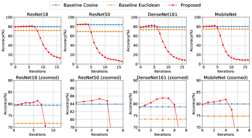
Figure 2: Training curves of FEC on 4:1 clustering task under the scenario mini-ImageNet$\rightarrow$CUB. The clustering accuracy reaches peaks at the early stage of learning. However, as the learning continues, the accuracy sharply drops.

Table 1: Average accuracy(%) on the 4:1 clustering task under different three scenarios: mini-ImageNet$\rightarrow$mini-ImageNet, mini-ImageNet$\rightarrow$CUB, and ImageNet$\rightarrow$CUB. Our proposed FEC outperforms all baselines under vairous scenarios.

Method	Backbone	Accuracy (%)
		mini $\rightarrow$ mini	mini $\rightarrow$ CUB	ImageNet $\rightarrow$ CUB
Euclidean	ResNet18	62.7	47.2	71.4
Cosine	ResNet18	73.5	50.0	79.4
PCA+Euclidean	ResNet18	62.7	47.8	71.7
PCA+Cosine	ResNet18	73.5	51.4	79.4
FEC (Proposed)	ResNet18	76.9	53.1	82.0
Euclidean	ResNet50	52.0	42.4	69.3
Cosine	ResNet50	57.2	45.2	83.9
PCA+Euclidean	ResNet50	52.2	43.9	70.0
PCA+Cosine	ResNet50	58.7	46.2	83.9
FEC (Proposed)	ResNet50	63.0	48.4	88.9
Euclidean	DenseNet	63.9	50.7	73.5
Cosine	DenseNet	74.7	53.5	78.7
PCA+Euclidean	DenseNet	64.8	50.7	73.5
PCA+Cosine	DenseNet	75.0	53.7	78.7
FEC (Proposed)	DenseNet	75.6	55.4	84.4
Euclidean	MobileNet	64.1	51.4	74.7
Cosine	MobileNet	74.1	54.0	79.9
PCA+Euclidean	MobileNet	64.1	52.2	74.8
PCA+Cosine	MobileNet	74.2	54.4	80.5
FEC (Proposed)	MobileNet	77.4	56.6	86.8

In this section, we show the effectiveness of FEC under various scenarios on the mini-ImageNet and CUB-200-2011 datasets. We test on the task to group five examples into two clusters of sizes one and four. We further test on the few-shot learning task when labeled examples are unavailable.

4.1 Experimental setup

Datasets: We consider two widely used datasets in few-shot learning research: the mini-ImageNet (Deng et al., 2009) and CUB-200-2011 (Wah et al., 2011) datasets (hereinafter referred to as CUB). The mini-ImageNet dataset is composed of generic images and used to test generic visual recognition ability. The CUB dataset is composed of bird images and used to test fine-grained image clustering ability. We resize images to $84\times 84$ for mini-ImageNet pre-trained models and to $224\times 224$ for ImageNet pre-trained models. More details on these datasets will be described in Appendix B.

Evaluation scenarios: We test FEC on three different evaluation scenarios motivated from (Chen et al., 2019): generic image clustering scenario (mini-ImageNet $\rightarrow$ mini-ImageNet) and cross-domain clustering scenarios (mini-ImageNet $\rightarrow$ CUB and ImageNet $\rightarrow$ CUB). In the generic image clustering scenario, we cluster generic images from the mini-ImageNet dataset using the mini-ImageNet pre-trained models. In the cross-domain clustering scenarios, we cluster fine-grained images from the CUB dataset using the mini-ImageNet/ImageNet pre-trained models. We remark that the examples in the clustering task are not used for pre-training.

Architectures: We examine FEC with various architectures of the feature models, ResNet18, ResNet50, DenseNet, and MobileNet, which are widely used for ImageNet classification tasks. The additional layers are composed of a single layer and two layers for the experiments in Section 4.2 and Section 4.3, respectively. The output dimension of the additional layers is set to 512. More details on these architectures will be described in Appendix C.

Hyperparameters: FEC with exhaustive search involves three hyperparameters: early stopping threshold $\delta$, softmax temperature $\alpha$, and the number of ensembles $N_{e}$. $\alpha$ is set to 10, $N_{e}$ is set to 32, and $\delta$ is set to $10^{-5}$ for the most experiments and $10^{-3}$ for the experiments using mini-ImageNet pre-trained ResNet50.

FEC with iterative partial search involves four hyperparameters: the period of assignment refinement $T_{r}$ and duration of fine-tuning $T_{s}$, softmax temperature $\alpha$, and the number of ensembles $N_{e}$. $N_{e}$ is set to 5, and $\alpha$ is set to 10. When we use mini-ImageNet pre-trained models, $T_{r}$ and $T_{s}$ are set to 4 and 64, respectively. When we use ImageNet pre-trained models, $T_{r}$ and $T_{s}$ are set to 8 and 16, respectively. More experimental results on other combinations of $T_{s}$ and $T_{r}$ are summarized in Appendix E.

Evaluation metrics for clustering: We use the standard metrics: accuracy, Normalized Mutual Information (NMI), and Adjusted Rand Index (ARI) (Vinh et al., 2010). Accuracy measures how accurately we find the ground-truth cluster assignment when we use FEC with exhaustive search. For FEC with iterative partial search, we use NMI and ARI to measure our clustering quality.

Implementation details: Unless otherwise specified, we use cosine similarity as a similarity measure in our methods. For all experiments, the averaged performances of over 1000 tasks are reported. For pre-trained feature models, we follow the training procedure described in (Wang et al., 2019) and the implementation in PyTorch hub (Paszke et al., 2019) for mini-ImageNet and ImageNet, respectively. To fine-tune the additional layers, we use Adam (Kingma & Ba, 2015) as the optimizer with an initial learning rate of $10^{-3}$.

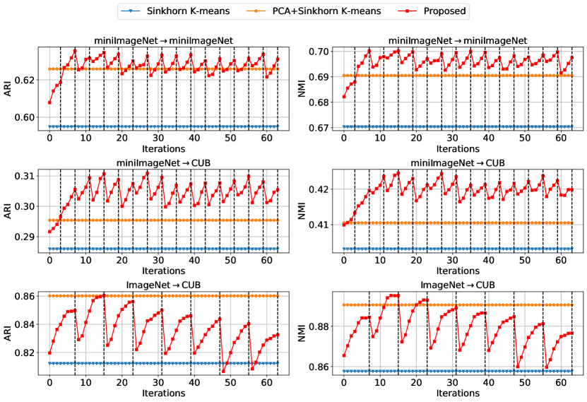
Figure 3: Training curves of FEC+Sinkhorn K-means on the task of clustering 80 examples into 5 clusters with DenseNet. The black dashed lines represent the timings when we refine the pseudo labels.

4.2 4:1 clustering

In this problem, each task consists of only five images $\mathcal{D}=\{x_{1},x_{2},\cdots,x_{5}\}$ with the ground-truth clusters of sizes one and four. 4:1 clustering task is identical to finding the farthest example from the other four examples. i.e., we aim to find $x_{\hat{n}}$ that satisfies

$$\hat{n}=\max_{n\in\{1,2,\ldots,5\}}d\left(h(x_{n}),\frac{1}{4}\sum_{x\in\mathcal{D}_{\mathcal{T}}-x_{n}}h(x)\right),$$ (6)

where $d$ denotes a metric and $h$ denotes a pre-trained feature model. Since there are only five clustering candidates, we use Algorithm 1 for this task. We consider four baselines by combining two metrics, cosine and Euclidean, and two different feature spaces, a fixed feature space and a dimension reduced feature space by Principal Component Analysis (PCA). We call these baselines as cosine, Euclidean, PCA+cosine, and PCA+Euclidean, respectively. For baselines with PCA, we tried principal dimensions from 1 to 4, and the best result among them is reported in Table 1.

The training curves of FEC on the scenario ImageNet $\rightarrow$ CUB can be found in Figure 2. We can observe that the clustering accuracy reaches peaks at the early stage of learning. This observation is consistent with the expectation that the contrastive learner with the ground-truth cluster assignment is learned faster than the others. However, as the learning continues, the accuracy sharply drops, which could be due to over-fitting to non-significant patterns.

The overall experimental results on the 4:1 clustering task are summarized in Table 1. We can observe that the baselines using cosine similarity show better performance than the baselines using Euclidean metric, and PCA does not improve performances of baselines Cosine and Euclidean in this task. Our proposed algorithm FEC substantially outperforms all baselines by about 3% on average in accuracy.

Comparing Figure 2 and Table 1 shows that using different early stopping for each task increased the clustering performance by about 2% rather than stopping after a fixed number of iterations for all tasks.

4.3 Clustering 80 examples into 5 clusters

In this problem, we aim to group 80 examples into 5 clusters of equal sizes. Since the complexity of this problem is high, we use Algorithm 2 instead of Algorithm 1 for this task. We consider three baselines based on K-means clustering: K-means, Sinkhorn K-means, and PCA+Sinkhorn K-means. PCA+Sinkhorn K-means clusters the examples in the task by performing Sinkhorn K-means clustering on the reduced dimension feature space by PCA. For PCA+Sinkhorn K-means, we tried principal dimensions of 2, 4, 8, 16, 32, and 64, and the best result among them is reported in Table 2.

Table 2: Average performance on the task of clustering 80 examples into 5 clusters under three different scenarios: mini-ImageNet$\rightarrow$mini-ImageNet, mini-ImageNet$\rightarrow$CUB, and ImageNet$\rightarrow$CUB. Our proposed FEC+Sinkhorn K-means mostly outperforms all baselines under various scenarios.

Method	Backbone	mini $\rightarrow$ mini		mini $\rightarrow$ CUB		ImageNet $\rightarrow$ CUB
		ARI	NMI	ARI	NMI	ARI	NMI
K-means	ResNet18	0.4654	0.5888	0.2502	0.3810	0.6128	0.7372
Sinkhorn K-means	ResNet18	0.5690	0.6503	0.2779	0.3952	0.7891	0.8358
PCA+Sinkhorn K-means	ResNet18	0.5978	0.6683	0.2840	0.3993	0.8159	0.8538
FEC+Sinkhorn K-means (Proposed)	ResNet18	0.6075	0.6781	0.2963	0.4137	0.8155	0.8607
K-means	ResNet50	0.3322	0.4705	0.2116	0.3354	0.6623	0.7811
Sinkhorn K-means	ResNet50	0.3366	0.4602	0.2231	0.3400	0.8229	0.8655
PCA+Sinkhorn K-means	ResNet50	0.3659	0.4819	0.2275	0.3428	0.8523	0.8845
FEC+Sinkhorn K-means (Proposed)	ResNet50	0.4405	0.5363	0.2516	0.3623	0.8715	0.8992
K-means	DenseNet	0.4791	0.6009	0.2544	0.3844	0.5937	0.7312
Sinkhorn K-means	DenseNet	0.5948	0.6703	0.2859	0.4032	0.8122	0.8576
PCA+Sinkhorn K-means	DenseNet	0.6258	0.6905	0.2954	0.4105	0.8602	0.8906
FEC+Sinkhorn K-means (Proposed)	DenseNet	0.6311	0.6976	0.3055	0.4198	0.8605	0.8952
K-means	MobileNet	0.4487	0.5677	0.2576	0.3870	0.6082	0.7346
Sinkhorn K-means	MobileNet	0.5295	0.6172	0.2851	0.4022	0.8132	0.8538
PCA+Sinkhorn K-means	MobileNet	0.5588	0.6341	0.2927	0.4075	0.8475	0.8779
FEC+Sinkhorn K-means (Proposed)	MobileNet	0.5652	0.6436	0.3099	0.4236	0.8483	0.8827

Table 3: Average performance on the task of clustering 80 examples into 5 clusters under the scenario mini-ImageNet$\rightarrow$mini-ImageNet with ResNet50. Select the best candidate: the selection of the candidate with the smallest training loss. Refine assignments: the candidate cluster assignment refinements. Re-initialization: re-initialization of the additional layers.

Select the best candidate	Refine assignments	Re-initialization	mini$\rightarrow$mini		mini$\rightarrow$CUB		ImageNet$\rightarrow$CUB
			ARI	NMI	ARI	NMI	ARI	NMI
			0.3366	0.4602	0.2231	0.3400	0.8229	0.8655
	$\surd$		0.3724	0.4784	0.2206	0.3348	0.7887	0.8465
	$\surd$	$\surd$	0.4204	0.5198	0.2415	0.3540	0.7870	0.8459
$\surd$			0.3267	0.4526	0.2211	0.3396	0.8523	0.8855
$\surd$	$\surd$		0.4029	0.5017	0.2342	0.3452	0.8715	0.8966
$\surd$	$\surd$	$\surd$	0.4405	0.5363	0.2516	0.3623	0.8715	0.8992

4.3.1 Clustering results

The training curves of FEC+Sinkhorn K-means with DenseNet can be found in Figure 3. We can observe the training curves of FEC+Sinkhorn K-means oscillate after some iterations, which is due to iterative updates in Algorithm 2. In the experiments using the ImageNet pre-trained models, we can observe that the clustering performance of FEC+Sinkhorn K-means reaches peaks at the end of the second period, so we early terminate after two periods in such experiments. However, in the experiments using the mini-ImageNet pre-trained models, finding the early termination point is hard, thus we report the performance of FEC+Sinkhorn K-means at the end of learning in Table 2.

Overall experimental results are summarized in Table 2. Although PCA improves the performance of Sinkhron K-means by about 0.024 and 0.015 on average in ARI and NMI, FEC+Sinkhorn K-means performs even better. Our proposed algorithm FEC+Sinkhorn K-means outperforms all baselines by about 0.013 and 0.018 on average in ARI and NMI under various scenarios, respectively.

4.3.2 Ablation study

In this section, we study the impact on the performance improvement of the best candidate selection, refinement of candidate cluster assignment, and re-initialization of the additional layers. Results on ResNet50 are summarized in Table 3.

Without selecting the best candidate: In FEC with iterative partial search, we choose the best candidate that incurs the smallest training loss after a fixed number of iterations. To understand the effect of the best candidate selection, we ablate the best candidate selection from FEC+Sinkhorn K-means and instead use the average performances of all candidates, which leads to degraded performances as shown in Table 3.

Without refining candidate cluster assignments: In FEC with iterative partial search, we periodically refine the candidate cluster assignments. To study the effect of this, we run FEC+Sinkhorn K-means without the refinement, which shows poor performance as shown in Table 3.

Without re-initialization of the additional layers: Conventional deep clustering algorithms do not re-initialize the models after the refinement of cluster assignments. However, we found that FEC+Sinkhorn K-means performs better if we re-initialize the additional layers for fine-tuning. The results of FEC+Sinkhorn K-means without re-initialization of the additional layers are summarized in Table 3.

5 Conclusion

Learning in a few-data regime have been mainly studied in the context of classification, not clustering. Few-example clustering is expected to be helpful for many real-world problems where data collection and labeling are difficult. Nevertheless, conventional clustering methods are ineffective for few-example clustering. In this paper, we introduce a novel clustering algorithm Few-Example Clustering, which generates candidate cluster assignments using a feature model, fine-tunes the feature model using contrastive learning, and selects the best candidate that incurs the smallest training loss in the early stage of learning. We experimentally show that our algorithm consistently outperforms other baselines in all few-example clustering tasks we considered.

Appendix A Sinkhorn K-means

Sinkhorn K-means clustering K-means clustering is a method to cluster $N$ examples $\{x_{i}\}_{i=1,\ldots,N}$ into $K$ clusters in which each example belongs to the cluster with the nearest center. With a metric $d$, the objective to get the assignment $p$ is

$$\min_{p,c} \sum_{j=1}^{K}\sum_{i=1}^{N}p_{i,j}d(x_{i},c_{j})$$ (7)

s.t. $$\sum_{j=1}^{K}p_{i,j}=1,\forall i\in\{1,\ldots,N\}$$ (8)

$$p_{i,j}\in\{0,1\},$$ (9)

where $c_{j}$ denote the center of the $j$-th cluster and $p_{i,j}$ denote the assignment example $x_{i}$ to $j$-th cluster. On the other hand, Sinkhorn K-means clustering (Asano et al., 2019; Genevay et al., 2019; Huang et al., 2019) is a variant of K-means that finds the assignment by replacing the minimization problem of K-means into the Sinkhorn-Knopp algorithm-based optimal transportation problem under the constraint that each cluster has an equal size. The objective of Sinkhorn K-means is

$$\min_{p,c} \sum_{j=1}^{K}\sum_{i=1}^{N}p_{i,j}d(x_{i},c_{j})-\gamma H(p)$$ (10)

s.t. $$\sum_{j=1}^{K}p_{i,j}=\frac{1}{N},\forall i\in\{1,\ldots,N\}$$ (11)

$$\sum_{i=1}^{N}p_{i,j}=\frac{1}{K},\forall j\in\{1,\ldots,K\}$$ (12)

$$0\leq p_{i,j}\leq 1,$$ (13)

where $H(p)$ denote the entropy of the assignment $p$, and $\gamma$ is a hyperparameter for the entropy term.

Appendix B Datasets

We consider two widely-used datasets in few-shot learning : the mini-ImageNet (Deng et al., 2009) and the CUB-200-2011 (Wah et al., 2011) (hereinafter referred to as CUB). We use the mini-ImageNet dataset to test generic visual object recognition capabilities. The mini-ImageNet dataset consists of 100 classes of 600 images each. The mini-ImageNet dataset’s classes are divided into base, validation, and novel classes, which contains 64, 16, and 20 classes respectively, as described in (Ravi & Larochelle, 2017). We use the CUB dataset to test fine-grained image classification. The CUB dataset contains 11788 images of birds for 200 classes in total. The CUB dataset’s classes are divided into 100 base, 50 validation, and 50 test classes following. We resize the images to 84$\times$84 for mini-ImageNet trained models, and 224$\times$224 for ImageNet trained models.

Appendix C Architectures of feature models

We evaluate our method using four different convolutional-netowrk architectures.

• Residual networks (ResNet-18/50) : We use the standard 18/50-layer architecture. For mini-ImageNet pre-trained model, we remove the first two down-sampling and we change the first convolutional layer to use a kernel of size $3\times 3$ (rather than $7\times 7$) pixels since we resize the image to $84\times 84$.

• Dense convolutional networks (DenseNet-121/161) : We use the standard 121/161-layer architeture. However, for mini-ImageNet pre-trained model, we remove the first two down-sampling layers (i.e., we set their stride to 1) and change the first convolutional layer to use a kernel of size $3\times 3$ (rather than $7\times 7$) pixels.

• MobileNet : We use the standard architecture for the ImageNet-pretrained model. However, for mini-ImageNet pre-trained model, we remove the first two down-sampling layers from the network.

Before clustering, we require pre-trained models. For mini-ImageNet pre-trained models, all feature models are trained for 90 epochs with stocahstic gradient descent with batch size of 256. We follow the implementation details described in (Wang et al., 2019). For ImageNet pre-trained models, we download the the ImageNet pre-trained models from the PyTorch hub (Paszke et al., 2019).

We download ImageNet pre-trained models from the PyTorch hub (Paszke et al., 2019). To obtain feature models trained on mini-ImageNet dataset, we train all feature models following the training implementations described in (Wang et al., 2019).

ImageNet pre-trained models,

Appendix D Ensemble version of FEC with clustering methods

Algorithm 3 Ensemble version of FEC with clustering method

  Input: pre-trained feature model $f_{\theta}$, unlabeled dataset $\mathcal{D}$, number of clusters $N$, number of clustering candidates $N_{c}$, number of learning steps $T_{step}$, pseudo label refinement period $T_{r}$, softmax temperature $\alpha$, number of ensemble $N_{ens}$

  Generate $N_{p}$ candidates by running a clustering algorithm multiple times in the space of embedding $f_{\theta}$

  Generate $N_{ens}$ randomly initialized feature transformer $g_{\phi}^{p}$ for each candidate $\mathcal{C}_{p}$

  for $s=1$ to $T_{step}$ do

     for $p=1$ to $N_{c}$ do

        Train $g_{\phi}^{p}$ to minimize the loss $\mathcal{L}(\mathcal{D}^{p}_{\mathcal{T}};\phi,\alpha)$

        if $s\equiv-1\pmod{T_{r}}$ then

           Refine the clustering candidate $\mathcal{C}_{p}$ by running a clustering algorithm in the feature space of $g_{\phi}^{p}\circ f_{\theta}$

           Re-initialize the feature transformer $g_{\phi}^{p}$

        end if

     end for

  end for

  Choose the best candidate $\mathcal{C}_{p^{*}}$ that has the smallest training loss.

Appendix E Results on the combinations of $T_{s}$ and $T_{r}$

References

- Ahn et al. (2012) Ahn, J., Lee, M., and Yoon, Y. J. Clustering high dimension, low sample size data using the maximal data piling distance. Statistica Sinica, 22, 04 2012. doi: 10.5705/ss.2010.148.
- Alashwal et al. (2019) Alashwal, H., El Halaby, M., Crouse, J. J., Abdalla, A., and Moustafa, A. A. The application of unsupervised clustering methods to alzheimer’s disease. Frontiers in Computational Neuroscience, 13:31, 2019. ISSN 1662-5188. doi: 10.3389/fncom.2019.00031. URL https://www.frontiersin.org/article/10.3389/fncom.2019.00031.
- Arpit et al. (2017) Arpit, D., Jastrzebski, S., Ballas, N., Krueger, D., Bengio, E., Kanwal, M. S., Maharaj, T., Fischer, A., Courville, A., Bengio, Y., and Lacoste-Julien, S. A closer look at memorization in deep networks, 2017.
- Asano et al. (2019) Asano, Y. M., Rupprecht, C., and Vedaldi, A. Self-labelling via simultaneous clustering and representation learning. CoRR, abs/1911.05371, 2019. URL http://arxiv.org/abs/1911.05371.
- Caron et al. (2018) Caron, M., Bojanowski, P., Joulin, A., and Douze, M. Deep clustering for unsupervised learning of visual features. CoRR, abs/1807.05520, 2018. URL http://arxiv.org/abs/1807.05520.
- Chakraborty et al. (2020) Chakraborty, S., Gosthipaty, A. R., and Paul, S. G-simclr : Self-supervised contrastive learning with guided projection via pseudo labelling, 2020.
- Chen et al. (2020) Chen, T., Kornblith, S., Norouzi, M., and Hinton, G. A simple framework for contrastive learning of visual representations, 2020.
- Chen et al. (2019) Chen, W., Liu, Y., Kira, Z., Wang, Y. F., and Huang, J. A closer look at few-shot classification. CoRR, abs/1904.04232, 2019. URL http://arxiv.org/abs/1904.04232.
- Datta & Datta (2003) Datta, S. and Datta, S. Comparisons and validation of statistical clustering techniques for microarray gene expression data. Bioinformatics, 19(4):459–466, 03 2003. ISSN 1367-4803. doi: 10.1093/bioinformatics/btg025. URL https://doi.org/10.1093/bioinformatics/btg025.
- Deng et al. (2009) Deng, J., Dong, W., Socher, R., Li, L., Kai Li, and Li Fei-Fei. Imagenet: A large-scale hierarchical image database. In 2009 IEEE Conference on Computer Vision and Pattern Recognition, pp. 248–255, 2009. doi: 10.1109/CVPR.2009.5206848.
- Devlin et al. (2019) Devlin, J., Chang, M.-W., Lee, K., and Toutanova, K. Bert: Pre-training of deep bidirectional transformers for language understanding, 2019.
- Finn et al. (2017) Finn, C., Abbeel, P., and Levine, S. Model-agnostic meta-learning for fast adaptation of deep networks, 2017.
- Genevay et al. (2019) Genevay, A., Dulac-Arnold, G., and Vert, J. Differentiable deep clustering with cluster size constraints. CoRR, abs/1910.09036, 2019. URL http://arxiv.org/abs/1910.09036.
- Grill et al. (2020) Grill, J.-B., Strub, F., Altché, F., Tallec, C., Richemond, P. H., Buchatskaya, E., Doersch, C., Pires, B. A., Guo, Z. D., Azar, M. G., Piot, B., Kavukcuoglu, K., Munos, R., and Valko, M. Bootstrap your own latent: A new approach to self-supervised learning, 2020.
- Han et al. (2018) Han, B., Yao, Q., Yu, X., Niu, G., Xu, M., Hu, W., Tsang, I., and Sugiyama, M. Co-teaching: Robust training of deep neural networks with extremely noisy labels. In Bengio, S., Wallach, H., Larochelle, H., Grauman, K., Cesa-Bianchi, N., and Garnett, R. (eds.), Advances in Neural Information Processing Systems, volume 31, pp. 8527–8537. Curran Associates, Inc., 2018.
- Huang et al. (2019) Huang, G., Larochelle, H., and Lacoste-Julien, S. Centroid networks for few-shot clustering and unsupervised few-shot classification. CoRR, abs/1902.08605, 2019. URL http://arxiv.org/abs/1902.08605.
- Ji et al. (2019) Ji, Z., Zou, X., Huang, T., and Wu, S. Unsupervised few-shot learning via self-supervised training. CoRR, abs/1912.12178, 2019. URL http://arxiv.org/abs/1912.12178.
- Jiang et al. (2017) Jiang, L., Zhou, Z., Leung, T., Li, L., and Fei-Fei, L. Mentornet: Regularizing very deep neural networks on corrupted labels. CoRR, abs/1712.05055, 2017. URL http://arxiv.org/abs/1712.05055.
- Khosla et al. (2020) Khosla, P., Teterwak, P., Wang, C., Sarna, A., Tian, Y., Isola, P., Maschinot, A., Liu, C., and Krishnan, D. Supervised contrastive learning, 2020.
- Kingma & Ba (2015) Kingma, D. P. and Ba, J. Adam: A method for stochastic optimization. In Bengio, Y. and LeCun, Y. (eds.), 3rd International Conference on Learning Representations, ICLR 2015, San Diego, CA, USA, May 7-9, 2015, Conference Track Proceedings, 2015. URL http://arxiv.org/abs/1412.6980.
- Krizhevsky et al. (2012) Krizhevsky, A., Sutskever, I., and Hinton, G. E. Imagenet classification with deep convolutional neural networks. In Pereira, F., Burges, C. J. C., Bottou, L., and Weinberger, K. Q. (eds.), Advances in Neural Information Processing Systems, volume 25, pp. 1097–1105. Curran Associates, Inc., 2012. URL https://proceedings.neurips.cc/paper/2012/file/c399862d3b9d6b76c8436e924a68c45b-Paper.pdf.
- Lee & Chung (2019) Lee, J. and Chung, S. Robust training with ensemble consensus. CoRR, abs/1910.09792, 2019. URL http://arxiv.org/abs/1910.09792.
- Li et al. (2020) Li, J., Zhou, P., Xiong, C., Socher, R., and Hoi, S. C. H. Prototypical contrastive learning of unsupervised representations, 2020.
- Lichtenstein et al. (2020) Lichtenstein, M., Sattigeri, P., Feris, R., Giryes, R., and Karlinsky, L. Tafssl: Task-adaptive feature sub-space learning for few-shot classification, 2020.
- Liu et al. (2008) Liu, Y., Hayes, D. N., Nobel, A., and Marron, J. S. Statistical significance of clustering for high-dimension, low-sample size data. Journal of the American Statistical Association, 103(483):1281–1293, 2008. ISSN 01621459. URL http://www.jstor.org/stable/27640161.
- Liu et al. (2018) Liu, Y., Lee, J., Park, M., Kim, S., and Yang, Y. Transductive propagation network for few-shot learning. CoRR, abs/1805.10002, 2018. URL http://arxiv.org/abs/1805.10002.
- MacQueen (1967) MacQueen, J. Some methods for classification and analysis of multivariate observations. Proc. 5th Berkeley Symp. Math. Stat. Probab., Univ. Calif. 1965/66, 1, 281-297 (1967)., 1967.
- Nichol et al. (2018) Nichol, A., Achiam, J., and Schulman, J. On first-order meta-learning algorithms, 2018.
- Oreshkin et al. (2018) Oreshkin, B., Rodríguez López, P., and Lacoste, A. Tadam: Task dependent adaptive metric for improved few-shot learning. In Bengio, S., Wallach, H., Larochelle, H., Grauman, K., Cesa-Bianchi, N., and Garnett, R. (eds.), Advances in Neural Information Processing Systems 31, pp. 721–731. Curran Associates, Inc., 2018.
- Paszke et al. (2019) Paszke, A., Gross, S., Massa, F., Lerer, A., Bradbury, J., Chanan, G., Killeen, T., Lin, Z., Gimelshein, N., Antiga, L., Desmaison, A., Kopf, A., Yang, E., DeVito, Z., Raison, M., Tejani, A., Chilamkurthy, S., Steiner, B., Fang, L., Bai, J., and Chintala, S. Pytorch: An imperative style, high-performance deep learning library. In Wallach, H., Larochelle, H., Beygelzimer, A., d'Alché-Buc, F., Fox, E., and Garnett, R. (eds.), Advances in Neural Information Processing Systems 32, pp. 8024–8035. Curran Associates, Inc., 2019.
- Qiao et al. (2019) Qiao, L., Shi, Y., Li, J., Wang, Y., Huang, T., and Tian, Y. Transductive episodic-wise adaptive metric for few-shot learning, 2019.
- Ravi & Larochelle (2017) Ravi, S. and Larochelle, H. Optimization as a model for few-shot learning. In ICLR, 2017.
- Rusu et al. (2019) Rusu, A. A., Rao, D., Sygnowski, J., Vinyals, O., Pascanu, R., Osindero, S., and Hadsell, R. Meta-learning with latent embedding optimization, 2019.
- Sarkar & Ghosh (2020) Sarkar, S. and Ghosh, A. K. On perfect clustering of high dimension, low sample size data. IEEE Transactions on Pattern Analysis and Machine Intelligence, 42(9):2257–2272, 2020. doi: 10.1109/TPAMI.2019.2912599.
- Sharma et al. (2020) Sharma, V., Tapaswi, M., Sarfraz, M. S., and Stiefelhagen, R. Clustering based contrastive learning for improving face representations, 2020.
- Shen et al. (2021) Shen, L., Er, M. J., and Yin, Q. The classification for high-dimension low-sample size data, 2021.
- Simonyan & Zisserman (2015) Simonyan, K. and Zisserman, A. Very deep convolutional networks for large-scale image recognition, 2015.
- Snell et al. (2017) Snell, J., Swersky, K., and Zemel, R. S. Prototypical networks for few-shot learning. CoRR, abs/1703.05175, 2017. URL http://arxiv.org/abs/1703.05175.
- Sung et al. (2018) Sung, F., Yang, Y., Zhang, L., Xiang, T., Torr, P. H. S., and Hospedales, T. M. Learning to compare: Relation network for few-shot learning, 2018.
- Terada (2013) Terada, Y. Clustering for high-dimension, low-sample size data using distance vectors, 2013.
- Vinh et al. (2010) Vinh, N. X., Epps, J., and Bailey, J. Information theoretic measures for clusterings comparison: Variants, properties, normalization and correction for chance. Journal of Machine Learning Research, 11(95):2837–2854, 2010. URL http://jmlr.org/papers/v11/vinh10a.html.
- Vinyals et al. (2016) Vinyals, O., Blundell, C., Lillicrap, T., kavukcuoglu, k., and Wierstra, D. Matching networks for one shot learning. In Lee, D., Sugiyama, M., Luxburg, U., Guyon, I., and Garnett, R. (eds.), Advances in Neural Information Processing Systems, volume 29, pp. 3630–3638. Curran Associates, Inc., 2016.
- Wah et al. (2011) Wah, C., Branson, S., Welinder, P., Perona, P., and Belongie, S. The Caltech-UCSD Birds-200-2011 Dataset. Technical report, 2011.
- Wang et al. (2019) Wang, Y., Chao, W., Weinberger, K. Q., and van der Maaten, L. Simpleshot: Revisiting nearest-neighbor classification for few-shot learning. CoRR, abs/1911.04623, 2019. URL http://arxiv.org/abs/1911.04623.
- Xie et al. (2016) Xie, J., Girshick, R., and Farhadi, A. Unsupervised deep embedding for clustering analysis, 2016.
- Yoon et al. (2019) Yoon, S. W., Seo, J., and Moon, J. TapNet: Neural network augmented with task-adaptive projection for few-shot learning. In Chaudhuri, K. and Salakhutdinov, R. (eds.), Proceedings of the 36th International Conference on Machine Learning, volume 97 of Proceedings of Machine Learning Research, pp. 7115–7123, Long Beach, California, USA, 09–15 Jun 2019. PMLR.