Example of simplest bifurcation diagram for a monotone family of vector fields on a torus

Abstract.

We present an example of a monotone two-parameter family of vector fields on a torus whose bifurcation diagram we demonstrate to be in the class of “simplest” diagrams proposed by Baesens & MacKay (2018 Nonlinearity 31 2928–81). This shows that the proposed class is realisable.

1. Introduction

1.1. Motivation

It is now commonplace to compute bifurcation diagrams for families of dynamical systems, with one or more parameters, e.g. [vVee03]. Very complicated diagrams can emerge, even for 2D ODE systems where no chaos is possible e.g. [Kra94].

The question arises whether there are topological criteria that force at least some amount of structure on the bifurcation diagram? And if so, what are the simplest diagrams that can occur (where “simplest” will need defining)?

In the context of unimodal maps of the interval, for example, a one-parameter family is said to be full if it goes from a case with attracting fixed point to one for which the image of the critical point is a fixed point. For a full family, an intricate sequence of bifurcations (including the famous period-doubling sequence) has to occur, governed by “kneading theory”. If the “kneading sequence” is monotone in the parameter then one obtains a simplest diagram, in the sense that for every other full family the kneading sequence takes some not necessarily monotone path so some bifurcations may be made and then undone and then remade.

In continuous time, an example was derived by Guckenheimer [Guc77]. He showed that under a weak condition on a two-parameter family of gradient vector fields, the bifurcation diagram for equilibria has at least four cusps. A simplest case (in the sense of minimising the number of cusps) is provided by Zeeman’s catastrophe machine, for which the bifurcation set is precisely a closed curve with four cusps, called an astroid (many other examples giving an astroid were reviewed by Chillingworth [Chi87]).

More recently, this philosophy was applied to 2-parameter families of vector fields on a 2-torus. Under a “monotonicity” assumption on the family, it was shown in [BM18] that the bifurcation diagram must be at least as complicated as one of those in figure 1, in a sense that we shall recall.

An example was given there (a mistake in its analysis was corrected in [BLM22]) for which the bifurcation diagram is only slightly more complicated than figure 1(a): it contains four points of degenerate Hopf bifurcation and two regions with two contractible periodic orbits, whereas figure 1(a) has no degenerate Hopf points and at most one contractible periodic orbit for given parameter values. So the question remained whether figure 1(a) is realisable.

In the present paper, we study a modification of the example, prove that it still satisfies the conditions that were proved for the example in [BM18], that it has no degenerate Hopf points, and show numerically that it has at most one contractible periodic orbit. Thus the case of figure 1(a) is indeed realisable and therefore simplest.

Figure 1. Two simplest bifurcation diagrams for monotone families of vector fields on a torus (slightly edited version of [BM18, Figure 22]). In this work we will focus on (a). The infinitely many rhc curves and tongues emanating from the $H$ point have not been fully depicted.

1.2. Background and description of the bifurcation diagram

We now proceed to give a detailed explanation of the simplest bifurcation diagram depicted in figure 1(a). The rest of this work will focus on showing that the forthcoming family (# ‣ 1.3) has this type of bifurcation diagram.

The main division in figure 1(a) is given by the curves of parameter values where the vector field has saddle-node equilibria (sne), which are represented by two tones of blue and form two topological circles. The closed annulus formed by the parameter values between the circles is the resonance region, which corresponds to parameters where the vector field has equilibria. The complement of the resonance region is divided into two components, one bounded which we refer to as the hole, and an unbounded one named the outside. The saddle-node curves have arcs in light blue which correspond to parameters with a saddle-node on an invariant circle (snic). These invariant circles are in fact rotational meaning homotopically non-trivial. The red solid curves correspond to parameter values with a rotational homoclinic connection (rhc), which is a branch of stable manifold of a saddle connecting to a branch of unstable manifold of the same saddle but making a rotational loop. We can see in figure 1(a) that the rhc curves meet the sne ones in a $Z$ point, a parameter value where a saddle-node equilibrium has a rotational homoclinic connection between its neutral direction and its hyperbolic one. A necklace point ($N$) is a parameter point at which there are rhcs in opposite directions connecting the same saddle. Emanating from it we can see two parameter curves of contractible homoclinic connection (chc) in dashed red.

The other main division in figure 1(a) is given by the shaded areas. The blue and yellow areas correspond to the existence of periodic orbits or invariant cycles of horizontal homotopy type, meaning $(\pm 1,0)$, as we can see depicted in the phase diagrams. We note that in the hole the phase diagram consists of two Reeb components, i.e. annuli bounded by periodic orbits in opposite directions and containing no equilibria nor other periodic orbits. Parts of the boundary of the shaded regions consist of curves of parameter values with rhc, where a rotational periodic orbit is generated or destroyed as the connection is broken. The rest are curves of rotational saddle-node periodic orbit (snp), i.e. a periodic orbit that is attracting from one side and repelling from the other, where two periodic orbits with opposite stability coalesce and annihilate each other. In the upper and lower part of the diagram we can see grey shaded tongues which correspond to other homotopy types. Although not represented fully, there are in fact infinitely many of them emanating from an $H$ point, which is a parameter value where we have coexistence of a rhc with a snp in opposite directions. The tongues that have been fully depicted together with their corresponding bifurcations (rhc, snp curves and $Z$, $K$, $P$ points) only give an example of how they may extend from the $H$ point and are not necessary conditions for simplicity.

In solid black we can see a parameter curve where a generic Hopf bifurcation occurs, so for these parameter values the vector field has a centre, i.e. an equilibrium with purely imaginary eigenvalues. In dashed black we represent curves where the vector field has a neutral saddle (ns), meaning that its eigenvalues are equal with opposite sign. The Hopf and ns curves meet in $B$ points, parameter values having an equilibrium with double eigenvalue 0 and non-diagonalisable, and in our example a generic Bogdanov–Takens bifurcation occurs. The curves of ns intersect the curves of rhc at $K$ points, parameter values where the flow has a neutral saddle with a rhc. To complete our terminology, although it does not appear in the figure, a $J$ point is a parameter value where the vector field has a ns with a chc.

The unfamiliar reader can find depictions of the generic local unfoldings of all the bifurcation points discussed above in [BM18] (except for $J$ points but their unfolding is the same as for $K$ points with rotational replaced by contractible).

1.3. Results

The setting is two-parameter families of vector fields

$$\dot{\bm{\mathbf{x}}}=\bm{\mathbf{G}}(\bm{\mathbf{x}},\bm{\mathbf{\Omega}})$$ (1.1)

with $\bm{\mathbf{x}}\in\mathbb{T}^{2}=\mathbb{R}^{2}/\mathbb{Z}^{2}$, $\bm{\mathbf{\Omega}}\in\mathbb{R}^{2}$ and $\bm{\mathbf{G}}\in\mathcal{C}^{3}$. We assume them to have monotone dependence on $\bm{\mathbf{\Omega}}$ in the sense that for a given inner product $\langle\cdot,\cdot\rangle$ and $c>0$,

$$\langle D_{\bm{\mathbf{\Omega}}}\bm{\mathbf{G}}_{({\bm{\mathbf{x}}},{\bm{\mathbf{\Omega}}})}\>\bm{\mathbf{w}},\bm{\mathbf{w}}\rangle\geq c|\bm{\mathbf{w}}|^{2}$$

for all $({\bm{\mathbf{x}}},{\bm{\mathbf{\Omega}}})\in\mathbb{T}^{2}\times\mathbb{R}^{2}$ and $\bm{\mathbf{w}}\in\mathbb{R}^{2}$, where $D_{\bm{\mathbf{\Omega}}}\bm{\mathbf{G}}_{({\bm{\mathbf{x}}},{\bm{\mathbf{\Omega}}})}$ is the derivative with respect to the second argument at $({\bm{\mathbf{x}}},{\bm{\mathbf{\Omega}}})$. We want our family to be generic, meaning that the main bifurcations that occur in the family will correspond to codimension 1 or 2 degeneracies, and our family will be transversal to the corresponding submanifolds of degenerate vector fields. Thus our family belongs to a residual set, i.e. a countable union of open dense sets in the space of $\mathcal{C}^{3}$ families.

The monotone condition may seem quite arbitrary at first, but it is a natural generalization of the straightforward class of families

$$\begin{split}\dot{x}&=\Omega_{x}+v(x,y)\\ \dot{y}&=\Omega_{y}+w(x,y).\end{split}$$ (1.2)

Moreover, these families are thematically appropriate as the parameter affects them by a simple addition. The generic condition also plays an important role here, as for example it rules out the trivial choice of $v,w=0$, which yields the family of constant vector fields on the torus. This family is well understood but we do not consider it simplest, as every parameter value has a bifurcation from infinitely many periodic orbits to none, which is a highly degenerate phenomenon.

We take the same approach as in [BM18] to define “simplest”. In that work it was first shown that any family satisfying the conditions below (1.1) has parameter values with at least two equilibria. So the first criterion for simplicity is to minimize the maximal number of equilibria, and the first assumption for the simplest bifurcation diagram is to have at most two. Continuing the study of the equilibria under this assumption it was found that the set of parameter values with equilibria is an annulus bounded by parameter curves of saddle-node, which were shown to contain at least four Bogdanov–Takens points. So the second simplicity criterion is to minimize the number of $B$ points, and the simplest will have at most four. Sequentially continuing in this manner, that is, finding a feature that complicates the bifurcation diagram and then minimizing the instances of it, a nine point definition of simplicity was devised in [BM18]. Moreover, it was shown that a bifurcation diagram satisfying the following assumptions would be simplest.

1. there are at most two equilibria for any parameter values;

2. there are at most four $B$ points;

3. there is no closed curve of centres nor closed curve of neutral saddles;

4. there is no coexistence of a centre and a neutral saddle;

5. there are at most two Reeb components for parameter values in the hole;

6. there is no other invariant annulus for flows in the hole;

7. there is no Reeb component for parameters outside the resonance region;

8. there are at most four $Z$ points on the inner saddle-node curve;

9. there are at most four $Z$ points of horizontal homotopy type on the outer saddle-node curve (it may have $Z$ points of other homotopy types);

10. there are at most four curves of rotational homoclinic connection (rhc) of horizontal homotopy type;

11. there are at most two necklace ($N$) points;

12. there is no $J$ point;

13. there is at most one contractible periodic orbit (cpo) for any parameter value;

14. there are at most four $K$ points of horizontal homotopy type;

15. there are at most two $H$ points.

We note that sequentially minimizing instances of features will give rise to a total preorder between bifurcation diagrams, and then by simplest we really mean a minimal element. So it is in principle possible to have more than one simplest bifurcation diagram. However, once we show that the assumptions above are realisable by attaining figure 1(a), then by [BM18] the only other possible simplest bifurcation diagram is given by figure 1(b), which would also satisfy them.

We prove (sections 2, 3 and 5) that the family of vector fields,

$$\begin{split}\dot{x}&=\Omega_{x}-\cos 2\pi(y-\phi)-\varepsilon\cos 2\pi x\\ \dot{y}&=\Omega_{y}-\sin 2\pi y-\varepsilon\sin 2\pi x\end{split}$$ (#)

where $\phi\in(\frac{1}{24},\frac{5}{24})$ and $\varepsilon$ is small and positive, satisfies all the above assumptions except 7b, and present strong numerical evidence that it satisfies 7b (section 4). To obtain a formal proof one would need an insight or rigorous computer-assisted estimates (in the vein of [FTV13]) to determine the sign of the integrals (4.1), which would automatically give at most one cpo. Note that the proposed family is in the class of (1.2), so that it also realises the simplest bifurcation diagram in that class. For future reference note that

$$\cos 2\pi(y-\phi)=C\cos 2\pi y+S\sin 2\pi y,$$ (1.3)

where $C=\cos 2\pi\phi>0$, $S=\sin 2\pi\phi>0$.

In [BM18], the case $\phi=0$ was considered, but it was found that there were four points of degenerate Hopf bifurcation, which caused the appearance of more than one cpo in some regions of parameter space, thus contradicting assumption 7b. This motivated our introduction of $\phi$, which enables us to tune the system, and as we will see in appendix C, eliminates the degenerate Hopf points when $\phi\in(\frac{1}{24},\frac{5}{24})$. Another apparent obstruction to satisfying assumption 7b was that in [BM18] it was erroneously computed that the necklace points were outside the trace-zero loops. This error was corrected in the corrigendum [BLM22] together with numerical computation of the relevant part of the bifurcation diagram.

Unavoidably in this work we have repeated many of the figures and arguments from [BM18]. Some of them have not changed with the introduction of $\phi$ whereas others have become significantly more intricate. We have also taken the opportunity to flesh out arguments that were only sketched there, for instance see the study of snp curves in section 5.1 and of chc curves in section 2.5.1.

2. First properties

Besides the assumptions listed in the introduction, we also need to check that our family is $\mathcal{C}^{3}$ and monotone, both of which are immediate for our example (considering the standard inner product). Moreover, for the principal features of the bifurcation diagram (saddle-node equilibria, Hopf bifurcation, chc, horizontal rhc and $B$, $Z$, $N$, $K$, $H$ points), we will check throughout the text that they are codimension at most two with our family being transverse to them. It is probably unfeasible to check this for all features, as in particular it would require a study of the infinitely many curves of rhc emanating from the $H$ points, but appealing to $\mathcal{C}^{3}$-genericity we can deduce that there are arbitrary small $\mathcal{C}^{3}$ perturbations of our example satisfying this.

2.1. Equilibria

The equilibria of (# ‣ 1.3) are given by,

$$\begin{split}\Omega_{x}&=\cos 2\pi(y-\phi)+\varepsilon\cos 2\pi x\\ \Omega_{y}&=\sin 2\pi y+\varepsilon\sin 2\pi x.\end{split}$$ (2.1)

The set $\mathcal{E}$ of equilibria $(\bm{\mathbf{\Omega}},\bm{\mathbf{x}})$ as a subset of $\mathbb{R}^{2}\times\mathbb{T}^{2}$ is the graph of the function $\bm{\mathbf{\Omega}}^{e}:\mathbb{T}^{2}\rightarrow\mathbb{R}^{2}$ defined by (2.1), and thus it is a topological torus. The resonance region $\mathcal{R}$ is the projection of $\mathcal{E}$ onto $\mathbb{R}^{2}$ or equivalently the image of $\bm{\mathbf{\Omega}}^{e}$. Furthermore, when $y$ and $x$ rotate around the torus, $\bm{\mathbf{\Omega}}^{e}(\bm{\mathbf{x}})$ performs similar movement to an epicycle, where the base circle is replaced by the ellipse

$$\psi(y)=(\cos 2\pi(y-\phi),\sin 2\pi y)$$ (2.2)

and the other is a circle of radius $\varepsilon$, which is depicted in dashed red in figure 2(a). In particular, the resonance region is a closed $\varepsilon$-neighbourhood of the ellipse $\psi$.

Figure 2. (a) The resonance region $\mathcal{R}$; (b) Bifurcation diagram for the equilibria. To depict these figures, as well as the upcoming ones, we have chosen $\phi=1.1/24$ for aesthetic reasons.

2.1.1. Parametrisation of the resonance region

For $\varepsilon$ small enough we can parametrise the $\varepsilon$-neighbourhood of $\psi$ by its tubular neighbourhood, i.e. $\mathcal{R}$ can be parametrised by,

$$\bm{\mathbf{\Omega}}=\gamma_{r}(\theta):=\psi(\theta)+rN_{\psi}(\theta),$$ (2.3)

where $N_{\psi}$ is the external unit normal vector of $\psi$, $\theta\in\mathbb{T}^{1}$ and $|r|\leq\varepsilon$. So in this case, the boundary of $\mathcal{R}$ is given by

$$\gamma_{\pm}(\theta):=\gamma_{\pm\varepsilon}(\theta)=\psi(\theta)\pm\varepsilon N_{\psi}(\theta).$$ (2.4)

By studying for which $r$ the curve $\gamma_{r}$ stops being regular one finds that (2.3) is injective, and thus gives a parametrisation, as long as $r>-R_{\min}$ where $R_{\min}$ is the minimal radius of curvature of $\psi$. So $\varepsilon$ small enough in the start of this section can be quantified by $\varepsilon<R_{\min}$. Moreover, for $r>\varepsilon$, equation (2.3) is also a parametrisation that covers the outside of $\mathcal{R}$.

2.1.2. Checking assumption 1

We check that when $\varepsilon<R_{\min}$, there are precisely two equilibria for each interior point of $\mathcal{R}$ and one for each boundary point of $\mathcal{R}$, so that assumption 1 is satisfied.

For a fixed $y$ and varying $x\in\mathbb{T}^{1}$, $\Omega^{e}(\bm{\mathbf{x}})$ makes a circle centred at $\psi(y)$ of radius $\varepsilon$, which by (2.4) intersects the inner (resp. outer) boundary of $\mathcal{R}$ at precisely one point, see red dashed circle in figure 2(a). Then, doing a positive lap of $y$ moves this circle and the intersections anticlockwise making a full lap around the hole of $\mathcal{R}$. Thus, each of the two arcs of the circle with end points in $\partial\mathcal{R}$ goes through every point $\bm{\mathbf{\Omega}}\in\mathcal{R}$ precisely once. Hence, we have exactly two equilibria for parameters in the interior of $\mathcal{R}$ and only one in the boundary as both arcs coincide there.

2.2. Linearisation at equilibria

Given parameters $\bm{\mathbf{\Omega}}$ let us linearise the vectorfield around an equilibrium $(x,y)$, for tangent orbit $(\delta x,\delta y)$,

$$\begin{pmatrix}\dot{\delta x}\\ \dot{\delta y}\end{pmatrix}=\begin{pmatrix}2\pi\varepsilon\sin 2\pi x&2\pi\sin 2\pi(y-\phi)\\ -2\pi\varepsilon\cos 2\pi x&-2\pi\cos 2\pi y\end{pmatrix}\begin{pmatrix}{\delta x}\\ {\delta y}\end{pmatrix}.$$ (2.5)

The matrix determinant can be written as

$$\det=-2\pi\varepsilon\left\langle(\cos 2\pi x,\sin 2\pi x)\hskip 1.0pt,\hskip 1.0pt\psi^{\prime}(y)\right\rangle,$$

where $\psi$ was defined in (2.2), so $\det=0$ when $(\cos 2\pi x,\sin 2\pi x)\bot\psi^{\prime}(y)$, or equivalently when $(\cos 2\pi x,\sin 2\pi x)=\pm N_{\psi}(y)$. By (2.4), this happens precisely when $\bm{\mathbf{\Omega}}$ is in the boundary of $\mathcal{R}$. So in the boundary of $\mathcal{R}$ we have saddle-nodes. As shown in appendix A, they are generic saddle-nodes except when the trace vanishes, which instead gives generic $B$ points as discussed in the next subsection. Moreover, the torus $\mathcal{E}$ can be viewed as two copies of $\mathcal{R}$ with determinant of opposite signs, glued together along the $\det=0$ curves. So for each parameter value in the interior of $\mathcal{R}$, one equilibrium has Poincaré index +1 and the other -1, which is a saddle.

The linearised vector field has trace,

$$\operatorname{tr}=2\pi(\varepsilon\sin 2\pi x-\cos 2\pi y).$$

Thus the trace is zero where $\cos 2\pi y=\varepsilon\sin 2\pi x$, which forms two non-contractible closed curves on $\mathcal{E}$, one near $y=\frac{1}{4}$ and the other one near $y=-\frac{1}{4}$, dividing $\mathcal{E}$ into two pieces. The trace of both equilibria is negative on the part projecting to the right of these curves, and positive to the left, whereas in the region enclosed by the projection of these curves (we will show they are simple curves in section 2.2.2) the sign differs between equilibria, see figure 2(b).

2.2.1. $B$ points

We study when both $\operatorname{tr}$ and $\det$ vanish. Let $x(y)$ be implicitly defined by one of the curves $\det=0$ and recall that $\operatorname{tr}$ can only vanish at $y=\pm\frac{1}{4}+O(\varepsilon)$. Then

$$\frac{\textnormal{d}}{\textnormal{d}y}\operatorname{tr}(x(y),y)|_{y=\pm\frac{1}{4}+O(\varepsilon)}=\pm 4\pi^{2}+O(\varepsilon).$$

So we have a single simple zero close to $y=\frac{1}{4}$ and another one close to $y=-\frac{1}{4}$ for each $\det=0$ curve. These 4 points have double eigenvalue zero, with non-diagonal Jordan form as the entries of (2.5) can not all simultaneously vanish. Thus, they are $B$ points and assumption 2 is satisfied. We check that they are generic $B$ points in appendix B.

2.2.2. Trace-zero curves

The part of each trace-zero curve with index +1 consists of centres, and the trace has non-zero derivative across it, so these are curves of Hopf bifurcations. Crucially, we show in appendix C, that they are generic Hopf bifurcations, in contrast to the system with $\phi=0$, studied in [BM18], which had four points of degenerate Hopf bifurcation. Thus, it is possible that our example satisfies assumption 7b, as all its Hopf points generate only one cpo.

The part of each trace-zero curve with index -1 consists of neutral saddle (ns) and the derivative of the trace across it is non-zero too, which will be needed later. So each curve of trace-zero consists of an arc of centre and an arc of ns separated by $B$ points as depicted in figure 2(b). They have $y=\pm\frac{1}{4}+O(\varepsilon)$, so they are within $O(\varepsilon)$ of $\Omega_{x}=\pm S$, $\Omega_{y}=\pm 1$ but we can be more precise. Using that $\varepsilon\sin 2\pi x=\cos 2\pi y$ together with (2.1) and (1.3), we find that the trace-zero curves are parametrised to first order by

$$\begin{split}\Omega_{x}&=\pm S+\varepsilon(\cos 2\pi x+C\sin 2\pi x)+O(\varepsilon^{2})\\ \Omega_{y}&=\pm 1+\varepsilon\sin 2\pi x+O(\varepsilon^{2}),\end{split}$$

where the derivative with respect to $x$ of the error terms is also $O(\varepsilon^{2})$. So we deduce that the trace-zero curves are mapped to simple closed curves in the parameter space $\mathcal{C}^{1}$-close to the ellipses,

$$\left(\Omega_{x}-C\Omega_{y}\pm(C-S)\right)^{2}+\left(\Omega_{y}\mp 1\right)^{2}=\varepsilon^{2}.$$ (2.6)

In particular there is no simultaneous centre and ns, proving assumption 3b. As there are no closed curves of centre nor closed curves of ns, assumption 3a is also satisfied.

2.3. Flow outside the resonance region

Outside of $\mathcal{R}$, meaning in the unbounded component of the complement of $\mathcal{R}$, we show there is Poincaré flow, i.e. the flow has a global cross-section.

Let $\bm{\mathbf{\Omega}}$ be outside the resonance region, then by the comments made in section 2.1.1, we have $\bm{\mathbf{\Omega}}=\psi(\theta)+rN_{\psi}(\theta)$, for some angle $\theta$ and $r>\varepsilon$. Then, defining

$$h=\langle N_{\psi}(\theta),(x,y)\rangle$$

(on the universal cover $\mathbb{R}^{2}$ of $\mathbb{T}^{2}$), we have,

$$\dot{h}=\left\langle-N_{\psi}(\theta)\hskip 1.0pt,\hskip 1.0pt\psi(y)-\psi(\theta)\right\rangle+(r-\varepsilon\left\langle N_{\psi}(\theta)\hskip 1.0pt,\hskip 1.0pt(\cos 2\pi x,\sin 2\pi x)\right\rangle).$$

The second term is positive as $r>\varepsilon$ and the scalar product of two unit vectors is bounded by one. The first term is non-negative as the angle of the internal normal of an ellipse at a point with a chord containing that point is acute. Thus, $\dot{h}>0$.

We can deform $h$ slightly so that $\tilde{h}$ has rational coefficients in $x$, $y$, while preserving $\dot{\tilde{h}}>0$. Then $\tilde{h}=0$ gives a global cross-section, so the flow has no Reeb component and assumption 4c is satisfied.

2.4. Flow in $|\Omega_{y}|<1-\delta$

Next, we examine the flow for parameters in a strip $|\Omega_{y}|<1-\delta$ with $\delta=K\varepsilon$ for a large enough $K$ (chosen independently of $\varepsilon$).

In this strip we can deduce a lot from the case $\varepsilon=0$, even though its resonance region degenerates to the ellipse $\psi$. The flow has two horizontal invariant circles at the roots of $\sin 2\pi y=\Omega_{y}$. The one with $|y|<\frac{1}{4}$ is linearly attracting; the one with $|y-\frac{1}{2}|<\frac{1}{4}$ is linearly repelling. They have rates

$$\frac{\textnormal{d}}{\textnormal{d}y}(\Omega_{y}-\sin 2\pi y)=\mp 2\pi\sqrt{1-\Omega_{y}^{2}},$$

which exceed $2\pi\sqrt{\delta}$ in magnitude. The horizontal velocity is $\dot{x}=\Omega_{x}\mp C\sqrt{1-\Omega_{y}^{2}}-S\Omega_{y},$ so to the right (resp. left) of $\psi$ we have two right-going (resp. left-going) periodic orbits. In the hole the attracting one is left-going and the repelling one is right-going.

By normal hyperbolicity, the $\mathcal{C}^{1}$ invariant circles persist with their stability for small $\varepsilon$ if $K$ is chosen large enough. Moreover, the rest of the flow goes from the repellor to the attractor, as the vector field has non-zero vertical component away from them and they must contain any invariant set for a neighbourhood. In the hole (restricting to $|\Omega_{y}|<1-\delta$), these invariant circles are periodic orbits with opposite directions, thus bounding two Reeb components. Outside $\mathcal{R}$ they are periodic orbits with the same direction, thus forming a Poincaré flow, see figure 3. In particular, assumptions 4a and 4b are satisfied in the strip $|\Omega_{y}|<1-\delta$.

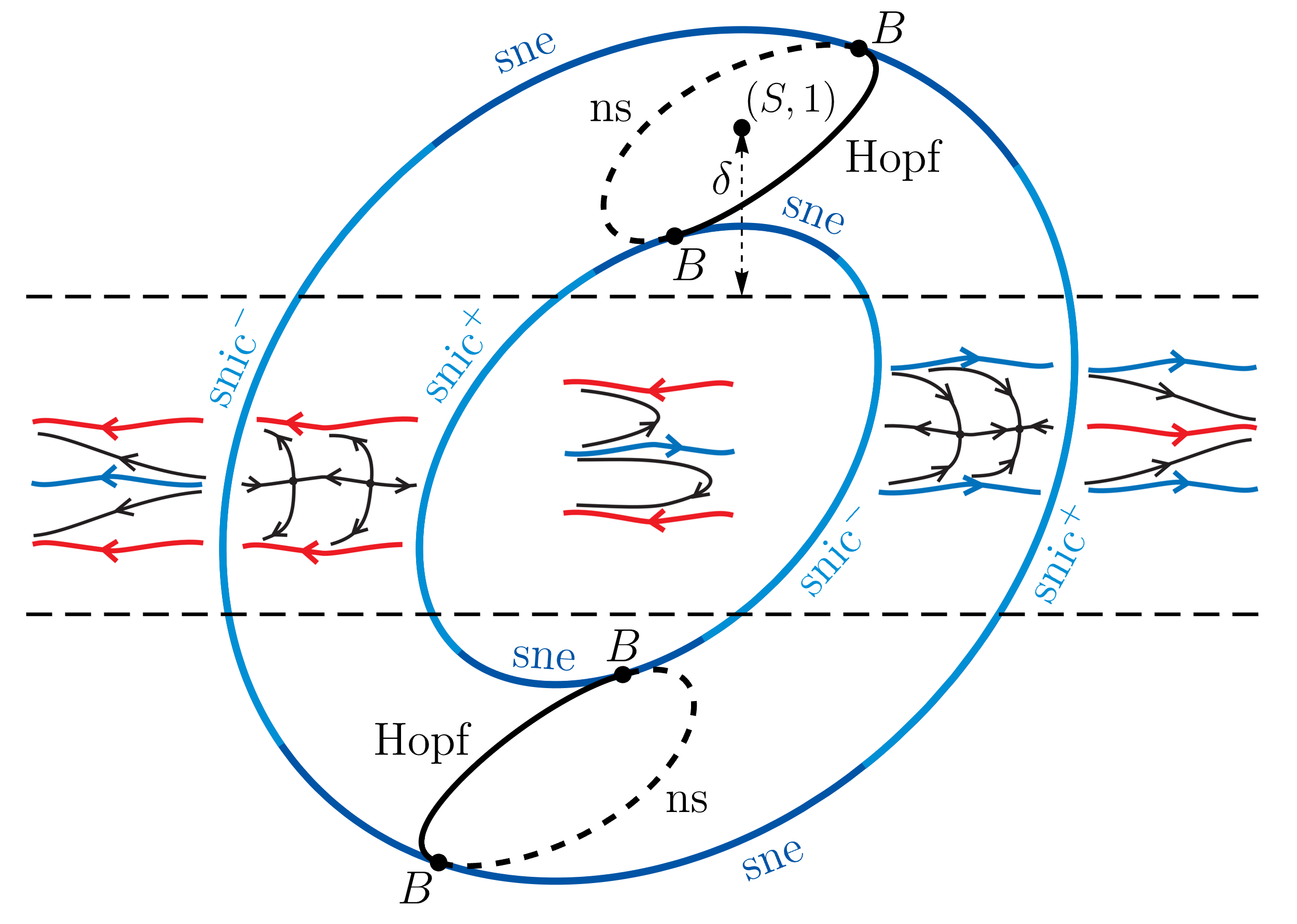
Figure 3. Phase portraits in the five regions of parameter space into which the snic curves divide the strip $|\Omega_{y}|<1-\delta$. Attractive periodic orbits are depicted in red and repelling ones in blue. The signs $\pm$ indicate that the periodic orbit created by snic is right-going/left-going. The transitions to snic along the curves of sne require $Z$ points that are not depicted here.

If in $\Omega_{x}\geq 0$ we move our parameters from the hole to the outside of $\mathcal{R}$, we see that the attracting periodic orbit experiences a saddle-node on an invariant circle (snic) bifurcation on entering the resonance region, then the equilibria do roughly half a revolution in opposite directions, meeting and experiencing another snic bifurcation when leaving the resonance region, see figure 3. We have the same behaviour for the repelling circle in $\Omega_{x}\leq 0$.

To make the transition along the sne curves from the $B$ points to the arcs of snic, there must be a $Z$ point, whose study is deferred to the next section.

2.5. First look at flow in $|\Omega_{y}\mp 1|\leq\delta$ and $|\Omega_{x}\mp S|\leq\sqrt{3\delta}$

We now consider all parameter values not studied in the previous sections that are close to the resonance region. Thus, we are interested in finding where the resonance region intersects the bands $|\Omega_{y}\mp 1|\leq\delta$. Using that the resonance region is an $\varepsilon$-neighbourhood of the ellipse $\psi$ we find that

$$|\Omega_{x}\mp S|\leq C\sqrt{2\delta(1+1/K)}+O(\varepsilon),$$

so for $\varepsilon$ small enough and $K>2$ we have $|\Omega_{x}\mp S|\leq\sqrt{3\delta}$. The factor 3 is missing in [BM18] owing to an oversight. Without loss of generality, from now on we will study the top of the resonance region, i.e. $|\Omega_{y}-1|\leq\delta$ and $|\Omega_{x}-S|\leq\sqrt{3\delta}$, which we denote by $\mathcal{Q}$.

Inspired by (2.3) we consider the parametrization,

$$\Omega=\psi(\theta)+\varepsilon\rho N_{\psi}(\theta),$$ (2.7)

so the resonance region is $|\rho|\leq 1$. Writing

$$\theta=\frac{1}{4}-\sqrt{\varepsilon}\,\alpha,$$

one finds on Taylor expanding (2.7) that

$$\begin{split}\Omega_{x}&=S+2\pi\sqrt{\varepsilon}C\alpha-2\pi^{2}\varepsilon S\alpha^{2}+O(\varepsilon^{\frac{3}{2}})\\ \Omega_{y}&=1+\varepsilon(\rho-2\pi^{2}\alpha^{2})+O(\varepsilon^{2})\end{split}$$ (2.8)

so in $\mathcal{Q}$ we have $\rho,\alpha=O(1)$. Now as $\Omega_{y}=1+O(\varepsilon)$, outside a neighbourhood of order $\sqrt{\varepsilon}$ of $y=\frac{1}{4}$, $\dot{y}>0$, and the flow eventually reaches this neighbourhood. Thus it is enough to study the flow in the regime $y=\frac{1}{4}+O(\sqrt{\varepsilon})$ which we do by writing

$$y=\frac{1}{4}+\sqrt{\varepsilon}\,\eta,$$

and as in this region the motion is slow we take $s=\sqrt{\varepsilon}\,t$ and use $\overset{\,\begin{picture}(-1.0,0.0)(-1.0,-1.0)\circle*{2.0}\end{picture}\ }{\vphantom{a}}$ for $\frac{\textnormal{d}}{\textnormal{d}s}$. Then, Taylor expanding (# ‣ 1.3) in these coordinates we get,

$$\overset{\,\begin{picture}(-1.0,0.0)(-1.0,-1.0)\circle*{2.0}\end{picture}\ }{x} =2\pi C(\eta+\alpha)+\sqrt{\varepsilon}\left(2\pi^{2}S(\eta^{2}-\alpha^{2})-\cos 2\pi x\right)+O(\varepsilon)$$ (2.9a)

$$\overset{\,\begin{picture}(-1.0,0.0)(-1.0,-1.0)\circle*{2.0}\end{picture}\ }{\eta} =2\pi^{2}(\eta^{2}-\alpha^{2})+\rho-\sin 2\pi x+O(\varepsilon).$$ (2.9b)

In [BM18, Section 2.7] it was shown that the study of the first order approximation of (2.9) leads to the following conclusions.

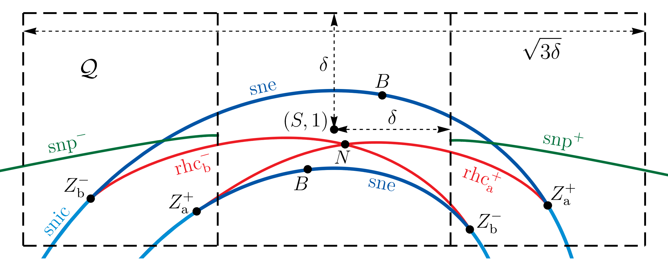
Figure 4. Sketch of the bifurcations diagram found so far in the top of the resonance region, $\mathcal{Q}$, excluding the trace-zero curves. We also depict the $\delta$-neighbourhood of $\bm{\mathbf{\Omega}}=(S,1)$ in dashed lines. The sign $\pm$ indicates right-going/left-going and a/b indicates that the homoclinic connection is above/below the saddle.

• For parameter values in the intersection of $\mathcal{Q}$ and the hole, the flow consists of precisely two Reeb components. Putting this together with the bottom of the resonance and section 2.4 we conclude that our example satisfies assumptions 4a and 4b.

• In the top of the resonance region there are precisely two curves where the vector field has a generic horizontal rotational homoclinic connection (rhc). Moreover, these curves are given by smooth graphs $\alpha^{\pm}(\rho)$. There are no other horizontal rhc curves, besides the analogous ones in the bottom of $\mathcal{R}$ so assumption 5c is satisfied. The two rhc curves from the top of the resonance region intersect at $\alpha=O(\sqrt{\varepsilon})$ forming an $N$ point, i.e. a saddle with two rhc. Uniqueness of this intersection will be deduced in section 3.2.

• Each horizontal rhc curve meets each boundary curve of $\mathcal{R}$ once where we have a generic $Z$ point, i.e. a saddle-node with a rhc between the neutral direction and the hyperbolic one. So we have precisely four $Z$ points of horizontal homotopy type on each component of the boundary of $\mathcal{R}$, thus justifying assumption 5.̱ It also justifies assumption 5a, as in the inner boundary we have horizontal homotopy type.

• Assuming genericity, we can deduce that in the band $|\rho-2\pi^{2}\alpha^{2}|<1$ and to the right (resp. left) of a $\delta$-neighbourhood of $\bm{\mathbf{\Omega}}=(S,1)$ (in the maximum norm), we have a curve of horizontal rotational saddle-node periodic orbits (snp) above the corresponding rhc curve, see figure 3. The snp could possibly have cusps and self-intersections, though they would imply regions with more than two horizontal periodic orbits. We did not rule this out but consider it unlikely; moreover it does not directly affect any of the properties we want our system to satisfy.

2.5.1. Lack of chc and cpo outside a $\delta$-neighbourhood of $\bm{\mathbf{\Omega}}=(S,1)$ while in $\mathcal{Q}$.

In the forthcoming section 3 we will narrow our attention to a $\delta$-neighbourhood of $\bm{\mathbf{\Omega}}=(S,1)$ in the maximum norm, see figure 3. So here we show that in $\mathcal{Q}$ but outside a $\delta$-neighbourhood of $\bm{\mathbf{\Omega}}=(S,1)$, there is no parameter value with a contractible homoclinic connection (chc) nor a contractible periodic orbit (cpo). Using (2.8) we find that in this region $|\alpha|>\sqrt{\varepsilon}\frac{K}{2\pi C}+O(\varepsilon)$ and as cpo and chc require equilibria, we can restrict our attention to $|\rho|\leq 1$.

First note that the divergence of (2.9) (i.e. trace of the derivative of the vector field) is

$$\operatorname{tr}=4\pi^{2}\eta+2\pi\sqrt{\varepsilon}\sin 2\pi x+O(\varepsilon).$$ (2.10)

From (2.9a) we find that the equilibria are located at $\eta=-\alpha+\sqrt{\varepsilon}\frac{\cos 2\pi x}{2\pi C}+O(\varepsilon)$ so that the trace at them is

$$\operatorname{tr}=-4\pi^{2}\alpha+2\pi\sqrt{\varepsilon}\left(\sin 2\pi x+C^{-1}\cos 2\pi x\right)+O(\varepsilon)$$

The sign of this expression is then dominated by the first term if $K>2(C+1)$ as $|\alpha|>\sqrt{\varepsilon}\frac{K}{4\pi C}$ for $\varepsilon$ small enough.

Now a cpo, $\gamma$, with period $T$ would have Lyapunov exponent $\frac{1}{T}\int_{\gamma}\operatorname{tr}\textnormal{d}s$ which from (2.10) and (2.9a) can be written as,

$$-4\pi^{2}\alpha+\frac{2\pi}{C}\sqrt{\varepsilon}\int_{\gamma}\frac{1}{T}\biggl{(}\frac{\overset{\,\begin{picture}(-1.0,0.0)(-1.0,-1.0)\circle*{2.0}\end{picture}\ }{x}}{\sqrt{\varepsilon}}-2\pi^{2}S(\eta^{2}-\alpha^{2})+\cos 2\pi x+C\sin 2\pi x\biggr{)}\,\textnormal{d}s+O(\varepsilon).$$ (2.11)

Again we want to show that the sign of the Lyapunov exponent is dominated by the first term, so we focus on bounding the integral. To this end we note that the $\overset{\,\begin{picture}(-1.0,0.0)(-1.0,-1.0)\circle*{2.0}\end{picture}\ }{\eta}$-nullclines are contained in

$$2\pi^{2}|\eta^{2}-\alpha^{2}|<|\rho|+1+O(\varepsilon),$$ (2.12)

so outside these horizontal bands $\eta$ is strictly monotonic and thus cpos must be contained in (2.12). Moreover, as $\gamma$ is contractible, $\int_{\gamma}\overset{\,\begin{picture}(-1.0,0.0)(-1.0,-1.0)\circle*{2.0}\end{picture}\ }{x}\,\textnormal{d}s=0$ so that the integral in (2.11) is bounded above by

$$\frac{1}{T}\int_{\gamma}S(|\rho|+1)+|\cos 2\pi x|+C|\sin 2\pi x|\,\textnormal{d}s+O(\varepsilon),$$

and hence also by $2S+C+1$. Recall that $|\alpha|>\sqrt{\varepsilon}\frac{K}{4\pi C}$ so that if $K>2(2S+C+1)$, the sign of the Lyapunov exponent is given by the first term in (2.11).

In conclusion, the sign of the Lyapunov exponent coincides with the sign of the trace at the equilibria. We can deduce then that there cannot exist cpos in this regime, as they would have the same attracting/repelling nature as the node and would give rise to impossible phase portraits. Essentially the same argument shows that there are no chc either.

3. $\delta$-neighbourhood of top and bottom of resonance region

To complete our analysis of the vector field, we zoom in on the $\delta$-neighbourhood of $\bm{\mathbf{\Omega}}=(S,1)$ in the maximum norm as depicted in figure 3(similar analysis can be done for $\bm{\mathbf{\Omega}}=(-S,-1)$). Here, we derive an approximation for the vector field which is reversible (conjugate to its time-reverse) and symplectic (locally Hamiltonian). We use the remainder terms to prove that for small $\varepsilon$ there is a unique $N$ point which is connected to the $B$ points by arcs of chc. We will also use these remainder terms in the upcoming section 4 and 5 to show that there are precisely two $K$ points and a unique $H$ point, and give numerical evidence that there is at most one cpo.

3.1. Reversible approximation

To study a $\delta$-neighbourhood of $\Omega=(S,1)$ we specialize the approximation in (2.9) by letting $\alpha=\sqrt{\varepsilon}\,\tilde{\alpha}/(2\pi)$, so

$$\begin{split}\overset{\,\begin{picture}(-1.0,0.0)(-1.0,-1.0)\circle*{2.0}\end{picture}\ }{x}&=2\pi C\eta+\sqrt{\varepsilon}\,(C\tilde{\alpha}-\cos 2\pi x+2\pi^{2}S\eta^{2})+O(\varepsilon)\\ \overset{\,\begin{picture}(-1.0,0.0)(-1.0,-1.0)\circle*{2.0}\end{picture}\ }{\eta}&=\rho-\sin 2\pi x+2\pi^{2}\eta^{2}+O(\varepsilon).\end{split}$$ (3.1)

In this section we study the unperturbed case $\varepsilon=0$,

$$\begin{split}\overset{\,\begin{picture}(-1.0,0.0)(-1.0,-1.0)\circle*{2.0}\end{picture}\ }{x}&=2\pi C\eta\\ \overset{\,\begin{picture}(-1.0,0.0)(-1.0,-1.0)\circle*{2.0}\end{picture}\ }{\eta}&=\rho-\sin 2\pi x+2\pi^{2}\eta^{2}\end{split}$$ (3.2)

which is a family of reversible vector fields with respect to the reflection $\eta\rightarrow-\eta$ and we denote it by $\mathbf{v}_{\rho}$. Inspired by [BM18, Section 2.8.1], we find that on the universal cover they are Hamiltonian with respect to the symplectic form,

$$\mathcal{A}=e^{-2\pi x/C}\textnormal{d}x\wedge\textnormal{d}\eta.$$

Indeed, we have

$$e^{-2\pi x/C}\,\overset{\,\begin{picture}(-1.0,0.0)(-1.0,-1.0)\circle*{2.0}\end{picture}\ }{x}=H_{\eta},\hskip 45.52458pte^{-2\pi x/C}\,\overset{\,\begin{picture}(-1.0,0.0)(-1.0,-1.0)\circle*{2.0}\end{picture}\ }{\eta}=-H_{x},$$

where the Hamiltonian is

$$H(x,\eta)=e^{-2\pi x/C}\left(\pi C\eta^{2}+\frac{C\rho}{2\pi}-\frac{1}{4\pi}g(x)\right),$$

with

$$g(x)=\frac{2C}{1+C^{2}}\left(C\cos 2\pi x+\sin 2\pi x\right),$$ (3.3)

which is found by solving the relation $\frac{1}{2C}g(x)-\frac{1}{4\pi}g^{\prime}(x)=\sin 2\pi x$. Because $C>0$, this can be rewritten as

$$g(x)=\frac{2C}{\sqrt{1+C^{2}}}\cos 2\pi(x-x_{g})$$

with $x_{g}=\frac{1}{2\pi}\arctan\frac{1}{C}$, where we take the standard determination of arctangent from $-\frac{\pi}{2}$ to $\frac{\pi}{2}$.

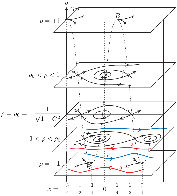
Figure 5. Sketch of the phase portraits for the reversible family of vector fields (3.2) at selected values of $\rho$. To increase visibility, the $\rho$-axis and the phase portraits have been slightly distorted.

We now study the phase portraits using the fact that $H$ is conserved along trajectories. They have two distinct regimes separated by a parameter value $\rho_{0}$ with a necklace as depicted in figure 5. To compute $\rho_{0}$ we first note that as our phase space is a cylinder $\mathbb{T}^{1}\times\mathbb{R}$ any rotational homoclinic connection or periodic orbit will be invariant under $x\mapsto x+1$. As $H$ has a non-periodic factor, the only invariant level set under $x\mapsto x+1$ is $H=0$.

The equilibrium points of the system are at $\eta=0$ and $\sin 2\pi x=\rho$, where $\det=4\pi^{2}\cos 2\pi x$, so the saddle is at $x_{\operatorname{sad}}\in(\frac{1}{4},\frac{3}{4})$ mod 1 and the centre at $x_{\operatorname{cen}}\in(-\frac{1}{4},\frac{1}{4})$ mod 1. The rhc occurs when the energy at the saddle, $E_{\operatorname{sad}}=H(x_{\operatorname{sad}},0)$, vanishes, i.e.

$$\frac{C\rho_{0}}{2\pi}=\frac{g(x_{\operatorname{sad}})}{4\pi}\quad\Longleftrightarrow\quad\rho_{0}=\frac{1}{1+C^{2}}\left(-C\sqrt{1-\rho_{0}^{2}}+\rho_{0}\right)$$

and with some algebra we get $\rho_{0}=-1/\sqrt{1+C^{2}}$. The rhc are then given by the level set $H=0$ at $\rho_{0}$ so

$$\eta=\pm\sqrt{\frac{\cos 2\pi(x-x_{g})+1}{2\pi^{2}\sqrt{1+C^{2}}}}=\pm\frac{1}{\pi\sqrt[4]{1+C^{2}}}\cos\pi(x-x_{g}).$$ (3.4)

For $\rho\in(-1,\rho_{0})$, $E_{\operatorname{sad}}<0$, so its level set includes a contractible homoclinic loop to the right of the saddle, whereas for $\rho\in(\rho_{0},1)$, $E_{\operatorname{sad}}>0$, so it has a contractible homoclinic loop to the left. Each contractible homoclinic loop bounds a region foliated by cpos around a centre, see figure 5.

Note that, despite its Hamiltonian nature on the universal cover, the vector field can have attracting and repelling rotational periodic orbits. Indeed, the level set $H=0$ gives explicitly

$$2\pi\eta=\pm\sqrt{g(x)/C-2\rho}$$ (3.5)

which for $\rho<\rho_{0}$ gives two rotational periodic orbits, see figure 5. Integrating the divergence of (3.2) by changing integration variable to $x$ we find that they have Floquet multipliers $e^{\pm 2\pi/C}$ respectively. The square of (3.5) also gives a periodic orbit for $\rho\in(\rho_{0},1)$ but it is just one of a continuum of contractible and neutrally stable ones inside the chc.

In the following sections we use Pontryagin’s energy balance method, see [Pon34] and [BM18, Section 2.8.2], to determine where various features of the reversible approximation persist on adding the correction terms. In this method we consider $\gamma$ a closed orbit of the unperturbed system $\mathbf{v}_{\rho}$. Then, the increment of $H$ for nearby orbits in the perturbed vector field $\mathbf{v}_{\rho}+\sqrt{\varepsilon}\tilde{\mathbf{v}}+O(\varepsilon)$ is,

$$\Delta H=\int_{\gamma}\overset{\,\begin{picture}(-1.0,0.0)(-1.0,-1.0)\circle*{2.0}\end{picture}\ }{H}\,\textnormal{d}s+O(\varepsilon)=\sqrt{\varepsilon}\left(\int_{\gamma}e^{-2\pi x/C}\tilde{v}_{2}\,\textnormal{d}x-\int_{\gamma}e^{-2\pi x/C}\tilde{v}_{1}\,\textnormal{d}\eta\right)+O(\varepsilon).$$ (3.6)

so that the closed orbit persists only when $\Delta H=0$. Moreover, if the coefficient of $\sqrt{\varepsilon}$ in (3.6) has a non-degenerate zero (or submanifold of non-degenerate zeroes) as a function of parameters, then the orbit only survives along a submanifold in parameter space $\mathcal{C}^{1}$-close to where the first term vanishes.

3.2. Rotational homoclinic connection (rhc) and necklace point ($N$)

First, we compute where the unperturbed $\textrm{rhc}^{\pm}$ given by (3.4) persist, by letting $\rho=\rho_{0}+\sqrt{\varepsilon}\,\tilde{\rho}$. So the vector field is $\mathbf{v}_{\rho_{0}}+\sqrt{\varepsilon}\tilde{\mathbf{v}}+O(\varepsilon)$ with

$$\tilde{\mathbf{v}}=(C\tilde{\alpha}-\cos 2\pi x+2\pi^{2}S\eta^{2},\tilde{\rho}).$$

If we denote by $\gamma_{\pm}$ the unperturbed $\textrm{rhc}^{\pm}$ from $x_{g}-1/2$ to $x_{g}+1/2$, we see from (3.6) that they persist along

$$\Delta H=\sqrt{\varepsilon}\,(c\tilde{\rho}-Ca\tilde{\alpha}+b)+O(\varepsilon)=0$$

where,

$$a =\int_{\gamma_{+}}e^{-2\pi x/C}\,\textnormal{d}\eta=-\int_{\gamma_{+}}e^{-2\pi x/C}\frac{\sin\pi(x-x_{g})}{\sqrt[4]{1+C^{2}}}\,\textnormal{d}x=\frac{4Ce^{-C^{-1}\arctan{\frac{1}{C}}}\cosh{\frac{\pi}{C}}}{\pi\sqrt[4]{1+C^{2}}\,(4+C^{2})},$$

$$b =\int_{\gamma_{+}}e^{-2\pi x/C}(\cos 2\pi x-2\pi^{2}S\eta^{2})\,\textnormal{d}\eta$$

$$=-\int_{\gamma_{+}}e^{-2\pi x/C}\left(\cos 2\pi x-2S\frac{\cos^{2}\pi(x-x_{g})}{\sqrt{1+C^{2}}}\right)\frac{\sin\pi(x-x_{g})}{\sqrt[4]{1+C^{2}}}\textnormal{d}x$$

$$=-a\frac{2C^{2}(C+2S)}{\sqrt{1+C^{2}}\,(4+9C^{2})},$$

$$c =\int_{\gamma_{+}}e^{-2\pi x/C}\,\textnormal{d}x=a\frac{1}{4}\sqrt[4]{1+C^{2}}(4+C^{2})\,\tanh\frac{\pi}{C}>0.$$

For $\phi=0$ we recover the coefficients computed in the corrigendum [BLM22]. Then, by Pontryagin’s method the curves of $\textrm{rhc}^{\pm}$ are given to leading order in $\sqrt{\varepsilon}$ by

$$\tilde{\rho}=\pm(Ca\tilde{\alpha}-b)/c,$$ (3.7)

and are in fact $\mathcal{C}^{1}$-close to (3.7). The approximate curves $\textrm{rhc}^{\pm}$ cross transversely at $\tilde{\rho}=0$ and

$$\tilde{\alpha}=\frac{b}{Ca}=-\frac{2C(C+2S)}{\sqrt{1+C^{2}}\,(4+9C^{2})},$$ (3.8)

forming a generic $N$ point (non-vanishing trace will be shown below).

There is no other horizontal rhc in $|\rho|\leq 1$, $\tilde{\alpha}=O(1)$, because the phase portraits for the reversible approximation allow such a feature only near $\rho=\rho_{0}$, where Pontryagin’s method above gives the locally unique curves found. So the $N$ point found above is unique in this region of parameters, which by section 2.5 is the only possible location of an $N$ point in the top of the resonance region. Doing the same for the bottom we prove assumption 6.

In addition to the two curves of rhc the unfolding of a necklace point contains two arcs of chc whose direction is determined by the sign of the trace at the saddle [BGKM91]. From (2.6) and (2.8) we deduce that the trace-zero loop in $(\tilde{\alpha},\rho)$ parameters is $\mathcal{C}^{1}$-close to the ellipse

$$\rho^{2}+C^{2}(\tilde{\alpha}-\rho)^{2}=1.$$ (3.9)

Thus substituting (3.8) and $\rho_{0}$ we see that the $N$ point is inside the trace-zero loop. In particular it is to the right of the ns curve, so the trace at the saddle is negative. Hence, the chc emanate to the right of the necklace point as depicted in figure 6. Note that, as mentioned in the corrigendum [BLM22], in the case $\phi=0$ we also get the $N$ point inside the trace-zero loop.

3.3. Contractible homoclinic connection (chc)

Next we compute how the contractible homoclinic connections of the reversible approximation, $\gamma$, persist for each $\rho\in(-1,\rho_{0})\cup(\rho_{0},1)$. We apply Pontryagin’s method, where the coefficient in (3.6) vanishes if

$$Ca(\rho)\tilde{\alpha}-b(\rho)=0$$

where

$$a(\rho)=\int_{\gamma}e^{-2\pi x/C}\,\textnormal{d}\eta,\hskip 42.67912ptb(\rho)=\int_{\gamma}e^{-2\pi x/C}(\cos 2\pi x-2\pi^{2}S\eta^{2})\,\textnormal{d}\eta.$$

So for each $\rho$ there is a unique $\tilde{\alpha}$ with chc, close to $\tilde{\alpha}(\rho)=C^{-1}b(\rho)/a(\rho)$, since $a(\rho)>0$, as we proceed to show. First note that if we change variables to $x$ and then integrate by parts while using that $\gamma$ is contractible we get

$$\int_{\gamma}e^{-2\pi x/C}h(x)\,\textnormal{d}\eta=\int_{\gamma}\left(\tfrac{2\pi}{C}h(x)-h^{\prime}(x)\right)e^{-2\pi x/C}\eta\,\textnormal{d}x$$

for any function $h$. Picking $h=1$, we obtain,

$$a(\rho)=\frac{2\pi}{C}\int_{\gamma}e^{-2\pi x/C}\eta\,\textnormal{d}x=\frac{2\pi}{C}\int_{\bar{\gamma}}e^{-2\pi x/C}\,\textnormal{d}x\,\textnormal{d}\eta>0,$$ (3.10)

where $\bar{\gamma}$ denotes the region bounded by the chc $\gamma$. For $b(\rho)$ we let $h(x)=\cos 2\pi x-2\pi\frac{S}{C}(\pi C\eta^{2})$, and note that the level set of the chc is $\pi C\eta^{2}=e^{2\pi x/C}E_{\operatorname{sad}}-\frac{C\rho}{2\pi}+\frac{g(x)}{4\pi}$. Then some algebra, that can be simplified using the relation below (3.3), gives

$$b(\rho)=\frac{2\pi}{C}\int_{\gamma}(f(x)+S\rho)e^{-2\pi x/C}\eta\,\textnormal{d}x=\frac{2\pi}{C}\int_{\bar{\gamma}}(f(x)+S\rho)e^{-2\pi x/C}\,\textnormal{d}x\,\textnormal{d}\eta,$$ (3.11)

where

$$f(x)=\cos 2\pi x+(C-S)\sin 2\pi x.$$ (3.12)

The chc tends to the concatenation of the two rhcs as $\rho\rightarrow\rho_{0}$ thus $C^{-1}b(\rho)/a(\rho)\rightarrow C^{-1}b/a$ from (3.8), i.e. the chc curves tend to the approximate location of the necklace as $\rho\rightarrow\rho_{0}$, which is consistent with the unfolding of the $N$ point.

Figure 6. Bifurcation diagram for (3.1) in $(\tilde{\alpha},\rho)$ excluding the intersections of the rhc curves with ns and their consequences. The rhc curves are horizontal to first order but for clarity they and the chc curves are not drawn to scale. Parameter values in the orange shaded region have a cpo as will be shown in the following section.

Note that $\tilde{\alpha}=C^{-1}b(\rho)/a(\rho)$, can be interpreted as the average value of $(f+S\rho)/C$, in the region $\bar{\gamma}$, weighted by $e^{-2\pi x/C}$. When $\rho\rightarrow\pm 1$ the chc shrinks to a point so $\tilde{\alpha}$ tends to the value of $(f+S\rho)/C$ at the saddle. Thus, using $\sin 2\pi x_{\operatorname{sad}}=\rho$, we find $\tilde{\alpha}\rightarrow\pm 1$ when $\rho\rightarrow\pm 1$. These are also the approximate locations of the $B$ points, which can be deduced from (3.9) and the fact that on the boundary of the resonance $\rho=\pm 1$. Using the genericity of the $N$ and $B$ points we can conclude that the chc curves connect the $B$ points to the $N$ point as depicted in figure 6.

Finally, we prove that the curves of chc do not intersect that of ns, so there is no $J$ point, justifying assumption 7a and the genericity of the curves of chc. Using $\sin 2\pi x_{\operatorname{sad}}=\rho$ and (3.9), we find that the curve of ns has

$$\tilde{\alpha}\sim\frac{\cos 2\pi x_{\operatorname{sad}}+C\sin 2\pi x_{\operatorname{sad}}}{C}=\frac{f(x_{\operatorname{sad}})+S\rho}{C}.$$

Thus, proving $\tilde{\alpha}_{\textrm{chc}}>\tilde{\alpha}_{\textrm{ns}}$ is equivalent to showing that the average of $f$ over the region bounded by the chc (weighted by $e^{-2\pi x/C}$) is bigger than $f(x_{\operatorname{sad}})$, since the constant terms cancel out. Showing this is tedious and not particularly insightful when $\phi\not=0$, but can be done; see appendix D.

4. Contractible periodic orbits

In this section we show numerically that the cpos of the reversible approximation give rise to a unique cpo for each parameter value in the zone between the curves of chc and the Hopf curve, i.e. the shaded orange region in figure 6. Our analysis also shows that no cpo persist for parameters outside this region. Moreover, the phase diagram of the reversible approximation does not allow for the appearance of any other cpo. In particular, there is at most one cpo for parameter values in a $\delta$-neighbourhood of the top or bottom of the resonance region. Outside these neighbourhoods we have shown in section 2.4 and 2.5.1 that there are no cpos, so we can conclude that assumption 7b is satisfied.

We note that when applying Pontryagin’s method in section 3.3 we never used that the specific level curve contained the saddle, nor its specific energy $E_{\operatorname{sad}}$. So exactly the same arguments show that a cpo $\gamma$ with energy $E$ persists at parameter value $\rho$ for a unique $\tilde{\alpha}$ given to first order by $\tilde{\alpha}(E,\rho)=C^{-1}b(E,\rho)/a(E,\rho)$, where from (3.10) and (3.11) we get

$$\begin{split}a(E,\rho)&=\frac{4\pi}{C}\int_{x_{\min}}^{x_{\max}}e^{-2\pi x/C}\eta(x)\,\textnormal{d}x,\\ b(E,\rho)&=\frac{4\pi}{C}\int_{x_{\min}}^{x_{\max}}(f(x)+S\rho)e^{-2\pi x/C}\eta(x)\,\textnormal{d}x,\end{split}$$

with $x_{\min}$, $x_{\max}$ the intersections of $\gamma$ with the $x$-axis, and $\eta(x)$ the part of $\gamma$ above it. If we denote by $E_{\operatorname{cen}}$ the energy at the centre inside the cpo and by $E_{\operatorname{sad}}$ the energy at the saddle on the chc enclosing the cpo, we have $E_{\operatorname{cen}}\leq E_{\operatorname{sad}}$ and $E\in(E_{\operatorname{cen}},E_{\operatorname{sad}})$. When $E\rightarrow E_{\operatorname{sad}}$, the cpo tends to the chc, so we get $\tilde{\alpha}(E,\rho)\rightarrow\tilde{\alpha}(\rho)$ from section 3.3, the approximate value of $\tilde{\alpha}$ at the chc curves. Note that, as in the case of chc, $\tilde{\alpha}(E,\rho)$ can be interpreted as the average of the function $(f+S\rho)/C$ (weighted by $e^{-2\pi x/C}$) in the region bounded by the cpo. So when $E\rightarrow E_{\operatorname{cen}}$ and the cpo shrinks to a point, $\tilde{\alpha}(E,\rho)$ tends to the value of the function at the centre. Using that $\sin 2\pi x_{\operatorname{cen}}=\rho$ we find that as $E\rightarrow E_{\operatorname{cen}}$,

$$\tilde{\alpha}(E,\rho)\rightarrow\rho+C^{-1}\sqrt{1-\rho^{2}},$$

which from (3.9), is the approximate value of $\tilde{\alpha}$ at the Hopf curve.

Now if we show that for a fixed $\rho\in(-1,1)$, $\tilde{\alpha}(E,\rho)$ is strictly decreasing in the interval $(E_{\operatorname{cen}},E_{\operatorname{sad}})$, then we can conclude that for each parameter in the region between the chc curve and the Hopf curve, we have exactly one cpo.

To show that $\tilde{\alpha}(E,\rho)$ is decreasing on $E$, we compute its derivative,

$$\tilde{\alpha}^{\prime}(E,\rho):=\frac{\partial\tilde{\alpha}}{\partial E}(E,\rho)=\frac{b^{\prime}a-ba^{\prime}}{Ca^{2}}$$ (4.1)

where everything on the right is evaluated at $(E,\rho)$, and

$$\begin{split}a^{\prime}(E,\rho)&:=\frac{\partial a}{\partial E}(E,\rho)=\frac{2}{C^{2}}\int_{x_{\min}}^{x_{\max}}\frac{1}{\eta(x)}\,\textnormal{d}x,\\ b^{\prime}(E,\rho)&:=\frac{\partial b}{\partial E}(E,\rho)=\frac{2}{C^{2}}\int_{x_{\min}}^{x_{\max}}\frac{f(x)+S\rho}{\eta(x)}\,\textnormal{d}x,\end{split}$$

which have been computed by differentiating under the integral sign, while using that $\eta(x_{\min})=\eta(x_{\max})=0$. When computing (4.1) one can remove the $S\rho$ term in $b$ and $b^{\prime}$ using that $\tilde{\alpha}^{\prime}=(\tilde{\alpha}-S\rho)^{\prime}$.

As we are not able to compute the integrals, nor derive useful bounds on (4.1), we check the sign of $\tilde{\alpha}^{\prime}$ numerically.

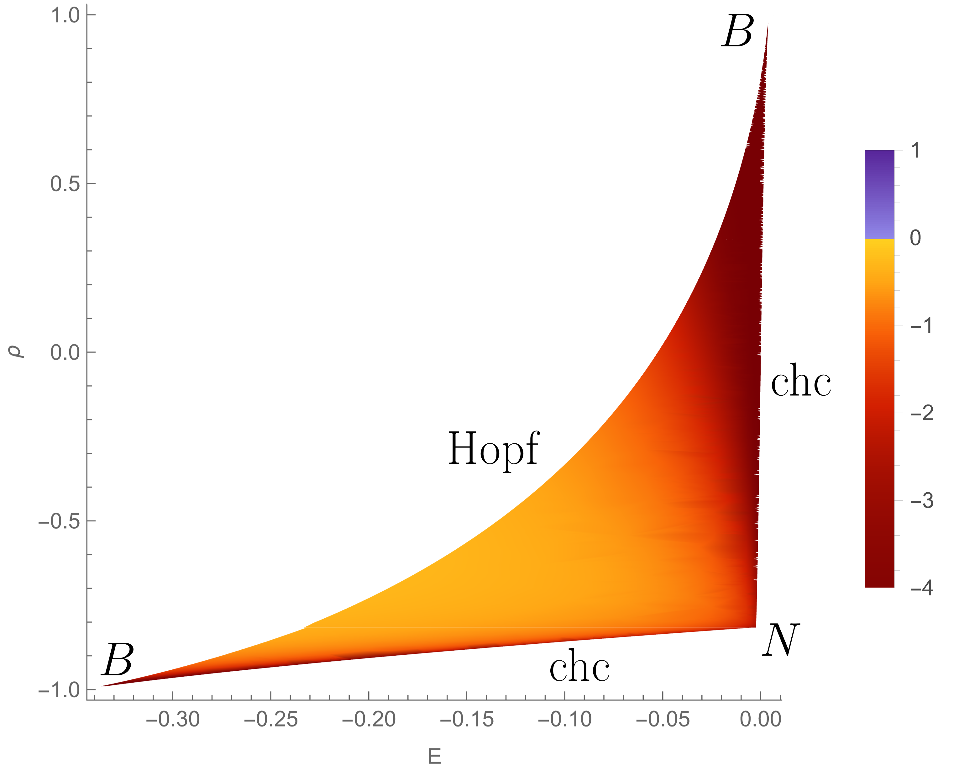
Figure 7. Density plot of $\tilde{\alpha}^{\prime}$ in the regime of interest with $\phi=1/8$. There is no parameter value shaded with positive colour. Note that this region corresponds to the orange shaded region in figure 6. Note also that the righthand boundary in this figure is not quite vertical.

To present the numerical computations we chose $\phi=\frac{1}{8}$, which is enough to make an example of the simplest bifurcation diagram. We note though, that we have not seen significant difference with other values $\phi\in(\frac{1}{24},\frac{5}{24})$. Figure 7 depicts a Mathematica density plot of $\tilde{\alpha}^{\prime}$ in the region bounded by the Hopf curve and the chc curves. As the density plot does not have blue regions, or even light yellows, we are fairly confident that the value of $\tilde{\alpha}^{\prime}$ is always negative and significantly away from zero. We can conclude then that $\tilde{\alpha}$ is decreasing on $E$.

To end this section we note that in the density plot it seems that $\tilde{\alpha}^{\prime}$ has singularities at the $B$ points; this is expected for generic $B$ points.

5. $K$ and $H$ points

Finally, we find the intersections of $\textrm{rhc}^{\pm}$ curves with the ns and the horizontal snp curves, which give rise to $K$ and $H$ points respectively.

Recall from (3.7) that the $\textrm{rhc}^{\pm}$ curves are $\mathcal{C}^{1}$-close to lines with steepness $\pm Ca/c$ in the $(\tilde{\alpha},\tilde{\rho})$ plane. In this plane $\rho\sim\rho_{0}$, so that from (3.9), we deduce that the ns curve has $\textnormal{d}\tilde{\alpha}/\textnormal{d}\rho\sim-S^{2}/C^{2}$. It must then be nearly vertical in the $(\tilde{\alpha},\tilde{\rho})$ plane, due to the $\sqrt{\varepsilon}$ scaling, and thus it intersects once with each rhc curve, see figure 8. This gives precisely two $K$ points, which are generic, as the intersections are transverse and the trace has non-zero derivative across the ns curve. Their location can be found by substituting $\rho\sim\rho_{0}$ in (3.9) and then using (3.7), which gives

$$\tilde{\alpha}\sim 2\rho_{0},\hskip 28.45274pt\tilde{\rho}\sim\mp\frac{16C(2-SC+4C^{2})}{(1+C^{2})^{3/4}(4+C^{2})(4+9C^{2})\tanh\frac{\pi}{C}}.$$

Putting together the top and the bottom of the resonance region proves assumption 8.

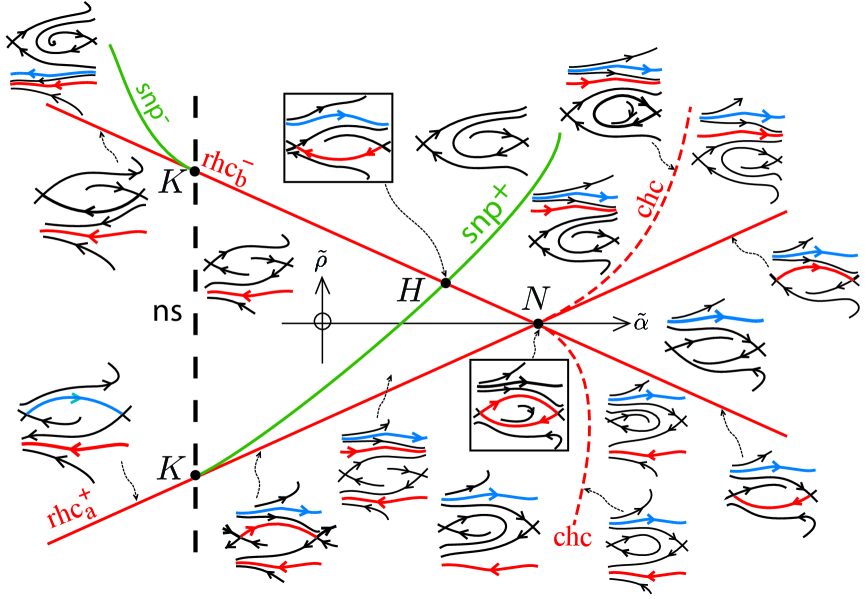
Figure 8. Bifurcation diagram in $(\tilde{\alpha},\tilde{\rho})$ coordinates around the $N$, $K$ and $H$ points leaving out the Hopf curve and the fan of rhc emanating from the $H$ point. The $\textnormal{snp}^{\pm}$ coincide to first order with the $\textnormal{rhc}^{\pm}$ curves but for clarity we have exaggerated their separation ($\pm$ indicates right-going/left-going).

Generically, a $K$ point produces an arc of generic snp, tangent to the curve of rhc at the $K$ point. For this example, they must occur in the directions shown in figure 8 for compatibility with the sign of trace at the saddle, the direction in which the rhcs break and the rotational periodic orbits that exist below the necklace and not above, as illustrated in the figure. The arcs of snp are $\mathcal{C}^{1}$-close to the corresponding rhc curves in the $(\tilde{\alpha},\tilde{\rho})$ plane, as we will show in the upcoming section. Thus, we have a unique intersection between snp and rhc curves of opposite direction, i.e. an $H$ point, which is close to the $N$ point as depicted in figure 8. Putting together the top and the bottom of the resonance region proves assumption 9.

Moreover, the $H$ point is generic as its intersection is transverse and the trace at the saddle is non-zero on it. In particular, we have tongues emanating from the top of $H$ with rhc curves as boundaries and unique rotational periodic orbits (attractive as the trace is negative) for parameter values in their interior [BM18]. In fact, there is a fan of tongues, one for each homology direction between $(\pm 1,0)$, where the homology direction of each tongue is given by the homotopy type and direction of its rotational periodic orbits. This has been omitted from figure 8, but it is depicted in figure 1, where it is also shown how some of these tongues may extend outside a neighbourhood of $H$.

5.1. Transit map

In this section we show that the snp curves are $\mathcal{C}^{1}$-close to the corresponding rhc curves in the $(\tilde{\alpha},\tilde{\rho})$ plane. In a neighbourhood of the $K$ points this follows from their genericity, see [Per94]. Outside this neighbourhood we use the transit map and without loss of generality we focus on the $\textrm{snp}^{+}$ case.

The saddle is near $x_{g}+\frac{1}{2}$ so it is natural to consider the transit map $\mathcal{T}$ from $x=x_{g}$ to $x=x_{g}+1$. This map will be defined for $\eta>\eta_{s}$, the value of $\eta$ on the stable manifold at $x_{g}$, and will be mapped to $\hat{\eta}>\eta_{u}$, the value on the unstable one at $x_{g}+1$. We will use the coordinate $z=\eta^{2}$ as $\eta_{s},\eta_{u}>0$ and it will simplify some formulae.

Using the Hamiltonian (3.1) with $\rho=\rho_{0}$ we find that in the unperturbed case, where we have a necklace point, the transit map is simply

$$\mathcal{T}(z)=e^{2\pi/C}(z-K),$$ (5.1)

with $K=(e^{-2\pi/C}-1)\rho_{0}/\pi^{2}>0$ and fixed point $z_{s}=z_{u}=-\rho_{0}/\pi^{2}>0$. In the perturbed case, $z_{u}=z_{s}$ iff there exists a $\textnormal{rhc}^{+}$. So the rhc is detected by

$$z_{u}-z_{s}=0$$ (5.2)

where by the stable manifold theorem $z_{u}$ and $z_{s}$ are smooth on parameters.

From (5.1) we note that the slope of the perturbed transit map is close to $e^{2\pi/C}>1$ for $z$ sufficiently above $z_{s}$, because the return time is bounded, so there is no snp there. Thus, it is left to study $\mathcal{T}^{\prime}(z)$ when $z$ is close to $z_{s}$, which we will quantify shortly, where the return time goes to infinity.

We will study $\mathcal{T}^{\prime}(z)$ by exploring the evolution of the symplectic area $\mathcal{A}=e^{-2\pi x/C}\textnormal{d}x\wedge\textnormal{d}\eta$. First consider the coordinate $\chi=-\frac{C}{2\pi}e^{-2\pi x/C}$ so that $\mathcal{A}$ is the standard area, i.e. $\mathcal{A}=\textnormal{d}\chi\wedge\textnormal{d}\eta$. Then, its rate of growth is given by the divergence of the vector field in these coordinates, that is $\overset{\hskip 2.8pt\,\begin{picture}(-1.0,0.0)(-1.0,-1.0)\circle*{2.0}\end{picture}\ }{\mathcal{A}}=\tau\mathcal{A}$, where

$$\tau=2\pi\sqrt{\varepsilon}\left(\sin 2\pi x-\tilde{\alpha}+\frac{1}{C}\cos 2\pi x-2\pi^{2}\frac{S}{C}\eta^{2}\right)+O(\varepsilon).$$ (5.3)

So if we consider the path $\gamma$ for the flow from $(x_{g},\eta)$ to $(x_{g}+1,\hat{\eta})$ we have

$$\hat{\mathcal{A}}=\mathcal{A}e^{\int_{\gamma}\tau\,\textnormal{d}s}.$$

Applying $\mathcal{A}$ to the vector field (3.1) and a vertical vector $\delta\eta$ at the initial point yields $e^{-2\pi x_{g}/C}(2\pi C\eta+O(\sqrt{\varepsilon}))\,\delta\eta$. During the transit, this area gets multiplied by $e^{\int_{\gamma}\tau\,ds}$. The vector field is carried to the vector field at the image point; the vertical vector is carried to a vector that in general is not vertical, but after adding a suitable multiple of the vector field it can be made a vertical vector $\delta\hat{\eta}$, spanning the same area. This pair spans area $e^{-2\pi(x_{g}+1)/C}(2\pi C\hat{\eta}+O(\sqrt{\varepsilon}))\,\delta\hat{\eta}$. So this yields

$$\mathcal{T}^{\prime}(z)=\frac{\delta(\hat{\eta}^{2})}{\delta(\eta^{2})}=e^{\int_{\gamma}\tau\,\textnormal{d}s}\left(e^{2\pi/C}+O(\sqrt{\varepsilon})\right),$$

as $\eta>\eta_{s}$, $\hat{\eta}>\eta_{s}$ and $\eta_{s},\eta_{u}\sim\sqrt{-\rho_{0}}/\pi>0$ which has been deduced from (5.1).

To compute the integral in the exponent consider a neighbourhood $U$ of the saddle where a smooth conjugacy flattens the stable and unstable manifolds to coincide with the axes. We can choose $U$ independent of $\varepsilon$ and such that $\gamma$ intersects the boundary transversely for $\eta$ close to $\eta_{s}$. Then, the time spent outside $U$ is bounded so the contribution of the integral there is $O(\sqrt{\varepsilon})$. The contribution in $U$ can be computed after flattening of the invariant manifolds as is done in appendix E. In total we get,

$$\int_{\gamma}\tau\,\textnormal{d}s=T\tau_{\operatorname{sad}}+O(\sqrt{\varepsilon})=T(\sqrt{\varepsilon}\,\tau_{0}+O(\varepsilon))+O(\sqrt{\varepsilon}),$$ (5.4)

where $T$ is the time spent in $U$ and in the second equality we approximate to first order $\tau$ at the saddle, $\tau_{\operatorname{sad}}$, by evaluating (5.3) at $(x_{g}+\frac{1}{2},0)$ so,

$$\tau_{0}=-2\pi\,(2\sin 2\pi x_{g}+\tilde{\alpha}).$$

If we let $\lambda$ be the unstable eigenvalue, $\lambda\sim 2\pi C(1+C^{2})^{-1/4}$, the time $T$ spent near the saddle is given by, $-\lambda^{-1}\log m(\eta-\eta_{s})$ where $m$ is around 1, that is, $m=O(1)$ and $1=O(m)$. Putting everything together,

$$\mathcal{T}^{\prime}(z)=\big{(}e^{2\pi/C}+O(\sqrt{\varepsilon})\big{)}\left(m(\eta-\eta_{s})\right)^{\sqrt{\varepsilon}\,\nu+O(\varepsilon)},$$ (5.5)

where $\nu=-\lambda^{-1}\tau_{0}>0$ and is around 1 as we are to the right of the neutral saddle curve (where the trace is zero) and outside a neighbourhood of the $K$ point. We are interested in points with slope 1, so that the second factor in (5.5) must be significantly smaller than one, in particular $\eta=\eta_{s}+O(\sqrt{\varepsilon})$. Thus,

$$z-z_{s}=(2\eta_{s}+O(\sqrt{\varepsilon}))(\eta-\eta_{s})$$

and converting to $z$ coordinates,

$$\mathcal{T}^{\prime}(z)=\left(e^{2\pi/C}+O(\sqrt{\varepsilon})\right)\left(\frac{z-z_{s}}{k+O(\sqrt{\varepsilon})}\right)^{\sqrt{\varepsilon}\,\nu+O(\varepsilon)},$$ (5.6)

where $k=2\eta_{s}/m$ and is around 1. Then, points with slope 1 are given by,

$$z-z_{s}=\left(k+O(\sqrt{\varepsilon})\right)\left(e^{-2\pi/C}+O(\sqrt{\varepsilon})\right)^{\frac{1}{\sqrt{\varepsilon}\hskip 1.0pt\nu+O(\varepsilon)}}.$$ (5.7)

We can compute the transit map by integrating $\mathcal{T}^{\prime}$ while using that $T(z_{s})=z_{u}$, so

$$\mathcal{T}(z)=z_{u}+\left(ke^{2\pi/C}+O(\sqrt{\varepsilon})\right)\left(\frac{z-z_{s}}{k+O(\sqrt{\varepsilon})}\right)^{1+O(\sqrt{\varepsilon})}.$$ (5.8)

We note that some error terms of $\mathcal{T}^{\prime}$ depend on $z$, so when we integrate treating them as constants we lose some control. In particular, one can check that all the errors in this section before (5.8) have derivatives with respect to parameters of the same order, whereas we cannot guarantee this for the terms in (5.8) which means we will have to be careful in our analysis.

Recall now that snp correspond to fixed points of $\mathcal{T}$ with slope 1, which by doing some algebra with (5.7) and (5.8) occur only when,

$$z_{u}-z_{s}=O(1)\left(e^{-2\pi/C}+O(\sqrt{\varepsilon})\right)^{\frac{1+O(\sqrt{\varepsilon})}{\sqrt{\varepsilon}\hskip 1.0pt\nu+O(\varepsilon)}}.$$ (5.9)

The right hand side of the expression above is exponentially small in $\sqrt{\varepsilon}$, so to all orders this equation is equivalent to (5.2), i.e. the $\textnormal{snp}^{+}$ is indistinguishable from the $\textnormal{rhc}^{+}$.

However, we cannot conclude that the $\textnormal{snp}^{+}$ curve is $\mathcal{C}^{1}$-close to the $\textnormal{rhc}^{+}$ by simply differentiating (5.9) with respect to parameters, as we do not have control over the derivatives of the error terms. So instead we consider the point $z$ with slope 1, defined by (5.7). Then we can compute the derivative of $\mathcal{T}(z)$ with respect to parameters by differentiating under the integral sign. For instance with respect to $\tilde{\alpha}$ we have,

$$\frac{\textnormal{d}}{\textnormal{d}\tilde{\alpha}}\mathcal{T}(z)=\frac{\textnormal{d}}{\textnormal{d}\tilde{\alpha}}z_{u}+\frac{\textnormal{d}}{\textnormal{d}\tilde{\alpha}}z-\frac{\textnormal{d}}{\textnormal{d}\tilde{\alpha}}z_{s}+\int_{z_{s}}^{z}\frac{\textnormal{d}}{\textnormal{d}\tilde{\alpha}}\mathcal{T}^{\prime}(\tilde{z})\,\textnormal{d}\tilde{z},$$

so that differentiating $\mathcal{T}(z)=z$ we get,

$$\frac{\textnormal{d}}{\textnormal{d}\tilde{\alpha}}(z_{u}-z_{s})=\int_{0}^{z-z_{s}}\frac{\textnormal{d}}{\textnormal{d}\tilde{\alpha}}\mathcal{T}^{\prime}(\Delta z+z_{s})\,\textnormal{d}\Delta z.$$

If we show that the right hand side is exponentially small in $\sqrt{\varepsilon}$, this expression coincides to all orders with the derivative of (5.2) and thus, the $\textnormal{snp}^{+}$ curve is $C^{1}$-close to the $\textnormal{rhc}^{+}$ curve in the region parametrised by $\tilde{\alpha}$, $\tilde{\rho}$. Bounding the right hand side is a bit convoluted. One first differentiates (5.6) with respect to $\tilde{\alpha}$ while using that the error terms preserve their order and that $\frac{\textnormal{d}}{\textnormal{d}\tilde{\alpha}}k,\frac{\textnormal{d}}{\textnormal{d}\tilde{\alpha}}\nu=O(1)$. The resulting expression can be integrated explicitly and then evaluated using (5.7) which leads to

$$\int_{0}^{z-z_{s}}\frac{\textnormal{d}}{\textnormal{d}\tilde{\alpha}}\mathcal{T}^{\prime}(\Delta z+z_{s})\,\textnormal{d}\Delta z=O(1/\sqrt{\varepsilon})\left(e^{-2\pi/C}+O(\sqrt{\varepsilon})\right)^{\frac{1+O(\sqrt{\varepsilon})}{\sqrt{\varepsilon}\hskip 1.0pt\nu+O(\varepsilon)}}$$

which is indeed exponentially small.

Appendix A Generic saddle-node curves

The saddle-node curves are given by $\det=0$, but for this section we exclude the points with zero trace, because they have double eigenvalue zero so are not generic saddle-nodes. At the rest, non-zero trace implies simple eigenvalue 0, which is one condition for genericity, and we show the remaining conditions.

Following [Kuz04], we can first verify the transversality by checking that the derivative of the map $(\bm{\mathbf{x}},\bm{\mathbf{\Omega}})\mapsto(\bm{\mathbf{G}},\det)$ (where $\bm{\mathbf{G}}$ denotes the vector field) has full rank. As $D_{\bm{\mathbf{\Omega}}}\bm{\mathbf{G}}$ is the identity and $D_{\bm{\mathbf{\Omega}}}\det=\bm{\mathbf{0}}$, it is enough to check that $D_{\bm{\mathbf{x}}}\det\not=\bm{\mathbf{0}}$ at the saddle-nodes. Note that $\frac{\partial\det}{\partial x}=0$ and $\det=0$ implies that $\psi^{\prime}(y)$ is orthogonal to an orthonormal basis, which is impossible as $\psi^{\prime}(y)$ does not vanish, so the rank condition is satisfied.

Let $A=D_{\bm{\mathbf{x}}}\bm{\mathbf{G}}_{(\bm{\mathbf{x}},\bm{\mathbf{\Omega}}^{e}(\bm{\mathbf{x}}))}$ be the derivative of the vector field with respect to the first coordinate at $(\bm{\mathbf{x}},\bm{\mathbf{\Omega}}^{e}(\bm{\mathbf{x}}))$ and similarly $B=D^{2}_{\bm{\mathbf{x}}}\bm{\mathbf{G}}_{(\bm{\mathbf{x}},\bm{\mathbf{\Omega}}^{e}(\bm{\mathbf{x}}))}$. Then, the non-degeneracy of the required second-order Taylor coefficient can be checked following [GH83, Theorem 3.4.1], by

$$\bm{\mathbf{p}}B(\bm{\mathbf{q}},\bm{\mathbf{q}})\not=0,$$

where $\bm{\mathbf{q}}$ and $\bm{\mathbf{p}}$ are respectively a right and a left eigenvector of eigenvalue zero of $A$.

In our case $A$ is given by (2.5), and using that at a saddle-node $\det=0$ we find,

$$\bm{\mathbf{p}}=\begin{pmatrix}\cos 2\pi x&\sin 2\pi x\end{pmatrix},\hskip 10.0pt\bm{\mathbf{q}}=\begin{pmatrix}d&-\varepsilon\end{pmatrix}^{T},$$

with $d=\frac{\cos 2\pi y}{\cos 2\pi x}=\frac{\sin 2\pi(y-\phi)}{\sin 2\pi x}$, where the equality follows from $\det=0$ and is always well defined as the denominators do not vanish simultaneously. We have

$$B(\tilde{\bm{\mathbf{x}}},\hat{\bm{\mathbf{x}}})=4\pi^{2}\begin{pmatrix}\varepsilon\cos 2\pi x\hskip 4.0pt\tilde{x}\hat{x}+\cos 2\pi(y-\phi)\hskip 4.0pt\tilde{y}\hat{y}\\ \varepsilon\sin 2\pi x\hskip 4.0pt\tilde{x}\hat{x}+\sin 2\pi y\hskip 4.0pt\tilde{y}\hat{y}\hphantom{\cos 2\pi}\end{pmatrix},$$

so

$$\bm{\mathbf{p}}B(\bm{\mathbf{q}},\bm{\mathbf{q}})=4\pi^{2}\varepsilon(d^{2}+\varepsilon(\cos 2\pi x\cos 2\pi(y-\phi)+\sin 2\pi x\sin 2\pi y)).$$ (A.1)

Note that $d$ can not be close to zero, as $\cos 2\pi y$ and $\sin 2\pi(y-\phi)$ do not vanish simultaneously. Thus, (A.1) does not vanish and the saddle-node curves are generic.

Appendix B Non-degeneracy of $B$ points

First, we need to find the $B$ points to first order. As they are on the trace-zero loops, they have $y\sim\pm\frac{1}{4}$ and then substituting $y$ in $\det=0$ we find $x\sim\pm\frac{1}{4}$ (not necessarily with the same signs).

Without loss of generality we consider the $B$ point on the outer saddle-node curve and near the top of the resonance region, i.e. $x,y\sim\frac{1}{4}$. Similarly to the previous section, checking that the rank of the derivative of the map $(\bm{\mathbf{x}},\bm{\mathbf{\Omega}})\mapsto(\bm{\mathbf{G}},\det,\operatorname{tr})$ is maximal, see [Kuz04], is equivalent to the independence of the vectors

$$D_{\bm{\mathbf{x}}}\det\sim 8\pi^{3}\varepsilon(-C,1),\hskip 28.45274ptD_{\bm{\mathbf{x}}}\operatorname{tr}=4\pi^{2}(O(\varepsilon^{2}),1+O(\varepsilon^{2})),$$

which have been evaluated at the $B$ point. They are clearly independent for $\varepsilon$ small enough.

For the non-degeneracy condition we let $s=\sin 2\pi x$ and keep the notation introduced in the previous section of the appendix, so that

$$A=2\pi s\begin{pmatrix}\varepsilon&d\\ -\varepsilon^{2}d^{-1}&-\varepsilon\end{pmatrix},\hskip 10.0ptB(\tilde{\bm{\mathbf{x}}},\hat{\bm{\mathbf{x}}})=4\pi^{2}\begin{pmatrix}\varepsilon\cos 2\pi x\hskip 4.0pt\tilde{x}\hat{x}+\cos 2\pi(y-\phi)\hskip 4.0pt\tilde{y}\hat{y}\\ \hphantom{o}\varepsilon s\hskip 4.0pt\tilde{x}\hat{x}+\sin 2\pi y\hskip 4.0pt\tilde{y}\hat{y}\hphantom{l}\end{pmatrix},$$

as we are now evaluating at the $B$ points where both the trace and the determinant vanish. Let,

$$\bm{\mathbf{q}}_{0}=\begin{pmatrix}d\\ -\varepsilon\end{pmatrix},\hskip 20.0pt\bm{\mathbf{q}}_{1}=\frac{d}{2\pi s(d^{2}+\varepsilon^{2})}\begin{pmatrix}\varepsilon\\ d\end{pmatrix}$$

being respectively a null vector of $A$ ($A\bm{\mathbf{q}}_{0}=0)$ and an independent vector scaled to make $A\bm{\mathbf{q}}_{1}=\bm{\mathbf{q}}_{0}$. Let

$$\bm{\mathbf{p}}_{1}=2\pi s\begin{pmatrix}\varepsilon d^{-1}&1\end{pmatrix},\hskip 20.0pt\bm{\mathbf{p}}_{0}=\frac{1}{d^{2}+\varepsilon^{2}}\begin{pmatrix}d&-\varepsilon\end{pmatrix},$$

being respectively a null form of $A$ ($\bm{\mathbf{p}}_{1}A=0)$ scaled to make $\bm{\mathbf{p}}_{1}\bm{\mathbf{q}}_{1}=1$, and a form $\bm{\mathbf{p}}_{0}$ chosen so that $\bm{\mathbf{p}}_{0}\bm{\mathbf{q}}_{1}=0$ and scaled to make $\bm{\mathbf{p}}_{0}A=\bm{\mathbf{p}}_{1}$ (equivalently $\bm{\mathbf{p}}_{0}\bm{\mathbf{q}}_{0}=1$).

Now, from [Kuz04], the non-degeneracy condition is that the following second-order Taylor coefficients do not vanish

$$a =\frac{1}{2}\bm{\mathbf{p}}_{1}B(\bm{\mathbf{q}}_{0},\bm{\mathbf{q}}_{0})=4\pi^{3}\varepsilon C^{2}+O(\varepsilon^{2}),$$

$$b =\bm{\mathbf{p}}_{0}B(\bm{\mathbf{q}}_{0},\bm{\mathbf{q}}_{0})+\bm{\mathbf{p}}_{1}B(\bm{\mathbf{q}}_{0},\bm{\mathbf{q}}_{1})=-4\pi^{2}\varepsilon+O(\varepsilon^{2}),$$

where we have used that $s\sim 1$ and $d\sim C$ in the $B$ point with $x,y\sim\frac{1}{4}$. Thus, for $\varepsilon$ small enough, the coefficients are non-zero and we can conclude that the $B$ point is generic. Note that a factor was missed in [BM18], which is corrected by the above results.

Appendix C Lyapunov coefficient of the centres

As for the other bifurcations we check the transversality condition by noting that in the top/bottom of the resonance region,

$$D_{\bm{\mathbf{x}}}\operatorname{tr}=4\pi^{2}(O(\varepsilon),\pm 1+O(\varepsilon^{2}))\not=\bm{\mathbf{0}},$$

so the differential of the map $(\bm{\mathbf{x}},\bm{\mathbf{\Omega}})\mapsto(\bm{\mathbf{G}},\operatorname{tr})$ has maximal rank.

We now want to find the Lyapunov coefficient of the centres on the trace-zero curves to check that we have non-degenerate Hopf bifurcations.

We follow [Kuz04] by first finding an affine coordinate change,

$$\tilde{\bm{\mathbf{x}}}=\begin{pmatrix}a&b\\ c&d\end{pmatrix}\delta\bm{\mathbf{x}},$$ (C.1)

where $\delta\bm{\mathbf{x}}=\bm{\mathbf{x}}-\bm{\mathbf{x}}_{0}$, with $\Delta=ad-bc\not=0$ and inverse

$$\delta\bm{\mathbf{x}}=\frac{1}{\Delta}\begin{pmatrix}d&-b\\ -c&a\end{pmatrix}\tilde{\bm{\mathbf{x}}},$$

to reduce the linearised dynamics around the centre $\bm{\mathbf{x}}_{0}$ to the form,

$$\dot{\tilde{\bm{\mathbf{x}}}}=\begin{pmatrix}0&-\omega\\ \omega&0\end{pmatrix}\tilde{\bm{\mathbf{x}}}.$$ (C.2)

The equilibria with $\operatorname{tr}=0$ can be parametrised by $x_{0}\in\mathbb{R}$ and the choice of root $y_{0}$ of $\cos 2\pi y_{0}=\varepsilon\sin 2\pi x_{0}$ close to $\frac{1}{4}$ (resp. $-\frac{1}{4}$) for the top (resp. bottom) of the resonance region. For the moment we restrict our attention to the top of the resonance region. On $\operatorname{tr}=0$, the linearisation of the vector field in $\delta\bm{\mathbf{x}}$-coordinates (2.5) has the form,

$$\dot{\delta\bm{\mathbf{x}}}=2\pi\begin{pmatrix}\varepsilon S_{0}&C\Gamma-\varepsilon SS_{0}\\ -\varepsilon C_{0}&-\varepsilon S_{0}\end{pmatrix}\delta\bm{\mathbf{x}},$$

where $S_{0}=\sin 2\pi x_{0}$, $C_{0}=\cos 2\pi x_{0}$ and $\Gamma=\sqrt{1-\varepsilon^{2}S_{0}^{2}}$ (the positive root corresponds to the centres at the top of the resonance region). On centres the determinant is positive so

$$4\pi^{2}\varepsilon\left(CC_{0}\Gamma-\varepsilon S_{0}(SC_{0}+S_{0})\right)>0.$$

In particular, for $\varepsilon$ small enough we have $C_{0}>0$. Moreover, as the determinant is invariant under change of bases, we have

$$\omega^{2}=4\pi^{2}\varepsilon\left(CC_{0}\Gamma-\varepsilon S_{0}(SC_{0}+S_{0})\right),$$

and to simplify notation we write

$$\omega=2\pi f_{0},\hskip 28.45274ptf_{0}=\sqrt{\varepsilon\left(CC_{0}\Gamma-\varepsilon S_{0}(SC_{0}+S_{0})\right)}.$$

The equations for the coordinate change (C.1) are given by,

$$2\pi\begin{pmatrix}\varepsilon S_{0}a-\varepsilon C_{0}b&(C\Gamma-\varepsilon SS_{0})a-\varepsilon S_{0}b\\ \varepsilon S_{0}c-\varepsilon C_{0}d&(C\Gamma-\varepsilon SS_{0})c-\varepsilon S_{0}d\end{pmatrix}=2\pi\begin{pmatrix}-f_{0}c&-f_{0}d\\ f_{0}a&f_{0}b\end{pmatrix}.$$

As the equations are linearly dependent we have two degrees of freedom (scaling and rotation) in the choice of solution. We have chosen

$$a=f_{0},\hskip 22.0ptb=f_{0},\hskip 22.0ptc=\varepsilon(C_{0}-S_{0}),\hskip 22.0ptd=-C\Gamma+\varepsilon S_{0}(S+1).$$

The determinant of this change of variable is given by,

$$\Delta=-f_{0}(C\Gamma+\varepsilon C_{0}-\varepsilon S_{0}(S+2)).$$

Taylor expanding the vector field (# ‣ 1.3) about the centre $\bm{\mathbf{x}}_{0}$ to third order in $\delta\bm{\mathbf{x}}$ yields,

$$\dot{\delta x} =2\pi\big{(}\varepsilon S_{0}\delta x+(C\Gamma-\varepsilon SS_{0})\delta y\big{)}+2\pi^{2}\left(\varepsilon C_{0}\delta x^{2}+(S\Gamma+\varepsilon CS_{0})\delta y^{2}\right)$$

$$\hskip 13.0pt-\frac{4}{3}\pi^{3}\left(\varepsilon S_{0}\delta x^{3}+(C\Gamma-\varepsilon SS_{0})\delta y^{3}\right)$$

$$\dot{\delta y} =-2\pi\big{(}\varepsilon C_{0}\delta x+\varepsilon S_{0}\delta y\big{)}+2\pi^{2}\left(\varepsilon S_{0}\delta x^{2}+\Gamma\delta y^{2}\right)+\frac{4}{3}\pi^{3}\left(\varepsilon C_{0}\delta x^{3}+\varepsilon S_{0}\delta y^{3}\right).$$

We have already designed the change of variables to put the linear part in the form of (C.2), so we write the transformed vector field to third order as

$$\dot{\tilde{\bm{\mathbf{x}}}}=\begin{pmatrix}0&-\omega\\ \omega&0\end{pmatrix}\tilde{\bm{\mathbf{x}}}+\begin{pmatrix}P\\ Q\end{pmatrix}.$$

We compute,

$$P= \frac{2\pi^{2}}{\Delta^{2}}\Big{(}(a\varepsilon C_{0}+b\varepsilon S_{0})(d\tilde{x}-b\tilde{y})^{2}+(a(S\Gamma+\varepsilon CS_{0})+b\Gamma)(-c\tilde{x}+a\tilde{y})^{2}\Big{)}$$

$$+\frac{4\pi^{3}}{3\Delta^{3}}\Big{(}(-a\varepsilon S_{0}+b\varepsilon C_{0})(d\tilde{x}-b\tilde{y})^{3}+(-a(C\Gamma-\varepsilon SS_{0})+b\varepsilon S_{0})(-c\tilde{x}+a\tilde{y})^{3}\Big{)}$$

and,

$$Q= \frac{2\pi^{2}}{\Delta^{2}}\Big{(}(c\varepsilon C_{0}+d\varepsilon S_{0})(d\tilde{x}-b\tilde{y})^{2}+(c(S\Gamma+\varepsilon CS_{0})+d\Gamma)(-c\tilde{x}+a\tilde{y})^{2}\Big{)}$$

$$+\frac{4\pi^{3}}{3\Delta^{3}}\Big{(}(-c\varepsilon S_{0}+d\varepsilon C_{0})(d\tilde{x}-b\tilde{y})^{3}+(-c(C\Gamma-\varepsilon SS_{0})+d\varepsilon S_{0})(-c\tilde{x}+a\tilde{y})^{3}\Big{)}$$

Following [BM18], which uses the notation in [GH83] with a different multiplicative factor, we compute the first Lyapunov coefficient as

$$l_{1}= \frac{1}{8\omega}\big{(}P_{xxx}+P_{xyy}+Q_{xxy}+Q_{yyy}\big{)}$$

$$+\frac{1}{8\omega^{2}}\big{(}P_{xy}(P_{xx}+P_{yy})-Q_{xy}(Q_{xx}+Q_{yy})-P_{xx}Q_{xx}+P_{yy}Q_{yy}\big{)},$$

where we have dropped the tildes from $x$ and $y$ and the derivatives are evaluated at 0. We will only need to compute this coefficient to first order in $\varepsilon$, so we use the following approximations,

$$\Gamma \sim 1,\hskip 30.0pt\ f_{0} =a=b\sim\sqrt{\varepsilon CC_{0}},$$

$$\Delta \sim-\sqrt{\varepsilon C^{3}C_{0}},\hskip 30.0pt c =\varepsilon(C_{0}-S_{0}),\hskip 30.0ptd\sim-C.$$

The $P$ terms are

$$P_{xx} \sim\frac{4\pi^{2}\sqrt{\varepsilon}}{\sqrt{CC_{0}}}\big{(}C_{0}+S_{0}\big{)}\hskip 30.0pt P_{xy} \sim\frac{4\pi^{2}\varepsilon}{C^{2}}\big{(}(C-S-1)C_{0}+(C+S+1)S_{0}\big{)}$$

$$P_{yy} \sim\frac{4\pi^{2}\sqrt{\varepsilon C_{0}}}{\sqrt{C^{3}}}\big{(}S+1\big{)}\hskip 30.0pt P_{xxx} \sim\frac{8\pi^{3}}{CC_{0}}\big{(}C_{0}-S_{0}\big{)}\hskip 30.0ptP_{xyy}=0.$$

The $Q$ terms are

$$Q_{xx} \sim-\frac{4\pi^{2}S_{0}}{C_{0}}\hskip 30.0pt Q_{xy} \sim\frac{4\pi^{2}\sqrt{\varepsilon}}{\sqrt{C^{3}C_{0}}}\big{(}C_{0}-(C+1)S_{0}\big{)}$$

$$Q_{yy} \sim-\frac{4\pi^{2}}{C}\hskip 30.0pt Q_{yyy} =o(\varepsilon)\hskip 30.0ptQ_{xxy}\sim-\frac{8\pi^{3}}{C}.$$

Finally we compute,

$$l_{1}\sim-\frac{\pi^{2}}{2\sqrt{\varepsilon C^{7}C_{0}^{5}}}\big{(}CS_{0}^{2}+S_{0}C_{0}+SC_{0}^{2}\big{)}.$$ (C.3)

So we have that $l_{1}<0$ as long as the bilinear form (on $S_{0}$ and $C_{0}$) inside the parentheses is positive definite. The condition of positive definiteness reduces to,

$$CS-\frac{1}{4}>0,$$

or equivalently $\phi\in(\frac{1}{24},\frac{5}{24})$ (assuming $\phi\in(-\frac{1}{4},\frac{1}{4})$ which is needed to avoid degenerate cases of the ellipse $\psi$).

Recall that we have restricted our attention to the top of the resonance region. On the bottom, essentially the same computation yields (C.3) with opposite sign and absolute value inside the square root as in this case $C_{0}<0$. Thus, the first Lyapunov coefficient is non-zero and the bifurcation is generic.

Appendix D Average of $f$ inside chc is bigger than $f(x_{\operatorname{sad}})$

For $\rho=\pm 1$ the chc degenerates to a $B$ point so there is nothing to prove. We proceed to show that for $\rho\in[\rho_{0},1)$ the average of $f$ defined in (3.12) over the region bounded by the chc (weighted by $e^{-2\pi x/C}$) is strictly bigger than $f(x_{\operatorname{sad}})$. A similar approach can be taken for $\rho\in(-1,\rho_{0})$.

We first show that the minimum of $g$ in the chc is attained at the saddle. Recall from section 3.1 that $E_{\operatorname{sad}}\geq 0$ as $\rho\geq\rho_{0}$. Moreover, if $I_{\rho}$ is the interval of $x$ where the chc is defined, $x_{\operatorname{sad}}$ is its right endpoint and $x_{\operatorname{cen}}\in I_{\rho}$. Thus, $e^{-2\pi x/C}\geq e^{-2\pi x_{\operatorname{sad}}/C}$ for $x\in I_{\rho}$, so that the expression defining the chc, $H(x,\eta)=E_{\operatorname{sad}}$, implies that

$$\eta^{2}-\frac{1}{4\pi}g(x)\leq-\frac{1}{4\pi}g(x_{\operatorname{sad}}).$$

In particular, we have $g(x)\geq g(x_{\operatorname{sad}})$ as desired.

Going back to $f$ it will be convenient to write

$$f(x)=\sqrt{(C-S)^{2}+1}\,\cos 2\pi(x-x_{f}),$$

where $x_{f}=\frac{\arctan(C-S)}{2\pi}$, again with the standard arctangent determination. Note that $x_{f}\leq x_{g}$ and they represent the phase shift of $f$ and $g$ respectively, so the minimum of $f$ in $I_{\rho}$ is also at $x_{\operatorname{sad}}$, as long as $I_{\rho}$ does not contain a local minimum of $f$. Finding when $x_{\operatorname{sad}}$ meets the first local minimum $x_{f}+\frac{1}{2}$, one deduces that for $\rho\in[\rho_{s},1)$, where

$$\rho_{s}=-\frac{C-S}{\sqrt{2-2CS}},$$

we have $f(x)\geq f(x_{\operatorname{sad}})$ in the chc, and thus the average is strictly bigger.

Consider now $\rho\in[\rho_{0},\rho_{s})$. We need to prove that,

$$\int_{\bar{\gamma}}(f(x)-f(x_{\operatorname{sad}}))e^{-2\pi x/C}\,\textnormal{d}x\,\textnormal{d}\eta=2\int_{I_{\rho}}(f(x)-f(x_{\operatorname{sad}}))e^{-2\pi x/C}\eta(x)\,\textnormal{d}x,$$

is positive, where $\eta(x)$ is in the part of the chc $\gamma$ above the $x$-axis. We do this by bounding the positive and negative contributions of the integrand separately. As $f$ is symmetric about the minimum $x_{f}+\frac{1}{2}$, we have that the integrand is negative exactly in $(x_{\operatorname{mid}},x_{\operatorname{sad}})$ where $x_{\operatorname{mid}}=2x_{f}+1-x_{\operatorname{sad}}$. Denote by $\eta^{-}_{\max}$ the supremum of $\eta$ in this interval. For the positive contribution it is convenient to only consider the interval $[x_{\operatorname{cen}},x_{\operatorname{mid}}]$ and denote by $\eta^{+}_{\min}$ the minimum $\eta$ in it. Note that $\eta^{-}_{\max}\geq\eta^{+}_{\min}$. So we find that it is enough to show that

$$\eta^{+}_{\min}\int_{x_{\operatorname{cen}}}^{x_{\operatorname{mid}}}(f(x)-f(x_{\operatorname{sad}}))e^{-2\pi x/C}\,\textnormal{d}x>\eta^{-}_{\max}\int_{x_{\operatorname{mid}}}^{x_{\operatorname{sad}}}(f(x_{\operatorname{sad}})-f(x))e^{-2\pi x/C}\,\textnormal{d}x,$$

which by integrating is equivalent to,

$$\eta^{+}_{\min}F(x_{\operatorname{cen}})>\eta^{-}_{\max}F(x_{\operatorname{sad}})-(\eta^{-}_{\max}-\eta^{+}_{\min})F(x_{\operatorname{mid}}),$$

where

$$F(x)=\frac{Ce^{-2\pi x/C}}{2\pi(1+C^{2})}\left(f(x)+\frac{C}{2\pi}f^{\prime}(x)-(1+C^{2})f(x_{\operatorname{sad}})\right).$$

From the symmetry of $f$ about the minimum $x_{f}+\frac{1}{2}$ we have that $f(x_{\operatorname{mid}})=f(x_{\operatorname{sad}})$ and $f^{\prime}(x_{\operatorname{mid}})=-f^{\prime}(x_{\operatorname{sad}})$. Using this together with the fact that $\sin 2\pi x_{\operatorname{sad}}=\sin 2\pi x_{\operatorname{cen}}=\rho$ one can show that the term inside the parenthesis of $F(x_{\operatorname{cen}})$ is positive and bigger than the ones inside $F(x_{\operatorname{sad}})$ and $-F(x_{\operatorname{mid}})$. Thus, it is enough to show that,

$$\eta^{+}_{\min}e^{-2\pi x_{\operatorname{cen}}/C}>\eta^{-}_{\max}e^{-2\pi x_{\operatorname{sad}}/C}+(\eta^{-}_{\max}-\eta^{+}_{\min})e^{-2\pi x_{\operatorname{mid}}/C}.$$ (D.1)

Now looking at the nullclines of the Hamiltonian system (3.2), we find that $\eta(x)$ has a unique relative extremum $\tilde{x}$, which is a maximum with value $\sqrt{\sin 2\pi\tilde{x}-\rho}/(\pi\sqrt{2})$. Thus, $\eta_{\max}^{-}$ is bounded by $\pi^{-1}$, and $\eta_{\min}^{+}$ is attained either at $x_{\operatorname{cen}}$ or at $x_{\operatorname{mid}}$. In the latter case, we have $\eta_{\max}^{-}=\eta_{\min}^{+}$, so (D.1) becomes, $e^{-2\pi(x_{\operatorname{cen}}-x_{\operatorname{sad}})/C}>1$ which is satisfied as $x_{\operatorname{cen}}<x_{\operatorname{sad}}$.

If $\eta_{\min}^{+}$ is attained at $x_{\operatorname{cen}}$ we have, $H(x_{\operatorname{cen}},\eta_{\min}^{+})=E_{\operatorname{sad}}$, and thus

$$(\eta_{\min}^{+})^{2}=\frac{C}{2\pi^{2}(1+C^{2})}\left(\sqrt{1-\rho^{2}}-C\rho+e^{-2\pi(x_{\operatorname{sad}}-x_{\operatorname{cen}})/C}(\sqrt{1-\rho^{2}}+C\rho)\right).$$

The minimum of the first and third term inside the parenthesis are attained at $\rho_{0}$, whereas for the second term it is attained at $\rho_{s}$, so we get

$$(\eta_{\min}^{+})^{2}>\frac{-C^{2}}{2\pi^{2}(1+C^{2})}\left(\rho_{0}+\rho_{s}\right).$$

For $\rho>\rho_{0}$ we also have $x_{\operatorname{cen}}=\frac{1}{2}-x_{\operatorname{sad}}$, so that $x_{\operatorname{mid}}-x_{\operatorname{cen}}=2x_{f}+\frac{1}{2}$. Then, if in (D.1) we bound the difference of $\eta$’s by $\eta_{\max}^{-}$ which in turn we bound by $\pi^{-1}$ and we also bound the exponentials of the right hand side by $e^{-2\pi x_{\operatorname{mid}}/C}$, we find that it is enough to show,

$$\frac{C}{\sqrt{2}\,\pi\sqrt{1+C^{2}}}\sqrt{-\rho_{0}-\rho_{s}}\,e^{2\pi(2x_{f}+\frac{1}{2})/C}>\frac{2}{\pi}.$$

We note that $C$, $C^{2}$, $\rho_{0}$, $\rho_{s}$ are monotone in $\phi$, so if we bound them by their value at $\frac{1}{24}$ or $\frac{5}{24}$ and move them to the other side we get,

$$e^{2\pi(2x_{f}+\frac{1}{2})/C}>\frac{24+4\sqrt{3}}{\sqrt{8-6\sqrt{3}+4\sqrt{30-17\sqrt{3}}}}.$$

It is not hard to check that this inequality is true for $\phi\in(\frac{1}{24},\frac{5}{24})$.

Appendix E Integral of $\tau$ in a neighbourhood of the saddle

Let $(x(s),\eta(s))$ parameterise the part of the orbit $\gamma$ in $U$, so that $(x(0),\eta(0))$ and $(x(T),\eta(T))$ are at the boundary of $U$. Denote by $h$ the smooth conjugacy that flattens the coordinates and by $(u,v)$ the flattened coordinates so that there exist smooth $F_{1},F_{2}$ such that,

$$\begin{split}\overset{\,\begin{picture}(-1.0,0.0)(-1.0,-1.0)\circle*{2.0}\end{picture}\ }{u}&=-uF_{1}(u,v)\\ \overset{\,\begin{picture}(-1.0,0.0)(-1.0,-1.0)\circle*{2.0}\end{picture}\ }{v}&=vF_{2}(u,v),\end{split}$$ (E.1)

with $F_{1}(0,0),F_{2}(0,0)>0$ and around 1. By shrinking $U$ independently of $\varepsilon$ we can assume that $F_{1},F_{2}$ are around 1 in the whole of $h(U)$. Then, if $(u(s),v(s))$ is the flow of (E.1) starting at $h(x(0),\eta(0))$ we have $h(x(s),\eta(s))=(u(s),v(s))$.

Here we treat $\tau$ from (5.3) as a function, so we write $\tau(x,y)$, and we want to compute

$$\int_{0}^{T}\tau(x(s),\eta(s))\,\textnormal{d}s=\int_{0}^{T}(\tau\circ h^{-1})(u(s),v(s))\,\textnormal{d}s$$

We define a smooth function $\tilde{\tau}(u,v)$ by,

$$\sqrt{\varepsilon}\>\tilde{\tau}(u,v)=(\tau\circ h^{-1})(u,v),$$

so that we want to find $\sqrt{\varepsilon}\int_{0}^{T}\tilde{\tau}(u(s),v(s))\,\textnormal{d}s$. Note that from (5.3) it is clear that $\tilde{\tau}$ and its derivatives are $O(1)$. Then, by shrinking $U$ further so that $h(U)$ is convex we have,

$$\tilde{\tau}(u,v)=\tilde{\tau}(0,0)+u\tilde{\tau}_{u}(c(u,v))+v\tilde{\tau}_{v}(c(u,v))$$

by the mean value theorem, where $\tilde{\tau}_{u}\circ c$, $\tilde{\tau}_{v}\circ c$ are smooth. Thus, if we let $\tilde{\gamma}=h(\gamma\cap U)$ and use (E.1) to change variable of integration, we have

$$\sqrt{\varepsilon}\int_{0}^{T}\tilde{\tau}(u(s),v(s))\,\textnormal{d}s=\sqrt{\varepsilon}\tilde{\tau}(0,0)T+\sqrt{\varepsilon}\left(-\int_{\tilde{\gamma}}\frac{\tilde{\tau}_{u}(c(u,v))}{F_{1}(u,v)}\,\textnormal{d}u+\int_{\tilde{\gamma}}\frac{\tilde{\tau}_{v}(c(u,v))}{F_{2}(u,v)}\,\textnormal{d}v\right).$$

The integrals are bounded as $F_{1},F_{2}$ are around 1 so the second summand is $O(\sqrt{\varepsilon})$. Moreover, the order is preserved upon differentiation with respect to parameters by differentiating inside the integral sign. Finally, as conjugacies send equilibria to equilibria, $\sqrt{\varepsilon}\tilde{\tau}(0,0)T=T\tau_{\operatorname{sad}}$. So we have shown (5.4) as desired.

References

• [BGKM91] C Baesens, J Guckenheimer, S Kim and R.S MacKay “Three coupled oscillators: mode-locking, global bifurcations and toroidal chaos” In Physica. D 49.3 Amsterdam: Elsevier B.V, 1991, pp. 387–475
• [BLM22] C.. Baesens, F. Lallo and R.. MacKay “Corrigendum: Simplest bifurcation diagrams for monotone families of vector fields on a torus (2018 Nonlinearity 31 2928)” In Nonlinearity 35.5 IOP Publishing, 2022, pp. C5–C8 DOI: 10.1088/1361-6544/ac5de3
• [BM18] C. Baesens and R.. MacKay “Simplest bifurcation diagrams for monotone families of vector fields on a torus” In Nonlinearity 31.6 IOP Publishing, 2018, pp. 2928–2981 DOI: 10.1088/1361-6544/aab6e2
• [Chi87] D. Chillingworth “The ubiquitous astroid” In The physics of structure formation (Tübingen, 1986) 37, Springer Ser. Synergetics Springer, Berlin, 1987, pp. 372–386 DOI: 10.1007/978-3-642-73001-6\_29
• [FTV13] Jordi-Lluís Figueras, Warwick Tucker and Jordi Villadelprat “Computer-assisted techniques for the verification of the Chebyshev property of Abelian integrals” In Journal of Differential Equations 254.8, 2013, pp. 3647–3663 DOI: 10.1016/j.jde.2013.01.036
• [GH83] John Guckenheimer and Philip Holmes “Nonlinear Oscillations, Dynamical Systems, and Bifurcations of Vector Fields” New York: Springer, 1983
• [Guc77] John Guckenheimer “The cusps of Zeeman’s catastrophe machine” In Topology 16.2, 1977, pp. 177–180 DOI: 10.1016/0040-9383(77)90016-7
• [Kra94] Bernd Krauskopf “The bifurcation set for the $1:4$ resonance problem” In Experimental Mathematics 3.2 A K Peters, Ltd., 1994, pp. 107–128
• [Kuz04] Yuri Kuznetsov “Elements of Applied Bifurcation Theory” New York: Springer-Verlag, 2004
• [Per94] L.. Perko “Homoclinic Loop and Multiple Limit Cycle Bifurcation Surfaces” In Transactions of the American Mathematical Society 344.1, 1994, pp. 101–130
• [Pon34] L.. Pontryagin “On dynamical systems close to Hamiltonian systems” English transl. in his Selected works. Vol. I: Selected research papers, Gordon and Breach, New York, 1986, pp. 99-102 In Zh. Èksper. Teoret. Fiz 4, 1934, pp. 883–885
• [vVee03] Lennaert Veen “Baroclinic Flow and the Lorenz-84 Model” In International Journal of Bifurcation and Chaos 13.08, 2003, pp. 2117–2139 DOI: 10.1142/S0218127403007904