Reduced variations in Earth’s and Mars’ orbital inclination and Earth’s obliquity from 58 to 48 Myr ago due to solar system chaos

Abstract

The dynamical evolution of the solar system is chaotic with a Lyapunov time of only $\sim$5 Myr for the inner planets. Due to the chaos it is fundamentally impossible to accurately predict the solar system’s orbital evolution beyond $\sim$50 Myr based on present astronomical observations. We have recently developed a method to overcome the problem by using the geologic record to constrain astronomical solutions in the past. Our resulting optimal astronomical solution (called ZB18a) shows exceptional agreement with the geologic record to $\sim$58 Ma (Myr ago) and a characteristic resonance transition around 50 Ma. Here we show that ZB18a and integration of Earth’s and Mars’ spin vector based on ZB18a yield reduced variations in Earth’s and Mars’ orbital inclination and Earth’s obliquity (axial tilt) from $\sim$58 to $\sim$48 Ma — the latter being consistent with paleoclimate records. The changes in the obliquities have important implications for the climate histories of Earth and Mars. We provide a detailed analysis of solar system frequencies ($g$- and $s$-modes) and show that the shifts in the variation in Earth’s and Mars’ orbital inclination and obliquity around 48 Ma are associated with the resonance transition and caused by changes in the contributions to the superposition of $s$-modes, plus $g$-$s$-mode interactions in the inner solar system. The $g$-$s$-mode interactions and the resonance transition (consistent with geologic data) are unequivocal manifestations of chaos. Dynamical chaos in the solar system hence not only affects its orbital properties, but also the long-term evolution of planetary climate through eccentricity and the link between inclination and axial tilt.

1 Introduction

The chaotic behavior of the solar system imposes an apparently firm limit of $\sim$50 Myr (past and future) on identifying a unique astronomical (orbital) solution, as small differences in initial conditions/parameters cause astronomical solutions to diverge around that time interval (Lyapunov time $\sim$5 Myr, e.g., Morbidelli, 2002; Varadi et al., 2003; Batygin & Laughlin, 2008; Laskar et al., 2011; Zeebe, 2015a; Abbot et al., 2021). The dynamical chaos constitutes a fundamental physical barrier that cannot be overcome by, say, further refinement of current astronomical observations or improvement of the physical model (e.g., Laskar et al., 2011; Zeebe, 2017). To constrain the solar system’s history beyond $\sim$50 Ma, for instance, alternative approaches are now required. Zeebe & Lourens (2019) recently developed a new approach that allows identifying an optimal astronomical solution based on the geologic record. Briefly, the approach uses deep-sea sediment records to select an optimal astronomical solution (dubbed ZB18a), which shows exceptional agreement with the geologic record to $\sim$58 Ma and a characteristic resonance transition around 50 Ma (see Section 4), consistent with geologic data (Zeebe & Lourens, 2019, 2022b). The geologic evidence hence corroborates the validity of the orbital solution ZB18a from 58 to 0 Ma. In turn, the astronomical solution provides highly accurate geologic ages, including a revised age for the Paleocene-Eocene boundary, with small margins of error. The details are provided in Zeebe & Lourens (2019, 2022b) and shall not be repeated here.

Beyond astronomical applications, astronomical solutions are now used as an indispensable and highly accurate dating tool in disciplines such as geology, geophysics, paleoclimatology, etc. and represent the backbone of cyclostratigraphy and astrochronology (e.g., Montenari, 2018). Furthermore, astronomical solutions form the basis for studying the astronomical forcing of climate. The astronomical theory of climate (Milanković, 1941) has been impressively confirmed by explaining the pacing of long-term climate change on Earth (e.g., Paillard, 2021), has been applied to other planets in our solar system such as Mars (e.g., Pollack, 1979; Toon et al., 1980), and represents an element of exoplanet climatology (e.g., Spiegel et al., 2010; Shields, 2019). Milanković forcing of Earth’s climate is primarily expressed as three major cyclicities related to orbital eccentricity, obliquity (axial tilt), and precession. Astronomical solutions naturally provide orbital eccentricity, which directly affects climate through total insolation and indirectly through amplitude modulation of precession (Zeebe & Lourens, 2019; Paillard, 2021). A related, but separate question is how the the characteristics of the orbital solution affect precession and obliquity and, in turn, their associated planetary climate cycles.

Here we investigate the astronomical properties of the solution ZB18a and its consequences for the chaotic evolution of the solar system, including the orbital and climatic history of the inner planets, specifically Earth and Mars. We show that ZB18a and integration of Earth’s and Mars’ spin axis based on ZB18a yield reduced variations in Earth’s and Mars’ orbital inclination and Earth’s obliquity from $\sim$58 to $\sim$48 Ma. Below, we first describe the methods used to compute changes in the planetary spin axis to obtain precession and obliquity solutions in the past and briefly summarize the solar system integrations (Section 2). Next, we present the results of the integrations, including orbital eccentricity and inclination, and obliquity for Earth and Mars (Section 3). A detailed analysis of solar system frequencies and the resonance transition, as well as a signal reconstruction based on key eigenmodes, or proper modes, is provided in Section 4. The implications of our results are discussed in Section 5, while a few details on geodetic precession and frequency uncertainties are given in Appendix A and B.

2 Methods

2.1 Precession and obliquity

The change in the spin axis (unit vector $s$), may be calculated from (e.g., Goldreich, 1966; Ward, 1974, 1979; Bills, 1990; Quinn et al., 1991):

$$\dot{\mbox{$\mbox{\boldmath$s$}$}}=\mbox{$\alpha$}(\mbox{$\mbox{\boldmath$n$}$}\cdot\mbox{$\mbox{\boldmath$s$}$})(\mbox{$\mbox{\boldmath$s$}$}\times\mbox{$\mbox{\boldmath$n$}$})\ ,$$ (1)

where $\alpha$ is the precession constant (see below) and $n$ the orbit normal (unit vector normal to the orbit plane, see Fig. 1). The obliquity (polar) angle, $\epsilon$, is given by:

$$\cos\mbox{$\epsilon$}=\mbox{$\mbox{\boldmath$n$}$}\cdot\mbox{$\mbox{\boldmath$s$}$}\ .$$ (2)

The precession (azimuthal) angle, $\phi$, measures the motion of $s$ in the orbit plane (see Fig. 1). Importantly, the accuracies of our numerical computations described below are designed for multi-million year integrations and do not take into account several 2nd order effects (cf. Capitaine et al., 2003).

2.1.1 Earth: Precession constant and luni-solar precession

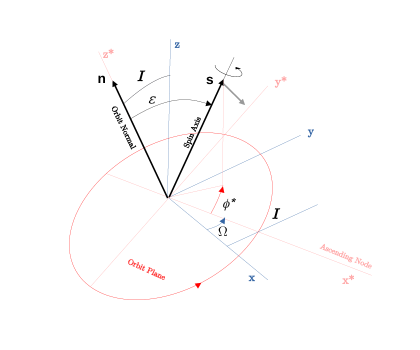
Figure 1: Inertial (fixed) coordinate system ($x,y,z$, blue) and coordinate system moving with the orbit plane ($x^{*},y^{*},z^{*}$, red), with $z^{*}$ parallel to the orbit normal $n$ and $x^{*}$ along the ascending node. $s$ is the spin axis, the obliquity (axial tilt) $\epsilon$ is the angle between $s$ and $n$ ($\cos\mbox{$\epsilon$}=\mbox{$\mbox{\boldmath$n$}$}\cdot\mbox{$\mbox{\boldmath$s$}$}$). $\Omega$ is the longitude of the ascending node, $I$ is the orbital inclination (angle between $z^{*}$ and $z$), and $\mbox{$\phi$}^{*}$ measures the precession angle in the orbit plane (see text).

For Earth, we write $\alpha$ as (e.g., Quinn et al., 1991):

$$\mbox{$\alpha$}=K\ (\mbox{$\kappa$}+\mbox{$\beta$})\ ,$$ (3)

where $\mbox{$\kappa$}=(1-e^{2})^{-3/2}$ and $e$ is the orbital eccentricity. $K$ and $\beta$ relate to the torque due to the Sun and Moon, respectively:

$$K = \frac{3}{2}\frac{C-A}{C}\frac{1}{\mbox{$\omega$}a^{3}}GM$$ (4)

$$\beta = g_{L}\ \frac{a^{3}}{R^{3}}\frac{m_{L}}{M}\ ,$$ (5)

where $A$ and $C$ are the planet’s equatorial and polar moments of inertia, $(C-A)/C=\mbox{$E_{d}$}$ is the dynamical ellipticity, $\omega$ is the planet’s angular speed, $a$ the semi-major axis of its orbit, $R$ is the Earth-Moon distance parameter, and $GM$ is the gravitational parameter of the Sun (see Table 1). The index ’$L$’ refers to lunar properties, where $g_{L}$ is a correction factor related to the lunar orbit (Kinoshita, 1975, 1977; Quinn et al., 1991) and $m_{L}/M$ is the lunar to solar mass ratio. The parameter values used for Earth are given in Table 1. The luni-solar precession $\Psi$ at $t_{0}$ is given by:

$$\mbox{$\Psi_{0}$}=-\dot{\phi}_{0}=-d\mbox{$\phi$}_{0}/dt=K(\mbox{$\kappa$}+\mbox{$\beta$})\cos\mbox{$\epsilon$}_{0}+\mbox{$\gamma_{gp}$}\ ,$$ (6)

where $\mbox{$\phi$}_{0}$ and $\mbox{$\epsilon$}_{0}$ are the precession and obliquity angle at $t_{0}$ ($d\mbox{$\phi$}_{0}/dt<0$, retrograde precession along the ecliptic), and $\gamma_{gp}$ is the geodetic precession (see Table 1). The geodetic precession was included in our numerical routines for Earth as described in Appendix A. Earth’s dynamical ellipticity $E_{d}$ at $t=t_{0}$ was determined from Eqs. (4) and (6) by setting the value for $\Psi_{0}$ (Capitaine et al., 2003, see Table 1). The value of $E_{d}$ in a particular precession model depends on the choice of $\Psi_{0}$ (see, e.g., Quinn et al., 1991; Laskar et al., 1993; Chen et al., 2015).

Table 1: Notation and values used in this paper.

Symbol	Meaning	Value I/A	Unit	Note
$\epsilon$	Obliquity angle		deg
$\epsilon$0	Obliquity Earth $t_{0}$	23.4392911	deg	Fränz & Harper (2002)
$\epsilon$0M	Obliquity Mars $t_{0}$	25.189417	deg	Folkner et al. (1997)
$\phi$	Precession angle
$s$	Spin vector
$n$	Orbit normal
$e$	Orbital eccentricity
$\varpi$	Orbit LP  a
$I$	Orbital inclination
$\Omega$	Orbit LAN  b
$\gamma_{gp}$	Geodetic precession	$-0.0192$	′′/y	Capitaine et al. (2003)
au	Astronomical unit	$1.495978707\mbox{$\times 10^{11}$}$	m
$GM$	Sun GP c	$1.32712440041\mbox{$\times 10^{20}$}$	$\rm m^{3}~{}s^{-2}$
$M/(m_{E}+m_{L})$	Mass ratio d	$328900.5596$	–
$m_{E}/m_{L}$	Mass ratio	$81.300568$	–
$\omega$	Earth’s angular speed	$7.292115\mbox{$\times 10^{-5}$}$	s-1	at $t_{0}$
$R_{0}$	Earth-Moon DP e	$3.8440\mbox{$\times 10^{8}$}$	m	at $t_{0}$, Quinn et al. (1991)
$A,C$	Moments of inertia f
$E_{d0}=(C-A)/C$	Earth’s dyn. ellipticity	$0.00327381$	–	at $t_{0}$, see text
$g_{L}$	Lunar orbit factor	$0.9925194$		see text
$\Psi_{0}$	$\dot{\phi}_{0}$ Earth	$50.384815$	′′/y	Capitaine et al. (2003)
$\Psi_{\rm 0M}$	$\dot{\phi}_{0}$ Mars	$7.597$	′′/y	Yoder et al. (2003)

2.1.2 Mars: Precession constant

For Mars $\mbox{$\beta$}=0$, while $K$ was determined from the observed $\Psi_{\rm 0M}$ and $\mbox{$\epsilon$}_{\rm 0M}$ (Folkner et al., 1997; Yoder et al., 2003, see Table 1):

$$K=\mbox{$\Psi_{\rm 0M}$}/(\cos\mbox{$\epsilon$}_{\rm 0M}\cdot\mbox{$\kappa$}_{\rm 0M})\ ,$$ (7)

where $\mbox{$\kappa$}_{\rm 0M}=(1-e_{\rm{}_{0M}}^{2})^{-3/2}$ and $e_{\rm{}_{0M}}$ is Mars’ orbital eccentricity at $t_{0}$. To first order, there is no averaged torque on Mars from its moons Phobos and Deimos (Laskar et al., 2004). Our numerical integrations (see Section 3.3) confirmed that Mars’ obliquity is chaotic (e.g., Touma & Wisdom, 1993; Laskar et al., 2004), i.e., is unpredictable on time scales beyond $\mbox{$\sim$}10^{7}$ y (although, see Bills & Keane, 2019). As the present study focuses on time scales $>$$10^{7}$ y, no attempt was made to include second-order effects on Mars’ computed precession and obliquity such as relativistic corrections, etc.

2.1.3 Coordinate systems and initial conditions

Orbital motion, spin axis motion, precession, etc. may be described in different coordinate systems. For example, the orbital motion may be described in an inertial frame defined by Earth’s mean orbit at J2000 (hereafter ECLIPJ2000), or in the Heliocentric Inertial (HCI) frame, etc. (see e.g., Fränz & Harper, 2002, naif.jpl.nasa.gov). The initial spin axis position, the precession angle, etc. may be conveniently described in a non-inertial frame defined by the instantaneous orbit plane (IOP) with the $z$-axis parallel to the orbit normal and the $x$-axis along the line of the ascending node (see Fig. 1). Our integrations for the orbital motion of the solar system were performed in a coordinate system equivalent to the HCI frame to conveniently account for the solar quadrupole moment (see Section 2.3 and Zeebe (2017)). The transformation between the different frames is accomplished by some form of Euler transformation (rotation matrix). For example, let $s$ and $\mbox{$\mbox{\boldmath$s$}$}^{*}$ be the spin vector in the inertial and IOP frame, respectively. Then (e.g., Ward, 1974):

$$\mbox{$\mbox{\boldmath$s$}$}^{*}={\cal{A}}_{(I,\Omega)}\ \mbox{$\mbox{\boldmath$s$}$}\ ,$$ (8)

where $I$ and $\Omega$ are the orbital inclination and longitude of ascending node, respectively, and ${\cal{A}}_{(I,\Omega)}$ is the time-dependent Euler transformation:

$${\cal{A}}_{(I,\Omega)}=\left(\begin{array}[]{ccc}\cos\mbox{$\Omega$}&\sin\mbox{$\Omega$}&0\\ -\cos I\sin\mbox{$\Omega$}&\cos I\cos\mbox{$\Omega$}&\sin I\\ \sin I\sin\mbox{$\Omega$}&-\sin I\cos\mbox{$\Omega$}&\cos I\end{array}\right)\ .$$ (12)

The static transformation matrix from ECLIPJ2000 to our HCI frame is given by ${\cal{A}}_{(I_{\sun},\Omega_{\sun})}$, where $I_{\sun}=7.155\arcdeg$ and $\Omega_{\sun}=75.594\arcdeg$ (see Zeebe, 2017). The static transformation matrix from Earth’s mean equator frame at J2000 to ECLIPJ2000 is given by ${\cal{A}}_{(\mbox{$\epsilon$}_{0},0)}$, where $\mbox{$\epsilon$}_{0}=23.4392911\arcdeg$.

The initial position of the spin vector in Earth’s mean equator frame at $t=0$ (J2000) was set to $\mbox{$\mbox{\boldmath$s$}$}^{\prime}_{0}=[0,0,1]$. The numerical spin axis integration (see Section 2.1.4) is carried out in our inertial HCI frame, in which $\mbox{$\mbox{\boldmath$s$}$}_{0}$ is given by $\mbox{$\mbox{\boldmath$s$}$}_{0}={\cal{A}}_{(I_{\sun},\Omega_{\sun})}{\cal{A}}_{(\mbox{$\epsilon$}_{0},0)}\mbox{$\mbox{\boldmath$s$}$}_{0}^{\prime}$.

The inclination of Earth’s and Mars’ orbit is referenced below in the invariable frame, i.e., relative to the invariable plane (perpendicular to the total angular momentum vector), a natural, common reference frame for solar system bodies. For example, the transformation of a state vector $X$ from ECLIPJ2000 to the invariable plane is given by $\mbox{\boldmath$X$}_{ip}={\cal{A}}_{(I_{ip},\Omega_{ip})}\mbox{\boldmath$X$}$, where $I_{ip}=1.5787\arcdeg$ and $\Omega_{ip}=107.5823\arcdeg$ (Souami & Souchay, 2012). The usual conversion is applied to switch between state vectors and orbital (Keplerian) elements.

2.1.4 Spin vector integration

The numerical integration of the spin vector $\mbox{$\mbox{\boldmath$s$}$}=[s_{x},s_{y},s_{z}]$ employed here follows Ward (1979); Bills (1990). Rewriting the orbit normal vector $n$ in terms of $p$ and $q$ as defined in Eq. (19) and substituting into Eq. (1) leads to:

$$\dot{s_{x}} = A\ (c_{1}s_{y}+c_{2}\mbox{$\tilde{q}$}s_{z})$$

$$\dot{s_{y}} = A\ (-c_{1}s_{x}+c_{2}\mbox{$\tilde{p}$}s_{z})$$ (13)

$$\dot{s_{z}} = A\ (-c_{2}(\mbox{$\tilde{q}$}s_{x}+\mbox{$\tilde{p}$}s_{y}))\ ,$$

where $A=\mbox{$\alpha$}[c_{2}(\mbox{$\tilde{p}$}s_{x}-\mbox{$\tilde{q}$}s_{y})+c_{1}s_{z}]/(1-e^{2})^{3/2}$, $c_{1}=\cos(I)$, $c_{2}=\cos(I/2)$. $\mbox{$\tilde{q}$}=2q$ and $\mbox{$\tilde{p}$}=2p$, where $p$ and $q$ are supplied by our astronomical solution ZB18a (see Section 2.3). The numerical spin vector integration is straightforward, fast, and provides a simple check on accuracy. As $s$ is a unit vector, $\delta=|\mbox{$\mbox{\boldmath$s$}$}|-1$ may be used to track the numerical error during the integration. A 100 Myr integration typically takes $\sim$3 sec (Linux, Intel i7-10875H, 2.30GHz) with $|\delta|<1\mbox{$\times 10^{-7}$}$. Our numerical routine in C is available at www2.hawaii.edu/~zeebe/Astro.html.

The obliquity $\epsilon$ may be calculated from Eq. (2) at any given time step, once the solution for $s$ has been obtained. The precession angle $\mbox{$\phi$}^{*}$ is measured in the IOP frame ($\mbox{$\phi$}^{*}=\mbox{atan}(s^{*}_{y},s^{*}_{x})$) with $\mbox{$\phi$}^{*}_{0}=90\arcdeg$ at $t=0$, hence we apply the transformation:

$$\mbox{$\mbox{\boldmath$s$}$}^{*}={\cal{A}}^{-1}_{(0,\Omega_{\sun})}\ {\cal{A}}_{(I,\Omega)}\ \mbox{$\mbox{\boldmath$s$}$}\ ,$$ (14)

which gives $\mbox{$\phi$}^{*}$ relative to the moving equinox. To obtain $\phi$ relative to the fixed equinox at J2000, we further apply ${\cal{A}}^{-1}_{(0,\Omega-\pi/2)}\mbox{$\mbox{\boldmath$s$}$}^{*}$, where the $\pi/2$-rotation accounts for the angle between the $x^{*}$-axis and $\mbox{$\mbox{\boldmath$s$}$}^{*}$’s component in the $x^{*}y^{*}$-plane at $t=0$, which points along the $y^{*}$-axis ($s^{*}_{x}=0$, see Fig. 1).

2.2 Earth: Tidal dissipation and dynamical ellipticity

Tidal dissipation, $T_{d}$, refers to the energy dissipation in the earth and ocean, which reduces Earth’s rotation rate and increases the length of day (LOD) and the Earth-Moon distance. The parameter relevant here for the precession-obliquity solution is the change in lunar mean motion $n$, which is presently ($t=t_{0}$) decreasing at a rate:

$$\mbox{$T_{d}$}_{0}=(\dot{n}/n)_{0}=-4.6\mbox{$\times 10^{-18}$}\ \mbox{s\mbox{${}^{-1}$}}$$ (15)

(Quinn et al., 1991). Given $n\propto R^{-3/2}$, where $R$ is the Earth-Moon distance parameter (see Table 1), it follows $\dot{R}/R=-\frac{2}{3}\ (\dot{n}/n)$. Dynamical ellipticity, $E_{d}$, refers to Earth’s gravitational shape, largely controlled by the hydrostatic response to its rotation rate. $E_{d}$ is proportional to $\omega^{2}$, where $\omega$ is Earth’s spin (see Table 1). Hence from Eq. (4) follows $\dot{K}/K=\dot{\omega}/\omega$ and from Eq. (5) $\dot{\beta}/\beta=-3\dot{R}/R=2(\dot{n}/n)$. Note that the input arguments for our C routine are non-dimensional, effective parameters, relative to the modern values, i.e., $\vartheta=\mbox{$T_{d}$}/\mbox{$T_{d}$}_{0}$ and $\eta=\mbox{$E_{d}$}/E_{d0}$.

Changes in $T_{d}$ and $E_{d}$ over time cause slow changes in $K$ and $\beta$ (see Eqs. (4) and (5)). Following Quinn et al. (1991), these may be approximated to vary linearly with time (insert $\dot{K}/K$ and $\dot{\beta}/\beta$ from above):

$$K = K_{0}\ [1+(\dot{\omega}/\omega)_{0}\ (t-t_{0})]$$ (16)

$$\beta = \beta_{0}\ [1+2(\dot{n}/n)_{0}\ (t-t_{0})]\ ,$$ (17)

where $(\dot{n}/n)_{0}$ is given by Eq. (15) and $(\dot{\omega})_{0}\simeq 51(\dot{n})_{0}$ (Lambeck, 1980). While $T_{d}$ and $E_{d}$ have significant effects on Earth’s precession and obliquity frequencies (Zeebe & Lourens, 2022a), their effect on, for instance, Earth’s obliquity amplitude (which is relevant here) is small. In this study, the default values $\vartheta=1$ and $\eta=1$ were used and the precession constant $\alpha$ as a function of time calculated using Eqs. (3), (16), and (17). The parameters $\vartheta$ and $\eta$ may be varied for other purposes such as geologic dating (Zeebe & Lourens, 2022a). By default, additional long-term effects of tidal dissipation on obliquity (secular trend) were not included here. However, our C code provides this option, available at www2.hawaii.edu/~zeebe/Astro.html.

2.3 Solar system integration

For the present study, we use our astronomical solution ZB18a (see below), described in detail in Zeebe & Lourens (2019). Hence we only provide a brief summary of the integrations methods here. Solar system integrations were performed following our earlier work (Zeebe, 2015a, b, 2017; Zeebe & Lourens, 2019, 2022b) with the integrator package HNBody (Rauch & Hamilton, 2002) (v1.0.10) using the symplectic integrator and Jacobi coordinates (Zeebe, 2015a). All simulations include contributions from general relativity (Einstein, 1916), available in HNBody as Post-Newtonian effects due to the dominant mass. The Earth-Moon system was modeled as a gravitational quadrupole (Quinn et al., 1991) (lunar option), shown to be consistent with expensive Bulirsch-Stoer integrations up to 63 Ma (Zeebe, 2017). Initial conditions for the positions and velocities of the planets and Pluto were generated from the JPL DE431 ephemeris (Folkner et al., 2014) (naif.jpl.nasa.gov/pub/naif/generic_kernels/spk/planets), using the SPICE toolkit for Matlab (naif.jpl.nasa.gov/naif/toolkit.html). We have recently also tested the latest JPL ephemeris DE441 (Park et al., 2021), which has no effect on the current results because the divergence time relative to ZB18a (based on DE431) is $\sim$66 Ma. The integrations for ZB18a (Zeebe & Lourens, 2019) included 10 asteroids, with initial conditions generated at ssd.jpl.nasa.gov/x/spk.html (for a list of asteroids, see Zeebe (2017)). Coordinates were obtained at JD2451545.0 in the ECLIPJ2000 reference frame and subsequently rotated to account for the solar quadrupole moment ($J_{2}$) alignment with the solar rotation axis (Zeebe, 2017). Earth’s orbital eccentricity for the ZB18a solution is available at www2.hawaii.edu/~zeebe/Astro.html and www.ncdc.noaa.gov/paleo/study/35174. We provide our solutions over the time interval from 100-0 Ma. However, as only the interval 58-0 Ma is constrained by geologic data (Zeebe & Lourens, 2019), we solely focus on this particular interval here and caution that the interval prior to 58 Ma is unconstrained due to solar system chaos.

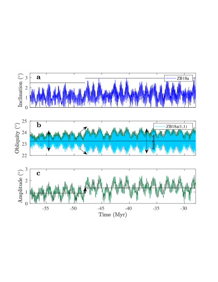
Figure 2: (a) Earth’s orbital inclination in the invariable frame from ZB18a. Horizontal lines indicate maximum values from 58-48 Ma and 48-0 Ma. (b) Earth’s obliquity, $\epsilon$, calculated using our spin vector integration. ZB18a(1,1) (light blue) is the default solution with tidal dissipation and dynamical ellipticity parameters $(\vartheta=1,\eta=1)$. The change in the obliquity variation around 48 Ma (arrows) may be illustrated using the envelope (Hilbert transform, $\mbox{${\cal H}$}(\mbox{$\epsilon$})$, green). (c) $2\mbox{${\cal H}$}(\mbox{$\epsilon$}-\overline{\mbox{$\epsilon$}})$ indicates a $\sim$50% increase at $\sim$48 Ma in the average amplitude around the mean obliquity value ($\overline{\mbox{$\epsilon$}}$).

3 Results

In the following, we report the results of our numerical solar system- and spin vector integrations. We focus on Earth and Mars, for which changes in orbital inclination around 48 Ma (see below) appear most pronounced and relevant to possible effects on planetary climate evolution. The results for Mercury’s orbit suggest only moderate changes in inclination pattern (not shown), while the results for Venus’ orbital inclination are similar to those for Earth.

3.1 Earth’s orbital inclination and obliquity

Numerical integration of the spin vector using our orbital solution ZB18a provides up-to-date solutions for Earth’s precession and obliquity as a function of tidal dissipation and dynamical ellipticity for geologic analyses (Zeebe & Lourens, 2022a). In terms of solar system dynamics, the results are consistent with expectations over the past $\sim$48 Ma (cf., e.g., Quinn et al., 1991; Laskar et al., 1993; Zeebe & Lourens, 2022a). However, from $\sim$58 to $\sim$48 Ma the obliquity shows significantly reduced variations (Fig. 2). The reduced obliquity variations are a direct result of the damped inclination amplitude in ZB18a across the same time interval (Fig. 2a). None of the spin vector integrations using any of the orbital solutions ZB17a-f (Zeebe, 2017), for instance, shows a similar behavior. The reason for the damped inclination amplitude prior to $\sim$48 Ma is a resonance transition (see Section 4) that occurs between $\sim$53 and $\sim$45 Ma in ZB18a (Zeebe & Lourens, 2022b), but at different times in other solutions such as ZB17a-f. The magnitude of the change in the obliquity variation around 48 Ma may be illustrated by calculating the obliquity envelope (Hilbert transform), indicating a $\sim$50% increase in the average amplitude around the mean obliquity value (Fig. 2c). Note that for Earth’s climate even small changes in obliquity are relevant (see discussion, Section 5).

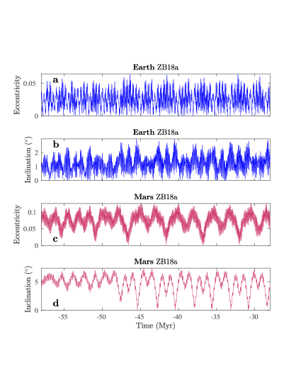
Figure 3: Earth’s and Mars’ orbital eccentricity and inclination in the invariable frame from ZB18a. Note the large change in the variation of Mars’ inclination around 48 Ma in (d).

3.2 Earth’s and Mars’ orbital eccentricity and inclination

While the change in Earth’s orbital eccentricity and inclination across $\sim$48 Ma may appear somewhat subtle, the change in Mars’ inclination variation is large (see Fig. 3). Mars’ inclination in the invariant frame varies between 3.1° and 7.1° from 58 to 48 Ma, but between almost 0° and 7.4° from 48 to 0 Ma, showing a distinct M-pattern (Fig. 3d). The M-pattern with near-zero values continues until the present. The M-pattern is also apparent in Mars’ eccentricity (Fig. 3c), albeit at twice the period than inclination from 48 to 0 Ma. Prior to 48 Ma, the period ratio is $\sim$1:1, with maxima in eccentricity roughly coinciding with minima in inclination, and illustrating the resonance transition in the solution ZB18a (see Section 4). Thus, our analysis suggests large changes in Mars’ orbital inclination and hence in the pattern of climate forcing on Mars around 48 Ma (see Section 3.3 and discussion, Section 5).

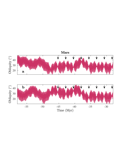
Figure 4: Mars’ obliquity calculated using our our spin vector integration with orbital solution ZB18a and two different values for the precession constant (see Eq. (7)). (a) $\mbox{$\Psi_{\rm 0M}$}=7.6083+0.0021$ ^′′/y and (b) $\mbox{$\Psi_{\rm 0M}$}=7.6083-0.0021$ ^′′/y (Konopliv et al., 2016). Arrows indicate nodes in obliquity (reduced variation) with a period of $\sim$2.4 Myr that are absent from $\sim$58-48 Ma.

3.3 Mars’ obliquity

As mentioned above, our integrations confirmed that Mars’ obliquity is chaotic (e.g., Touma & Wisdom, 1993; Laskar et al., 2004); that is, the details of Mars’ obliquity evolution are unpredictable on time scales beyond $\mbox{$\sim$}10^{7}$ y (although, see Bills & Keane, 2019). However, irrespective of the details, our orbital solution suggests a major shift in Mars’ inclination and hence in the pattern of Mars’ obliquity around 48 Ma. For example, we integrated sets of solutions with small differences in Mars’ precession constant (equal to reported error bounds), which all showed the same obliquity pattern (see Fig. 4). We tested several values for $\Psi_{\rm 0M}$ (see Table 1 and Eq. (7)), including $7.597\pm 0.025$ ^′′/y and $7.6083\pm 0.0021$ ^′′/y (Yoder et al., 2003; Konopliv et al., 2016). Even using the small uncertainty of 0.0021 ^′′/y, the obliquity solutions are different prior to $\sim$14 Ma due to chaos. However, the pattern before and after $\sim$48 Ma is the same (Fig. 4). Before $\sim$48 Ma, Mars’ obliquity varies continuously around a mean value at a given time with an approximate amplitude of $\sim$15-20°. After $\sim$48 Ma, Mars’ obliquity shows bundling into amplitude modulation (AM) “couples” with strong nodes (reduced variation) at a period of $\sim$2.4 Myr (arrows, Fig. 4) that are absent from $\sim$58-48 Ma. The timing of the nodes corresponds to the near-zero values in Mars’ inclination (see Figure 3). Around the nodes, Mars’ obliquity stays nearly constant for hundreds of thousands of years with variations $\lesssim 2\arcdeg$.

4 Solar system frequency analysis

To investigate the shift in Earth’s and Mars’ orbital inclination and changes in the fundamental proper modes, or eigenmodes, of the solar system around 48 Ma in ZB18a, we performed spectral analyses of the classic variables (e.g., Nobili et al., 1989; Laskar et al., 2011; Zeebe, 2017):

$$h=e\sin(\mbox{$\varpi$})\quad \quad k=e\cos(\mbox{$\varpi$})$$ ; (18)

$$p=\sin(I/2)\ \sin\mbox{$\Omega$}\quad \quad q=\sin(I/2)\ \cos\mbox{$\Omega$}\ ,$$ ; (19)

where $e$, $I$, $\varpi$, and $\Omega$ are eccentricity, inclination, longitude of perihelion, and longitude of ascending node, respectively. The quantities $(h,k)=\mbox{\boldmath$e$}$ and $(p,q)=\mbox{\boldmath$i$}$ may be referred to as eccentricity and inclination vector, respectively. For the frequency analyses, we use the variables $k$ and $q$ (equivalent to using $h$ and $p$) for Earth and Mars, and two time windows, one before and one after the transition around 48 Myr: Interval 1: [60 50] Ma and Interval 2: [46 36] Ma (see Figs. 5 and 6). Spectral analysis of $k$ and $q$ yield the fundamental frequencies of the solar system’s eigenmodes, $g$- and $s$-modes, respectively. The $g$-modes are loosely related to the perihelion precession of the planetary orbits, e.g., $g_{3}$ and $g_{4}$ to Earth’s and Mars’ orbits, etc. ($s$-modes correspondingly to the nodes). The $g$’s and $s$’s are constant in quasiperiodic systems but vary over time in chaotic systems. It is critical to recall that there is no simple one-to-one relation between planet and eigenmode, particularly for the inner planets. The system’s motion is a superposition of all eigenmodes, although some modes represent the single dominant term for some (mostly outer) planets. For the current problem, analysis of changes in the frequency bands around $g_{3}$ and $g_{4}$, and $s_{3}$ and $s_{4}$ are most instructive to examine, for instance, $(g_{4}-g_{3})$ and $(s_{4}-s_{3})$. Changes in other important frequencies such as $(g_{2}-g_{5})$ were found to be small on this time scale and across the transition around 48 Ma, consistent with earlier work (e.g., Laskar et al., 2011; Zeebe, 2017; Spalding et al., 2018).

The $g$- and $s$-modes are key to understanding secular resonances and the resonance transition. In simple orbital configurations, secular resonances refer to the commensurability of apsidal and nodal precessional frequencies, directly involving the orbital $\varpi$’s and $\Omega$’s (for review, see e.g., Murray & Dermott, 1999; Murray & Holman, 2001; Morbidelli, 2002). In the solar system, planetary secular resonances involve the $g$- and $s$-modes (see above) obtained through, e.g., $e$ and $i$ from numerical solutions. For example, in our orbital solution ZB18a, the ratio $(g_{4}-g_{3}):(s_{4}-s_{3})$ is $\sim$1:1 before $\sim$53 Ma (one resonance state) and $\sim$1:2 after $\sim$45 Ma (another resonance state, see Section 4.3 and Zeebe & Lourens, 2019, 2022b). Hence during the interval from $\sim$53 to $\sim$45 Ma the system switches from one secular resonance state to another, aka resonance transition. A resonance transition represents an unmistakable expression of chaos and does not exist in periodic and quasiperiodic systems. For instance, if the mutual planet-planet perturbations in the solar system were sufficiently small (all eccentricities and inclinations small), then the full dynamics could be described by linear secular perturbation theory (Laplace-Lagrange solution, e.g., Murray & Dermott, 1999; Morbidelli, 2002; Laskar et al., 2011; Zeebe, 2017). In the linear theory, the $g$- and $s$-modes are independent (do not interact) and resonance transitions are absent, which is hence insufficient to describe the chaotic nature of the solar system (see below and e.g., Batygin et al., 2015; Mogavero & Laskar, 2022).

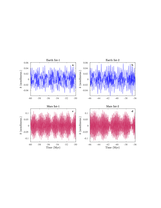
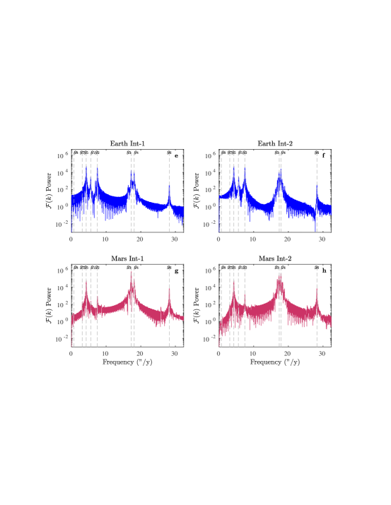
Figure 5: Time series analysis of $k=e\cos(\mbox{$\varpi$})$ for Earth and Mars (see text) to extract solar system $g$-modes from ZB18a. Int = Interval, ${\cal F}$ = Fast-Fourier Transform (FFT). Vertical dashed lines in (e-h) indicate frequencies of $g$-modes (see Zeebe, 2017).

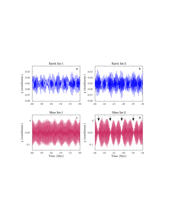
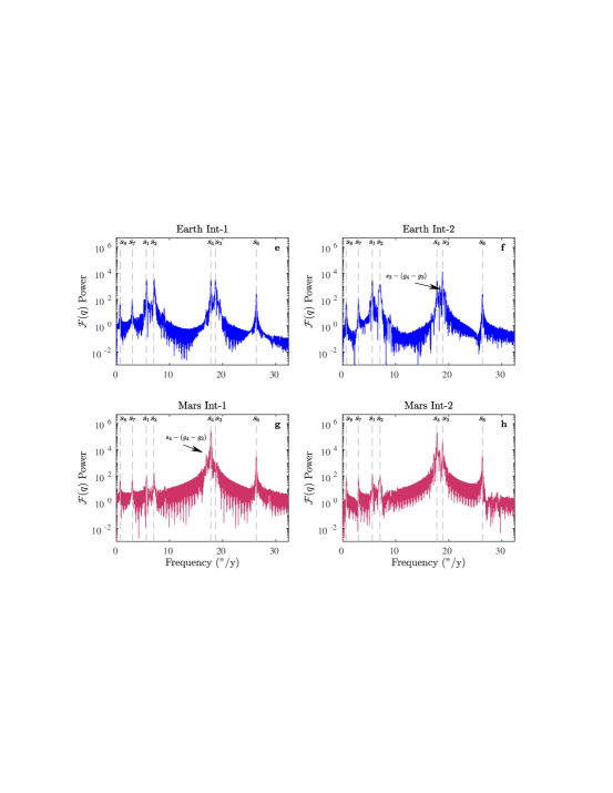
Figure 6: Time series analysis of $q=\sin(I/2)\cos\mbox{$\Omega$}$ for Earth and Mars (see text) to extract solar system $s$-modes from ZB18a. Int = Interval, ${\cal F}$ = Fast-Fourier Transform (FFT). Arrows in (d) indicate nodes (reduced amplitude, cf. Figure 4). Vertical dashed lines in (e-h) indicate frequencies of $s$-modes (see Zeebe, 2017).

4.1 Changes in $g$- and $s$-modes

Spectral analysis of $k$ from ZB18a shows that the relative power of $g_{3}$ and $g_{4}$ and their frequency difference $(g_{4}-g_{3})$ change significantly across the transition around 48 Ma (Fig. 5). Going forward in time, $g_{4}$’s relative power increases in both Earth’s and Mars’ $k$ spectra, while the frequency difference $(g_{4}-g_{3})$ drops by $\sim$36%. The changes are most apparent in Mars’ $k$ (Fig. 5d), showing an increase in the amplitude modulation (AM) period (also called beat period) from $P_{g}=(g_{4}-g_{3})\mbox{${}^{-1}$}\simeq 1.5$ Myr in Interval 1 to $\sim$2.4 Myr in Interval 2, i.e., a resonance transition (see Section 4.3). Conversely, $s_{3}$’s power increases relative to $s_{4}$ in both Earth’s and Mars’ $q$ spectra, while the frequency difference $(s_{4}-s_{3})$ rises by $\sim$24%. The changes are again most apparent in Mars’ $q$ (Fig. 6d), showing a decrease in the beat period from $\mbox{$\sim$}1.5$ Myr in Interval 1 to $\sim$1.1 Myr in Interval 2.

4.1.1 Earth

The maximum amplitude in both Earth’s $k$ and $q$ increases across the transition, although the increase is more pronounced in $q$ (Figs. 5 and 6, top panels). The change in Earth’s $q$ is related to the $s$-modes and hence to inclination and was analyzed in more detail (see also Section 4.2). Most obviously, $s_{3}$’s power in Earth’s $q$ spectrum almost quadruples (Fig. 6e and f), which should substantially increase $q$’s amplitude (everything else being equal). In addition, however, the power associated with $s_{2}$ and $s_{4}$ drops by about 70% and 25%, respectively (Fig. 6e and f) and a peak of discernible power appears in Earth’s $q$-spectrum between $s_{4}$ and $s_{3}$ in Interval 2 (Fig. 6f, arrow). The peak can be identified as $s_{3}-(g_{4}-g_{3})$, illustrating the interaction of $(g_{4}-g_{3})$ and $(s_{4}-s_{3})$; a feature almost certainly involved in the chaotic behavior of the system (e.g., Sussman & Wisdom, 1992; Laskar et al., 2011; Zeebe, 2017; Mogavero & Laskar, 2022). It turns out that the amplitude changes in $s_{1}$ through $s_{4}$ and the $s_{3}-(g_{4}-g_{3})$ peak are critical to reconstruct the overall rise in Earth’s $q$ amplitude (see Section 4.2). As a result, the shift in the variation in Earth’s orbital inclination and obliquity around 48 Ma is largely due to the contribution change in the superposition of the $s$-modes 1-4 and the $g$-$s$-mode interaction in the inner solar system. The $g$-$s$-mode interaction is also key to understanding the AM shift in Mars’ inclination vector (Section 4.1.2).

4.1.2 Mars

Across the transition, the AM in Mars’ $q$ intensifies, displaying bundling into AM “couples” with strong nodes (reduced amplitude) at twice the AM beat period (Fig. 6d, arrows). Remarkably, $s_{3}$ appears negligible for Mars’ $q$ in Interval 1. The spectral power at $s_{3}$’s frequency does not rise above the background level (Fig. 6g). Instead, some power is concentrated in one of $s_{4}$’s side peaks at lower frequency, identified as $s_{4}-(g_{4}-g_{3})$ (see Fig. 6g, arrow and Section 4.2). Interestingly, the combination of (difference between) $s_{4}$ and $s_{4}-(g_{4}-g_{3})$ effectively leads to the same AM period as $(s_{4}-s_{3})$ because $(s_{4}-s_{3})$ and $(g_{4}-g_{3})$ are indistinguishable in Interval 1 within errors (see Section 4.3). Thus, the $\sim$1.5 Myr beat in Mars’ $q$ in Interval 1 is actually due to $g$-modes, not $s$-modes, again illustrating the interaction of $(g_{4}-g_{3})$ and $(s_{4}-s_{3})$ and its likely involvement in the system’s resonances and chaos (Section 4.3).

The nodes in Mars’ $q$ at twice the AM beat period in Interval 2 (Fig. 6d, arrows) correspond to the minima near zero in inclination (cf. Fig. 3d) and to the nodes in Mars’ obliquity (cf. arrows in Fig. 4). As a result, the change in the variation of Mars’ orbital inclination and obliquity across the transition around 48 Ma can be traced back to the changes in amplitude and frequency of the $g$- and $s$-modes. That is, here largely to a stronger expression of $s_{3}$ in Mars’ orbit, causing a stronger AM in Mars’ inclination vector due to $(s_{4}-s_{3})$. The effect of changes in the $g$- and $s$-modes on Earth’s and Mars’ inclination vectors as inferred above are corroborated by a basic model of signal reconstruction using only key eigenmodes (Section 4.2).

4.2 Signal reconstruction using key eigenmodes

Table 2: Reconstruction of Earth’s $q$ (see Eq. (20)).

$f_{i}$	$f_{i}$ a	$T_{i}$	$A_{i}$	$\mbox{${\cal F}$}_{i}(q)$ b	$\mbox{$\varphi$}_{i}$
	(′′/y)	(kyr)	($\times 10^{3}$)	($\times 10^{-3}$)	(rad)
	60-50 Ma
$s_{2}$	$-7.08$	183.01	$-5.23$	$4.27$	$-0.083$
$s_{4}$	$-17.79$	72.84	$-4.89$	$3.73$	$-0.622$
$s_{3}$	$-18.64$	69.53	$-4.75$	$3.53$	$1.128$
$s_{1}$	$-5.67$	228.67	$-4.44$	$3.08$	$3.071$
	46-36 Ma
$s_{3}$	$-18.84$	68.79	$-8.99$	$12.63$	$1.224$
$s_{1}$	$-5.61$	231.00	$-4.24$	$2.81$	$-2.046$
$s_{4}$	$-17.79$	72.83	$-4.20$	$2.75$	$-1.326$
$s_{2}$	$-7.14$	181.61	$-3.00$	$1.41$	$0.392$
$s_{3}-(g_{4}-g_{3})$	$-18.31$	70.77	$-2.72$	$1.15$	$3.961$

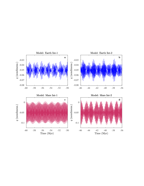
Figure 7: Reconstruction of Earth’s and Mars’ $q$ using only key eigenmodes (see Eq. (20)). The reconstructed time series correspond to Figures 6a-d from the full solar system integration (solution ZB18a).

Table 3: Reconstruction of Mars’ $q$ (see Eq. (20)).

$f_{i}$	$f_{i}$ a	$T_{i}$	$A_{i}$	$\mbox{${\cal F}$}_{i}(q)$ b	$\mbox{$\varphi$}_{i}$
	(′′/y)	(kyr)	($\times 10^{3}$)	($\times 10^{-3}$)	(rad)
	60-50 Ma
$s_{4}$	$-17.79$	72.85	$-45.25$	$319.90$	$0.162$
$s_{4}-(g_{4}-g_{3})$	$-16.94$	76.49	$-5.12$	$4.10$	$0.999$
$s_{6}$	$-26.35$	49.18	$-4.53$	$3.21$	$3.307$
	46-36 Ma
$s_{4}$	$-17.78$	72.89	$-36.04$	$202.94$	$1.576$
$s_{3}$	$-18.85$	68.76	$-17.32$	$46.87$	$2.832$
$s_{4}-(g_{4}-g_{3})$	$-17.23$	75.24	$-5.61$	$4.91$	$0.153$
$s_{6}$	$-26.34$	49.20	$-4.62$	$3.33$	$-1.048$

To quantitatively assess the effect of changes in the $g$- and $s$-modes on Earth’s and Mars’ inclination vectors as described above, we use a basic model of signal reconstruction, selecting only a few key eigenmodes. For example, Earth’s and Mars’ $q$ were reconstructed using:

$$q=\sum A_{i}\cos(2\pi f_{i}t+\mbox{$\varphi$}_{i})+C\ ,$$ (20)

where $A_{i}$, $f_{i}$, and $\mbox{$\varphi$}_{i}$, are the amplitude, frequency, and phase of the selected eigenmode $i$. $A$’s and $f$’s were directly taken from the FFT analysis, while $\mbox{$\varphi$}_{i}$’s were fit using non-linear least squares to allow for adjustment of possible mismatches due to the omission of non-critical modes. Note that the power $\mbox{${\cal F}$}(q)$ in the FFT spectrum is proportional to the square of the wave amplitude $A$, e.g., for a single cosine wave, $\mbox{${\cal F}$}(q)\propto A^{2}/4$. Modes included in the reconstruction that significantly reduce the root-mean square deviation (RMSD) between Eq. (20) and $q$ from our astronomical solution ZB18a are considered essential. In addition, the mode selection was tested using the Lasso method (Least absolute shrinkage and selection operator, Tibshirani, 1996), as applied to frequency analysis (e.g., Kato & Uemura, 2012). The Lasso technique tends to produce some coefficients (such as the $A_{i}$’s in Eq. (20)) that are exactly zero and hence should yield more easily interpretable models. Application to the current problem following Kato & Uemura (2012) largely confirmed the mode selection based on RMSD, although the Lasso method appeared sensitive to the chosen frequency window and resolution (resulting in variable relative power of different modes).

For Earth’s $q$, a set of four and five modes, respectively, turned out to be essential for the signal reconstruction in Interval 1 and 2 (see Table 2 and Fig. 7). As discussed in Section 4.1.1, the five modes in Interval 2 include $s_{3}-(g_{4}-g_{3})$, i.e., the peak between $s_{4}$ and $s_{3}$, highlighting the $g$-$s$-mode interaction. For Mars’ $q$, a set of three and four modes, respectively, turned out to be essential in Interval 1 and 2 (see Table 3 and Fig. 7). The presence of $s_{4}-(g_{4}-g_{3})$ is essential for the AM in Interval 1, while the rise in $s_{3}$’s power across the transition is the most important change to explain the substantial increase in AM and the strong nodes in Mars’ $q$ in Interval 2. In summary, the characteristic features of Earth’s and Mars’ inclination vectors before and after the transition around 48 Ma can be reconstructed using a few key eigenmodes (compare Figs. 6 and 7). The reconstruction confirms that the shifts in the variation in Earth’s and Mars’ orbital inclination and obliquity around 48 Ma are due to contribution changes in the superposition of $s$-modes, plus the $g$-$s$-mode interaction in the inner solar system.

4.3 $(g_{4}-g_{3}):(s_{4}-s_{3})$ Resonance

The results of the spectral analysis for $k$ and $q$ (Figs. 5 and 6) suggest ratios for $(g_{4}-g_{3}):(s_{4}-s_{3})$ very close to 1:1 and 1:2 in Interval 1 and and 2, respectively. However, examining whether or not these ratios represent exact resonances requires evaluation of the uncertainties in the frequency differences and hence uncertainties in the individual $g$’s and $s$’s. Based on literature estimates and several tests performed here (see Appendix B), we take $\mbox{$\Delta$}f\simeq 6.5\mbox{$\times 10^{-3}$}$ ^′′/y $=5\mbox{$\times 10^{-6}$}$ kyr^-1 as an estimated uncertainty in determining the individual frequencies $g_{3},g_{4},s_{3}$, and $s_{4}$ from our solar system integrations. Note that the present uncertainty estimates do generally not apply to noisy geologic data. In the following, we focus on the periods of the amplitude modulation (or beats, e.g., $P_{g}=(g_{4}-g_{3})\mbox{${}^{-1}$}$), rather than frequencies, as the beats can be identified in the geologic record ($P_{g}\simeq P_{s}\simeq 1.5$ Myr in Interval 1 and $P_{g}\simeq 2.4$ Myr, $P_{s}\simeq 1.2$ Myr in Interval 2). Error propagation then yields for the uncertainties ($\mbox{$\Delta$}P$) in the beat periods:

$$\mbox{$\Delta$}P_{g}=\sqrt{2}\ \frac{\mbox{$\Delta$}f}{(g_{4}-g_{3})^{2}}\quad;\quad\mbox{$\Delta$}P_{s}=\sqrt{2}\ \frac{\mbox{$\Delta$}f}{(s_{4}-s_{3})^{2}}\ .$$ (21)

The largest uncertainties are expected in Interval 2 with the smallest $(g_{4}-g_{3})$, which gives $\mbox{$\Delta$}P_{g}\simeq 40$ kyr and $\mbox{$\Delta$}P_{s}\simeq 10$ kyr. Given the period ratio of $\sim$2:1 in Interval 2, the uncertainty bound for $P_{g}-2P_{s}$ is hence $\simeq 40+2\times 10\simeq 60$ kyr. Spectral analysis using FFT and the multi-taper method (MTM) in Interval 1 (Earth’s $k$ and $q$) yielded $P_{g}-P_{s}\simeq 0$ and 5 kyr, respectively. In Interval 2 (Earth’s $k$ and $q$), FFT and MTM yielded $P_{g}-2P_{s}\simeq 80$ and 6 kyr, respectively (30 and 6 kyr using Mars’ $k$ and $q$).

Within errors, the results of the spectral analysis for $k$ and $q$ (Figs. 5 and 6) therefore indeed suggest a 1:1 and 2:1 resonance in Interval 1 and 2, respectively. The slightly larger $P_{g}-2P_{s}$ from FFT in Interval 2 (80 kyr, Earth’s $k$ and $q$) is unlikely to be significant. First, the result is not confirmed using FFT and Mars’ $k$ and $q$, or MTM. Second, extending Interval 2 by, say, 0.5 Myr toward the present, yields $P_{g}-2P_{s}\simeq 6$ kyr, indicating additional sensitivity to window selection and length. Third, the uncertainty in the individual frequencies ($\mbox{$\Delta$}f$) could be somewhat larger than the $5\mbox{$\times 10^{-6}$}$ kyr^-1 assumed here (see Appendix B).

5 Summary and Discussion

Analysis of our optimal orbital solution ZB18a shows that solar system chaos caused reduced variations in Earth’s and Mars’ orbital inclination and Earth’s obliquity from $\sim$58 to $\sim$48 Ma. We applied time series analyses and signal reconstruction using key eigenmodes to extract and investigate changes in solar system frequencies. Both approaches highlight changes in the superposition of $s$-modes and the involvement and interaction of $(g_{4}-g_{3})$ and $(s_{4}-s_{3})$ in explaining changes in inclination and obliquity around 48 Ma. The $g$-$s$-mode interactions in the inner solar system (e.g., Sussman & Wisdom, 1992; Laskar et al., 2011; Zeebe, 2017; Mogavero & Laskar, 2022) and the resonance transition (Zeebe & Lourens, 2019) represent unmistakable expressions of chaos in the solar system. Dynamical chaos hence not only affects the solar system’s orbital properties, but also the long-term evolution of planetary climate through eccentricity and the link between inclination and axial tilt.

For Earth’s climate even small changes in obliquity are relevant because obliquity controls the seasonal contrast through changes in insolation — particularly important in high latitudes. For instance, over the past few million years, obliquity was a major forcing factor and pacemaker for the ice ages (e.g., Hays et al., 1976; Paillard, 2021). Hence reduced variations in Earth’s obliquity from $\sim$58 to $\sim$48 Ma should also have affected Earth’s climate across this time interval (aka the late Paleocene — early Eocene, LPEE). Remarkably, a nearly ubiquitous phenomenon in long-term geologic records across the LPEE is a very weak or absent obliquity signal (e.g., Lourens et al., 2005; Westerhold et al., 2007; Littler et al., 2014; Zeebe et al., 2017; Barnet et al., 2019). We do not rule out that other factors such as the greenhouse climate at the time, the absence of large ice sheets, etc. may have contributed to a weak expression of obliquity (high-latitude) forcing as well. However, strong obliquity signals have been identified during other greenhouse episodes such as the mid-Cretaceous climate optimum in mid-latitude/equatorial sites (e.g., Meyers, 2012), indicating that more than just high temperatures were necessary to suppress the obliquity signal in LPEE records. Notably, based on the expression of orbital cycles in the sedimentary record, Vahlenkamp et al. (2020) tuned their astronomical age model solely to eccentricity cycles during the early Eocene ($\sim$56 to $\sim$47 Ma) but to a mix of eccentricity and obliquity cycles during the middle Eocene ($\sim$48 to $\sim$40 Ma), indicating the onset of a stronger obliquity component around 48 Ma. We propose here that the reduced amplitude in Earth’s obliquity, as predicted by our astronomical solution ZB18a, contributed to the weak/absent obliquity signal in geologic records from $\sim$58 to $\sim$48 Ma.

As for Earth, astronomical theories of climate (Milanković, 1941) also have a long history for Mars (e.g., Pollack, 1979; Toon et al., 1980). Of particular interest here is the primary control of obliquity on the exchange of CO₂ and H₂O between Mars’ surface reservoirs and polar caps on time scales of $10^{5}-10^{6}$ years (e.g., Armstrong et al., 2004; Levrard et al., 2007; Vos et al., 2019; Buhler & Piqueux, 2021). Modeling suggests that CO₂ fluxes may be assumed in equilibrium on obliquity time scales (Buhler & Piqueux, 2021). Hence the instantaneous, absolute value of obliquity would be the critical control variable for, e.g., the mass of CO₂ stored in Mars’ atmosphere, polar cap, and regolith; memory effects would be small. On the contrary, memory effects are significant for, e.g., water ice stored in tropical/mid-latitude surface reservoirs and Mars’ polar layered deposits. For example, estimates for the buildup time of the north-polar layered deposits to its current size are of the order of 4 Myr, with accelerated growth during intervals of small and relatively constant obliquity (Levrard et al., 2007; Vos et al., 2019). Hence for the mass of H₂O stored in Mars’ surface reservoirs, both the absolute value of obliquity, as well as its temporal evolution (pattern) are the critical control variables.

Our optimal astronomical solution suggests significant changes in Mars’ orbital inclination and obliquity pattern around 48 Ma (see Figs. 3 and 4). For example, intervals of relatively constant obliquity (or nodes, see arrows, Fig. 4) are absent from $\sim$58 to $\sim$48 Ma. Thus, rapid growth periods of polar layered deposits at low obliquity would not exist during this time period, which should be recorded in Mars’ climate archives (although not in the current north-polar layered deposits if the maximum age is $\sim$4 Ma). Note that while the detailed long-term evolution of Mars’ obliquity is unknown prior to $\sim$10-15 Ma, low-obliquity states are likely throughout its history (e.g., Laskar et al., 2004; Armstrong et al., 2004; Fassett et al., 2014; Holo et al., 2018; Bills & Keane, 2019; Jakosky, 2021). If suitable long-term climate/obliquity records exist on Mars, they should also show the onset of bundling into amplitude modulation “couples” with strong nodes (reduced obliquity variation) around 48 Ma with a period of $\sim$2.4 Myr; and their absence from $\sim$58 to $\sim$48 Ma (Fig. 4). Interestingly, Smith et al. (2020) recently laid out a road map for unlocking the climate record stored in Mars’ north-polar layered deposits, including a final mission to analyze $\sim$500 m of vertical section. The section would allow accessing $\sim$1 Myr of martian climate history (if feasible, probably at most $\sim$4 Myr for longer sections). Thus, unlocking Mars’ climate history on 10-100 Myr time scales to reveal the workings of chaos in the solar system would require different strategies.

Appendix A Geodetic precession

For Earth, we also include the relatively small contribution from geodetic precession (GP) to the total precession $\phi$, say, $\dot{\phi}_{gp}=\mbox{$\gamma_{gp}$}$, which represents a differential equation in terms of $\phi$. However, we integrate here a differential equation for $s$ (see Eq. (1)). GP acts along the direction of $(\mbox{$\mbox{\boldmath$s$}$}\times\mbox{$\mbox{\boldmath$n$}$})$, hence we use an ansatz in the form of Eq. (1) to include GP:

$$\dot{\mbox{$\mbox{\boldmath$s$}$}}=\mbox{$\tilde{\gamma}_{gp}$}\cdot\mbox{$\alpha$}\ (\mbox{$\mbox{\boldmath$n$}$}\cdot\mbox{$\mbox{\boldmath$s$}$})(\mbox{$\mbox{\boldmath$s$}$}\times\mbox{$\mbox{\boldmath$n$}$})\ ,$$ (A1)

where the factor $\tilde{\gamma}_{gp}$ may be determined as follows. Let $s_{x}$ and $s_{y}$ be the $s$-components in the orbit plane at $t_{0}$ (cf. Fig. 1, omit asterisks). At $t_{0}$, $s_{x}=0$, and $s_{y}=\sin\mbox{$\epsilon$}_{0}$. Then:

$$ds_{x}=-s_{y}\ d\mbox{$\phi$}_{0}\ ,\quad\mbox{or}\quad\dot{s}_{x}=-s_{y}\ \dot{\mbox{$\phi$}}_{0}\ .$$ (A2)

Inserting Eq. (6) into Eq. (A2) and using $\mbox{$\alpha$}=K(\mbox{$\kappa$}+\mbox{$\beta$})$ yields:

$$\dot{s}_{x}=\sin\mbox{$\epsilon$}_{0}\ (\mbox{$\alpha$}\cos\mbox{$\epsilon$}_{0}+\mbox{$\gamma_{gp}$})$$ (A3)

Evaluating Eq. (A1) at $t_{0}$ gives $\dot{\mbox{$\mbox{\boldmath$s$}$}}=\mbox{$\tilde{\gamma}_{gp}$}\ \mbox{$\alpha$}\ \cos\mbox{$\epsilon$}_{0}\ [\sin\mbox{$\epsilon$}_{0},0,0]$ because $(\mbox{$\mbox{\boldmath$n$}$}\cdot\mbox{$\mbox{\boldmath$s$}$})_{0}=\cos\mbox{$\epsilon$}_{0}$ and $(\mbox{$\mbox{\boldmath$s$}$}\times\mbox{$\mbox{\boldmath$n$}$})_{0}=[\sin\mbox{$\epsilon$}_{0},0,0]$. Thus,

$$\dot{s}_{x}=\mbox{$\tilde{\gamma}_{gp}$}\ \mbox{$\alpha$}\ \cos\mbox{$\epsilon$}_{0}\sin\mbox{$\epsilon$}_{0}\ .$$ (A4)

By equating Eqs. (A3) and (A4), $\tilde{\gamma}_{gp}$ can be calculated:

$$\mbox{$\tilde{\gamma}_{gp}$}=\frac{\mbox{$\alpha$}\ \cos\mbox{$\epsilon$}_{0}+\mbox{$\gamma_{gp}$}}{\mbox{$\alpha$}\ \cos\mbox{$\epsilon$}_{0}}=0.999619\ .$$ (A5)

Appendix B Frequency Uncertainties

The Rayleigh resolution $f_{R}=(N\Delta t)^{-1}$ may be considered an upper error bound for frequency uncertainties from spectral analyses but often greatly overestimates the error (e.g., Montgomery & O’Donoghue, 1999; Kallinger et al., 2008; Zeebe et al., 2017). Several estimates for minimum errors are available in the literature (see below) that were usually derived for the frequency extraction of a single sinusoid from a noisy data set. The time series of our solar system integrations do not contain actual noise but produce a certain level of local background power in the spectra (see e.g., Figure 5). Below, we treat the ratio of local signal-to-background power equivalent to the signal-to-noise ratio. In the following, $T=N\mbox{$\Delta$}t$ is the total time interval, $f=\mbox{$\omega$}/2\pi$ and $A$ are the sinusoid frequency and amplitude, respectively; $\sigma^{2}$ and $\sigma$ are the variance and standard deviation, and index $``W"$ indicates noise (uniform white noise is used below).

Rife & Boorstyn (1974) derived Cramér-Rao lower estimation error bounds (we use $N^{2}-1\simeq N^{2}$):

$$\sigma^{2}(\mbox{$\omega$})\geq\frac{12\sigma_{W}^{2}}{A^{2}N^{2}\Delta t^{2}\cdot N}\ ;\ \sigma(f)\geq\sqrt{\frac{6}{2N}}\frac{1}{\pi T}\frac{\sigma_{W}}{A}\ .$$ (B1)

Similarly, Thomson (2009) gave:

$$\sigma(f)\geq\sqrt{\frac{6}{\rho}}\ \frac{1}{2\pi T}=\sqrt{\frac{6}{T}}\ \frac{1}{\pi T}\ \frac{\sqrt{Sc}}{A}\ ,$$ (B2)

where $\rho=(A^{2}/4)\ T/S_{c}$ is the signal-to-noise ratio (SNR) for a sinusoid and $S_{c}$ is the noise spectrum. Based on a least squares fit, Montgomery & O’Donoghue (1999) analytically derived:

$$\sigma(f)\geq\sqrt{\frac{6}{N}}\ \frac{1}{\pi T}\frac{\sigma_{W}}{A}\ .$$ (B3)

For example, the spectral analysis (here FFT) of $q=\sin(I/2)\cos\mbox{$\Omega$}$ for Earth in Interval 1 (see Figure 5), gives $\rho\simeq 66$ for $s_{4}$, corresponding to $A\simeq 0.1$ at $\sigma_{W}=1$. For $T=10$ Myr and $N=25,001$, Eqs. (B1)-(B3) then yield $\sigma(f)\geq 3.4$, $4.8$, and $4.8\mbox{$\times 10^{-6}$}$ kyr^-1, representing minimum uncertainty estimates. We also applied the multi-taper method (MTM) using F-test values to obtain SNR estimates (Thomson, 2009). However, the results were highly variable and depend on the selected time-bandwidth product and zero-padding.

Next, we evaluated the applicability of the above minimum uncertainty estimates to the current problem using several tests. First, we ran 10,000 Monte Carlo simulations with a single sinusoid of known frequency $\hat{f}$ plus random noise using the parameters above and extracted an estimated frequency $f$ for each run using FFT. Taking the error as $|f-\hat{f}|$, the 10,000 simulations resulted in $\sigma(f)=4.8\mbox{$\times 10^{-6}$}$ kyr^-1, consistent with Eq. (B3). Note that resolving such uncertainties requires sufficient zero-padding. Including zero-padding, the frequency spacing is $\mbox{$\Delta$}f=2f_{N}/N_{z}$, where $f_{N}=1/(2\mbox{$\Delta$}t)$ is the Nyquist (highest detectable) frequency and $N_{z}$ is the total number of FFT points. For example, resolving $\mbox{$\Delta$}f=5\mbox{$\times 10^{-6}$}$ kyr^-1 requires $N_{z}>(1/\mbox{$\Delta$}t)/5\mbox{$\times 10^{-6}$}$, i.e., here $N_{z}>5\mbox{$\times 10^{5}$}$, or $N_{z}\geq 2^{19}$, or $N_{z}>N\times 20$. Second, we ran 10,000 Monte Carlo simulations with two sinusoids plus random noise; the sinusoid periods were separated by only 2 kyr, similar to the smallest difference in fundamental modes ($g_{4}-g_{3}$) in Interval 2 (see Section 4.1). The larger error for the two frequencies yielded $\sigma(f)=4.5\mbox{$\times 10^{-6}$}$ kyr^-1. Third, we generated artificial time series (see Eq. (20)) using $g$ and $s$ frequencies and amplitudes as obtained from spectral analysis of the ZB18a solution for Earth (see Figs. 5 and 6). For the moment, consider these frequencies as “known” $\hat{g}$ and $\hat{s}$. Next, we extracted estimated $g$ and $s$ frequencies from the time series using FFT. The largest error was found for $|g_{3}-\hat{g}_{3}|$ in Interval 2, i.e., $\mbox{$\Delta$}f=2.7\mbox{$\times 10^{-6}$}$ kyr^-1. Thus, our tests yielded frequency uncertainties similar to the minimum uncertainty estimates (Eqs. (B1)-(B3)). In summary, based on the analysis above, we take $\mbox{$\Delta$}f\simeq 5\mbox{$\times 10^{-6}$}$ kyr^-1 $=6.5\mbox{$\times 10^{-3}$}$ ^′′/y as an estimated uncertainty in determining the individual frequencies $g_{3},g_{4},s_{3}$, and $s_{4}$ from our solar system integrations. The present uncertainty estimates do generally not apply to noisy geologic data.

References

- Abbot et al. (2021) Abbot, D. S., Webber, R. J., Hadden, S., Seligman, D., & Weare, J. 2021, Astrophys. J., 923, 236, doi: 10.3847/1538-4357/ac2fa8
- Armstrong et al. (2004) Armstrong, J. C., Leovy, C. B., & Quinn, T. 2004, Icarus, 171, 255, doi: 10.1016/j.icarus.2004.05.007
- Barnet et al. (2019) Barnet, J. S. K., Littler, K., Westerhold, T., et al. 2019, Paleoceanogr. Paleoclim., 34, 672
- Batygin & Laughlin (2008) Batygin, K., & Laughlin, G. 2008, Astrophys. J., 683, 1207, doi: 10.1086/589232
- Batygin et al. (2015) Batygin, K., Morbidelli, A., & Holman, M. J. 2015, Astrophys. J., 799, 120, doi: 10.1088/0004-637X/799/2/120
- Bills (1990) Bills, B. G. 1990, J. Geophys. Res., 95, 14137, doi: 10.1029/JB095iB09p14137
- Bills & Keane (2019) Bills, B. G., & Keane, J. T. 2019, in 50th Annual Lunar and Planetary Science Conference, Lunar and Planetary Science Conference, 3276
- Buhler & Piqueux (2021) Buhler, P. B., & Piqueux, S. 2021, J. Geophys. Res. (Planets), 126, e06759, doi: 10.1029/2020JE006759
- Capitaine et al. (2003) Capitaine, N., Wallace, P. T., & Chapront, J. 2003, Astron. Astrophys., 412, 567, doi: 10.1051/0004-6361:20031539
- Chen et al. (2015) Chen, W., Li, J. C., Ray, J., Shen, W. B., & Huang, C. L. 2015, J. Geodesy, 89, 179, doi: 10.1007/s00190-014-0768-y
- Einstein (1916) Einstein, A. 1916, Annalen der Physik, VI. Folge, 49(7), 769, doi: 10.1002/andp.19163540702
- Fassett et al. (2014) Fassett, C. I., Levy, J. S., Dickson, J. L., & Head, J. W. 2014, Geology, 42, 763, doi: 10.1130/G35798.1
- Folkner et al. (2014) Folkner, W. M., Williams, J. G., Boggs, D. H., Park, R. S., & Kuchynka, P. 2014, Interplanetary Network Progress Report, 196, 1
- Folkner et al. (1997) Folkner, W. M., Yoder, C. F., Yuan, D. N., Standish, E. M., & Preston, R. A. 1997, Science, 278, 1749, doi: 10.1126/science.278.5344.1749
- Fränz & Harper (2002) Fränz, M., & Harper, D. 2002, Planet. Space Sci., 50, 217, doi: 10.1016/S0032-0633(01)00119-2
- Goldreich (1966) Goldreich, P. 1966, Rev. Geophys. Space Phys., 4, 411, doi: 10.1029/RG004i004p00411
- Hays et al. (1976) Hays, J. D., Imbrie, J., & Shackleton, N. J. 1976, Science, 194, 1121, doi: 10.1126/science.194.4270.1121
- Holo et al. (2018) Holo, S. J., Kite, E. S., & Robbins, S. J. 2018, Earth Planet. Sci. Lett., 496, 206, doi: 10.1016/j.epsl.2018.05.046
- Jakosky (2021) Jakosky, B. M. 2021, Ann. Rev. Earth Planet. Sci., 49, doi: 10.1146/annurev-earth-062420-052845
- Kallinger et al. (2008) Kallinger, T., Reegen, P., & Weiss, W. W. 2008, Astron. Astrophys., 481, 571, doi: 10.1051/0004-6361:20077559
- Kato & Uemura (2012) Kato, T., & Uemura, M. 2012, Pub. Astronom.Soc. Japan, 64, 122, doi: 10.1093/pasj/64.6.122
- Kinoshita (1975) Kinoshita, H. 1975, SAO Special Report, 364
- Kinoshita (1977) —. 1977, Celestial Mechanics, 15, 277, doi: 10.1007/BF01228425
- Konopliv et al. (2016) Konopliv, A. S., Park, R. S., & Folkner, W. M. 2016, Icarus, 274, 253, doi: 10.1016/j.icarus.2016.02.052
- Lambeck (1980) Lambeck, K. 1980, The Earth’s variable rotation: Geophysical causes and consequences (Cambridge University Press, p. 449)
- Laskar et al. (2004) Laskar, J., Correia, A. C. M., Gastineau, M., et al. 2004, Icarus, 170, 343, doi: 10.1016/j.icarus.2004.04.005
- Laskar et al. (2011) Laskar, J., Fienga, A., Gastineau, M., & Manche, H. 2011, Astron. Astrophys., 532, A89, doi: 10.1051/0004-6361/201116836
- Laskar et al. (1993) Laskar, J., Joutel, F., & Boudin, F. 1993, Astron. Astrophys., 270, 522
- Levrard et al. (2007) Levrard, B., Forget, F., Montmessin, F., & Laskar, J. 2007, J. Geophys. Res. (Planets), 112, E06012, doi: 10.1029/2006JE002772
- Littler et al. (2014) Littler, K., Röhl, U., Westerhold, T., & Zachos, J. C. 2014, Earth Planet. Sci. Lett., 401, 18, doi: 10.1016/j.epsl.2014.05.054
- Lourens et al. (2005) Lourens, L. J., Sluijs, A., Kroon, D., et al. 2005, Nature, 435, 1083, doi: 10.1038/nature03814
- Meyers (2012) Meyers, S. R. 2012, Paleoceanogr., 27, PA3228, doi: 10.1029/2012PA002307
- Milanković (1941) Milanković, M. 1941, Kanon der Erdbestrahlung und seine Anwendung auf das Eiszeitproblem (Belgrad: Königl. Serb. Akad., pp. 633)
- Mogavero & Laskar (2022) Mogavero, F., & Laskar, J. 2022, Astron. Astrophys., 662, L3, doi: 10.1051/0004-6361/202243327
- Montenari (2018) Montenari, M. 2018, (Editor) Stratigraphy & Timescales: Cyclostratigraphy and Astrochronology in 2018, Vol. 3 (Elsevier), pp. 384
- Montgomery & O’Donoghue (1999) Montgomery, M. H., & O’Donoghue, D. 1999, Delta Scuti Star Newsletter, 13, 28
- Morbidelli (2002) Morbidelli, A. 2002, Modern Celestial Mechanics: Aspects of Solar System Dynamics (Taylor & Francis, London)
- Murray & Dermott (1999) Murray, C. D., & Dermott, S. F. 1999, Solar system dynamics (Cambridge, UK: Cambridge University Press, pp. 592)
- Murray & Holman (2001) Murray, N., & Holman, M. 2001, Nature, 410, 773
- Nobili et al. (1989) Nobili, A. M., Milani, A., & Carpino, M. 1989, Astron. Astrophys., 210, 313
- Paillard (2021) Paillard, D. 2021, in Paleoclimatology, ed. G. Ramstein, A. Landais, N. Bouttes, P. Sepulchre, & A. Govin, Vol. 19 (Springer International Publishing), 385–404, doi: 10.1007/978-3-030-24982-3_28
- Park et al. (2021) Park, R. S., Folkner, W. M., Williams, J. G., & Boggs, D. H. 2021, Astron. J., 161, 105, doi: 10.3847/1538-3881/abd414
- Pollack (1979) Pollack, J. B. 1979, Icarus, 37, 479, doi: 10.1016/0019-1035(79)90012-5
- Quinn et al. (1991) Quinn, T. R., Tremaine, S., & Duncan, M. 1991, Astron. J., 101, 2287, doi: 10.1086/115850
- Rauch & Hamilton (2002) Rauch, K. P., & Hamilton, D. P. 2002, in Bull. Am. Astron. Soc., Vol. 34, AAS/Division of Dynamical Astronomy Meeting #33, 938
- Rife & Boorstyn (1974) Rife, D., & Boorstyn, R. 1974, IEEE Trans. Inform. Theory, 20, 591
- Shields (2019) Shields, A. L. 2019, Astrophys. J., 243, 30, doi: 10.3847/1538-4365/ab2fe7
- Smith et al. (2020) Smith, I. B., Hayne, P. O., Byrne, S., et al. 2020, Planet. Space Sci., 184, 104841, doi: 10.1016/j.pss.2020.104841
- Souami & Souchay (2012) Souami, D., & Souchay, J. 2012, Astron. Astrophys., 543, A133, doi: 10.1051/0004-6361/201219011
- Spalding et al. (2018) Spalding, C., Fischer, W. W., & Laughlin, G. 2018, ApJ, 869, L19, doi: 10.3847/2041-8213/aaf219
- Spiegel et al. (2010) Spiegel, D. S., Raymond, S. N., Dressing, C. D., Scharf, C. A., & Mitchell, J. L. 2010, Astrophys. J., 721, 1308, doi: 10.1088/0004-637X/721/2/1308
- Sussman & Wisdom (1992) Sussman, G. J., & Wisdom, J. 1992, Science, 257, 56, doi: 10.1126/science.257.5066.56
- Thomson (2009) Thomson, D. 2009, in Encyclopedia of Paleoclimatology and Ancient Environments, ed. V. Gornitz (Kluwer Academic Publishers, Earth Science Series), 949–959
- Tibshirani (1996) Tibshirani, R. 1996, J. Royal Stat. Soc.: Series B (Method.), 58, 267
- Toon et al. (1980) Toon, O. B., Pollack, J. B., Ward, W., Burns, J. A., & Bilski, K. 1980, Icarus, 44, 552, doi: 10.1016/0019-1035(80)90130-X
- Touma & Wisdom (1993) Touma, J., & Wisdom, J. 1993, Science, 259, 1294, doi: 10.1126/science.259.5099.1294
- Vahlenkamp et al. (2020) Vahlenkamp, M., De Vleeschouwer, D., Batenburg, S. J., et al. 2020, Earth Planet. Sci. Lett., 529, 10.1016/j.epsl.2019.115865, doi: 10.1016/j.epsl.2019.115865
- Varadi et al. (2003) Varadi, F., Runnegar, B., & Ghil, M. 2003, Astrophys. J., 592, 620, doi: 10.1086/375560
- Vos et al. (2019) Vos, E., Aharonson, O., & Schorghofer, N. 2019, Icarus, 324, 1, doi: 10.1016/j.icarus.2019.01.018
- Ward (1974) Ward, W. R. 1974, J. Geophys. Res., 79, 3375, doi: 10.1029/JC079i024p03375
- Ward (1979) —. 1979, J. Geophys. Res., 84, 237, doi: 10.1029/JB084iB01p00237
- Westerhold et al. (2007) Westerhold, T., Röhl, U., Laskar, J., et al. 2007, Paleoceanogr., 22, 2201, doi: 10.1029/2006PA001322
- Yoder et al. (2003) Yoder, C. F., Konopliv, A. S., Yuan, D. N., Standish, E. M., & Folkner, W. M. 2003, Science, 300, 299, doi: 10.1126/science.1079645
- Zeebe (2015a) Zeebe, R. E. 2015a, Astrophys. J., 798, 8, doi: 10.1088/0004-637X/798/1/8
- Zeebe (2015b) Zeebe, R. E. 2015b, Astrophys. J., 811, 9, doi: 10.1088/0004-637X/811/1/9
- Zeebe (2017) Zeebe, R. E. 2017, Astron. J., 154, 193, doi: 10.3847/1538-3881/aa8cce
- Zeebe & Lourens (2019) Zeebe, R. E., & Lourens, L. J. 2019, Science, 365, 926
- Zeebe & Lourens (2022a) —. 2022a, Paleoceanogr. Paleoclim., 37, 2021PA004349, doi: 10.1029/2021PA004349
- Zeebe & Lourens (2022b) —. 2022b, Earth Planet. Sci. Lett., 592, 117595, doi: 10.1016/j.epsl.2022.117595
- Zeebe et al. (2017) Zeebe, R. E., Westerhold, T., Littler, K., & Zachos, J. C. 2017, Paleoceanogr., 32, 1, doi: 10.1002/2016PA003054