Implications of Modeling Seasonal Differences in the Extremal Dependence of Rainfall Maxima

Abstract

For modeling extreme rainfall, the widely used Brown-Resnick max-stable model extends the concept of the variogram to suit block maxima, allowing the explicit modeling of the extremal dependence shown by the spatial data. This extremal dependence stems from the geometrical characteristics of the observed rainfall, which is associated with different meteorological processes and is usually considered to be constant when designing the model for a study. However, depending on the region, this dependence can change throughout the year, as the prevailing meteorological conditions that drive the rainfall generation process change with the season. Therefore, this study analyzes the impact of the seasonal change in extremal dependence for the modeling of annual block maxima in the Berlin-Brandenburg region. For this study, two seasons were considered as proxies for different dominant meteorological conditions: summer for convective rainfall and winter for frontal/stratiform rainfall. Using maxima from both seasons, we compared the skill of a linear model with spatial covariates (that assumed spatial independence) with the skill of a Brown-Resnick max-stable model. This comparison showed a considerable difference between seasons, with the isotropic Brown-Resnick model showing considerable loss of skill for the winter maxima. We conclude that the assumptions commonly made when using the Brown-Resnick model are appropriate for modeling summer (i.e., convective) events, but further work should be done for modeling other types of precipitation regimes.

Keywords Max-stable process  $\cdot$ extreme rainfall modeling  $\cdot$ Bayesian statistics  $\cdot$ extremal dependence

1 Introduction

The statistical modeling of extreme precipitation is essential for designing public hydrological infrastructure and urban planning worldwide (Durrans, 2010). This approach typically combines observed information from past events with models from Extreme Value Theory (EVT) to give a probabilistic estimate of the magnitude and frequency of future extreme precipitation events (Coles, 2001). Information about past events usually comes from ground observations (e.g., rain gauges), operated mainly by local weather services. For a typical EVT application, information from rain gauges is used to fit the parameters of a max-stable distribution (such as the Generalized Extreme Value (GEV) distribution), from which information on the magnitude and frequency of events in the far-right tail of the distribution can be elicited. The ultimate goal of EVT analyses is then to provide adequate estimates of these estimates along with their uncertainties. These estimates are commonly communicated to decision-makers either in the form of return periods for certain return levels (i.e., “1-in-n years event”) or as a more general quantity like the probability of exceedance and risk of failure over a given design life period (Serinaldi, 2015; Rootzén and Katz, 2013).

A common problem when modeling extreme rainfall is that no observations exist in many locations where information from statistical modelling of extreme events would be useful. However, on many occasions, observations exist near unobserved locations. This setting is the same as in Geostatistics, except that the focus is on extremes and max-stable distributions in this case. This problem has given way to different EVT models that allow interpolation of estimates to unobserved locations, usually englobed within the term “Spatial Extremes”. Spatial Extremes models follow a very similar theoretical background to the methods of Geostatistics and can be thought of as extensions of Geostatistics, but for extremes (Davison and Gholamrezaee, 2012).

Most Spatial Extremes and Geostatistical models use the so-called first law of Geography: “everything is related to everything else, but near things are more related than distant things.” (Tobler, 1970). In other words, there exists a particular covariance function that depends on the distance between points with observations. Spatial models use the observations from the different locations to fit a covariance function that describes how much two or more variables change as a function of some distance metric. Thus, covariance functions describe the spatial dependence between the observed locations. In the case of Spatial Extremes, the corresponding analog to the covariance function (e.g., the tail-dependence function) is combined with an appropriate model for extremes to fit a joint distribution for the different locations and, in some cases, to also obtain the estimates of the marginal parameters in each location. Interpolation to unobserved locations is then achieved by combining the fitted tail-dependence function with the fitted model.

When dealing with block maxima stemming from observations fixed in space (e.g., rain gauges), a commonly used spatial extremes model is a max-stable process (Davison and Huser, 2015). Max-stable processes are an extension to infinite dimensions of univariate EVT models for block maxima (Padoan et al., 2010). Unlike univariate EVT models, there does not exist a single parametric family of max-stable processes to which block maxima always converge. Nevertheless, diverse parametric families with different tail-dependence functions have been proposed. For the spatial modeling of extreme precipitation, a commonly used family of max-stable processes is the Brown-Resnick family (Le et al., 2018; Davison et al., 2012; Buhl and Klüppelberg, 2016). Brown-Resnick models are based on Gaussian processes with a tail dependence function that includes the geostatistical concept of the (semi-)variogram. Assuming that the underlying Gaussian process possesses stationary increments (i.e., it is only a function of the distance between different stations), the spatial dependence structure can be modeled exclusively with the variogram.

In previous studies using Brown-Resnick models for extreme rainfall, the focus has been on maxima that stem from summer events. This choice is typically justified as rainfall events in summer are usually the events with the largest magnitude and, thus, the ones with the most significant impact. Furthermore, these events are usually associated with convective activity, which for the study region is predominant in summer (Berg and Haerter, 2013). Nevertheless, little work has been done to model extreme rainfall resulting from other types of events, such as stratiform ones. These events are relevant, as they could be the dominant types in other regions of the planet or of interest to different stakeholders. An essential aspect of our study is that these events differ significantly in terms of spatial and temporal extent, which likely leads to different spatial dependence structures, creating a need to research and improve our understanding of modeling extreme rainfall for maxima that originates from different types of events.

The present study aims to investigate how the extremal dependence changes for different rainfall-generating mechanisms and how this change influences the estimation of return levels down the line. We use a Brown-Resnick max-stable process to model the spatial variability of precipitation maxima in the Berlin-Brandenburg region, accounting for the extremal dependence. We apply this model to half-year block maxima from two seasons, winter and summer. We hypothesize that summer block maxima come mainly from convective events, while winter block maxima come from stratiform and frontal events. We then approximate how the dependence changes with different rainfall-generating mechanisms using these two kinds of semi-annual block maxima. Furthermore, we selected two temporal scales for each season to investigate the impact of processes with different time scales. We fit a Bayesian distributional linear model that assumes independence in space as a reference to our spatial model to discern the effects of the change in dependence on the estimated return levels. This reference model is compared with the spatial model within a verification framework.

This study is organized as follows: first, we present a review of the different types of rainfall-generating mechanisms that dominate in our study region. Then, we present the EVT methods we used to model extreme rainfall. Afterward, we introduce a verification framework to compare the different models, from which we present the results to determine whether a considerable change in the extremal dependence was observed and their consequences on the reported return levels.

Rainfall is the result of complex processes and interactions in the hydro- and atmosphere, involving processes from a wide range of temporal and spatial scales. In particular, for the midlatitude region, rainfall characteristics are heavily associated with the synoptic weather situation present when the event happened. Walther and Bennartz (2006) classifies rainfall events as either frontal or convective based on synoptic-scale considerations. The synoptic-scale is usually defined as a length scale of around 2000 km to 20000 km, involving events that last from days to weeks. The distinction between synoptic or convective rainfall is relevant for the statistical modeling efforts, as rainfall events associated with fronts (i.e., synoptic-scale) have very different temporal and spatial characteristics than those associated with isolated convective (typically mesoscale) events. By way of illustration, Orlanski (1975) characterizes thunderstorms as events lasting from half an hour up to a few hours covering areas of several km², and frontal events as having a lifetime of more than a day with a spatial spread of hundreds of km. These spatiotemporal characteristics can also influence the magnitude and the timing of extreme rainfall events; for example, Bohnenstengel et al. (2011) found that for a 25 km x 25 km region to the southeast of Berlin, extreme precipitation events occur more often in times of convective events than during times with frontal precipitation.

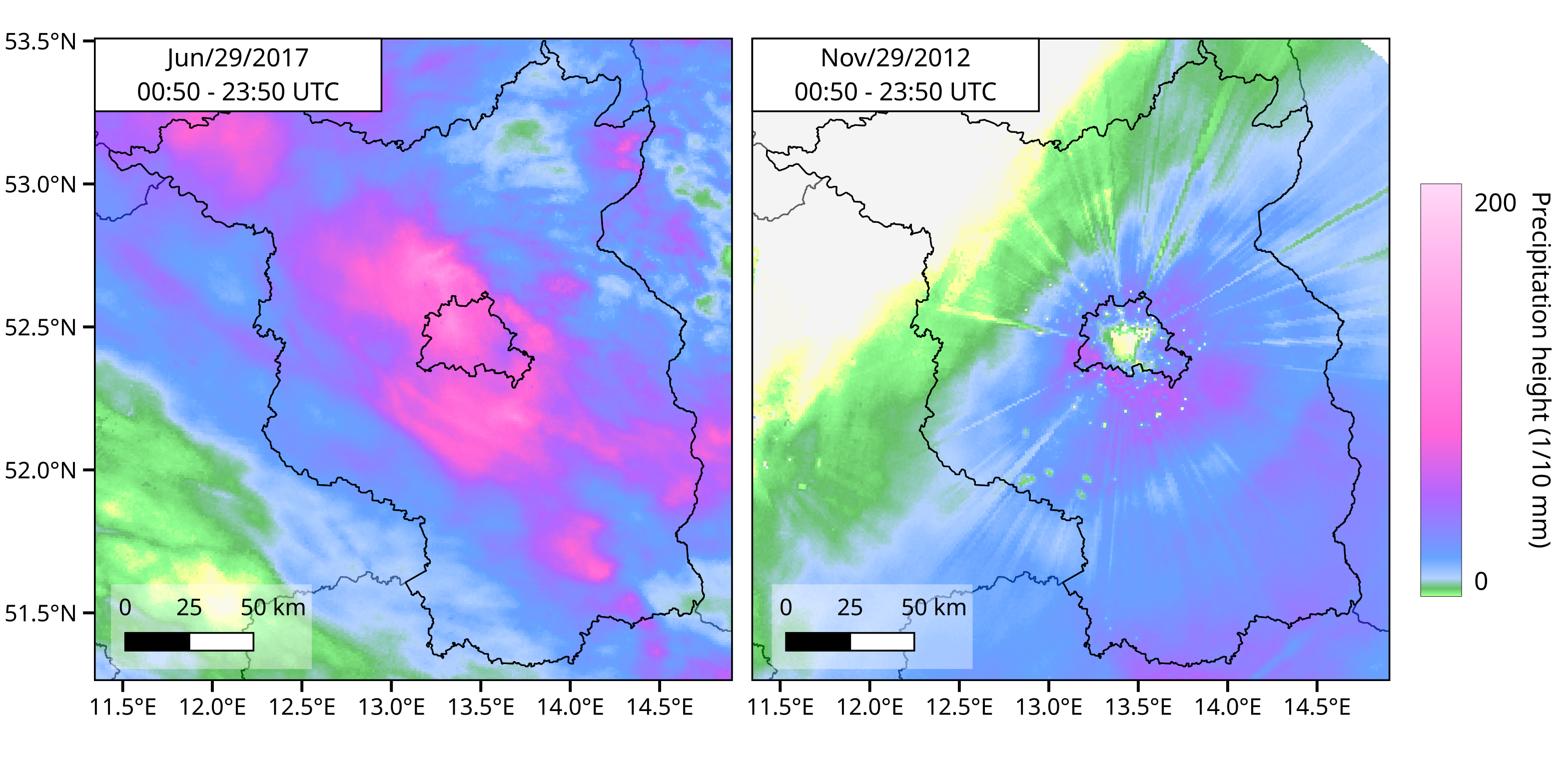
Figure 1: Map showing daily accumulated precipitation height for two extreme precipitation events chosen arbitrarily for demonstration). Left: A summer convective event. Right: A winter frontal event. Data comes from the RADOLAN database made available from the DWD.

In the midlatitudes region, the type of dominant rainfall-generating mechanism changes during the year. For example, Berg and Haerter (2013) found that synoptic observations of convective events dominated during the summer seasons in four stations across Germany. In contrast, they found that most rainfall in the winter months resulted from stratiform clouds (commonly associated with frontal events). Thus, we predict that when looking at seasonal block maxima for a study region in Germany, summer maxima will originate mainly from convective events, while winter maxima will primarily originate from frontal ones. An example of this can be seen in Fig. 1, which shows the daily precipitation height in the Berlin-Brandenburg region for a convective event in summer (left) against that of a frontal/stratiform event in winter (right). For most stations in the domain, the semi-annual block maxima in the two corresponding seasons were attained for these two particular events, meaning they can be seen as extreme events. Extremal dependence in space arises when an extreme event is large enough to impact several rain gauges simultaneously. Therefore, the extremal dependence heavily depends on the spatial characteristics presented by the rainfall generating mechanisms. Thus, if these mechanisms change seasonally during the year, we expect the dependence structure to also change throughout the year.

2 Methods and Data

In this study, we perform the statistical modeling of extreme rainfall using the block maxima approach. This approach is based on the Fisher-Tippett-Gnedenko theorem, which states that under mild conditions block maxima of a sufficiently large block length of independently and identically distributed random variables can be approximately modeled by the generalized extreme value (GEV) distribution. When dealing with rainfall, block lengths of one month have been proven to be long enough to assure convergence to the GEV distribution (Fischer et al., 2017). Yearly block maxima can then be used to fit the parameters of the GEV for each rain gauge individually, resulting in the “zeroth-order” approach to modeling extreme rainfall in space. This pointwise approach, however, does not pool any information across stations and, therefore, cannot predict values for ungauged sites. Prediction of ungauged sites can be achieved by extending the pointwise GEV approach to include spatial covariates, which pools information from different locations, typically resulting in reduced uncertainties for the estimated parameters of the GEV (Ulrich et al., 2020a). Nevertheless, this second approach ignores the spatial dependence in the data, resulting in a misspecified likelihood that consistently underestimates the uncertainty of the estimates. Our study extends this approach by using a max-stable process to include spatial dependence.

2.1 Data

We used accumulated hourly and daily precipitation height measurements (in mm) from 53 stations belonging to the German Meteorological Service (DWD) in the Berlin-Brandenburg region of Germany (Fig. 2). The data was acquired through the German Meteorological Service (DWD) Open Data Server using the R-package rdwd (Boessenkool, 2021). The stations were chosen to include only those that contained measurements with both hourly and daily periods. This choice reduced the available number of stations with daily measurements from 300 to 53. Reducing the total number of stations was considered necessary to ensure the fairness of the comparisons with results using stations with hourly measurements and to lower the computational burden needed to fit the models. The average distance between all station pairs was approx. 95 km, with a range of $[4,245]$ km. The raw data contains further information about the type of precipitation measured (liquid or solid), but for the purpose of this study no discrimination was done with regard to precipitation type.

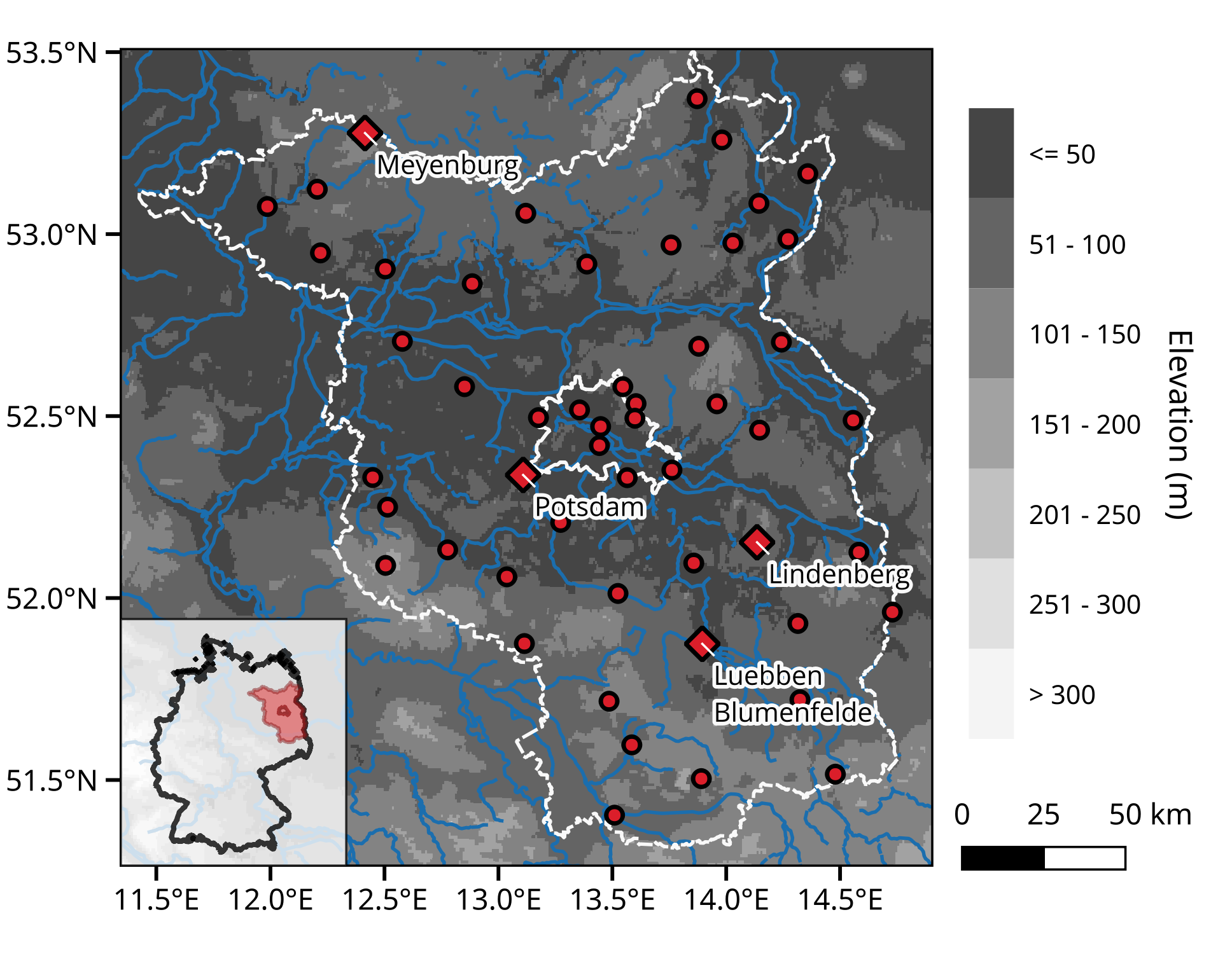
Figure 2: Map showing the location inside the Berlin-Brandenburg area of the DWD weather stations included in this study (red dots). The lower left inset shows the location of the study domain within Germany. Diamonds show the reference stations used to showcase results.

Two different periods were considered for this study: from 1970-2020 for the daily observations and 2004-2020 for the hourly observations. These periods were chosen in order to minimize the number of invalid pairs when using the pairwise likelihood (see Appendix A).

At the location $s_{j}\in\mathcal{S}$, where $\mathcal{S}$ represents the geographical domain and $j=1,...,n$ is an index denoting the rain gauge, the data contains the accumulated rainfall values $(r_{d,1}(s_{j}),...,r_{d,k_{j}}(s_{j}))$ in mm, where $d\in\{1,24\}$ is an index for the duration of the considered precipitation events, namely, hourly or daily. Different gauges can have different lengths for the measurement period, so that $k_{j}$ depends on the location $s_{j}$. The accumulated rainfall values were transformed to the average hourly/daily intensity values $(\zeta_{d,1}(s_{j}),...,\zeta_{d,k_{i}}(s_{j}))$ in mm/h.

Following (Koutsoyiannis et al., 1998), the average hourly intensity data $\zeta_{d=1,\tau}(s)$ (where $\tau$ represents the time (in hours) of the observation) were aggregated to create the 12-hour accumulated precipitation intensity time series $\zeta_{d=12,\tau}(s)$ (in mm/h). This aggregation was necessary because a visual inspection of the pairwise extremal coefficient resulting from the hourly series strongly suggested that the data was asymptotically independent, which violates a major assumption for using max-stable processes. The lowest aggregation duration that did not show asymptotic independence was 12 hours. The 12-hour aggregated series is obtained using

$$\zeta_{d=12,\tau}(s)=\frac{1}{12}\sum_{i=0}^{11}\zeta_{d=1,\tau-i}(s),$$ (1)

which can be seen as a moving average with a time window of 12 hours. The aggregation described in Eq. (1) was done using the package IDF (Ulrich et al., 2020b).

The 12-hour $\bm{\zeta}_{12}(s_{j})$ and daily $\bm{\zeta}_{24}(s_{j})$ average precipitation intensity series are then used to get four series of semi-annual block maxima series $(i_{d,t=1}^{l}(s_{j}),...,i_{d,t=N_{j}}^{l}(s_{j}))$. In this case, the index $t$ can be seen as indicating the year. These four series result from combining the two durations $d\in\{12,24\}$ and the two seasons $l\in\{\mathrm{sum},\mathrm{win}\}$ using the corresponding abbreviations for sumer and winter, respectively. The semi-annual block maxima were obtained using

$$i_{d,t}^{l}(s)=\max_{l_{t}^{-}<\tau<l_{t}^{+}}{\zeta_{d,\tau}(s)},$$ (2)

where $l_{t}^{-}$ and $l_{t}^{+}$ correspond to the beginning and end of either winter or summer for each year $t$. For this work, we consider summer as May, June, July, and August; winter is considered to be the months of January, February, November, and December. In order to avoid having winter block maxima that come from disconnected months, we shifted the $\bm{\zeta}_{d}(s)$ values of November and December to the following year, making the four winter months of any given calendar year come from the same “meteorological” winter. Note that for each instance of $\tau$ within the same type of season, i.e. summer or winter, and for each fixed duration $d\in\{12,24\}$, we perceive $\zeta_{d,\tau}(\cdot)$ as independent realizations of some stochastic process $\{X(s):\ s\in\mathcal{S}\}$ which will be the justification for the use of GEV distributions and max-stable processes for modeling the distribution of $i_{d,t}^{l}(s)$ below.

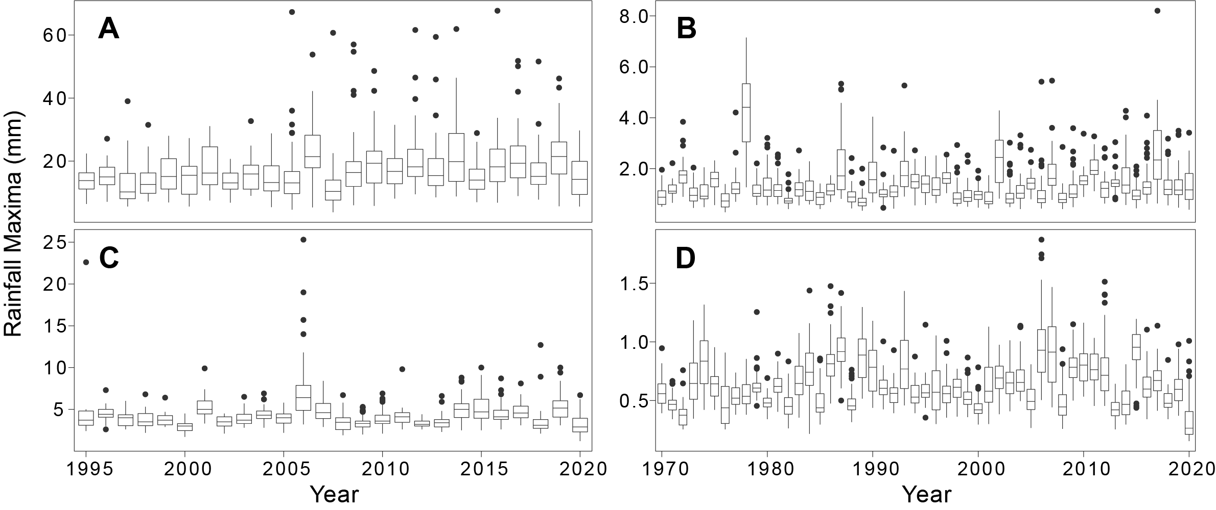
Figure 3: Boxplots showing the distribution of the rainfall semi-annual block maxima for the 53 stations included in this study. (A) 12-hour summer maxima, (B) daily summer maxima, (C) 12-hour winter maxima, and (D) daily winter maxima.

Figure 3 shows the temporal distribution of the semmi-annual block maxima for summer, i.e. $\bm{i}^{\mathrm{sum}}_{12}(s)$ and $\bm{i}^{\mathrm{sum}}_{24}(s)$, and winter, i.e. $(\bm{i}^{\mathrm{win}}_{12}(s)$ and $\bm{i}^{\mathrm{win}}_{24}(s))$ over the 53 stations. From Figure 3, it is apparent that the magnitude of the maxima changes depending on the season, with consistently larger values for summer events. The final length of the daily series is 50 years, while for the 12-hour series, it is 26 years.

2.2 Characterizing extremal dependence

To explore how the bivariate extremal dependence changes for the block maxima derived from the summer and winter seasons, we used an estimate of the empirical pairwise extremal coefficient $\theta(s_{j},s_{j^{\prime}})$, which is a summary measure of dependence of a random two-dimensional vector $(X(s_{j}),X(s_{j^{\prime}}))$ (Coles, 2001; Ribatet et al., 2016). The pairwise extremal coefficient can take values in the rage $[1,2]$, where 1 denotes complete dependence and 2 asymptotic independence.

For each pair $(s_{j},s_{j^{\prime}})$ of locations of gauged stations, we estimate the empirical extremal coefficient $\hat{\theta}_{\text{NP}}(s_{j},s_{j^{\prime}})$ using the non-parametric method proposed by Marcon et al. (2017), which (Vettori et al., 2018) found to have the best overall performance compared to other empirical estimators. The estimation of $\hat{\theta}_{\text{NP}}(s_{j},s_{j^{\prime}})$ is done with the R-package ExtremalDep (Beranger et al., 2021). This method requires the specification of a polynomial order, for which a graphical analysis (not shown) found that a fixed value of $k=20$ yielded the most appropriate values of $\hat{\theta}_{\text{NP}}(s_{j},s_{j^{\prime}})$ for the different $\bm{i}^{l}_{d}(s)$ series.

2.3 Modeling of extreme rainfall

We follow a two-step approach to model the $\bm{i}^{l}_{d}(s)$ series. In the first step, we model the marginal distribution of the pooled data from all stations by including spatial covariates within a Bayesian distributional model (DM). For the second step, we extend the model of the first step with a max-stable process, allowing the model to capture the so-called “residual dependence” left from the first-step that arises from the extremal dependence (Cooley et al., 2012). We then compare the models from both steps using a forecast verification framework to study how the extremal dependence influences the estimates of the model parameters. We consider the BDM approach to act as a “control” compared to the max-stable process approach, allowing us to explore how the seasonal difference in the extremal dependence affects the estimates down the line.

Estimations made within the framework of extreme value statistics are usually made with small data samples, as extreme events are by definition rare. The small sample size, in turn, leads to high uncertainty of all estimates, a problem compounded by the fact that most applications of EVT focus on the very far right of the distribution, where estimates already have high levels of uncertainty. Therefore, any EVT study must include information about the uncertainty that can be easily interpreted and adapted for the final-user applications. Uncertainty in this study is exclusively obtained using Bayesian methods for inference, which allow a straightforward and intuitive interpretation of their values.

The following sections explore the two approaches used for this study: First, the approach that includes spatial covariates but assumes independence in space (henceforth denoted as the DM approach), and second, the approach that uses a Brown-Resnick max-stable process to account for the spatial dependence (henceforth denoted as the BR approach).

2.3.1 Using a Bayesian distributional model

A simple but effective approach to model the variability of extreme rainfall in space is to pool information from all stations in the study region and assume that all values are independent and identically distributed. This approach assumes that observations at each station are independent of those at any other station. Instead, information is pooled from different stations using spatial covariates, such as the position of each station, as a predictor within a model. The resulting model can then characterize extremal behavior at unobserved locations simply by using their position in the covariates.

In this study, we use an analog of Vector Generalized Linear Models known in the Bayesian literature as Distributional Models (DMs), or sometimes, as Bayesian distributional regression (Umlauf and Kneib, 2018). Distributional models allow for the simultaneous linear modeling of all distributional parameters. This is in contrast to standard GLMs, where only the location parameter is modeled. Furthermore, like VLGMs, DMs allow the use of distributions from outside the exponential family, such as the GEV distribution. Extending a GLM to be a Bayesian DM is straightforward, as one requires only to add the additional log-likelihood contribution from the additional parameter models in the MCMC steps. Using these models, we can incorporate spatial covariates into linear models for every parameter of the marginal distributions.

For every rain gauge $j$ located at $s_{j}$, the block maxima $\bm{i}^{l}_{d}(s_{j})=(i^{l}_{d,1}(s_{j}),...,i^{l}_{d,N_{j}}(s_{j}))$ are assumed to be i.i.d. and, as the Fisher-Tippett-Gnedenko Theorem for block maxima suggests, follow the Generalized Extreme Value (GEV) distribution, which following (Coles, 2001) is given by

$$G(x)=\begin{cases}\exp\left[-\left(1+\xi\frac{x-\mu}{\sigma}\right)_{+}^{-1/\xi}\right]&\xi\neq 0,\\ \exp\left[-\frac{x-\mu}{\sigma}\right]&\xi=0,\end{cases}$$ (3)

where $\mu\in\mathbb{R},\sigma>0,\xi\in\mathbb{R}$ are the location, scale, and shape parameters, respectively, and $x_{+}=\max(0,x)$. This assumption is verified for all stations using Quantile-Quantile plots (not shown).

We then follow (Fischer et al., 2017) and describe the spatial variation of location $\mu$ and scale $\sigma$ using a linear combination of Legendre polynomials of longitude and latitude as covariates. Legendre polynomials form a set of orthogonal basis functions on $[-1,1]$, ensuring that their evaluations at the covariates – normalized to that interval – will be linearly independent. Our model is restricted only to the northing and easting coordinates, ignoring the altitude. Thus, we are left with the distributional model

$$\mu(s) =\beta_{0}^{\mu}+\sum_{j=1}^{J}\beta_{j,x}^{\mu}P_{j}(x^{\prime})+\sum_{k=1}^{K}\beta_{k,y}^{\mu}P_{k}(y^{\prime}),$$ (4)

$$\log(\sigma(s)) =\beta_{0}^{\sigma}+\sum_{j=1}^{J}\beta_{j,x}^{\sigma}P_{j}(x^{\prime})+\sum_{k=1}^{K}\beta_{k,y}^{\sigma}P_{k}(y^{\prime}),$$ (5)

$$\xi =\xi\,,$$ (6)

where $s=(x^{\prime},y^{\prime})$, and a logarithmic link function is used for the scale parameter $\sigma$ to ensure positivity. $P_{i}(\cdot)$ denotes the $i$th order Legendre Polynomial. We transform the coordinates from longitude and latitude to Universal Transverse Mercator (UTM) $x$ and $y$ coordinates (UTM zone 33N) so that the distances between stations are measured in meters instead of degrees, simplifying the analysis. The $(x,y)$ coordinates are then shifted and scaled to the $(x^{\prime},y^{\prime})$ coordinates within the $[-1,1]\times[-1,1]$ square in order to compute the respective Legendre Polynomials.

The shape parameter $\xi$ is left constant throughout the domain, as other studies have found that this parameter is complicated to estimate properly and can strongly impact the model’s performance (Cooley et al., 2012).

Model Selection

The linear model in Eqs. (4) and (5) requires an order for the Legendre Polynomials to be specified. The order is chosen within the model selection framework using the Widely Applicable Information Criteria (WAIC) (Vehtari et al., 2017). A total of 140 possible combinations of up to order $P_{5}(\cdot)$ were fitted, and the model with the lowest WAIC value was chosen. Furthermore, a regularizing prior (detailed below) was used to lower the risk of overfitting.

2.3.2 Using a max-stable process

For the second step of our study, we expanded the model for the marginal distribution presented in section 2.3.1 by a simple max-stable process. The latter was chosen to capture the extremal dependence in the rainfall maxima. Max-stable processes are extensions to infinite dimensions of finite-dimensional Extreme Value Theory models, arising as “the pointwise maxima taken over an infinite number of (appropriately rescaled) stochastic processes” (Ribatet, 2013).

More precisely, let $X(s)$ be a random variable representing the daily precipitation height at site $s\in\mathcal{S}$ (for some fixed duration $d$ and season $l$); that is $\{X(s):\ s\in\mathcal{S}\}$ is a stochastic process modeling the precipitation at each site in the spatial domain $\mathcal{S}$. If we have i.i.d. replicates $\{X_{i}(s):\ s\in\mathcal{S}\}$ of the process such as precipitation heights for different days within the same season, then as already discussed, under mild conditions, the Fisher-Tippett-Gnedenko Theorem states that, for each site $s$ and sufficiently large $n$, the distribution of $\max_{i=1,...,n}X_{i}(s)$ may be approximated by a GEV distribution with spatially varying parameters $\mu(s),\sigma(s),\xi(s)$. Assuming that not only the marginal distributions, but also the spatial dependence structures converge, by a spatial extension of the Fisher-Tippett-Gnedenko theorem the block maxima process $\{\max_{i=1,...,n}X_{i}(s):\ s\in\mathcal{S}\}$ can be approximated by a max-stable process $\{Z^{\prime}(s):\ s\in\mathcal{S}\}$, given that $n$ is large enough (Ribatet et al., 2016). Thus, max-stable processes does not only allow for arbitrary GEV marginal distributions $Z^{\prime}(s)\sim\mathrm{GEV}(\mu(s),\sigma(s),\xi(s))$, but also provide a flexible way of modeling the dependence structure of the maxima of the $X_{i}$ random fields.

Consequently, we will assume that the semi-annual block maxima $\bm{i}^{l}_{d}(s_{j})$ form realizations of a max-stable process $\{Z^{\prime}(s):\ s\in\mathcal{S}\}$ at the gauged sites $s_{j}\in\mathcal{S}$. It is common in extreme value theory to transform the original block maxima data $\bm{i}^{l}_{d}(s_{j})$ into standardized maxima $\bm{z}^{l}_{d}(s_{j})$ following unit Fréchet marginal distributions (i.e., the case where $\mu=\sigma=\xi=1$ in Eq. 3). Transformation of the margins to the unit Fréchet distribution does not affect the dependence structure. This transformation is performed via the relationship

$$z^{l}_{d,t}(s)=\left[1+\xi\left(i^{l}_{d,t}(s)-\frac{\mu^{l}(s)}{\sigma^{l}(s)}\right)\right]_{+}^{1/\xi}.$$ (7)

As this transformation can be easily reversed, it then allows us to focus on the max-stable process $\{Z(s):\ s\in\mathcal{S}\}$ without any loss of generality. For such standardized max-stable processes, a variety of parametric submodels has been developed including the popular Brown-Resnick max-stable process model (Kabluchko et al., 2009).

In our study, the marginal standardization requires the specification of response surfaces for $\mu^{l}(s)$ and $\sigma^{l}(s)$ to link $\bm{z}^{l}_{d}(s)$ to $\bm{i}^{l}_{d}(s)$. We chose the response surfaces to have the same expressions as the model resulting from the model selection of Eqs. (4) and (5), with the shape parameter assumed to be constant over the entire domain.

In theory, max-stable process models can be used to model the joint distribution of all semi-annual block maxima $(i^{l}_{d,1}(s_{j}),\ldots,i^{l}_{d,N_{j}}(s_{j}))$, $j=1,\ldots,53$, and their standardized analogues $(z^{l}_{d,1}(s_{j}),\ldots,z^{l}_{d,N_{j}}(s_{j}))$, $j=1,\ldots,53$, respectively. In practice, however, the resulting likelihood terms are intractable for even relatively low-dimensional settings. This is why a common strategy is to restrict the process to the bivariate case, where the distribution functions and their corresponding densities are well-known. The bivariate joint probability for the rescaled maxima $Pr\{Z^{l}_{d}(s)\leq z_{1},Z^{l}_{d}(s+\bm{h})\leq z_{2}\}$ is then modeled using the bivariate distribution of the Brown-Resnick max-stable process model (Kabluchko et al. (2009), see appendix A). For the Brown-Resnick model, the extremal spatial dependence is a function only of the variogram $\gamma$, which, with a slight abuse of notation, for this study has the following theoretical model:

$$\gamma(s,s+\bm{h})=\gamma(\bm{h})=\left(\frac{\|\bm{h}\|}{\rho}\right)^{\alpha},$$ (8)

Here, $\|\bm{h}\|$ is the Euclidean distance between the two locations considered, $\rho$ is the range parameter, and $\alpha$ is the smoothness parameter. The range parameter $\rho$ can be seen as the distance for which the dependence is still effective and takes values $(\rho>0)$. The smooth parameter $\alpha$ has no straightforward interpretation and is constrained to be $\alpha\in[0,2]$. For this study, we restrict the variogram to be isotropic and stationary, i.e. $\gamma(s,s+\bm{h})$ depends on $\|\bm{h}\|$ only. The two Brown-Resnick parameters $(\alpha,\rho)$ contain the information regarding the pairwise dependence structure. To compare the Brown-Resnick dependence estimated from the model with the empirical dependence shown by the data, we also obtain a parametric estimate of the bivariate extremal coefficient $\theta(s_{j},s_{j^{\prime}})$ using the $(\rho,\alpha)$ parameters of the Brown-Resnick model. This parametric estimate $\theta_{\mathrm{BR}}(s_{j},s_{j^{\prime}})$ is computed from the Brown-Resnick variogram $\gamma(h)$ obtained in Eq. (8) using the following relationship:

$$\theta_{\mathrm{BR}}(s_{j},s_{j^{\prime}})=2\Phi(\gamma(\|s_{j}-s_{j^{\prime}}\|)/2)^{1/2}),$$ (9)

where $\Phi$ represents the standard normal distribution function.

2.3.3 Statistical Inference

The estimation of the posterior distribution of the $(\beta_{0},\beta_{i,P})$ coefficients for the DM approach and the response surfaces, as well as for the BR dependence parameters $(\alpha,\rho)$, was carried out using Bayesian inference. Given a random variable or vector $Y$ and a probabilistic distribution function $G(\phi)$ such that one assumes that $Y\sim G(\phi)$ (where $\phi$ represents the distributional parameters), Bayesian inference assumes that the parameters $\phi$ also follow a probability distribution. The quantity of interest is the so-called posterior distribution of probable values for $\phi$ given observations $y$ from the random variable $Y$, which is obtained using Bayes’ rule: $p(\phi\mid y)\propto p(y\mid\phi)p(\phi).$ The uncertainty of the estimates is then directly obtained from the posterior distribution $p(\phi\mid y)$. Furthermore, the likelihood $p(y\mid\phi)$ is derived from the model, and has the same mathematical expression as the likelihood used for MLE methods. Finally, the so-called prior $p(\phi)$ includes the information known about the parameters $\phi$ before observing the data $y$. For studies involving extremes, the choice of $p(\phi)$ is of particular importance, as the small size of the data sample typically results in a strong influence of the prior over the posterior. (Stephenson, 2016) provides current strategies to choose appropriate priors when performing inference of the GEV distribution.

For the inference of the parameters in this study, we used a Markov Chain Monte Carlo (MCMC) sampling scheme. MCMC sampling requires that the right-hand side of Bayes’ rule is known up to a multiplicative constant, for which it is enough to know the expression for the likelihood $p(Y\mid\phi)$ and the prior distribution $p(\phi)$.

The likelihood term of the DM approach given by Eqs. (4)-(6) is directly obtained from the GEV distribution (Eq. (3)). For the BR approach, using the full likelihood is unfeasible as the data’s high dimensionality made the full likelihood intractable; we chose instead to use the pairwise likelihood from (Padoan et al., 2010) (see Appendix A for details). The expression for the pairwise likelihood of the Brown-Resnick model included both the marginal and dependence parameters so that each MCMC step updated the value of all $\phi=\{\rho,\alpha,\beta_{0}^{\mu},\beta_{0}^{\sigma},\beta_{0}^{\xi},\beta_{i,P}^{\psi}\}$ parameters simultaneously, where $\beta_{i,P}^{\psi}$ denotes all potential relevant coefficients for $\psi=\left\{\mu,\sigma\right\}$ aside from their intercepts $\beta_{0}^{\mu}$ or $\beta_{0}^{\sigma}$.

The last step to perform Bayesian inference is to propose a prior distribution for all parameters. For the DM approach, this includes the three intercepts $(\beta_{0}^{\mu},\beta_{0}^{\sigma},\beta_{0}^{\xi})$ and all the possible coefficients $\beta_{i,P}^{\psi}$, where $\psi\in\{\mu,\sigma\}$.

The covariates were recentered around zero so that the value of the intercepts can be interpreted as the value when all other covariates are set to their mean values. Based on the study of (Fischer et al., 2017), who did a similar analysis for the same region, we use the following priors for the location and scale intercepts:

$$\beta_{0}^{\mu} \sim\mathrm{Normal}(1.54,0.6166)$$ (10)

$$\beta_{0}^{\sigma} \sim\mathrm{Normal}(0.4166,0.4166)$$ (11)

The prior for the shape parameter $\xi$ is a rescaled Beta-distribution $\beta_{0}^{\xi}\sim\mathrm{Beta}(2,2)$ that has support in $[-0.5,0.5]$. This choice was made as this prior has already been used by Dyrrdal et al. (2015) and also in the operational application used by MeteoSwiss (Fukutome et al., 2018). For the $\beta_{i,P}^{\psi}$, we use the prior $\beta_{i,P}^{\psi}\sim\mathrm{Student-t}(2,0,1)$, which is a regularizing prior (Kruschke, 2014), preventing overfitting.

For the BR approach, the priors for the marginal response surfaces were the same as those used for the DM approach described above. Using the same priors for the two models was done to simplify the comparison between them. Additionally, the prior for the range parameter $\rho$ and the smooth parameter $\alpha$ were elicited from typical values of these parameters in other studies (Zheng et al., 2015; Stephenson et al., 2016) and were chosen to be $p(\rho)=\mathrm{Normal}(30000,7000)$ and $p(\alpha)=\mathrm{Exponential}(2.5)$, respectively. The scales of the parameters for $p(\rho)$ are in meters.

MCMC sampling was performed using the software Stan (Stan Development Team, 2022). A total of 4 chains with 2500 post-warmup samples per chain using 1000 samples as warmup was used. A visual analysis of the ridge and trace plots was performed for all models to detect issues with MCMC chain convergence.

A known issue when using pairwise likelihoods for Bayesian inference is that the resulting posterior distributions will severely underestimate the spread of the distribution ((Ribatet et al., 2012, 2016; Chan and So, 2017)). The underestimation occurs because the pairwise likelihood over-uses the data by including each location in $n/2$ terms of the objective function rather than just one, as would be the case with the full likelihood, resulting in a likelihood function that is far too sharply peaked (Ribatet et al., 2012). While this issue does not severely affect the overall median of the posterior distribution (Chan and So, 2017), the estimated credible intervals of the parameters will be strongly underestimated. To tackle this issue, we applied the Open Faced-Sandwich (OFS) correction proposed by (Shaby, 2014) to all posterior MCMC samples from the Brown-Resnick model. The OFS-corrected samples produce credible intervals that have proper coverage values. However, it is worth noting that while the resulting posterior samples fulfill the desired coverage properties, they are no longer truly Bayesian. Appendix C shows a comparison between the raw MCMC samples and the OFS-corrected ones.

2.3.4 Prediction of return levels

Once a posterior distribution of the marginal GEV parameters is obtained from the MCMC samples, it is straightforward to calculate $q_{p}(s)$ quantile levels for any probability $p$ of non-exceedance (i.e., return levels) via the quantile function of the GEV distribution

$$q_{p}(s)=\begin{cases}\mu+\frac{\sigma}{\xi}[(-\log p)^{-\xi}-1]&\xi\neq 0,\\ \mu-\sigma\log(-\log p)&\xi=0\,.\end{cases}$$ (12)

For each one of the $S$ MCMC sampled parameter values, we calculate a value of $q_{p}(s)$ with probability $p$. This results in a distribution of $S$ return levels. We report the median of these return levels as the estimated return level. Their uncertainty is calculated as the $2.5\%$ and $97.5\%$ quantiles of the $S$ return levels, forming $95\%$ credibility intervals. Note that the resulting return levels no longer stem from a GEV distribution but rather from a mixture of many GEV distributions.

2.4 Verification and Model Comparison

We use the quantile score (QS) (Bentzien and Friederichs, 2014) as a measure of accuracy for both the marginal and the Brown-Resnick models. Given a series for a single rain gauge of semi-annual block-maxima observations $(i^{l}_{d,1}(s_{j}),...,i^{l}_{d,N_{j}}(s_{j}))$ with $N_{j}$ years of data for the $j$-th gauge and the corresponding prediction for the quantile level $q^{l}_{p,d}(s_{j})$ with probability $p$ for the same location $s_{j}$, duration $d$ and season $l$, the QS is defined as:

$$QS^{l}_{p,d} =\frac{1}{N}\sum_{t=1}^{N}\rho_{p}(i^{l}_{d,t}(s_{j})-q^{l}_{p,d}(s_{j}));$$ (13)

$$\mathrm{where}\quad\rho_{p}(u)=[\lvert u\rvert+(2p-1)u]/2.$$ (14)

The QS is always positive and reaches an optimal value at zero. We obtain the QS values for both the marginal and the Brown-Resnick model for probability levels of $p=(0.9,0.95,0.98,0.99)$, corresponding to return periods of $(10,20,50,100)$ years.

To compare the performance of two models, Ulrich et al. (2020a) defined the Quantile Skill Index (QSI), a measure derived from the Quantile Skill Score QSS (cf. Wilks, 2011, for an introduction to skill scores). Given the QS for a model to be tested ($\mathrm{QS}_{\mathrm{model}}$) and the QS for a reference model $(\mathrm{QS}_{\mathrm{ref}})$, the QSI is defined as

$$\mathrm{QSI}=\begin{cases}1-\frac{\mathrm{QS}_{\mathrm{model}}}{\mathrm{QS}_{\mathrm{ref}}},&\mbox{if }\mathrm{QS}_{\mathrm{model}}<\mathrm{QS}_{\mathrm{ref}}\\ -\left(1-\frac{\mathrm{QS}_{\mathrm{ref}}}{\mathrm{QS}_{\mathrm{model}}}\right),&\mbox{if }\mathrm{QS}_{\mathrm{model}}\geq\mathrm{QS}_{\mathrm{ref}}\end{cases}\,.$$ (15)

Positive (negative) values of the QSI indicate a gain (loss) of skill for the tested model over the reference. The advantage of the QSI over the QSS is that the interpretation of negative or positive values is equivalent (which is not the case for skill scores). For this study, the tested model is the Brown-Resnick max-stable process model, and the reference model is the marginal distributional model.

To get an estimation of the out-of-sample performance for the QSI, we applied 10-fold cross-validation in space to estimate the QS values. The folds were constructed such that in each one, 90% of the stations were used for training the model and the remaining 10% for validation. Each station appears in a given validation set once and only once. This specific cross-validation scheme gives an estimate of how good the model is at predicting values at ungauged sites, and it does not give any information on the model’s skill at predicting future observations. Considering the sizeable computational load needed to perform MCMC sampling for all 8 models for all 10 folds, we opted to use maximum likelihood instead of Bayesian inference for this step. Using MLE instead of full Bayesian inference was considered a fair assessment as we are only interested in point estimates of return levels when calculating the QS using Eq. (14). A separate analysis (not shown) revealed that the QS point estimates obtained from maximum likelihood were almost always very similar to the median QS values obtained from the full posterior distribution.

3 Results

3.1 Extremal dependence

The estimated bivariate extremal coefficient $\hat{\theta}_{\text{NP}}(s_{j},s_{j^{\prime}})$ for the $\bm{i}^{\mathrm{(sum,win)}}_{12}(s_{j})$ and the $\bm{i}^{\mathrm{(sum,win)}}_{24}(s_{j})$ block maxima series is shown in Fig. 4. The main feature is that winter maxima (blue) consistently show lower average values (i.e., higher extremal dependence) until a distance of around $h=150$ km. For distances $h>150\mathrm{km}$ this relationship is inverted. Furthermore, the average distance where the pairwise maxima still show asymptotical dependence is shown to be lower than 150 km. The difference between seasons is larger for the 12-hour series, possibly reflecting differences in the rainfall generating mechanisms at this timescale compared to the 24-hour series.

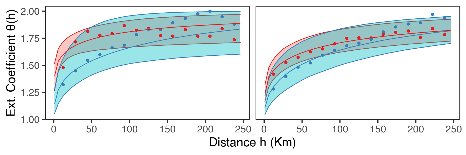
Figure 4: Empirical values of the extremal coefficient $\hat{\theta}_{\text{NP}}(s_{j},s_{j^{\prime}})$ (dots) and estimated values from the resulting Brown-Resnick variogram $(\theta_{\mathrm{BR}}(s_{j},s_{j^{\prime}})$ (solid lines, shaded regions represent the 50% CI). Colors represent the season: blue for winter and red for summer. The left panel shows results from the 12-hourly data; the right panel shows results for the daily data. $\theta(s_{j},s_{j^{\prime}})\in[1,2]$, where one is complete dependence and two is complete independence.

Estimates of the extremal coefficient based on the Brown-Resnick model ($\hat{\theta}_{\mathrm{BR}}(s_{j},s_{j^{\prime}})$) are also shown in Fig. 4 as the solid lines with the shaded regions representing 50% credibility intervals. We compare the values from the Brown-Resnick model to the empirical $\hat{\theta}_{\text{NP}}(s_{j},s_{j^{\prime}})$ to get an idea of how well the BR approach captures the pairwise dependence shown by the data. For the 12-hour series (left), this comparison shows that for winter, the model consistently overestimates the strength of the dependence for $h>100$, while for summer, the average dependence is properly captured for $h\lesssim 150$ km; for greater distances, the dependence is underestimates. The overestimation in the winter model can also be seen for the daily series (right); however, it is much less pronounced, with most of the average $\hat{\theta}_{\text{NP}}(s_{j},s_{j^{\prime}})$ falling inside of the 50% CIs. In both time series, the 50% CIs are larger for winter; this could suggest that the extremal dependence for winter is more complex than for summer, resulting in the winter model exploring a greater range of values for the dependence parameters. Additionally, the daily series shows less variability than the 12-hour series. This difference in variability may be due to the increased length of observations for the daily series.

An initial inspection of the $\hat{\theta}_{\text{NP}}(s_{j},s_{j^{\prime}})$ values would suggest that the data shows asymptotic dependence for all series for distances up to $h\leq 150$ km. Therefore, the assumption of asymptotic dependence necessary for using a max-stable process, should be justified. Further discussion about this topic can be found in Appendix D.

3.2 Model building

3.2.1 Model selection

The procedure to choose the orders for the Legendre Polynomials of Eqs. (4)-(6) results in the models described in Tab. 1. Basic prior and posterior predictive checks were performed to detect any misspecification issues; some examples for the reference stations described below can be found in Appendix E. A visual analysis of the prior and posterior checks did not detect any severe issues.

Table 1: Maximum chosen orders of Legendre Polynomials for the distributional model in Eqs. (4)-(5)

. $\mu$ $\sigma$ summer (24h) 2 1 winter (24h) 3 2 summer (12h) 2 1 winter (12h) 3 2

3.3 Parameter estimates

Parameter estimates for the dependence and shape parameters are reported in Tab. 2 as median and 95% credibility intervals for each parameter. A distinct difference can be seen in the value of the range parameter $\rho$ (in meters) between summer and winter, as the value in winter is always significantly larger than for summer, regardless of the time scale. This result is consistent with the behavior of the extremal coefficient seen in Fig. 4, and it may indicate that the rainfall events leading to the block maxima in winter are, on average, larger than those in summer. Furthermore, the shape parameter shows a difference for winter and summer, regardless of the time scale.

Table 2: Bayesian estimates of the Brown-Resnick max-stable model parameters. Posterior medians are reported along with their 95% credible interval limits on either side as (lower,median,upper). The coefficients corresponding to the Legendre Polynomials were omitted from this table.

	$\rho$	$\alpha$	$\xi$
12h (s)	413,4896,11997	0.17,0.40,0.64	0.05,0.18,0.31
12h (w)	3596,43870,104192	0.31,0.78,1.24	-0.01,0.08,0.20
24h (s)	4722,22993,43936	0.39,0.54,0.69	0.15,0.24,0.33
24h (w)	6801,53228,109265	0.57,0.83,1.12	-0.01,0.09,0.21

3.4 Marginal parameters and return levels

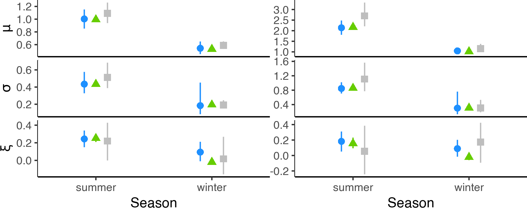
Figure 5: Estimated values of the location $\mu$, scale $\sigma$, and shape $\xi$ parameters of the GEV distribution for station Potsdam. The symbols’ shape indicates the model used for estimation: circle (blue) = BR, triangle (green) = DM, square (gray) = pointwise GEV.

Four reference stations were chosen to illustrate the differences in the marginal GEV parameters and return levels from the DM and the BR models (respective locations of the reference stations are given by red diamonds in Fig. 2). We chose the two stations with the longest time series, which are closely surrounded by other stations (Potsdam and Lindenberg), a station with a long time series that is isolated from other stations (Meyenburg), and a station with a short time series which is surrounded by other stations (Luebben-Blumensfelde). Figures 5-6 show the GEV parameter estimates and the resulting return levels with 95% credibility intervals, respectively. Furthermore, pointwise GEV estimates and their resulting return levels with 95% credibility intervals were added for reference; these estimates were obtained using the same priors for the intercepts described in section 2.3.3.

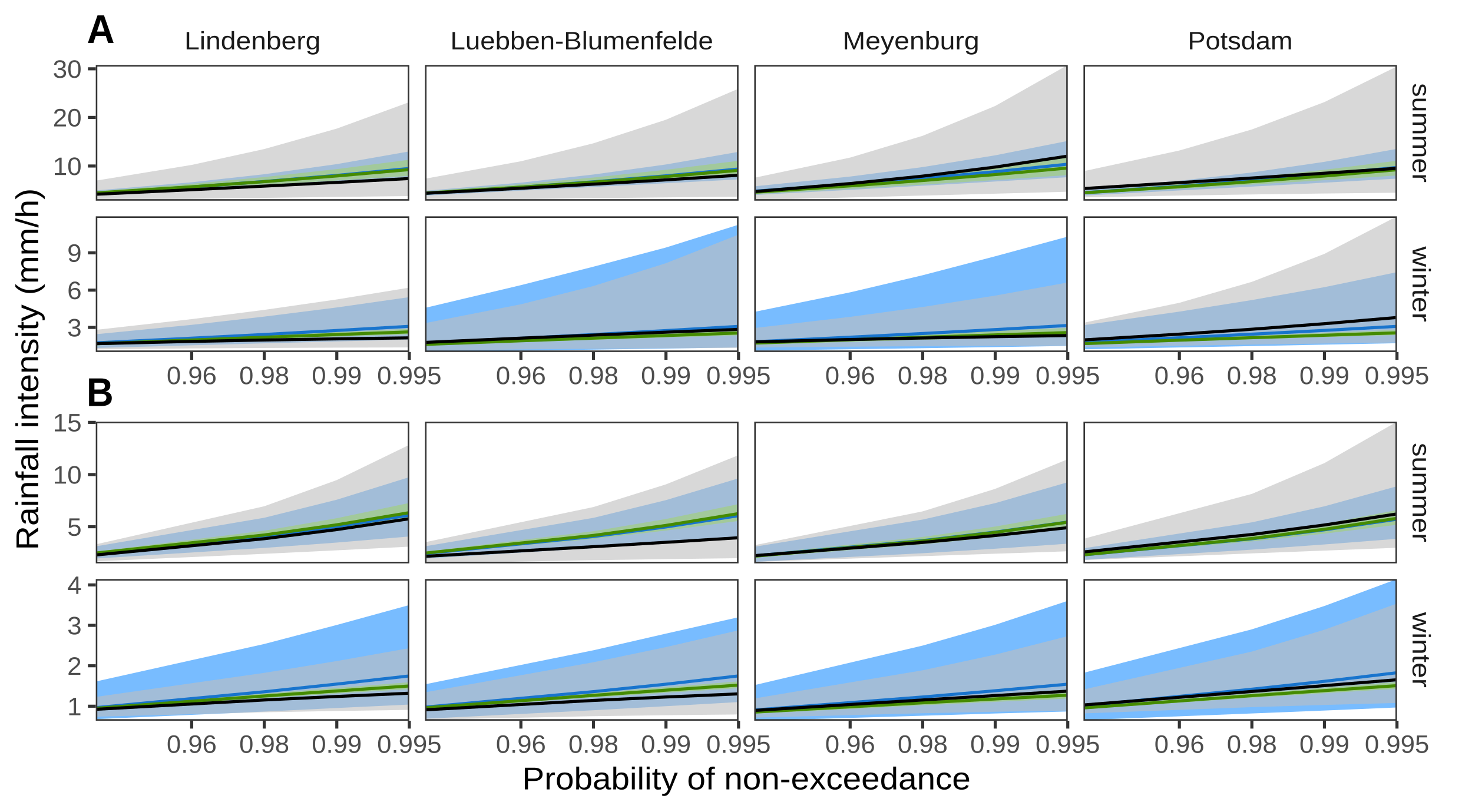
Figure 6: Return level of precipitation intensity (mm/h). Color denotes the model used: Blue for the BR model, green for the DM model, and gray for the pointwise GEV. Shaded regions represent pointwise 95% credibility intervals. (A) 12-hour data, (B) daily data. For reference, the probabilities of non-exceedance $p=(0.96,0.98,0.99,0.995)$ correspond to the $(25,50,100,200)$ year return periods, respectively.

Concerning the GEV parameters, Fig. 5 shows that the pointwise estimates (taken here as the median value of the posterior distributions) are similar for the DM and the BR models. This similarity was expected, as the marginal parameters are only vaguely affected by the spatial dependence through their incorporation in the likelihood term of Eq. (16). However, when comparing the models, a pattern concerning the uncertainty of the estimated parameters (taken here to be the 95% credibility intervals) is visible. For summer (and in the case of $\xi$, also winter), the highest uncertainty is always seen for the pointwise GEV model, followed by the BR model and the DM model, which consistently show the smallest uncertainty. In contrast, the largest uncertainty for location and scale in winter can be seen for the BR model, followed by the pointwise GEV and the distributional models. This phenomenon can be observed in other stations (not shown). We infer that the uncertainty estimated for the marginal parameters is strongly affected by the underlying spatial dependence, which changes according to the rainfall-generating mechanisms dominant in the respective season.

To further delve into the last point, Fig. 6 presents how the return levels for different non-exceedance probabilities for the BR and DM approaches differ. As before, we compare different seasons and two different durations. The median return level is generally similar across the different models, with increasing differences for larger probabilities of non-exceedance. In contrast, the uncertainty is noticeably different for each model, which is consistent with the results of the GEV parameters. In summer, the uncertainty is always largest for the pointwise GEV model, followed in order by the BR and the DM models. This changes in winter, when the uncertainty is largest typically for the BR model, with a few exceptions. Surprisingly, it would appear that the inclusion of the max-stable dependence on the model for winter resulted in an overall increase in the uncertainty, even when compared to the pointwise model that contains no information about other stations. This result may be associated with a loss of skill for the BR model when modeling block maxima in winter, an aspect that will be explored in the next section.

3.5 Model comparison

We now explore how the seasonal differences in the extremal dependence affect the accuracy of the return levels estimates using the BR model. We use the DM approach as reference in the QSI to assess how much the dependence influences the return level estimates. Positive (negative) QSI values mean that the predicted return levels for ungauged sites have better (worse) QS values for the dependent BR model than for the independent DM one. For this study, our main focus is on the QSI difference between seasons, as we believe this arises from a change in the extremal dependence when analyzing the semi-annual block maxima from different meteorological regimes.

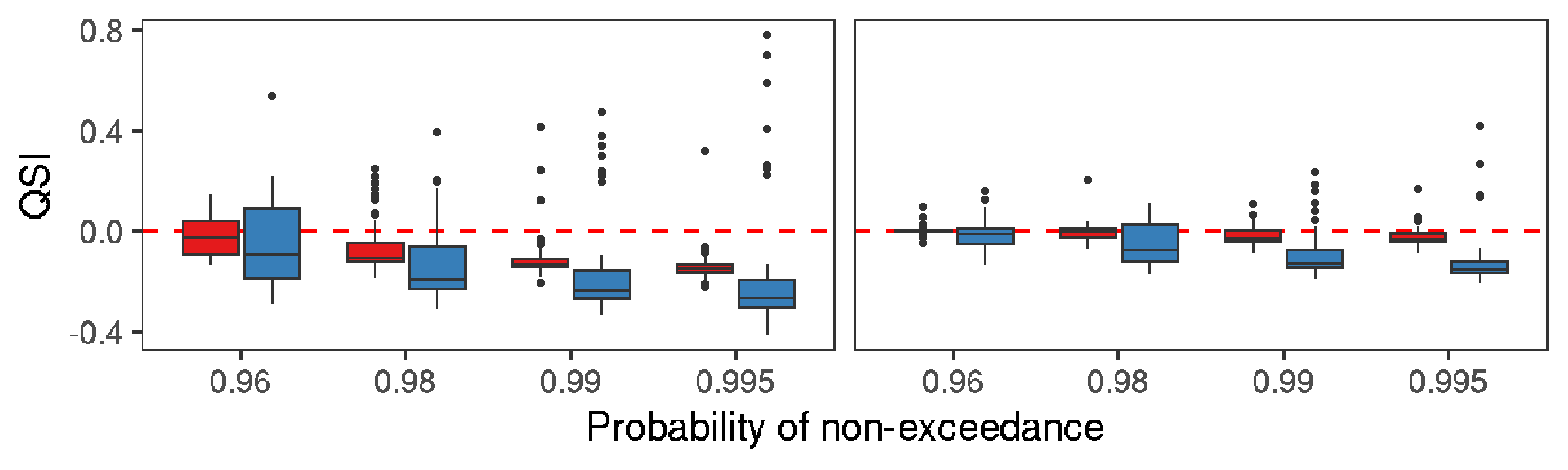
Figure 7: Boxplots showing the distribution of the Quantile Skill Index for all stations for 12-hourly (left) and daily (right) data. The colors indicate the season. Positive (negative) values indicate an increase (decrease) in skill for the BR approach compared to the DM one.

Figure 7 depicts the distribution of the cross-validated QSI values over all stations. The 12-hourly data shows an overall average loss of skill for the winter and summer models when using the BR model. This loss of skill increases as the non-exceedance probability increases, with the winter model showing substantially lower average QSI values than the summer model. Furthermore, the variability in QSI values is noticeably larger for winter than summer; in fact, the highest QSI value is always found within an outlier of the winter model. For the daily data, the winter model shows the same decrease in skill with increasing non-exceedance probabilities with high variability; however, in this case, the summer model consistently shows QSI values close to zero with very low variability. Finally, a noteworthy difference between average QSI values can be observed between summer and winter for both periods. This difference increases with the non-exceedance probability, but it remains constant between the 12-hourly and daily periods.

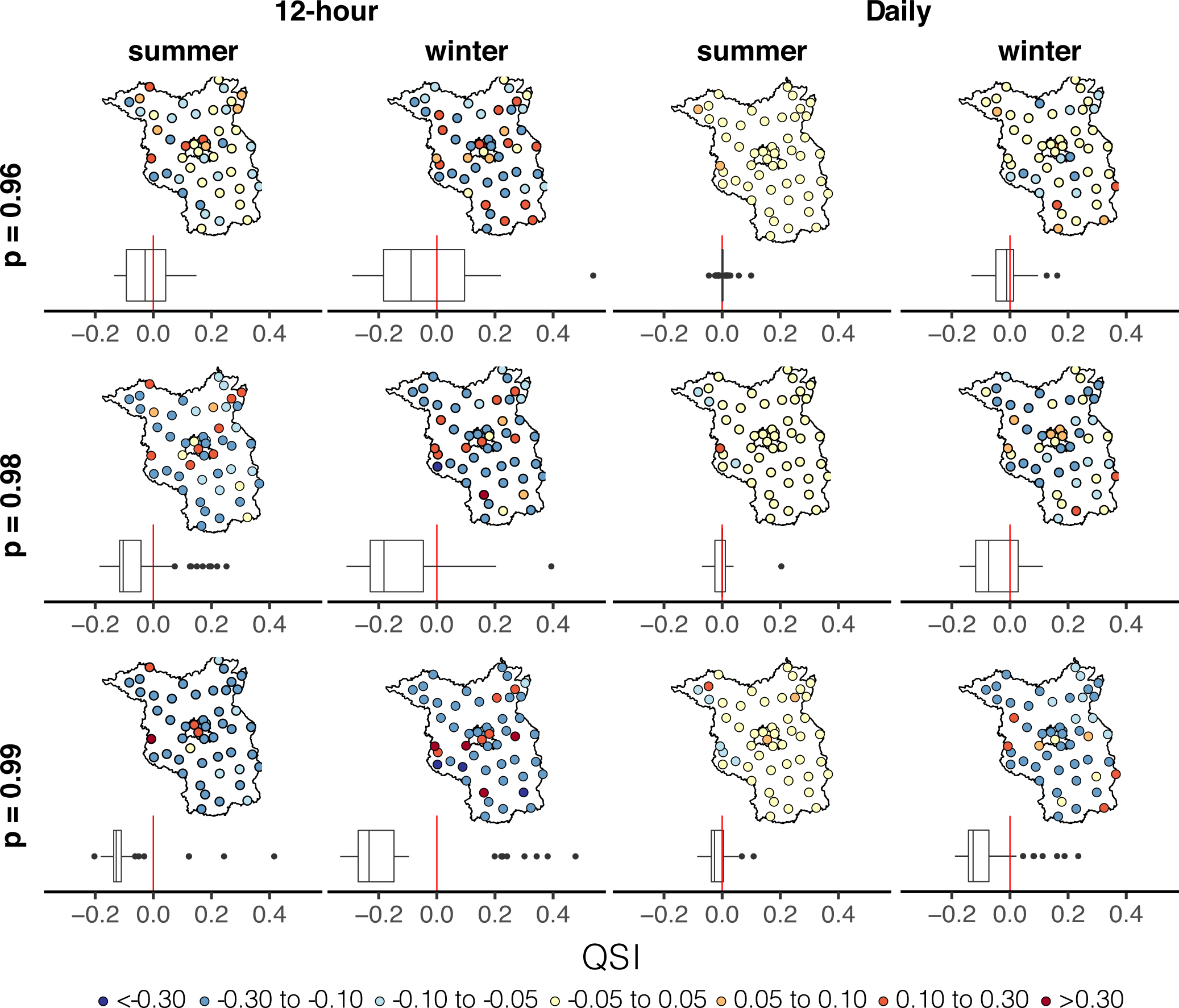
Figure 8: Spatial distribution within Berlin-Brandenburg (solid line) of QSI values for the 12-hourly (leftmost two columns) and daily (rightmost two columns) data. Boxplots below each map show the distribution of QSI values as in Fig. 7

To further explore the difference in QSI values for both seasons and durations, Figure 8 shows the spatial distribution of QSI values, i.e. values for every station. No apparent pattern is visible from the different configurations, as QSI values appear to be largely random. Nevertheless, the lowest QSI appear mostly at stations close to the domain’s border, suggesting that the BR model performs better when a station is surrounded on all sides by other stations. This effect is admittedly not very reliable, as stations with very low values of QSI can also be found within the middle of the domain. A closer inspection of the difference between seasons reveals a subtle pattern: similar QSI values seem to cluster in summer, while the distribution is predominantly random in winter. This change could be attributed to the difference in the rainfall generating processes, as will be discussed in the following.

4 Discussion

The results described in the last section provide compelling evidence that the extremal dependence shown by the data changes sufficiently enough to have a noticeable effect in the resulting marginal estimates down the line when using a model capable of capturing such dependence (the BR model in our case). This difference was mainly observed when comparing different marginal quantities from two seasons: the estimated GEV parameters (with their respective return levels) and the cross-validated Quantile Score (QS), an out-of-sample performance measure for the predicted return levels for ungauged sites.

The observed difference in marginal estimates when using a spatial model is consistent with previous extreme rainfall studies; Stephenson et al. (2016), for example, reports that the incorporation of the max-stable process dependence led to an overall shift towards heavier tailed marginal distributions across their study location. They also found that the uncertainty for the estimated marginal quantities was larger for the max-stable process model than for the independent model, which is in good agreement with our results for summer maxima estimated return levels. Additionally, the spatial distribution of the QSI falls in line with Le et al. (2018), who found that return levels estimated from a max-stable process presented noticeable differences in their spatial distributions compared to an unconditional model. However, these studies did not estimate the impact of this difference on the model performance. Our study then provides insight into the operational use of Brown-Resnick max-stable models by first examining how different types of rainfall-generating mechanisms affect the marginal estimates and then applying a model validation framework for the out-of-sample ungauged model accuracy.

A comparison of the uncertainty in the GEV parameters and the return levels showed that when modeling summer maxima, the uncertainty resulting from the BR model appeared to be a middle point between the DM and the pointwise GEV models. However, the significant reduction in uncertainty for the DM model compared to the pointwise GEV model signals that this model underestimates the natural variability in the rainfall data. Thus, it seems plausible that the larger uncertainty seen in the BR model is a more accurate representation of such variability. In contrast, when dealing with winter maxima, the uncertainty obtained by the BR model appears to have been consistently overestimated compared to the pointwise approach. From our results, it is not completely clear why this is the case, but it may be speculated that the isotropic Brown-Resnick dependence model was misspecified for the extremal dependence structure in the winter data. A possible source of error is the assumption that the dependence structure is isotropic, which might be a better approximation for convective events than for synoptic/mixed events that occur in winter. On the other hand, the larger values estimated for the range and smooth parameters indicate that the dependence is stronger for winter than in summer; however, these parameters do not say anything about the isotropic/anisotropic structure. This larger dependence in winter could be attributed to frontal events being generally larger and more elongated than convective events. Thus, more stations are simultaneously affected by the same event, increasing the dependence. Figure 9 in appendix D reports how many unique events resulted in block maxima being chosen from the daily series in winter and summer. This table supports the idea that the events are larger in winter, as the number of unique events is consistently lower in winter than in summer. However, Fig. 4 also reveals a surprising increase in dependence for distances larger than 120 km; this may suggest that some underlying weather patterns from a larger scale than the convective scale influence the dependence.

Our findings report that the Brown-Resnick model is mostly as good as the unconditional DM model when modeling summer block maxima, whereas the BR model presents a remarkable loss in skill compared to the DM model when modeling winter block maxima. It is worth noting that past studies have primarily focused on summer maxima, as the convective nature of the rainfall-generating mechanisms in this season typically leads to the annual maxima events to occur in summer. Our findings suggest that the isotropic Brown-Resnick dependence model is a proper first approximation when dealing with block maxima resulting from convective events. On the other hand, the loss in skill for the winter maxima model provides further evidence that this model is misspecified when dealing with either synoptic, stratiform, or a mixture of synoptic/convective events.

We acknowledge potential limitations to this study. An important question for future studies is to determine the effect of anisotropy in the results, which, as discussed above, is expected to have an important role in modeling the spatial dependence for synoptic events. Furthermore, previous studies have shown that rain gauge networks are typically too scarce to resolve convective cells properly (Lengfeld et al., 2019). Thus, in order to get a better representation of the spatial dependence, future work should make use of radar networks to complement rain gauge data. A significant limitation of our work was the use of the pairwise likelihood instead of the full likelihood of the Brown-Resnick model within the Bayesian framework. While some of the most known issues with this approach were tackled by using the Open-Faced Sandwich approach of (Shaby, 2014), it would be beneficial instead to use a full-likelihood approach such as that of (Dombry et al., 2017). Furthermore, due to the high computational demand of performing Cross-Validation within a Bayesian setting, the QS and QSI results reported in the results come from a maximum likelihood estimation. Moreover, we assumed that the data was stationary, ignoring the possible effects of climate change. The effect of this non-stationarity on the extremal dependence should be explored in further studies, as it has been shown that accounting for non-stationarity results in a measurable effect on the return level estimates (Ganguli and Coulibaly, 2017). Our study indirectly classified precipitation types based on dominant types for different seasons. Further studies should use a direct classification of event types, which would avoid the mixing of convective and frontal events in winter. Some work in classifying extreme events already exists, for example, that of (Lengfeld et al., 2021). Furthermore, the use of max-stable processes requires that the data present asymptotic tail dependence, an assumption that does not hold for aggregation durations lower than 12 hours. For a more in-depth study of convective events shorter durations would be needed; in this case, a more flexible model that can capture both asymptotic tail dependence and independence would be needed, such as the one proposed by (Wadsworth and Tawn, 2019), which was applied to hourly rainfall data by (Richards et al., 2021).

This study indicates that different rainfall mechanisms can strongly influence the spatial dependence presented by the block maxima. This change in the dependence structure can, in turn, result in significant misspecification of the model if not accounted for properly. Thus, it is essential to understand the types of rainfall-generating mechanisms in the domain of study when using max-stable models.

Code Availability

All data and code is available in the following Code Ocean repository: https://doi.org/10.24433/CO.9114783.v2

Authors’ contributions

Conceptualization: OEJ, MO, HR; Methodology: OEJ, MO, HR; Formal analysis and investigation: OEJ; Software - OEJ; Visualization: OEJ; Writing - original draft preparation: OEJ; Writing - review and editing: MO, HR; Funding acquisition: HR; Resources: HR; Supervision: MO, HR.

Appendix A Inference from the Brown-Resnick max-stable process

Inference is done using the pairwise log-likelihood (Padoan et al., 2010), which for our study is

$$L(\phi\mid i^{l}_{d,1}(s_{1}),...,i^{l}_{d,N}(s_{J}))=\sum_{t=1}^{N}\sum_{j=1}^{J-1}\sum_{j^{\prime}=j+1}^{J}\log f(i^{l}_{d,t}(s_{j}),i^{l}_{d,t}(s_{j^{\prime}})\mid\phi),$$ (16)

where $\phi=\{\rho,\alpha,\beta_{0}^{\mu},\beta_{0}^{\sigma},\beta_{0}^{\xi},\beta_{i,P}^{\psi}\}$ represents the parameters to estimate, $i^{l}_{d,t}(s_{j})$ is the observed semi-annual block maxima for the duration $d$ and season $l$ at location $s_{j}$ for year $t$, and each term $f(\cdot,\cdot)$ is the appropriately transformed bivariate density function derived from the bivariate distribution function for the Brown-Resnick process given by

$$\mathrm{Pr}[Z(s_{1})\leq z_{1},Z(s_{2})\leq z_{2}]=\\ \exp\left[-\frac{1}{z_{1}}\Phi\left(\frac{\sqrt{\gamma(h)}}{2}+\frac{1}{\sqrt{\gamma(h)}}\log\frac{z_{2}}{z_{1}}\right)-\frac{1}{z_{2}}\Phi\left(\frac{\sqrt{\gamma(h)}}{2}+\frac{1}{\sqrt{\gamma(h)}}\log\frac{z_{1}}{z_{2}}\right)\right]\,.$$ (17)

Here $z$ follows a unit Fréchet distribution, $\Phi$ denotes the standard normal distribution function, $h$ is defined as the euclidean distance between $s_{1}$ and $s_{2}$, and the variogram $\gamma$ is defined in Eq.  8. In equation (16) it is assumed that the number of years $N$ is equal for all $J$-stations. However, this is not the case, as some stations have longer records than others. We took $N$ to be the one from the station with the longest records, and whenever a station did not have data for the $t$-th year, we made the corresponding term in the log-likelihood to be zero. However, the time period used for all stations was chosen to minimize the number of paired stations with no data.

Appendix B Number of events per year

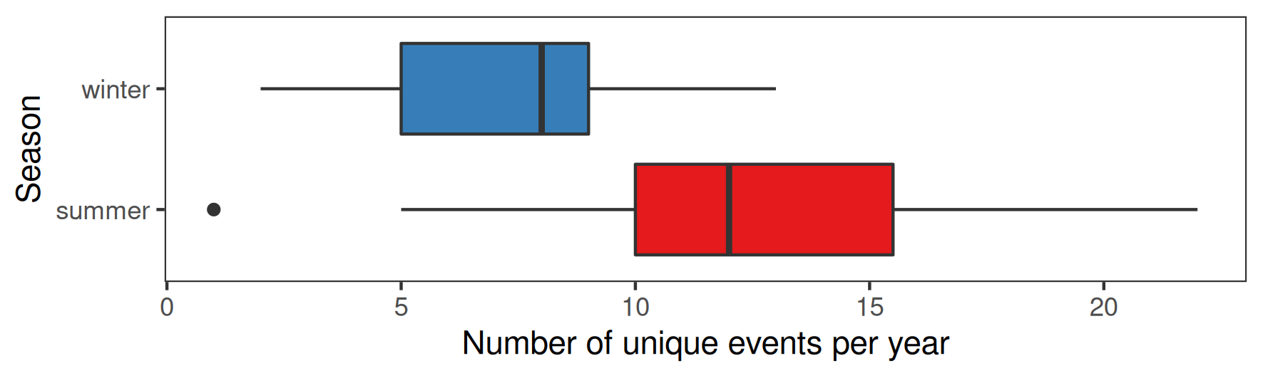
Figure 9: Boxplots showing the difference in unique events for the different seasons studied. Only the 24 hour data is shown.

Figure 9 shows how many unique events that resulted in block maxima were seen from the daily $i^{\mathrm{(sum,win)}}_{24,l}$ series. Overall, the number of unique events in summer is larger than in winter.

Appendix C OFS correction for Bayesian Inference using composite likelihood

A comparison between the uncorrected raw samples from the MCMC sampling using Stan with the pairwise likelihood of Eq. (16) and the corresponding samples corrected using the Open-Faced Sandwich (OFS) correction from (Shaby, 2014) is shown in Fig. 10. It can be seen that the uncorrected samples grossly underestimate the uncertainty shown by the 95% credibility intervals. On the other hand, the OFS corrected samples keep the same median but “stretch” the resulting uncertainty so that the desired 95% coverage of the intervals is achieved.

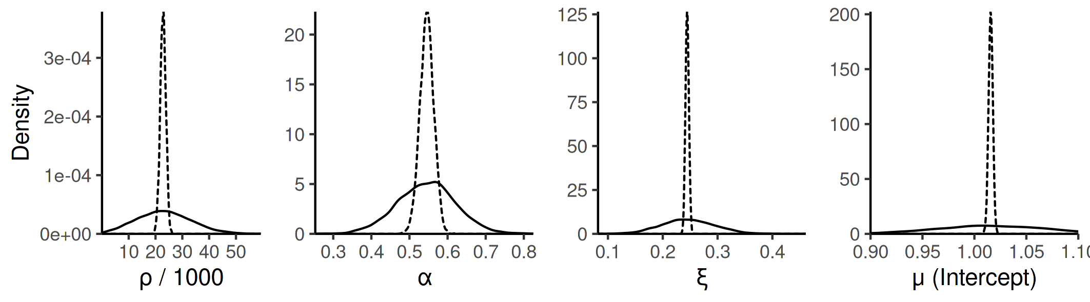
Figure 10: Density plots for the raw MCMC samples (dashed line) and the resulting OFS corrected samples (continuous lines) for 4 selected parameters from the daily summer results.

Appendix D Analysis of asymptotic dependence using extremal coefficient

Figure 11 shows the distribution of bootstraped samples for $\hat{\theta}_{\mathrm{NP}}(s_{j},s_{j^{\prime}})$, where the estimation method is the same as the one used for Fig. 4. The bootstraped samples provide an estimate of the uncertainty that allows us to judge the asymptotic dependence conditions present in the data.

The figure shows that for the daily series, both seasons show a value of the extremal coefficient below 1.75 for $h\leq 150$ km, suggesting that the data is asymptotically dependent at least for this distance. After 150 km, the coefficient goes close to 2, but not immediately. On the other hand, the situation is different between summer and winter for the hourly frequency. Here, the uncertainty is much larger, which could be a reflection of the smaller number of years. Furthermore, while the winter series behaves similar to the daily winter series having reasonably strong dependence for distances up to 150 km, the hourly summer series tends very quickly to lower dependence levels. This again suggests that the events in summer are typically smaller in size that those in winter. Asymptotical dependence can be reasonably suggested for the hourly winter data, but for hourly summer, one could argue this is true only for relatively short distances. However, the uncertainty is rather large, wit a lot of values still falling under the strong dependence case. Therefore, we make the assumption for asymptotical dependence for all four series.

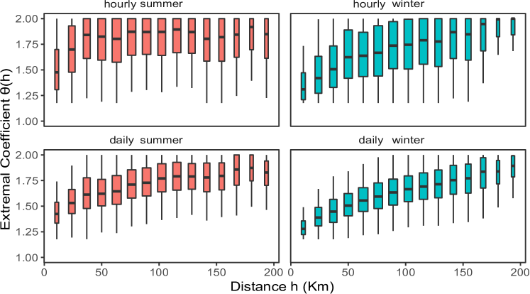
Figure 11: Boxplots showing the distribution of bootstraped samples (N=500) of the non-parametrical estimate of the extremal coefficient $\hat{\theta}_{\mathrm{NP}}(s_{j},s_{j^{\prime}})$. The width of the boxplots is proportional to the amount of data.

Appendix E Model diagnostic and posterior predictive checks for reference stations

We obtained Quantile-Quantile plots and Posterior predictive checks to assure that our model adequately represents the observed data. Some of these are shown in Fig. 12. The included plots come from the hourly summer data.

The QQ plots for the different stations provide evidence that the GEV is mostly appropriate for modeling the marginal distributions, with some minor exceptions. Similarly, the posterior predictive checks allow us to see how well the posterior distributions for the DM and BR models would be at capturing the original data. In this case, both models’ original data seems well-captured.

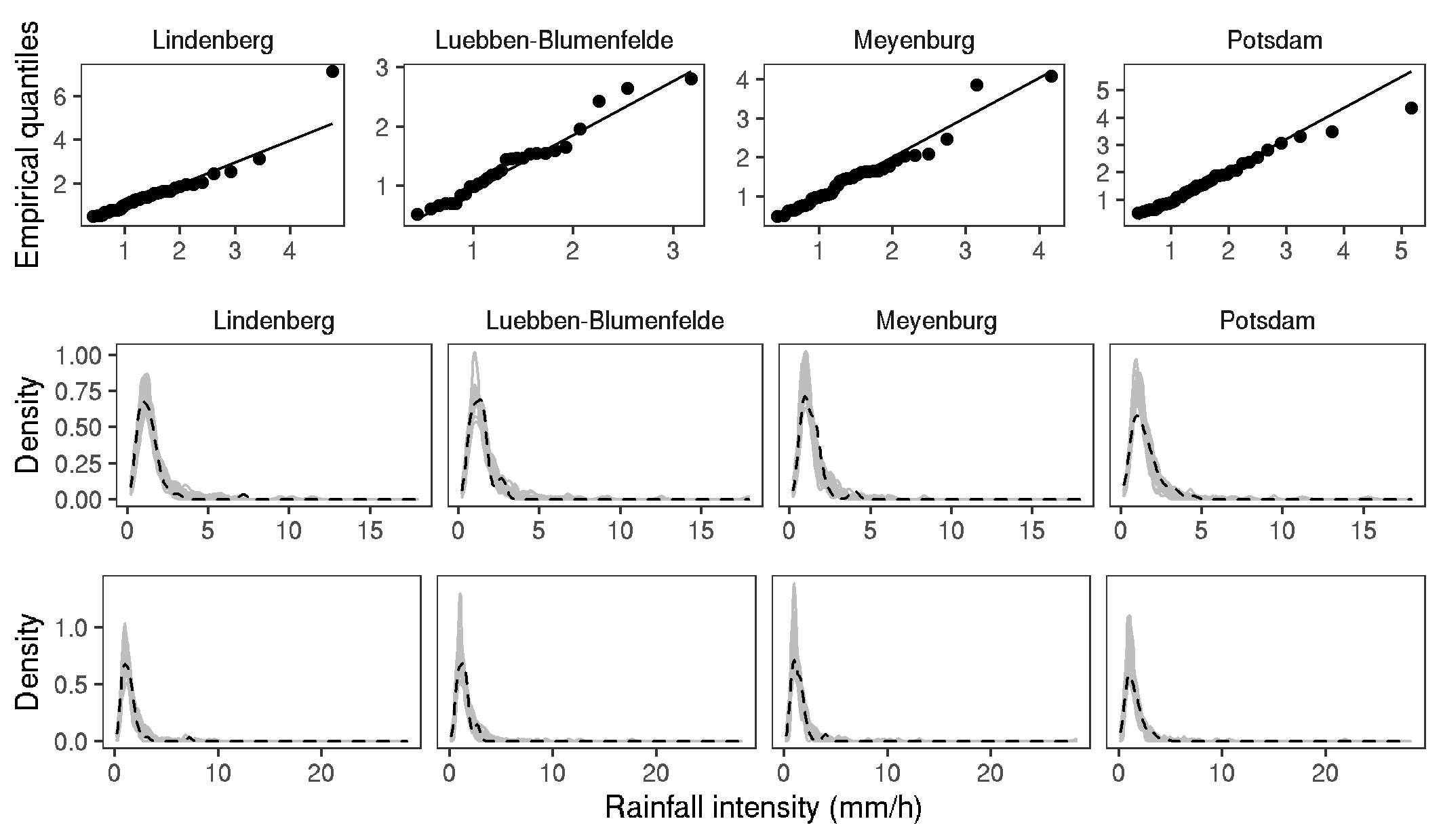
Figure 12: Top row: Q-Q plots for the four reference stations. Middle row: Posterior predictive check for the DM model. Bottom row: Posterior predictive check for the BR model. For the middle and bottom row, the dashed line shows the observed density, and the grey lines show 100 samples from 20 GEV distributions with parameters sampled from the respective posterior distributions.

References

- Durrans [2010] S. Rocky Durrans. Intensity-duration-frequency curves. In Rainfall: State of the Science, pages 159–169. American Geophysical Union (AGU), 2010. ISBN 9781118670231. doi:https://doi.org/10.1029/2009GM000919.
- Coles [2001] Stuart Coles. An Introduction to Statistical Modeling of Extreme Values. Springer, 2001. ISBN 978-1-84996-874-4. doi:10.1198/tech.2002.s73.
- Serinaldi [2015] Francesco Serinaldi. Dismissing return periods! Stoch. Environ. Res. Risk Assess., 29(4):1179–1189, 2015. ISSN 14363259. doi:10.1007/s00477-014-0916-1.
- Rootzén and Katz [2013] Holger Rootzén and Richard W. Katz. Design Life Level: Quantifying risk in a changing climate. Water Resour. Res., 49(9):5964–5972, 2013. ISSN 19447973. doi:10.1002/wrcr.20425.
- Davison and Gholamrezaee [2012] A. C. Davison and M. M. Gholamrezaee. Geostatistics of extremes. Proc. R. Soc. A Math. Phys. Eng. Sci., 468(2138):581–608, 2012. doi:10.1098/rspa.2011.0412.
- Tobler [1970] Waldo R Tobler. A computer movie simulating urban growth in the detroit region. Economic geography, 46(sup1):234–240, 1970.
- Davison and Huser [2015] A. C. Davison and Raphaël Huser. Statistics of Extremes. Ssrn, 2015. doi:10.1146/annurev-statistics-010814-020133.
- Padoan et al. [2010] S. A. Padoan, M. Ribatet, and S. A. Sisson. Likelihood-based inference for max-stable processes. J. Am. Stat. Assoc., 105(489):263–277, 2010. doi:10.1198/jasa.2009.tm08577.
- Le et al. [2018] Phuong Dong Le, Michael Leonard, and Seth Westra. Modeling Spatial Dependence of Rainfall Extremes Across Multiple Durations. Water Resour. Res., 54(3):2233–2248, mar 2018. doi:10.1002/2017WR022231.
- Davison et al. [2012] A. C. Davison, S. A. Padoan, and M. Ribatet. Statistical Modeling of Spatial Extremes. Stat. Sci., 27(2):161–186, 2012. doi:10.1214/11-STS376.
- Buhl and Klüppelberg [2016] Sven Buhl and Claudia Klüppelberg. Anisotropic Brown-Resnick space-time processes: estimation and model assessment. Extremes, 2016. doi:10.1007/s10687-016-0257-1.
- Berg and Haerter [2013] P. Berg and J. O. Haerter. Unexpected increase in precipitation intensity with temperature - A result of mixing of precipitation types? Atmos. Res., 119:56–61, 2013. ISSN 01698095. doi:10.1016/j.atmosres.2011.05.012.
- Walther and Bennartz [2006] Andi Walther and Ralf Bennartz. Radar-based precipitation type analysis in the Baltic area. Tellus, Ser. A Dyn. Meteorol. Oceanogr., 58(3):331–343, 2006. doi:10.1111/j.1600-0870.2006.00183.x.
- Orlanski [1975] Isidoro Orlanski. A rational subdivision of scales for atmospheric processes. Bulletin of the American Meteorological Society, 56:527–530, 1975.
- Bohnenstengel et al. [2011] Sylvia I. Bohnenstengel, K. H. Schlünzen, and F. Beyrich. Representativity of in situ precipitation measurements - A case study for the LITFASS area in North-Eastern Germany. J. Hydrol., 400(3-4):387–395, 2011. doi:10.1016/j.jhydrol.2011.01.052.
- Fischer et al. [2017] M Fischer, H.W. Rust, and U Ulbrich. A spatial and seasonal climatology of extreme precipitation return-levels: A case study. Spat. Stat., 2017.
- Ulrich et al. [2020a] Jana Ulrich, Oscar E Jurado, and Henning W Rust. Estimating IDF curves consistently over durations with spatial covariates. Water (Switzerland), 2020a.
- Boessenkool [2021] Berry Boessenkool. rdwd: Select and Download Climate Data from ’DWD’ (German Weather Service), 2021. URL https://CRAN.R-project.org/package=rdwd. R package version 1.5.0.
- Koutsoyiannis et al. [1998] D. Koutsoyiannis, D. Kozonis, and A. Manetas. A mathematical framework for studying rainfall intensity-duration-frequency relationships. J. Hydrol., 206:118–135, 1998.
- Ulrich et al. [2020b] Jana Ulrich, Oscar E. Jurado, Madlen Peter, Marc Scheibel, and Henning W. Rust. Estimating idf curves consistently over durations with spatial covariates. Water, 12(11:3119), 2020b. ISSN 2073-4441. doi:10.3390/w12113119.
- Ribatet et al. [2016] Mathieu Ribatet, Clément Dombry, and Marco Oesting. Spatial extremes and max-stable processes. In Dipak K Dey and Jun Yan, editors, Extreme value modeling and risk analysis: methods and applications. CRC Press, 2016.
- Marcon et al. [2017] G. Marcon, S. A. Padoan, P. Naveau, P. Muliere, and J. Segers. Multivariate nonparametric estimation of the Pickands dependence function using Bernstein polynomials. J. Stat. Plan. Inference, 2017. ISSN 03783758. doi:10.1016/j.jspi.2016.10.004.
- Vettori et al. [2018] Sabrina Vettori, Raphaël Huser, and Marc G. Genton. A comparison of dependence function estimators in multivariate extremes. Stat. Comput., 28(3):525–538, 2018. doi:10.1007/s11222-017-9745-7.
- Beranger et al. [2021] Boris Beranger, Simone Padoan, and Giulia Marcon. ExtremalDep: Extremal Dependence Models, 2021. URL https://CRAN.R-project.org/package=ExtremalDep. R package version 0.0.3-4.
- Cooley et al. [2012] D. Cooley, Jessi Cisewski, Robert J. Erhardt, Soyoung Jeon, Elizabeth Mannshardt, Bernard Oguna Omolo, and Ying Sun. A survey of spatial extremes: Measuring spatial dependence and modeling spatial effects. 10(1):135–165, 2012.
- Umlauf and Kneib [2018] Nikolaus Umlauf and Thomas Kneib. A primer on Bayesian distributional regression. Stat. Modelling, 18(3-4):219–247, 2018. ISSN 14770342. doi:10.1177/1471082X18759140.
- Vehtari et al. [2017] Aki Vehtari, Andrew Gelman, and Jonah Gabry. Practical Bayesian model evaluation using leave-one-out cross-validation and WAIC. Stat. Comput., 27(5):1413–1432, 2017. doi:10.1007/s11222-016-9696-4.
- Ribatet [2013] Mathieu Ribatet. Spatial extremes: Max-stable processes at work. J. la Société Française Stat. Rev. Stat. appliquée, 154(2):156–177, 2013.
- Kabluchko et al. [2009] Zakhar Kabluchko, Martin Schlather, and Laurens de Haan. Stationary max-stable fields associated to negative definite functions. Ann. Probab., 37(5):2042–2065, 2009. doi:10.1214/09-AOP455.
- Stephenson [2016] Alec Stephenson. Bayesian inference for extreme value modelling. In Dipak K Dey and Jun Yan, editors, Extreme value modeling and risk analysis: methods and applications. CRC Press, 2016.
- Dyrrdal et al. [2015] Anita Verpe Dyrrdal, Alex Lenkoski, Thordis L Thorarinsdottir, and Frode Stordal. Bayesian hierarchical modeling of extreme hourly precipitation in norway. Environmetrics, 26(2):89–106, 2015.
- Fukutome et al. [2018] S Fukutome, A Schindler, and A Capobianco. Meteoswiss extreme value analyses: User manual and documentation. 3rd edition. Technical report, MeteoSwiss, 2018.
- Kruschke [2014] John Kruschke. Doing bayesian data analysis: A tutorial with r, jags, and stan. 2014.
- Zheng et al. [2015] Feifei Zheng, Emeric Thibaud, Michael Leonard, and Seth Westra. Assessing the performance of the independence method in modeling spatial extreme rainfall. Water Resour. Res., 51(9):7744–7758, sep 2015. doi:10.1002/2015WR016893.
- Stephenson et al. [2016] Alec G. Stephenson, Eric A. Lehmann, and Aloke Phatak. A max-stable process model for rainfall extremes at different accumulation durations. Weather Clim. Extrem., 13:44–53, 2016. doi:10.1016/j.wace.2016.07.002.
- Stan Development Team [2022] Stan Development Team. Stan modeling language users guide and reference manual, version 2.29.0, 2022. URL http://mc-stan.org/.
- Ribatet et al. [2012] M. Ribatet, D. Cooley, and A. C. Davison. Bayesian Inference from composite likelihoods, with an application to spatial extremes. 22(2):813–845, 2012. doi:10.5705/ss.2009.248.
- Chan and So [2017] Raymond K.S. Chan and Mike K.P. So. On the performance of the Bayesian composite likelihood estimation of max-stable processes. J. Stat. Comput. Simul., 87(15):2869–2881, 2017. doi:10.1080/00949655.2017.1342824.
- Shaby [2014] Benjamin A. Shaby. The Open-Faced Sandwich Adjustment for MCMC Using Estimating Functions. J. Comput. Graph. Stat., 23(3):853–876, 2014. doi:10.1080/10618600.2013.842174.
- Bentzien and Friederichs [2014] Sabrina Bentzien and Petra Friederichs. Decomposition and graphical portrayal of the quantile score. Q. J. R. Meteorol. Soc., 140(683):1924–1934, 2014. doi:10.1002/qj.2284.
- Wilks [2011] Daniel S Wilks. Statistical methods in the atmospheric sciences, volume 100. Academic press, 2011.
- Lengfeld et al. [2019] Katharina Lengfeld, Tanja Winterrath, Thomas Junghänel, Mario Hafer, and Andreas Becker. Characteristic spatial extent of hourly and daily precipitation events in Germany derived from 16 years of radar data. Meteorol. Zeitschrift, 28(5):363–378, 2019. doi:10.1127/metz/2019/0964.
- Dombry et al. [2017] Clément Dombry, Sebastian Engelke, and Marco Oesting. Bayesian inference for multivariate extreme value distributions. Electron. J. Stat., 11(2):4813–4844, 2017. doi:10.1214/17-EJS1367.
- Ganguli and Coulibaly [2017] Poulomi Ganguli and Paulin Coulibaly. Does nonstationarity in rainfall require nonstationary intensity-duration-frequency curves? Hydrol. Earth Syst. Sci., 21(12):6461–6483, 2017. doi:10.5194/hess-21-6461-2017.
- Lengfeld et al. [2021] Katharina Lengfeld, Ewelina Walawender, Tanja Winterrath, and Andreas Becker. Catrare: A catalogue of radar-based heavy rainfall events in germany derived from 20 years of data. Meteorologische Zeitschrift, 30(6):469–487, 12 2021. doi:10.1127/metz/2021/1088. URL http://dx.doi.org/10.1127/metz/2021/1088.
- Wadsworth and Tawn [2019] Jennifer L Wadsworth and Jonathan Tawn. Higher-dimensional spatial extremes via single-site conditioning. arXiv preprint arXiv:1912.06560, 2019.
- Richards et al. [2021] Jordan Richards, Jonathan A. Tawn, and Simon Brown. Modelling extremes of spatial aggregates of precipitation using conditional methods, 2021. URL https://arxiv.org/abs/2102.10906.