Weakly bounded cohomology classes and a counterexample to a conjecture of Gromov

Abstract

We exhibit a finitely presented group whose second cohomology contains a weakly bounded, but not bounded, class. As an application, we disprove a long-standing conjecture of Gromov about bounded primitives of differential forms on universal covers of closed manifolds.

1 Introduction

Let $G$ be a group. We consider the cohomology of $G$ with coefficients in $A=\mathbb{Z}$ or $A=\mathbb{R}$. In particular, to compute $H^{*}(G;A)$ we take the bar resolution

where $C^{k}(G;A)$ denotes, for every $k\geq 0$, the group of arbitrary set maps from $G^{k}$ to $A$, and the coboundary maps are defined by the formula

$$(\delta\alpha)(g_{1},\dots,g_{k+1})\ =\ \alpha(g_{2},\dots,g_{k+1})+\sum_{i=1}^{k}(-1)^{i}\alpha(\dots,g_{i}g_{i+1},\dots)+(-1)^{k+1}\alpha(g_{1},\dots,g_{k}).$$

A cohomology class in $H^{k}(G;A)$ is bounded if it has a representative $\alpha:G^{k}\to A$ which is bounded, i.e. whose image is a bounded subset of $A$. A related notion is the following: a $k$-cochain $\alpha$ is weakly bounded if $\alpha(G,g_{2},\dots,g_{k})$ is a bounded subset of $A$ for every $g_{2},\dots,g_{k}\in G$. An element of $H^{k}(G;A)$ is weakly bounded if it is represented by a weakly bounded cocycle.

Of course, bounded cohomology classes are also weakly bounded, and in degrees $0$ and $1$ the two notions coincide (already at the cochain level). Neumann and Reeves, motivated by applications in the study of the coarse geometry of central extensions (see below for a brief description of this connection), asked in [NR96, NR97] whether a weakly bounded $2$-class on a finitely generated group is always bounded. Essentially the same question was considered by Whyte in [Why10, Remark 2.16].

Intimately related questions were posed by Wienhard and Blank, respectively in [Wie12, Question 8] and [Bla15, Question 6.3.10]. They asked under what conditions on $G$ a certain sequence of natural maps involving the bounded cohomology, the ordinary cohomology and the $\ell^{\infty}$-cohomology of $G$ (in some degree $k$) is exact; as shown in [FS20, Proposition 11], this is equivalent to asking under what conditions on $G$ weakly bounded classes in $H^{k}(G;A)$ are bounded. We refer to Section 2 for the definitions of bounded and $\ell^{\infty}$-cohomology and the precise reformulation of the question, which also comes in handy in later sections.

The main result of our paper is the following:

Theorem 1.1.

There exists a finitely presented group $G$ with a cohomology class in $H^{2}(G;\mathbb{Z})$ which is weakly bounded but not bounded.

This improves a recent result by Frigerio and Sisto, who had provided in [FS20, Corollary 10] a finitely generated, but not finitely presented, group with the same property. As a consequence of this improvement, we are able to disprove a related conjecture of Gromov, as we discuss below. It may be interesting to note that we can also obtain a group as in Theorem 1.1 which is non-elementary relatively hyperbolic (see Corollary 1.5).

Our construction is unrelated to the finitely generated example by Frigerio and Sisto. In fact, the property of not being finitely presentable plays a fundamental role in their construction, making it unlikely to manufacture a finitely presented example by a simple adaptation of their method.

It is appropriate to point out that, for a quite large and diverse family of groups $G$, weakly bounded cohomology classes in $H^{2}(G;\mathbb{Z})$ are bounded. As proved in [FS20], this family is closed under direct and free products (and also some amalgamated products), and includes amenable groups, relatively hyperbolic groups with respect to a finite family of amenable subgroups, right-angled Artin groups and fundamental groups of compact orientable $3$-manifolds.

In degrees $k\geq 3$ the situation is different, and it is quite easy to construct finitely presented groups $G$ with weakly bounded but not bounded cohomology classes in $H^{k}(G;\mathbb{Z})$. An example is given by $G=\mathbb{Z}^{k-2}\times\pi_{1}(\Sigma_{2})$, where $\Sigma_{2}$ is a closed orientable surface of genus $2$ (see [FS20, Corollary 3.3]).

Our example has the following presentation:

$$G=\langle a_{1},t_{1},a_{2},t_{2},b\ |\ [t_{1},a_{1}]=[t_{2},a_{2}]=b,[t_{1},b]=[t_{2},b]=1\rangle,$$ (1)

where $[x,y]=xyx^{-1}y^{-1}$ denotes the commutator of two elements. In Proposition 1.2 we highlight some additional properties of $G$; in particular, it is not only finitely presented, but also of type F.

Proposition 1.2.

The group $G$ defined by (1) is CAT(0) and of type F. More precisely, it admits a finite $2$-dimensional simplicial locally CAT(0) model, obtained by gluing a finite number of regular Euclidean triangles.

We now discuss some corollaries of Theorem 1.1.

Quasi-isometrically trivial central extensions

Let $G$ be a finitely generated group, and let

be a central extension of $G$ by $\mathbb{Z}$. Associated to such an extension there is an element of $H^{2}(G;\mathbb{Z})$, called the Euler class of the extension. The Euler class vanishes if and only if the extension is trivial, i.e. there is a commutative diagram of the form

where $h$ is a group isomorphism. The extension is said to be quasi-isometrically trivial if there is a diagram as above, with the following differences: $h$ is only required to be a quasi-isometry and the squares have to commute only up to a bounded error. Gersten proved in [Ger92, §3] that if the Euler class of the extension is bounded, then the extension is quasi-isometrically trivial. Then, Neumann and Reeves observed in [NR96] that the extension is quasi-isometrically trivial if and only if the Euler class is weakly bounded. A proof of this fact is provided in [FS20]. Thus, we get the following corollary of Theorem 1.1:

Corollary 1.3.

There is a quasi-isometrically trivial central extension of a finitely presented group $G$ by $\mathbb{Z}$ whose Euler class is not bounded.

This improves [FS20, Theorem 2], where the same phenomenon is exhibited by a finitely generated, but not finitely presented, group.

Gromov’s conjecture

Let $M$ be a closed connected Riemannian manifold, and let $[\omega]\in H_{\mathrm{dR}}^{2}(M)\cong H^{2}(M;\mathbb{R})$ be a cohomology class represented by a smooth differential $2$-form $\omega$. Gromov conjectured in [Gro93, page 93] that the following conditions are equivalent:

1. the pull-back $\widetilde{\omega}\in\Omega^{2}(\widetilde{M})$ on the universal cover of $M$ is the differential of a bounded form;

2. the class $[\omega]\in H_{\mathrm{dR}}^{2}(M)\cong H^{2}(M;\mathbb{R})$ is represented by a bounded singular cocycle.

It is easy to see that the first condition does not depend on the differential form $\omega$ representing the class. The implication (ii) $\Rightarrow$ (i) is true in any degree, and a self-contained proof is contained in [Sik01]. It is shown in [FS20, Corollary 20] that if a manifold $M$ satisfies Gromov’s statement then every weakly bounded class in $H^{2}(\pi_{1}(M);\mathbb{Z})$ is bounded. Therefore, a counterexample to the conjecture is given by any closed Riemannian manifold whose fundamental group is isomorphic to the group $G$ defined by the presentation (1). In Section 4, exploiting the fact that $G$ is of type $F$, we obtain an aspherical counterexample:

Corollary 1.4.

There exists a closed connected aspherical Riemannian manifold $M$ with a differential $2$-form $\omega\in\Omega^{2}(M)$ such that (i) holds but (ii) does not.

Using a result of Belegradek in [Bel06], we can also tweak the statement of Corollary 1.4 by requiring that the fundamental group of $M$ be non-elementary relatively hyperbolic. In particular, considering the group $\pi_{1}(M)$ we get the following strengthening of Theorem 1.1:

Corollary 1.5.

There exists a finitely presented group $G$ which is non-elementary relatively hyperbolic and has a cohomology class in $H^{2}(G;\mathbb{Z})$ which is weakly bounded but not bounded.

Structure of the paper

In Section 2 we recall the definitions of bounded and $\ell^{\infty}$-cohomology of groups and spaces, and reformulate the statement of Theorem 1.1 in terms of some natural maps between them. In Section 3, which is the heart of the paper, we prove Theorem 1.1. Finally, in Section 4 we prove Proposition 1.2 and Corollaries 1.4–1.5.

Acknowledgements

We thank Roberto Frigerio and Alessandro Sisto for helpful conversations about this problem and for the idea of considering amalgamated free products. We are grateful to Roberto Frigerio for his useful comments on preliminary drafts of the paper.

2 Bounded cohomology and $\bm{\ell^{\infty}}$-cohomology

The purpose of this section is to recall the definition of bounded and $\ell^{\infty}$-cohomology, and to formulate Theorem 1.1 using these objects.

The study of bounded cohomology is a very active research area which gained popularity after the fundamental paper of Gromov [Gro82]. Gersten introduced $\ell^{\infty}$-cohomology in [Ger92], and used it as a tool to obtain lower bounds for the Dehn function of finitely presented groups.

In the definitions below, we allow coefficients $A=\mathbb{Z}$ or $A=\mathbb{R}$. We also include the definition of bounded and $\ell^{\infty}$-cohomology of spaces, since in Section 3 we prefer to mostly work with spaces, instead of groups.

Bounded cohomology of groups

The bounded cohomology of $G$, denoted by $H_{b}^{*}(G;A)$, is defined as the cohomology of the subcomplex $C^{*}_{b}(G;A)\subseteq C^{*}(G;A)$ given by bounded cochains. The inclusion at the level of cochains induces the map $c^{*}:H_{b}^{*}(G;A)\to H^{*}(G;A)$ in cohomology.

$\ell^{\infty}$-cohomology of groups

The $\ell^{\infty}$-cohomology of $G$, denoted by $H_{\scriptscriptstyle{(\infty)}}^{*}(G;A)$, is defined as the cohomology of $G$ with coefficients in $\ell^{\infty}(G,A)$, the $A[G]$-module of bounded set functions from $G$ to $A$. The group $G$ acts on functions as usual: $(g\cdot f)(h)=f(g^{-1}h)$ for every $f\in\ell^{\infty}(G,A)$ and every $g,h\in G$. The inclusion of $A$ into $\ell^{\infty}(G,A)$ as the subgroup of constant functions induces the change of coefficients map $\iota^{*}:H^{*}(G;A)\to H_{\scriptscriptstyle{(\infty)}}^{*}(G;A)$ in cohomology.

Definitions for CW complexes

Let $X$ be a connected CW complex (this assumption is more restrictive than what is needed in the general theory, but suffices for our purposes). Denote by $G$ the fundamental group $\pi_{1}(X,*)$.

• The bounded cohomology of $X$, denoted by $H_{b}^{*}(X;A)$, is the cohomology of the complex of bounded singular cochains on $X$, where a cochain is bounded if the set of values it assigns to singular simplices is a bounded subset of $A$. The inclusion in the complex of singular cochains induces the map $c^{*}:H_{b}^{*}(X;A)\to H^{*}(X;A)$ in cohomology.

• The $\ell^{\infty}$-cohomology of $X$, denoted by $H_{\scriptscriptstyle{(\infty)}}^{*}(X;A)$, is defined as the singular equivariant cohomology of the universal cover of $X$ with coefficients in the $A[G]$-module $\ell^{\infty}(G,A)$. The inclusion of coefficients induces the map $\iota^{*}:H^{*}(X;A)\to H_{\scriptscriptstyle{(\infty)}}^{*}(X;A)$ in cohomology. Cellular cohomology can be used in place of singular cohomology, since the two are canonically isomorphic.

Remark.

On the other hand, the bounded cohomology of a CW complex cannot be computed using cellular cochains. For example, the bounded cohomology of the wedge of two circles is nontrivial in degree $2$, despite the absence of $2$-dimensional cells.

If $X$ is a $K(G,1)$ then there is a commutative diagram

where the vertical maps are canonical isomorphisms. The square on the right commutes because of the naturality of the change of coefficients $A\subseteq\ell^{\infty}(G,A)$, which gives the horizontal maps. For the definition of the leftmost vertical map and the commutativity of the square on the left see, e.g., [Iva17].

Reformulation of Theorem 1.1

The statement of Theorem 1.1 is equivalent to the following: there exists a finitely presented group $G$ such that the sequence of maps

(2)

is not exact at $H^{2}(G;\mathbb{Z})$.

The equivalence between the statement of Theorem 1.1 and the non-exactness of the sequence (2) descends immediately from the following facts:

• a class in $H^{k}(G;\mathbb{Z})$ is bounded if and only if it lies in the image of $c^{k}$;

• a class in $H^{k}(G;\mathbb{Z})$ is weakly bounded if and only if it lies in the kernel of $\iota^{k}$.

The first of the two facts follows directly from the definitions, while the second one is proved in [FS20, Proposition 11]. The two facts listed above also hold for real coefficients.

3 A weakly bounded but not bounded class

Consider the group $H=\langle a,b,t\ |\ tbt^{-1}=b,tat^{-1}=ba\rangle$. This is an HNN extension of the free group $F_{2}={\langle a,b\rangle}$. An equivalent way of writing the same presentation is $H=\langle a,b,t\ |\ [t,b]=1,[t,a]=b\rangle$.

Lemma 3.1.

For every $n\in\mathbb{N}$, the element $b^{n}\in H$ is a commutator.

Proof.

We show by induction on $n$ that $b^{n}=[t^{n},a]$. The base step is trivial. For the inductive step, assume that $b^{n}=[t^{n},a]$ and observe that

$$[t^{n+1},a]\ =\ t[t^{n},a]at^{-1}a^{-1}\ =\ tb^{n}at^{-1}a^{-1}\ =\ b^{n}tat^{-1}a^{-1}\ =\ b^{n+1}.$$

The conclusion follows. ∎

We consider the Cayley graph of $H$ with respect to the generating set $\{a,b,t\}$. This graph has a vertex for each element of $H$, and two vertices $h,h^{\prime}\in H$ are connected by an edge if and only if $h^{\prime}=hs$ for some $s\in\{a,b,t,a^{-1},b^{-1},t^{-1}\}$. We put on the Cayley graph the metric which assigns length $1$ to each edge, and we consider on $H$ the metric as a subspace of its Cayley graph.

We observe that every element of $H$ can be uniquely written as $t^{p}b^{q}w(a,b)$ where $p,q\in\mathbb{Z}$ and $w(a,b)$ is a reduced word in the letters $a,b$ (and in their inverses) such that $w(a,b)$ does not begin with $b$ or $b^{-1}$. Define the set map $\pi:H\rightarrow\mathbb{Z}$ given by $\pi(t^{p}b^{q}w(a,b))=q$. The map $\pi$ has the following two properties, which will be of fundamental importance in what follows.

Lemma 3.2.

The map $\pi:H\rightarrow\mathbb{Z}$ is $1$-Lipschitz.

Proof.

Consider an arbitrary element $h=t^{p}b^{q}w(a,b)$ where $w(a,b)$ does not begin with $b^{\pm 1}$. We proceed to show that $|\pi(h)-\pi(hs)|\leq 1$ for every $s\in\{a,b,t\}$. There is no need to consider multiplication by $s^{-1}$ separately, since $|\pi(h)-\pi(hs^{-1})|=|\pi(h^{\prime})-\pi(h^{\prime}s)|$ where $h^{\prime}=hs^{-1}$.

Write the word $t^{p}b^{q}w(a,b)a$ and reduce it: we have that at most one cancellation occurs, and, if it is the case, it involves the last two $a$ and $a^{-1}$ letters; in particular the exponent $q$ remains unchanged and thus $\pi(ha)=\pi(h)$.

Similarly, write the word $t^{p}b^{q}w(a,b)b$ and reduce it: again, at most one cancellation occurs, and, if it is the case, it involves the last two $b$ and $b^{-1}$ letters; if $w(a,b)$ is non-empty, the exponent $q$ remains unchanged; if $w(a,b)$ is empty, the exponent $q$ changes by exactly one. In any case we have $|\pi(hb)-\pi(h)|\leq 1$.

Finally, consider the element $t^{p}b^{q}w(a,b)t$ of $H$ and notice that it is equal to $t^{p+1}b^{q}w(b^{-1}a,b)$. The word $w(b^{-1}a,b)$ is obtained from $w(a,b)$ by substituting each occurrence of $a$ with $b^{-1}a$, and each occurrence of $a^{-1}$ with $a^{-1}b$. After performing this substitutions letter by letter, we obtain a possibly unreduced word which we can then reduce to $w^{\prime}(a,b)$. We observe that, during the reduction process, no $a$ or $a^{-1}$ letter gets canceled. If $w(a,b)$ begins with $a$, then $w^{\prime}(a,b)$ begins with $b^{-1}a$ and thus $\pi(ht)=q-1$; if $w(a,b)$ begins with $a^{-1}$, then $w^{\prime}(a,b)$ begins with $a^{-1}$ too and thus $\pi(ht)=q$; if $w(a,b)$ is empty, then $\pi(ht)=q$. In any case we have $|\pi(ht)-\pi(h)|\leq 1$. ∎

Lemma 3.3.

For every element $u\in H$, the restriction $\pi:u{\langle b\rangle}\rightarrow\mathbb{Z}$ to the coset $u{\langle b\rangle}$ is of one of the following forms:

1. it is a translation, i.e. $\pi(ub^{n})=c+n$ for some integer $c$;

2. it is constant on $u{\langle b\rangle}$, i.e. $\pi(ub^{n})=c$ for some integer $c$.

Moreover, the coset ${\langle b\rangle}$ falls into case (i).

Proof.

Let $u=t^{p}b^{q}w(a,b)$ so that $w(a,b)$ is reduced and does not begin with $b$ or $b^{-1}$. If $w(a,b)$ is non-empty, then $\pi(ub^{n})=q$ regardless of $n$, and thus we fall into case (ii). If $w(a,b)$ is empty, then $\pi(ub^{n})=n+q$ and thus we fall into case (i). Notice that with $u=1$ we fall into case (i). ∎

The map $\pi$ can be thought as a “retraction” from the group $H$ to ${\langle b\rangle}\cong\mathbb{Z}$. Similarly, we can retract $H$ on a generic coset $u{\langle b\rangle}$: for $u\in H$, define the map $\pi_{u}:H\rightarrow\mathbb{Z}$ given by $\pi_{u}(h)=\pi(u^{-1}h)$. From Lemma 3.2 and Lemma 3.3, it immediately follows that $\pi_{u}:H\rightarrow\mathbb{Z}$ is $1$-Lipschitz and that, for each $u^{\prime}\in H$, the restriction $\pi_{u}:u^{\prime}{\langle b\rangle}\rightarrow\mathbb{Z}$ of $\pi_{u}$ to the coset $u^{\prime}{\langle b\rangle}$ falls in one of cases (i) or (ii) of Lemma 3.3.

Lemma 3.4.

For two elements $u,u^{\prime}\in H$, the following are equivalent:

1. the restriction $\pi_{u}:u^{\prime}{\langle b\rangle}\rightarrow\mathbb{Z}$ falls into case (i) of Lemma 3.3;

2. the restriction $\pi_{u^{\prime}}:u{\langle b\rangle}\rightarrow\mathbb{Z}$ falls into case (i) of Lemma 3.3.

In this case we say that the cosets $u{\langle b\rangle}$ and $u^{\prime}{\langle b\rangle}$ are parallel.

Proof.

Each of the conditions holds if and only if $u^{\prime}=ut^{p}b^{q}$ for some $p,q\in\mathbb{Z}$. ∎

We are now ready to provide an example of a group together with a cohomology class which is weakly bounded but not bounded. As we will see, the class belongs to the cohomology of the group $G=H*_{\langle b\rangle}H$, given by the amalgamated free product of two copies of $H$, where we identify the two copies of the subgroup ${\langle b\rangle}$.

Remark.

In what follows, we will only make use of the conclusions of Lemmas 3.1–3.4. We can completely forget who $H$ is.

Let $Y$ be a CW complex consisting of one $0$-cell, three $1$-cells, oriented and labeled with $a,b,t$, two $2$-cells glued along the paths $tbt^{-1}b^{-1}$ and $tat^{-1}a^{-1}b^{-1}$, and cells in higher dimension in such a way that all the homotopy groups $\pi_{k}(Y,*)$ for $k\geq 2$ are trivial. From the construction, it is obvious that $Y$ is a $K(H,1)$.

We denote by $\widetilde{Y}$ the universal cover of $Y$. Each edge in the $1$-skeleton of $\widetilde{Y}$ inherits a label and an orientation (based on which edge of $Y$ it is mapped to by the covering map). Observe that the $1$-skeleton of $\widetilde{Y}$ is exactly the Cayley graph of $H$ with respect to the generating set $a,b,t$. If we fix a basepoint in the $0$-skeleton of $\widetilde{Y}$, this allows us to identify the $0$-cells of $\widetilde{Y}$ with the elements of $H$: the basepoint corresponds to the identity element of $H$, and crossing a $1$-cell corresponds to right multiplication by the label of the edge or its inverse, according to the orientation of the $1$-cell.

Consider the subspace of the $1$-skeleton of $\widetilde{Y}$ given by the union of all the closed edges labeled $b$: each connected component of such subspace is called a $\bm{b}$-line, and corresponds to a coset $u{\langle b\rangle}$ for some $u\in H$. We say that two $b$-lines are parallel if the two corresponding cosets are parallel (this does not depend on the choice of the basepoint).

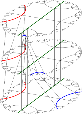
Figure 1: A portion of the $1$-skeleton of $\widetilde{Y}$, which coincides with the Cayley graph of $H$; the labeling has been omitted. The horizontal leaves are copies of the Cayley graph of $F_{2}={\langle a,b\rangle}$, and are joined by $1$-cells labeled with $t$ and oriented upward. For simplicity, only some of these $1$-cells are drawn. In bold we can see some $b$-lines, parallel $b$-lines having the same color.

Consider now the group $G=H*_{\langle b\rangle}H$. Let $S^{1}=\{z\in\mathbb{C}\colon\,|z|=1\}$ be the unit circle, and consider on $S^{1}\times[0,1]$ a structure of CW complex with two $0$-cells $(1,0),(1,1)$, three $1$-cells $S^{1}\times\{0\},S^{1}\times\{1\},\{1\}\times[0,1]$ and a single $2$-cell. Let $Y\cup_{b}Y$ be the CW complex obtained by taking two copies $Y_{0},Y_{1}$ of $Y$ and a copy of $S^{1}\times[0,1]$, and by gluing $S^{1}\times\{0\}$ to $Y_{0}$ along the $1$-cell labeled $b$, and by gluing $S^{1}\times\{1\}$ to $Y_{1}$ along the $1$-cell labeled $b$. We can take the gluing maps to be cellular, so that $X=Y\cup_{b}Y$ is a CW complex (see Figure 2); we observe that $\pi_{1}(X)\cong G$ and that $X$ is a $K(G,1)$.

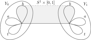
Figure 2: The space $X$ consists of two copies $Y_{0},Y_{1}$ of $Y$, together with a cylinder $S^{1}\times[0,1]$. For simplicity, in the figure we only drew the $1$-skeleton of $Y_{0}$ and $Y_{1}$. The boundary component $S^{1}\times\{0\}$ (resp. $S^{1}\times\{1\}$) of the cylinder is glued onto the $1$-cell labeled $b$ in $Y_{0}$ (resp. $Y_{1}$).

We denote by $\widetilde{X}$ the universal cover of $X$; it consists of infinitely many disjoint copies of $\widetilde{Y}$ and strips of the form $\mathbb{R}\times[0,1]$ covering the cylinder. Each side of each strip $\mathbb{R}\times[0,1]$ is glued along some $b$-line contained in some copy of $\widetilde{Y}$, and each $b$-line has exactly one side of one strip glued onto it (see Figure 3). The copies of $\widetilde{Y}$ and the strips $\mathbb{R}\times[0,1]$ are glued in a “tree-like” fashion, as we now explain. Take the space $\widetilde{X}$ and collapse each copy of $\widetilde{Y}$ to a single point; also, collapse each strip $\mathbb{R}\times[0,1]$ to a segment by taking the projection on the second component; we obtain a quotient space $T$ which is a graph, with one vertex corresponding to each copy of $\widetilde{Y}$, and one edge corresponding to each strip $\mathbb{R}\times[0,1]$. The graph $T$ is a tree, since $\widetilde{X}$ is simply connected, and each vertex has valence $\aleph_{0}$. It is the Bass-Serre tree corresponding to the amalgamated product $H*_{\langle b\rangle}H$. Call $\tau:\widetilde{X}\rightarrow T$ the quotient map.

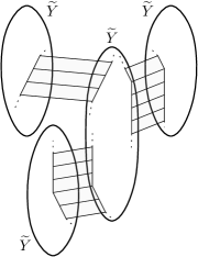
Figure 3: A portion of the space $\widetilde{X}$, with some disjoint copies of $\widetilde{Y}$ and some strips isomorphic to $\mathbb{R}\times[0,1]$. Each side of each strip is glued onto a $b$-line in some copy of $\widetilde{Y}$.

Let $\overline{e}$ be the unique $2$-cell of $X$ coming from the unique $2$-cell of $S^{1}\times[0,1]$. We consider the cellular cohomology of the complex $X$; let $\alpha\in C^{2}_{\mathrm{CW}}(X;\mathbb{Z})$ be the map given by $\alpha(\overline{e})=1$ and $\alpha(e)=0$ for every other $2$-cell $e\not=\overline{e}$. We observe that, since no $3$-cell of $X$ is attached on $\overline{e}$, we have $\delta\alpha=0$ and thus $\alpha$ defines a cohomology class $[\alpha]\in H^{2}_{\mathrm{CW}}(X;\mathbb{Z})$. Via the canonical isomorphism between $H^{2}_{\mathrm{CW}}(X;\mathbb{Z})$ and $H^{2}(G;\mathbb{Z})$, we obtain a class in $H^{2}(G;\mathbb{Z})$; our goal is to show that this class is weakly bounded but not bounded.

From integral to real coefficients.

We define $\alpha_{\mathbb{R}}\in C_{\mathrm{CW}}^{2}(X;\mathbb{R})$ to be the cochain corresponding to $\alpha$ under the change of coefficients map induced by the inclusion $\mathbb{Z}\subseteq\mathbb{R}$. By [FS20, Lemma 2.8], passing to real coefficients does not interfere with (weakly) boundedness of cohomology classes. Therefore, to establish Theorem 1.1, it is enough to show that $[\alpha_{\mathbb{R}}]\in H^{2}_{\mathrm{CW}}(X;\mathbb{R})\cong H^{2}(G;\mathbb{R})$ is weakly bounded but not bounded. Hereafter, when we say that a class in cellular cohomology is (weakly) bounded, we mean that the mentioned property is enjoyed by the corresponding class in the cohomology of $G$ via the canonical isomorphism.

Proposition 3.5.

The cohomology class $[\alpha_{\mathbb{R}}]\in H^{2}_{\mathrm{CW}}(X;\mathbb{R})\cong H^{2}(G;\mathbb{R})$ is not bounded.

Proof.

Let $S_{2}$ denote the closed orientable surface of genus $2$, and let $S_{1,1}$ denote the compact orientable surface of genus $1$ and with one boundary component (i.e. the torus with a hole). Fix $n\in\mathbb{N}$: since by Lemma 3.1 the element $b^{n}$ is a commutator, there is a continuous map $\varphi:S_{1,1}\rightarrow Y$ that restricts to a degree $n$ map between $\partial S_{1,1}$ and the $1$-cell labeled by $b$.

We now take the two copies $Y_{0},Y_{1}$ of $Y$, and we consider two copies of the surface $S_{1,1}$ along with the two copies $\varphi_{0}:S_{1,1}\rightarrow Y_{0}$ and $\varphi_{1}:S_{1,1}\rightarrow Y_{1}$ of the map $\varphi$. We look at $Y_{0},Y_{1}$ as subspaces of $X=Y\cup_{b}Y$, and we apply homotopies to the maps $\varphi_{0},\varphi_{1}$, pushing $\varphi_{0}(\partial S_{1,1})$ and $\varphi_{1}(\partial S_{1,1})$ along the cylinder $S^{1}\times[0,1]$, until the two maps eventually meet at the meridian $S^{1}\times\{1/2\}$. At this point we can glue together the two domains of the maps $\varphi_{0},\varphi_{1}$ in order to obtain a map $\psi:S_{2}\rightarrow Y$ which covers the cell $\overline{e}$ with degree $n$.

Suppose that $[\alpha_{\mathbb{R}}]\in H^{2}_{\mathrm{CW}}(X;\mathbb{R})\cong H^{2}(G;\mathbb{R})$ is bounded. This implies that there is a bounded singular cocycle $\alpha_{s}\in C^{2}(X;\mathbb{R})$ whose class $[\alpha_{s}]\in H^{2}(X;\mathbb{R})$ corresponds to $[\alpha_{\mathbb{R}}]$ under the canonical isomorphism between singular and cellular cohomology. Let $L\in\mathbb{R}$ be such that $|\alpha_{s}(\sigma)|\leq L$ for every singular simplex $\sigma$ in $X$, and notice that also the norm of the pull-back $\psi^{*}\alpha_{s}\in C^{2}(S_{2};\mathbb{R})$ is bounded by the same constant $L$. Let $[S_{2}]\in H_{2}(S_{2},\mathbb{R})$ be the fundamental class. Since $\psi$ covers the cell $\overline{e}$ with degree $n$, we have that

$$n\ =\ \langle[\alpha_{s}],\ \psi_{*}[S_{2}]\rangle\ =\ \langle\psi^{*}[\alpha_{s}],\ [S_{2}]\rangle\ \leq\ L\|S_{2}\|$$

where $\|S_{2}\|$ denotes the simplicial volume of $S_{2}$, which is equal to $4$. Thus we obtain that $L\geq n/4$; this cannot hold for all $n\in\mathbb{N}$, contradiction. ∎

Remark.

In the proof of Proposition 3.5 we use the fact that $b^{n}$ is a commutator for every $n\in\mathbb{N}$, but this hypothesis can be relaxed; in fact, the same result can be obtained using only the weaker hypothesis that the stable commutator length of $b$ is zero; the proof is essentially the same.

It remains to prove that the class $[\alpha_{\mathbb{R}}]\in H^{2}_{\mathrm{CW}}(X;\mathbb{R})\cong H^{2}(G;\mathbb{R})$ is weakly bounded. In this part of the proof we use Lemma 3.2 and Lemma 3.3 to obtain a kind of isoperimetric inequality for $1$-cycles in $\widetilde{X}$, with respect to appropriate notions of perimeter and area. First, we consider combinatorial circuits in $\widetilde{X}$, introduce a purely combinatorial definition for the area of a circuit, and prove a linear isoperimetric inequality for it (Proposition 3.11). Then, we deduce an analogous inequality for cellular $1$-cycles, which allows us to conclude that $[\alpha_{\mathbb{R}}]$ is weakly bounded.

We begin by defining the combinatorial objects we are interested in. A path in a CW complex is a finite non-empty list of $0$-cells $p=(p_{0},p_{1},\dots,p_{k})$ such that, for every $i\in\{1,\dots,k\}$, $p_{i-1}$ and $p_{i}$ are the endpoints of a $1$-cell. We denote by $\mathrm{Len}(p)$ its length, which in the example above is equal to $k$. We call $p$ a circuit if its first and last $0$-cells coincide.

Recall that $X=Y\cup_{b}Y$ is obtained by gluing a cylinder $S^{1}\times[0,1]$ and two copies $Y_{0},Y_{1}$ of $Y$. We call $l=\{1\}\times[0,1]\subseteq S^{1}\times[0,1]$ the only $1$-cell not contained in $Y_{0}$ or $Y_{1}$. We also fix on $l$ the usual orientation of $[0,1]$; intuitively, the positive orientation corresponds to going away from $Y_{0}$ towards $Y_{1}$.

Recall that $\widetilde{X}$ consists of infinitely many disjoint copies of $\widetilde{Y}$ and strips of the form $\mathbb{R}\times[0,1]$ covering the cylinder $S^{1}\times[0,1]$. Consider the $1$-cells $l_{n}=\{n\}\times[0,1]\subseteq\mathbb{R}\times[0,1]$ given by the liftings of $l$. Given a strip $s$ in $\widetilde{X}$, we can choose an isomorphism of $s$ with $\mathbb{R}\times[0,1]$ preserving the covering map to $S^{1}\times[0,1]$.

Definition 3.6.

Let $p=(p_{0},p_{1},\dots,p_{k})$ be a circuit in $\widetilde{X}$. Let $s$ be a strip in $\widetilde{X}$ and choose an isomorphism $s\cong\mathbb{R}\times[0,1]$. We define $\mathrm{Area}_{s}(p)\in\mathbb{Z}$ by summing the following contributions, for $i\in\{1,\dots,k\}$:

1. if $\partial l_{n}=p_{i}-p_{i-1}$ for some $n\in\mathbb{Z}$, we sum $n$;

2. if $\partial l_{n}=-p_{i}+p_{i-1}$ for some $n\in\mathbb{Z}$, we sum $-n$;

3. otherwise, the index $i$ does not contribute to the sum.

Lemma 3.7.

The value of $\mathrm{Area}_{s}(p)$ does not depend on the chosen isomorphism $s\cong\mathbb{R}\times[0,1]$.

Proof.

Suppose we are given two isomorphisms $\eta_{1},\eta_{2}:s\rightarrow\mathbb{R}\times[0,1]$ that both commute with the covering space projections $s\rightarrow S^{1}\times[0,1]$ and $\mathbb{R}\times[0,1]\rightarrow S^{1}\times[0,1]$. Then it is easy to see that $\eta_{1},\eta_{2}$ only differ by an integer translation along the $\mathbb{R}$ component, i.e. $\eta_{2}=\eta_{1}+(r,0)$ for some $r\in\mathbb{Z}$.

Recall that there is a projection $\tau:\widetilde{X}\rightarrow T$ of $\widetilde{X}$ onto a tree, and that $s$ is sent to an edge of $T$. Removing the interior of $\tau(s)$ divides $T$ into two connected components $T_{0},T_{1}$. Whenever $p$ goes from $T_{0}$ to $T_{1}$ (i.e. for each $i$ such that $\tau(p_{i})\in T_{1}$ and $\tau(p_{i-1})\in T_{0}$) we have a summand in the definition of $\mathrm{Area}_{s}(p)$ according to case 1 of Definition 3.6; whenever $p$ goes from $T_{1}$ to $T_{0}$ we have a summand in the definition of $\mathrm{Area}_{s}(p)$ according to case 2 of Definition 3.6. The number of times $p$ goes from $T_{0}$ to $T_{1}$ must be the same as the number of times $p$ goes from $T_{1}$ to $T_{0}$: this means that in the sum defining $\mathrm{Area}_{s}(p)$ the cases 1 and 2 occur the same number of times.

If we compute $\mathrm{Area}_{s}(p)$ using the identification $\eta_{2}$ instead of $\eta_{1}$, each summand coming from case 1 increases by $r$, and each summand coming from case 2 decreases by $r$. Since cases 1 and 2 occur the same number of times, the sum $\mathrm{Area}_{s}(p)$ remains unchanged, as desired. ∎

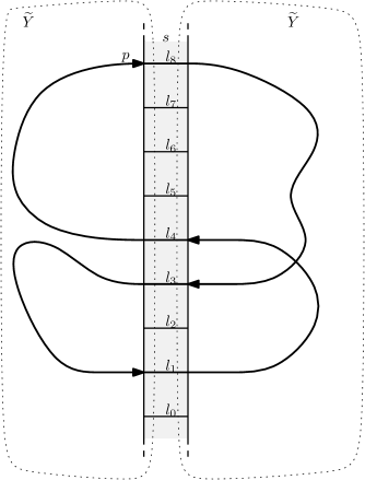
Figure 4: An example of a circuit $p$ that crosses a strip $s$ four times. Edges $l_{1},l_{8}$ are crossed with positive orientation, while edges $l_{3},l_{4}$ are crossed with negative orientation; thus in this case $\mathrm{Area}_{s}(p)=1+8-3-4=2$. Informally, $\mathrm{Area}_{s}(p)$ is equal to the number of squares of $s$ “enclosed” by $p$, counted with sign.

Definition 3.8.

We define $\mathrm{Area}(p)=\sum_{s}\mathrm{Area}_{s}(p)$ where $s$ varies among all the strips in $\widetilde{X}$.

Lemma 3.9.

Let $p=(p_{0},\dots,p_{k})$ be a circuit in $\widetilde{X}$. Let $V$ be a copy of $\widetilde{Y}$ in $\widetilde{X}$, and let $\lambda$ be a $b$-line in $V$. Denote by $S_{\lambda}$ the set of the strips $s$ such that one side of $s$ is glued on a $b$-line in $V$ which is parallel to $\lambda$. Let $\mathrm{Len}_{V}(p)$ be the number of indices $i\in\{1,\dots,k\}$ such that $p_{i-1},p_{i}$ both belong to $V$. Then we have

$$\left\lvert\sum\limits_{s\in S_{\lambda}}\mathrm{Area}_{s}(p)\right\rvert\ \leq\ \mathrm{Len}_{V}(p).$$

Proof.

Recall that $X=Y_{0}\cup_{b}Y_{1}$ and without loss of generality assume that $V$ projects to $Y_{0}$. Also assume that $p_{0}=p_{k}$ belongs to $V$. Choose a basepoint in $V$ belonging to the $b$-line $\lambda$; this gives an identification between the vertices of $V$ and the elements of $H$, and in particular the map $\pi:H\rightarrow\mathbb{Z}$ induces a map from the set of the vertices of $V$ to $\mathbb{Z}$.

Let $p_{x_{0}},...,p_{y_{0}},p_{x_{1}},...,p_{y_{1}},...,p_{x_{r}},...,p_{y_{r}}$ be the set of vertices of $p$ that belong to $V$, with $0=x_{0}\leq y_{0}\leq x_{1}\leq y_{1}\leq...\leq x_{r}\leq y_{r}=k$ and with $x_{i}-y_{i-1}\geq 2$ for $i=1,...,r$. We now look at the sequence of integers $\pi(p_{x_{0}}),\pi(p_{y_{0}}),\pi(p_{x_{1}}),\pi(p_{y_{1}}),...,\pi(p_{x_{r}}),\pi(p_{y_{r}})$.

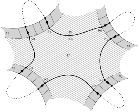
Figure 5: An example of a circuit $p$ entering $V$ four times.

By Lemma 3.2 the map $\pi$ is $1$-Lipschitz, and thus we have $|\pi(p_{y_{i}})-\pi(p_{x_{i}})|\leq|y_{i}-x_{i}|$ for $i=0,...,r$.

For $i=1,...,r$, we have that $p_{y_{i-1}},p_{y_{i-1}+1}$ belong to a same strip $s_{i}$ with one side glued on $V$, and similarly $p_{x_{i}-1},p_{x_{i}}$ belong to a same strip $s^{\prime}_{i}$ with one side glued on $V$. Using the projection map $\tau:\widetilde{X}\rightarrow T$ and the fact that $T$ is a tree, it is easy to see that $s_{i}=s^{\prime}_{i}$. We also observe that these are the only cases where the path $p$ crosses a strip with a side glued onto $V$.

If $s_{i}$ is glued onto $V$ along a $b$-line which is not parallel to $\lambda$, then $\pi(p_{x_{i}})-\pi(p_{y_{i-1}})=0$ since $p_{x_{i}},p_{y_{i-1}}$ belong to a same $b$-line which is sent to a constant value. If $s$ is glued onto $V$ along a $b$-line $\lambda^{\prime}$ parallel to $\lambda$, then there are two edges $l_{n},l_{m}$ of $s_{i}$ with $\partial l_{n}=p_{y_{i-1}+1}-p_{y_{i-1}}$ and $\partial l_{m}=p_{x_{i}-1}-p_{x_{i}}$. Since the map $\pi$ is a translation on the vertices of $\lambda^{\prime}$, it easily follows that $\pi(p_{x_{i}})-\pi(p_{y_{i-1}})=m-n$, and notice that $m$ and $-n$ are two summands that appear in the definition of $\mathrm{Area}_{s}(p)$. For each strip $s$ glued to $V$ onto a $b$-line parallel to $\lambda$, each summand in the definition of $\mathrm{Area}_{s}(p)$ appears exactly once when $i$ ranges from $1$ to $r$; this implies that

$$\sum\limits_{s\in S_{\lambda}}\mathrm{Area}_{s}(p)\ =\ \sum\limits_{i=1}^{r}\pi(p_{x_{i}})-\pi(p_{y_{i-1}}).$$

It follows that

$$\left\lvert\sum\limits_{s\in S_{\lambda}}\mathrm{Area}_{s}(p)\right\rvert\ =\ \left\lvert\sum\limits_{i=1}^{r}\pi(p_{x_{i}})-\pi(p_{y_{i-1}})\right\rvert\ =\ \left\lvert-\sum\limits_{i=0}^{r}\pi(p_{y_{i}})-\pi(p_{x_{i}})\right\rvert$$

$$\leq\ \sum\limits_{i=0}^{r}|\pi(p_{y_{i}})-\pi(p_{x_{i}})|\ \leq\ \sum\limits_{i=0}^{r}|y_{i}-x_{i}|\ =\ \mathrm{Len}_{V}(p)$$

as desired. ∎

Recall that we have a quotient map $\tau:\widetilde{X}\rightarrow T$ that collapses each copy of $\widetilde{Y}$ to a point and each strip $\mathbb{R}\times[0,1]$ to a segment, and that the quotient space $T$ is a tree.

We introduce a coloring, i.e. an equivalence relation, on the set of the edges of $T$. Suppose we have two strips $s_{1},s_{2}\cong\mathbb{R}\times[0,1]$; suppose that $s_{1}$ has one side glued onto a $b$-line $\lambda_{1}$ in a copy of $\widetilde{Y}$, and that $s_{2}$ has one side glued onto a $b$-line $\lambda_{2}$ in the same copy of $\widetilde{Y}$; suppose also that $\lambda_{1},\lambda_{2}$ are parallel in that copy of $\widetilde{Y}$. Then we define the two edges $\tau(s_{1}),\tau(s_{2})$ to be equivalent. On the set of edges of $T$, we take the equivalence relation generated by these equivalences: this gives a coloring of the edges of $T$.

Lemma 3.10.

There is a coloring of a subset of the vertices of $T$ such that, for each edge $s$ of $T$, the edge $s$ has exactly one endpoint of its same color.

Proof.

Fix a vertex $v_{0}$ of $T$ and let $S(v_{0},n)$ be the set of vertices of $T$ which have distance exactly $n$ from $v_{0}$. We define by induction on $n$ a partial coloring on $S(v_{0},n)$.

For $S(v_{0},0)=\{v_{0}\}$ we just leave the vertex $v_{0}$ uncolored. Suppose we have defined the partial coloring on $S(v_{0},n)$. Take a vertex $v\in S(v_{0},n+1)$: then there is a unique edge $e$ connecting $v$ to a vertex $v^{\prime}\in S(v_{0},n)$. If $v^{\prime}$ has the same color as $e$, then we leave $v$ uncolored; otherwise, we give $v$ the same color as $e$.

Since $S(v_{0},n)$ for $n\in\mathbb{N}$ form a partition of the set of vertices of $T$, this defines a partial coloring on the set of vertices of $T$. For how the partial coloring is defined, it is immediate to see that it has the desired property. ∎

Now we have a coloring of the edges and of a subset of vertices of $T$ with the following properties: given two strips $s_{1},s_{2}$ with a side glued onto a same copy $V$ of $\widetilde{Y}$, we have that $\tau(s_{1}),\tau(s_{2})$ have the same color if and only if the two strips $s_{1},s_{2}$ are glued onto parallel $b$-lines in $V$; for each strip $s$ with the sides glued on two copies $V_{1},V_{2}$ of $\widetilde{Y}$, we have that exactly one of $\tau(V_{1}),\tau(V_{2})$ has the same color as $\tau(s)$. We now use this coloring to prove the following fundamental proposition.

Proposition 3.11.

Let $p=(p_{0},p_{1},\dots,p_{k})$ be a circuit in $\widetilde{X}$. Then $|\mathrm{Area}(p)|\leq\mathrm{Len}(p)$.

Proof.

Suppose $s$ is a strip of the form $\mathbb{R}\times[0,1]$ in $\widetilde{X}$. The edge $\tau(s)$ has a certain color, and exactly one of its endpoints has the same color: call $V(s)$ the $\tau$-preimage of that vertex; this means that $V(s)$ is a copy of $\widetilde{Y}$, and $\tau(V(s))$ is a vertex of $T$ with the same color as the edge $\tau(s)$.

Let now $V$ be a copy of $\widetilde{Y}$ in $\widetilde{X}$. Suppose there is a strip $s$ with $V(s)=V$: then for every strip $s^{\prime}$ we have that $V(s^{\prime})=V$ if and only if $s^{\prime}$ is glued on $V$ and $\tau(s^{\prime})$ has the same color as $\tau(s)$; notice that, by definition, $\tau(s^{\prime})$ has the same color as $\tau(s)$ if and only if they are glued onto two parallel $b$-lines in $V$. Thus we can apply Lemma 3.9 and we have that

$$\left\lvert\sum\limits_{\begin{subarray}{c}s\text{ with}\\ V(s)=V\end{subarray}}\mathrm{Area}_{s}(p)\right\rvert\ \leq\ \mathrm{Len}_{V}(p)$$

where the sum on the left is finite since $p$ can only touch a finite number of strips. It follows that

$$\left\lvert\mathrm{Area}(p)\right\rvert\ =\ \left\lvert\sum\limits_{\begin{subarray}{c}s\text{ strip}\end{subarray}}\mathrm{Area}_{s}(p)\right\rvert\ \leq\ \sum\limits_{\begin{subarray}{c}V\text{ copy}\\ \text{of }\widetilde{Y}\end{subarray}}\left\lvert\sum\limits_{\begin{subarray}{c}s\text{ with}\\ V(s)=V\end{subarray}}\mathrm{Area}_{s}(p)\right\rvert\ \leq\ \sum\limits_{\begin{subarray}{c}V\text{ copy}\\ \text{of }\widetilde{Y}\end{subarray}}\mathrm{Len}_{V}(p)\ \leq\ \mathrm{Len}(p)$$

where the sums have only a finite number of non-zero summands, since the circuit $p$ touches a finite number of copies of $\widetilde{Y}$ and of strips. The conclusion follows. ∎

If $p$ is a path in $\widetilde{X}$, it uniquely determines a sequence of $1$-cells; we denote by $\overline{p}\in C_{1}^{\mathrm{CW}}(\widetilde{X};\mathbb{R})$ the cellular $1$-chain given by the sum of these cells, with a sign depending on the direction in which the $1$-cell is crossed. If $p$ is a circuit, then $\overline{p}$ is a $1$-cycle.

We denote by $\widetilde{\alpha}_{\mathbb{R}}\in C_{\mathrm{CW}}^{2}(\widetilde{X};\mathbb{R})$ the pull-back of $\alpha_{\mathbb{R}}\in C_{\mathrm{CW}}^{2}(X;\mathbb{R})$ via the covering map.

Lemma 3.12.

Let $p=(p_{0},p_{1},\dots,p_{k})$ be a circuit in $\widetilde{X}$. Denote by $\overline{p}\in C_{1}^{\mathrm{CW}}(\widetilde{X};\mathbb{R})$ the cellular $1$-cycle induced by $p$. Let $c\in C_{2}^{\mathrm{CW}}(\widetilde{X};\mathbb{R})$ be such that $\overline{p}=\partial c$. Then $\widetilde{\alpha}_{\mathbb{R}}(c)=\mathrm{Area}(p)$.

Proof.

Let $s\cong\mathbb{R}\times[0,1]$ be a strip in $\widetilde{X}$. As in Definition 3.6, we denote by $l_{n}$ the $1$-cell $\{n\}\times[0,1]\subseteq s$. Let $I^{+}\subseteq\{1,\dots,k\}$ be the subset of indices $i$ such that $p_{i}-p_{i-1}=\partial l_{n}$ for some $n\in\mathbb{Z}$, and set $f(i)=n$ for such indices. That is, $i\in I^{+}$ if the $i$-th step of $p$ crosses $s$ positively along the $1$-cell $l_{f(i)}$. Similarly, let $I^{-}\subseteq\{1,\dots,k\}$ be the subset of indices $i$ with $-p_{i}+p_{i-1}=\partial l_{n}$ for some $n\in\mathbb{Z}$, and set $f(i)=n$ for such indices. By definition, we have

$$\mathrm{Area}_{s}(p)\ =\ \sum_{i\in I^{+}}f(i)-\sum_{i\in I^{-}}f(i).$$

For every $n\in\mathbb{Z}$ we denote by $Q_{n}=[n,n+1]\times[0,1]\subseteq s$ the $2$-cell between $l_{n}$ and $l_{n+1}$. Consider the following $2$-chain:

$$c_{s}\ =\ \sum_{n\in\mathbb{Z}}\left(\#\{i\in I^{+}\colon\,f(i)\geq n+1\}-\#\{i\in I^{-}\colon\,f(i)\geq n+1\}\right)Q_{n}.$$

The sum has a finite number of non-zero terms, because if $n$ is small enough (say, $n<-M$ for a suitable integer $M$), then the two terms whose difference is the coefficient of $Q_{n}$ are the cardinalities of $I^{+}$ and $I^{-}$, which are equal (as we noticed in the proof of Lemma 3.7); on the other hand, if $n$ is large enough then both terms vanish. We now evaluate $\widetilde{\alpha}_{\mathbb{R}}$ at $c_{s}$:

$$\widetilde{\alpha}_{\mathbb{R}}(c_{s})\ =\ \sum_{n\in\mathbb{Z}}\left(\#\{i\in I^{+}\colon\,f(i)\geq n+1\}-\#\{i\in I^{-}\colon\,f(i)\geq n+1\}\right)$$

$$=\ \sum_{n\geq-M}\left(\#\{i\in I^{+}\colon\,f(i)\geq n+1\}-\#\{i\in I^{-}\colon\,f(i)\geq n+1\}\right)$$

$$=\ \sum_{i\in I^{+}}\#\{n\geq-M\colon\,f(i)\geq n+1\}-\sum_{i\in I^{-}}\#\{n\geq-M\colon\,f(i)\geq n+1\}$$

$$=\ \sum_{i\in I^{+}}(f(i)+M)-\sum_{i\in I^{-}}(f(i)+M)$$

$$=\ M(\#I^{+}-\#I^{-})+\sum_{i\in I^{+}}f(i)-\sum_{i\in I^{-}}f(i)$$

$$=\ \mathrm{Area}_{s}(p).$$

The $2$-chain $c_{s}$ also has the following important property: for every $n\in\mathbb{Z}$, the $1$-cell $l_{n}$ appears in $\partial c_{s}$ with coefficient $\#\{i\in I^{+}\colon\,f(i)=n\}-\#\{i\in I^{-}\colon\,f(i)=n\}$, which is equal to the coefficient of $l_{n}$ in $\overline{p}=\partial c$.

Let $c^{\prime}=\sum_{s}c_{s}$, with $s$ varying in the set of strips in $\widetilde{X}$. The sum is finite because $c_{s}=0$ unless the circuit $p$ crosses $s$ at some point, and $p$ crosses only finitely many strips. The $1$-cycle $\partial(c-c^{\prime})$ is supported in the (disconnected) subspace $\pi^{-1}(Y)\subseteq\widetilde{X}$ whose components are the various copies of $\widetilde{Y}$. Since every component of $\pi^{-1}(Y)$ is simply connected, there is a $2$-chain $c^{\prime\prime}$ with support in $\pi^{-1}(Y)$ such that $\partial c^{\prime\prime}=\partial(c-c^{\prime})$. This implies that $\widetilde{\alpha}_{\mathbb{R}}(c^{\prime\prime})=\widetilde{\alpha}_{\mathbb{R}}(c-c^{\prime})$, because $\widetilde{\alpha}_{\mathbb{R}}$ is exact. We now have

$$\widetilde{\alpha}_{\mathbb{R}}(c)\ =\ \widetilde{\alpha}_{\mathbb{R}}(c^{\prime\prime})+\widetilde{\alpha}_{\mathbb{R}}(c^{\prime})\ =\ 0+\sum_{s}\widetilde{\alpha}_{\mathbb{R}}(c_{s})\ =\ \sum_{s}\mathrm{Area}_{s}(p)\ =\ \mathrm{Area}(p),$$

which is the desired equality. ∎

Proposition 3.13.

The cohomology class $[\alpha_{\mathbb{R}}]\in H^{2}_{\mathrm{CW}}(X;\mathbb{R})\cong H^{2}(G;\mathbb{R})$ is weakly bounded.

Proof.

Recall from Section 2 that the class $[\alpha_{\mathbb{R}}]$ is weakly bounded if and only if its corresponding class in the singular cohomology $H^{2}(X;\mathbb{R})$ lies in the kernel of the change of coefficient map $\iota^{2}:H^{2}(X;\mathbb{R})\to H_{\scriptscriptstyle{(\infty)}}^{2}(X;\mathbb{R})=H^{2}(X;\ell^{\infty}(G,\mathbb{R}))$. Here, we prefer to work directly with cellular cochains, and show that $[\alpha_{\mathbb{R}}]$ lies in the kernel of $\iota_{\mathrm{CW}}:H_{\mathrm{CW}}^{2}(X;\mathbb{R})\to H_{\mathrm{CW}}^{2}(X;\ell^{\infty}(G;\mathbb{R}))$. To prove this claim, we use [Mil21, Theorem 5.1], that characterizes the kernel of $\iota_{\mathrm{CW}}$ in terms of a linear isoperimetric inequality: $\iota_{\mathrm{CW}}([\alpha_{\mathbb{R}}])=0$ if and only if there is a constant $L\in\mathbb{R}$ such that $|\widetilde{\alpha}_{\mathbb{R}}(c)|\leq L\|\partial c\|_{1}$ for every $c\in C_{2}^{\mathrm{CW}}(\widetilde{X};\mathbb{R})$. We proceed to show this inequality with $L=1$.

Let $c\in C_{2}^{\mathrm{CW}}(\widetilde{X};\mathbb{R})$. The boundary of $c$ is a cellular $1$-cycle, and we express it as

$$\partial c\ =\ \lambda_{1}\overline{p_{1}}+\lambda_{2}\overline{p_{2}}+\dots+\lambda_{k}\overline{p_{k}}$$

where each $\overline{p_{i}}$ is the $1$-cycle associated to a circuit $p_{i}$, the coefficients $\lambda_{i}$ are non-negative real numbers, and no cancellation occurs in the sum, i.e. $\|\partial c\|_{1}=\lambda_{1}\mathrm{Len}(p_{1})+\dots+\lambda_{k}\mathrm{Len}(p_{k})$. Every $1$-cycle can be expressed in this way, as it is easy to prove by induction on the number of summands appearing in the linear combination of $1$-cells defining the cycle.

For every $i\in\{1,\dots,k\}$ let $c_{i}\in C_{2}^{\mathrm{CW}}(\widetilde{X};\mathbb{R})$ be a $2$-chain such that $\partial c_{i}=\overline{p_{i}}$. It exists because $\widetilde{X}$ is simply connected. By linearity of the boundary operator, we have $\partial c=\partial(\lambda_{1}c_{1}+\dots+\lambda_{k}c_{k})$. This implies that $\widetilde{\alpha}_{\mathbb{R}}(c)=\widetilde{\alpha}_{\mathbb{R}}(\lambda_{1}c_{1}+\dots+\lambda_{k}c_{k})$, because $\widetilde{\alpha}_{\mathbb{R}}$ is an exact $2$-cocycle.

Applying in order the triangular inequality, Lemma 3.12 and Proposition 3.11 we obtain that

$$|\widetilde{\alpha}_{\mathbb{R}}(c)|\ =\ |\widetilde{\alpha}_{\mathbb{R}}(\lambda_{1}c_{1}+\dots+\lambda_{k}c_{k})|$$

$$\leq\ \lambda_{1}|\widetilde{\alpha}_{\mathbb{R}}(c_{1})|+\dots+\lambda_{k}|\widetilde{\alpha}_{\mathbb{R}}(c_{k})|$$

$$=\ \lambda_{1}|\mathrm{Area}(p_{1})|+\dots+\lambda_{k}|\mathrm{Area}(p_{k})|$$

$$\leq\ \lambda_{1}\mathrm{Len}(p_{1})+\dots+\lambda_{k}\mathrm{Len}(p_{k})$$

$$=\ \|\partial c\|_{1},$$

which is the inequality we wanted to prove. ∎

4 A 2-dimensional CAT(0) model

Let $G$ be the group constructed in Section 3. In this section we build a locally CAT(0) $2$-dimensional simplicial complex whose fundamental group is isomorphic to $G$, thus proving Proposition 1.2.

Recall that the group $G$ is defined as the amalgamated product $G=H*_{\langle b\rangle}H$, where

$$H=\langle a,b,t\ |\ tbt^{-1}=b,tat^{-1}=ba\rangle.$$ (3)

By introducing two auxiliary letters, we can equivalently write

$$H=\langle a,b,t,x,y\ |\ by=t,ax=y,yb=t,xa=t\rangle.$$ (4)

In fact, from the first two relations in (4) we get $y=b^{-1}t$ and $x=a^{-1}b^{-1}t$; by substituting these expressions in the last two relations we recover (equivalent forms of) the relations in (3).

Proof of Proposition 1.2.

We start by constructing a locally CAT(0) $2$-dimensional $K(H,1)$, that we call $Y$. Then, the desired $K(G,1)$ is obtained from two copies of $Y$ and a flat cylinder, by gluing the boundary components of the cylinder along closed geodesics representing the element $b\in H$ in the two copies of $Y$.

We build $Y$ as a CW complex with one $0$-cell, five $1$-cells and four triangular $2$-cells. We denote the $0$-cell by $v$, and label the five $1$-cells with the letters $a$,$b$,$t$,$x$ and $y$. The four $2$-cells are glued as shown in Figure 6. The fundamental group of $Y$ is isomorphic to $H$, since the four triangles in Figure 6 precisely encode the relations appearing in the presentation (4).

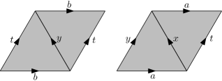
Figure 6: How to glue the $2$-cells of $Y$ to the $1$-skeleton.

We obtain a simplicial complex by subdividing every $2$-cell of $Y$ as shown in Figure 7. Then, we endow each $2$-simplex of the subdivision with the metric of a regular Euclidean triangle, and consider the resulting path metric on $Y$.

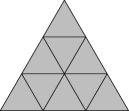
Figure 7: How to subdivide the $2$-cells of $Y$ to obtain a simplicial complex.

We now check that $Y$ is a locally CAT(0) metric space. By [BH99, Chapter II, Theorems 5.2 and 5.6], $Y$ is locally CAT(0) if and only if its vertex links don’t contain injective loops of length less than $2\pi$. For vertices distinct from $v$ (coming from the subdivision of a $1$-cell or $2$-cell), this conditions is very easily checked. We now consider the link of $v$.

The link of $v$ is a metric $1$-dimensional simplicial complex, whose $1$-simplices all have length $\pi/3$: they correspond to the angles of the triangles in Figure 6. This $1$-complex has ten vertices and twelve edges, and it is clear from Figure 8 that every injective loop in it has length at least $2\pi$. This implies that $Y$ is locally CAT(0). In particular, the universal cover of $Y$ is CAT(0), hence contractible, and $Y$ is a $K(H,1)$.

Figure 8: The link of $v$. It has ten vertices: every $1$-cell of $Y$ (before the subdivision) gives rise to two vertices, corresponding to its tail (_out) and its head (_in).

Consider now the $K(G,1)$ obtained by taking two disjoint copies of $Y$ and gluing isometrically the boundary components of a flat cylinder to the $1$-cells labeled with $b$, one in each copy of $Y$. We triangulate the cylinder as in Figure 9, with the lower and upper sides glued to the $1$-cell $b$ of the first and second copies of $Y$, respectively (recall that $b$ has been subdivided in three $1$-simplices).

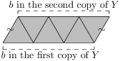
Figure 9: How to triangulate the cylinder.

The link of $v$ changes as follows: three more vertices and edges are added, forming a path from $b_{\mathrm{out}}$ to $b_{\mathrm{in}}$ of length $\pi/2$. This operation does not introduce any circuit of length less than $\pi$, so the resulting $K(G,1)$ is locally CAT(0), as desired. ∎

We now use the fact that $G$ has a finite simplicial model to construct an aspherical counterexample to Gromov’s conjecture, thus proving Corollary 1.4.

Proof of Corollary 1.4.

Let $N$ be a compact smooth manifold with boundary which is homotopy equivalent to the finite simplicial $K(G,1)$ constructed in the proof of Proposition 1.2. Such a manifold can be obtained by replacing $k$-dimensional simplices with $4$-dimensional $k$-handles. In particular, $N$ is aspherical and its fundamental group is isomorphic to $G$.

We apply the Davis’ reflection group trick described in [Dav08, §11.1] to $(N,\partial N)$, obtaining a closed smooth manifold $M$ together with continuous maps $\iota:N\to M$ and $r:M\to N$ whose composition $r\circ\iota:N\to N$ is the identity.

Let $[\alpha]\in H^{2}(G;\mathbb{Z})$ be the weakly bounded but not bounded class considered in Section 3. It is clear from the definitions that the pull-back of a (weakly) bounded cohomology class is (weakly) bounded. Therefore, $r^{*}([\alpha])\in H^{2}(\pi_{1}(M);\mathbb{Z})$ is weakly bounded. On the other hand it cannot be bounded, because $\iota^{*}r^{*}([\alpha])\in H^{2}(G;\mathbb{Z})$ is equal to $[\alpha]$, which is unbounded.

So $H^{2}(\pi_{1}(M);\mathbb{Z})$ contains a weakly bounded but not bounded class. By [FS20, Corollary 20] it follows that $M$ (endowed with an arbitrary Riemannian metric) has a $2$-form $\omega$ that satisfies the two conditions in the statement. ∎

Belegradek proved in [Bel06] that for any closed aspherical (smooth or PL) $n$-manifold $M$ there is a closed aspherical $(n+1)$-manifold $M^{\prime}$ in the same category such that $M^{\prime}$ retracts onto $M$ and $\pi_{1}(M^{\prime})$ is hyperbolic relative to $\pi_{1}(M)$. By applying this result to the manifold $M$ of Corollary 1.4, we obtain another aspherical counterexample to Gromov’s conjecture, with the additional property that its fundamental group is non-elementary relatively hyperbolic. This also proves Corollary 1.5.

References

- [Bel06] Igor Belegradek. Aspherical manifolds, relative hyperbolicity, simplicial volume and assembly maps. Algebr. Geom. Topol., 6:1341–1354, 2006. doi:10.2140/agt.2006.6.1341.
- [BH99] Martin R. Bridson and André Haefliger. Metric spaces of non-positive curvature, volume 319 of Grundlehren Math. Wiss. Springer-Verlag, Berlin, 1999. doi:10.1007/978-3-662-12494-9.
- [Bla15] Matthias Blank. Relative bounded cohomology for groupoids. PhD thesis, Regensburg University, 2015. Available at https://epub.uni-regensburg.de/31298/.
- [Dav08] Michael W. Davis. The geometry and topology of Coxeter groups, volume 32 of London Math. Soc. Monographs Ser. Princeton Univ. Press, Princeton, NJ, 2008. press.princeton:9780691131382.
- [FS20] Roberto Frigerio and Alessandro Sisto. Central extensions and bounded cohomology, 2020. arXiv:2003.01146.
- [Ger92] Stephen M. Gersten. Bounded cohomology and combings of groups, 1992. CiteSeerX:10.1.1.626.2986.
- [Gro82] Mikhael Gromov. Volume and bounded cohomology. Publ. Math. IHÉS, 56:5–99, 1982. numdam:PMIHES_1982__56__5_0.
- [Gro93] Mikhael Gromov. Volume 2: Asymptotic invariants of infinite groups. In Geometric Group Theory, volume 182 of Lond. Math. Soc. Lecture Note Ser., pages vii+295. Cambridge Univ. Press, Cambridge, 1993. doi:10.1017/CBO9780511629273.
- [Iva17] Nikolai V. Ivanov. Notes on the bounded cohomology theory, 2017. arXiv:1708.05150.
- [Mil21] Francesco Milizia. -cohomology: amenability, relative hyperbolicity, isoperimetric inequalities and undecidability, 2021. arXiv:2107.09089.
- [NR96] Walter D. Neumann and Lawrence Reeves. Regular cocycles and biautomatic structures. Internat. J. Algebra Comput., 6(3):313–324, 1996. doi:10.1142/S0218196796000167.
- [NR97] Walter D. Neumann and Lawrence Reeves. Central extensions of word hyperbolic groups. Ann. of Math. (2), 145(1):183–192, 1997. doi:10.2307/2951827.
- [Sik01] Jean-Claude Sikorav. Growth of a primitive of a differential form. Bull. Soc. Math. France, 129(2):159–168, 2001. doi:10.24033/bsmf.2390.
- [Why10] Kevin Whyte. Coarse bundles, 2010. arXiv:1006.3347.
- [Wie12] Anna Wienhard. Remarks on and around bounded differential forms. Pure Appl. Math. Q., 8(2):479–496, 2012. doi:10.4310/PAMQ.2012.V8.N2.A5.