Classical Limit of Higher-Spin String Amplitudes

Abstract

It has been shown that a special set of three-point amplitudes between two massive spinning states and a graviton reproduces the linearised stress-energy tensor for a Kerr black hole in the classical limit. In this work we revisit this result and compare it to the analysis of the amplitudes describing the interaction of leading Regge states of the open and closed superstring. We find an all-spin result for the classical limit of two massive spinning states interacting with a photon or graviton. This result differs from Kerr and instead matches the current four-vector and the stress-energy tensor generated by a classical string coupled to electromagnetism and gravity respectively. For the superstring amplitudes, contrary to the black-hole case, we find that the spin to infinity limit is necessary to reproduce the classical spin multipoles.

1 Introduction

Massive higher-spin scattering amplitudes have received a lot of attention in the past decade for their role in calculating classical gravity observables. Early work by ref. Vaidya:2014kza suggested that amplitudes between low-spin massive states and gravitons could be used to compute the lowest orders in the spin-multipole expansion of black hole observables, such as scattering angles and gravitational potentials. Later an all-order in spin result was obtained when a special set of arbitrary-spin three-point amplitudes in ref. Arkani-Hamed:2017jhn was used to calculate the linearised energy-momentum tensor of a Kerr black hole, and therefore extract the conservative dynamics of a binary system of spinning black holes at leading order in the post-Minkowskian (PM) expansion Vines:2017hyw ; Guevara:2017csg ; Guevara:2018wpp ; Chung:2018kqs ; Guevara:2019fsj ; Chung:2020rrz .

The double copy, Kawai:1985xq ; Bern:2008qj ; Bern:2010ue ; Bern:2019prr , and its extension to massive states, has proved to be a powerful tool when calculating the relevant gravitational amplitudes from their simpler Yang-Mills counterparts Johansson:2015oia ; Ochirov:2018uyq ; Johansson:2019dnu ; Chung:2019duq ; Bautista:2019evw ; Arkani-Hamed:2019ymq ; Edison:2020ehu ; Johnson:2020pny ; Momeni:2020hmc ; Momeni:2020vvr ; Haddad:2020tvs ; Emond:2020lwi ; Bjerrum-Bohr:2020syg ; Brandhuber:2021kpo . This field theoretic relation leaves an imprint in the classical theory in the form of the classical double copy, which was first introduced by ref. Monteiro:2014cda to relate the structure of Schwarzschild and Kerr black hole solutions to corresponding solutions in classical electrodynamics. Conversely, tools used to relate classical solutions, such as the Newman-Janis shift, have since been exported to the amplitudes framework providing simplifications in the treatment of spin Huang:2019cja ; Chung:2019yfs ; Guevara:2020xjx .

The classically relevant spin information can be extracted after the introduction of the Pauli-Lubanski spin operator, which connects quantum and classical spin Maybee:2019jus . Amplitudes can be expressed as polynomials in the expectation value of this operator, known as the spin multipole expansion Vaidya:2014kza , a process that has been facilitated by the use of the on-shell spinor-helicity variables introduced by ref. Arkani-Hamed:2017jhn and their extension, the on-shell HPET variables introduced in ref. Aoude:2020onz . The general approach to the classical limit of amplitudes can be summarised as taking the simultaneous $\hbar\to 0$ and quantum spin $s\to\infty$ limit while fixing $\hbar s\sim\mathcal{O}(1)$ as introduced in ref. Arkani-Hamed:2019ymq . Recently work in ref. Aoude:2021oqj provided an alternative formulation in terms of spin-coherent states. The three point amplitudes in ref. Arkani-Hamed:2017jhn exhibit special behaviour when expressed in terms of the spin variables described above. Any finite spin-$s$ amplitude reproduces the same spin multipole expansion that arises in the $s\to\infty$ limit, albeit only up to order $2s$ in the Pauli-Lubanski operator. This is referred to as spin universality Holstein:2008sw ; Holstein:2008sx and it makes it possible to extract classical observables from finite-spin amplitudes, up to a finite order in the spin multipole expansion. Moreover, the three-point Kerr amplitudes seem to have additional special features in the eikonal approximation including suppressed entanglement Aoude:2020mlg ; Chen:2021huj ; Haddad:2021znf .

Conservative observables for spinning black holes have since been studied in a variety of different frameworks, including higher-spin effective field theories and worldline quantum field theory Bern:2020buy ; Liu_2021 ; Jakobsen:2021lvp ; Jakobsen:2022fcj ; Riva:2022fru . The current state of the art for spinning observables at NLO (one loop) corresponds to quartic order in spin Guevara:2018wpp ; Chung:2018kqs ; Siemonsen:2019dsu ; Damgaard:2019lfh ; Bern:2020buy ; Kosmopoulos:2021zoq ; Chen:2021qkk ; Menezes:2022tcs and, at NNLO (two loop), quadratic order in spin Jakobsen:2022fcj ; FebresCordero:2022jts . Moreover, recent work extends beyond black holes by including tidal deformations Aoude:2020ygw ; Bern:2020uwk and going beyond conservative dynamics to the study of radiative observables, such as the waveform and the power emitted by a binary system Mogull:2020sak ; AccettulliHuber:2020dal ; Cristofoli:2021vyo ; Herrmann:2021lqe ; Jakobsen:2021lvp ; Mougiakakos:2021ckm ; Bautista:2021inx ; Alessio:2022kwv .

Despite this progress, a complete understanding of the effective theory that can match Kerr observables to all orders is still missing Bekaert:2022poo . In particular, the correct form of the gravitational Compton amplitude involving two massive spinning states and two gravitons, needed to extend the one-loop calculation to higher orders in spin, is still an open problem. A candidate Compton amplitude was computed in refs. Arkani-Hamed:2017jhn ; Johansson:2019dnu using factorisation and BCFW recursion relations Britto:2004ap ; Britto:2005fq , but the results developed spurious poles for any spin higher than two. Complementary approaches have emerged to tackle this problem. One seeks to resolve the ambiguity in the classical regime, extrapolating patterns that emerged in the one loop conservative observables for low spin to higher spins Aoude:2022trd ; Bern:2022kto ; Aoude:2022thd . For certain observables it was also shown that the details of the Compton amplitude can be ignored in the relevant regimes Alessio:2022kwv ; Chen:2022yxw . Alternatively, recent work by one of the authors, Chiodaroli:2021eug , sought to exploit the many constraints and consistency conditions that are present in higher-spin theory and derived the Kerr three-point amplitudes from first principles, up to spin-$5/2$ massive states, from high-energy unitarity considerations. The proposed spin-$5/2$ Compton amplitude, also appearing in ref. Falkowski:2020aso from a novel massive BCFW-type shift, has several nice properties as demonstrated in ref. Aoude:2022thd . However, it seems to be at odds with spin universality at quartic order in spin. At this point in time a first principles calculation of the Kerr Compton amplitude is still missing, however some progress has been made by mapping this problem to plane-wave scattering in a black-hole background as described by the Teukolsky equation Bautista:2021wfy .

This work also starts from the observation in ref. Chiodaroli:2021eug that the three-point Kerr amplitudes Arkani-Hamed:2017jhn are connected to highly constrained theories in the higher-spin literature. When looking for a well-behaved model of fundamental higher-spin particles that satisfies high-energy unitarity constraints, string theory is a natural place to consider. Various aspects of massive states in string theory have been studied for several decades, including work on properties of the spectrum and vertex operators KOH1987201 ; Berkovits:2002qx ; Hanany:2010da ; Bianchi:2010es ; Lust:2012zv ; Lee:2012fu ; Feng:2012bb ; Fu:2013xba , and amplitude computations that probe the interaction of massive and massless string states PhysRevD.83.046005 ; Feng:2010yx ; Schlotterer:2011zz ; Feng:2011qc ; Boels:2012if ; Tsulaia:2012rb ; Feng:2012qia ; Boels:2014dka ; Minahan:2014usa ; Hansen:2015pqa ; Chakrabarti:2018bah ; Lee:2019ufv ; Gross:2021gsj ; Jusinskas:2021bdj ; Guillen:2021mwp . In particular, the interaction of massive string states with gravity was the subject of several studies Giannakis:1998wi ; Buchbinder:1999be ; Buchbinder:1999ar ; Buchbinder:2000ta . Massive higher-spin particles in flat space are subject to no-go theorems and high-energy pathologies (see for example refs. PhysRev.186.1337 ; PhysRev.188.2218 ), hence studying massive string states offered valuable insight on how such issues can be circumvented Taronna:2010qq ; Joung:2012rv ; Taronna:2012gb ; Rahman:2015pzl ; Marotta:2021oiw . Exploring the high energy regime, where the higher-spin tower becomes most relevant, also leads to interesting observations that hint to a spontaneous-symmetry-breaking-like mechanism responsible for the particles’ mass Gross:1988ue ; Lee:1994fy ; Chan:2003ee ; Chan:2004tb ; Chan:2005ne ; Chan:2005zp ; Chan:2006qf ; Polyakov:2009pk ; Polyakov:2010qs ; Fotopoulos:2010ay ; Bianchi:2011se ; Lee:2019lvp ; Gross:2021gsj . An interesting example can be found in ref. Sagnotti:2010at , where the three-point amplitudes for massive states of the bosonic string are computed and uplifted to off-shell vertices to highlight their high-energy properties. Similarly ref. Schlotterer:2010kk provided general-spin amplitudes for leading Regge states of the open and closed superstring.

In this work, we study the leading Regge superstring amplitudes, in particular the three-point amplitudes between two massive spinning states and a photon/gluon or graviton, and apply the same classical limit technology that was introduced for the Kerr case. The resulting amplitudes, expanded in spin multipoles, are shown to agree with Kerr at the first mass level (quantum spin $s=4$, in the closed string case). However, for higher spin numbers, the results deviate from Kerr and, in the infinite-spin limit, they match the electromagnetic current and stress-energy tensor of known classical string solutions Ademollo:1974te ; Lust1989 ; zwiebach_2004 , manifesting a novel classical double copy relation between the two. The purpose of this work is twofold. First and foremost, it provides an application of the classical limit to a different set of amplitudes, highlighting important elements that are easily overlooked when studying the Kerr case. For instance, whereas the three-point Kerr amplitudes obey spin universality, the string amplitudes do not, such that the spin multipoles associated to the classical solutions can be reproduced only after taking the infinite-spin limit. Furthermore, this work paves the way to future investigations of the classical limit of string amplitudes. This includes exploring other string theories, such as bosonic and heterotic strings, as well as going beyond the leading Regge trajectory, including treatment of subleading trajectories as well as string coherent states Bianchi:2019ywd , in the hope that there exists a set of string amplitudes that generate the correct classical amplitudes for Kerr black holes.

The structure of this paper is as follows. In section 2 we define spin vector variables and review their application to classical limits of amplitudes, with emphasis on the Kerr black-hole case. In section 3 we apply the same technology to the string amplitudes between two leading Regge trajectory states and a photon or graviton, highlighting some conceptual differences to the black-hole case and computing the all-spin classical limit. This is shown to match some standard classical string solutions in section 4. We conclude in section 5 discussing our results and outlining some interesting future directions. In the appendix, we provide more detail on the classical string solutions we studied.

2 Spin Variables and Classical Limits

In this section we will review the formalism for the classical limit of three-point spinning amplitudes in the spirit of ref. Arkani-Hamed:2019ymq , presenting it in a form that is best suited to this work. We will start by introducing the spin variables that make the spin dependence in the amplitudes explicit.

2.1 Spin vector variables

Let us consider a spin-$s$ free particle in a quantum field theory, with momentum $p_{1}$ and mass $m$, satisfying the on-shell condition $p_{1}^{2}=m^{2}$. This can arise as an asymptotic state in a scattering amplitude and, as we will explain in more detail, it will be identified with a black hole or another classical object upon taking the classical limit. Its intrinsic spin is described by the expectation value of the Pauli-Lubanski operator

$$S^{\mu}_{(s)}=\frac{1}{2m}\epsilon^{\mu\nu\rho\sigma}p_{1\nu}M_{(s)\rho\sigma},$$ (1)

where the subscript $(s)$ indicates inserting the spin-$s$ representation of the Lorentz generators,

$${(M_{(s)\mu\nu})^{\alpha(s)}}_{\beta(s)}=\begin{cases}2is\,{\delta^{(\alpha_{1}}}_{[\mu}\eta_{\nu](\beta_{1}}\delta^{\alpha_{2}}_{\beta_{2}}\dots\delta^{\alpha_{s})}_{\beta_{s})}&\textrm{ for integer spin,}\vspace{3mm}\\ is\,{(\sigma_{\mu\nu})_{(\alpha_{1}}}^{(\beta_{1}}\delta^{\alpha_{2}}_{\beta_{2}}\dots\delta^{\alpha_{2s})}_{\beta_{2s})}&\textrm{ for half-integer spin}.\end{cases}$$ (2)

The multi-indices $\alpha(s),\beta(s)$ represent the fully-symmetrised $s$ vector ($2s$ spinor) indices in the (half-) integer spin case, where we include a factor of $1/s!$ ($1/2s!$) in the symmetrisation. We use massive Weyl spinors to describe half-integer spins and we provide formulae for the right-handed spinors, but equivalent results for left-handed spinors can be obtained by conjugation. The Weyl spinors can also be used for integer spins, but in that case we choose to work with covariant polarisation vectors.

In section 2.2 we will relate the operator in eq. (1) to a classical notion of spin. In order to do so, we must first introduce the symmetrised expectation value of $S_{(s)}^{\mu}$,

$$\langle S_{(s)}^{(\mu_{1}}\dots S_{(s)}^{\mu_{n})}\rangle\\ =\begin{cases}\frac{1}{(\bar{\bm{\mathbf{\varepsilon}}}_{1}\cdot\bm{\mathbf{\varepsilon}}_{1})^{s}}\bar{\bm{\mathbf{\varepsilon}}}_{1\alpha(s)}{(\Sigma^{\mu_{1}\dots\mu_{n}}_{(s)})^{\alpha(s)}}_{\beta(s)}\bm{\mathbf{\varepsilon}}_{1}^{\beta(s)},&s\in\mathbb{N}\\ \frac{1}{\langle\bar{\mathbf{1}}\mathbf{1}\rangle^{2s}}\langle\bar{\mathbf{1}}|^{\alpha(s)}{(\Sigma^{\mu_{1}\dots\mu_{n}}_{(s)})^{\alpha(s)}}_{\beta(s)}|\mathbf{1}\rangle_{\beta(s)},&s\in\frac{1}{2}\mathbb{N}\end{cases}$$ (3)

where ${\Sigma_{(s)}^{\mu_{1}\dots\mu_{n}\alpha(s)}}_{\mathchoice{\raisebox{3.0pt}{$\displaystyle\beta(s)$}}{\raisebox{3.0pt}{$\textstyle\beta(s)$}}{\raisebox{3.0pt}{$\scriptstyle\beta(s)$}}{\raisebox{3.0pt}{$\scriptscriptstyle\beta(s)$}}}={(S_{(s)}^{(\mu_{1}}S_{(s)}^{\mu_{2}}\dots S_{(s)}^{\mu_{n})})^{\alpha(s)}}_{\mathchoice{\raisebox{3.0pt}{$\displaystyle\beta(s)$}}{\raisebox{3.0pt}{$\textstyle\beta(s)$}}{\raisebox{3.0pt}{$\scriptstyle\beta(s)$}}{\raisebox{3.0pt}{$\scriptscriptstyle\beta(s)$}}}$ such that matrix multiplication between the spin operators is left implicit. This definition is quantum mechanical in spirit, where we take the expectation value with respect to a particle’s associated in-state, $\bm{\mathbf{\varepsilon}}_{1}$ or $|\mathbf{1}\rangle$, and out-state $\bar{\bm{\mathbf{\varepsilon}}}_{1}$ or $|\bar{\mathbf{1}}\rangle$, which are related by complex conjugation. Here $\bm{\mathbf{\varepsilon}}_{1}^{\alpha(s)}\equiv\bm{\mathbf{\varepsilon}}_{1}^{\alpha_{1}}\dots\bm{\mathbf{\varepsilon}}_{1}^{\alpha_{s}}$ is the polarisation tensor of the spin-$s$ particle considered. It is symmetric, traceless and transverse due to the properties $\bm{\mathbf{\varepsilon}}_{1}^{2}=\bm{\mathbf{\varepsilon}}_{1}\cdot p_{1}=0$, discussed below. Alternatively, the spin-$s$ particle can be described by the tensor product of $2s$ massive Weyl spinors, $|\bm{1}\rangle_{\alpha(s)}\equiv|\bm{1}\rangle_{\alpha_{1}}\dots|\bm{1}\rangle_{\alpha_{2s}}$.

These bolded massive spinors are related to the conventional massive spinors via

$$|\mathbf{1}\rangle_{\alpha_{1}}=|1^{a}\rangle_{\alpha_{1}}z_{1a},\hskip 14.22636pt|\bar{\mathbf{1}}\rangle_{\alpha_{1}}=|1^{a}\rangle_{\alpha_{1}}\bar{z}_{1a}.$$ (4)

The $SU(2)$ index, $a$, corresponds to the little group of $p_{1}$. We contract the spinors with auxilary $SU(2)$ spinors $z_{1a}$ and $\bar{z}_{1a}$, which pick out a specific polarisation direction Chiodaroli:2021eug . Such auxilary variables have a nice interpretation in the context of spin-coherent states Aoude:2021oqj .

The polarisation vectors can also be written in terms of the massive spinors,

$$\bm{\mathbf{\varepsilon}}_{1}^{\mu}=\frac{\langle\mathbf{1}|\sigma^{\mu}|\mathbf{1}]}{\sqrt{2}m},\hskip 14.22636pt\bar{\bm{\mathbf{\varepsilon}}}_{1}^{\mu}=-\frac{\langle\bar{\mathbf{1}}|\sigma^{\mu}|\bar{\mathbf{1}}]}{\sqrt{2}m}.$$ (5)

The definition (4) implies that $\langle\mathbf{1}\mathbf{1}\rangle=\langle\bar{\mathbf{1}}\bar{\mathbf{1}}\rangle=0$, $\langle\bar{\mathbf{1}}\mathbf{1}\rangle=-m\epsilon^{ab}\bar{z}_{1a}z_{1b}$, in terms of the two-dimensional Levi-Civita tensor normalised by $\epsilon^{12}=1$. As a consequence, $\bm{\mathbf{\varepsilon}}_{1}^{2}=\bar{\bm{\mathbf{\varepsilon}}}_{1}^{2}=\bm{\mathbf{\varepsilon}}_{1}\cdot p_{1}=\bar{\bm{\mathbf{\varepsilon}}}_{1}\cdot p_{1}=0$ as claimed, and $\bar{\bm{\mathbf{\varepsilon}}}_{1}\cdot\bm{\mathbf{\varepsilon}}_{1}=-(\epsilon^{ab}z_{1a}\bar{z}_{1b})^{2}$. For simplicity, we choose to work with the normalisation $\epsilon^{ab}\bar{z}_{1a}z_{1b}=-1$ such that $\bar{\bm{\mathbf{\varepsilon}}}_{1}\cdot\bm{\mathbf{\varepsilon}}_{1}=-1$.

Given the definitions above, we can write the spin vector expectation value in terms of these on-shell variables

$$\langle S_{(s)}^{\mu}\rangle=-\frac{s}{m}\langle 1^{a}|\sigma^{\mu}|1^{b}]\bar{z}_{1(a}z_{1b)}=-\frac{is}{m}\epsilon^{\mu\nu\rho\sigma}p_{1\nu}\bar{\bm{\mathbf{\varepsilon}}}_{1\rho}\bm{\mathbf{\varepsilon}}_{1\sigma}.$$ (6)

We will see in section 2.2 that, in the $s\to\infty$ limit, these spin variables reduce to classical spin vectors and allow us to extract classical observables.

However, rewriting scattering amplitudes in terms of the above variables requires an additional step. Let us consider, for instance, a three-point amplitude $\mathcal{M}(\phi^{s}(p_{1}),\phi^{s}(p_{2}),h(k))$ between two massive spinning states with momenta $p_{1}$ and $p_{2}$ and a graviton with momentum $k$. The two massive external legs correspond to the incoming and outgoing states of a single classical object, such as a black hole, but they depend on two momenta $p_{1}$ and $p_{2}$ and their respective polarisations $\bm{\mathbf{\varepsilon}}_{1}$ and $\bm{\mathbf{\varepsilon}}_{2}$. In order to apply eq. (6) we need to identify a unique momentum $p_{1}$ describing the classical object, and a unique polarisation $\bm{\mathbf{\varepsilon}}_{1}$. To do so, we note that $p_{2}$ is given by a boost acting on $p_{1}$

$$p_{2}^{\mu}={\Lambda^{\mu}}_{\nu}p_{1}^{\nu}=(-\delta^{\mu}_{\nu}+{\omega^{\mu}}_{\nu})p_{1}^{\nu}$$ (7)

with the generator $\omega^{\mu}_{\nu}=\frac{1}{m^{2}}(p_{1}^{\mu}k_{\nu}-k^{\mu}p_{1\nu})$ as done in refs. Maybee:2019jus ; Arkani-Hamed:2019ymq . This expression is exact on the three-point kinematics since the generator satisfies $\omega^{3}=0$, if $k^{2}=p_{1}\cdot k=0$, and the quadratic order vanishes as $\omega^{2}$ is symmetric. For generic higher-point amplitudes, when the massless state is off shell, the generator would require a correction.

Given the generator $\omega$, we can construct the boost in the Weyl representation, $\exp[{-\frac{1}{4}\omega^{\mu\nu}\sigma_{\mu\nu}}]$, such that

$$\begin{split}\ket{2^{a}}&=\ket{1^{a}}+\frac{1}{2m_{1}}\left(k\cdot\sigma\right)|1^{a}]\\ |2^{a}]&=-|1^{a}]-\frac{1}{2m_{1}}\left(k\cdot\bar{\sigma}\right)\ket{1^{a}},\end{split}$$ (8)

where the sign in the second line is generated by the reflection. These Lorentz-boosted spinors appear in ref. Arkani-Hamed:2019ymq and are closely related to the on-shell HPET variables in ref. Aoude:2020onz .

Note that in general there could be an arbitrary rotation of the little group, but we choose to align the little group of particle $1$ and $2$. This corresponds to identifying $z_{2}^{a}=\bar{z}_{1}^{a}$, where we use the convention that (un)barred variables correspond to (incoming) outgoing particles. Similarly, we can boost the polarisation of $p_{2}$ such that

$$\bm{\mathbf{\varepsilon}}_{2}^{\mu}=\bar{\bm{\mathbf{\varepsilon}}}_{1}^{\mu}-\frac{k\cdot\bar{\bm{\mathbf{\varepsilon}}}_{1}}{m_{1}^{2}}\left(p_{1}^{\mu}+\frac{1}{2}k^{\mu}\right).$$ (9)

Given these relations we can now express any three-point amplitude in terms of the massive variables $\{p_{1},\bar{\bm{\mathbf{\varepsilon}}}_{1},\bm{\mathbf{\varepsilon}}_{1}\}$, together with the massless polarisation ${\varepsilon_{k}}$ and momentum $k$, and repackage them into expectation values of the spin operator. The process of converting the amplitude to the spin basis from here can be done in different ways.

For integer spin-$s$ cases, we now can write the amplitude as

$$\mathcal{A}(s)=\bar{\bm{\mathbf{\varepsilon}}}_{1\alpha(s)}{A^{\alpha(s)}}_{\beta(s)}\bm{\mathbf{\varepsilon}}_{1}^{\beta(s)}$$ (10)

where ${A^{\alpha(s)}}_{\beta(s)}$ is the function of the momenta $p_{1},k$ and the massless polarisation ${\varepsilon_{k}}$ that remains after factoring out the massive polarisations. We can decompose the spin-$s$ polarisation vectors directly into spin variables, regardless of the explicit form of ${A^{\alpha(s)}}_{\beta(s)}$. In the spin-1 case, we have the following decomposition,

$$\bar{\bm{\mathbf{\varepsilon}}}_{1}^{\mu}\bm{\mathbf{\varepsilon}}_{1}^{\nu}=-\langle S_{(1)}^{(\mu}S_{(1)}^{\nu)}\rangle+\frac{i}{2m}\epsilon^{\mu\nu\rho\sigma}p_{1\rho}\langle S_{(1)\sigma}\rangle-P_{(1)}^{\mu\nu}$$ (11)

where $P_{(1)}^{\mu\nu}=\eta^{\mu\nu}-p_{1}^{\mu}p_{1}^{\nu}/m^{2}$ is the spin-1 projector. Similarly, in the spin-2 case we have

$$\bar{\bm{\mathbf{\varepsilon}}}_{1}^{\mu_{1}}\bar{\bm{\mathbf{\varepsilon}}}_{1}^{\mu_{2}}\bm{\mathbf{\varepsilon}}_{1}^{\nu_{1}}\bm{\mathbf{\varepsilon}}_{1}^{\nu_{2}}=\frac{1}{6}\langle S_{(2)}^{(\mu_{1}}S_{(2)}^{\mu_{2}}S_{(2)}^{\nu_{1}}S_{(2)}^{\nu_{2})}\rangle-\frac{i}{6m}{\epsilon^{\mu_{1}\nu_{1}\kappa}}_{\lambda}p_{1\kappa}\langle S_{(2)}^{(\lambda}S_{(2)}^{\mu_{2}}S_{(2)}^{\nu_{2})}\rangle\\ +\frac{1}{36}\left(P_{(1)}^{\mu_{1}\mu_{2}}\langle S_{(2)}^{(\nu_{1}}S_{(2)}^{\nu_{2})}\rangle+P_{(1)}^{\nu_{1}\nu_{2}}\langle S_{(2)}^{(\mu_{1}}S_{(2)}^{\mu_{2})}\rangle+28P_{(1)}^{\mu_{1}\nu_{1}}\langle S_{(2)}^{(\mu_{2}}S_{(2)}^{\nu_{2})}\rangle\right)\\ -\frac{7i}{18m}P_{(1)}^{\mu_{1}\nu_{1}}{\epsilon^{\mu_{2}\nu_{2}\kappa}}_{\lambda}p_{1\kappa}\langle S_{(2)}^{\lambda}\rangle+P_{(2)}^{\mu_{1}\mu_{2}\nu_{1}\nu_{2}},$$ (12)

where we assume symmetrisation in the $\mu_{i}$ and $\nu_{i}$ indices separately, and $P_{(2)}^{\mu_{1}\mu_{2}\nu_{1}\nu_{2}}$ is the spin-2 projector as given in ref. Chiodaroli:2021eug . Similar formulae can be written for any spin, but in general this is quite cumbersome and hides many of the simplifications occurring in the case of on-shell three-point kinematics. Therefore, we choose an alternative approach to tackle large spin amplitudes.

The simplest way to express generic spin-$s$ amplitudes in terms of the spin-$s$ variables is by first converting to spin-$1/2$ building blocks. Any function of the massive spinors $\ket{1^{a}},|1^{a}]$ that is homogeneous in $\bar{z}_{1}$ and $z_{1}$ can be written as a polynomial in $\langle S_{(1/2)}\rangle$, for example

$$|\bar{\mathbf{1}}]\bra{\mathbf{1}} =\left(|1^{(a}]\bra{1^{b)}}+|1^{[a}]\bra{1^{b]}}\right)\bar{z}_{1a}z_{1b}$$

$$=-m\bar{\sigma}\cdot\langle S_{(1/2)}\rangle-\frac{1}{2}\bar{\sigma}\cdot p_{1}.$$ (13)

The next step requires changing the representation of spin-$1/2$ building blocks to generic spin-$s$. The relation for the linear in spin term can be generated from eq. (6)

$$\langle S^{\mu}_{(s)}\rangle=2s\langle S^{\mu}_{(1/2)}\rangle.$$ (14)

However, to generate relations for higher order terms $\left\langle S_{(1/2)}\right\rangle^{n}$ one needs to carefully track the little group contractions implied by the angular brackets in $\langle S^{\mu_{1}}_{(s)}\dots S^{\mu_{n}}_{(s)}\rangle$, as given in eq. (3). Generating an identity that holds for arbitrary powers of spin operators in general kinematics is nontrivial and also unnecessary at three points. Indeed, on three-point kinematics, the only independent spin structure that appears is $\langle k\cdot S_{(s)}\rangle$. This simplifies the identity significantly such that we only need the combinatorial factor,

$$\left\langle k\cdot S_{(1/2)}\right\rangle^{n}=\frac{(2s-n)!}{(2s)!}\left\langle\left(k\cdot S_{(s)}\right)^{n}\right\rangle.$$ (15)

This identity reduces to eq. (14) for $n=1$ and is critical in generating the correct classical limit in section 2.2.

We will also work with integer-spin amplitudes that are functions of covariant variables. In that case we can express a pair of polarisation vectors in terms of spin-$1/2$ building blocks, and then convert to the appropriate representation using eq. (15). As an example consider a term that appears later in the leading Regge string amplitude,

$$\begin{split}\left(k\cdot\bm{\mathbf{\varepsilon}}_{2}k\cdot\bm{\mathbf{\varepsilon}}_{1}\right)^{n}&=\left(k\cdot\bar{\bm{\mathbf{\varepsilon}}}_{1}k\cdot\bm{\mathbf{\varepsilon}}_{1}\right)^{n}\\ &=\left(-2\left(k\cdot\langle S_{(1/2)}\rangle\right)^{2}\right)^{n}\\ &=(-2)^{n}\frac{(2s-2n)!}{(2s)!}\left\langle\left(k\cdot S_{(s)}\right)^{2n}\right\rangle.\end{split}$$ (16)

In the first step we use eq. (9) to relate $\bm{\mathbf{\varepsilon}}_{2}$ to $\bar{\bm{\mathbf{\varepsilon}}}_{1}$. Next we use the definition of the polarisation (5) and eq. (2.1) to convert the expression to spin-$1/2$ variables. The final step converts the expression to the generic spin-$s$ representation using eq. (15), as required for the high-spin limits performed in the next sections.

2.2 Matching Kerr

In this section we will introduce the classical limit in the context of the Kerr black hole. Since we will reproduce past results it will serve as both a test for the approach discussed above and inspiration for the leading Regge string case discussed in the next sections.

We can define the classical amplitude as a contraction of the Kerr energy-momentum tensor with an on-shell graviton state Vines:2017hyw ; Guevara:2018wpp ,

$$\varepsilon_{\mu\nu}(k)T^{\mu\nu}(-k)=(2\pi)^{2}\delta(p_{1}\cdot k)\delta(k^{2})({\varepsilon_{k}}\cdot p_{1})^{2}\exp(k\cdot a),$$ (17)

with the graviton polarisation $\varepsilon^{\mu\nu}(k)=\varepsilon_{k}^{\mu}\varepsilon_{k}^{\nu}$. Here $a$ is the ring radius of a Kerr black hole, related to the classical spin vector via $a^{\mu}=S^{\mu}/m$, and $p_{1}$ is the black-hole four-momentum, where $p_{1}=(m,0,0,0)$ in the rest frame. As discussed by several authors Guevara:2018wpp ; Chung:2018kqs ; Guevara:2019fsj ; Chung:2019duq ; Arkani-Hamed:2019ymq ; Haddad:2020tvs ; Aoude:2021oqj , the (positive-helicity) amplitudes that reproduce this result are given by

$$\mathcal{M}_{\textrm{Kerr}}(\phi^{s}(p_{1}),\phi^{s}(p_{2}),h^{+}(k))=({\varepsilon_{k}}^{+}\cdot p_{1})^{2}\left(\frac{\langle\bm{1}\bm{2}\rangle}{m}\right)^{2s}.$$ (18)

We will refer to the above as Kerr amplitudes, as we are about to see they match eq. (17) in the large-spin limit.

To see this, let us define a prescription to compute the classical limit. Using the procedure discussed previously, any three-point amplitude between two spinning states and a graviton can be expanded in spin variables,

$$\mathcal{M}(\phi^{s}(p_{1}),\phi^{s}(p_{2}),h(k))=({\varepsilon_{k}}\cdot p_{1})^{2}\sum_{n=0}^{2s}c_{n}^{(s)}\left\langle(k\cdot a_{(s)})^{n}\right\rangle,$$ (19)

where we define the operator $a_{(s)}^{\mu}=S_{(s)}^{\mu}/m$ for convenience. Given a set of three point amplitudes $\{\mathcal{M}(s)\}$ for increasing values of $s$, we define the classical limit as

$$\mathcal{M}_{cl}\equiv\underset{s\to\infty}{\lim}\mathcal{M}(\phi^{s}(p_{1}),\phi^{s}(p_{2}),h(k))=({\varepsilon_{k}}\cdot p_{1})^{2}\sum_{n=0}^{\infty}c_{n}^{(\infty)}(k\cdot a)^{n}$$ (20)

where the coefficients $c_{n}^{(\infty)}\equiv\underset{s\to\infty}{\lim}c_{n}^{(s)}$ are the spin multipole coefficients Vaidya:2014kza . Note that these are theory-dependent. We have also identified the expectation value $\langle(k\cdot a_{(s)})^{n}\rangle$ with the classical-variable power $(k\cdot a)^{n}$, in the $s\to\infty$ limit. To see why this is sensible, we follow the classical limit prescription defined in ref. Arkani-Hamed:2019ymq . We reintroduce $\hbar$ and express the massless momenta in terms of its wavenumber $\bar{k}$ via $k=\hbar\bar{k}$. The classical limit then involves taking $\hbar\to 0$ while $s\to\infty$ such that $\hbar s$ stays finite. This formulation of the limit ensures the combination $\langle(k\cdot a_{(s)})^{n}\rangle$ stays finite and can be identified with the classical quantity $(k\cdot a)^{n}$.

We can now apply this to the Kerr amplitude in eq. (18),

$$\mathcal{M}_{\textrm{Kerr}}(\phi^{s}(p_{1}),\phi^{s}(p_{2}),h^{+}(k)) =({\varepsilon_{k}}\cdot p_{1})^{2}(1+\langle k\cdot a_{(1/2)}\rangle)^{2s}$$

$$=({\varepsilon_{k}}\cdot p_{1})^{2}\sum_{n=0}^{2s}\begin{pmatrix}2s\\ n\end{pmatrix}\langle k\cdot a_{(1/2)}\rangle^{n}$$

$$=({\varepsilon_{k}}\cdot p_{1})^{2}\sum_{n=0}^{2s}\frac{1}{n!}\left\langle(k\cdot a_{(s)})^{n}\right\rangle.$$ (21)

The classical limit requires the high-spin limit, such that $c_{n}^{(\infty)}=1/n!$ and $\underset{s\to\infty}{\lim}\mathcal{M}_{\textrm{Kerr}}\propto\exp[k\cdot a]$ reproducing the exponential in eq. (17). However $\mathcal{M}_{\textrm{Kerr}}$ has the property that all the coefficients $c_{n}^{(s)}$ are spin independent. This implies that we can read off the classical spin multipole coefficients from any finite spin-$s$ amplitude, up to order $2s$ in the spin vector. This feature is known as spin universality Holstein:2008sw ; Holstein:2008sx and it is a special property of the Kerr amplitudes in eq. (18) Aoude:2020onz . As we will see, leading Regge strings do not have such a property and the only way to compute the classical amplitude is via the explicit $s\to\infty$ limit.

Before we move onto the string case, let us briefly discuss the gauge theory case. The amplitudes in eq. (18) can be obtained via a double-copy of three-point amplitudes between two massive spinning particles and a photon Arkani-Hamed:2017jhn ; Johansson:2019dnu , given by

$$\mathcal{A}_{\sqrt{\textrm{Kerr}}}(\phi^{s}(p_{1}),\phi^{s}(p_{2}),A^{-}(k))=g({\varepsilon_{k}}^{+}\cdot p_{1})\left(\frac{\langle\bm{1}\bm{2}\rangle}{m}\right)^{2s},$$ (22)

where $g$ is the electromagnetic charge of the spinning particle. We refer to these as the root-Kerr amplitudes. Since the spin structure is the same as in $\mathcal{M}_{\textrm{Kerr}}(s)$, the classical limit is identical to the gravity case, with the exception of the $({\varepsilon_{k}}^{+}\cdot p_{1})$ prefactor Arkani-Hamed:2019ymq . In particular, for fixed spin $s$, the spin multipole coefficents are $c_{n}^{(\infty)}=c_{n}^{(s)}=1/n!$, thus the amplitudes exhibit the same spin-universality properties as the Kerr amplitudes.

3 Leading Regge Superstring Amplitudes

3.1 Open String

We will now consider the three-point amplitudes for the superstring involving two massive states from the leading Regge trajectory and one massless spin-1 boson. We assume the latter is a photon in the rest of this work, since we will connect such amplitudes to electromagnetic currents in section 4. A leading Regge state in the open string satisfies the following relation for its mass and spin green_schwarz_witten_2012 ; polchinski_1998 ,

$$\alpha^{\prime}=\frac{s-1}{m^{2}}.$$ (23)

If we restrict to integer spin, the relevant three-point amplitude is given in ref. Schlotterer:2010kk

$$\mathcal{A}_{3}(\phi^{s}(p_{1}),\phi^{s}(p_{2}),A(k))=g(2\alpha^{\prime})^{s}(s-1)!\sum_{n=0}^{s}\frac{(-\bm{\mathbf{\varepsilon}}_{1}\cdot\bm{\mathbf{\varepsilon}}_{2})^{n}}{(2\alpha^{\prime})^{n}n![(s-n)!]^{2}}\times\\ \left(-n({\varepsilon_{k}}\cdot p_{1})(-\bm{\mathbf{\varepsilon}}_{1}\cdot k\,\bm{\mathbf{\varepsilon}}_{2}\cdot k)^{s-n}+\frac{s(s-n)}{2\alpha^{\prime}}\bm{\mathbf{\varepsilon}}_{2}\cdot f_{k}\cdot\bm{\mathbf{\varepsilon}}_{1}(-\bm{\mathbf{\varepsilon}}_{1}\cdot k\,\bm{\mathbf{\varepsilon}}_{2}\cdot k)^{s-n-1}\right)$$ (24)

where $f_{k}^{\mu\nu}=2k^{[\mu}{\varepsilon_{k}}^{\nu]}$ is the linearised field strength for the photon. We have written the amplitude in terms of the on-shell variables for the two massive states, $p_{1}$, $p_{2}$, $\bm{\mathbf{\varepsilon}}_{1}$, $\bm{\mathbf{\varepsilon}}_{2}$ and the massless state $k$, ${\varepsilon_{k}}$. While the superstring amplitudes are naturally defined in $d=10$, we can trivially compactify down to $d=4$ by choosing four-dimensional polarisations, $\bm{\mathbf{\varepsilon}}_{i}^{d=10}=(\bm{\mathbf{\varepsilon}}_{i}^{d=4},\bm{0})$ where $\bm{\mathbf{\varepsilon}}_{i}^{d=4}$ were defined in the previous section, and four-dimensional momenta $p_{i}^{d=10}=(p_{i}^{d=4},\bm{0})$.

We can also rewrite the amplitude in terms of massive spinor variables,

$$\mathcal{A}_{3}(\phi^{s}(p_{1}),\phi^{s}(p_{2}),A(k))=-\frac{g(s-1)!}{m^{2s}}({\varepsilon_{k}}^{+}\cdot p_{1})\times\\ \sum_{n=0}^{s}\frac{(s-1)^{s-n-1}(\langle\bm{1}\bm{2}\rangle[\bm{1}\bm{2}])^{n}([\bm{1}\bm{2}]-\langle\bm{1}\bm{2}\rangle)^{2s-2n-1}(n(s-1)[\bm{1}\bm{2}]-(s^{2}-n)\langle\bm{1}\bm{2}\rangle)}{n![(s-n)!]^{2}}.$$ (25)

Following the discussion in the previous section we can convert the amplitude (24) to the spin basis using the following identities

$$\begin{split}&\bm{\mathbf{\varepsilon}}_{1}\cdot\bm{\mathbf{\varepsilon}}_{2}=-1+\langle k\cdot a_{(1/2)}\rangle^{2},\\ &\bm{\mathbf{\varepsilon}}_{1}\cdot k\,\bm{\mathbf{\varepsilon}}_{2}\cdot k=-2m^{2}\langle k\cdot a_{(1/2)}\rangle^{2},\\ &\bm{\mathbf{\varepsilon}}_{2}\cdot f_{k}\cdot\bm{\mathbf{\varepsilon}}_{1}=-2{\varepsilon_{k}}\cdot p_{1}\left(\eta\langle k\cdot a_{(1/2)}\rangle+\langle k\cdot a_{(1/2)}\rangle^{2}\right).\end{split}$$ (26)

In the last identity $\eta=\pm 1$ is the helicity of the photon, which we take to be $\eta=1$ by default. The next step is to use eq. (15) to express the amplitude as a polynomial in spin variables in the appropriate representation. For example, we can generate the amplitude for a spin-2 particle, the lowest-spin massive boson of the open superstring,

$$\mathcal{A}_{3}(\phi^{s=2}(p_{1}),\phi^{s=2}(p_{2}),A^{+}(k))=-g{\varepsilon_{k}}^{+}\cdot p_{1}\sum_{n=0}^{4}\frac{1}{n!}\left\langle(k\cdot a_{(2)})^{n}\right\rangle.$$ (27)

Note that, for this spin, string theory gives the same result as the root-Kerr amplitudes $\mathcal{A}_{\sqrt{\textrm{Kerr}}}$ given in section 2.2. However, for spin-$3$ states and higher the amplitudes deviates from the truncated exponential form of Kerr already starting from the quadrupole coefficient $c_{2}^{(s)}$. For a general spin-$s$ boson, the amplitude can be written as the following polynomial in spin,

$$\mathcal{A}(\phi^{s}(p_{1}),\phi^{s}(p_{2}),A^{+}(k))=-g{\varepsilon_{k}}^{+}\cdot p_{1}\sum_{n=0}^{2s}c_{n}^{(s)}\left\langle(k\cdot a_{(s)})^{n}\right\rangle$$ (28)

where $c_{0}^{(s)}=c_{1}^{(s)}=1$ and the next four coefficients are:

$$\begin{split}&c_{2}^{(s)}=\frac{4s^{2}-7s+4}{2s(2s-1)},\qquad\qquad\quad c_{3}^{(s)}=\frac{2s-3}{2(2s-1)},\\ &c_{4}^{(s)}=\frac{8s^{3}-32s^{2}+45s-24}{8s(2s-3)(2s-1)},\quad c_{5}^{(s)}=\frac{8s^{2}-28s+23}{24(2s-3)(2s-1)}.\end{split}$$ (29)

We have found similar expressions for $c_{n}^{(s)}$ up to $n=20$, all rational functions, but we omit them for the sake of simplicity. Clearly these results do not match the root-Kerr case which has coefficients $c_{n}^{(s)}=1/n!$ for any spin state.

Moreover, all the string multipole coefficients beyond the dipole are spin dependent, hence violating the spin universality we discussed in section 2.2. Therefore, if we want to extract the classical result, our only option is to take the $s\to\infty$ limit. In this limit the coefficient of the $n$’th order multipole is given by

$$c^{(\infty)}_{n}=\begin{cases}\frac{1}{(k!)^{2}}&\textrm{if }n=2k\textrm{ with }k\in\mathbb{N},\\ \frac{1}{k!(k+1)!}&\textrm{if }n=2k+1\textrm{ with }k\in\mathbb{N}.\end{cases}$$ (30)

This was computed explicitly up to $n=20$ and extrapolated to higher $n$ values. The even and odd coefficients are generated by separate modified Bessel functions of the first kind,

$$I_{0}(2x)=\sum_{k=0}^{\infty}c^{(\infty)}_{2k}x^{2k},\hskip 28.45274ptI_{1}(2x)=\sum_{k=0}^{\infty}c^{(\infty)}_{2k+1}x^{2k+1}.$$ (31)

Modified Bessel functions are Bessel functions with purely imaginary arguments, $I_{\alpha}(x)=i^{\alpha}J_{\alpha}(ix)$. We can then resum the infinite spin limit of eq. (28) to generate the following all-spin result for the classical amplitude

$$\mathcal{A}_{cl}^{string}\equiv\lim_{s\to\infty}\mathcal{A}(\phi^{s}(p_{1}),\phi^{s}(p_{2}),A^{+}(k))=-g{\varepsilon_{k}}^{+}\cdot p_{1}\left(I_{0}(2k\cdot a)+I_{1}(2k\cdot a)\right).$$ (32)

As we will show in section 4, this describes a classical rigid rotating string with a charged endpoint, as expected for classical leading Regge states zwiebach_2004 .

3.2 Closed String

We can repeat the computation for the closed superstring exploiting the simple KLT relation at three points Kawai:1985xq ,

$$\mathcal{M}(\phi^{s}(p_{1}),\phi^{s}(p_{2}),h(k))=\left(\frac{1}{g}\mathcal{A}(1\phi^{s/2},2\phi^{s/2},A(k))\big{|}_{\alpha^{\prime}\to\alpha^{\prime}/4}\right)^{2}.$$ (33)

The rescaling of $\alpha^{\prime}$ is compensated by the fact that the mass of leading Regge closed string states is given by $m^{2}=4(s/2-1)/\alpha^{\prime}$.

The lowest-spin massive state for the leading Regge trajectory of the closed superstring is a spin-4 particle, and its amplitude expanded in spin multipoles is

$$\mathcal{M}(\phi^{s=4}(p_{1}),\phi^{s=4}(p_{2}),h^{+}(k))=({\varepsilon_{k}}^{+}\cdot p_{1})^{2}\sum_{n=0}^{8}\frac{1}{n!}\left\langle(k\cdot a_{(4)})^{n}\right\rangle\,,$$ (34)

matching the Kerr amplitude. However, as in the open string, the higher spin states deviate from the Kerr result starting from the quadrupole. The general spin amplitude is

$$\mathcal{M}(\phi^{s}(p_{1}),\phi^{s}(p_{2}),h^{+}(k))=({\varepsilon_{k}}^{+}\cdot p_{1})^{2}\sum_{n=0}^{2s}c_{n}^{(s)}\left\langle(k\cdot a_{(s)})^{n}\right\rangle$$ (35)

where the first two coefficients are spin-independent $c_{0}^{(s)}=c_{1}^{(s)}=1$. However, the rest of the coefficients have explicit spin dependence, for example the next four coefficients are

$$\begin{split}&c_{2}^{(s)}=\frac{3s^{2}-7s+8}{2s(2s-1)},\hskip 14.22636ptc_{3}^{(s)}=\frac{3s^{2}-12s+14}{2(2s-1)(2s-2)},\\ &c_{4}^{(s)}=\frac{5s^{4}-34s^{3}+91s^{2}-125s+80}{4s(2s-1)(2s-2)(2s-3)},\\ &c_{5}^{(s)}=\frac{5s^{3}-37s^{2}+97s-95}{12(2s-1)(2s-2)(2s-3)}.\end{split}$$ (36)

As before, we found explicit rational expressions for $c_{n}^{(s)}$ up to $n=20$, but we omit them for the sake of simplicity. Taking the $s\to\infty$ limit, the coefficient of the $n$’th order multipole is given by

$$c^{(\infty)}_{n}=\begin{cases}\frac{(2k+1)!}{4^{k}(k+1)!(k!)^{3}}&\textrm{if }n=2k\textrm{ with }k\in\mathbb{N},\\ \frac{(2k+1)!}{4^{k}((k+1)!)^{2}(k!)^{2}}&\textrm{if }n=2k+1\textrm{ with }k\in\mathbb{N}.\end{cases}$$ (37)

Resumming the above we generate the classical all-spin result for the closed string amplitudes,

$$\mathcal{M}_{cl}^{string}\equiv\lim_{s\to\infty}\mathcal{M}(\phi^{s}(p_{1}),\phi^{s}(p_{2}),h^{+}(k))=({\varepsilon_{k}}^{+}\cdot p_{1})^{2}\left(I_{0}(k\cdot a)+I_{1}(k\cdot a)\right)^{2}.$$ (38)

Note that eq. (38) is simply the square of the open string result (32) after rescaling $a^{\mu}\to a^{\mu}/2$, manifesting the double-copy relation between open and closed strings in the classical limit. This is also true in the case of three-point Kerr amplitudes,

$$\lim_{s\to\infty}\mathcal{M}_{\text{Kerr}} =({\varepsilon_{k}}\cdot p_{1})^{2}\exp{\left(k\cdot a\right)}=\left(({\varepsilon_{k}}\cdot p_{1})\exp{\left(\frac{k\cdot a}{2}\right)}\right)^{2}$$

$$=\left(\lim_{s\to\infty}g^{-1}\mathcal{A}_{\sqrt{\text{Kerr}}}\big{|}_{a^{\mu}\to a^{\mu}/2}\right)^{2}$$ (39)

where we can relate the classical limit of the root-Kerr amplitudes to the Kerr amplitudes after a similar rescaling of the spin.

We will show in the next section that these classical superstring amplitudes are closely related to the current four-vector/stress-energy tensor of a rigid rotating string coupled to electromagnetism/gravity, such that our results are an instance of a classical double copy between an electromagnetic current and a gravitational stress-energy tensor.

4 Classical String Solutions

In this section we study classical string solutions given by rigid strings rotating around their midpoint Lust1989 ; zwiebach_2004 . As shown in eq. (63), the angular momentum $J$ and the rest-frame energy $E$ of such solutions are related by the identity $J=\alpha^{\prime}E^{2}$. As this matches the relation (23) in the large-spin limit, these classical string solutions are classically equivalent to leading Regge string states. We compute the electromagnetic current and stress-energy tensor for such solutions and, in the spirit of eq. (17), we use them to define classical amplitudes. These are then shown to match exactly to eqs. (32) and (38), confirming that the classical limit technology we set up in section 2 produces the expected classical results.

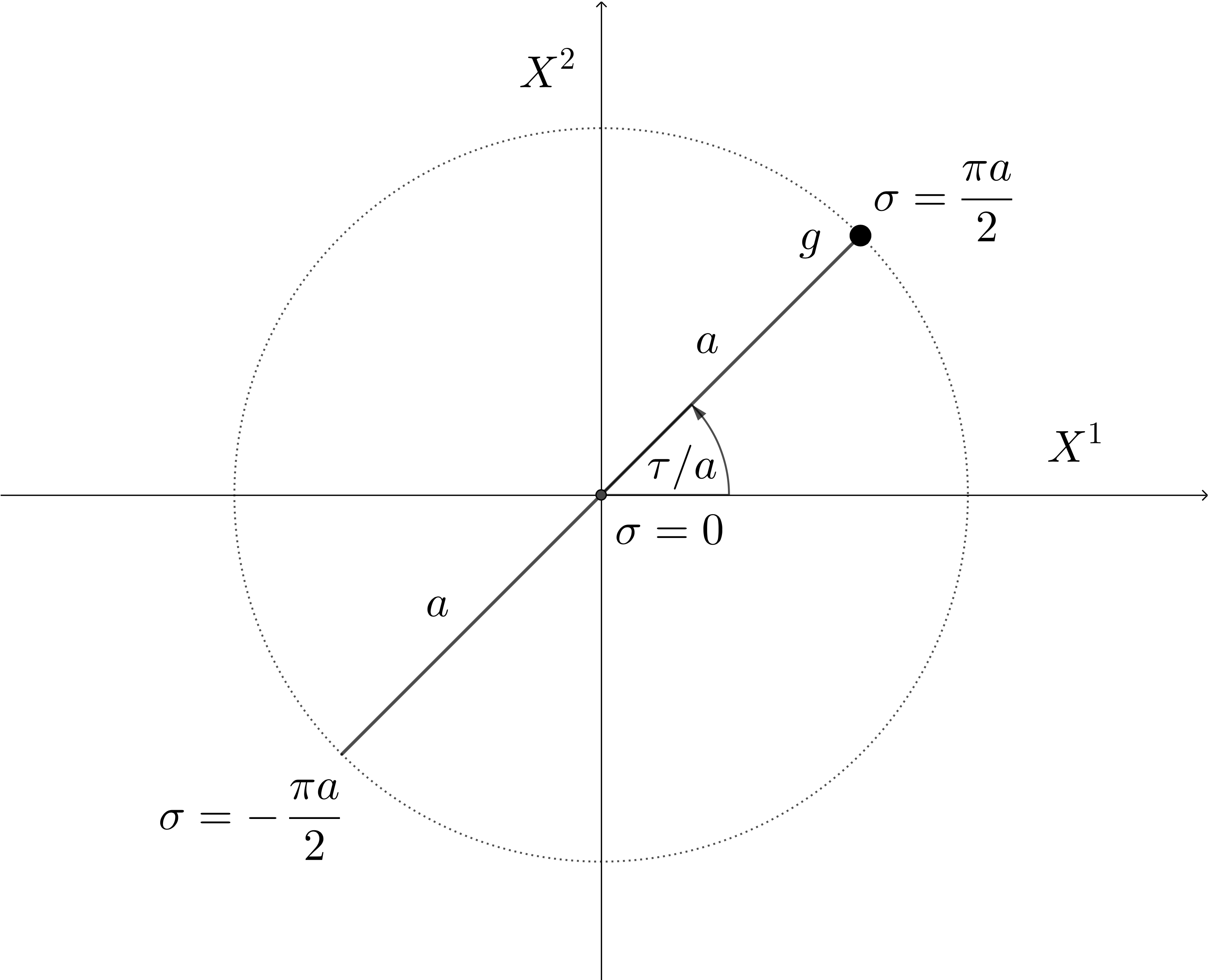
Figure 1: Rigid open string of length $2a$ with a charge $g$ at one endpoint rotating around its centre point with angular velocity $1/a$.

4.1 Leading Regge Open String Solution

The classical open string solution that corresponds to leading Regge states is a rigid string rotating around its midpoint. Since we need the string to couple to a photon, we place a charge $g$ at one endpoint, as in figure 1.

We can treat this system using classical electrodynamics and construct the current four-vector from the charge density $\rho$ and the current $\mathbf{j}$,

$$j^{\mu}(x) =\left(\rho(x),\mathbf{j}(x)\right)^{\mu}=\frac{g}{a}\delta(r-a)\delta(\phi-t/a)\delta(z)n^{\mu},$$ (40)

with $n^{\mu}=(1,\hat{\phi})=(1,-\sin(t/a),\cos(t/a),0)$. Note that we work with $c=1$. In appendix A we provide a first-principles derivation of $j^{\mu}$.

The current four-vector is analogous to the energy-momentum tensor in the gravity case, in the sense that it describes the linear coupling to the massless gauge field. More precisely, the interaction term in the Lagrangian is proportional to $h_{\mu\nu}T^{\mu\nu}$ in the gravity case and $A_{\mu}j^{\mu}$ in electromagnetism. Therefore we can construct a classical three-point amplitude in the same way as eq. (17), by contracting $j^{\mu}$ with an on-shell photon polarisation and Fourier-transforming to momentum space.

In order to construct an appropriate polarisation vector, ${\varepsilon_{k}}$, let us first consider the constraints dictated by the three-point kinematics. On these kinematics the wave number vector $k^{\mu}$ must satisfy

$$k^{2}=p_{1}\cdot k={\varepsilon_{k}}\cdot k=0,$$ (41)

where in this case $p_{1}$ is the total four-momentum of the string. We choose to work in the centre of mass frame, where the total energy of the string is $E$ and the four-momentum is $p_{1}=(E,\mathbf{0})$. In order to satisfy eq. (41) we need complexified kinematics, a suitable choice is

$$k^{\mu}=E_{\gamma}(0,i,0,-1),\qquad{\varepsilon_{k}}^{\mu}=\frac{1}{\sqrt{2}}(1,0,-1,0).$$ (42)

Given this choice we can proceed with the Fourier transform of ${\varepsilon_{k}}\cdot j$,

$$\begin{split}\mathcal{FT}[{\varepsilon_{k}}\cdot j]&=\frac{1}{2\pi a}\int d^{4}x\>e^{ik\cdot x}\>\frac{g}{a}\>{\varepsilon_{k}}\cdot n\>\delta(r-a)\delta(\phi-t/a)\delta(z)\\ &=\frac{g}{2\pi\sqrt{2}}\int_{-\pi}^{\pi}d\phi\>e^{aE_{\gamma}\cos\phi}\left(1+\cos\phi\right)\\ &=\frac{g}{\sqrt{2}}\left[I_{0}(aE_{\gamma})+I_{1}(aE_{\gamma})\right].\end{split}$$ (43)

Where we used a well known integral representation for the modified Bessel functions. Compare this result to the classical limit of the string amplitude (32) given in the previous section. While the same functions appear in both expressions, the prefactor and the arguments are written in different variables.

The rotating string is an extended object with only orbital angular momentum $J^{i}=(0,0,J_{z})$. Meanwhile, the amplitude result in (32) repackages the string as an effective point particle, with mass $m$ and intrinsic spin, $\left\langle S^{\mu}\right\rangle=(0,0,0,S_{z})$. The total energy of the effective point particle, $m$ in the centre-of-mass frame, corresponds to the total energy of the string, $E$, such that we can identify $E=m$. Likewise we can identify the spin of the effective point particle with the total angular momentum of the string, $S_{z}=J_{z}$. The total energy and total angular momentum of the string are calculated in the appendix A,

$$E=\frac{a}{2\alpha^{\prime}}\,,\hskip 22.76219ptJ_{z}=\frac{a^{2}}{4\alpha^{\prime}}.$$ (44)

Using the above and recalling that $k=E_{\gamma}(0,i,0,-1)$, we can confirm that the arguments of the Bessel functions match,

$$\frac{2k\cdot S}{m}=\frac{4E_{\gamma}\alpha^{\prime}}{a}S_{z}=aE_{\gamma}.$$ (45)

The next step is to consider the coefficient of the Bessel functions. The normalisation of the amplitude was chosen to be finite in the classical limit and it is given by $p_{1}\cdot{\varepsilon_{k}}$. In the frame specified above this reduces to the mass of the point particle $m$.

Thus we have the match between the classical open string amplitude, $\mathcal{A}_{cl.}$, computed in section 3, and the classical solution from first principles,

$$\mathcal{A}_{cl}^{string}=m\mathcal{FT}[{\varepsilon_{k}}\cdot j]=\frac{mg}{\sqrt{2}}\left[I_{0}\left(aE_{\gamma}\right)+I_{1}\left(aE_{\gamma}\right)\right].$$ (46)

4.2 Leading Regge Closed String Solution

We now move to the classical closed string configuration. The leading Regge solution now corresponds to a folded rigid string rotating around its centre point, in the same setup as figure 1. This configuration can be represented by the following stress-energy tensor

$$T^{\mu\nu} =\frac{1}{\pi\alpha^{\prime}}\frac{a\gamma(r)}{r}n^{\mu\nu}(r,\phi)\delta(z)\left[\delta(t-a\phi)+\delta(t-a\phi-a\pi)\right]\Theta(a-r),$$ (47)

with the Lorentz factor, $\gamma(r)=\left(1-\frac{r^{2}}{a^{2}}\right)^{-1/2}$, and the matrix

$$n^{\mu\nu}(r,\phi)=\begin{pmatrix}1&-\frac{r}{a}\sin{\phi}&\frac{r}{a}\cos{\phi}&0\\ -\frac{r}{a}\sin{\phi}&\frac{r^{2}}{a^{2}}-\cos^{2}{\phi}&-\frac{1}{2}\sin{2\phi}&0\\ \frac{r}{a}\cos{\phi}&-\frac{1}{2}\sin{2\phi}&\frac{r^{2}}{a^{2}}-\sin^{2}{\phi}&0\\ 0&0&0&0\end{pmatrix}.$$ (48)

The derivation of this result from the classical string solution is given in appendix A, with an explicit check that $\nabla_{\mu}T^{\mu\nu}=0$.

Now we can follow the same process as in the open string case, first we saturate the Lorentz indices of $T^{\mu\nu}$ with the massless polarisation vectors, and then we take the Fourier transform,

$$\mathcal{FT}[{\varepsilon_{k}}\cdot T\cdot{\varepsilon_{k}}] =\frac{1}{2\pi^{2}\alpha^{\prime}}\!\int\!\!d^{4}xe^{ik\cdot x}\frac{\gamma(r)}{r}{\varepsilon_{k}}\!\cdot\!n\!\cdot\!{\varepsilon_{k}}\,\delta(z)\left(\delta(t\!-\!a\phi)+\delta(t\!-\!a\phi\!-\!a\pi)\right)\Theta(a\!-\!r)$$

$$=\frac{1}{2\pi^{2}\alpha^{\prime}}\!\int drd\phi\gamma(r)\left(\frac{r}{a}+\cos{\phi}\right)^{2}e^{rE_{\gamma}\cos{\phi}}\Theta(a\!-\!r)$$

$$=\frac{m}{2}\left[I_{0}\left(\frac{aE_{\gamma}}{2}\right)+I_{1}\left(\frac{aE_{\gamma}}{2}\right)\right]^{2}$$ (49)

where we used the closed-string relation $m=E=a/\alpha^{\prime}$. In order to compare this result to eq. (3.2) we need to proceed in a similar manner to the open string case. Note that for closed strings we have $E_{\textrm{closed}}=2E_{\textrm{open}}$ and $J_{\textrm{closed}}=2J_{\textrm{open}}$, see appendix A. However the ratio $J/E$ is invariant, such that we have the same relations as in the open string case. Hence the Bessel function arguments and the prefactor in the amplitude can be expressed as

$$\frac{k\cdot S}{m}=\frac{aE_{\gamma}}{2},\qquad(p_{1}\cdot{\varepsilon_{k}})^{2}=\frac{m^{2}}{2}.$$ (50)

Thus we have the match between the classical closed string amplitude, $\mathcal{M}_{cl.}$, computed in section 3 and the classical solution from first principles,

$$\mathcal{M}_{cl}^{string}=m\mathcal{FT}[{\varepsilon_{k}}\cdot T\cdot{\varepsilon_{k}}]=\frac{m^{2}}{2}\left[I_{0}\left(\frac{aE_{\gamma}}{2}\right)+I_{1}\left(\frac{aE_{\gamma}}{2}\right)\right]^{2}.$$ (51)

5 Conclusion

In this work, we computed the classical limit of superstring amplitudes involving two massive leading Regge states and a photon or graviton. In the process, we set up a prescription for the classical limit of three-point amplitudes and discussed the importance of the spin to infinity limit to reproduce the classical spin-multipole coefficients. We found that the gauge theory and gravity results matched the electromagnetic current and stress-energy tensor obtained from fully-classical string solutions, and we highlighted the classical double copy relation between the two.

We found in section 3 that generic amplitudes do not obey the spin universality observed in the Kerr case, as shown explicitly in the string case. In particular, any amplitude for two massive states of finite spin $s$ and a photon or graviton can be expanded as a polynomial of the normalised spin operator $a^{\mu}=S^{\mu}/m$,

$$\mathcal{M}(s)\propto\sum_{n=0}^{2s}c_{n}^{(s)}\left\langle(k\cdot a_{(s)})^{n}\right\rangle,$$

such that, in general, the coefficients $c_{n}^{(s)}$ depend on the spin quantum number $s$. For example, the coefficient of the spin-quadrupole for the open string had the following functional dependence on $s$: $c_{2}^{(s)}=\frac{4s^{2}-7s+4}{2s(2s-1)}$.

This feature indicates that, in general, one cannot read off the correct classical spin multipole coefficients from finite-spin quantum amplitudes. Instead the classical coefficients correspond to the $s\to\infty$ limit of these fixed spin coefficients. Applying this approach to the leading Regge open and closed superstring amplitudes yields the following all-spin classical results,

$$\lim_{s\to\infty}\mathcal{A}(\phi^{s}(p_{1}),\phi^{s}(p_{2}),A^{+}(k)) =g\,{\varepsilon_{k}}^{+}\cdot p_{1}\left[I_{0}(2k\cdot a)+I_{1}(2k\cdot a)\right],$$

$$\lim_{s\to\infty}\mathcal{M}(\phi^{s}(p_{1}),\phi^{s}(p_{2}),h^{+}(k)) =({\varepsilon_{k}}^{+}\cdot p_{1})^{2}\left[I_{0}(k\cdot a)+I_{1}(k\cdot a)\right]^{2}.$$

Clearly these leading Regge strings do not reproduce the exponential that appears in the Kerr stress-energy tensor, instead there are modified Bessel functions appearing. We noted that the classical result inherits the double copy structure that the finite-spin string amplitudes admit at three points. This feature is also present in the Kerr case, as shown in eq. (3.2).

We were able to verify the results above by matching to purely classical calculations. The configuration associated to classical leading Regge states is known to be that of a rotating rigid string zwiebach_2004 . The open string corresponds to a string with a charged endpoint, while the closed string corresponds to a folded string coupled to gravity. We constructed the current four-vector and stress-energy tensor in the respective cases and, as was done for the Kerr case, transformed it to momentum space and contracted it with on-shell polarisation vectors corresponding to the photon/graviton. This procedure yields a classical three-point amplitude that can be compared to the infinite-spin limit results. The Bessel function structure falls out immediately and the arguments can be matched in the rest frame of the particle.

In this paper we only considered leading Regge states but one could naturally extend the analysis to other string states. It is possible that the amplitudes for a subleading Regge trajectory agree with Kerr in the spin to infinity limit. Another possibility would be to consider a superposition of string states, such as a string coherent state, and use the methods outlined in this work to try and match black-hole observables. If black-hole amplitudes were to be found within string theory, the classical limits of higher point string amplitudes could shed some light on the high-spin Compton amplitude for Kerr.

As string theory provides a consistent theory of massive interacting higher-spin particles, it was a natural setting to explore classical limits that require spin to infinity limits. However there are alternative approaches to building consistent theories of spinning particles, which have emerged from the higher-spin research community. A feasible future direction could be to explore the relation between the Kerr amplitudes and the higher-spin amplitudes that such alternative theories provide, as initiated in ref. Chiodaroli:2021eug .

Appendix A Deriving the Classical String Solutions

Let us consider a rigid open string of uniform mass density, rotating around its centre point in the same setup as figure 1. This configuration can be represented by the following string solution Ademollo:1974te ; Lust1989 ; zwiebach_2004 :

$$X^{0}=\tau,$$

$$X^{1}=a\cos{\frac{\tau}{a}}\sin{\frac{\sigma}{a}},$$

$$X^{2}=a\sin{\frac{\tau}{a}}\sin{\frac{\sigma}{a}},$$

$$X^{3}=0,$$ (52)

with $\sigma\in[-\frac{\pi a}{2},\frac{\pi a}{2}]$ and $\tau\in(-\infty,\infty)$. The extension to the closed string is simply achieved by extending the range of $\sigma$ to $[-\pi a,\pi a]$ and it describes a rigid folded string rotating around its centre point in the same fashion. It is convenient to express this in polar coordinates; in order to keep $r>0$ we define different coordinates on the two branches of the string. The corresponding polar coordinates for the open string are

	$\sigma\in\left[0,\frac{\pi a}{2}\right]$	$\sigma\in\left[-\frac{\pi a}{2},0\right]$
$r^{\prime}$	$a\sin\frac{\sigma}{a}$	$-a\sin\frac{\sigma}{a}$
$\phi^{\prime}$	$\frac{\tau}{a}$	$\frac{\tau}{a}-\pi$

while the closed string requires the definitions on the additional domains

	$\sigma\in[\frac{\pi a}{2},\pi a]$	$\sigma\in[-\pi a,-\frac{\pi a}{2}]$
$r^{\prime}$	$a\sin\left(\pi-\frac{\sigma}{a}\right)$	$a\sin\left(\pi+\frac{\sigma}{a}\right)$
$\phi^{\prime}$	$\frac{\tau}{a}$	$\frac{\tau}{a}-\pi$

Below we study the coupling of this solution to the electromagnetic and gravitational fields.

A.1 Coupling to Gravity

We consider the string action in a curved background

$$S=\frac{1}{4\pi\alpha^{\prime}}\int d^{4}yd^{2}\sigma\delta^{4}(y-X(\sigma))\partial_{a}X^{\mu}\partial^{a}X^{\nu}g_{\mu\nu}(y),$$ (53)

and hence we can compute the linearised energy-momentum tensor

$$T^{\mu\nu}=\frac{2}{\sqrt{-g}}\frac{\delta S}{\delta g_{\mu\nu}(y)}\Big{|}_{g=\eta}=\frac{1}{2\pi\alpha^{\prime}}\int d^{2}\sigma\delta^{4}(y-X(\sigma))\partial_{a}X^{\mu}\partial^{a}X^{\nu},$$ (54)

where

$$\partial_{a}X^{\mu}\partial^{a}X^{\nu}=\begin{pmatrix}1&-S_{\tau}S_{\sigma}&C_{\tau}S_{\sigma}&0\\ -S_{\tau}S_{\sigma}&S_{\tau}^{2}S_{\sigma}^{2}-C_{\tau}^{2}C_{\sigma}^{2}&-S_{\tau}C_{\tau}&0\\ C_{\tau}S_{\sigma}&-S_{\tau}C_{\tau}&C_{\tau}^{2}S_{\sigma}^{2}-S_{\tau}^{2}C_{\sigma}^{2}&0\\ 0&0&0&0\end{pmatrix},$$

$$\delta^{4}(y-X(\sigma))=\delta(t-\tau)\delta(z)\delta(x-aC_{\tau}S_{\sigma})\delta(y-aS_{\tau}S_{\sigma})$$ (55)

and we have used $C_{\alpha}\equiv\cos{\frac{\alpha}{a}},S_{\alpha}\equiv\sin{\frac{\alpha}{a}}$ and $y^{\mu}=(t,x,y,z)$.

Now let us integrate out the worldsheet coordinates $\{\sigma,\tau\}$. The form of $T^{\mu\nu}$ above suggests doing the integral in polar coordinates, which will introduce multiple Jacobian factors. As well as the measure, the delta function $\delta^{4}(y-X(\sigma))$ will pick up a Jacobian factor due to the change of variables,

$$\delta^{4}(y-X(\sigma)) =\delta(t-\tau)\delta(z)\delta(x-X^{1})\delta(y-X^{2})$$

$$=\frac{1}{|\mathcal{J}(r^{\prime},\phi^{\prime};X^{1},X^{2})|}\delta(t-\tau)\delta(z)\delta(r-r^{\prime})\delta(\phi-\phi^{\prime})$$ (56)

where $X^{1}=r^{\prime}\cos\phi^{\prime}$, $X^{2}=r^{\prime}\sin\phi^{\prime}$. The Jacobian factors needed are

$$|\mathcal{J}(r^{\prime},\phi^{\prime};X^{1},X^{2})|=r^{\prime},$$

$$|\mathcal{J}(r^{\prime},\phi^{\prime};\sigma,\tau)|=a\gamma(r^{\prime})\,$$ (57)

where $\gamma(r^{\prime})=\left(1-\frac{{r^{\prime}}^{2}}{a^{2}}\right)^{-1/2}$ is the Lorentz factor. Thus the integral can be simplified to

$$T^{\mu\nu}=\frac{1}{2\pi\alpha^{\prime}}\int dr^{\prime}d\phi^{\prime}\frac{|\mathcal{J}(r^{\prime},\phi^{\prime};\sigma,\tau)|}{|\mathcal{J}(r^{\prime},\phi^{\prime};x^{\prime},y^{\prime})|}\left[\delta(t-a\phi^{\prime})+\delta(t-a\phi^{\prime}-a\pi)\right]\\ \times\delta(z)\delta(r-r^{\prime})\delta(\phi-\phi^{\prime})\partial_{a}X^{\mu}\partial^{a}X^{\nu}.$$ (58)

Performing the integral we get the expression

$$T^{\mu\nu}=\frac{N_{\text{string}}}{2\pi\alpha^{\prime}}\frac{a\gamma(r)}{r}\left[\delta(t-a\phi)+\delta(t-a\phi-a\pi)\right]\Theta(a-r)\delta(z)n^{\mu\nu},$$ (59)

where

$$n^{\mu\nu}(r,\phi)=\begin{pmatrix}1&-\frac{r}{a}\sin{\phi}&\frac{r}{a}\cos{\phi}&0\\ -\frac{r}{a}\sin{\phi}&\frac{r^{2}}{a^{2}}-\cos^{2}{\phi}&-\frac{1}{2}\sin{2\phi}&0\\ \frac{r}{a}\cos{\phi}&-\frac{1}{2}\sin{2\phi}&\frac{r^{2}}{a^{2}}-\sin^{2}{\phi}&0\\ 0&0&0&0\end{pmatrix}$$ (60)

and we have introduced the normalisation $N_{\text{string}}$ which is equal to $1$ in the open case and $2$ in the closed case, since the enlarged $\sigma$ domain effectively corresponds to summing two open strings together.

Given $T^{\mu\nu}$ we can now calculate the total energy $E$,

$$E =\int d^{3}xT^{tt}$$

$$=\frac{N_{\text{string}}}{2\pi\alpha^{\prime}}\int rdrd\phi dz\frac{a\gamma(r)}{r}\left[\delta(t-a\phi)+\delta(t-a\phi-a\pi)\right]\Theta(a-r)\delta(z)$$

$$=\frac{N_{\text{string}}}{\pi\alpha^{\prime}}\int_{0}^{a}rdr\frac{\gamma(r)}{r}=N_{\text{string}}\frac{a}{2\alpha^{\prime}}.$$ (61)

We can also compute the total angular momentum $J$. Since the string is rotating in the $z=0$ plane the angular momentum is only in the $z$ direction, $J=J_{z}$,

$$J =\int d^{3}x\left(xT^{ty}-yT^{tx}\right)$$

$$=\frac{N_{\text{string}}}{2\pi\alpha^{\prime}}\int rdrd\phi dz\left(r\gamma(r)\right)\left[\delta(t-a\phi)+\delta(t-a\phi-a\pi)\right]\Theta(a-r)\delta(z)$$

$$=\frac{N_{\text{string}}}{2\pi\alpha^{\prime}}\int_{0}^{a}dr\frac{r^{2}\gamma(r)}{a}=N_{\text{string}}\frac{a^{2}}{4\alpha^{\prime}}.$$ (62)

The results for $E$ and $J$ above can be used to recover the leading Regge trajectory relation at the classical level. For instance for the open string we have

$$J=\alpha^{\prime}E^{2}$$ (63)

which is analogous to eq. (23) in the large spin limit, suggesting that this classical string configuration indeed corresponds to the classical limit of leading Regge string amplitudes.

Another important check is that this energy-momentum tensor in conserved, $\nabla_{\mu}T^{\mu\nu}=0$. This is easier to show if we convert the tensor from Cartesian coordinates $x^{\mu}=(t,x,y,z)$ to cylindrical polar coordinates $x^{\prime\mu}=(t,r,\phi,z)$,

$$n^{\mu\nu}_{pol}=\frac{\partial x^{\prime\mu}}{\partial x^{\alpha}}\frac{\partial x^{\prime\nu}}{\partial x^{\beta}}n^{\alpha\beta}\\ =\begin{pmatrix}1&0&\frac{1}{a}&0\\ 0&-1+\frac{r^{2}}{a^{2}}&0&0\\ \frac{1}{a}&0&\frac{1}{a^{2}}&0\\ 0&0&0&0\end{pmatrix}.$$ (64)

Note that in this set of coordinates we have some non-vanishing Christoffel symbols, namely $\Gamma^{r}_{\phi\phi}=-r$ and $\Gamma^{\phi}_{r\phi}=\Gamma^{\phi}_{\phi r}=1/r$. Hence we get,

$$\int d^{4}xf(x)\nabla_{\mu}T^{\mu\nu}=\int d^{4}xf(x)\begin{pmatrix}\partial_{t}T^{tt}+\partial_{\phi}T^{\phi t}\\ \partial_{r}T^{rr}+\frac{1}{r}T^{rr}-rT^{\phi\phi}\\ \partial_{t}T^{t\phi}+\partial_{\phi}T^{\phi\phi}\\ 0\end{pmatrix}.$$ (65)

Let us begin with the $t$ component. We get

$$\int d^{4}xf(x)\nabla_{\mu}T^{\mu t}\\ =\frac{aN_{\text{string}}}{2\pi\alpha^{\prime}}\int d^{4}xf(x)\frac{\gamma(r)}{r}\delta(z)\Theta(a-r)\left(\partial_{t}\delta(t-a\phi)+\frac{1}{a}\partial_{\phi}\delta(t-a\phi)\right).$$ (66)

This is equal to zero due to the identity $\partial_{\phi}\delta(t-a\phi)=-a\partial_{t}\delta(t-a\phi)$. Note that we have omitted the term proportional to $\delta(t-a\phi-a\pi)$ for convenience, but it can be obtained from the above by shifting $\phi\to\phi+\pi$ and the same argument applies. Next we consider the $\phi$ component,

$$\int d^{4}xf(x)\nabla_{\mu}T^{\mu\phi}\\ =\frac{aN_{\text{string}}}{2\pi\alpha^{\prime}}\int d^{4}xf(x)\frac{\gamma(r)}{r}\delta(z)\Theta(a-r)\left(\frac{1}{a}\partial_{t}\delta(t-a\phi)+\frac{1}{a^{2}}\partial_{\phi}\delta(t-a\phi)\right).$$ (67)

This is just a rescaling of eq. (66), and hence it vanishes for the same reason. The $r$ component is slightly more involved, and it is given by

$$\int d^{4}xf(x)T^{\mu r} =\frac{aN_{\text{string}}}{2\pi\alpha^{\prime}}\!\int d^{4}xf(x)\delta(t\!-\!a\phi)\delta(z)\left\{-\partial_{r}\left(\frac{\Theta(a\!-\!r)}{r\gamma(r)}\right)-\Theta(a\!-\!r)\frac{\gamma(r)}{r^{2}}\right\}$$

$$=\frac{aN_{\text{string}}}{2\pi\alpha^{\prime}}\!\int d^{4}xf(x)\delta(t\!-\!a\phi)\delta(z)\frac{1}{r\gamma(r)}\delta(a\!-\!r)$$ (68)

where we have used $\partial_{r}\Theta(a-r)=-\delta(a-r)$. Since $(\gamma(a))^{-1}=0$, the integrand vanishes on the support of the delta function $\delta(a-r)$. As before, the same argument applies for the term proportional to $\delta(t-a\phi-a\pi)$. Since all components are zero, the identity $\nabla_{\mu}T^{\mu\nu}=0$ is verified.

A.2 Coupling to Electromagnetism

The coupling of an open string to the electromagnetic field is given by the following action Tong:2009np ,

$$S_{EM}=ig\int d^{2}\sigma\delta\left(\sigma-\frac{\pi a}{2}\right)A^{a}_{\mu}(X)\dot{X}^{\mu}$$ (69)

where $g$ is the charge. Note that we chose to place it only at one endpoint, $\sigma=\pi a/2$, but in principle we could add a similar term at $\sigma=-\pi a/2$. The string solution gives

$$\begin{split}&X^{\mu}(\tau,\pi a/2)=\left(\tau,a\cos{\frac{\tau}{a}},a\sin{\frac{\tau}{a}},0\right),\\ &\dot{X}^{\mu}(\tau,\pi a/2)=\left(1,-\sin{\frac{\tau}{a}},\cos{\frac{\tau}{a}},0\right)\equiv n^{\mu}(\tau/a).\end{split}$$ (70)

From this we can derive the electromagnetic current,

$$j^{\mu}(y) =-i\frac{\partial S_{EM}}{\partial A_{\mu}(y)}=g\int d\tau\,n^{\mu}(\tau/a)\delta(\tau-t)\delta\left(x-a\cos{\frac{\tau}{a}}\right)\delta\left(y-a\sin{\frac{\tau}{a}}\right)\delta(z)$$

$$=g\,n^{\mu}(t/a)\delta\left(x-a\cos{\frac{t}{a}}\right)\delta\left(y-a\sin{\frac{t}{a}}\right)\delta(z)$$

$$=\frac{g}{a}n^{\mu}(\phi)\delta(r-a)\delta\left(\phi-\frac{t}{a}\right)\delta(z)$$ (71)

where we have chosen the normalisation such that $\int d^{3}xj^{0}(x)=g$. Similarly to the closed string case, we can check the conservation condition $\nabla_{\mu}j^{\mu}=0$ by integrating it against an arbitrary function $f(x)$. It is again convenient to rewrite $n^{\mu}$ in cylindrical polar coordinates,

$$n^{\mu}_{pol}=\left(1,0,\frac{1}{r},0\right).$$ (72)

Hence we have

$$\int d^{4}xf(x)\nabla_{\mu}j^{\mu}=\frac{cg}{a}\int d^{4}xf(x)\delta(r-a)\delta(z)\left\{\partial_{t}\delta\left(\phi-\frac{t}{a}\right)+\frac{1}{a}\partial_{\phi}\delta\left(\phi-\frac{t}{a}\right)\right\}$$ (73)

where in this case $\nabla_{\mu}j^{\mu}=\partial_{\mu}j^{\mu}$ since there are no non-zero Christoffel symbols contributing. This integral vanishes because of the identity $\partial_{\phi}\delta(\phi-t/a)=-a\partial_{t}\delta(\phi-t/a)$, which we used already in eq. (66).

References

- (1) V. Vaidya, Gravitational spin Hamiltonians from the S matrix, Phys. Rev. D 91 (2015) 024017 [1410.5348].
- (2) N. Arkani-Hamed, T.-C. Huang and Y.-t. Huang, Scattering amplitudes for all masses and spins, JHEP 11 (2021) 070 [1709.04891].
- (3) J. Vines, Scattering of two spinning black holes in post-Minkowskian gravity, to all orders in spin, and effective-one-body mappings, Class. Quant. Grav. 35 (2018) 084002 [1709.06016].
- (4) A. Guevara, Holomorphic Classical Limit for Spin Effects in Gravitational and Electromagnetic Scattering, JHEP 04 (2019) 033 [1706.02314].
- (5) A. Guevara, A. Ochirov and J. Vines, Scattering of Spinning Black Holes from Exponentiated Soft Factors, JHEP 09 (2019) 056 [1812.06895].
- (6) M.-Z. Chung, Y.-T. Huang, J.-W. Kim and S. Lee, The simplest massive S-matrix: from minimal coupling to Black Holes, JHEP 04 (2019) 156 [1812.08752].
- (7) A. Guevara, A. Ochirov and J. Vines, Black-hole scattering with general spin directions from minimal-coupling amplitudes, Phys. Rev. D 100 (2019) 104024 [1906.10071].
- (8) M.-Z. Chung, Y.-t. Huang, J.-W. Kim and S. Lee, Complete Hamiltonian for spinning binary systems at first post-Minkowskian order, JHEP 05 (2020) 105 [2003.06600].
- (9) H. Kawai, D.C. Lewellen and S.H.H. Tye, A Relation Between Tree Amplitudes of Closed and Open Strings, Nucl. Phys. B 269 (1986) 1.
- (10) Z. Bern, J.J.M. Carrasco and H. Johansson, New Relations for Gauge-Theory Amplitudes, Phys. Rev. D 78 (2008) 085011 [0805.3993].
- (11) Z. Bern, J.J.M. Carrasco and H. Johansson, Perturbative Quantum Gravity as a Double Copy of Gauge Theory, Phys. Rev. Lett. 105 (2010) 061602 [1004.0476].
- (12) Z. Bern, J.J. Carrasco, M. Chiodaroli, H. Johansson and R. Roiban, The Duality Between Color and Kinematics and its Applications, 1909.01358.
- (13) H. Johansson and A. Ochirov, Color-Kinematics Duality for QCD Amplitudes, JHEP 01 (2016) 170 [1507.00332].
- (14) A. Ochirov, Helicity amplitudes for QCD with massive quarks, JHEP 04 (2018) 089 [1802.06730].
- (15) H. Johansson and A. Ochirov, Double copy for massive quantum particles with spin, JHEP 09 (2019) 040 [1906.12292].
- (16) M.-Z. Chung, Y.-T. Huang and J.-W. Kim, Classical potential for general spinning bodies, JHEP 09 (2020) 074 [1908.08463].
- (17) Y.F. Bautista and A. Guevara, On the double copy for spinning matter, JHEP 11 (2021) 184 [1908.11349].
- (18) N. Arkani-Hamed, Y.-t. Huang and D. O’Connell, Kerr black holes as elementary particles, JHEP 01 (2020) 046 [1906.10100].
- (19) A. Edison and F. Teng, Efficient Calculation of Crossing Symmetric BCJ Tree Numerators, JHEP 12 (2020) 138 [2005.03638].
- (20) L.A. Johnson, C.R.T. Jones and S. Paranjape, Constraints on a Massive Double-Copy and Applications to Massive Gravity, JHEP 02 (2021) 148 [2004.12948].
- (21) A. Momeni, J. Rumbutis and A.J. Tolley, Kaluza-Klein from colour-kinematics duality for massive fields, JHEP 08 (2021) 081 [2012.09711].
- (22) A. Momeni, J. Rumbutis and A.J. Tolley, Massive Gravity from Double Copy, JHEP 12 (2020) 030 [2004.07853].
- (23) K. Haddad and A. Helset, The double copy for heavy particles, Phys. Rev. Lett. 125 (2020) 181603 [2005.13897].
- (24) W.T. Emond, Y.-T. Huang, U. Kol, N. Moynihan and D. O’Connell, Amplitudes from Coulomb to Kerr-Taub-NUT, JHEP 05 (2022) 055 [2010.07861].
- (25) N.E.J. Bjerrum-Bohr, T.V. Brown and H. Gomez, Scattering of Gravitons and Spinning Massive States from Compact Numerators, JHEP 04 (2021) 234 [2011.10556].
- (26) A. Brandhuber, G. Chen, G. Travaglini and C. Wen, A new gauge-invariant double copy for heavy-mass effective theory, JHEP 07 (2021) 047 [2104.11206].
- (27) R. Monteiro, D. O’Connell and C.D. White, Black holes and the double copy, JHEP 12 (2014) 056 [1410.0239].
- (28) Y.-T. Huang, U. Kol and D. O’Connell, Double copy of electric-magnetic duality, Phys. Rev. D 102 (2020) 046005 [1911.06318].
- (29) M.-Z. Chung, Y.-T. Huang and J.-W. Kim, Kerr-Newman stress-tensor from minimal coupling, JHEP 12 (2020) 103 [1911.12775].
- (30) A. Guevara, B. Maybee, A. Ochirov, D. O’Connell and J. Vines, A worldsheet for Kerr, JHEP 03 (2021) 201 [2012.11570].
- (31) B. Maybee, D. O’Connell and J. Vines, Observables and amplitudes for spinning particles and black holes, JHEP 12 (2019) 156 [1906.09260].
- (32) R. Aoude, K. Haddad and A. Helset, On-shell heavy particle effective theories, JHEP 05 (2020) 051 [2001.09164].
- (33) R. Aoude and A. Ochirov, Classical observables from coherent-spin amplitudes, JHEP 10 (2021) 008 [2108.01649].
- (34) B.R. Holstein and A. Ross, Spin Effects in Long Range Electromagnetic Scattering, 0802.0715.
- (35) B.R. Holstein and A. Ross, Spin Effects in Long Range Gravitational Scattering, 0802.0716.
- (36) R. Aoude, M.-Z. Chung, Y.-t. Huang, C.S. Machado and M.-K. Tam, Silence of Binary Kerr Black Holes, Phys. Rev. Lett. 125 (2020) 181602 [2007.09486].
- (37) B.-T. Chen, M.-Z. Chung, Y.-t. Huang and M.K. Tam, Minimal spin deflection of Kerr-Newman and supersymmetric black hole, JHEP 10 (2021) 011 [2106.12518].
- (38) K. Haddad, Exponentiation of the leading eikonal phase with spin, Phys. Rev. D 105 (2022) 026004 [2109.04427].
- (39) Z. Bern, A. Luna, R. Roiban, C.-H. Shen and M. Zeng, Spinning black hole binary dynamics, scattering amplitudes, and effective field theory, Phys. Rev. D 104 (2021) 065014 [2005.03071].
- (40) Z. Liu, R.A. Porto and Z. Yang, Spin effects in the effective field theory approach to post-minkowskian conservative dynamics, Journal of High Energy Physics 2021 (2021) .
- (41) G.U. Jakobsen, G. Mogull, J. Plefka and J. Steinhoff, Gravitational Bremsstrahlung and Hidden Supersymmetry of Spinning Bodies, Phys. Rev. Lett. 128 (2022) 011101 [2106.10256].
- (42) G.U. Jakobsen and G. Mogull, Conservative and Radiative Dynamics of Spinning Bodies at Third Post-Minkowskian Order Using Worldline Quantum Field Theory, Phys. Rev. Lett. 128 (2022) 141102 [2201.07778].
- (43) M.M. Riva, F. Vernizzi and L.K. Wong, Gravitational Bremsstrahlung from Spinning Binaries in the Post-Minkowskian Expansion, 2205.15295.
- (44) N. Siemonsen and J. Vines, Test black holes, scattering amplitudes and perturbations of Kerr spacetime, Phys. Rev. D 101 (2020) 064066 [1909.07361].
- (45) P.H. Damgaard, K. Haddad and A. Helset, Heavy Black Hole Effective Theory, JHEP 11 (2019) 070 [1908.10308].
- (46) D. Kosmopoulos and A. Luna, Quadratic-in-spin Hamiltonian at (G2) from scattering amplitudes, JHEP 07 (2021) 037 [2102.10137].
- (47) W.-M. Chen, M.-Z. Chung, Y.-t. Huang and J.-W. Kim, The 2PM Hamiltonian for binary Kerr to quartic in spin, 2111.13639.
- (48) G. Menezes and M. Sergola, NLO deflections for spinning particles and Kerr black holes, 2205.11701.
- (49) F. Febres Cordero, M. Kraus, G. Lin, M.S. Ruf and M. Zeng, Conservative Binary Dynamics with a Spinning Black Hole at from Scattering Amplitudes, 2205.07357.
- (50) R. Aoude, K. Haddad and A. Helset, Tidal effects for spinning particles, JHEP 03 (2021) 097 [2012.05256].
- (51) Z. Bern, J. Parra-Martinez, R. Roiban, E. Sawyer and C.-H. Shen, Leading Nonlinear Tidal Effects and Scattering Amplitudes, JHEP 05 (2021) 188 [2010.08559].
- (52) G. Mogull, J. Plefka and J. Steinhoff, Classical black hole scattering from a worldline quantum field theory, JHEP 02 (2021) 048 [2010.02865].
- (53) M. Accettulli Huber, A. Brandhuber, S. De Angelis and G. Travaglini, From amplitudes to gravitational radiation with cubic interactions and tidal effects, Phys. Rev. D 103 (2021) 045015 [2012.06548].
- (54) A. Cristofoli, R. Gonzo, D.A. Kosower and D. O’Connell, Waveforms from Amplitudes, 2107.10193.
- (55) E. Herrmann, J. Parra-Martinez, M.S. Ruf and M. Zeng, Gravitational Bremsstrahlung from Reverse Unitarity, Phys. Rev. Lett. 126 (2021) 201602 [2101.07255].
- (56) S. Mougiakakos, M.M. Riva and F. Vernizzi, Gravitational Bremsstrahlung in the post-Minkowskian effective field theory, Phys. Rev. D 104 (2021) 024041 [2102.08339].
- (57) Y.F. Bautista and N. Siemonsen, Post-Newtonian waveforms from spinning scattering amplitudes, JHEP 01 (2022) 006 [2110.12537].
- (58) F. Alessio and P. Di Vecchia, Radiation reaction for spinning black-hole scattering, 2203.13272.
- (59) X. Bekaert, N. Boulanger, A. Campoleoni, M. Chiodaroli, D. Francia, M. Grigoriev et al., Snowmass White Paper: Higher Spin Gravity and Higher Spin symmetry, 2205.01567.
- (60) R. Britto, F. Cachazo and B. Feng, New recursion relations for tree amplitudes of gluons, Nucl. Phys. B 715 (2005) 499 [hep-th/0412308].
- (61) R. Britto, F. Cachazo, B. Feng and E. Witten, Direct proof of tree-level recursion relation in Yang-Mills theory, Phys. Rev. Lett. 94 (2005) 181602 [hep-th/0501052].
- (62) R. Aoude, K. Haddad and A. Helset, Searching for Kerr in the 2PM amplitude, 2203.06197.
- (63) Z. Bern, D. Kosmopoulos, A. Luna, R. Roiban and F. Teng, Binary Dynamics Through the Fifth Power of Spin at , 2203.06202.
- (64) R. Aoude, K. Haddad and A. Helset, Classical gravitational spinning-spinless scattering at , 2205.02809.
- (65) W.-M. Chen, M.-Z. Chung, Y.-t. Huang and J.-W. Kim, Lense-Thirring effects from on-shell amplitudes, 2205.07305.
- (66) M. Chiodaroli, H. Johansson and P. Pichini, Compton black-hole scattering for s 5/2, JHEP 02 (2022) 156 [2107.14779].
- (67) A. Falkowski and C.S. Machado, Soft Matters, or the Recursions with Massive Spinors, JHEP 05 (2021) 238 [2005.08981].
- (68) Y.F. Bautista, A. Guevara, C. Kavanagh and J. Vines, From Scattering in Black Hole Backgrounds to Higher-Spin Amplitudes: Part I, 2107.10179.
- (69) I. Koh, W. Troost and A. Van Proeyen, Covariant higher spin vertex operators in the ramond sector, Nuclear Physics B 292 (1987) 201.
- (70) N. Berkovits and O. Chandia, Massive superstring vertex operator in D = 10 superspace, JHEP 08 (2002) 040 [hep-th/0204121].
- (71) A. Hanany, D. Forcella and J. Troost, The Covariant perturbative string spectrum, Nucl. Phys. B 846 (2011) 212 [1007.2622].
- (72) M. Bianchi, L. Lopez and R. Richter, On stable higher spin states in Heterotic String Theories, JHEP 03 (2011) 051 [1010.1177].
- (73) D. Lüst, N. Mekareeya, O. Schlotterer and A. Thomson, Refined Partition Functions for Open Superstrings with 4, 8 and 16 Supercharges, Nucl. Phys. B 876 (2013) 55 [1211.1018].
- (74) J.-C. Lee and Y. Mitsuka, Recurrence relations of Kummer functions and Regge string scattering amplitudes, JHEP 04 (2013) 082 [1212.6915].
- (75) W.-Z. Feng, D. Lust and O. Schlotterer, Massive Supermultiplets in Four-Dimensional Superstring Theory, Nucl. Phys. B 861 (2012) 175 [1202.4466].
- (76) C.-H. Fu, J.-C. Lee, C.-I. Tan and Y. Yang, Recurrence relations of higher spin BPST vertex operators for open strings, Phys. Rev. D 88 (2013) 046004 [1304.6948].
- (77) D. Polyakov, Higher spins and open strings: Quartic interactions, Phys. Rev. D 83 (2011) 046005.
- (78) W.-Z. Feng, D. Lust, O. Schlotterer, S. Stieberger and T.R. Taylor, Direct Production of Lightest Regge Resonances, Nucl. Phys. B 843 (2011) 570 [1007.5254].
- (79) O. Schlotterer, SUSY multiplets at first mass level in D=4 superstring compactifications, Nucl. Phys. B Proc. Suppl. 216 (2011) 265.
- (80) W.-Z. Feng and T.R. Taylor, Higher Level String Resonances in Four Dimensions, Nucl. Phys. B 856 (2012) 247 [1110.1087].
- (81) R.H. Boels, Three particle superstring amplitudes with massive legs, JHEP 06 (2012) 026 [1201.2655].
- (82) M. Tsulaia, On Tensorial Spaces and BCFW Recursion Relations for Higher Spin Fields, Int. J. Mod. Phys. A 27 (2012) 1230011 [1202.6309].
- (83) W.-Z. Feng, Physics of massive superstrings, Ph.D. thesis, Northeastern U., 2012.
- (84) R.H. Boels and T. Hansen, String theory in target space, JHEP 06 (2014) 054 [1402.6356].
- (85) J.A. Minahan and R. Pereira, Three-point correlators from string amplitudes: Mixing and Regge spins, JHEP 04 (2015) 134 [1410.4746].
- (86) T. Hansen, Dissecting CFT Correlators and String Amplitudes: Conformal Blocks and On-Shell Recursion for General Tensor Fields, Ph.D. thesis, Hamburg U., 2015. 10.3204/DESY-THESIS-2015-026.
- (87) S. Chakrabarti, S.P. Kashyap and M. Verma, Amplitudes Involving Massive States Using Pure Spinor Formalism, JHEP 12 (2018) 071 [1808.08735].
- (88) T. Lee and H. Park, Graviton and Massive Symmetric Rank-Two Tensor in String Theory, Acta Phys. Polon. Supp. 13 (2020) 303 [1909.08516].
- (89) D.J. Gross and V. Rosenhaus, Chaotic scattering of highly excited strings, JHEP 05 (2021) 048 [2103.15301].
- (90) R.L. Jusinskas, Asymmetrically twisted strings, Phys. Lett. B 829 (2022) 137090 [2108.13426].
- (91) M. Guillen, H. Johansson, R.L. Jusinskas and O. Schlotterer, Scattering Massive String Resonances through Field-Theory Methods, Phys. Rev. Lett. 127 (2021) 051601 [2104.03314].
- (92) I. Giannakis, J.T. Liu and M. Porrati, Massive higher spin states in string theory and the principle of equivalence, Phys. Rev. D 59 (1999) 104013 [hep-th/9809142].
- (93) I.L. Buchbinder, V.A. Krykhtin and V.D. Pershin, On consistent equations for massive spin two field coupled to gravity in string theory, Phys. Lett. B 466 (1999) 216 [hep-th/9908028].
- (94) I.L. Buchbinder, D.M. Gitman, V.A. Krykhtin and V.D. Pershin, Equations of motion for massive spin-2 field coupled to gravity, Nucl. Phys. B 584 (2000) 615 [hep-th/9910188].
- (95) I.L. Buchbinder and V.D. Pershin, Gravitational interaction of higher spin massive fields and string theory, in Conference on Geometrical Aspects of Quantum Fields, pp. 11–30, 4, 2000, DOI [hep-th/0009026].
- (96) G. Velo and D. Zwanziger, Propagation and quantization of rarita-schwinger waves in an external electromagnetic potential, Phys. Rev. 186 (1969) 1337.
- (97) G. Velo and D. Zwanzinger, Noncausality and other defects of interaction lagrangians for particles with spin one and higher, Phys. Rev. 188 (1969) 2218.
- (98) M. Taronna, Higher Spins and String Interactions, other thesis, Scuola Normale Superiore - PISA, 5, 2010, [1005.3061].
- (99) E. Joung, L. Lopez and M. Taronna, On the cubic interactions of massive and partially-massless higher spins in (A)dS, JHEP 07 (2012) 041 [1203.6578].
- (100) M. Taronna, Higher-Spin Interactions: three-point functions and beyond, Ph.D. thesis, Pisa, Scuola Normale Superiore, 2012. 1209.5755.
- (101) R. Rahman and M. Taronna, From Higher Spins to Strings: A Primer, 1512.07932.
- (102) R. Marotta, M. Taronna and M. Verma, Revisiting higher-spin gyromagnetic couplings, JHEP 06 (2021) 168 [2102.13180].
- (103) D.J. Gross, High-Energy Symmetries of String Theory, Phys. Rev. Lett. 60 (1988) 1229.
- (104) J.-C. Lee, Spontaneously broken symmetry in string theory, Phys. Lett. B 326 (1994) 79 [hep-th/0503056].
- (105) C.-T. Chan and J.-C. Lee, Stringy symmetries and their high-energy limits, Phys. Lett. B 611 (2005) 193 [hep-th/0312226].
- (106) C.-T. Chan, P.-M. Ho and J.-C. Lee, Ward identities and high-energy scattering amplitudes in string theory, Nucl. Phys. B 708 (2005) 99 [hep-th/0410194].
- (107) C.-T. Chan, P.-M. Ho, J.-C. Lee, S. Teraguchi and Y. Yang, Solving all 4-point correlation functions for bosonic open string theory in the high energy limit, Nucl. Phys. B 725 (2005) 352 [hep-th/0504138].
- (108) C.-T. Chan, P.-M. Ho, J.-C. Lee, S. Teraguchi and Y. Yang, High-energy zero-norm states and symmetries of string theory, Phys. Rev. Lett. 96 (2006) 171601 [hep-th/0505035].
- (109) C.-T. Chan, J.-C. Lee and Y. Yang, Scatterings of Massive String States from D-brane and Their Linear Relations at High Energies, Nucl. Phys. B 764 (2007) 1 [hep-th/0610062].
- (110) D. Polyakov, Interactions of Massless Higher Spin Fields From String Theory, Phys. Rev. D 82 (2010) 066005 [0910.5338].
- (111) D. Polyakov, Gravitational Couplings of Higher Spins from String Theory, Int. J. Mod. Phys. A 25 (2010) 4623 [1005.5512].
- (112) A. Fotopoulos and M. Tsulaia, On the Tensionless Limit of String theory, Off - Shell Higher Spin Interaction Vertices and BCFW Recursion Relations, JHEP 11 (2010) 086 [1009.0727].
- (113) M. Bianchi and P. Teresi, Scattering higher spins off D-branes, JHEP 01 (2012) 161 [1108.1071].
- (114) J.-C. Lee and Y. Yang, Overview of High Energy String Scattering Amplitudes and Symmetries of String Theory, Symmetry 11 (2019) 1045 [1907.12810].
- (115) A. Sagnotti and M. Taronna, String Lessons for Higher-Spin Interactions, Nucl. Phys. B 842 (2011) 299 [1006.5242].
- (116) O. Schlotterer, Higher Spin Scattering in Superstring Theory, Nucl. Phys. B 849 (2011) 433 [1011.1235].
- (117) M. Ademollo, A. D’Adda, R. D’Auria, E. Napolitano, S. Sciuto, P. Di Vecchia et al., Theory of an interacting string and dual resonance model, Nuovo Cim. A 21 (1974) 77.
- (118) D. Lust, The classical bosonic string, in Lectures on String Theory, (Berlin, Heidelberg), pp. 5–30, Springer Berlin Heidelberg (1989), DOI.
- (119) B. Zwiebach, A First Course in String Theory, Cambridge University Press (2004), 10.1017/CBO9780511841682.
- (120) M. Bianchi and M. Firrotta, DDF operators, open string coherent states and their scattering amplitudes, Nucl. Phys. B 952 (2020) 114943 [1902.07016].
- (121) M.B. Green, J.H. Schwarz and E. Witten, Superstring Theory: 25th Anniversary Edition, vol. 1 of Cambridge Monographs on Mathematical Physics, Cambridge University Press (2012), 10.1017/CBO9781139248563.
- (122) J. Polchinski, String Theory, vol. 1 of Cambridge Monographs on Mathematical Physics, Cambridge University Press (1998), 10.1017/CBO9780511816079.
- (123) D. Tong, String Theory, 0908.0333.