ENCODE: Encoding NetFlows for Network Anomaly Detection

Abstract

NetFlow data is a popular network log format used by many network analysts and researchers. The advantages of using NetFlow over deep packet inspection are that it is easier to collect and process, and it is less privacy intrusive. Many works have used machine learning to detect network attacks using NetFlow data. The first step for these machine learning pipelines is to pre-process the data before it is given to the machine learning algorithm. Many approaches exist to pre-process NetFlow data; however, these simply apply existing methods to the data, not considering the specific properties of network data. We argue that for data originating from software systems, such as NetFlow or software logs, similarities in frequency and contexts of feature values are more important than similarities in the value itself.

In this work, we propose an encoding algorithm that directly takes the frequency and the context of the feature values into account when the data is being processed. Different types of network behaviours can be clustered using this encoding, thus aiding the process of detecting anomalies within the network. We train several machine learning models for anomaly detection using the data that has been encoded with our encoding algorithm. We evaluate the effectiveness of our encoding on a new dataset that we created for network attacks on Kubernetes clusters and two well-known public NetFlow datasets. We empirically demonstrate that the machine learning models benefit from using our encoding for anomaly detection.

1 Introduction

NetFlow is a well-known format, introduced by Cisco [12] in 1996, that a network administrator can use to analyze the traffic occurring in the network. Each flow contains network statistics of a connection between two hosts. These statistics can be used to infer whether any strange behaviours are occurring within the network. The use of NetFlow data over deep-packet inspection for network analysis comes with multiple advantages; NetFlow is easier to collect, easier to process and NetFlow is less privacy intrusive as it is not possible to inspect every single packet. However, since NetFlow contains fewer features in the data, it also makes it harder to infer malicious network behaviour as we might be losing essential information looking only at the statistics of a communication between two hosts.

Several NetFlows datasets are available online that contain both benign and malicious flows [14, 18, 22, 25]. The datasets can be used to train and evaluate machine learning algorithms for network attack detection. Before a machine learning algorithm is applied to a dataset, the usual practice is to investigate and pre-process the dataset. This process helps remove any properties that could influence the final model learned from the data. Additionally, this process can help find the most important features for learning accurate models. There are several techniques that can be applied during the pre-processing steps; normalisation of the numerical features [16, 29, 31], feature selection [27, 28, 33], encoding numerical features [10, 19, 26] and extracting aggregated features from existing dataset [9, 15, 23, 24].

There exists a plethora of preprocessing techniques that can be applied to NetFlow datasets. Most of these treat the NetFlow data like a traditional data source and encode the number of transferred bytes, number of transferred packets and flow duration as standard numerical features. We argue that this is incorrect as data generated by software is not standard. For instance, similarly sized flows can have very different meanings as the frequency of their feature values could be very different. We therefore propose a new encoding inspired by Word2Vec [21] that treats every unique feature value as a different word. The similarities between these words are determined by their context and frequency. Specifically, flows are seen as similar if they occur with similar frequencies and if the previous and next flows along the same connection have similarly distributed values. The actual value of the flow itself is only used to group flows and count frequencies.

We create a new algorithm to encode NetFlow data. The result is a matrix that can be used to compute distances between flow feature values based on their context and frequency. We cluster these values into groups of similarly behaving values. The cluster labels are then used to encode the feature values of the NetFlow data. The encoded data is then given to several machine learning algorithms to learn models for anomaly detection.

To evaluate the effectiveness of our algorithm, we used it to pre-process NetFlow data from three different datasets. We apply our encoding to only three features, namely the duration, the number of bytes and the number of packets. We include the protocol as a discrete feature and all other features, including the used ports, are ignored. Although ports can be useful for detecting network intrusions, they frequently contain spurious patterns due to the data collection setup. Our experiments include a new dataset we created for detecting anomalies in a Kubernetes cluster. Across all datasets, the encoding provides a performance boost on the machine learning models on an anomaly detection task, suggesting that machine learning models benefit from our encoding.

The best performing method is one that models the sequential flow behavior using state machine models. For this method, we provide a practical use-case. We describe what an analyst receives as output from the system and how (s)he should use it to infer an attack is taking place. A smart attacker may want to avoid such detection, but this is not easy. An attacker that adapts the generated flow randomly or systematically is still detected. In fact, we show that such attacks are easier to detect using our system since this makes all attack flows anomalous. Mimicking the benign flows used during training would avoid detection, but this requires an undetected pre-existing attack. Moreover, truly mimicking benign behavior would bypass any machine learning based detector.

1.1 Our Contribution

Our key contributions are: in this work are summed up as follows:

• We provide a new encoding algorithm that can be used to pre-process NetFlow data. The algorithm extracts context and frequency information and uses these to build clusters of flow types.

• We show an application of our encoding algorithm by learning machine learning models from the encoded NetFlow data in an unsupervised manner and using it for anomaly detection.

• We provide a new NetFlow dataset that researchers can use to evaluate anomaly detection methods. We also provide the testbed that researchers can use to create their dataset.

• We demonstrate that machine learning models benefit from using our encoding.

• We show how an anomaly detection system based on our encoding can be used in practice and that it is resilient to malicious data permutations.

1.2 Outline of Paper

The rest of this paper is structured as follows: we first describe the threat model that we have considered in this work in Section 2. Then we list some related works in Section 3. We provide the intuition behind our encoding in Section 4. In Section 5, we describe our NetFlow encoding algorithm. Then in Section 6, we describe our procedure in how we evaluate our new algorithm, and the empirical results of our evaluation are presented in Section 7. In section 8, we discuss a use-case and the robustness of our encoding. Finally, we conclude this paper and provide future work in Section 9.

2 Threat Model

In this work, we have considered a particular threat model for network anomaly detection using models learned from machine learning algorithms. We briefly describe the goals and the capabilities of the adversary.

2.1 Goals of the Adversary

In our threat model, we have considered an adversary who wants to launch network attacks against a target network for different objectives; infiltrating the network to find sensitive data, taking down a network by launching a denial of service attack, running a botnet and/or installing malware. Furthermore, the adversary would like to evade any attack detection system that is deployed on the network. The adversary however does not have access to the network or the detection systems rules and/or models.

2.2 Capabilities of the Adversary

We assume that some adversaries know that a machine learning based anomaly detection system is deployed on the targeted network. They have no knowledge of what kind of models are used within the anomaly detection system. The adversary can try to evade detection by manipulating the flows they generate, but cannot make them seem benign by analysing the detection system or benign network data.

3 Related Works

One approach to pre-process NetFlow data is to normalise the (non-categorical) numerical feature data using the Z-score method [16, 29, 31], a method that scales the data for a numerical feature to a value between 0 and 1. The normalisation removes the large differences in the feature data as these could have a large impact on model prediction results. With the normalisation, each feature would have an equal impact on the model prediction results. As this method aims to give each feature an equal impact on the model prediction results, it might lose information on the network behaviour that has occurred in the flow; the normalisation is performed by first finding the mean of the feature values for a given feature. This assumes that there is an average behaviour shared between all hosts in the network. This might not be true, especially when there are many different users on the network; each user would behave differently and the behaviour would occur in a particular context. Thus using this method, the context of the behaviour will be lost.

Another approach to pre-process NetFlow data is to use different methods to rank and select features for the learning of the model [27, 28, 32]. These methods reduce the number of features used during model training; only the features that provide the most contribution to the model prediction results are used. These methods do not explicitly use the frequencies and context of the feature values to create an encoding for each flow.

Besides the normalisation approach and the feature selection approach, there also exist methods that can be used to encode numerical feature values [10, 19, 26]. These methods split the space of the numerical feature into different bins and encode each feature value based on these bins, ignoring their frequency and context.

Several works compute aggregated features from the existing features of the NetFlow data and use these aggregated data to learn a model [9, 15, 23, 24]. These aggregates can be used to derive new information from the dataset that could benefit model learning. In our work, we also compute new aggregated features that can be used to derive the context in which a particular feature value occurs and use the new features to learn a model. Compared to the work that is done in [9, 15, 23, 24], we do not compute as many aggregated features and ensure there is no overlap in these features. Furthermore,  [9, 15, 23, 24] do not explicitly use the frequencies of the feature values as an aggregated feature and no encoding is applied to the feature data.

4 Intuition Behind Our Encoding

We believe that the context and frequency of a unique feature value contain information on what type of network behaviour is occurring in a flow. We will now illustrate this with an example. Say we have NetFlow data and we have extracted the frequency of the following byte values: 37, 39, 80, 81 and 37548. The frequencies of the byte values are presented in Table I. From these byte values, we see that byte values 80 and 81 differ only by one byte in size but there is a large difference in their frequencies. This likely means they are generated by different kinds of software and therefore should be treated differently by machine learning methods.

Using a NetFlow preprocessing technique such as the one that is used in[10], the space of the byte values can be divided into three regions; 37 and 39, 80 and 81 and 37548. Though there is a large difference between the frequencies of byte values 80 and 81, they are still put within the same region. This leads to machine learning algorithms treating these two values as similar. Using our encoding algorithm, we would create different separations within the space of the byte values: All byte values with a very low frequency are put together into one region, while byte values 80 and 81 are put each into their own region, resulting into three different regions; bytes values 37, 39 and 37548 are put into one region, byte value 80 is put into a region by itself own and finally byte value 81 is also put into a region by itself. Using this separation, the machine learning algorithms will treat byte values 80 and 81 as two different values.

TABLE I: Frequencies of byte values 37, 39, 43, 80 and 81. Frequencies of the byte values are extracted from a subset of data from the UGR-16 dataset

Byte Value	Frequency
37	1
39	4
80	24771
81	3158
37548	4

5 Encoding Algorithm

In this section, we describe our encoding algorithm for NetFlow data. We first explain how we compute the context for each unique flow feature value and how we use the context to create its encoding. Then we provide implementation details of our encoding algorithm. Our encoding algorithm is publicly available at [3]

5.1 Computing the Context

Our idea to compute the context for the values of a given NetFlow feature is inspired by the work of Word2Vec, especially the Count Bag of Words (CBOW) method [21]. For each value $v$ of a given non-categorical NetFlow feature $f$, we want to compute the context in which $v$ occurs. This is done by computing the frequencies of the values that occurred directly before $v$ and the frequency of the values that occurred directly after $v$. The intuition is that the frequencies of the previous/next values capture the behaviour of $v$ within the network i.e. which other feature values does $v$ co-occur with and how often.

The computed frequencies are used to generate a vector for value $v$. Before the context frequencies are computed for each value $v$, the NetFlow data is first grouped based on the connection (i.e. grouped by the pair of source and destination host). This ensures the context of $v$ is not influenced by other flows co-occurring in the same network. The context thus represents the surrounding flows generated by the same (kind of) software.

5.2 Creating the Encoding

From the context generation, we obtain vectors containing frequencies. We use Euclidean distance to discover whether two feature values $v$ and $v^{\prime}$ occur in similar contexts. The smaller the distance between two vectors, the more similar the context in which two feature values occur. This provides us with the ability to create groups of contextually similar feature values.

The encoding for the feature values are are created by clustering the vectors of the feature values and the assigned cluster labels are used as the encoding for the feature values. Thus, the encoding for $v$ is the corresponding cluster label that was assigned to its vector. Similar feature values that have similar frequency values and occur in a similar context would therefore be assigned to the same cluster and would get the same encoding. For the clustering of the vectors, we have chosen the KMeans algorithm as this algorithm gives us control over the number of clusters that can be formed i.e. giving us control over the size of the encoding for each non-categorical feature on which we want to compute the encoding. Though we have chosen to use KMeans as our clustering algorithm, it is also possible to use any other clustering algorithm to compute the encoding.

5.3 An Illustrative Example

We now provide a small illustrative example of how our encoding is computed for NetFlow data. The data that is used in this example is a very small subset of NetFlow data extracted from one of the datasets (UGR-16 dataset) that is used in our evaluation. Figure 1 presents the small subset of data that we will in our example. More information on this dataset is given in Section LABEL:sect-evaluation. In this example, we show how we compute the context and the encoding for the unique byte values.

First, we find the unique byte values. From the byte values that are shown in Figure 1, we see a total of nine unique byte values: 64, 165, 977, 1224, 1540, 2852, 2909, 3149 and 3169. Note that all data in this example comes from the same connection. Then we compute the frequencies of the direct previous/next byte values for each of these nine byte values. The computed frequencies are shown in Figure 2. Each row that is shown in Figure 2 is used as the vector for the corresponding unique byte value. The vectors are then clustered together using the KMeans algorithm and the assigned cluster labels for the vectors are used as the encoding for the corresponding unique byte values. Figure 3 presents the assigned cluster labels for each unique byte value.

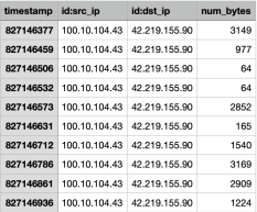
Figure 1: A very small subset of NetFlow data extracted from the UGR-16 dataset. This small subset is extracted to be used for the illustrative example of our encoding.

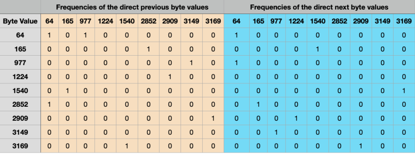
Figure 2: Frequencies of the direct previous/next bytes values for each of the unique byte values that are present in Figure 1.

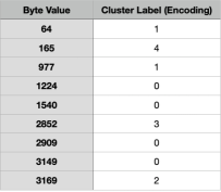
Figure 3: Cluster labels assigned to the unique byte values used in the example. The assigned cluster labels are used as the encoding for the unique byte values. In this example, we have used five clusters to cluster the vectors.

5.4 Implementation Details

As shown in our illustrative example, a vector is generated for each unique feature value $v$. As these vectors are clustered together using KMeans, the sizes of the vectors must have the same size. Furthermore, all vectors must store the same information (frequency values regarding a particular feature value) at the exact same position.

As shown in Figure 2, the first half of each vector (marked in brown) stores the frequencies of the direct previous values and the second half (marked in blue) stores the frequencies of the direct next values. Furthermore, the size of each vector is equal to twice the number of unique feature values. This is to make sure that each vector has the same structure and size. The structure in Figure 2 is a step in the right direction, but it does have limitations:

• It could create many sparse vectors.

• The size of each feature depends on the number of unique values for a given feature. If the number grows very large, then the size of the vectors would also grow very large.

• We cannot capture the behaviour in which a feature value $v$ occurs frequently with itself. We frequently observe in NetFlow data that the previous/next value of $v$ is itself, indicating repetitive software behaviour.

This last limitation is somewhat tricky. The counts of the value itself are somewhere in the table. For instance, for value 64 in Table 2 it is in the column labeled 64. The issue is that for different data rows, these self-contexts are in different columns. Thus rows with only self-contexts would receive a large distance. In our view, such repetitive behaviour is indicative of similar software and should not depend on the exact flow value.

We resolve this we add two columns to store the previous self-frequency and the next self-frequency. The self-frequency refers to the frequency in which $v$ has itself as its previous/next value. In addition to storing the self-frequency, we have also included an additional entry that stores the logarithm of the frequency of $v$ (marked in red). This way the frequency of $v$ also influences the distance computation between vectors. Furthermore, this entry helps to differentiate features that have similar previous/next values but different frequencies.

To resolve the first two limitations, we divide the space of the previous and next values into ten bins each using percentiles. This gives a vector of length 20 for each feature value $v$. In fact, this solution gives us control over the size of the vector by changing the number of bins that are used to divide the space of the previous/next values. Figure 4 presents the final generalised structure that is used in the implementation of our encoding.

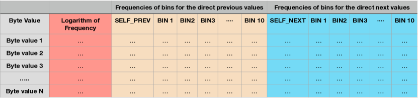
Figure 4: Generalised vector structure that is used for each unique feature value within our encoding algorithm.

Since KMeans chooses the initial centroids at random, each run of KMeans could lead to different final clusters. We therefore run KMeans ten times and take the best run to create our encoding for the unique feature values. We use the Silhouette Coefficient as our metric to evaluate how well the clusters were formed for the vectors that we have generated. To compute the Silhouette Coefficient, we use the python that is provided by scikit-learn [7]

Figure 5 provides a high-level overview of our data processing pipeline. For the clustering of the vectors, we have used the KMeans Clustering implementation that is provided by Scikit-learn machine-learning package [5]. We opted to use KMeans clustering to cluster the vectors as we can fix the number of clusters that can be created and thus we can fix the size of our encoding.

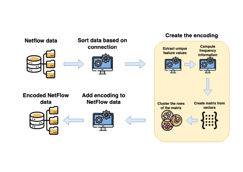
Figure 5: High-level overview of our data processing pipeline. The pipeline shows how the encoding is created for the given NetFlow input data using our encoding algorithm.

6 Evaluation of Our Encoding

In this section, we describe how we evaluate our encoding within the task of network anomaly detection. The goal of our evaluation is to show that machine learning algorithms can use our encoding to extract contextual information from NetFlow data and use it to learn more accurate models for network anomaly detection. To this aim, we train several machine learning models in an unsupervised manner to detect different network attacks. For each selected machine learning algorithm, we train two models; one that uses our encoding within the set of input features and one that does not use our encoding. The performance of the two models is then compared to each other. Specifically, we compare the performance of the models based on Balanced Accuracy and $F_{1}$ score

6.1 Machine Learning Models Selection

To evaluate the effectiveness of our encoding on learning (machine learning) models for network anomaly detection, we have selected popular machine learning methods for network anomaly detection.

State Machine Model

A state machine model, formerly known as finite state automaton, is a mathematical model to model sequential behaviour. These can be learned passively from data using state-merging algorithms. As state machines model sequential behaviour, they are well-suited to modelling NetFlow. We create fixed-size sequences from only benign NetFlow data and then use them to learn a state machine model. The model is then used to detect any sequential behaviour that deviates from the learned behaviour. For the learning of state machine models for our evaluation, we use Flexfringe [30] as this framework provides the ability to use different merging heuristics that can be used for the learning of a model.

Isolation Forest

Isolation forest is a well-known anomaly detection method. The idea is that using an ensemble of trees to find instances that have on average short path lengths within the trees [17]. Isolation forests detect point anomalies instead of sequential ones. We use the scikit-learn implementation of the isolation forest[6].

Local Outlier Factor (LOF)

Local outlier factor is another well-known anomaly detection method. The idea behind local outlier factor is that instances that are grouped in a dense neighbourhood are considered to be benign instances and instances in a neighbourhood with few other instances are considered anomalous instances. We use the scikit-learn implementation of local outlier factor [8]

Deep Neural Network - LSTM

In recent years, deep neural networks have been very popular to be used for anomaly detection. DeepLog is a well-known work that uses an LSTM to detect system anomalies from the log that are collected from the system [13]. The LSTM is used to model the sequential behaviours that can occur within the system. Similar to state machine models, only benign data is used for the learning of the model and the model is used to detect any sequential behaviours that deviate from what was learned from the training data. We use the PyTorch implementation of DeepLog [2].

6.2 Comparison Between Encoding Methods

To evaluate the effectiveness of our encoding, we have selected an existing encoding based on percentiles and a naive frequency-based encoding as baselines. The percentiles method divides the space of a given feature into $b$ number of bins. The encoding of a feature $v$ would be the bin that it falls into. The frequency method uses the frequency of the feature values to create an encoding; if a feature value $v$ has occurred at least $x$ number of times, then the raw feature values are used, otherwise it would be binned with other features values that did not meet the threshold $x$. This low frequency bin is subsequently divided into different bins using the percentiles method.

6.3 Dataset Selection

To evaluate our approach, we use three different datasets to learn models for anomaly detection. For the first dataset, we created a new dataset for our project [1]. This dataset (AssureMOSS) contains both benign and malicious NetFlows gathered from a Kubernetes cluster running multiple applications [11]. The architecture of the cluster is presented in Figure 6. For the generation of this dataset, 30 participants were asked to use the applications to generate benign NetFlow data. Furthermore, three different attack scenarios were constructed (DoS attack, lateral movement and malicious code deployment) using a threat matrix proposed by Microsoft [20]. The attack scenarios were launched by ourselves against the cluster, while the participants were using the applications.

For the second dataset, we selected a well-known data that is used by many works; the CTU-13 dataset [14]. This dataset contains both benign network traffic data that was generated by real users and malicious network traffic data generated by different malware. Thirteen captures were collected from different botnet samples.

For the third dataset, we selected the UGR-16 dataset [18]. This dataset contains a large volume of NetFlows collected from a Spanish ISP. The benign data were produced by real users and different types of attacks were launched to generate the malicious data.

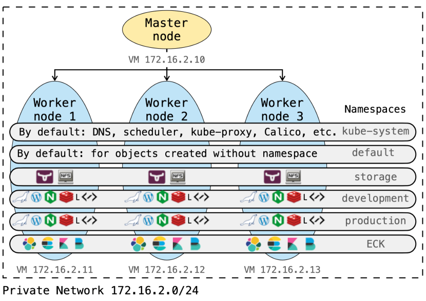
Figure 6: Architecture of the Kubernetes Cluster that was used to generate the ANONYMISED dataset

6.4 Feature Selection

For each dataset, we use the same features to pre-process the NetFlow data for training the machine learning models; the used protocol, the total number of bytes, the total number of packets, and the flow duration. Using only these four features, our encoding does not rely on operating system/network-specific features and can be used on different types of networks. We do not include source/destination ports as a feature for our encoding as these tend to be operating system/network specific. Furthermore, port information could sometimes be a spurious feature, i.e., a feature that is not indicative of the class but correlates with the class label.

We use the CTU-13 dataset to show how the source port is a spurious feature of the dataset. We believe that the source port feature from the CTU-13 dataset leaks information on the label of flow and it should not be blindly used to learn a model; the original authors of the dataset used virtual machines that were running Windows XP to generate the malicious flows of the malware. For this operating system, the default ephemeral ports start at 1025 and end at 5000 [4].

By plotting the distribution of the protocols for both benign and malicious data we can see a clear difference in the distributions of the source ports. Figure 7 shows the distribution of the source ports for the benign and malicious flows from all scenarios. Looking at the distribution of the source ports of the malicious data, a large portion of the flows seems to use a source port that is lower than 6000. The top three ports used in the malicious flows are 2077, 1025 and 2079. All these three port numbers fall within the range used by the virtual machines. Thus, by using the source port number the model does not try to learn whether it can distinguish malicious flows from benign flows but rather whether it can detect flows coming from a virtual machine. Thus, using the source port information to train the model would falsely lead to a better performance of the model and we therefore did not consider source/destination ports to be used a feature for our encoding.

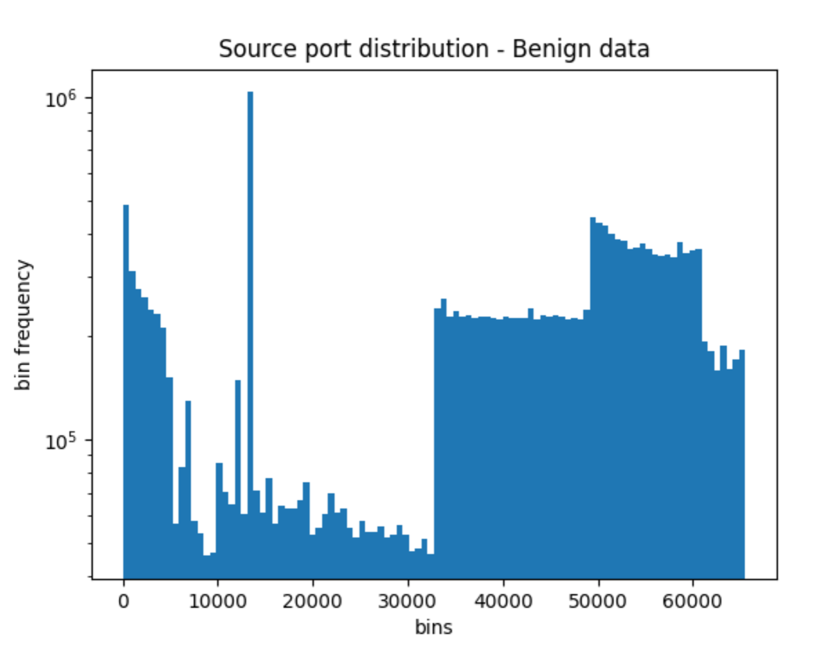
(a) Source port distribution of benign flows

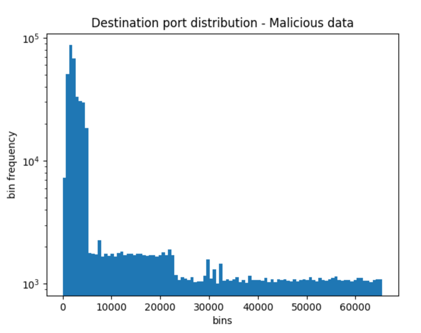
(b) Source port distribution of malicious flows

Figure 7: Source port distribution in the CTU-13 dataset.

6.5 Encoding Train & Test Data

As we perform anomaly detection in an unsupervised manner, we use only benign NetFlow data as training data for the machine learning models. The test data can contain both benign and malicious NetFlows. We now describe how we selected the train and test data for each dataset.

For the CTU-13 dataset, we have used the split that the authors of the dataset have proposed in [14] to create our train and test set. The train set contains about 720 thousand NetFlows and our test set contains about 522 thousand NetFlows.

For the UGR-16 dataset, we created our train set using benign data from the first week of each month in the calibration data and we create our test using both benign and malicious data from the first week of each month from the test data. The train set contains about 600 thousand NetFlows and the test set contains about 664 thousand.

For the dataset from our project, we selected the benign data from the first half-hour of data to create our training data and the remaining data is used to create the test data. The train set contains about 120 thousand NetFlows and the test set contains about 275 thousand.

Once the train and test set has been created for each dataset, they are concatenated together to create a larger set to be used as input for our encoding algorithm. Once the encoding has been created from this set, the encoding is added to the train and test set as extra columns.

6.6 Creating Sequences For Sequential Models

As we are using two machine learning models that learn the sequential behaviour from sequences, we need to transform the NetFlow data into sequences. Each sequence consists of a list of symbols. Each flow is transformed into a symbol and it is created by concatenating the encoding of the selected features together to form a single string with the following form: $PROTOCOL\_BYTES\_PACKETS\_DURATION$. Note that the protocol feature is already categorical, therefore we do not need to run our encoding algorithm on this feature. However, we did use an integer encoding that converts each protocol to a numerical value. For the creation of traces, we use a sliding window of length 20 on symbols from the same connection (i.e. combination of source and destination host). We drop traces that have a length smaller than the size of the sliding window.

7 Results

In this section, we empirically demonstrate the effectiveness of our encoding. Each selected NetFlow dataset is encoded using each encoding method and the encoded NetFlow data is used to train the selected machine learning models to detect network anomalies in an unsupervised manner. The effectiveness of our encoding is evaluated based on how well the machine learning models can detect anomalies using our encoding compared to baseline encodings. The performance results of the machine learning models are shown in Figures 8-16 and Table II. All performance results, with the exception of the DeepLog model (due to run-time), are average results over ten runs.

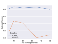
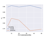
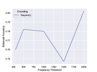
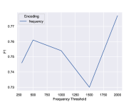
Figure 8: Performance results of state machines (for each encoding method) on detecting anomalies on the ANONYMISED dataset. The results that are presented in the figure is the average results of the model over 10 runs.

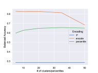
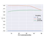
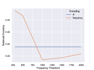
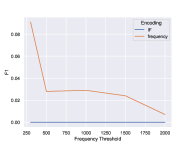
Figure 9: Performance results of isolation forest (for each encoding method) on detecting anomalies on the ANONYMISED dataset. The results that are presented in the figure is the average results of the model over 10 runs.

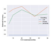
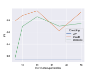
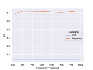
Figure 10: Performance results of local outlier factor (for each encoding method) on detecting anomalies on the ANONYMISED dataset.The results that are presented in the figure is the average results of the model over 10 runs.

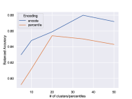
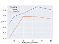
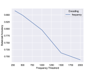
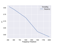
Figure 11: Performance results of state machines (for each encoding method) on detecting anomalies on the CTU-13 dataset. The results that are presented in the figure is the average results of the model over 10 runs.

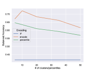
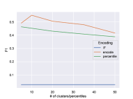
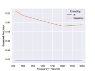
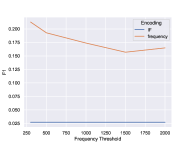
Figure 12: Performance results of isolation forest (for each encoding method) on detecting anomalies on the CTU-13 dataset. The results that are presented in the figure is the average results of the model over 10 runs.

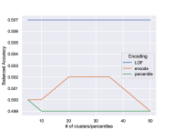
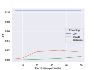
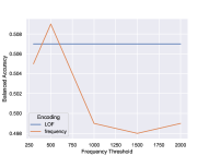
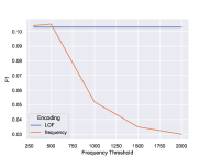
Figure 13: Performance results of local outlier factor (for each encoding method) on detecting anomalies on the CTU-13 dataset. The results that are presented in the figure is the average results of the model over 10 runs.

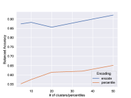
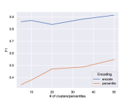
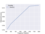
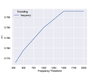
Figure 14: Performance results of state machines (for each encoding method) on detecting anomalies on the UGR-16 dataset. The results that are presented in the figure is the average results of the model over 10 runs.

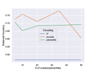
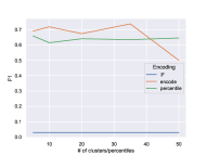
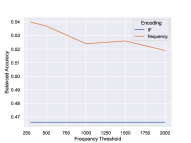
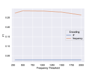
Figure 15: Performance results of isolation forest (for each encoding method) on detecting anomalies on the UGR-16 dataset. The results that are presented in the figure is the average results of the model over 10 runs.

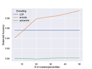
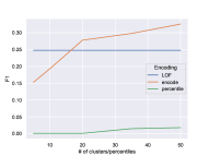
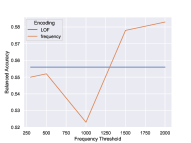
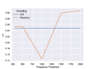
Figure 16: Performance results of local outlier factor (for each encoding method) on detecting anomalies on the UGR-16 dataset. The results that are presented in the figure is the average results of the model over 10 runs.

TABLE II: Partial performance results of DeepLog on ANONYMISED dataset. Performance results is computed over only one single run.

Encoding	Balanced Accuracy	$F_{1}$
ENCODE (5 clusters)	0.782	0.734
Percentile (5 bins)	0.482	0.332
Frequency (Threshold = 300)	-	-

7.1 Overall Results

Overall, when we look at the performance that are shown in Figures 8-16 and Table II, we see that the models achieve a significantly higher balanced accuracy and $F_{1}$ score when our encoding algorithm was used to encode the NetFlow data. This empirically demonstrates that the models can use the context that we define in our encoding to learn a better contextual correlation between the feature values of the NetFlow data and use it to better detect anomalies within the data.

Although it is a standard encoding method, the percentile encoding performs much worse than ours. We believe its low performance is due to flow similarity being based on the values themselves and that flows with similar values are not necessarily the same. Furthermore, it does not store any contextual information on how these values co-occur with each other.

Sequential machine learning models could in theory learn such behaviour, but even these perform much better using our method. Since we store some contextual information within each encoded value, even non-sequential machine learning methods can learn some sequential information using our encoding. You see this effect for the isolation forest detector, which performs much better using this information than using the raw feature values.

The low performance of the frequency encoding can be explained by the fact the encoding only stores information on the frequently occurring (based on a given threshold) features values within the data and the infrequent feature values are then binned together. Similar to the percentile encoding, this encoding does not store the context of how feature values co-occur with each other (for both the infrequent and frequent feature values).

When comparing the different machine learning methods, we see that LOF performs worse on the CTU-13 and UGR-16 datasets when our encoding or the percentile encoding is used. In fact, we obtain better results when the model is trained using simply the raw feature values. LOF treats the encoded values as integers and computes distances based on them. These distances are not that meaningful, explained the poor performance. LOF is also the only method for which it was better to encode the data using the frequency encoding (see Figure 13). The main reason for this is that we keep the raw values intact for high frequencies, making the distances somewhat meaningful. Still LOF performs much worse than the other methods that can use our encoding in a meaningful way.

Also the results obtained using DeepLog are promising, but only based on a single run (of one epoch) of the model on the AssureMOSS dataset. We only managed to get DeepLog working on the AssureMOSS dataset, and only for the case where we used 5 clusters in our encoding and 5 bins for the percentile encoding. We tested DeepLog both with and without GPU. For cases with a larger number of clusters or bins our machine ran out of memory. This can be caused by the number of unique symbols we introduce when we increase the size of the clusters/bins (more clusters or bins means that we have more symbols). Though the results do show that DeepLog achieves much better performance using our encoding, future work is needed to determine the significance.

7.2 The Effect of Cluster Number On Model Performance

A key parameter of our encoding is the number of clusters used. The larger this number, the more distinctions are made between flows, but at a cost of increased complexity. Based on the performance results that are shown in Figures 8-16, we see that the increase in the number of clusters can have different effects on the performance of the machine learning models; it can increase the performance of the model (see Figure 10, Figure 11 and Figure 14), it can decrease the performance of the model (see Figure 9, Figure 12 and Figure15), and it can also have no significant effect on the performance of the model (see 8. The increase in performance seems to be more common with state machine models and the decrease in performance seems to be more common with isolation forests. This shows it is important to tune this parameter when using our encoding.

8 Use-case and robustness

From our experimental result, we observe that state machines with 35 clusters perform best. To give some more insight into what these numbers mean, we display the output an analyst will see when running this anomaly detection system. The system produces log-likelihood values. In our experiments, we use a fixed decision threshold tuned on the training data to obtain counts on the false/true positives and negatives. When using the system in a real application, we believe it is actually better to simply display these loglikelihood values over time. Plots for this system on the CTU-13 data are shown in Figure 17.

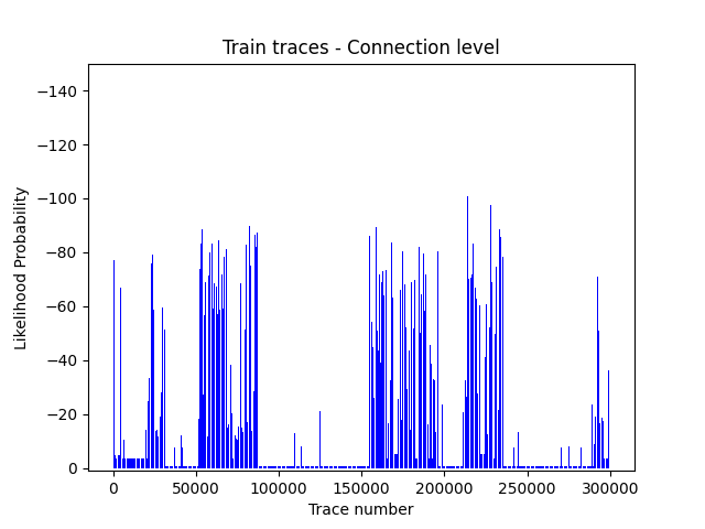
(a) Loglikelihood values for train data.

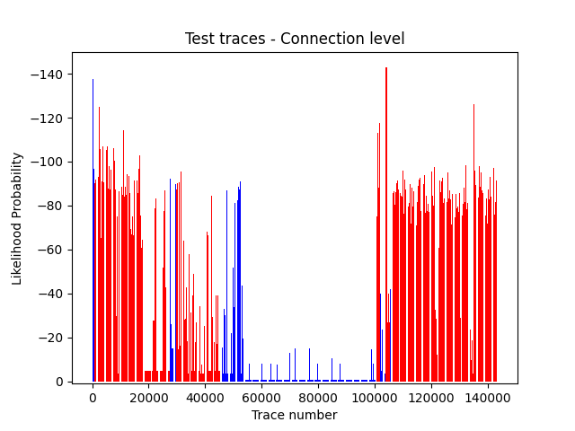
(b) Loglikelihood values for test data.

Figure 17: Outputs from the state machine method for CTU-13, blue=benign, red=malicious.

The loglikelihoods are plotted over time. An analyst can use this to quickly discover whether an attack is real or a false alarm. We frequently see multiple high (small) loglikelihood values when malicious traces occur. Also, we observe that anomalous flows exist in the train data, as simply some connections are infrequent. The loglikelihood values for the test data tend to be higher (smaller) when new infrequent flows occur. We can also clearly see from this figure that, although the performance values in our experiments are computed on a per flow basis, in practice it makes more sense to simply display these values. In fact, we could argue that the method only triggers a handful of false alarms by looking at how many blue peaks (grouped on timestamp) occur in the test data. Furthermore, we also clearly see that one attack creates many peaks in the loglikelihood scores while only one of these would be sufficient to trigger an investigation.

TABLE III: Performance results of state machine model when malicious data is perturbed

Amount of
Perturbation	Balanced Accuracy	$F_{1}$	Precision	Recall
Fixed 10	0.915	0.860	0.754	1.0
Random 50%	0.915	0.860	0.754	1.0
Random 80%	0.915	0.860	0.754	1.0
Without %	0.850	0.797	0.754	0.844

8.1 Experimental Results

To test the robustness, we display the performance of the state machine model after adding different amount of perturbation to the number of bytes and packets in Table III. We used three different perturbation for the malicious: add fixed value of to the two features, adding a random perturbation of 50% of the feature value and adding a random perturbation of 80% of the feature value. Adding the perturbation to the feature values would cause them to be put into the cluster in which all infrequent values (with low co-occurrences) are put. The performance of the state machine model increases when we add perturbation to the features. This shows that our encoding (with combination of a state machine model) is robust against an attacker that tries to randomly or structurally modify their network traffic to evade detection.

9 Conclusion & Future Work

We present a new encoding algorithm that pre-processes a NetFlow dataset for machine learning. The encoding algorithm uses the frequency of the feature values and the frequencies of co-occurrences between the feature values to compute a context in which the feature values occur. The context is then used to group feature values to create an encoding for the given feature. The intuition is that feature values that occur in similar contexts and are similarly frequent are indicative of similar software and should therefore receive the same encoding label.

We empirically demonstrate the effectiveness of our encoding by using it to encode NetFlow data from three different datasets and using the encoded data to learn four different machine models to detect network anomalies in an unsupervised manner. For each dataset, we computed the performance results of the machine learning models and compared them to the performance results achieved using two other encoding methods. Based on the empirical results, the machine learning models achieved much better performance using our encoding.

A method base on state machines to model the sequential behavior in NetFlows works best in our experiments. For this method we present a use-case that demonstrates the type of information an analyst receives form the system and how to use it. Additionally, we demonstrate that this method is resilient against possible perturbations made by attackers aiming to avoid detection. In fact, such perturbations only make the data more anomalous, leading to an increase in detection rates.

For this work, we have only used NetFlow for our encoding. For future work on our encoding algorithm, we would like to evaluate it on other types of data e.g. software log data. We believe that our encoding could also be beneficial for encoding software log data and it would also be interesting to investigate the effectiveness of our encoding algorithm on other types of data.

It would also be interesting to evaluate our encoding algorithm on more types of machine learning models. For instance, although it is not our main goal, we believe that the encoding is also useful in supervised machine learning.

Finally, we are working on a streaming version of our encoding that can be run in real-time in NetFlow collectors.

References

- [1] AssureMOSS.
- [2] DeepLog - PyTorch implementation of Deeplog: Anomaly detection and diagnosis from system logs through deep learning. https://github.com/Thijsvanede/DeepLog.
- [3] ENCODE: Encoding NetFlows for Network Anomaly Detection. https://github.com/tudelft-cda-lab/ENCODE.
- [4] Service overview and network port requirements - Windows Server — Microsoft Docs. https://docs.microsoft.com/en-us/troubleshoot/windows-server/networking/service-overview-and-network-port-requirements.
- [5] sklearn.cluster.KMeans — scikit-learn 1.1.1 documentation. https://scikitlearn.org/stable/modules/generated/sklearn.cluster.KMeans.html.
-
[6]
sklearn.ensemble.IsolationForest — scikit-learn 1.1.2 documentation.
https://scikit-learn.org/stable/modules/generated/sklearn.ensemble.
IsolationForest.html. - [7] sklearn.metrics.silhouette_score — scikit-learn 1.1.2 documentation. https://scikit-learn.org/stable/modules/generated/sklearn.metrics.silhouette_score.html.
- [8] sklearn.neighbors.LocalOutlierFactor — scikit-learn 1.1.2 documentation.
- [9] Abdulghani Ali Ahmed, Waheb A. Jabbar, Ali Safaa Sadiq, and Hiran Patel. Deep learning-based classification model for botnet attack detection. Journal of Ambient Intelligence and Humanized Computing, 1:1–10, mar 2020.
- [10] Jose Camacho, Gabriel Macia-Fernandez, Noemi Marta Fuentes-Garcia, and Edoardo Saccenti. Semi-supervised multivariate statistical network monitoring for learning security threats. IEEE Transactions on Information Forensics and Security, 14(8):2179–2189, aug 2019.
- [11] Clinton Cao and Agathe Blaise. AssureMOSS Kubernetes Run-time Monitoring Dataset, 2022.
- [12] Cisco Systems. Cisco IOS NetFlow - Cisco. https://www.cisco.com/c/en/us/products/ios-nx-os-software/ios-netflow/index.html, 2018.
- [13] Min Du, Feifei Li, Guineng Zheng, and Vivek Srikumar. Deeplog: Anomaly detection and diagnosis from system logs through deep learning. In Proceedings of the 2017 ACM SIGSAC conference on computer and communications security, pages 1285–1298, 2017.
- [14] S. Garcia, M. Grill, J. Stiborek, and A. Zunino. An empirical comparison of botnet detection methods. Computers & Security, 45:100–123, sep 2014.
- [15] Mohammad Hashem Haghighat and Jun Li. Intrusion detection system using voting-based neural network. Tsinghua Science and Technology, 26(4):484–495, aug 2021.
- [16] Xavier Larriva-Novo, Mario Vega-Barbas, Víctor A. Villagrá, Diego Rivera, Manuel Álvarez-Campana, and Julio Berrocal. Efficient Distributed Preprocessing Model for Machine Learning-Based Anomaly Detection over Large-Scale Cybersecurity Datasets. Applied Sciences 2020, Vol. 10, Page 3430, 10(10):3430, may 2020.
- [17] Fei Tony Liu, Kai Ming Ting, and Zhi-Hua Zhou. Isolation forest. In 2008 Eighth IEEE International Conference on Data Mining, pages 413–422, 2008.
- [18] Gabriel Maciá-Fernández, José Camacho, Roberto Magán-Carrión, Pedro García-Teodoro, and Roberto Therón. UGR‘16: A new dataset for the evaluation of cyclostationarity-based network IDSs. Computers and Security, 73:411–424, mar 2018.
- [19] Roberto Magán-Carrión, Daniel Urda, Ignacio Díaz-Cano, and Bernabé Dorronsoro. Towards a Reliable Comparison and Evaluation of Network Intrusion Detection Systems Based on Machine Learning Approaches. Applied Sciences 2020, Vol. 10, Page 1775, 10(5):1775, mar 2020.
- [20] Microsoft. Threat matrix for Kubernetes. https://www.microsoft.com/security/blog/2020/04/02/attack-matrix-kubernetes/, 2020.
- [21] Tomas Mikolov, Kai Chen, Greg Corrado, and Jeffrey Dean. Efficient estimation of word representations in vector space. In 1st International Conference on Learning Representations, ICLR 2013 - Workshop Track Proceedings. International Conference on Learning Representations, ICLR, jan 2013.
- [22] Nour Moustafa and Jill Slay. UNSW-NB15: A comprehensive data set for network intrusion detection systems (UNSW-NB15 network data set). 2015 Military Communications and Information Systems Conference, MilCIS 2015 - Proceedings, dec 2015.
- [23] Quoc Phong Nguyen, Kar Wai Lim, Dinil Mon Divakaran, Kian Hsiang Low, and Mun Choon Chan. GEE: A Gradient-based Explainable Variational Autoencoder for Network Anomaly Detection. 2019 IEEE Conference on Communications and Network Security, CNS 2019, pages 91–99, jun 2019.
- [24] Beny Nugraha, Anshitha Nambiar, and Thomas Bauschert. Performance Evaluation of Botnet Detection using Deep Learning Techniques. Proceedings of the 11th International Conference on Network of the Future, NoF 2020, pages 141–149, oct 2020.
- [25] University of New Brunswick. Datasets — Research — Canadian Institute for Cybersecurity — UNB. https://www.unb.ca/cic/datasets/index.html.
- [26] Gaetano Pellegrino, Qin Lin, Christian Hammerschmidt, and Sicco Verwer. Learning behavioral fingerprints from Netflows using Timed Automata. In Proceedings of the IM 2017 - 2017 IFIP/IEEE International Symposium on Integrated Network and Service Management, pages 308–316. Institute of Electrical and Electronics Engineers Inc., jul 2017.
- [27] Michal Piskozub, Riccardo Spolaor, and Ivan Martinovic. MalAlert: Detecting malware in large-scale network traffic using statistical features. In Performance Evaluation Review, volume 46, pages 151–154, 2019.
- [28] Shahab Shamshirband and Anthony T. Chronopoulos. A new malware detection system using a high performance-elm method. ACM International Conference Proceeding Series, jun 2019.
- [29] Duygu Sinanc Terzi, Ramazan Terzi, and Seref Sagiroglu. Big data analytics for network anomaly detection from netflow data. In 2nd International Conference on Computer Science and Engineering, UBMK 2017, pages 592–597. Institute of Electrical and Electronics Engineers Inc., oct 2017.
- [30] Sicco Verwer and Christian A. Hammerschmidt. Flexfringe: A passive automaton learning package. In Proceedings - 2017 IEEE International Conference on Software Maintenance and Evolution, ICSME 2017, pages 638–642, 2017.
- [31] Ibrahim Yilmaz and Rahat Masum. Expansion of Cyber Attack Data From Unbalanced Datasets Using Generative Techniques. 2019.
- [32] Tommaso Zoppi, Andrea Ceccarelli, Tommaso Capecchi, and Andrea Bondavalli. Unsupervised anomaly detectors to detect intrusions in the current threat landscape. ACM/IMS Trans. Data Sci., 2(2), apr 2021.
- [33] Tommaso Zoppi, Mohamad Gharib, Muhammad Atif, and Andrea Bondavalli. Meta-learning to improve unsupervised intrusion detection in cyber-physical systems. ACM Transactions on Cyber-Physical Systems, 5(4), sep 2021.