Reinforced Lin-Kernighan-Helsgaun Algorithms for the Traveling Salesman Problems

Abstract

TSP is a classical NP-hard combinatorial optimization problem with many practical variants. LKH is one of the state-of-the-art local search algorithms for the TSP. LKH-3 is a powerful extension of LKH that can solve many TSP variants. Both LKH and LKH-3 associate a candidate set to each city to improve the efficiency, and have two different methods, $\alpha$-measure and POPMUSIC, to decide the candidate sets. In this work, we first propose a Variable Strategy Reinforced LKH (VSR-LKH) algorithm, which incorporates three reinforcement learning methods (Q-learning, Sarsa, Monte Carlo) with LKH, for the TSP. We further propose a new algorithm called VSR-LKH-3 that combines the variable strategy reinforcement learning method with LKH-3 for typical TSP variants, including the TSP with time windows (TSPTW) and Colored TSP (CTSP). The proposed algorithms replace the inflexible traversal operations in LKH and LKH-3 and let the algorithms learn to make a choice at each search step by reinforcement learning. Both LKH and LKH-3, with either $\alpha$-measure or POPMUSIC, can be significantly improved by our methods. Extensive experiments on 236 widely-used TSP benchmarks with up to 85,900 cities demonstrate the excellent performance of VSR-LKH. VSR-LKH-3 also significantly outperforms the state-of-the-art heuristics for TSPTW and CTSP.

1 Introduction

Given a set of cities with certain locations, the Traveling Salesman Problem (TSP) is to find the shortest Hamiltonian route, along which a salesman travels from a city (depot) to visit all the cities exactly once and finally returns to the depot. The TSP and its variant problems, such as the TSP with time windows (TSPTW) [1, 2] and the colored TSP (CTSP) [3, 4], are all challenging combinatorial optimization problems. Algorithms designed for the TSP and its variant problems have many possible applications, such as the Vehicle Routing Problem (VRP) [5], collision-free scheduling of multi-bridge machining systems [6], rice harvesting schedules [7], etc.

Numerous approaches have been proposed for solving the TSP and its variant problems. Typical methods mainly include exact algorithms, approximation algorithms, and heuristic algorithms. Exact algorithms may be prohibitive for large-scale instances and approximation algorithms may suffer from weak optimality guarantees or empirical performance [8]. Heuristics are known to be the most efficient and effective approaches for solving the TSPs.

Since the Lin-Kernighan (LK) heuristic [9] was proposed, the LK-based algorithms [9, 10, 11, 12] have become one of the most popular series of local search heuristics for the TSP. Among them, the Lin-Kernighan-Helsgaun (LKH) algorithm [11, 12] is the most famous and also one of the state-of-the-art local search algorithms for the TSP. LKH optimizes the solutions by the $k$-opt method [13], which explores the solution space by replacing $k$ edges of the current tour. To reduce the search scope and improve the efficiency, LKH defines the candidate edges as LK does and restricts that the edges to be added during the $k$-opt process must be selected from the candidate edges. LKH associates a candidate set for each city, where it records several other candidate cities. The candidate edges in LKH consist of the edges between each city and its candidate cities.

In LK, the candidate set of each city records several other nearest cities. The earliest version of LKH [11] proposes an $\alpha$-measure method to determine the candidate sets, which uses an $\alpha$-value defined based on the minimum spanning tree [14] as a metric for evaluating the quality of the edges. The $\alpha$-measure further improves the performance of the $\alpha$-value by adding a $\pi$-value as penalties to each city. We denote the $\alpha$-value obtained after adding $\pi$-values as $\alpha^{\pi}$-value for clarity. Due to the better performance of the $\alpha^{\pi}$-value than the distance in determining the candidate cities, LKH [11] significantly improves the LK heuristic.

Recently, Taillard and Helsgaun [12] propose to apply the Partial OPtimization Metaheuristic Under Special Intensification Conditions (POPMUSIC) method to help LKH select the candidate edges. POPMUSIC is an efficient approach that can quickly generate high-quality solutions. Its main idea is to divide a solution into multiple sub-paths, and improve each sub-paths independently. LKH with the POPMUSIC method [12] first uses POPMUSIC to generate multiple tours, and then determines the candidate edges by merging all the edges that appeared in these tours. This approach can obtain the candidate sets within a shorter time than the $\alpha$-measure method [11], simultaneously guaranteeing the quality of the candidate sets. After determining the candidate sets by POPMUSIC, the order of the candidate cities is sorted according to the $\alpha$-value.

LKH-3 [15] is an extension of LKH that can be used to solve about 40 different TSP variants. LKH-3 solves these problems by transforming them into the constrained TSP [16, 17, 18], and uses the $k$-opt method to explore the solution space. LKH-3 allows searching in the infeasible solution space, and defines different violation functions for different problems to evaluate the violation extent of the given constraints. A solution is improved by $k$-opt in LKH-3 when the violation function is reduced, or the violation function is unchanged meanwhile the optimization objective is reduced. A route with zero violation values is feasible. The candidate sets in LKH-3 can also be selected by both $\alpha$-measure and POPMUSIC.

Both LKH and LKH-3 are successful and effective algorithms. However, the constant $\alpha^{\pi}$-value or $\alpha$-value may not be the best metric to determine or order the candidate cities, although they are well designed. During the $k$-opt process, both LKH and LKH-3 traverse the candidate sets in ascending order of the $\alpha^{\pi}$-value (or $\alpha$-value) to select the edges to be added. Such a traversal mechanism is inflexible and may limit the potential of the algorithms to find better solutions. In this work, we address the challenge of improving LKH and LKH-3, and introduce an effective method to combine reinforcement learning [19, 20, 21] with the LKH and LKH-3 algorithms. The proposed algorithms could learn to adjust the candidate sets adaptively and learn to choose appropriate edges to be added during the $k$-opt process by means of reinforcement learning methods.

Specifically, we first propose a Variable Strategy Reinforced LKH (VSR-LKH) algorithm, that combines three reinforcement learning methods, Q-learning, Sarsa, and Monte Carlo [19], with LKH to solve the TSP. The reinforcement learning is combined with the core $k$-opt process in LKH. VSR-LKH actually learns an adaptive Q-value to replace the $\alpha^{\pi}$-value (or $\alpha$-value) as the metric for evaluating the quality of the edges. Moreover, the variable strategy reinforcement learning method inspired from Variable Neighborhood Search (VNS) [22] could make use of the complementary of the above three reinforcement learning methods in reinforcing LKH (for example, some TSP instances can be solved well by Q-learning, but not by Sarsa, and vice versa). We then combine the variable strategy reinforcement learning method with LKH-3 to solve two typical variants of the TSP, TSPTW and CTSP. The resulting algorithm is denoted as VSR-LKH-3.

This paper is an extended and improved version of our conference paper [23], in which we proposed the VSR-LKH algorithm for the standard TSP and compared with LKH with the $\alpha$-measure method. In this paper, we make a more comprehensive empirical analysis of the VSR-LKH for the TSP, and further propose a new algorithm called VSR-LKH-3 that can handle various TSP variants. Due to the properties of the violation functions in LKH-3, we design a new reward function in the reinforcement learning framework of VSR-LKH-3 that considers both tour lengths and violation values. We do a more comprehensive comparison with LKH and LKH-3 with both the $\alpha$-measure and the POPMUSIC methods. We further compare VSR-LKH with the state-of-the-art (deep) learning based algorithm for the TSP, NeuroLKH [24], and compare VSR-LKH-3 with the state-of-the-art heuristic algorithms for the TSPTW [1, 2] and CTSP [4].

The principal contributions of this work are as follows:

• We propose to combine reinforcement learning with the effective LKH and LKH-3 algorithms to solve the TSP and its variants. Both LKH and LKH-3, with either the $\alpha$-measure or the POPMUSIC method can be significantly improved by our methods.

• VSR-LKH also significantly outperforms the state-of-the-art (deep) learning based algorithm for the TSP, NeuroLKH. Moreover, VSR-LKH-3 significantly outperforms the state-of-the-art heuristics for solving the TSPTW and CTSP. In particular, our method can help LKH-3 outperform the best-performing CTSP heuristic, providing 12 new best solutions among 65 public CTSP instances.

• We define a Q-value to replace the $\alpha^{\pi}$-value (or $\alpha$-value) used in LKH and LKH-3 for selecting and sorting the candidate cities. The Q-value can be adjusted adaptively by learning from the information of the solutions generated during the iterative search.

• Since heuristics for NP-hard combinatorial optimization problems usually need to search in the solution space, our approach suggests a method to improve heuristics by combining reinforcement learning with the core local search process.

The rest of this paper is organized as follows. Section 2 introduces basic concepts for the TSP, TSPTW, and CTSP. Section 3 presents related works of effective heuristics and (reinforcement) learning based methods in solving the TSPs, and further discusses the advantages of our proposed reinforcement learning method. Section 4 briefly introduces the existing LKH and LKH-3 algorithms. Sections 5 and 6 describes our proposed VSR-LKH and VSR-LKH-3 algorithms. Section 7 presents experimental results and analyses. Section 8 contains the concluding remarks.

2 Problem Definition

This section presents the definition of the problems to be addressed, TSP, TSPTW, and CTSP, respectively.

2.1 Traveling Salesman Problem

Given a complete, undirected graph $G=(V,E)$, where $V=\{1,2,...,n\}$ denotes the set of the cities and $E$ the set of all pairwise edges $\{(i,j)|i,j\in V\}$. Each edge $(i,j)\in E$ has a cost $d(i,j)$, e.g., the distance of traveling from city $i$ to city $j$. The TSP is to find a Hamiltonian route represented by a permutation $(c_{1},c_{2},...,c_{n})$ of cities $\{1,2,...,n\}$ that minimizes the total cost, i.e., $d(c_{1},c_{2})+d(c_{2},c_{3})+...+d(c_{n},c_{1})$, where $c_{1}=1$ is the depot.

2.2 Traveling Salesman Problem with Time Windows

In the TSP with Time Windows (TSPTW), each city $i\in{V}$ has a time window $[a_{i},b_{i}]$ that restricts the salesman from reaching city $i$ within the time window, and a service time $st_{i}$ that indicates the time length the salesman must stay in city $i$. In addition, we assume that waiting is permitted. If the salesman reaches city $i$ before $a_{i}$, he will wait until time $a_{i}$ to start the service. The TSPTW is to find the shortest Hamiltonian route on the graph $G=(V,E)$ while satisfying the time window constraints.

2.3 Colored Traveling Salesman Problem

In the Colored TSP (CTSP), the city set $V$ is divided into $m+1$ disjoint sets: $m$ exclusive city sets $Ec_{1},Ec_{2},...,Ec_{m}$ and one shared city set $Sc$. The cities of each exclusive set $Ec_{k}(k=1,2,...,m)$ must be visited by salesman $k$ and each city from the shared city set $Sc$ can be visited by any of the $m$ salesmen. City 1 (the depot) belongs to the shared set $Sc$ and is visited by all the salesmen. The CTSP needs to determine $m$ routes on the graph $G=(V,E)$ for the $m$ salesmen. Route $k$ ($k\in\{1,2,...,m\}$) can be represented by sequence ($c_{1}^{k},c_{2}^{k},...c_{l_{k}}^{k}$), where $c_{1}^{k}=1$ is the depot, $l_{k}$ is the number of cities in route $k$. The $m$ routes should satisfy the following constraints. First, each city except the depot can be visited exactly once, i.e., $\cup_{k=1}^{m}{\cup_{i=2}^{l_{k}}{\{c_{i}^{k}\}}}=V\backslash\{1\}$ and $\sum\nolimits_{k=1}^{m}{(l_{k}-1)}=|V\backslash\{1\}|$. Second, the cities belonging to exclusive set $Ec_{k}$ should be contained in sequence ($c_{1}^{k},c_{2}^{k},...c_{l_{k}}^{k}$), i.e., $\cup_{i=1}^{l_{k}}{c_{i}^{k}}\cap{Ec_{k}}=Ec_{k}$. The goal of the CTSP is to find $m$ routes with the minimum total cost, i.e., $\sum\nolimits_{k=1}^{m}{d(c_{1}^{k},c_{2}^{k})+d(c_{2}^{k},c_{3}^{k})+...+d(c_{l_{k}}^{k},c_{1}^{k})}$.

3 Related Work

This section reviews related works of effective heuristic algorithms and (reinforcement) learning based methods in solving the TSP, TSPTW, and CTSP.

3.1 Heuristic Algorithms

The LK series of algorithms [9, 10, 11, 12] introduced in Section 1 are a kind of state-of-the-art heuristics for the TSP based on local search. Additionally, the edge assembly crossover genetic algorithm (EAX-GA) [25, 26] is another kind of state-of-the-art TSP heuristics based on the genetic algorithms. EAX-GA is very efficient in solving TSP instances with tens of thousands of cities. However, it is hard to scale to super large instances, such as TSP instances with millions of cities, since the convergence of the population is too time-consuming and the memory required for storing the information of the population is huge. As an efficient local search algorithm, LKH can yield near-optimal solutions faster as compared with EAX-GA. Moreover, LKH is suitable for TSP instances with various scales, especially for super large instances, providing the best-known solution of the famous World TSP instance with 1,904,711 cities. This paper mainly focuses on improving the LKH and LKH-3 local search algorithms by reinforcement learning.

Effective heuristics for the TSPTW include the compressed-annealing heuristic [27], the general variable neighborhood search (GVNS) algorithm [1], and the variable iterated greedy variable neighborhood search (VIG_VNS) algorithm [2]. The compressed-annealing heuristic augments the temperature from traditional simulated annealing with the concept of pressure, and proposes a variable penalty function and stochastic search to allow the algorithm to search in infeasible solution space. The GVNS algorithm consists of a construction phase and an optimization phase. During the optimization phase, GVNS uses the variable neighborhood descend algorithm to improve the initial solution generated in the construction phase. The VIG_VNS algorithm proposes a destruction and construction procedure based on iterative greedy algorithms to explore the solution space and find better solutions.

The CTSP was first proposed in 2015 [3], where the authors presented a genetic algorithm with dual-chromosome coding to solve the problem. Subsequently, some population-based heuristics [28, 29] and a variable neighborhood search method [30] were proposed. More recently, He et al. proposed an effective iterated two-phase local search algorithm [31] and a grouping memetic algorithm (GMA) [4] that combines the EAX [26] crossover method with local search approaches. Among these heuristics, the GMA algorithm based on the EAX crossover method significantly outperforms the others.

3.2 Learning based Methods

Since there are few (reinforcement) learning based methods for the TSPTW and CTSP as compared to those for the TSP, this subsection mainly introduces the (reinforcement) learning based methods for the TSP.

(Reinforcement) learning based methods for the TSP can be divided into two categories. The first category solves the problems in an end-to-end manner. Algorithms belonging to this category are usually based on deep neural networks. When receiving an input instance, they use the trained learning model to generate a solution directly. For example, Bello et al. [32] address TSP by using the actor-critic method to train a pointer network. The S2V-DQN algorithm [8] applies reinforcement learning to train a graph neural network so as to solve several combinatorial optimization problems including the TSP. Goh et al. [33] use an encoder based on a standard multi-headed transformer architecture and a Softmax or Sinkhorn [34] decoder to directly solve the TSP. There are also some algorithms based on deep reinforcement learning for variants of the TSPTW [35, 36]. These methods provide good innovations in the field of applying machine learning to solve combinatorial optimization problems. They can yield near-optimal or optimal solutions for small TSP instances with less than hundreds of cities. However, they are usually hard to scale to large instances (with more than thousands of cities) due to the complexity of deep neural networks.

Methods belonging to the second category combine (reinforcement) learning methods with traditional algorithms. Some of them use traditional algorithms as the core and frequently call the learning models to make decisions. For example, Liu and Zeng [37] employ reinforcement learning to construct mutation individuals in the previous version of EAX-GA [25] and report better results than EAX-GA and LKH on instances with up to 2,392 cities. But the efficiency of their proposed algorithm is not as good as that of LKH. Costa et al. [38] and Sui et al. [39] use deep reinforcement learning to guide 2-opt and 3-opt local search operators, and report results on instances with no more than 500 cities. Other methods separate the learning models and traditional algorithms. They first apply learning models to yield initial solutions [40] or some configuration information [24], and then use traditional algorithms to find high-quality solutions followed the obtained initial solutions or information. Among them, the NeuroLKH algorithm [24] is one of the state-of-the-art, which uses a Sparse Graph Network with supervised learning to generate the candidate edges for LKH. It reports better or similar results compared with LKH in instances with less than 6,000 cities. However, the supervised learning method makes its performance depend much on the structure of the training instances, the generated fixed candidate edges may limit its flexibility and robustness, and the complexity of the networks requires huge resources for large instances (such as instances with tens of thousands cities).

In summary, (reinforcement) learning based methods with deep neural networks for the TSP may suffer from the bottleneck of hardly solving large scale instances, and the combination of traditional reinforcement learning methods (training tables, not deep neural networks) with existing (heuristic) algorithms may reduce the algorithm efficiency. Our proposed reinforcement learning method can avoid these issues. On the one hand, instead of using deep neural networks, our reinforcement learning method uses the traditional reinforcement algorithms including Q-learning, Sarsa, and Monte Carlo [19] to train a table that stores the adaptive Q-value to guide the search directions during the $k$-opt process. On the other hand, we combine reinforcement learning with the core search steps of LKH and LKH-3 in a reasonable way, that can adjust the candidate sets adaptively. Therefore, our proposed algorithms can solve very large instances efficiently and effectively, such as the TSP instance with 85,900 cities and CTSP instances with 7,397 cities used in our experiments.

4 Revisiting the LKH and LKH-3 Algorithms

This section first introduces the LKH algorithm, and then introduces the extended implementation of LKH-3 over LKH. Our proposed VSR-LKH and VSR-LKH-3 algorithms are implemented based on them.

4.1 The LKH algorithm

The main framework of LKH is simple. In each iteration, LKH first generates an initial solution, and then uses the $k$-opt method [13] to improve the solution to a local optimum. The edges to be added during the $k$-opt process in LKH are restricted by the candidate sets. This subsection introduces the core approaches used in LKH, including the $k$-opt process and the methods for constructing the candidate sets, i.e., $\alpha$-measure and POPMUSIC.

4.1.1 The $k$-opt Process in LKH

The $k$-opt method tries to improve the current solution by replacing $k$ edges in the current TSP tour with $k$ new edges. The key point of $k$-opt is how to select the edges to be removed $\{x_{1},...,x_{k}\}$ and the edges to be added $\{y_{1},...,y_{k}\}$. In LKH, the edges involved in a $k$-opt move are connected. Thus selecting the edges can be regarded as selecting a sequence (cycle) of cities, i.e., $(\mathbf{p}_{1},\mathbf{p}_{2},...,\mathbf{p}_{2k},\mathbf{p}_{2k+1})$ as depicted in Figure 1, where $(\mathbf{p}_{2i-1},\mathbf{p}_{2i})=x_{i}$, $(\mathbf{p}_{2i},\mathbf{p}_{2i+1})=y_{i}$ ($i\in\{1,...,k\}$), and $\mathbf{p}_{2k+1}=\mathbf{p}_{1}$.

The $k$-opt process in LKH is actually a partial depth-first search process, that the maximum depth of the search tree is restricted to $k_{max}$, i.e., $k$-opt can replace at most $k_{max}$ (5 by default in LKH) edges in the current tour. Specifically, $k$-opt starts from a starting city $\mathbf{p}_{1}$ (i.e., root of the search tree), then alternatively selects an edge to be removed, i.e., edge $(\mathbf{p}_{2i-1},\mathbf{p}_{2i})$, and an edge to be added, i.e., edge $(\mathbf{p}_{2i},\mathbf{p}_{2i+1})$, until the entire search tree is traversed or a $k$-opt move that can improve the current tour is found. The selection of the cities $\mathbf{p}_{2i}$ and $\mathbf{p}_{2i+1}$ should satisfy the following constraints:

• C-I: for $i\geq 2$, connecting $\mathbf{p}_{2i}$ back to $\mathbf{p}_{1}$ should result in a feasible TSP tour.

• C-II: $\mathbf{p}_{2i+1}$ is always chosen so that $\sum\nolimits_{j=1}^{i}(d(\mathbf{p}_{2j-1},\mathbf{p}_{2j})-d(\mathbf{p}_{2j},\mathbf{p}_{2j+1}))>0$.

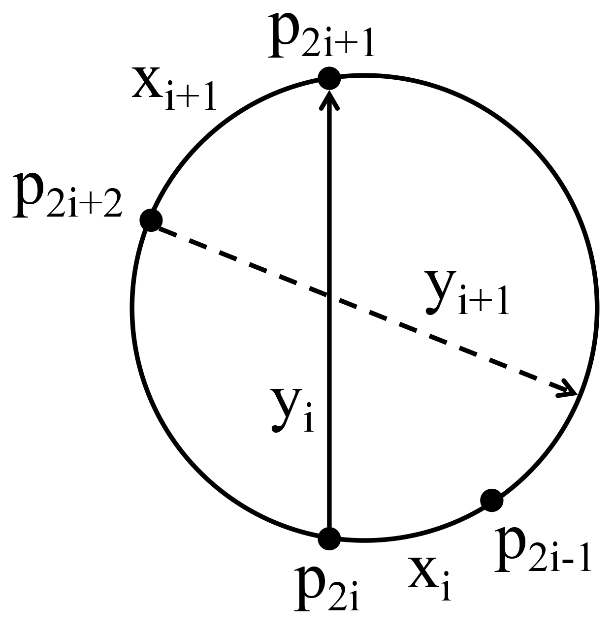
Figure 1: Regarding edges involved in $k$-opt as a sequence of cities.

Input: input solution: $S_{in}$, starting city: $\mathbf{p}_{1}$, sequence of the involved cities: $\mathbf{p}$, current search depth: $i$, the maximum search depth: $k_{max}$

Output: output solution $S_{out}$, sequence of the involved cities $\mathbf{p}$

1 for $h\leftarrow 1:2$ do

2       $\mathbf{p}_{2i}\leftarrow\mathbf{p}_{2i-1}^{h}$;

3       if $\mathbf{p}_{2i}$ does not satisfy the constraint C-I then

4            continue;

5            

6      if $i\geq 2\wedge\sum_{j=1}^{i}{d(\mathbf{p}_{2j-1},\mathbf{p}_{2j})}<\sum_{j=1}^{i-1}{d(\mathbf{p}_{2j},\mathbf{p}_{2j+1})}+d(\mathbf{p}_{2i},\mathbf{p}_{1})$ then

7             $S_{out}\leftarrow S_{in}$;

8             for $j\leftarrow 1:i$ do

9                  remove edge $(\mathbf{p}_{2j-1},\mathbf{p}_{2j})$ from $S_{out}$;

10            for $j\leftarrow 1:i-1$ do

11                  add edge $(\mathbf{p}_{2j},\mathbf{p}_{2j+1})$ into $S_{out}$;

12            Add edge $(\mathbf{p}_{2i},\mathbf{p}_{1})$ into $S_{out}$;

13             return $(S_{out},\mathbf{p})$;

14            

15      if $i=k_{max}$ then return $(S_{in},\emptyset)$;

16       for $j\leftarrow 1:5$ do

17             $\mathbf{p}_{2i+1}\leftarrow$ the $j$-th city in $CS^{\mathbf{p}_{2i}}$;

18             if $\mathbf{p}_{2i+1}$ doesn’t satisfy constraint C-II then

19                  continue;

20                  

21            $(S_{temp},\mathbf{p^{\prime}})\leftarrow k$-opt($S_{in},\mathbf{p}_{1},\mathbf{p}\cup\{\mathbf{p}_{2i},\mathbf{p}_{2i+1}\},i+1,k_{max}$);

22             if $l(S_{temp})<l(S_{in})$ then

23                  return $(S_{temp},\mathbf{p^{\prime}})$;

24            

25      

26return $(S_{in},\emptyset)$;

Algorithm 1 $k$-opt($S_{in},\mathbf{p}_{1},\mathbf{p},i,k_{max}$)

Let $c^{1}$ be a city randomly picked from the two cities connected with city $c$ in the current TSP tour, $c^{2}$ be the other, $l(S)$ be the length of solution $S$, $CS^{c}$ be the candidate set of city $c$. The procedure of the $k$-opt process is presented in Algorithm 1. As shown in Algorithm 1, the $k$-opt process tries to improve the current solution by traversing the partial depth-first search tree from the root $\mathbf{p}_{1}$. When selecting the edge to be removed, i.e., edge $(\mathbf{p}_{2i-1},\mathbf{p}_{2i})$ (the same as selecting $\mathbf{p}_{2i}$ from $\mathbf{p}_{2i-1}$), the algorithm traverses the two cities connected with city $\mathbf{p}_{2i-1}$ in the current TSP tour (lines 1-2). When selecting the edge to be added, i.e., edge $(\mathbf{p}_{2i},\mathbf{p}_{2i+1})$ (the same as selecting $\mathbf{p}_{2i+1}$ from $\mathbf{p}_{2i}$), the algorithm traverses the candidate set of city $\mathbf{p}_{2i}$ (lines 14-15). The constraint C-II is applied as a smart pruning strategy to improve the efficiency (lines 16-17). Once a $k$-opt move that can improve the current solution is found, the algorithm performs this move on $S_{in}$ and outputs the resulting solution $S_{out}$ (lines 5-12).

4.1.2 The $\alpha$-measure

Obviously, the performance of the $k$-opt process in LKH highly depends on the quality of the candidate sets. With the help of the $\alpha$-measure method, the LKH algorithm [11] significantly outperforms the previous LK-based algorithms [9, 10].

The $\alpha$-measure method first proposes an $\alpha$-value to evaluate the quality of the edges. The $\alpha$-value is defined from the structure of 1-tree [14]. A 1-tree for the graph $G=(V,E)$ is a spanning tree on the node set $V\backslash\{v\}$ combined with two edges from $E$ incident to a node $v$ chosen arbitrarily. The minimum 1-tree is the 1-tree with the minimum length. Obviously, the length of the minimum 1-tree is a lower bound of the optimal TSP solution. The $\alpha$-value of an edge $(i,j)$ can be calculated by:

$$\alpha(i,j)=L(T^{+}(i,j))-L(T),$$ (1)

where $L(T)$ is the length of the minimum 1-tree of graph $G$, and $L(T^{+}(i,j))$ is the length of the minimum 1-tree required to contain edge $(i,j)$.

To further enhance the quality of the $\alpha$-value, LKH uses a method to maximize the lower bound of the optimal TSP solution by adding penalties ($\pi$-values) [41]. Specifically, a $\pi$-value is added to each city as penalties when calculating the distance between two cities. The $\pi$-values actually change the cost matrix of the TSP. Note that this change does not change the optimal solution of the TSP, but it changes the minimum 1-tree. Suppose $L(T_{\pi})$ is the length of the minimum 1-tree after adding the $\pi$-values, then the lower bound $w(\pi)$ of the optimal solution can be calculated by Eq. 2, which is a function of set $\pi=[\pi_{1},...,\pi_{n}]$:

$$w(\pi)=L(T_{\pi})-2\sum\limits_{i}\pi_{i}.$$ (2)

The $\pi$-values are computed by maximizing the lower bound $w(\pi)$ of the optimal solution using a sub-gradient optimization method [14]. After adding the $\pi$-values, the $\alpha$-value is further improved for determining the candidate set. We denote the $\alpha$-value obtained after adding the $\pi$-values as $\alpha^{\pi}$-value for distinguish. Finally, the candidate set of each city generated by the $\alpha$-measure method records five (default value) other cities with the smallest $\alpha^{\pi}$-value to this city in ascending order.

4.1.3 POPMUSIC in LKH

POPMUSIC is an efficient method for solving large TSP instances [12]. Its basic idea is to divide an initial TSP tour into several sub-paths and then improve each sub-path independently. When improving a sub-path, the first and last cities are fixed, by which the sub-paths can be easily merged to generate a Hamiltonian route. As a result, the POPMUSIC can generate near-optimal solutions efficiently for large TSP instances.

Taillard et al. [12] propose a method based on POPMUSIC for selecting the candidate cities. That is, calculating multiple tours by the POPMUSIC method, and then collecting all the edges appeared in these tours to generate the candidate sets. Specifically, suppose city $c$ is linked with cities $c_{1},...,c_{i}$ in the collected edges, then the candidate set of city $c$ contains cities $c_{1},...,c_{i^{\prime}}$, $i^{\prime}=max(5,i)$. The cities in each candidate set are also sorted according to the $\alpha$-value (without adding the $\pi$-values). Note that when using the $\alpha$-measure to generate the candidate sets, the most running time is used for maximizing the value of $w(\pi)$ (Eq. 2), which is time-consuming for solving large TSP instances. Therefore, using the POPMUSIC method can reduce the calculation time of generating the candidate sets without reducing the quality of the candidate sets.

4.2 The LKH-3 Algorithm

The LKH-3 algorithm [15] is an extension of LKH for variants of the TSP. It uses the transformation methods [16, 17, 18] to transform constrained asymmetric TSP and constrained multiple TSP (MTSP) with a single depot into constrained symmetric TSP, and proposes a violation function for each problem to allow the algorithm to search in the infeasible solution space. Note that LKH-3 can also use the $\alpha$-measure or the POPMUSIC method to generate the candidate sets as LKH does. This subsection introduces the main differences in LKH-3.

4.2.1 Transformations

An asymmetric problem with $n$ cities could be transformed into a symmetric problem with $2n-1$ cities using the transformation method of Jonker and Volgenant [16]. The problems with time windows are first transformed by LKH-3 into asymmetric problems before they are transformed into symmetric problems.

The vehicle routing problems and some constrained TSPs such as CTSP are variants of MTSP. A symmetric TSP with $m$ salesmen can be solved using a symmetric TSP augmented with $m-1$ copies of the depot, where infinite costs are assigned between depots [17, 18]. LKH-3 uses the transformation methods proposed by Rao [17] as well as Jonker and Volgenant [18] to transform an MTSP with a single depot into a standard TSP.

4.2.2 Violation Functions

The LKH-3 uses violation functions to handle the constraints and allow the algorithm to search in the infeasible solution space. A violation function returns how much the route violates the given constraints. A route with zero violation values is a feasible solution. In LKH-3, the violation value is separated from the objective value. Associated with each solution is a pair $(f^{v},f^{o})$, where $f^{v}$ is the violation value of the solution, and $f^{o}$ is its objective value (e.g., tour length). Let $S_{1}$ and $S_{2}$ be two solutions with associated pairs $(f^{v}_{1},f^{o}_{1})$ and $(f^{v}_{2},f^{o}_{2})$. Then $S_{1}$ is better than $S_{2}$ if $(f^{v}_{1}<f^{v}_{2})\vee({f^{v}_{1}=f^{v}_{2}}\wedge{f^{o}_{1}<f^{o}_{2}})$. In other words, minimizing the violation value is the primary objective of LKH-3, whereas minimizing cost is secondary. A violation function has been implemented for each problem variant in LKH-3. For example, the violation function in TSPTW returns how much the route violates the time window constraints, and the violation function in CTSP returns how much the route violates the exclusive city sets constraints (described in Section 2.3).

5 The VSR-LKH Algorithm for the TSP

We propose a Variable Strategy Reinforced LKH (VSR-LKH) algorithm that combines reinforcement learning with LKH to solve the TSP. In VSR-LKH, we propose a Q-value trained by reinforcement learning to replace the constant $\alpha^{\pi}$-value (or $\alpha$-value) used in LKH. Thus our algorithm can learn to select appropriate edges to be added from the candidate sets. Moreover, we use a variable strategy method that combines the advantages of three reinforcement learning methods (Q-learning, Sarsa, Monte Carlo) to further improve the flexibility and the robustness of the algorithm.

In the following, we first introduce our reinforcement learning framework, then introduce the design of the initial Q-value and the generation of the initial candidate sets in VSR-LKH, finally introduce the reinforcement learning algorithms in VSR-LKH and the main process of VSR-LKH.

5.1 Reinforcement Learning Framework in VSR-LKH

Since reinforcement learning in VSR-LKH aims to help the algorithm learn to make correct decisions for choosing the edges to be added during the $k$-opt process, the states and actions in the reinforcement learning framework are all related to the edges to be added, and an episode corresponds to a $k$-opt process, which can be represented by $(S^{\prime},\mathbf{p})\leftarrow k$-opt($S,\mathbf{p}_{1},\{\mathbf{p}_{1}\},1,k_{max}$) (see Algorithm 1). The detailed description of the states, actions, and rewards in the reinforcement learning framework are as follows.

• States: The current state of the system is a city that is going to select an edge to be added. For example, cities $\mathbf{p}_{2i}(i\in\{1,2,...,\frac{|\mathbf{p}|}{2}-1\})$ in sequence $\mathbf{p}$.

• Actions: For a state $\mathbf{p}_{2i}$, the action is the selection of another endpoint of the edge to be added except $\mathbf{p}_{2i}$ from the candidate set of $\mathbf{p}_{2i}$. For example, cities $\mathbf{p}_{2i+1}(i\in\{1,2,...,\frac{|\mathbf{p}|}{2}-1\})$ in sequence $\mathbf{p}$.

• Transition: The next state after performing an action in the current state is the next city that needs to select an edge to be added. For example, $\mathbf{p}_{2i+2}$ is the state transferred to after taking action $\mathbf{p}_{2i+1}$ at state $\mathbf{p}_{2i}$.

• Rewards: The reward function should be able to represent the improvement of the tour when taking an action at the current state. The reward $r(\mathbf{p}_{2i},\mathbf{p}_{2i+1})$ obtained by performing action $\mathbf{p}_{2i+1}$ at state $\mathbf{p}_{2i}$ can be calculated by:

  $$r(\mathbf{p}_{2i},\mathbf{p}_{2i+1})=d(\mathbf{p}_{2i-1},\mathbf{p}_{2i})-d(\mathbf{p}_{2i},\mathbf{p}_{2i+1}),$$ (3)

  since the $k$-opt move replaces edge $(\mathbf{p}_{2i-1},\mathbf{p}_{2i})$ with edge $(\mathbf{p}_{2i},\mathbf{p}_{2i+1})$.

From the framework we can observe that, a state-action pair $(\mathbf{p}_{2i},\mathbf{p}_{2i+1})$ in sequence $\mathbf{p}$ is actually an edge between city $\mathbf{p}_{2i}$ and its candidate city $\mathbf{p}_{2i+1}$. The Q-value in VSR-LKH is actually an estimated value of the state-action value function, and is also an evaluation metric of an edge like $\alpha^{\pi}$-value, $\alpha$-value, and distance. VSR-LKH learns the Q-value by reinforcement learning and uses the Q-value to replace the $\alpha^{\pi}$-value or $\alpha$-value used in LKH.

5.2 Initial Estimation of State-action Value Function

The Q-value in VSR-LKH needs a reasonable initial value. The definitions of the initial Q-value for the $\alpha$-measure and POPMUSIC methods are different. For an edge $(i,j)$, the initial Q-value $Q(i,j)$ for the $\alpha$-measure and POPMUSIC methods is defined respectively as follows:

$$Q(i,j)=\frac{w(\pi)}{\alpha^{\pi}(i,j)+d(i,j)},$$ (4)

$$Q(i,j)=\frac{L(T)}{\alpha(i,j)+d(i,j)},$$ (5)

where $w(\pi)$ (see Eq. 2) and $L(T)$ (see Eq. 1) are the lower bounds of the optimal TSP solution with and without $\pi$-values, respectively.

The initial Q-value defined in Eq. 4 and Eq. 5 combines the factors of selecting and sorting the candidate cities in LK and LKH, i.e., the distance and $\alpha^{\pi}$-value (or $\alpha$-value). Note that $\alpha^{\pi}$-value (or $\alpha$-value) is based on a minimum 1-tree that is rather a global property, while the distance between two cities is a local property. Combining them can take advantage of both properties. Although the influence of the distance factor is small, it can avoid the denominator of being zero. The purpose of $w(\pi)$ or $L(T)$ is two-fold. First, it can prevent the initial Q-value from being much smaller than the rewards. Second, it can adaptively adjust the initial Q-value for different instances.

5.3 Generating Initial Candidate Sets

LKH with the $\alpha$-measure method selects and sorts the candidate cities according to the $\alpha^{\pi}$-value. LKH with the POPMUSIC method selects the candidate cities by POPMUSIC and sorts the candidate cities according to the $\alpha$-value. VSR-LKH with the $\alpha$-measure method selects and sorts the candidate cities according to the initial Q-value calculated by Eq. 4. VSR-LKH with the POPMUSIC method selects the candidate cities by POPMUSIC and sorts the candidate cities according to the initial Q-value calculated by Eq. 5. Note that LKH sorts the candidate cities in ascending order of the $\alpha^{\pi}$-value or $\alpha$-value. VSR-LKH sorts the candidate cities in descending order of the Q-value. When initializing the candidate sets, VSR-LKH (resp. LKH) with the $\alpha$-measure method needs to calculate the initial Q-value (resp. $\alpha^{\pi}$-value) of each edge $(i,j)\in E$, and VSR-LKH (resp. LKH) with the POPMUSIC method only needs to calculate the initial Q-value (resp. $\alpha$-value) of the candidate edges selected by POPMUSIC.

Moreover, the experimental results show that the performance of LKH with either the $\alpha$-measure or the POPMUSIC method can be improved significantly by only replacing their initial candidate sets with ours that were generated by our initial Q-value, indicating that the designed initial Q-value is reasonable and effective.

Input: the maximum number of iterations: $I_{max}$, the cut-off time: $T_{max}$, the maximum search depth of $k$-opt: $k_{max}$, variable strategy parameters: $N_{max}$, learning rate: $\lambda_{1}$, reward discount factor: $\gamma_{1}$

Output: output solution: $S_{best}$

1 Create_Candidate_Set();

2 Initialize the length of the best solution $l(S_{best})\leftarrow+\infty$  $Trial\leftarrow 0$, $num\leftarrow 0$;

3 Initialize $M\leftarrow 1$ that corresponds to the algorithms (1: Q-learning, 2: Sarsa, 3: Monte Carlo);

4 while $Trial<I_{max}\wedge$ running time $<T_{max}$ do

5       $Trial\leftarrow Trial+1$, $num\leftarrow num+1$;

6       if $num\geq{N_{max}}$ then

7            $M\leftarrow M\%{3}+1,num\leftarrow 0$;

8      $S_{init}\leftarrow$ Choose_Initial_Tour(), $S_{curr}\leftarrow S_{init}$;

9       Initialize the set of cities that have not been selected as the starting city of the $k$-opt: $A\leftarrow\{1,2,...,n\}$;

10       while TRUE do

11             if $A=\emptyset$ then break;

12             $\mathbf{p}_{1}\leftarrow$ a random city in $A$, $A\leftarrow A\backslash\{\mathbf{p}_{1}\}$;

13             $(S_{temp},\mathbf{p})\leftarrow k$-opt($S_{curr},\mathbf{p}_{1},\{\mathbf{p}_{1}\},1,k_{max}$);

14             Update the Q-value of each state-action pair in $\mathbf{p}$ by Eq. 6, 7, or 8 according to $M$;

15             if $l(S_{temp})<l(S_{curr})$ then

16                   $S_{curr}\leftarrow S_{temp}$;

17                   for $j\leftarrow 1:|\mathbf{p}|$ do $A\leftarrow A\cup\{\mathbf{p}_{j}\}$;

18                  

19            

20      Sort the candidate sets of each city in descending order of the Q-value;

21       if $l(S_{curr})<l(S_{best})$ then

22            $S_{best}\leftarrow S_{curr}$, $num\leftarrow 0$;

23      

24return $S_{best}$;

Algorithm 2 VSR-LKH($I_{max},T_{max},k_{max},N_{max},\lambda_{1},\gamma_{1}$)

5.4 Reinforcement Learning Algorithms in VSR-LKH

VSR-LKH applies reinforcement learning to learn to adjust the Q-value so as to estimate the state-action value function more accurately. We choose the widely-used Monte Carlo method and one-step Temporal-Difference (TD) algorithms including Q-learning and Sarsa [19] to train the Q-value during the $k$-opt process.

• Monte Carlo: Monte Carlo is a well-known model-free reinforcement learning method that estimates the value function by averaging the sampled returns. In the reinforcement learning framework, there are no repetitive state-action pairs in one episode, i.e., a $k$-opt move. Therefore, for any state action pair $(\mathbf{p}_{2i},\mathbf{p}_{2i+1})$ in sequence $\mathbf{p}$, the Monte Carlo method uses the episode return after taking action $\mathbf{p}_{2i+1}$ at state $\mathbf{p}_{2i}$ as the estimation of its Q-value. That is,

  $$Q(\mathbf{p}_{2i},\mathbf{p}_{2i+1})=\sum\nolimits_{t=0}^{\frac{|\mathbf{p}|}{2}-1}{r(\mathbf{p}_{2(i+t)},\mathbf{p}_{2(i+t)+1})},$$ (6)

• One-step TD: TD learning is a combination of Monte Carlo and dynamic programming. The TD algorithms can update the Q-values in an online, fully incremental fashion. In this work, we use both the on-policy TD control (Sarsa) and off-policy TD control (Q-learning) to reinforce the LKH. The one-step Sarsa and Q-learning update the Q-value respectively as follows:

  $$Q(\mathbf{p}_{2i}, \mathbf{p}_{2i+1})=(1-\lambda_{1})\cdot{Q(\mathbf{p}_{2i},\mathbf{p}_{2i+1}}+$$ (7)

  $$\lambda_{1} \cdot[r(\mathbf{p}_{2i},\mathbf{p}_{2i+1})+\gamma_{1}{Q(\mathbf{p}_{2i+2},\mathbf{p}_{2i+3})}],$$

  $$Q(\mathbf{p}_{2i}, \mathbf{p}_{2i+1})=(1-\lambda_{1})\cdot{Q(\mathbf{p}_{2i},\mathbf{p}_{2i+1}}+$$ (8)

  $$\lambda_{1} \cdot[r(\mathbf{p}_{2i},\mathbf{p}_{2i+1})+\gamma_{1}{\max\limits_{a^{\prime}\in CS^{\mathbf{p}_{2i+2}}}Q(\mathbf{p}_{2i+2},a^{\prime})}],$$

  where $\lambda_{1}$ and $\gamma_{1}$ are the learning rate and the reward discount factor in VSR-LKH, respectively.

5.5 Main Process of VSR-LKH

Now we introduce the main process of VSR-LKH, as presented in Algorithm 2. The Create_Candidate_Set() function (line 1) creates the initial candidate sets according to the method described in Section 5.3. At each iteration (lines 4-20), an initial solution $S_{init}$ is generated (line 8) by the initialization method in LKH (i.e., function Choose_Initial_Tour()), which generates the initial solution by perturbing the best solution found so far, i.e., $S_{best}$. VSR-LKH uses the $k$-opt heuristic (Algorithm 1) to improve the current solution $S_{curr}$ until reaching the local optimum (lines 10-17), i.e., $S_{curr}$ cannot be improved by the $k$-opt heuristic starting from any starting city $\mathbf{p}_{1}\in\{1,2,...,n\}$.

During the $k$-opt process in VSR-LKH, the reinforcement learning algorithms are used to update the Q-value (line 14), so as to adjust the candidate sets to make them better (line 18). A variable strategy method is applied to combine the advantages of the three reinforcement learning algorithms, Q-learning, Sarsa, and Monte Carlo, and leverage their complementarity. Specifically, when the best solution $S_{best}$ has not been improved for $N_{max}$ iterations with the current reinforcement learning algorithm, the variable strategy mechanism will switch to another algorithm (lines 6-7). VSR-LKH stops when the maximum number of iterations or the cut-off time is reached (line 4).

Note that after generating the initial candidate sets, VSR-LKH only needs to store the Q-value of each candidate edge $(i,j)\in\{(i,j)\in E|j\in CS^{i}\vee i\in CS^{j}\}$ as LKH does, which stores the $\alpha^{\pi}$-value or $\alpha$-value of each candidate edge. Thus, VSR-LKH only needs a table with the size of around $5\times n$ to store the Q-values.

6 VSR-LKH-3 for TSP Variants

We further propose a VSR-LKH-3 algorithm that combines the variable strategy reinforcement learning method with LKH-3 to solve typical variants of the TSP. VSR-LKH-3 also applies the Q-value adapted by reinforcement learning to replace the $\alpha^{\pi}$-value or $\alpha$-value in LKH-3. The reinforcement learning framework, the initial Q-value, and the reinforcement learning algorithms used in VSR-LKH-3 are the same as those in VSR-LKH. The differences between VSR-LKH-3 and VSR-LKH are mainly on the reward function. Intuitively, since LKH-3 considers the violation function as the primary optimization objective, the reward function in VSR-LKH-3 should consider both the tour length and the violation function. Experimental results also demonstrate that considering the violation function in the reward function is effective and reasonable.

Note that VSR-LKH-3 can solve 38 different variants of the TSP as LKH-3 does. Among these variants, there are about 8 versions with time window constraints and 21 versions with multiple salesmen. Therefore, we select two typical variants, TSPTW and CTSP, one with time window constraints and another with multiple salesmen, to empirically evaluate the proposed VSR-LKH-3 in our experiments. The results show that VSR-LKH-3 significantly outperforms LKH-3, with either the $\alpha$-measure or the POPMUSIC method, in solving the TSPTW and CTSP. Thus intuitively, VSR-LKH-3 can also yield better results than LKH-3 in solving the other variants of the TSP with time window constraints or multiple salesmen.

The rest of this section introduces the reward function, the reinforcement learning algorithms, and the main process of VSR-LKH-3, respectively.

6.1 Reward Function in VSR-LKH-3

Suppose $(\mathbf{p}_{2i},\mathbf{p}_{2i+1})$ is a state-action pair in sequence $\mathbf{p}$ (i.e., an episode), $r(\mathbf{p}_{2i},\mathbf{p}_{2i+1})$ is the reward function in VSR-LKH (see Eq. 3) that indicates the influence of performing action $\mathbf{p}_{2i+1}$ and state $\mathbf{p}_{2i}$ on the tour length, $\Delta f^{v}(\mathbf{p}_{2i},\mathbf{p}_{2i+1})$ is the reduction of the violation value of a route after performing action $\mathbf{p}_{2i+1}$ and state $\mathbf{p}_{2i}$. Since the violation value is the extent of the constraint violation of a solution, it cannot be calculated during the $k$-opt process. Thus the values of $\Delta f^{v}(\mathbf{p}_{2i},\mathbf{p}_{2i+1})$ for each state-action pair $(\mathbf{p}_{2i},\mathbf{p}_{2i+1})$, $i\in\{1,...,\frac{\mathbf{p}}{2}-1\}$, in an episode are the same and equal to the violation reduction of the route after the overall $k$-opt process, denoted simply as $\Delta f^{v}$. The reward function in VSR-LKH-3 should consider both $\Delta f^{v}$ and $r(\cdot,\cdot)$, since both the violation function and the tour length are optimization objectives in LKH-3 when solving the constrained TSPs.

To distinguish with reward function in VSR-LKH, we denote $r^{\prime}(\mathbf{p}_{2i},\mathbf{p}_{2i+1})$ as the reward obtained by performing action $\mathbf{p}_{2i+1}$ and state $\mathbf{p}_{2i}$. Intuitively, $r^{\prime}(\mathbf{p}_{2i},\mathbf{p}_{2i+1})$ should be positive when $\Delta f^{v}>0$ or $\Delta f^{v}=0\wedge{r(\mathbf{p}_{2i},\mathbf{p}_{2i+1})>0}$, and be negative when $\Delta f^{v}<0$ or $\Delta f^{v}=0\wedge{r(\mathbf{p}_{2i},\mathbf{p}_{2i+1})<0}$, since the violation value has a higher priority than the objective value in LKH-3. Thus whether the reward is positive or negative is mainly determined by the violation reduction $\Delta f^{v}$. However, we cannot simply set $r^{\prime}(\mathbf{p}_{2i},\mathbf{p}_{2i+1})=\Delta f^{v}$ because using $\Delta f^{v}$ alone cannot reflect the impact of different values of $r(\mathbf{p}_{2i},\mathbf{p}_{2i+1})$ on rewards, nor can it handle the situation when $\Delta f^{v}=0$. Therefore, we apply $r(\mathbf{p}_{2i},\mathbf{p}_{2i+1})$ as an additional item for the reward $r^{\prime}(\mathbf{p}_{2i},\mathbf{p}_{2i+1})$ when $\Delta f^{v}=0$ to decide the positive or negative as well as the extent of the reward, and when $\Delta f^{v}>0\wedge{r(\mathbf{p}_{2i},\mathbf{p}_{2i+1})>0}$ or $\Delta f^{v}<0\wedge{r(\mathbf{p}_{2i},\mathbf{p}_{2i+1})<0}$ as an increment in rewards or penalties. Thus the reward $r^{\prime}(\mathbf{p}_{2i},\mathbf{p}_{2i+1})$ after taking action $\mathbf{p}_{2i}$ at state $\mathbf{p}_{2i+1}$ in VSR-LKH-3 can be calculated by:

$$r^{\prime}( \mathbf{p}_{2i},\mathbf{p}_{2i+1})=$$ (9)

$$\begin{cases}\Delta f^{v}+r(\mathbf{p}_{2i},\mathbf{p}_{2i+1})&\text{$\Delta f^{v}\cdot{r(\mathbf{p}_{2i},\mathbf{p}_{2i+1})}\geq 0$}\\ \Delta f^{v}&\text{$\Delta f^{v}\cdot{r(\mathbf{p}_{2i},\mathbf{p}_{2i+1})}<0$}\end{cases},$$

where $r(\mathbf{p}_{2i},\mathbf{p}_{2i+1})$ can be calculated by Eq. 3.

6.2 Reinforcement Learning Algorithms in VSR-LKH-3

VSR-LKH-3 also applies Monte Carlo, Sarsa, and Q-learning algorithms to update the Q-value. They update the Q-value of each state-action pair $(\mathbf{p}_{2i},\mathbf{p}_{2i+1})$, $i\in\{1,...,\frac{\mathbf{p}}{2}-1\}$, in an episode respectively as follows:

$$Q(\mathbf{p}_{2i},\mathbf{p}_{2i+1})=\sum\nolimits_{t=0}^{\frac{|\mathbf{p}|}{2}-1}{r^{\prime}(\mathbf{p}_{2(i+t)},\mathbf{p}_{2(i+t)+1})},$$ (10)

$$Q(\mathbf{p}_{2i}, \mathbf{p}_{2i+1})=(1-\lambda_{2})\cdot{Q(\mathbf{p}_{2i},\mathbf{p}_{2i+1}}+$$ (11)

$$\lambda_{2} \cdot[r^{\prime}(\mathbf{p}_{2i},\mathbf{p}_{2i+1})+\gamma_{2}{Q(\mathbf{p}_{2i+2},\mathbf{p}_{2i+3})}],$$

$$Q(\mathbf{p}_{2i}, \mathbf{p}_{2i+1})=(1-\lambda_{2})\cdot{Q(\mathbf{p}_{2i},\mathbf{p}_{2i+1}}+$$ (12)

$$\lambda_{2} \cdot[r^{\prime}(\mathbf{p}_{2i},\mathbf{p}_{2i+1})+\gamma_{2}{\max\limits_{a^{\prime}\in CS^{\mathbf{p}_{2i+2}}}Q(\mathbf{p}_{2i+2},a^{\prime})}],$$

where $\lambda_{2}$ and $\gamma_{2}$ in Eq. 11 and Eq. 12 are the learning rate and the reward discount factor in VSR-LKH-3, respectively.

6.3 Main Process of VSR-LKH-3

The main flow of VSR-LKH-3 is similar to that of VSR-LKH (Algorithm 2). The differences in VSR-LKH-3 are as follows. First, the equations for updating the Q-value in VSR-LKH-3 are Eqs. 10, 11, and 12. Second, the $k$-opt in VSR-LKH-3 terminates the partial depth-first search when finding a $k$-opt move that can reduce the violation function of the current solution or reduce the tour length of the current solution without increasing its violation function.

7 Experimental Results

Experimental results provide insight on why and how the proposed approaches are effective, suggesting that our designed initial Q-value that combines the distance and $\alpha^{\pi}$-value (or $\alpha$-value) can improve the performance of LKH and LKH-3. Moreover, the algorithms can be further improved through the variable strategy reinforced learning method. The source codes of VSR-LKH and VSR-LKH-3 are available at https://github.com/JHL-HUST/VSR-LKH-V2.

VSR-LKH and VSR-LKH-3 are implemented in C++ and compiled by g++ with -O3 option. The experiments were run on a server using an Intel® Xeon® E5-2650 v3 2.30 GHz 10-core CPU and 256 GB RAM, running Ubuntu 16.04 Linux operation system. We denote the LKH (VSR-LKH) algorithm with the $\alpha$-measure method as LKH-$\alpha$ (VSR-LKH-$\alpha$), and the LKH (VSR-LKH) algorithm with the POPMUSIC method as LKH-P (VSR-LKH-P). The LKH and LKH-3 baselines in the experiments are their newest versions.

The rest of this section presents the experimental results and analyses for the TSP and its typical variants, including TSPTW and CTSP, respectively.

7.1 Experimental Results and Analyses for the TSP

In this subsection, we first introduce the experimental setup including the baseline algorithms, the benchmark instances we used, and the settings of the parameters, and then present the computational results of VSR-LKH and the baseline algorithms. In the end, we analyze the effectiveness of the components in VSR-LKH, including the initial Q-value, the reinforcement learning method, and the variable reinforcement learning strategy.

7.1.1 Experimental Setup for the TSP

The baseline algorithms for the TSP include the state-of-the-art local search algorithm, LKH, and the state-of-the-art (deep) learning based algorithm, NeuroLKH [24]. NeuroLKH uses a Sparse Graph Network with supervised learning to generate the candidate edges for LKH. Thus its main framework is also based on LKH. We compare VSR-LKH with two versions of NeuroLKH. The first is NeuroLKH_R, which is trained on instances with uniformly distributed nodes. The second is NeuroLKH_M, which is trained on a mixture of instances with uniformly distributed nodes, clustered nodes, half uniform and half clustered nodes.

We test our VSR-LKH algorithm on all the instances with no more than 85,900 cities, with a total of 236, in the well-known and widely used benchmark sets for the TSP: TSPLIB, National TSP benchmarks, and VLSI TSP benchmarks. Note that the number in an instance name indicates the number of cities in that instance. The number of cities of the tested 236 TSP instances ranges from 14 to 85,900. Each instance is solved 10 times by each algorithm as LKH [11] does.

In order to make a clear comparison, We divide the 236 tested instances into small and large according to their scales. An instance is small if it has less than 10,000 cities, and otherwise large. There are 193 small instances and 43 large instances among all the 236 tested instances. Moreover, we further divide the 236 instances into easy, medium, and hard according to their difficulty. An instance is easy if LKH-$\alpha$, LKH-P, VSR-LKH-$\alpha$, and VSR-LKH-P can always yield the best-known solution in each of the 10 runs. An instance is hard if at least one of LKH-$\alpha$, LKH-P, VSR-LKH-$\alpha$, and VSR-LKH-P can not yield the best-known solution in 10 runs. The rest instances are medium. There are 99 easy instances, 77 medium instances, and 60 hard instances among all the 236 tested instances.

We set parameters related to the stopping criterion including the cut-off time $T_{max}$ and the maximum number of iterations $I_{max}$ to be the same for VSR-LKH, LKH, and NeuroLKH. $T_{max}$ is set to $n$ seconds, $I_{max}$ is set to $n$ (the default settings in LKH) for small instances and $n/5$ for large instances. Parameters related to reinforcement learning in our VSR-LKH algorithm include the learning rate $\lambda_{1}$, the reward discount factor $\gamma_{1}$, and the variable strategy parameter $MaxNum$. Their default settings are as follows: $\lambda_{1}=0.1$, $\gamma_{1}=0.9$, and $MaxNum=I_{max}/20$.

TABLE I: Comparison on VSR-LKH-$\alpha$ and VSR-LKH-P with NeuroLKH_R and NeuroLKH_M. Best results appear in bold.

Instances	BKS		NeuroLKH_R					NeuroLKH_M					VSR-LKH-$\alpha$					VSR-LKH-P
			Best (%)	Average (%)	Time	Trial		Best (%)	Average (%)	Time	Trial		Best (%)	Average (%)	Time	Trials		Best (%)	Average (%)	Time	Trials
d198	15780		15789 (0.0570)	15825.0 (0.2852)	3.69	198.0		15780 (0.0000)	15780.0 (0.0000)	2.18	1.0		15780 (0.0000)	15780.0 (0.0000)	0.89	1.4		15780 (0.0000)	15780.0 (0.0000)	0.52	1.0
p654	34643		34645 (0.0058)	34682.8 (0.1149)	144.37	548.8		34643 (0.0000)	34643.0 (0.0000)	8.02	7.0		34643 (0.0000)	34643.0 (0.0000)	10.17	7.4		34643 (0.0000)	34643.0 (0.0000)	4.83	2.8
zi929	95345		95354 (0.0094)	95458.8 (0.1194)	23.21	929.0		95345 (0.0000)	95345.0 (0.0000)	23.17	283.2		95345 (0.0000)	95345.0 (0.0000)	7.19	36.7		95345 (0.0000)	95345.0 (0.0000)	9.39	46.2
fl1400	20127		20179 (0.2584)	20179.0 (0.2584)	1200.38	1328.0		20189 (0.3080)	20189.0 (0.3080)	553.85	216.0		20127 (0.0000)	20127.0 (0.0000)	368.54	83.3		20127 (0.0000)	20127.0 (0.0000)	391.58	175.5
fl1577	22249		22254 (0.0225)	22254.5 (0.0247)	451.69	1155.5		22694 (2.0001)	22694.0 (2.0001)	1316.66	596.0		22256 (0.0315)	22260.2 (0.0503)	202.50	39.0		22249 (0.0000)	22249.1 (0.0004)	568.38	112.3
rw1621	26051		26054 (0.0115)	26054.0 (0.0115)	958.91	722.0		26055 (0.0154)	26055.0 (0.0154)	959.13	809.0		26054 (0.0115)	26058.4 (0.0284)	469.87	738.6		26051 (0.0000)	26056.1 (0.0196)	746.12	834.0
rl1889	316536		316638 (0.0322)	316646.4 (0.0349)	98.57	1888.7		316536 (0.0000)	316668.7 (0.0419)	58.19	1372.0		316536 (0.0000)	316543.8 (0.0025)	72.62	1318.5		316536 (0.0000)	316536.0 (0.0000)	23.68	171.4
mu1979	86891		87027 (0.1565)	87206.4 (0.3630)	339.41	1715.0		87011 (0.1381)	87011.0 (0.1381)	1049.84	1415.0		86891 (0.0000)	86892.2 (0.0014)	147.52	170.3		86891 (0.0000)	86891.0 (0.0000)	149.32	375.4
d2103	80450		80454 (0.0050)	80454.0 (0.0050)	88.63	1652.7		80458 (0.0099)	80460.7 (0.0133)	378.03	1625.0		80450 (0.0000)	80450.0 (0.0000)	146.41	211.6		80450 (0.0000)	80452.4 (0.0030)	429.57	288.5
ley2323	8352		8355 (0.0359)	8360.1 (0.0970)	96.33	2097.6		8352 (0.0000)	8354.6 (0.0311)	60.51	1693.1		8352 (0.0000)	8352.0 (0.0000)	26.43	149.0		8352 (0.0000)	8352.6 (0.0072)	94.81	681.5
pia3056	8258		8261 (0.0363)	8261.3 (0.0400)	299.51	2746.3		8258 (0.0000)	8258.4 (0.0048)	277.05	604.3		8258 (0.0000)	8258.0 (0.0000)	444.23	652.3		8258 (0.0000)	8258.7 (0.0085)	292.57	566.0
beg3293	9772		9773 (0.0102)	9773.5 (0.0153)	266.76	2657.5		9772 (0.0000)	9772.8 (0.0082)	225.55	2452.0		9772 (0.0000)	9772.2 (0.0020)	241.90	578.8		9772 (0.0000)	9772.0 (0.0000)	474.93	1199.5
nu3496	96132		96171 (0.0406)	96171.0 (0.0406)	3385.6	345.0		96167 (0.0364)	96167.0 (0.0364)	1019	1029.0		96132 (0.0000)	96160.8 (0.0300)	1310.44	206.8		96132 (0.0000)	96153.2 (0.0221)	1882.67	247.1
fjs3649	9272		9282 (0.1079)	9294.6 (0.2437)	441.66	3212.0		9272 (0.0000)	9275.0 (0.0324)	189.46	3134.6		9272 (0.0000)	9272.0 (0.0000)	34.32	75.3		9272 (0.0000)	9272.0 (0.0000)	21.42	37.4
fjr3672	9601		9603 (0.0208)	9615.2 (0.1479)	497.36	3152.0		9601 (0.0000)	9602.0 (0.0104)	313.09	2848.8		9601 (0.0000)	9601.0 (0.0000)	24.87	25.4		9601 (0.0000)	9601.0 (0.0000)	65.98	94.4
dlb3694	10959		10959 (0.0000)	10959.2 (0.0018)	257.16	1602.8		10960 (0.0091)	10960.0 (0.0091)	43.15	3130.7		10959 (0.0000)	10959.4 (0.0036)	343.89	782.6		10959 (0.0000)	10959.3 (0.0027)	310.89	739.5
ltb3729	11821		11822 (0.0085)	11822.8 (0.0152)	399.22	3159.0		11821 (0.0000)	11821.0 (0.0000)	360.76	699.4		11821 (0.0000)	11821.0 (0.0000)	91.06	143.8		11821 (0.0000)	11821.0 (0.0000)	108.93	168.3
fl3795	28772		30551 (6.1831)	30551.0 (6.1831)	4007.47	21.0		29488 (2.4885)	29488.0 (2.4885)	3078.4	3087.0		28813 (0.1425)	28844.4 (0.2516)	659.79	26.2		28772 (0.0000)	28772.0 (0.0000)	1052.48	20.1
xqe3891	11995		11998 (0.0250)	11998.0 (0.0250)	144.23	3396.8		11997 (0.0167)	11997.7 (0.0225)	80.91	3218.0		11995 (0.0000)	11995.9 (0.0075)	828.58	2566.5		11995 (0.0000)	11996.2 (0.0100)	422.95	2097.0
dkc3938	12503		12505 (0.0160)	12505.5 (0.0200)	982.08	2379.0		12503 (0.0000)	12503.7 (0.0056)	175.48	1851.0		12503 (0.0000)	12503.3 (0.0024)	254.16	360.0		12503 (0.0000)	12503.1 (0.0008)	95.47	199.1
bgb4355	12723		12725 (0.0157)	12727.0 (0.0314)	664.85	3477.7		12723 (0.0000)	12723.2 (0.0016)	510.46	965.8		12723 (0.0000)	12723.0 (0.0000)	268.64	446.8		12723 (0.0000)	12725.4 (0.0189)	250.94	420.0
bgd4396	13009		13010 (0.0077)	13014.0 (0.0384)	209.89	3691.0		13009 (0.0000)	13010.2 (0.0092)	303.82	2358.2		13009 (0.0000)	13009.0 (0.0000)	248.44	588.1		13009 (0.0000)	13009.4 (0.0031)	184.53	490.8
bgf4475	13221		13230 (0.0681)	13233.2 (0.0923)	540.89	3922.6		13221 (0.0000)	13221.5 (0.0038)	433.77	1538.2		13221 (0.0000)	13221.5 (0.0038)	671.01	729.0		13221 (0.0000)	13221.1 (0.0008)	1159.38	1323.4
ca4663	1290319		1290749 (0.0333)	1291291.7 (0.0754)	635.39	4443.1		1290382 (0.0049)	1291024.6 (0.0547)	538.34	4209.6		1290319 (0.0000)	1290323.0 (0.0003)	718.91	1195.3		1290319 (0.0000)	1290319.0 (0.0000)	210.13	327.7
xqd4966	15316		15334 (0.1175)	15334.0 (0.1175)	4312.05	4328.0		15318 (0.0131)	15318.0 (0.0131)	939.62	3495.0		15316 (0.0000)	15316.0 (0.0000)	605.01	166.4		15316 (0.0000)	15316.0 (0.0000)	276.68	82.5
fqm5087	13029		13054 (0.1919)	13054.0 (0.1919)	3249.02	2263.0		13035 (0.0461)	13035.0 (0.0461)	790.99	3253.0		13029 (0.0000)	13029.4 (0.0031)	1375.02	369.5		13029 (0.0000)	13029.0 (0.0000)	1152.98	370.9
fea5557	15445		15446 (0.0065)	15449.8 (0.0311)	788.43	4328.8		15445 (0.0000)	15445.3 (0.0019)	1404.84	3567.7		15445 (0.0000)	15445.9 (0.0058)	388.55	488.8		15445 (0.0000)	15445.2 (0.0013)	618.31	616.4
rl5915	565530		566217 (0.1215)	566427.0 (0.1586)	819.08	5766.5		565585 (0.0097)	565585.0 (0.0097)	642.6	5823.6		565530 (0.0000)	565530.0 (0.0000)	490.31	1069.9		565530 (0.0000)	565542.4 (0.0022)	850.92	3807.7
tz6117	394718		395127 (0.1036)	395127.0 (0.1036)	4996.2	904.0		394720 (0.0005)	394720.0 (0.0005)	1172.6	3179.0		394726 (0.0020)	394735.9 (0.0045)	708.89	1679.2		394718 (0.0000)	394731.2 (0.0033)	2864.72	1825.8
xsc6880	21535		21544 (0.0418)	21544.7 (0.0450)	1198.44	5272.3		21540 (0.0232)	21542.0 (0.0325)	2501.74	4380.0		21535 (0.0000)	21538.4 (0.0158)	874.89	5308.3		21535 (0.0000)	21537.6 (0.0121)	1435.07	1539.8
eg7146	172386		173574 (0.6892)	173645.2 (0.7305)	1635.54	6369.0		172608 (0.1288)	173000.0 (0.3562)	3424.27	6524.5		172738 (0.2042)	172739.1 (0.2048)	2141.82	1720.7		172396 (0.0058)	172409.5 (0.0136)	1711.32	995.6
bnd7168	21834		21834 (0.0000)	21839.5 (0.0252)	728.62	4360.0		21837 (0.0137)	21839.5 (0.0252)	3282.44	4650.0		21834 (0.0000)	21834.0 (0.0000)	334.01	310.6		21834 (0.0000)	21834.0 (0.0000)	604.80	457.2
lap7454	19535		19541 (0.0307)	19543.3 (0.0425)	2359.94	6959.7		19535 (0.0000)	19535.2 (0.0010)	823.52	1553.6		19535 (0.0000)	19535.3 (0.0015)	489.72	528.8		19535 (0.0000)	19535.9 (0.0046)	740.08	787.3
ym7663	238314		238646 (0.1393)	238712.0 (0.1670)	2291.07	5549.3		238342 (0.0117)	238466.7 (0.0641)	2279.59	5156.7		238314 (0.0000)	238314.4 (0.0002)	2377.56	2431.8		238314 (0.0000)	238315.1 (0.0005)	2174.75	2588.9
pm8079	114855		114954 (0.0862)	114954.0 (0.0862)	7299.94	346.0		115173 (0.2769)	115173.0 (0.2769)	6888.06	333.0		114872 (0.0148)	114886.1 (0.0271)	6223.63	310.7		114864 (0.0078)	114877.7 (0.0198)	4385.90	225.9
ida8197	22338		22348 (0.0448)	22351.0 (0.0582)	1320.8	5556.0		22338 (0.0000)	22338.0 (0.0000)	238.07	365.4		22338 (0.0000)	22338.6 (0.0027)	742.18	926.5		22338 (0.0000)	22338.4 (0.0018)	663.78	675.7
ei8246	206171		206177 (0.0029)	206178.0 (0.0034)	1998.58	7340.0		206171 (0.0000)	206173.2 (0.0011)	1186.26	1664.0		206171 (0.0000)	206174.5 (0.0017)	2276.52	1970.4		206171 (0.0000)	206171.6 (0.0003)	1601.65	1750.2
ar9152	837479		838588 (0.1324)	838588.0 (0.1324)	8599.73	775.0		837598 (0.0142)	837598.0 (0.0142)	8458.3	1353.0		837525 (0.0055)	837624.4 (0.0174)	6433.04	807.8		837530 (0.0061)	837607.8 (0.0154)	6504.83	796.3
dga9698	27724		27729 (0.0180)	27731.5 (0.0271)	3677.7	7229.0		27724 (0.0000)	27725.0 (0.0036)	642.57	3689.3		27726 (0.0072)	27726.1 (0.0076)	578.84	362.8		27724 (0.0000)	27725.2 (0.0043)	4523.84	3174.5
ja9847	491924		492713 (0.1604)	492713.0 (0.1604)	9252.58	5111.0		492187 (0.0535)	492192.0 (0.0545)	3534.4	5452.5		491924 (0.0000)	491924.0 (0.0000)	2557.30	1672.1		491924 (0.0000)	491925.2 (0.0002)	3235.66	1986.8
gr9882	300899		300993 (0.0312)	301132.3 (0.0775)	2554.35	6809.7		300904 (0.0017)	300905.0 (0.0020)	2057.13	6090.5		300899 (0.0000)	300900.7 (0.0006)	2239.60	1980.1		300899 (0.0000)	300901.0 (0.0007)	2118.07	1643.0
kz9976	1061881		1063192 (0.1235)	1063546.0 (0.1568)	3030.96	8654.7		1061881 (0.0000)	1061920.5 (0.0037)	3642.97	7343.0		1061881 (0.0000)	1061886.5 (0.0005)	2415.08	2004.9		1061881 (0.0000)	1061896.5 (0.0015)	3436.36	2821.4
Average	-		0.2193	0.2524	-	-		0.1338	0.1462	-	-		0.0100	0.0161	-	-		0.0005	0.0042	-	-

TABLE II: Comparison of VSR-LKH-$\alpha$ and LKH-$\alpha$, VSR-LKH-P and LKH-P, on 60 hard instances. Best results appear in bold.

Name	BKS	LKH-$\alpha$					VSR-LKH-$\alpha$						LKH-P					VSR-LKH-P
		Best (%)	Average (%)	Time	Trials		Best (%)	Average (%)	Time	Trials			Best (%)	Average (%)	Time	Trials		Best (%)	Average (%)	Time	Trials
pcb1173	56892	56892 (0.0000)	56895.0 (0.0053)	2.38	152.4		56892 (0.0000)	56892.0 (0.0000)	9.17	319.3			56897 (0.0088)	56897.0 (0.0088)	0.54	44.8		56892 (0.0000)	56892.0 (0.0000)	8.15	258.5
fl1400	20127	20164 (0.1838)	20164.8 (0.1878)	453.13	117.6		20127 (0.0000)	20127.0 (0.0000)	368.54	83.3			20127 (0.0000)	20149.8 (0.1133)	286.27	76.7		20127 (0.0000)	20127.0 (0.0000)	391.58	175.5
fl1577	22249	22261 (0.0539)	22261.4 (0.0557)	545.13	449.8		22256 (0.0315)	22260.2 (0.0503)	202.50	39.0			22249 (0.0000)	22266.5 (0.0787)	602.26	245.0		22249 (0.0000)	22249.1 (0.0004)	568.38	112.3
rw1621	26051	26054 (0.0115)	26076.4 (0.0975)	815.58	1258.7		26054 (0.0115)	26058.4 (0.0284)	469.87	738.6			26054 (0.0115)	26066.5 (0.0595)	576.92	1313.6		26051 (0.0000)	26056.1 (0.0196)	746.12	834.0
rl1889	316536	316549 (0.0041)	316549.8 (0.0044)	34.39	1889.0		316536 (0.0000)	316543.8 (0.0025)	72.62	1318.5			316536 (0.0000)	316584.6 (0.0154)	27.54	1766.3		316536 (0.0000)	316536.0 (0.0000)	23.68	171.4
d2103	80450	80454 (0.0050)	80462.0 (0.0149)	111.94	978.7		80450 (0.0000)	80450.0 (0.0000)	146.41	211.6			80450 (0.0000)	80452.3 (0.0029)	123.28	583.8		80450 (0.0000)	80452.4 (0.0030)	429.57	288.5
bck2217	6764	6765 (0.0148)	6765.2 (0.0177)	72.57	567.5		6764 (0.0000)	6764.9 (0.0133)	63.03	179.9			6764 (0.0000)	6764.5 (0.0074)	83.57	623.2		6764 (0.0000)	6764.1 (0.0015)	245.20	790.3
fdp3256	10008	10009 (0.0100)	10009.7 (0.0170)	74.63	618.2		10008 (0.0000)	10008.4 (0.0040)	273.71	512.7			10008 (0.0000)	10008.6 (0.0060)	76.79	544.5		10008 (0.0000)	10008.4 (0.0040)	345.69	791.3
nu3496	96132	96132 (0.0000)	96175.5 (0.0453)	1591.23	870.3		96132 (0.0000)	96160.8 (0.0300)	1310.44	206.8			96147 (0.0156)	96158.3 (0.0274)	2045.65	628.9		96132 (0.0000)	96153.2 (0.0221)	1882.67	247.1
fl3795	28772	28882 (0.3823)	28909.3 (0.4772)	1769.17	157.4		28813 (0.1425)	28844.4 (0.2516)	659.79	26.2			28772 (0.0000)	28772.2 (0.0007)	1762.12	54.5		28772 (0.0000)	28772.0 (0.0000)	1052.48	20.1
rl5915	565530	565544 (0.0025)	565581.2 (0.0091)	305.77	5915.0		565530 (0.0000)	565530.0 (0.0000)	490.31	1069.9			565530 (0.0000)	565554.2 (0.0043)	254.51	5041.5		565530 (0.0000)	565542.4 (0.0022)	850.92	3807.7
rl5934	556045	556136 (0.0164)	556309.8 (0.0476)	407.71	5934.0		556045 (0.0000)	556108.7 (0.0115)	473.53	4985.7			556045 (0.0000)	556056.7 (0.0021)	268.29	5884.2		556045 (0.0000)	556054.9 (0.0018)	1123.61	5480.6
tz6117	394718	394726 (0.0020)	394736.8 (0.0048)	2979.68	5833.1		394726 (0.0020)	394735.9 (0.0045)	708.89	1679.2			394726 (0.0020)	394727.7 (0.0025)	2007.83	5998.7		394718 (0.0000)	394731.2 (0.0033)	2864.72	1825.8
xsc6880	21535	21537 (0.0093)	21540.6 (0.0260)	630.90	6880.0		21535 (0.0000)	21538.4 (0.0158)	874.89	5308.3			21535 (0.0000)	21540.2 (0.0241)	391.72	6875.0		21535 (0.0000)	21537.6 (0.0121)	1435.07	1539.8
eg7146	172386	172738 (0.2042)	172738.7 (0.2046)	320.21	1193.3		172738 (0.2042)	172739.1 (0.2048)	2141.82	1720.7			172387 (0.0006)	172389.7 (0.0021)	1217.06	3674.2		172396 (0.0058)	172409.5 (0.0136)	1711.32	995.6
pm8079	114855	114872 (0.0148)	114886.2 (0.0272)	4292.40	466.5		114872 (0.0148)	114886.1 (0.0271)	6223.63	310.7			114864 (0.0078)	114875.6 (0.0179)	5431.55	501.7		114864 (0.0078)	114877.7 (0.0198)	4385.90	225.9
ar9152	837479	837559 (0.0096)	837668.0 (0.0226)	5757.73	1674.7		837525 (0.0055)	837624.4 (0.0174)	6433.04	807.8			837533 (0.0064)	837575.8 (0.0116)	6075.27	1402.7		837530 (0.0061)	837607.8 (0.0154)	6504.83	796.3
dga9698	27724	27724 (0.0000)	27726.7 (0.0097)	1382.47	3850.7		27726 (0.0072)	27726.1 (0.0076)	578.84	362.8			27724 (0.0000)	27726.4 (0.0087)	1715.51	4074.3		27724 (0.0000)	27725.2 (0.0043)	4523.84	3174.5
ja9847	491924	491947 (0.0047)	492073.2 (0.0303)	1613.76	6113.3		491924 (0.0000)	491924.0 (0.0000)	2557.30	1672.1			491924 (0.0000)	491926.1 (0.0004)	1426.72	3890.9		491924 (0.0000)	491925.2 (0.0002)	3235.66	1986.8
xmc10150	28387	28389 (0.0070)	28397.2 (0.0359)	211.08	2030.0		28389 (0.0070)	28389.0 (0.0070)	221.76	2030.0			28387 (0.0000)	28392.8 (0.0204)	341.67	2012.1		28387 (0.0000)	28389.1 (0.0074)	545.51	1927.3
fi10639	520527	520531 (0.0008)	520554.3 (0.0052)	455.78	1754.4		520527 (0.0000)	520536.8 (0.0019)	1799.64	972.1			520531 (0.0008)	520563.6 (0.0070)	417.70	1428.6		520527 (0.0000)	520544.0 (0.0033)	2147.08	1191.5
rl11849	923288	923312 (0.0026)	923635.9 (0.0377)	564.40	2369.0		923288 (0.0000)	923290.4 (0.0003)	754.87	595.6			923288 (0.0000)	923363.8 (0.0082)	395.76	2369.0		923288 (0.0000)	923292.8 (0.0005)	945.79	821.1
usa13509	19982859	19982859 (0.0000)	19983866.9 (0.0050)	638.14	2701.0		19982875 (0.0001)	19983412.7 (0.0028)	3157.28	2701.0			19982874 (0.0001)	19983590.4 (0.0037)	842.50	2701.0		19982859 (0.0000)	19983239.1 (0.0019)	5073.85	2701.0
xvb13584	37083	37084 (0.0027)	37091.2 (0.0221)	480.58	2716.0		37083 (0.0000)	37089.4 (0.0173)	2835.12	2639.5			37084 (0.0027)	37091.7 (0.0235)	512.13	2716.0		37083 (0.0000)	37089.3 (0.0170)	3547.17	1554.9
brd14051	469385	469394 (0.0019)	469408.6 (0.0050)	605.33	1529.5		469389 (0.0009)	469401.2 (0.0035)	5084.13	1944.8			469389 (0.0009)	469405.1 (0.0043)	839.55	1841.0		469389 (0.0009)	469412.8 (0.0059)	5828.79	2279.7
mo14185	427377	427385 (0.0019)	427407.9 (0.0072)	857.78	1973.8		427378 (0.0002)	427385.6 (0.0020)	4982.62	1863.9			427377 (0.0000)	427408.1 (0.0073)	576.67	1139.1		427377 (0.0000)	427385.6 (0.0020)	4248.19	1740.2
xrb14233	45462	45464 (0.0044)	45469.6 (0.0167)	851.49	2846.0		45462 (0.0000)	45463.9 (0.0042)	2112.53	2846.0			45465 (0.0066)	45478.2 (0.0356)	1006.85	2846.0		45464 (0.0044)	45465.8 (0.0084)	3248.36	2846.0
ho14473	177092	177202 (0.0621)	177271.5 (0.1014)	11266.20	52.6		177242 (0.0847)	177299.8 (0.1173)	13026.38	30.0			177203 (0.0627)	177290.0 (0.1118)	13781.35	49.9		177140 (0.0271)	177217.2 (0.0707)	13283.95	44.2
it16862	557315	557315 (0.0000)	557554.1 (0.0429)	4204.04	2342.3		557321 (0.0011)	557347.1 (0.0058)	14743.73	1047.8			557334 (0.0034)	557367.5 (0.0094)	3186.95	1790.6		557333 (0.0032)	557348.5 (0.0060)	14501.18	1378.6
xia16928	52850	52851 (0.0019)	52858.3 (0.0157)	1440.52	3385.0		52850 (0.0000)	52851.5 (0.0028)	2916.04	3385.0			52850 (0.0000)	52855.9 (0.0112)	884.18	3385.0		52850 (0.0000)	52851.7 (0.0032)	2351.66	3385.0
pjh17845	48092	48094 (0.0042)	48104.3 (0.0256)	1608.55	2674.9		48093 (0.0021)	48095.7 (0.0077)	5450.24	1711.7			48095 (0.0062)	48100.9 (0.0185)	1193.80	1928.2		48093 (0.0021)	48096.7 (0.0098)	4111.00	1333.9
d18512	645238	645250 (0.0019)	645262.1 (0.0037)	1465.90	2287.8		645265 (0.0042)	645289.5 (0.0080)	8435.97	2641.5			645243 (0.0008)	645261.2 (0.0036)	1077.20	1759.8		645257 (0.0029)	645289.5 (0.0080)	7266.50	2437.2
frh19289	55798	55800 (0.0036)	55809.7 (0.0210)	1752.87	2578.4		55800 (0.0036)	55803.1 (0.0091)	7464.62	1966.4			55803 (0.0090)	55810.9 (0.0231)	2012.23	2195.3		55801 (0.0054)	55806.5 (0.0152)	9833.02	2947.9
fnc19402	59287	59295 (0.0135)	59307.0 (0.0337)	1803.50	2450.0		59287 (0.0000)	59296.4 (0.0159)	4190.31	1451.3			59295 (0.0135)	59301.9 (0.0251)	1218.74	1753.8		59292 (0.0084)	59300.8 (0.0233)	6629.17	2227.1
ido21215	63517	63526 (0.0142)	63536.5 (0.0307)	2600.44	2960.3		63520 (0.0047)	63524.4 (0.0117)	8264.32	2024.8			63519 (0.0031)	63528.6 (0.0183)	1898.62	1959.8		63519 (0.0031)	63526.4 (0.0148)	8676.95	1986.6
fma21553	66527	66531 (0.0060)	66545.3 (0.0275)	1900.88	2944.4		66527 (0.0000)	66530.7 (0.0056)	6185.17	1791.3			66529 (0.0030)	66542.0 (0.0225)	2160.11	2604.1		66527 (0.0000)	66537.8 (0.0162)	6549.37	2045.0
vm22775	569288	569306 (0.0032)	569319.7 (0.0056)	9305.52	4555.0		569296 (0.0014)	569308.1 (0.0035)	15809.67	2225.2			569304 (0.0028)	569313.6 (0.0045)	9919.85	4360.7		569298 (0.0018)	569316.6 (0.0050)	14086.88	1483.0
lsb22777	60977	60984 (0.0115)	60992.9 (0.0261)	1992.97	2646.8		60977 (0.0000)	60981.4 (0.0072)	5688.19	1177.0			60980 (0.0049)	60988.4 (0.0187)	2127.89	2828.9		60978 (0.0016)	60986.9 (0.0162)	12936.40	3105.9
xrh24104	69294	69297 (0.0043)	69307.3 (0.0192)	2737.93	4820.0		69294 (0.0000)	69299.1 (0.0074)	4381.73	4750.0			69295 (0.0014)	69305.5 (0.0166)	2437.29	4820.0		69294 (0.0000)	69300.7 (0.0097)	6584.23	1751.2
sw24978	855597	855602 (0.0006)	855653.2 (0.0066)	2114.04	4995.0		855599 (0.0002)	855646.3 (0.0058)	21478.98	3272.9			855599 (0.0002)	855641.9 (0.0052)	3253.36	4995.0		855603 (0.0007)	855664.9 (0.0079)	21921.40	3348.6
bbz25234	69335	69340 (0.0072)	69355.1 (0.0290)	3926.75	3305.9		69339 (0.0058)	69344.6 (0.0138)	16398.43	2791.1			69341 (0.0087)	69350.8 (0.0228)	3547.78	2717.3		69336 (0.0014)	69347.8 (0.0185)	11048.12	2108.7
fyg28534	78562	78569 (0.0089)	78579.2 (0.0219)	3160.34	3625.3		78563 (0.0013)	78569.2 (0.0092)	15042.70	2736.3			78562 (0.0000)	78569.9 (0.0101)	3868.37	3685.5		78562 (0.0000)	78573.9 (0.0151)	18661.46	3352.6
icx28698	78087	78103 (0.0205)	78108.6 (0.0277)	4907.92	4690.8		78091 (0.0051)	78097.8 (0.0138)	22018.06	3531.2			78095 (0.0102)	78102.1 (0.0193)	4562.17	3291.0		78092 (0.0064)	78107.5 (0.0263)	18616.23	3369.7
boa28924	79622	79630 (0.0100)	79637.4 (0.0193)	3873.56	3816.2		79627 (0.0063)	79633.8 (0.0148)	17269.98	2696.7			79626 (0.0050)	79635.6 (0.0171)	2678.98	2817.3		79630 (0.0100)	79640.9 (0.0237)	20825.85	3562.9
ird29514	80353	80362 (0.0112)	80369.1 (0.0200)	4561.03	4176.0		80358 (0.0062)	80369.7 (0.0208)	15097.17	2627.8			80363 (0.0124)	80378.3 (0.0315)	3974.27	3438.5		80360 (0.0087)	80375.3 (0.0278)	24132.12	3758.2
pbh30440	88313	88321 (0.0091)	88334.1 (0.0239)	4408.95	4649.3		88313 (0.0000)	88324.9 (0.0135)	8518.45	2489.9			88318 (0.0057)	88326.7 (0.0155)	4039.80	3911.2		88316 (0.0034)	88332.8 (0.0224)	11997.30	3064.4
xib32892	96757	96786 (0.0300)	96793.8 (0.0380)	5576.20	6578.0		96760 (0.0031)	96779.8 (0.0236)	15062.92	6179.0			96772 (0.0155)	96782.6 (0.0265)	6813.70	6578.0		96777 (0.0207)	96791.9 (0.0361)	23040.80	6203.2
fry33203	97240	97249 (0.0093)	97264.7 (0.0254)	5335.31	4440.7		97247 (0.0072)	97265.5 (0.0262)	9852.78	1986.7			97244 (0.0041)	97263.6 (0.0243)	5042.66	4532.8		97251 (0.0113)	97265.1 (0.0258)	16299.11	2475.1
bm33708	959289	959313 (0.0025)	959350.1 (0.0064)	7162.16	5032.8		959331 (0.0044)	959366.1 (0.0080)	11812.56	1940.4			959304 (0.0016)	959329.3 (0.0042)	6346.50	4158.6		959332 (0.0045)	959363.7 (0.0078)	8031.08	1720.0
pla33810	66048945	66056367 (0.0112)	66063131.1 (0.0215)	27459.46	1106.6		66049929 (0.0015)	66063812.4 (0.0225)	26201.66	496.3			66049829 (0.0013)	66059906.7 (0.0166)	23060.36	699.1		66052968 (0.0061)	66063545.3 (0.0221)	27440.95	614.7
bby34656	99159	99168 (0.0091)	99177.4 (0.0186)	6222.20	5020.6		99161 (0.0020)	99174.1 (0.0152)	14910.97	2607.6			99161 (0.0020)	99176.1 (0.0172)	6067.42	3950.0		99169 (0.0101)	99180.2 (0.0214)	19178.95	2955.0
pba38478	108318	108328 (0.0092)	108343.6 (0.0236)	8402.41	5797.5		108324 (0.0055)	108333.3 (0.0141)	19846.76	3109.7			108329 (0.0102)	108339.0 (0.0194)	8909.79	5713.5		108329 (0.0102)	108342.8 (0.0229)	18198.11	2743.6
ics39603	106819	106828 (0.0084)	106833.2 (0.0133)	9334.62	5610.4		106834 (0.0140)	106846.5 (0.0257)	22529.96	2423.3			106829 (0.0094)	106836.8 (0.0167)	10015.54	4754.9		106833 (0.0131)	106844.4 (0.0238)	17072.59	2046.5
rbz43748	125183	125195 (0.0096)	125211.1 (0.0224)	7954.30	6293.0		125193 (0.0080)	125208.1 (0.0201)	15806.38	2491.9			125190 (0.0056)	125206.0 (0.0184)	4407.86	3050.4		125200 (0.0136)	125210.6 (0.0220)	21128.90	3169.8
fht47608	125104	125133 (0.0232)	125148.8 (0.0358)	11868.76	7197.8		125126 (0.0176)	125137.3 (0.0266)	28186.19	3578.8			125117 (0.0104)	125133.4 (0.0235)	11860.94	6505.8		125125 (0.0168)	125144.2 (0.0321)	25621.50	3878.5
fna52057	147789	147808 (0.0129)	147823.0 (0.0230)	16575.08	8166.1		147813 (0.0162)	147822.2 (0.0225)	28635.09	2704.1			147799 (0.0068)	147816.5 (0.0186)	17049.56	6993.6		147807 (0.0122)	147822.3 (0.0225)	34652.20	3561.5
bna56769	158078	158102 (0.0152)	158122.2 (0.0280)	18261.72	8906.5		158104 (0.0164)	158123.9 (0.0290)	30115.10	2980.8			158107 (0.0183)	158120.8 (0.0271)	21902.81	8497.5		158104 (0.0164)	158128.6 (0.0320)	22424.19	3425.9
dan59296	165371	165397 (0.0157)	165425.1 (0.0327)	13927.87	7369.2		165392 (0.0127)	165418.6 (0.0288)	32851.03	3277.9			165393 (0.0133)	165409.0 (0.0230)	19450.51	8135.3		165416 (0.0272)	165433.1 (0.0376)	19697.66	1995.6
ch71009	4566506	4566745 (0.0052)	4566968.7 (0.0101)	55255.83	11884.2		4566725 (0.0048)	4566921.5 (0.0091)	37949.74	3793.7			4566818 (0.0068)	4566957.8 (0.0099)	59495.21	7833.2		4566804 (0.0065)	4566949.8 (0.0097)	47569.65	4524.7
pla85900	142382641	142449034 (0.0466)	142451382.0 (0.0483)	63468.38	7976.5		142416684 (0.0239)	142429060.9 (0.0326)	63514.41	2695.8			142384142 (0.0011)	142395641.7 (0.0091)	72391.99	3523.6		142386842 (0.0030)	142398045.2 (0.0108)	73393.13	1858.9
Average	-	0.0225	0.0381	-	-		0.0115	0.0218	-	-			0.0054	0.0194	-	-		0.0047	0.0139	-	-

TABLE III: Summarized comparisons for the TSP.

Algorithm pair	Indicator	#Wins	#Ties	#Losses
VSR-LKH-$\alpha$ vs. NeuroLKH_R	Best	38	121	1
	Average	75	75	10
VSR-LKH-$\alpha$ vs. NeuroLKH_M	Best	20	137	3
	Average	50	94	16
VSR-LKH-P vs. NeuroLKH_R	Best	40	120	0
	Average	80	72	8
VSR-LKH-P vs. NeuroLKH_M	Best	22	138	0
	Average	51	93	16
VSR-LKH-$\alpha$ vs. LKH-$\alpha$	Best	43	85	9
	Average	116	10	11
VSR-LKH-P vs. LKH-P	Best	24	98	15
	Average	87	17	33

TABLE IV: Comparison of VSR-LKH-3, LKH-3, GVNS, and VIG_VNS on Datasets A, B, and C. Best results appear in bold. The values in brackets beside some results are the average violation values of these solutions.

Instances		BKS		GVNS				VIG_VNS				LKH-3-$\alpha$				LKH-3-P				VSR-LKH-3-$\alpha$				VSR-LKH-3-P
$n$	$w$			Best	Average	Time		Best	Average	Time		Best	Average	Time		Best	Average	Time		Best	Average	Time		Best	Average	Time
Dataset A	-	579.50		579.50	579.51	-		579.50	579.50	-		579.50	579.50	-		579.50	(0.04) 579.33	-		579.50	579.50	-		579.50	(0.04) 579.33	-
Dataset B	-	486.17		486.23	486.48	-		486.17	486.42	-		486.17	486.27	-		486.17	486.24	-		486.17	486.23	-		486.17	486.21	-
Dataset C
200	100	10019.6		10019.6	10019.6	4.8		10019.6	10019.6	0.1		10019.6	10019.6	0.9		10019.6	(0.12) 10020.0	4.6		10019.6	10019.6	0.3		10019.6	(0.12) 10021.7	6.2
	200	9252.0		9252.0	9254.1	5.8		9252.0	9252.0	6.7		9252.0	(69.44) 9236.6	2.8		9252.0	(20.68) 9258.3	10.1		9252.0	9252.0	2.4		9252.0	(8.68) 9255.3	7.9
	300	8022.8		8026.4	8034.3	7.2		8022.8	8024.3	25.6		8022.8	8024.2	4.4		8022.8	(3.26) 8030.1	11.5		8022.8	8023.0	3.1		8022.8	(1.16) 8026.7	9.1
	400	7062.4		7067.2	7079.3	8.7		7062.4	7069.3	27.0		7062.4	7064.2	5.8		7062.4	7067.9	11.9		7062.4	7064.0	3.8		7062.4	7064.9	9.2
	500	6466.2		6466.4	6474.0	10.0		6466.2	6472.4	32.3		6466.2	6468.7	7.5		6466.2	6473.5	11.7		6466.2	6466.3	3.8		6466.2	6469.2	10.6
250	100	12633.0		12633.0	12633.0	9.9		12633.0	12633.0	0.5		12633.0	12633.0	3.4		12633.0	(1.06) 12638.0	11.5		12633.0	12633.0	0.9		12633.0	(1.58) 12634.0	9.3
	200	11310.4		11310.4	11310.7	11.9		11310.4	11311.7	18.2		11310.4	(12.76) 11309.7	7.8		11310.4	(2.04) 11318.4	14.5		11310.4	11311.1	5.5		11310.4	(1.36) 11312.2	14.0
	300	10230.4		10230.4	10235.1	14.9		10230.4	10233.5	26.0		10230.4	10230.4	7.2		10230.4	(17.38) 10234.3	16.9		10230.4	10230.4	2.9		10230.4	(4.04) 10238.6	15.1
	400	8896.2		8899.2	8908.5	18.9		8896.2	8903.6	48.5		8896.2	8897.5	11.5		8897.2	(0.84) 8898.8	15.8		8896.2	8896.9	8.1		8896.2	8902.8	15.7
	500	8065.8		8082.4	8082.4	20.7		8066.4	8088.5	52.3		8065.8	8075.4	12.5		8066.8	8085.3	16.2		8066.4	8068.3	11.2		8067.8	8082.5	16.8
300	100	15041.2		15041.2	15041.2	21.2		15041.2	15041.2	0.7		15041.2	15041.2	4.3		15041.2	(12.52) 15044.7	16.1		15041.2	15041.2	0.9		15041.2	(13.86) 15045.0	15.0
	200	13846.8		13846.8	13853.1	23.7		13851.4	13852.0	21.4		(15.80) 13829.1	(15.80) 13829.1	9.3		13851.4	(5.36) 13866.7	22.8		13851.4	13851.4	5.2		13851.4	(11.00) 13846.4	20.7
	300	11477.2		11477.6	11488.5	37.0		11477.2	11481.0	47.5		11477.2	(2.68) 11476.8	14.4		11477.2	(71.88) 11475.9	22.6		11477.2	11478.5	9.6		11477.2	(2.46) 11480.4	18.2
	400	10402.8		10413.0	10437.4	31.7		10402.8	10413.3	59.8		10402.8	10413.5	13.8		10411.4	(45.30) 10424.8	22.1		10402.8	10412.9	9.7		10402.8	(11.14) 10423.0	21.3
	500	9842.2		9861.8	9876.7	35.4		9844.2	9872.5	63.5		9842.2	9845.0	18.0		9842.2	(3.36) 9863.7	24.1		9842.2	9844.8	12.8		9843.8	9856.1	21.6
350	100	17494.0		17494.0	17494.0	41.0		17494.0	17494.0	5.3		17494.0	(0.42) 17491.4	9.7		17504.4	(2148246.74) 446990.1	23.4		17494.0	(0.36) 17490.9	3.5		17494.0	(429575.92) 232246.3	22.7
	200	15672.0		15672.0	15672.2	47.3		15672.0	15674.6	41.9		15672.0	(23.16) 15650.7	11.9		15672.2	(2579148.30) 659922.2	28.1		15672.0	(4.78) 15656.7	7.0		15673.4	(429805.24) 230414.9	26.2
	300	13648.8		13650.2	13654.1	54.9		13648.8	13658.8	60.7		13648.8	13652.4	18.6		13650.6	(37.04) 13665.52	29.5		13648.8	13650.4	13.5		13649.0	(18.30) 13657.4	27.2
	400	12083.2		12099.0	12119.6	60.2		12090.2	12143.4	76.1		12087.2	(0.76) 12091.8	22.1		12108.8	(41.76) 12101.2	29.4		12087.2	12090.3	16.7		12089.0	(5.88) 12105.8	28.1
	500	11347.8		11365.8	11388.2	57.8		11350.6	11399.4	75.5		11349.8	11355.6	22.1		11347.8	(429532.26) 226117.7	29.8		11347.8	11352.8	18.2		11347.8	(0.04) 11368.4	29.6
400	100	19454.8		19454.8	19454.8	57.1		19454.8	19454.8	4.9		19454.8	19455.5	9.7		19454.8	(429589.94) 234205.5	28.7		19454.8	19454.8	3.9		19456.6	(8.80) 19457.4	25.2
	200	18439.8		18439.8	18439.9	66.9		18439.8	18440.5	38.8		18439.8	(429610.2) 233183.3	22.1		18447.0	(2149275.54) 877436.5	34.9		18439.8	18441.2	13.5		18441.4	(32.36) 18448.1	32.1
	300	15871.8		15873.4	15879.1	93.6		15876.4	15891.6	69.3		15872.2	(13.14) 15875.0	28.3		15990.2	(859141.72) 445382.6	34.9		15871.8	(4.82) 15880.6	20.0		15902.2	(1074318.20) 445364.0	34.5
	400	14079.4		14115.4	14145.5	96.2		14125.6	14184.9	80.6		14082.6	(0.12) 14092.4	28.4		14081.0	(13.22) 14111.4	36.6		14079.4	14085.2	26.0		14084.6	(15.26) 14110.3	33.8
	500	12715.2		12747.6	12766.2	109.3		12736.0	12802.0	85.8		12717.2	12728.2	32.6		12722.4	(48.98) 12758.5	35.3		12715.2	12720.1	28.3		12722.4	(5.62) 12749.5	35.7
Average	-	-		12141.58	12149.66	-		12138.58	12152.48	-		(0.63) 12134.78	(17189.94) 20725.65	-		12142.54	(343810.37) 123815.67	-		12135.40	(0.40) 12136.65	-		12137.50	(77353.64) 46503.25	-

TABLE V: Summarized comparisons for the TSPTW.

Algorithm pair	Indicator	#Wins	#Ties	#Losses
VSR-LKH-3-$\alpha$ vs. GVNS	Best	16	68	1
	Average	36	43	6
VSR-LKH-3-$\alpha$ vs. VIG_VNS	Best	6	79	0
	Average	25	52	8
VSR-LKH-3-P vs. GVNS	Best	15	65	5
	Average	24	39	22
VSR-LKH-3-P vs. VIG_VNS	Best	5	74	6
	Average	14	47	24
VSR-LKH-3-$\alpha$ vs. LKH-3-$\alpha$	Best	6	78	1
	Average	27	54	4
VSR-LKH-3-P vs. LKH-3-P	Best	7	73	5
	Average	24	52	9

7.1.2 Comparison on VSR-LKH with the Baselines

We first compare VSR-LKH-$\alpha$ and VSR-LKH-P with NeuroLKH_R and NeuroLKH_M. Note that the resources required by NeuroLKH are numerous for large scale instances. The performance of NeuroLKH for large instances is also limited due to the small scale of the supervised training instances. Therefore, we only compare VSR-LKH with NeuroLKH on small instances with less than 10,000 cities (Xin et al. only report results on instances with less than 6,000 cities in [24]) and two-dimensional Euclidean distance (EUC_2D) metric (NeuroLKH only supports the EUC_2D metric), with a total of 160 instances. We extract the instances that the best solutions of VSR-LKH-$\alpha$, VSR-LKH-P, NeuroLKH_R, and NeuroLKH_M obtained in 10 runs all equal to the best-known solution. The results of the remaining 42 instances are shown in Table I.

We then compare VSR-LKH-$\alpha$ with LKH-$\alpha$, and compare VSR-LKH-P with LKH-P on all the 236 tested instances. Detailed comparison results on 60 hard instances of the algorithms with the $\alpha$-measure method and the POPMUSIC method are shown in Table II. In Tables I and II, we compare the best and average solutions in 10 runs obtained by the algorithms. Column BKS indicates the best-known solution of the corresponding instance, column Time is the average calculation time (in seconds) of the algorithms, and column Trial is the average number of iterations of the algorithms. The values in the brackets beside the results equal to the gap of the results to the best-known solutions multiplied by 100. We also provide the average gap of the best and average solutions to the best-known solutions.

Moreover, in order to show the advantage of VSR-LKH over the baselines in solving the TSP more clearly, we summarize the comparative results between VSR-LKH and each baseline algorithm in Table III. Columns #Wins, #Ties, and #Losses indicate the number of instances for which VSR-LKH-$\alpha$ or VSR-LKH-P obtains a better, equal, and worse result than the compared algorithm according to the best solution and average solution indicators. The comparative results between VSR-LKH and NeuroLKH are based on all the 160 compared instances. The comparative results between VSR-LKH and LKH are based on all the 137 medium and hard instances.

From the results in Tables I, II, and III we observe that:

(1) VSR-LKH significantly outperforms NeuroLKH_R and NeuroLKH_M. The average gaps of the best solutions and average solutions of VSR-LKH-$\alpha$ and VSR-LKH-P are much smaller than those of NeuroLKH_R and NeuroLKH_M. The performance of NeuroLKH_M is better than that of NeuroLKH_R, indicating that the performance of NeuroLKH relies on the structure of the training instances. Generating reasonable training instances that help NeuroLKH work well on instances with diverse structures is challenging. Moreover, both NeuroLKH_R and NeuroLKH_M are not good at solving large instances, indicating that the bottlenecks in large scale instances still limit algorithms based on deep neural networks.

(2) VSR-LKH significantly outperforms LKH on the best and average solutions in 10 runs when solving most of the 137 medium and hard instances. Specifically, the best (average) solutions of VSR-LKH-$\alpha$ are better than those of LKH-$\alpha$ in 43 (116) instances, and worse than those of LKH-$\alpha$ in 9 (11) instances. The best (average) solutions of VSR-LKH-P are better than those of LKH-P in 24 (87) instances, and worse than those of LKH-P in 15 (33) instances. The results indicate that under the same settings of $I_{max}$ and $T_{max}$, our proposed VSR-LKH algorithm can yield significantly better results than LKH, with either the $\alpha$-measure or the POPMUSIC method.

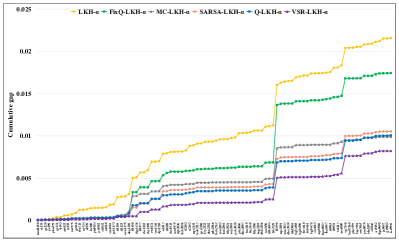
(a)

(b)

Figure 2: Comparison on the 94 small and hard TSP instances. Instances are sorted from left to right in ascending order of the number of the cities. (a) Results of algorithms with the $\alpha$-measure method. (b) Results of algorithms with the POPMUSIC method.

7.1.3 Ablation Study for VSR-LKH

In order to evaluate the effectiveness of the components in VSR-LKH, including the initial Q-value, the reinforcement learning method, and the variable reinforcement learning strategy, we compare VSR-LKH and LKH with their several variant algorithms. FixQ-LKH is a variant of LKH that replaces the initial candidate sets of LKH with the initial candidate sets generated according to the initial Q-value (see Section 5.3 for details). Q-LKH, SARSA-LKH, and MC-LKH are three variants of VSR-LKH that only use Q-learning, Sarsa, or Monte Carlo to update the Q-value, i.e., $M$ is fixed to be 1, 2, or 3 in Algorithm 2. We denote FixQ-LKH-$\alpha$ as the FixQ-LKH algorithm with the $\alpha$-measure method and Q-LKH-P as the Q-LKH algorithm with the POPMUSIC method, and so on.

We compare VSR-LKH, Q-LKH, SARSA-LKH, MC-LKH, FixQ-LKH, and LKH for solving the small and not easy instances, with a total of 94 instances. Figures 2a and 2b show the results of the algorithms with $\alpha$-measure and POPMUSIC, respectively. The results are expressed by the cumulative gap on the solution quality. We use the cumulants to express the results because it is more intuitive than comparing the results of each instance individually. Let $gap(j)=\frac{1}{10}\sum_{i=1}^{10}\frac{A_{i}-BKS_{j}}{BKS_{j}}$ be the average gap of calculating the $j$-th instance by an algorithm in 10 runs, where $A_{i}$ is the result of the $i$-th calculation and $BKS_{j}$ is the best-known solution of the $j$-th instance. The smaller the average gap, the closer the average solution is to the best-known solution. For an algorithm, $C_{gap}(j)=\sum_{i=1}^{j}gap(i)$ is the cumulative gap.

From the results in Figure 2, we can observe that:

(1) FixQ-LKH shows significantly better performance than LKH, indicating that the LKH algorithm with either the $\alpha$-measure or the POPMUSIC method can be improved significantly by simply replacing the $\alpha^{\pi}$-value or $\alpha$-value with our designed initial Q-value.

(2) Each of Q-LKH, SARSA-LKH, MC-LKH shows better performance than FixQ-LKH, indicating that the initial Q-value can be further improved by our reinforcement learning method with any of the three tested reinforcement learning algorithms. In other words, using an adaptive value trained by reinforcement learning to adjust the candidate sets is better than determining the candidate sets according to a fixed metric.

(3) Q-learning, Sarsa, and Monte Carlo show complementary performance in reinforcing LKH. When solving most of the 94 instances, Q-learning has the best performance in reinforcing LKH, followed by Sarsa and Monte Carlo. Thus we order Q-learning first and Monte Carlo last in VSR-LKH. Moreover, VSR-LKH outperforms Q-LKH, SARSA-LKH, and MC-LKH, indicating that our approach can combine the advantages of the three reinforcement learning methods and leverage their complementarity.

TABLE VI: Comparison of VSR-LKH-3, LKH-3, and GMA on Datasets I, II, and III. Best results appear in bold. The values in brackets beside some results are the average violation values of these solutions. A star in column Best indicates that a new best solution of the CTSP has been found.

Instances	$n$	$m$	BKS		GMA				LKH-3-$\alpha$				LKH-3-P				VSR-LKH-3-$\alpha$				VSR-LKH-3-P
					Best	Average	Time		Best	Average	Time		Best	Average	Time		Best	Average	Time		Best	Average	Time
Dataset I
eil21-2	21	2	144.92		144.92	144.92	0.05		144.92	144.92	0.00		144.92	144.92	0.00		144.92	144.92	0.00		144.92	144.92	0.00
eil21-3	21	3	157.48		157.48	157.48	0.06		157.48	157.48	0.00		157.48	157.48	0.00		157.48	157.48	0.00		157.48	157.48	0.00
eil31-2	31	2	259.36		259.36	259.36	0.08		259.36	259.36	0.02		259.36	259.36	0.02		259.36	259.36	0.01		259.36	259.36	0.01
eil31-3	31	3	295.31		295.31	295.31	0.10		295.31	295.31	0.01		295.31	295.31	0.01		295.31	295.31	0.01		295.31	295.31	0.00
eil31-4	31	4	315.97		315.97	315.97	0.09		315.97	315.97	0.04		315.97	315.97	0.14		315.97	315.97	0.02		315.97	315.97	0.02
eil41-2	41	2	346.24		346.24	346.24	0.10		346.24	346.24	0.01		346.24	346.24	0.01		346.24	346.24	0.02		346.24	346.24	0.01
eil41-3	41	3	367.84		367.84	367.84	0.11		367.84	367.84	0.05		367.84	367.84	0.02		367.84	367.84	0.01		367.84	367.84	0.03
eil41-4	41	4	392.14		392.14	392.14	0.09		392.14	392.14	0.03		392.14	392.14	0.05		392.14	392.14	0.01		392.14	392.14	0.01
eil51-2	51	2	478.08		478.08	478.08	0.11		478.08	478.08	0.25		478.08	478.08	0.19		478.08	478.08	0.06		478.08	478.08	0.14
eil51-3	51	3	469.50		469.50	469.50	0.12		469.50	469.50	0.44		469.50	469.50	0.17		469.50	469.50	0.28		469.50	469.50	0.27
eil51-4	51	4	489.99		489.99	489.99	0.14		489.99	489.99	0.06		489.99	489.99	0.05		489.99	489.99	0.01		489.99	489.99	0.01
eil51-5	51	5	525.98		525.98	525.98	0.10		525.98	525.98	0.15		525.98	525.98	0.09		525.98	525.98	0.02		525.98	525.98	0.06
eil76-3	76	3	593.28		593.28	593.28	0.10		593.28	593.28	0.04		593.28	593.28	0.11		593.28	593.28	0.05		593.28	593.28	0.05
eil76-4	76	4	603.79		603.79	603.79	0.16		603.79	603.79	0.02		603.79	603.79	0.03		603.79	603.79	0.02		603.79	603.79	0.02
eil76-5	76	5	651.99		651.99	651.99	0.11		651.99	651.99	3.49		651.99	651.99	1.46		651.99	651.99	0.82		651.99	651.99	0.47
eil76-6	76	6	672.73		672.73	672.73	0.11		672.73	672.73	0.15		672.73	672.73	0.19		672.73	672.73	0.11		672.73	672.73	0.06
eil101-4	101	4	726.82		726.82	726.82	0.09		726.82	726.82	0.08		726.82	726.82	0.07		726.82	726.82	0.03		726.82	726.82	0.04
eil101-5	101	5	779.15		779.15	779.15	0.08		779.15	779.36	14.12		779.15	779.22	9.32		779.15	779.15	3.56		779.15	779.15	3.99
eil101-6	101	6	759.55		759.55	759.55	0.17		759.55	759.55	0.14		759.55	759.55	0.07		759.55	759.55	0.02		759.55	759.55	0.11
eil101-7	101	7	798.85		798.85	798.85	0.18		798.85	798.85	0.10		798.85	798.85	0.17		798.85	798.85	0.04		798.85	798.85	0.03
Average	-	-	-		491.45	491.45	-		491.45	491.46	-		491.45	491.45	-		491.45	491.45	-		491.45	491.45	-
Dataset II
gr202-12	202	12	99871		99871	100124.35	308.96		99871	99871.00	7.45		99871	99871.00	7.53		99871	99871.00	4.54		99871	99871.00	3.67
gr202-25	202	25	173353		173358	173529.10	211.32		173353	173353.25	69.08		173353	173353.25	80.36		173353	173353.25	26.14		173353	173353.00	7.95
gr202-35	202	35	233749		233871	233987.05	99.48		233749	233749.00	37.15		233749	233749.00	11.14		233749	233749.00	4.78		233749	233749.00	3.77
gr229-10	229	10	222167		222167	222176.35	163.04		222167	222167.00	29.49		222167	222167.00	22.06		222167	222167.00	12.58		222167	222167.00	11.28
gr229-15	229	15	264146		264146	264149.90	85.40		264146	264146.00	73.70		264146	264153.40	111.12		264146	264146.00	21.99		264146	264146.00	34.51
gr229-20	229	20	319669		319669	319792.05	40.88		319669	319683.70	17.35		319669	319669.00	13.07		319669	319669.00	2.99		319669	319669.00	4.74
gr229-30	229	30	406664		406664	407410.15	37.88		406664	406664.00	24.32		406664	406664.00	91.88		406664	406664.00	15.83		406664	406664.00	20.95
gr431-12	431	12	248447		248447	248447.00	18.20		248447	248521.25	148.36		248447	248521.45	102.23		248447	248494.10	149.99		248447	248486.20	62.48
gr431-25	431	25	347335		347335	347457.00	284.44		347335	347923.35	220.90		347335	347729.55	157.18		347335	347414.20	144.73		347335	347481.80	186.57
gr431-40	431	40	415169		415311	415395.50	159.00		415169	415245.80	123.22		415169	415234.45	246.97		415169	415213.60	160.40		415169	415231.20	145.93
gr666-10	666	10	386157		386384	387662.35	513.88		386194	386897.25	214.97		386157	386782.90	242.02		386157	386521.60	316.64		386157	386787.85	238.09
gr666-15	666	15	445849		445869	446705.60	471.64		445849	445959.50	233.48		445849	446039.75	224.41		445849	445972.20	292.49		445849	445959.25	211.99
gr666-20	666	20	517842		518368	519211.75	537.00		517842	518275.90	304.88		517842	518233.80	359.33		517842	517897.20	268.48		517842	518082.40	317.52
gr666-30	666	30	649479		650306	650689.70	519.52		649479	649913.90	360.33		649613	649905.75	273.51		649479	649725.55	155.69		649479	649734.60	214.64
Average	-	-	-		337983.29	338338.42	-		337852.43	338026.49	-		337859.36	338005.31	-		337849.79	337918.41	-		337849.79	337955.88	-
Dataset III
pr1002-5	1002	5	313885		313867	313991.38	1745.48		*313848	314155.60	1407.23		313917	314405.90	1292.30		*313848	314079.35	709.25		*313848	314116.20	672.21
pr1002-10	1002	10	379846		379846	379974.21	827.44		*379627	379906.55	684.78		*379627	380029.80	839.67		*379627	379935.45	731.08		*379627	379959.05	566.98
pr1002-20	1002	20	514294		514887	515908.46	1003.20		*513415	513701.15	1113.93		*513415	514125.35	1381.40		*513415	513536.45	1179.89		*513415	513769.05	492.39
pr1002-30	1002	30	660999		661540	662432.28	1586.64		660999	661089.85	1133.29		660999	661002.30	1548.30		660999	661003.00	656.30		660999	661030.40	843.22
pr1002-40	1002	40	803398		803624	803626.41	776.76		*803365	803434.15	1675.16		*803365	803432.65	1292.27		*803365	803441.80	795.56		*803365	803377.45	814.01
fnl2461-3	2461	3	105505		105660	105750.91	1558.64		105295	105319.45	3085.18		105240	105295.60	2636.01		105215	105280.80	2934.89		*105211	105350.50	2797.08
fnl2461-6	2461	6	115271		116069	116187.21	2991.52		115340	115533.50	3042.90		115414	115592.85	3326.71		115397	115438.65	3189.77		115362	115428.50	3195.02
fnl2461-12	2461	12	142065		142836	143415.38	3461.32		142257	142401.10	3504.69		142472	142642.00	3443.95		142384	142750.10	3424.38		142211	142359.25	3415.15
fnl2461-24	2461	24	220379		220644	220987.34	3441.00		220801	220974.25	3350.23		220761	220979.95	3535.80		220633	221024.40	3448.49		220689	220783.80	3484.78
fnl2461-30	2461	30	266756		266916	267073.93	3470.36		266967	266983.70	3505.62		267027	267150.45	3486.34		266884	266994.00	3366.19		266848	267021.30	3382.15
fnl3461-3	3461	3	148917		148917	148967.06	1672.44		148677	148819.10	3220.53		148744	148881.50	3356.23		*148602	148727.45	3319.66		148861	149020.35	3230.14
fnl3461-6	3461	6	159934		159827	159973.41	2453.08		*159388	159476.40	3378.64		159407	159614.50	3386.49		159445	159601.40	3383.81		159471	159647.10	3338.94
fnl3461-12	3461	12	184681		185292	185442.08	3274.92		184963	184775.55	3428.76		185064	185188.05	3379.40		184796	184911.95	3220.92		184830	184912.25	3476.68
fnl3461-24	3461	24	262859		263452	263962.14	3485.12		263088	263235.50	3492.69		262962	263434.45	3520.24		263025	262899.05	3475.00		263073	263274.45	3361.28
fnl3461-30	3461	30	306584		307000	307164.67	3475.16		306780	306966.95	3512.19		306874	307041.05	3425.33		306639	306789.75	3401.25		306911	307029.35	3379.75
fnl3461-40	3461	40	384302		384542	384692.55	3500.72		384449	384467.35	3455.60		384344	384463.95	3479.15		384329	384453.95	3401.19		384386	384393.20	3373.22
pla5397-20	5397	20	38006100		*38005790	38017335.25	3052.76		38008251	(0.20) 38010979.00	3105.76		38012648	(0.30) 38024573.55	2820.13		38008497	38015636.25	2944.25		38037355	38063755.50	2695.47
pla5397-30	5397	30	51138000		*51132597	51137916.35	3260.36		51142260	(0.80) 51137200.80	3407.29		51147246	51157053.15	3389.76		51140446	(0.80) 51148566.60	3297.14		51154264	51168676.45	3438.23
pla5397-40	5397	40	64076083		64079810	64093104.85	3155.60		64115423	(0.10) 64205408.20	3502.70		64134218	(0.10) 64211186.40	3558.86		64112918	64203476.20	3514.61		64084778	64209839.25	3499.88
pla5397-50	5397	50	73993599		73993599	73993617.35	2370.56		73994497	74014644.50	2899.61		73993761	73999305.75	3031.65		73994274	73995734.95	1125.22		73993687	74015972.75	1617.12
pla5397-60	5397	60	85266200		85266247	85266635.70	3346.76		85327143	(0.50) 85385798.45	3455.18		85267770	(1.40) 85272672.90	3354.50		85266991	85355551.80	2372.33		85266829	85310489.75	2871.08
pla6397-20	6397	20	35807712		35913164	35962450.30	3151.76		36072330	(1.10) 36278639.45	3507.98		35997332	(2.45) 36142888.90	3507.43		35862883	35999858.55	3342.38		35894347	35972784.75	3454.74
pla6397-30	6397	30	47322010		47337789	47363407.50	3191.88		47409125	47529457.30	3518.43		47437109	47558752.85	3537.96		47351577	47418339.00	3497.80		47331593	47412878.80	3429.82
pla6397-40	6397	40	56638000		56630053	56642010.90	3250.40		56820404	(1.75) 56885941.25	3534.66		56751757	56801793.05	3521.46		56653970	56732131.15	3289.39		*56619860	56685429.80	3461.26
pla6397-50	6397	50	67161500		*67161326	67166462.35	3098.76		67269324	(0.80) 67396902.50	3554.62		67276880	67423848.70	3502.44		67221246	67294663.05	3418.47		67186365	67237839.15	3417.40
pla6397-60	6397	60	74791200		*74782803	74795802.45	3373.44		75241320	75677624.80	3100.88		74995813	(0.35) 75244288.65	3494.89		74838559	75065390.30	3326.20		74801384	(1.80) 74891708.50	3453.58
pla7397-20	7397	20	41066442		41233150	41361689.50	13295.32		41452981	(0.05) 41692029.00	14216.11		41255870	(1.40) 41341931.90	14243.41		*40936853	(1.80) 41095953.35	14140.48		41035540	(3.00) 41017604.30	14168.85
pla7397-30	7397	30	52636900		52559479	52683620.05	13750.32		52855404	(0.05) 52973298.15	14221.12		52877975	52908138.05	14246.43		*52502160	52617120.85	14151.87		52548091	52641236.45	14222.71
pla7397-40	7397	40	64937200		64892877	64957606.15	13599.92		65176228	(0.80) 65359193.95	14241.77		65154596	65343807.40	14276.59		64874922	(2.20) 64923282.15	14251.54		*64843070	64881685.20	14263.10
pla7397-50	7397	50	76311403		76244960	76345294.05	13796.32		76475226	(0.25) 76662535.55	14224.38		76522202	(2.80) 76771116.75	14325.48		76293837	76478400.10	14204.84		*76214793	76374032.05	14076.24
pla7397-60	7397	60	86153700		86099745	86145975.25	13799.24		86540779	86777244.80	13508.68		86377888	(0.70) 86473728.95	14305.98		86155989	86360702.70	14061.43		*86088267	(4.20) 85891430.10	14264.79
Average	-	-	-		29687364.74	29706854.11	-		29769998.52	(0.16) 61332459.85	-		29747506.35	(0.31) 61245005.80	-		29683345.97	(0.15) 29731473.37	-		29679655.81	(0.29) 29701510.81	-

7.2 Experimental Results for the TSPTW

This subsection first introduces the experimental setup, then presents the computational results of VSR-LKH-3 and the baseline algorithms for the TSPTW.

7.2.1 Experimental Setup

We compare VSR-LKH-3 with LKH-3 and other state-of-the-art heuristics for the TSPTW, including the GVNS algorithm [1] and the VIG_VNS algorithm [2]. The results of GVNS and VIG_VNS are from the literature. The GVNS was run on a Pentium 4 2.40 GHz processor. The VIG_VNS was run on an Intel Core i5 2.53 GHz processor.

We compare the algorithms in solving the TSPTW on the benchmark instances proposed by [27, 1, 42, 43], with a total of 425 instances. Each instance is solved 10 times by each algorithm. We divide these instances into three sets:

• Dataset A: This dataset [42] contains 135 instances with 20 to 200 cities grouped in 27 test cases. Each group has five Euclidean instances, coordinates between 0 and 50, with the same number of cities and the same maximum range of time windows.

• Dataset B: This dataset [27, 43] contains 165 instances with 20 to 200 cities grouped in 33 test cases. This set of instances, in the majority, are the instances proposed by Dumas et al. [42] with wider time windows, systematically extended by 100.

• Dataset C: This dataset [1] contains 125 instances with 200 to 400 cities grouped in 25 test cases. It contains relatively large-scale instances that can distinguish the performance of different heuristics.

The cut-off time $T_{max}$ and the maximum number of iterations $I_{max}$ are set to $n/10$ seconds and $+\infty$, respectively, in VSR-LKH-3 and LKH-3 for the TSPTW. The parameters related to reinforcement learning in VSR-LKH-3 include the learning rate $\lambda_{2}$, the reward discount factor $\gamma_{2}$, and the variable strategy parameter $N_{max}$. We set $\lambda_{2}=0.1$ and $\gamma_{2}=0.9$ as VSR-LKH does. For the variable strategy parameter, since VSR-LKH-3 does not restrict the maximum number of iterations, we use the running time to control the switching of the reinforcement learning algorithm in VSR-LKH-3. That is, changing the reinforcement learning algorithm when the best solution has not been improved for $T_{max}/20$ seconds.

7.2.2 Comparison on VSR-LKH-3 with TSPTW Baselines

The comparison results on VSR-LKH-3 with LKH-3, GVNS, and VIG_VNS are shown in Table IV. Since the instances in Datasets A and B are too simple to distinguish the performance of the algorithms, we only present the average values of the best and average solutions of the algorithms on these two benchmarks in Table IV. For the instances in Datasets C, we present the average values of the best and average solutions of the five instances in each group of instances. The values in brackets beside some results are the average violation values of these solutions. Column $w$ is the width of the time windows. Column BKS is the best-known solution reported by [1, 2, 15].

In order to show the advantage of VSR-LKH-3 over the baselines in solving the TSPTW more clearly, we summarize the comparative results between VSR-LKH-3 and each baseline algorithm in Table V. The comparative results are based on all the 85 compared groups of instances.

From the results in Tables IV and V, we can observe that:

(1) The algorithms with the POPMUSIC method show significantly lower performance than the algorithms with the $\alpha$-measure. This might be because the POPMUSIC is not good at solving the problems with time window constraints. Moreover, the results of VSR-LKH-3-P are significantly better than those of LKH-3-P, indicating that our proposed reinforcement learning method and the reward function that considers the penalty function are effective.

(2) When solving the TSPTW, VSR-LKH-3 also significantly outperforms LKH-3 with either the $\alpha$-measure or the POPMUSIC method. Moreover, the best (average) solutions of VSR-LKH-3-$\alpha$ are better than those of GVNS in 16 (36) instances, and worse than those of GVNS in one instance (6 instances). The best (average) solutions of VSR-LKH-3-$\alpha$ are better than those of VIG_VNS in 6 (25) instances, and worse than those of VIG_VNS in 0 (8) instances, indicating a significant improvement.

7.3 Experimental Results for the CTSP

This subsection first introduces the experimental setup, and then presents the computation results of VSR-LKH-3 and the baseline algorithms for the CTSP.

TABLE VII: Summarized comparisons for the CTSP.

Algorithm pair	Indicator	#Wins	#Ties	#Losses
VSR-LKH-3-$\alpha$ vs. GMA	Best	27	27	11
	Average	29	20	16
VSR-LKH-3-P vs. GMA	Best	30	27	8
	Average	28	20	17
VSR-LKH-3-$\alpha$ vs. LKH-3-$\alpha$	Best	23	38	4
	Average	29	25	11
VSR-LKH-3-P vs. LKH-3-P	Best	21	37	7
	Average	31	24	10

7.3.1 Experimental Setup

There are several effective heuristic algorithms for the CTSP proposed recently [31, 29, 4]. Among these algorithms, the GMA algorithm [4] based on the famous EAX crossover method [26] significantly outperforms the other heuristics. Therefore, we choose LKH-3 and GMA as the baseline algorithms for the CTSP. The results of GMA are obtained by running its source code on our machine.

We tested the algorithms for the CTSP on the benchmark instances introduced by [3, 29, 44, 45] and used by [31, 4], with a total of 65 instances. Each instance is solved 20 times by each algorithm as in [4]. Also, we divide these instances into three sets as in [4]:

• Dataset I: This dataset [3] contains 20 small instances with 21 to 101 cities, generated from six graphs by varying the number of routes and exclusive cities in each instance. The number of salesmen is between 2 and 7.

• Dataset II: This dataset contains 14 medium instances with 202 to 666 cities, generated from four graphs. The number of salesmen is between 10 and 40. The 6 instances related to the two graphs with 202 and 431 cities were from [44], while the remaining instances were presented in [29].

• Dataset III: This dataset contains 31 large instances with 1,002 to 7,397 cities, generated from six graphs. The number of salesmen is between 3 and 60. The 5 instances related to the first graph were presented in [44], and the remaining instances in [45].

We set the cut-off time $T_{max}$ for each instance of VSR-LKH-3 and LKH-3 for the CTSP the same as He et al. [31] does. That is, $T_{max}$ is set to 1, 10, and 60 minutes for Dataset I, II, and III, respectively, except $T_{max}=240$ minutes for large instances with more than 7,000 cities. The parameters related to reinforcement learning in VSR-LKH-3 for the CTSP are set to the same as those in VSR-LKH-3 for the TSPTW (see Section 7.2.1 for details).

7.3.2 Comparison on VSR-LKH-3 with CTSP Baselines

The comparison results on VSR-LKH-3 with LKH-3 and GMA are shown in Table VI. We compare the best and average solutions in 10 runs obtained by these algorithms. Column $m$ is the number of the salesmen. Column BKS is the best-known solution reported by [4, 15]. The values in brackets beside some results are the average violation values of these solutions. A star in column Best indicates that a new best solution of the CTSP has been found. We also summarize the comparative results between VSR-LKH-3 and each baseline algorithm for the CTSP in Table VII. The comparative results are based on all the 65 compared instances.

From the results in Tables VI and VII, we observe that:

(1) The best (average) solutions of VSR-LKH-3-$\alpha$ are better than those of LKH-3-$\alpha$ in 23 (29) instances, and worse than those of LKH-3-$\alpha$ in 4 (11) instances. The best (average) solutions of VSR-LKH-3-P are better than those of LKH-3-P in 21 (31) instances, and worse than those of LKH-3-P in 7 (10) instances. The results demonstrate that when solving the CTSP, VSR-LKH-3 also significantly outperforms LKH-3 with either the $\alpha$-measure or the POPMUSIC method.

(2) Both VSR-LKH-3-$\alpha$ and VSR-LKH-3-P significantly outperforms the advanced GMA heuristic algorithm for the CTSP. In particular, the performance of either LKH-3-$\alpha$ or LKH-3-P is weaker than GMA. Our proposed reinforcement learning method can help LKH-3 outperform GMA, indicating the excellent performance of our proposed method.

(3) VSR-LKH-3 provides 12 new best solutions for the 65 tested CTSP instances. In particular, VSR-LKH-3 provides the new best solutions for all the 5 large instances with more than 7,000 cities, indicating that our proposed algorithm is efficient and effective for large CTSP instances.

TABLE VIII: Comparison of VSR-LKH-3 and VSR-LKH-3-NoV.

Algorithm\Benchmark	Dataset C			Dataset III
	Best	Average		Best	Average
VSR-LKH-3-NoV-$\alpha$	(0.08) 12135.36	(3.32) 12136.43		29705510.29	(0.24) 29802623.93
VSR-LKH-3-$\alpha$	12135.4	(0.40) 12136.65		29683345.97	(0.15) 29731473.37
VSR-LKH-3-NoV-P	12138.4	(163277.04) 89453.64		29685164.71	(0.61) 29711676.82
VSR-LKH-3-P	12137.5	(77353.64) 46503.25		29679655.81	(0.29) 29701510.81

7.4 Ablation Study for VSR-LKH-3

In order to demonstrate that our designed reward function in VSR-LKH-3 is effective and reasonable, we compare VSR-LKH-3 with its variant VSR-LKH-3-NoV for solving the TSPTW and CTSP. VSR-LKH-3-NoV is a variant of VSR-LKH-3 with the reward function in VSR-LKH (Eq. 3), i.e., without considering the violation function.

We compare VSR-LKH-3 with VSR-LKH-3-NoV in solving the TSPTW instances of Dataset C and the CTSP instances of Dataset III. The results are shown in Table VIII. Due to the limited space, we provide the average values of the best and average solutions of the algorithms. From the results we can see that with either the $\alpha$-measure or the POPMUSIC method, VSR-LKH-3 significantly outperforms VSR-LKH-3-NoV. The average violation values of the solutions obtained by VSR-LKH-3 are smaller than VSR-LKH-3-NoV, indicating that the designed reward function can help the algorithm find feasible solutions more easily, so as to find better solutions.

8 Conclusion

We combine reinforcement learning with the powerful heuristic local search methods, LKH and LKH-3, for solving the TSP and its variant problems. We first propose a variable strategy reinforced algorithm called VSR-LKH for the TSP, and then propose another algorithm called VSR-LKH-3 that combines the variable strategy reinforcement learning method with LKH-3 for the TSP variants. These approaches use a Q-value as the metric for selecting and sorting the candidate cities, and allow the program to learn to select appropriate edges to be added from the candidate sets through reinforcement learning.

The variable strategy reinforced methods in VSR-LKH and VSR-LKH-3 combine the advantages of three reinforcement learning algorithms, Q-learning, Sarsa, and Monte Carlo, so as to further improve the flexibility and robustness of the proposed algorithms. VSR-LKH-3 further benefits from the new reward function based on the violation function for evaluating the infeasibility of the solutions, which enables the algorithm to find high-quality and feasible solutions more efficiently. Extensive experiments on public benchmarks show that with either the $\alpha$-measure or the POPMUSIC method for determining the candidate sets, VSR-LKH (VSR-LKH-3) significantly outperforms the LKH (LKH-3) algorithm for solving the TSPs. Moreover, our proposed reinforcement learning method can help LKH-3 outperform the state-of-the-art CTSP heuristic, creating 12 new records among the 65 public CTSP instances.

VSR-LKH and VSR-LKH-3 essentially reinforce the $k$-opt process of LKH and LKH-3. Hence, other algorithms based on $k$-opt could also be strengthened by our methods. Furthermore, our work demonstrates the feasibility and effectiveness of incorporating reinforcement learning with heuristic algorithms in solving various combinatorial optimization problems.

References

- [1] R. F. da Silva and S. Urrutia, “A general VNS heuristic for the traveling salesman problem with time windows,” Discrete Optimization, vol. 7, no. 4, pp. 203–211, 2010.
- [2] K. Karabulut and M. F. Tasgetiren, “A variable iterated greedy algorithm for the traveling salesman problem with time windows,” Information Sciences, vol. 279, pp. 383–395, 2014.
- [3] J. Li, M. Zhou, Q. Sun, X. Dai, and X. Yu, “Colored traveling salesman problem,” IEEE Transactions on Cybernetics, vol. 45, no. 11, pp. 2390–2401, 2015.
- [4] P. He, J. Hao, and Q. Wu, “Grouping memetic search for the colored traveling salesmen problem,” Information Sciences, vol. 570, pp. 689–707, 2021.
- [5] M. Nazari, A. Oroojlooy, L. V. Snyder, and M. Takác, “Reinforcement learning for solving the vehicle routing problem,” in The 31st Annual Conference on Neural Information Processing Systems, NeurIPS, 2018, pp. 9861–9871.
- [6] J. Li, X. Meng, and X. Dai, “Collision-free scheduling of multi-bridge machining systems: a colored traveling salesman problem-based approach,” IEEE/CAA Journal of Automatica Sinica, vol. 5, no. 1, pp. 139–147, 2018.
- [7] P. He, J. Li, D. Zhang, and S. Wan, “Optimisation of the harvesting time of rice in moist and non-moist dispersed fields,” Biosystems Engineering, vol. 170, pp. 12–23, 2018.
- [8] E. B. Khalil, H. Dai, Y. Zhang, B. Dilkina, and L. Song, “Learning combinatorial optimization algorithms over graphs,” in The 30th Annual Conference on Neural Information Processing Systems, NIPS, 2017, pp. 6348–6358.
- [9] S. Lin and B. W. Kernighan, “An effective heuristic algorithm for the traveling-salesman problem,” Operations Research, vol. 21, no. 2, pp. 498–516, 1973.
- [10] O. C. Martin, S. W. Otto, and E. W. Felten, “Large-step markov chains for the traveling salesman problem,” Complex Systems, vol. 5, no. 3, 1991.
- [11] K. Helsgaun, “An effective implementation of the lin-kernighan traveling salesman heuristic,” European Journal of Operational Research, vol. 126, no. 1, pp. 106–130, 2000.
- [12] É. D. Taillard and K. Helsgaun, “POPMUSIC for the travelling salesman problem,” European Journal of Operational Research, vol. 272, no. 2, pp. 420–429, 2019.
- [13] S. Lin, “Computer solutions of the traveling salesman problem,” Bell System Technical Journal, vol. 44, no. 10, pp. 2245–2269, 1965.
- [14] M. Held and R. M. Karp, “The traveling-salesman problem and minimum spanning trees,” Operations Research, vol. 18, no. 6, pp. 1138–1162, 1970.
- [15] K. Helsgaun, “An extension of the lin-kernighan-helsgaun tsp solver for constrained traveling salesman and vehicle routing problems,” Roskilde University, Tech. Rep., 2017.
- [16] R. Jonker and T. Volgenant, “Transforming asymmetric into symmetric traveling salesman problems: erratum,” Operations Research Letters, vol. 5, no. 4, pp. 215–216, 1986.
- [17] M. R. Rao, “Technical note—a note on the multiple traveling salesmen problem,” Operations Research, vol. 28, no. 3-part-i, pp. 628–632, 1980.
- [18] R. Jonker and T. Volgenant, “Technical note - an improved transformation of the symmetric multiple traveling salesman problem,” Operations Research, vol. 36, no. 1, pp. 163–167, 1988.
- [19] R. S. Sutton and A. G. Barto, Reinforcement learning - an introduction, ser. Adaptive computation and machine learning. MIT Press, 1998.
- [20] J. Zou, T. Hao, C. Yu, and H. Jin, “A3C-DO: A regional resource scheduling framework based on deep reinforcement learning in edge scenario,” IEEE Transactions on Computers, vol. 70, no. 2, pp. 228–239, 2021.
- [21] Y. Li, X. Wang, H. Liu, L. Pu, S. Tang, G. Wang, and X. Liu, “Reinforcement learning-based resource partitioning for improving responsiveness in cloud gaming,” IEEE Transactions on Computers, vol. 71, no. 5, pp. 1049–1062, 2022.
- [22] N. Mladenovic and P. Hansen, “Variable neighborhood search,” Computers & Operations Research, vol. 24, no. 11, pp. 1097–1100, 1997.
- [23] J. Zheng, K. He, J. Zhou, Y. Jin, and C. Li, “Combining reinforcement learning with lin-kernighan-helsgaun algorithm for the traveling salesman problem,” in The 35th AAAI Conference on Artificial Intelligence, AAAI, 2021, pp. 12 445–12 452.
- [24] L. Xin, W. Song, Z. Cao, and J. Zhang, “Neurolkh: Combining deep learning model with lin-kernighan-helsgaun heuristic for solving the traveling salesman problem,” in The 34th Annual Conference on Neural Information Processing Systems, NeurIPS, 2021, pp. 7472–7483.
- [25] Y. Nagata, “New EAX crossover for large TSP instances,” in Parallel Problem Solving from Nature - PPSN IX, vol. 4193, 2006, pp. 372–381.
- [26] Y. Nagata and S. Kobayashi, “A powerful genetic algorithm using edge assembly crossover for the traveling salesman problem,” INFORMS Journal on Computing, vol. 25, no. 2, pp. 346–363, 2013.
- [27] J. W. Ohlmann and B. W. Thomas, “A compressed-annealing heuristic for the traveling salesman problem with time windows,” INFORMS Journal on Computing, vol. 19, no. 1, pp. 80–90, 2007.
- [28] X. Meng, J. Li, M. Zhou, X. Dai, and J. Dou, “Population-based incremental learning algorithm for a serial colored traveling salesman problem,” IEEE Transactions on Systems, Man, and Cybernetics: Systems, vol. 48, no. 2, pp. 277–288, 2018.
- [29] V. Pandiri and A. Singh, “A swarm intelligence approach for the colored traveling salesman problem,” Applied Intelligence, vol. 48, no. 11, pp. 4412–4428, 2018.
- [30] X. Meng, J. Li, X. Dai, and J. Dou, “Variable neighborhood search for a colored traveling salesman problem,” IEEE Transactions on Intelligent Transportation Systems, vol. 19, no. 4, pp. 1018–1026, 2018.
- [31] P. He and J. Hao, “Iterated two-phase local search for the colored traveling salesmen problem,” Engineering Applications of Artificial Intelligence, vol. 97, p. 104018, 2021.
- [32] I. Bello, H. Pham, Q. V. Le, M. Norouzi, and S. Bengio, “Neural combinatorial optimization with reinforcement learning,” in The 5th International Conference on Learning Representations, ICLR, 2017.
- [33] Y. L. Goh, W. S. Lee, X. Bresson, T. Laurent, and N. Lim, “Combining reinforcement learning and optimal transport for the traveling salesman problem,” CoRR, vol. abs/2203.00903, 2022.
- [34] M. Cuturi, “Sinkhorn distances: Lightspeed computation of optimal transport,” in The 27th Annual Conference on Neural Information Processing Systems, NIPS, 2013, pp. 2292–2300.
- [35] R. Zhang, A. Prokhorchuk, and J. Dauwels, “Deep reinforcement learning for traveling salesman problem with time windows and rejections,” in 2020 International Joint Conference on Neural Networks, IJCNN, 2020, pp. 1–8.
- [36] G. Wu, Z. Zhang, H. Liu, and J. Wang, “Solving time-dependent traveling salesman problem with time windows with deep reinforcement learning,” in 2021 IEEE International Conference on Systems, Man, and Cybernetics, SMC, 2021, pp. 558–563.
- [37] F. Liu and G. Zeng, “Study of genetic algorithm with reinforcement learning to solve the TSP,” Expert Systems with Applications, vol. 36, no. 3, pp. 6995–7001, 2009.
- [38] P. R. de O. da Costa, J. Rhuggenaath, Y. Zhang, and A. Akcay, “Learning 2-opt heuristics for the traveling salesman problem via deep reinforcement learning,” in The 12th Asian Conference on Machine Learning, ACML, vol. 129, 2020, pp. 465–480.
- [39] J. Sui, S. Ding, R. Liu, L. Xu, and D. Bu, “Learning 3-opt heuristics for traveling salesman problem via deep reinforcement learning,” in The 13th Asian Conference on Machine Learning, ACML, vol. 157, 2021, pp. 1301–1316.
- [40] J. Zhao, M. Mao, X. Zhao, and J. Zou, “A hybrid of deep reinforcement learning and local search for the vehicle routing problems,” IEEE Transactions on Intelligent Transportation Systems, vol. 22, no. 11, pp. 7208–7218, 2021.
- [41] M. Held and R. M. Karp, “The traveling-salesman problem and minimum spanning trees: Part II,” Mathematical Programming, vol. 1, no. 1, pp. 6–25, 1971.
- [42] Y. Dumas, J. Desrosiers, É. Gélinas, and M. M. Solomon, “An optimal algorithm for the traveling salesman problem with time windows,” Operations Research, vol. 43, no. 2, pp. 367–371, 1995.
- [43] M. Gendreau, A. Hertz, G. Laporte, and M. Stan, “A generalized insertion heuristic for the traveling salesman problem with time windows,” Operations Research, vol. 46, no. 3, pp. 330–335, 1998.
- [44] X. Dong, W. Dong, and Y. Cai, “Ant colony optimization for coloured travelling salesman problem by multi-task learning,” IET Intelligent Transport Systems, vol. 12, no. 8, pp. 774––782, 2018.
- [45] X. Dong, Q. Lin, M. Xu, and Y. Cai, “Artificial bee colony algorithm with generating neighbourhood solution for large scale coloured traveling salesman problem,” IET Intelligent Transport Systems, vol. 13, no. 10, pp. 1483––1491, 2019.