UDRN: Unified Dimensional Reduction Neural Network for Feature Selection and Feature Projection

Abstract

Dimensional reduction (DR) maps high-dimensional data into a lower dimensions latent space with minimized defined optimization objectives. The two independent branches of DR are feature selection (FS) and feature projection (FP). FS focuses on selecting a critical subset of dimensions but risks destroying the data distribution (structure). On the other hand, FP combines all the input features into lower dimensions space, aiming to maintain the data structure; but lacks interpretability and sparsity. Moreover, FS and FP are traditionally incompatible categories and have not been unified into an amicable framework. Therefore, we consider that the ideal DR approach combines both FS and FP into a unified end-to-end manifold learning framework, simultaneously performing fundamental feature discovery while maintaining the intrinsic relationships between data samples in the latent space. This paper proposes a unified framework named Unified Dimensional Reduction Network (UDRN) to integrate FS and FP in an end-to-end way. Furthermore, a novel network framework is designed to implement FS and FP tasks separately using a stacked feature selection network and feature projection network. In addition, a stronger manifold assumption and a novel loss function are proposed. Furthermore, the loss function can leverage the priors of data augmentation to enhance the generalization ability of the proposed UDRN. Finally, comprehensive experimental results on four image and four biological datasets, including very high-dimensional data, demonstrate the advantages of DRN over existing methods (FS, FP, and FS&FP pipeline), especially in downstream tasks such as classification and visualization.

1 Introduction

Dimensional reduction (DR) [1, 2, 3] transforms a high-dimensional (h-dim) data into an intrinsic low-dimensional (l-dim) embedding. The performance of typical classification or visualization methods degrades when data has too many features. Therefore, DR is introduced to overcome this issue. DR have a broad range of applications in signal processing [4], speech recognition [5], neuroinformatics [6], and bioinformatics [7].

The ideal DR method is expected to have two characteristics [8]. (1) Structural maintainability. The local structures of the data need to be preserved from being broken while reducing the data dimensionally. Under the manifold assumption, ensuring the local connectivity of the data is the golden rule for structure preservation. (2) Sparse interpretability. Redundant features and noisy features need to be identified while reducing the data dimensionally. It is because these useless features can affect the accuracy of downstream tasks.

In many biology exploration fields, such as single-cell analysis [9, 10, 11] genomics [12] and proteomics [13], DR is required to have both characteristics. However, the current DR methods cannot achieve the above characteristics with a unified framework. The current DR methods often contain two incompatible branches, feature projection (FP) [14] and feature selection (FS) [15]. FP methods concentrate on structural maintainability. They produce new variables obtained from the original features via an arbitrarily complex mapping, thus having better distinguish and structure-preserving performance. In contrast, FS methods concentrate on sparse interpretability. They allow the user to find an essential feature subset during the generalization phase of the model but often break the structure of the data by losing features [16, 17, 18].

Due to the needs of practical fields such as biology exploration, some researchers build pipeline methods by splicing the FS and FP methods together to solve the above issues [19, 11, 13]. However, these pipeline methods are not satisfying due to the following reasons. (1) Inconsistent optimization objective. The stacked approach of FS and FP may introduce conflicting objectives, e.g., FS focuses on reconstruction error while FP focuses on distance/similarity preserving. The DR method that can combine both FS and FP has not been found yet. (2) Weak generalizability. FS and FP are mainly applied in scenarios with a huge number of features, where it is easy to fall into overfitting due to the relatively small number of samples.

In this paper, an end-to-end Unified Dimensional Reduction Network, named UDRN, is designed to perform feature selection and projection (FS&FP) in a unified framework. To design consistent optimization objective, a novel neural network framework is designed. The framework includes a feature selection network (FS network) and feature projection network (FP network) for both FS and FP tasks. The gate layer of the FS network mask off unimportant features and generate feature subset during the forward propagation process, thus implementing online feature selection and enabling the following FP with selected features. The FP network then maps the feature subset to l-dim space for downstream tasks such as classification and visualization. To improve the generalizability of UDRN, a manifold connectivity [20, 21] based manifold assumption using priors of data augmentation is proposed. Furthermore, based on the above assumption, a novel loss function is designed to train the FS&FP neural network with online generated augmented data. The proposed unsupervised loss function is compatible with the new data generated by data augmentation, thus allowing a finer depiction of the data manifold and ultimately leading to improved performance.

To the best of our knowledge, UDRN is the first attempt to apply data augmentation-compatible structure-preserving loss functions on the neural network for the FS&FP task. Our contributions are summarized as follows.

• A unified FS&FP task and a novel neural network framework. We explicitly define the FS&FP task and design a neural network framework with a unified objective to solve this task. The proposed task is extensively employed in biology, genomics, and proteomics.

• A manifold connectivity assumption under augmented data and corresponding novel loss function. We propose a novel structure-preserving loss function and online data augmentation to provide a consistent and generalizable objective function.

• Extensive experiments and promising results. We compare UDRN with state-of-the-art FS, FP, and FS&FP pipeline methods on ten datasets and a case study of the supervised scenarios.

2 Related Work

2.1 Feature Selection (FS)

The FS methods include four categories [22], (a) filter methods, which are independent of learning models; (b) wrapper methods, which rely on learning models for selection criteria; (c) embedder methods, which embed the FS into learning models to also achieve model fitting simultaneously; (d) hybrid approaches, which are a combination of more than one of the above three. Unsupervised FS is more widely used because it does not require information about the label. At the same time, unsupervised FS is more challenging due to the same reasons [23, 24].

From another perspective, FS methods can be divided into non-parametric and parametric methods. Non-parametric models select the appropriate features based on statistics. For example, Laplacian score (LS) [25] uses the nearest neighbor graph to model the local geometric structures of the data. Principal feature analysis (PFA) [26] utilizes the structure of the main components of a set of features to select the subset of relevant features. Multi-cluster feature selection (MCFS) [27] selects a subset of features to cover the multi-cluster structure of the data, where spectral analysis is used to find the inter-relationship between different components. In Unsupervised discriminative feature selection (UDFS) [28], the discriminatory analysis method and $\ell_{2,1}$ regularization are used to identify the valuable features. Nonnegative discriminative feature selection (NDFS) [29] select discriminative features by learning the cluster labels and FS matrix. The NDFS uses a nonnegative constraint on the class indicator to understand cluster labels and adopts an $\ell_{2,1}$ limitation on the redundant features. IVFS [16] select useful features by preserving the pairwise distances, as well as topological patterns, of the complete data.

Parametric models select the appropriate features based on neural networks. For example, Autoencoder Feature Selector (AEFS) [30] combines reconstruction loss and $\ell_{2,1}$ regularization loss to obtain a subset of useful features on the weights of the encoder. The agnostic feature selection (AgnoS) [31] combines AE with different auxiliary tasks to design a range of FS methods. Such as AgnoS-W: the $\ell_{2,1}$ norm on the weights of the first layer of AE, AgnoS-G: $\ell_{2,1}$ norm on the gradient of the encoder, and AgnoS-S: $\ell_{1}$ norm on the slack variables that constitute the first layer of AE. Concrete Autoencoders (CAE) [17] replaces the first hidden layer of AE with a concrete selector layer, which is the relaxation of a discrete distribution called concrete distribution [32]. Fractal Autoencoders (FAE) [18] extends autoencoders by adding a one-to-one scoring layer. FAE uses a small sub-neural network for FS in an unsupervised fashion. Atashgahi et.al [33] introduce the strength of the neuron in sparse neural networks as a criterion to measure the feature importance and designs QuickSelection (QS).

We consider that it is a meaningful research direction for designing FS methods based on neural networks. Training FS models based on reconstruction loss cannot take into account structure preservation & feature projection; thus, it is meaningful to design novel structure-preserving loss functions for both FS and FP tasks.

2.2 Feature Projection (FP)

In recent years, Numerous manifold-learning-based FP methods have been proposed. Some of the FP methods are based on the manifold assumption [34, 35], which states that a pattern of interest in data is a lower-dimensional manifold (or hyper-surface) residing in the high dimensional data space. When the data contains multiple manifolds, the geometric structure usually includes the local system of neighboring points on each manifold and global relationships among different manifolds.

FP methods can be divided into non-parametric and parametric methods. In terms of non-parametric methods, Isometric Mapping (ISOMAP) [36] and Locally Linear Embedding (LLE) [37] are classic ones, among others. Later developments include Hessian LLE (HLLE) [38], Modified LLE (MLLE) [39]. The t-Distributed Stochastic Neighbor Embedding (t-SNE) [40] and Uniform Manifold Approximation and Projection (UMAP) [41] are two popular methods for manifold learning-based Nonlinear dimensionality reduction (NLDR), widely used for NLDR and visualization. The t-SNE improves the previous work of SNE [42] by using a long-tailed $t$-distribution for the embedding layer [40]. The UMAP further introduces a global term added to the local neighborhood-based t-SNE to preserve the global structure.

In terms of parametric methods, the Deep Isometric Manifold Learning (DIMAL) [43] combines a deep learning framework with a multi-dimensional scaling (MDS) objective, which can be seen as a neural network version of MDS. DIMAL learns distance-preserving mapping to generate low-dimensional embeddings for a particular class of manifolds with sparse geodesic sampling. Topological Autoencoder (TAE) [44] imposes topological constraints [45] on top of the autoencoder architecture to preserve the topological structure of data. Sainburg et.al [46] extend the embedding step of UMAP [41] to a parametric optimization over neural network weights, learning a parametric relationship between data and embedding. DLME [47] is a generalizable neural network with manifold flatness assumption which can handle biological and image data well.

2.3 FS and FP (FS&FP) Piplines

Some pipeline methods are designed to combine feature selection and feature projection in fields such as bioinformatics (in single-cell analysis [48, 9, 10, 11], genomics [49, 12], and proteomics [50, 13]). The pipeline method includes an FS method, which discovers the significant features, and an FP method, which analyzes the effects of these features on phenotype. Since no corresponding end-to-end FS and FP analysis methods can be found, such tasks are often performed using a pipeline approach. For example, different FS and FP methods are used in series to complete the analysis task [51, 52, 53].

As demonstrated above, the pipeline approach may cause corruption of helpful information due to the non-uniform loss functions and interrupted information flow of FS and FP. Therefore, we innovatively propose UDRN based on a neural network, which accomplishes feature selection and projection through an end-to-end network framework.

3 Problem Defenition and Preliminaries

3.1 Problem Definition

We use bold uppercase characters for matrices (e.g., $\bm{A}$), bold lowercase characters for vectors (e.g., $\bm{a}$), and regular lowercase characters for scalars (e.g., $a$). Also, we represent the $i$-th element of vector $\bm{a}$ as $a_{i}$, the $i$-th row of matrix $\bm{A}$ as $A_{i*}$, the $j$-th column of matrix $\bm{A}$ as $A_{*j}$, the $(i,j)$-th entry of matrix $\bm{A}$ as $A_{ij}$, the transpose of $\bm{A}$ as $\bm{A}^{T}$. We introduce our proposed concept on the attributed graph [54] to precisely describe our data augmentation and loss function and adapt it to a broader range of situations.

Definition 3.1 (Attributed Graph). Let graph $\bm{\mathcal{G}}(\bm{\mathcal{V}},\bm{\mathcal{E}},\bm{\mathcal{X}})$ be an attributed graph (network). It consists of - (1) $\bm{\mathcal{V}}$, the set of nodes, $n=|\bm{\mathcal{V}}|$, where $n$ is the number of the nodes. (2) $\bm{\mathcal{E}}$, the set of edges, $e=|\bm{\mathcal{E}}|$, where $e$ is the number of the edges. and (3) $\bm{\mathcal{X}}=[\bm{x}_{1},\bm{x}_{2},\ldots,\bm{x}_{n}]$, the set of node attributes (features), where $\bm{x}_{i}\in\mathcal{R}^{\mathcal{D}}$, $\mathcal{D}$ is the dimensional number of attribute.

With the definition of the attributed graph, we now define the FS&FP problem as follows.

Definition 3.2 (FS&FP Task on Attributed Graph). Given an attributed network $\bm{\mathcal{G}}(\bm{\mathcal{V}},\bm{\mathcal{E}},\bm{\mathcal{X}})$, the FS&FP task on attributed graph aims to (a) select a subset of $d$ features from the original $\mathcal{D}$-dimensional feature space, and $d\ll\mathcal{D}$ and then (b) map the data with selected features $\bm{\mathcal{X}}^{s}$ to a latent space $\bm{\mathcal{Z}}$. We expect that the selected feature subsets and the generated embedding representations imply as much information as possible as the original data. It may manifest itself in as high an accuracy as possible in downstream tasks, neighborhood structure maintenance, and consistent visualization output.

The adjacency of nodes is described by the edges of the attribute graph, which contains critical a priori knowledge. In the unsupervised context, $k$-NN is used to build the edge structure.

$$\bm{\mathcal{E}}=\{(\bm{v}_{i},\bm{v}_{j})|\bm{v}_{j}\in\mathcal{N}^{k}(\bm{v}_{i}),\bm{v}_{i}\in\bm{\mathcal{V}}\}$$ (1)

where $\mathcal{N}^{k}(\bm{v}_{i})$ is set of $k$-NN neighborhood of node $\bm{v}_{i}$, $k$ is the hyperparameter of $k$-NN. UDRN can be easily compatible with the supervised situation because the methods and problems are based on attribute graphs. When additional supervised information or structural information is accessible, we only need to redefine the edges.

$$\bm{\mathcal{E}}=\{(\bm{v}_{i},\bm{v}_{j})|\bm{v}_{j}\in\mathcal{N}^{k}(\bm{v}_{i})\cap Y(\bm{v}_{i}),\bm{v}_{i}\in\bm{\mathcal{V}}\}$$ (2)

where $Y(\bm{v}_{i})$ is the set of nodes with the same label as $\bm{v}_{i}$.

3.2 AE-based Feature Selection

AE-based FS methods add a superficial one-to-one layer between the input and hidden layers, which can weigh the importance of each feature [30, 17, 18]. The parameters of the one-to-one layer are trained by $L_{1}$ regularization loss and reconstruction loss, thus these methods highlight the features which friendly to reconstruction. The loss function of AE-based FS is,

$$L_{\text{fp}}=\min_{\bm{\mathcal{W}},f,g}\left\|{\bm{x}}-g\left(f\left(\bm{x}\bm{\mathcal{W}}\right)\right)\right\|_{\mathrm{F}}^{2}+\lambda_{1}{L}_{1}(\bm{w})$$ (3)

where $\bm{\mathcal{W}}$ is a trainable parameter matrix with values only on the diagonal. $\bm{\mathcal{W}}=\text{Diag}(\bm{w})\in\mathcal{R}^{\mathcal{D}\times\mathcal{D}}$, and the $w_{j}$ is the importance of feature $j$, $\bm{w}=\left\{w_{j}|j\in\left\{1,2,\ldots,\mathcal{D}\right\}\right\}\in\mathcal{R}^{\mathcal{D}}$ (check Eq. (3) in [55] for more details). The $\left\|\cdot\right\|_{\mathrm{F}}$ is the Frobenius norm [56].

AE-based FS methods include encoder $f(\cdot)$ and decoder $g(\cdot)$. The encoder $f(\cdot)$ embeds the input data $\bm{x}\bm{\mathcal{W}}$ into a latent space, and the decoder $g(\cdot)$ maps the latent space data back to the original space and calculates the reconstruction loss. The $L_{1}$ loss leads to a decrease in $\bm{w}$. The reconstruction loss increases the feature importance of important features, and the two losses act synergistically to guide important features to have higher scores.

Most current FS methods involve an offline feature selection strategy. It includes two steps: (1) all features are scored for importance using various objective functions; (2) the top-k essential features are selected. The above offline scheme poses an obstacle to the unified FS&FP task, for two reasons. (D1) Leakage of unimportant feature information. During training, the forward propagation of unimportant features is not interrupted. However, the unimportant features are not accessible during inference. The above bias causes a large variance between inference results and training results. (D2) Difficult to preserve the structure well in the latent space. The feature-level reconstruction is focused on (possibly including redundant and noisy features) without considering the neighborhood structure of the data.

3.3 Data Augmentation on Attributed Network

Data augmentation is a commonly used NN training method for image classification and signal processing [57]. It acts as a regularizer and helps to reduce overfitting. We find that typical image data augmentation schemes cannot directly apply to FS. The reason is that FS requires the meaning of individual features is not destroyed by data augmentation. To this end, the data augmentation schemes which do not change the meaning of the feature are adapted in the FS&FP task.

Definition 3.3 (Data Augmentation, w.r.t $\tau$). Given an attributed network $\bm{\mathcal{G}}(\bm{\mathcal{V}},\bm{\mathcal{E}},\bm{\mathcal{X}})$, data augmentation generates a corresponding augmented graph $\bm{\mathcal{G}}^{\prime}(\bm{\mathcal{V}}^{\prime},\bm{\mathcal{E}}^{\prime},\bm{\mathcal{X}}^{\prime})$ and for detail,

$$\bm{\mathcal{V}}^{\prime} =\{\bm{v}_{1},\ldots,\bm{v}_{n},\bm{v}_{1}{{}^{\prime}},\ldots,\bm{v}_{n}{{}^{\prime}}\}$$ (4)

$$\bm{\mathcal{E}}^{\prime} =\{\bm{\mathcal{E}}+\bm{\mathcal{\tilde{E}}}^{\prime}+\bm{\mathcal{\tilde{E}}}{{}^{\prime\prime}}\}$$

$$\bm{\mathcal{X}}^{\prime} =\{\bm{x}_{1},\ldots,\bm{x}_{n},\tau(\bm{x}_{1}),\ldots,\tau(\bm{x}_{n})\}$$

The augmented graph $\bm{\mathcal{G}}{{}^{\prime}}$’s node $\bm{\mathcal{V}}^{\prime}$ contains: (1) original nodes $\bm{v}_{1},\ldots,\bm{v}_{n}$, and (2) augmented nodes $\bm{v}_{1}{{}^{\prime}},\ldots,\bm{v}_{n}{{}^{\prime}}$, which corresponds to the original node one by one. The edges $\bm{\mathcal{E}}^{\prime}$ contains: (1) original edges $\bm{\mathcal{E}}$, which edges between the original nodes, (2) the inter-augmented edges: $\bm{\mathcal{\tilde{E}}}{{}^{\prime}}=\{(\bm{v}_{1},\bm{v}_{1}{{}^{\prime}}),\ldots,(\bm{v}_{n},\bm{v}_{n}{{}^{\prime}})\}$, and (3) intra-augmented edges $\bm{\mathcal{\tilde{E}}}{{}^{\prime\prime}}$, which between the augmented nodes $\bm{\mathcal{\tilde{E}}}{{}^{\prime\prime}}=(\bm{v}_{i},\bm{v}_{j})\to(\bm{v}_{i}{{}^{\prime}},\bm{v}_{j}{{}^{\prime}})$. Three kinds of edges are qualitatively different and should be modeled separately. However, we focus on the nearest neighbor relationship depicted by the edge structure and model the three edge structures as homogeneous graphs for modeling convenience.

The data augmentation operator generates new data by fusing the local structure information and random distribution. Several data augmentations are as follows.

(i) Uniform-type data augmentation (w.r.t $\tau_{U}$) generates augmented data by linear combination. The linear combination parameter $r_{u}$ is sampled from the uniform distribution $U(0,p_{U})$, and $p_{U}$ is the hyperparameter.

$$\tau_{U}(\bm{x})=(1-r_{u})\cdot\bm{x}+r_{u}\cdot\bm{\tilde{x}},$$ (5)

$$\bm{\tilde{x}}\sim\mathcal{N}^{k}(\bm{x}),r_{u}\sim U(0,p_{U})$$

where $\bm{\tilde{x}}$ is sampled from the attributes set of data $\bm{x}$’s $k$-NN neighborhood $\mathcal{N}^{k}(\bm{x})$.

(ii) Bernoulli-type data augmentation (w.r.t $\tau_{B}$) generates the augmented data by directly replacing the original features with the features at the corresponding positions of the adjacent data. The probability of replacement $b_{j}$ is sampled from the Bernoulli distribution $B(p_{B})$, and $p_{B}$ is the success probability of the Bernoulli distribution.

$$\tau_{B}(\bm{x}) =\bm{x}\circ\bm{b}+\bm{\tilde{x}}\circ(1-\bm{b}),\bm{\tilde{x}}\sim\mathcal{N}^{k}(\bm{x}),$$ (6)

$$\bm{b} =\{b_{j}|b_{j}\sim B(p_{B}),j\in\{1,\ldots,\mathcal{D}\}\}$$

where $\circ$ is the Hadamard product.

(iii) Normal-type data augmentation (w.r.t $\tau_{N})$ generates augmented data by adding some noise, noise parameters $b_{j}$ is sampled from the normal distribution $N(0,p_{N})$, and $p_{N}$ is the standard deviation. The distance between neighboring sample features as a scaling factor to avoid destroying a single feature.

$$\tau_{N}(\bm{x}) ={\bm{x}}+(\bm{x}-\bm{\tilde{x}})\circ\bm{b},\bm{\tilde{x}}\sim\mathcal{N}^{k}(\bm{v}),$$ (7)

$$\bm{b} =\{b_{j}|r_{j}\sim N(0,p_{N}),j\in\{1,\ldots,\mathcal{D}\}$$

During network training, the data augmentation operators are applied online, thus providing more randomness of the data and guaranteeing that the feature meaning does not change. We also discuss the effect of different data augmentation on Table. 7.

3.4 Node Similarly and vanilla DR method

Node Similarly (NS) [58, 59] is used to describe the relationship of nodes on the graph.

Definition 2.3 (Node Similarly, NS, w.r.t. $\mathcal{\bm{S}}$). Given an attributed network $\bm{\mathcal{G}}(\bm{\mathcal{V}},\bm{\mathcal{E}},\bm{\mathcal{X}})$, and a kernel function $\kappa\left(\cdot,\cdot\right)$, the node similarly between two node $v_{i}$ and $v_{j}$ is,

$$\mathcal{\bm{S}}_{ij}^{\bm{\mathcal{G}}} =\kappa\left(v_{i},v_{j}\right),$$ (8)

The kernel function transforms the distance relationship between nodes into the similarity relationship and thus constructs the structure-preserving loss function. The typical kernel functions include Gaussian kernel [60],

$$\kappa^{\text{Ga}}\left(v_{i},v_{j},\sigma\right)=\frac{1}{\sqrt{2\pi}\sigma}\exp\left(\frac{-d_{v_{i},v_{j}}^{2}}{2\sigma^{2}}\right),$$ (9)

$$d_{v_{i},v_{j}}={\left\|\bm{x}_{i}-\bm{x}_{j}\right\|_{2}},$$

where $\sigma$ is a scaling factor. Another typical kernel function is t-kernel [40],

$$\kappa^{\text{t}}\left(v_{i},v_{j},\nu\right)=\frac{1}{\sqrt{\nu}\cdot\mathrm{B}\left(0.5,0.5\nu\right)}{\left(1+\frac{d_{v_{i},v_{j}}^{2}}{\nu}\right)}^{-0.5({\nu+1})}$$ (10)

where $\nu$ is the freedom degree of t-distribution and where $B(\cdot)$ is the Beta function.

The vanilla DR (FP) loss function first normalizes the pairwise distance of the input data and then optimizes the latent space based on the normalized pairwise distance. Here we discuss t-SNE [61] as a typical example. The t-SNE, as well as UMAP [60], calculates the scaling factor $\sigma_{i}^{*}$ for every single node $i$ by binary search.

$$\sigma_{i}^{*} =\arg\min_{\sigma_{i}}\left\|-\sum_{j}p_{j\mid i}\log_{2}p_{j\mid i}-\log_{2}(p)\right\|,$$ (11)

$$p_{j\mid i} =\frac{\kappa^{\text{Ga}}\left(d_{v_{i},v_{j}}^{\text{input}},\sigma\right)}{\sum_{k\neq i}\kappa^{\text{Ga}}\left(d_{v_{i},v_{k}}^{\text{input}},\sigma\right)}$$

where the hyper-parameter ‘perplexity’ $p$ controls the above cost function, $d_{v_{i},v_{j}}^{\text{input}}$ is the distance if $i$ and $j$ in the input space, $p_{j\mid i}$ is the conditional probability. Next, t-SNE minimizes the difference between the input and latent space using Kullback Leibler divergence [62].

$$L_{\text{FP}}=\sum_{i\neq j}\bm{S}_{ij}^{\text{*}}\log\frac{\bm{S}_{ij}^{l}}{\bm{S}_{ij}^{\text{*}}},\bm{S}_{ij}^{\text{*}}=\kappa^{\text{Ga}}\left(d_{v_{i},v_{j}}^{\text{input}},\sigma_{i}^{*}\right)$$ (12)

where $\bm{S}_{ij}^{\text{*}}$ is normalized pairwise similarity in input data, and $d_{v_{i},v_{j}}^{\text{input}}$ is the distance of $i$ and $j$ in input space. The $\bm{S}_{ij}^{l}$ is the similarity in the latent space. In t-SNE, $\bm{S}_{ij}^{l}$ is calculated from the t-distribution. After completing the optimization, the points in latent space are output as visualization results.

4 Methods

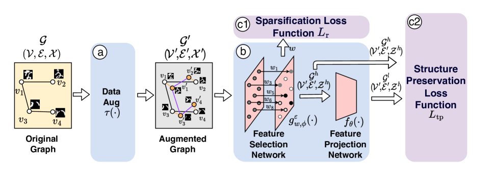
Figure 1: The framework of UDRN. The proposed UDRN consists of (a) data augmentation operation $\tau$, (b) feature selection (FS) network & feature projection (FP) network, (c) structure preservation loss function $L_{\text{tp}}$. The $\tau$ generates new augmented graph $\bm{\mathcal{G^{\prime}}}(\bm{\mathcal{V^{\prime}}},\bm{\mathcal{E^{\prime}}},\bm{\mathcal{X^{\prime}}})$ by Eq. (4). The FS network filter out unimportant features and map the data with selected features to high-dim embedding graph $\bm{\mathcal{G}^{h}}(\bm{\mathcal{V}^{\prime}},\bm{\mathcal{E}^{\prime}},\bm{\mathcal{Z}^{h}})$; FP network map the $\bm{\mathcal{G}^{h}}$ low-dim embedding graph $\bm{\mathcal{G}^{l}}(\bm{\mathcal{V}^{\prime}},\bm{\mathcal{E}^{\prime}},\bm{\mathcal{Z}^{l}})$. The $L_{\text{tp}}$ train FS and FP network with an end-to-end loss function.

The network framework of UDRN, the new manifold assumption and the proposed loss function are described in detail in this section. Moreover, the reasons for the performance improvement it brings are further analyzed.

4.1 UDRN Framework

As discussed in sec 3.2 to sec 3.4, current FS and FP methods are unable to meet the requirements of FS&FP task. Therefore, we propose a novel neural network framework to solve the FS&FP task. The framework of UDRN is shown in Fig. 1. The proposed UDRN contains a feature selection (FS) network $g_{\bm{w},\phi}^{\epsilon}(\cdot)$ and a feature projection (FP) network $f_{\bm{\phi}}(\cdot)$, each oriented to separate aim. The $g_{\bm{w},\phi}^{\epsilon}(\cdot)$ learn the sparse feature subset online and then map the data with selected features into high dimensional embedding $\bm{\mathcal{Z}}^{h}$, and then $f_{\bm{\phi}}(\cdot)$ further maps $\bm{\mathcal{Z}}^{h}$ to low dimensional embedding $\bm{\mathcal{Z}}^{l}$.

The forward propagation of feature selection (FS) network $g_{\bm{w},\phi}^{\epsilon}(\cdot)$ is,

$$\bm{\mathcal{Z}}^{h} =g_{\bm{w},\phi}^{\epsilon}(\bm{\mathcal{X^{\prime}}})=\text{m}_{\phi}\left(\text{GL}_{\bm{w}}^{\epsilon}\left(\bm{\mathcal{X^{\prime}}}\right)\right),$$ (13)

where the FS network includes a backbone network $\text{m}_{\phi}\left(\cdot\right)$ and a gate layer $\text{GL}_{\bm{w}}^{\epsilon}\left(\cdot\right)$. The $\phi$ is the network parameters of $\text{m}_{\phi}\left(\cdot\right)$. The gate layer $\text{GL}_{\bm{w}}^{\epsilon}\left(\cdot\right)$ processes the augmented data $\bm{\mathcal{X^{\prime}}}$ by a gate operation.

$$\text{GL}_{\bm{w}}^{\epsilon}(\bm{\mathcal{X^{\prime}}})=\left\{\begin{array}[]{cl}w_{j}\bm{\mathcal{X}_{j}^{\prime}}&\text{if }w_{j}>\epsilon,j\in\left\{1,2,\ldots,\mathcal{D}\right\}\\ 0&\text{otherwise}\end{array}\right.$$ (14)

where the $\bm{w}\in R^{\mathcal{D}}$ is gate parameters, indicating the importance of the features. The $\epsilon$ is a hyperparameter threshold, and the $g_{\bm{w},\phi}^{\epsilon}(\bm{\mathcal{X^{\prime}}})$ is a gate layer to ensure the features with low importance scores are not leakage to the latter network layer.

In this way, important features ($w_{j}>\epsilon$) can be passed through the gate layer and scaled by the gate parameters. And unimportant features will be blocked by the gate layer. The $\bm{w}$ is initialized to a constant value and is optimized according to the loss function of the network. Once $w_{j}<\epsilon$, the corresponding feature $j$ is discarded by the gate layer.

The forward propagation of the feature propagation (FP) network is,

$$\bm{\mathcal{Z}}^{l}=f_{\bm{\theta}}(\bm{\mathcal{Z}}^{h}).$$ (15)

The FP network $f_{\bm{\theta}}(\cdot)$ maps the h-dim embedding $\bm{\mathcal{Z}}^{h}$ to the $\bm{\mathcal{Z}}^{l}$ in l-dim for visulazation or other downstreem tasks. Finally, the outputs of UDRN are two graphs, which include the high dimensional embedding graph $\bm{\mathcal{G}}^{h}(\bm{\mathcal{V^{\prime}}},\bm{\mathcal{E^{\prime}}},\bm{\mathcal{Z}^{h}})$ and low dimensional embedding graph $\bm{\mathcal{G}}^{l}(\bm{\mathcal{V^{\prime}}},\bm{\mathcal{E^{\prime}}},\bm{\mathcal{Z}^{l}})$.

4.2 Manifold Connectivity Assumptions Under Augmented Data

Typical FS and FP methods are based on manifold assumptions [20, 63, 60, 64], which only focus on finite data in the dataset. These methods ignore estimating the intrinsic manifold from the finite and augmented data. It is a good choice to learn information about the intrinsic manifold by neural networks and to perform FS and FP based on the learned network parameters containing the information of the manifold.

To realize the above plan, the current manifold assumption has to be extended as it is not compatible with augmented data. As shown in Fig. 2, the typical DR loss does not take into account the augmented data, so the embedding of the latent space can only be learned based on the finite data. The ‘push’ and ‘pull’ are the figurative representation of the action of the loss function on the nodes of the latent space. Current typical methods cannot accommodate data augmentation. When additional augmented data is generated, the loss function of the current typical method causes an increase in computational complexity (because of the need to compute $\sigma^{*}$ for each augmented data) and model collapse (because of the inconsistency of the gradient caused by the data augmentation).

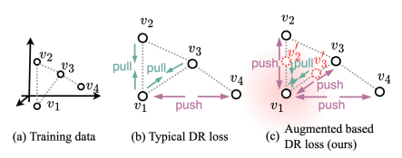
Figure 2: Manifold connectivity assumptions in data augmentation contexts. (a) High dimensional data used for training model. (b) Typical DR loss by ‘pushing and pulling’ the true sample to optimize the latent space. (c) The proposed DR method based on data augmentation generates new samples online and trains the model by ‘pushing and pulling’ augmented samples to learn the intrinsic manifold more precisely.

To this end, we propose a more stringent assumption, named manifold connectivity assumptions under augmented data. It assumes that the augmented data $\bm{x}^{{}^{\prime}}=\tau(\bm{x})$ is connected to the original data $x$ on the manifold. Based on this, the typical DR loss can be effectively expanded (as shown in Fig. 2). Instead of relying on the finite data in the dataset to optimize the neural network parameters, the proposed loss is combined with the augmented data to train the model. A sufficient prior embedded in the data augmentation allows the model to be trained without computing $\sigma^{*}$, which also avoids additional computational consumption. Also, the proposed assumptions can better avoid collapse and achieve more refined modeling.

4.3 Data Augmentation Compatible Loss Functions

Next, a novel loss function is designed to implement the assumptions proposed in Sec 4.2. The proposed loss function matches the network framework (in Sec 4.1) and data augmentation (Sec 3.3).

The proposed loss function first ensures the preservation of local information in the dimensionality reduction process by manifold exaggeration and then measures the difference between the latent space and the target with the fuzzy set cross entropy (in Fig. 3).

Figure 3: Framework of calculating $L_{\text{tp}}$. (1) abstract structure $\bm{\mathcal{E^{\prime}}}$. (2) use $\bm{\mathcal{E^{\prime}}}$ to exaggerate the high-dimensional NS $\mathcal{\bm{S}}^{\bm{h}}$. (3) calculate $L_{\text{tp}}$ by appling fuzzy set cross-entropy to $\mathcal{\bm{\tilde{S}}}^{\bm{h}}$ and $\mathcal{\bm{S}}^{\bm{l}}$.

The DR requires mapping high-dimensional data to a lower-dimensional space, which naturally brings about ‘crowding problem’. To alleviate the above ‘crowding problem’, pulling in neighboring nodes and pushing away non-neighboring nodes are good strategies. Because the above strategies can effectively avoid the manifold overlapping in the lower dimensional space. Thus we design manifold exaggeration,

$$\tilde{\bm{S}}_{ij}^{h} =E(\bm{S}_{ij}^{h},\bm{\mathcal{E^{\prime}}})$$ (16)

$$=\left\{\begin{aligned} &{\bm{S}}_{ij}^{h}\exp(1-\beta)&\text{ if }\left(\bm{v}_{i},\bm{v}_{j}\right)\in\bm{\mathcal{E^{\prime}}}&\\ &{\bm{S}}_{ij}^{h}\exp(1+\beta)&\text{otherwise}&\end{aligned}\right.$$

where the neighborhood relationship of augmented data $\bm{\mathcal{E^{\prime}}}$ is defined in Eq. (4). The $\bm{S}_{ij}^{h}$ is the node similarity, which is calculated from the nodes similarity in a high dimensional graph $\bm{\mathcal{G}^{h}}(\bm{\mathcal{V}^{\prime}},\bm{\mathcal{E}^{\prime}},\bm{\mathcal{Z}^{h}})$. $\bm{S}_{ij}^{h}=\kappa^{\text{Ga}}\left(\left\|\bm{z}_{i}^{h}-\bm{z}_{j}^{h}\right\|_{2}^{2},\sigma=1\right)$. The manifold exaggeration transforms the goal of network learning with neighbor relationship prior knowledge $\bm{\mathcal{E^{\prime}}}$, that is, increasing the goal similarity of neighboring nodes and decreasing the goal similarity of non-neighboring nodes. Thereby, the objective of pulling in neighbor nodes and pushing away non-neighbor nodes can be achieved. The hyperparameter $\beta>0$ controls the strength of exaggeration.

The loss function is designed as the form of fuzzy sets cross entropy [60] (two-way divergency in [65]),

$$L_{\text{tp}} =\frac{1}{B^{2}}\sum_{i,j\in\bm{\mathcal{B}}}\tilde{\bm{S}}_{ij}^{h}\log\bm{S}_{ij}^{l}+(1-\tilde{\bm{S}}_{ij}^{h})\log(1-\bm{S}_{ij}^{l})$$ (17)

where nodes similarity in a high dimensional graph is calculated as $\bm{S}_{ij}^{l}=\kappa^{\text{t}}\left(\left\|\bm{z}_{i}^{l}-\bm{z}_{j}^{l}\right\|_{2}^{2},\nu\right)$, $\nu$ is a hyperparameter. The $\bm{\mathcal{B}}=\{1,2,\ldots,B\}$, $B$ is the number of node in a batch. The loss function trains the neural network to output a low-dimensional embedding $z^{l}$ such that $\bm{S}_{ij}^{l}$ approximates the exaggerated $\tilde{\bm{S}}_{ij}^{h}$.

The designed loss function is based on the manifold connectivity assumption of augmented data and is well-compatible with data augmentation. As described in Sec. 4.3, it is assumed that the augmented data are neighbors of the original data in the real manifold. Therefore, instead of pulling in similar nodes in the dataset, the proposed loss function pulls in the augmented nodes. The online generation of augmented data during training allows the proposed method to depict the structure of the manifold in a more refined way, ultimately leading to performance improvements.

The designed loss function is consistent for FS and FP. We implement the selection of important features and the discarding of unimportant features in the forward propagation of the network with the help of the gate layer. And the whole selection process is embedded in the training of the neural network. The FS and FP are based on the same object, which is to better preserve the structure of neighbors in higher dimensional spaces in a lower dimensional space.

Finally, the loss function of unsupervised UDRN is:

$$\min_{w,\bm{\theta},{\bm{\phi}}}\ \ L_{\text{tp}}+\lambda L_{\text{r}},\ \ \ \ L_{\text{r}}=\|\bm{w}\|_{1},$$ (18)

where $\lambda$ is hyperparameter. To select a specific feature number, we give $\lambda$ a small initial value, and then slowly increase $\lambda$ until the feature number satisfies the requirements.

4.4 Pseudocode

Algorithm. 1 shows how to train our model and how to obtain the selected features.

Algorithm 1 The UDRN algorithm

Input: Data: $\bm{\mathcal{G}_{\text{all}}}(\bm{\mathcal{V}},\bm{\mathcal{E}},\bm{\mathcal{X}})$, Learning rate: $\alpha$, Epochs: $E$, Batch size: $B$, Network: $g_{w,\theta}^{\epsilon},f_{\theta}$, loss weights: $\lambda$,
Output: Selected Features: $\bm{\mathcal{X}}^{h}$. FS&FP Embedding: $\bm{\mathcal{Z}_{\text{all}}^{l}}$.

1:  Let $t=0$.

2:  while $i=0$; $i<E$; $i$++ do

3:     while $b=0$; $b<[|\mathcal{X}|/B]$; $b$++ do

4:        $\bm{\mathcal{G}}(\bm{\mathcal{V}},\bm{\mathcal{E}},\bm{\mathcal{X}})$ $\leftarrow$ Sampling($\bm{\mathcal{G}_{\text{all}}}(\bm{\mathcal{V}},\bm{\mathcal{E}},\bm{\mathcal{X}})$, b); # Sample a batch data

5:        $\bm{\mathcal{G}}^{\prime}(\bm{\mathcal{V}}^{\prime},\bm{\mathcal{E}}^{\prime},\bm{\mathcal{X}}^{\prime})$ $\leftarrow$ Augment($\bm{\mathcal{G}}(\bm{\mathcal{V}},\bm{\mathcal{E}},\bm{\mathcal{X}})$) by Eq. (4); # Data augmentation

6:        $\bm{\mathcal{X}}^{h}=m(\bm{\mathcal{X^{\prime}}})$ by Eq. (13); # Select the features

7:        $\bm{\mathcal{G}^{h}}(\bm{\mathcal{V}^{\prime}},\bm{\mathcal{E}^{\prime}},\bm{\mathcal{Z}^{h}})$ $\leftarrow$ $g(\bm{\mathcal{G^{\prime}}}(\bm{\mathcal{V^{\prime}}},\bm{\mathcal{E^{\prime}}},\bm{\mathcal{X}}^{h}))$ by Eq. (13); # Map to high dimension space

8:        $\bm{\mathcal{G}^{l}}(\bm{\mathcal{V}^{\prime}},\bm{\mathcal{E}^{\prime}},\bm{\mathcal{Z}^{l}})$ $\leftarrow$ $f(\bm{\mathcal{G}^{h}}(\bm{\mathcal{V}^{\prime}},\bm{\mathcal{E}^{\prime}},\bm{\mathcal{Z}^{h}}))$ by Eq. (15); # Map to low dimension space

9:        $\bm{S}_{ij}^{h}$ $\leftarrow$ $S(\bm{\mathcal{G}^{h}}(\bm{\mathcal{V}^{\prime}},\bm{\mathcal{E}^{\prime}},\bm{\mathcal{Z}^{h}}))$; # Cal high dim similarity

10:        $\bm{S}_{ij}^{l}$ $\leftarrow$ $S(\bm{\mathcal{G}^{l}}(\bm{\mathcal{V}^{\prime}},\bm{\mathcal{E}^{\prime}},\bm{\mathcal{Z}^{l}}))$; # Cal low dim similarity

11:        $\tilde{\bm{S}}_{ij}^{h}$ $\leftarrow$ $E(\bm{S}_{ij}^{h},\bm{\mathcal{E^{\prime}}})$; # Manifold exaggeration

12:        $\mathcal{L}_{\text{tp}}\!\leftarrow\!L_{\text{tp}}(\tilde{\bm{S}}_{ij}^{h},\bm{S}_{ij}^{l})$ by Eq. (17); # Cal. the structural preservation loss

13:        $\mathcal{L}_{\text{1}}\!\leftarrow\!L_{\text{1}}(\bm{w})$ by Eq. (18); # Cal. the L1 loss

14:        $\theta,\!\leftarrow\!\theta-\alpha\frac{\partial\mathcal{L}_{\text{tp}}}{\partial\theta}$, $\phi\!\leftarrow\!\phi-\alpha\frac{\partial\mathcal{L}_{\text{tp}}}{\partial\phi}$, $\bm{w}\!\leftarrow\!\bm{w}-\alpha(\frac{\partial\mathcal{L}_{\text{tp}}}{\partial\bm{w}}+\frac{\partial\mathcal{L}_{\text{1}}}{\partial\bm{w}})$ # Update the parameters

15:     end while

16:  end while

17:  $\bm{\mathcal{X}}^{h}\leftarrow m(\bm{\mathcal{G}_{\text{all}}}(\bm{\mathcal{V}},\bm{\mathcal{E}},\bm{\mathcal{X}}))$; # Select the features

18:  $\bm{\mathcal{G}^{l}_{\text{all}}}(\bm{\mathcal{V}_{\text{all}}^{\prime}},\bm{\mathcal{E}_{\text{all}}^{\prime}},\bm{\mathcal{Z}_{\text{all}}^{l}})\leftarrow f(g(\bm{\mathcal{G}_{\text{all}}}(\bm{\mathcal{V}},\bm{\mathcal{E}},\bm{\mathcal{X}})))$; # Cal. the embedding result

5 Experiments

5.1 Details of Dataset and Compared Methods

Details of Dataset. We used four image datasets (COIL20, Mnist, KMnist, EMnist) and four biological datasets (Activity, HCL, Gast, and MCA). The details of the dataset are shown in Table 1. Unlike CAE [17] and FAE [18], we do not downsample the dataset because of the computational time. We consider performance on large datasets as an essential evaluation metric.

Table 1: Statistics of datasets.

	Dataset	#Sample	#Feature	#Class	Link
Image Data	Coil20	1440	16384	20	https://www.cs.columbia.edu/CAVE/ software/softlib/coil-20.php
	KMnist	60,000	784	10	https://pytorch.org/vision/stable/index.html
	Mnist	60,000	784	10	https://pytorch.org/vision/stable/index.html
	EMnist	731,668	784	10	https://pytorch.org/vision/stable/index.html
Biological Data	Activity	5,744	561	6	https://www.kaggle.com/uciml/human-activity-recognition-with-smartphones
	GAST	10,629	1457	12	https://www.ncbi.nlm.nih.gov/pmc/articles/PMC4643992/
	MCA	30,000	9119	52	http://bis.zju.edu.cn/MCA/
	HCL	280,000	3037	93	https://figshare.com/articles/dataset/ HCL_DGE_Data/7235471

Compared Methods. To demonstrate the advantages of UDRN, we compare it with the FS methods, the FP methods, and the pipeline methods of FS and FP. The compared methods are divided into non-parameters methods and parameters methods. The non-parameters FS methods include LS [25], MCFS [66], NDFS [67], and IVFS [16]. The compared parameters FS methods include AEFS [30], CAE [17], FAE [55], and QS [33]. The compared non-parameters FP methods include tSNE [68], UMAP [41]. The compared parameters FP methods include GRAE [69], IVIS [70] and Parametric UMAP (PUMAP) [71].

The grid search is used to determine the optimal parameters for all the baseline methods. The search space of each method is shown in Table. 2.

Table 2: Details of grid search.

Methods	Search Space	Note
LS	$C\in[5,10,15,20,25,30,35,40,45,50]$	$C\to\text{cluster range}$
MCFS	$C\in[5,10,15,20,25,30,35,40,45,50]$	$C\to\text{cluster range}$
NDFS	$A\in[1,1.5,2]$,$BETA\in[0.5,1,2]$,$C\in[5,15,25]$	$A\to\alpha$, $C\to\text{cluster range}$
IVFS	$T\in[D//10,D//20,D//50,D//80]$	$T\to\text{tilde sample range},D\to\text{data shape}$
AEFS	$A\in[0.1,0.2,0.5]$, $E\in[500,1000,2000]$	$A\to\alpha,E\to\text{epoch}$
CAE	$B\in[256,512]$, $LR\in[0.01,0.1,1]$, $DR\in[0,0.5,0.8]$	$B\to\text{batch},LR\to\text{learning rate},DR\to\text{dropout}$
FAE	$B\in[128,256,512]$,$E\in[500,1000,2000]$	$B\to\text{batch}$, $E\to\text{epoch}$
QS	$EP\in[2,5,10,13,20,25]$,$Z\in[0.1,0.2,0.3,0.4,0.5]$	$EP\to\epsilon$, $Z\to\zeta$

5.2 Experimental Setup

We initialize the weights of the FS layer to $\bm{w}=0.2$ and initialize the other NN with the Kaiming initializer. We adopt the AdamW optimizer [72] with a learning rate of 0.001. All experiments use a fixed MLP network structure, $g_{\bm{w}}^{\epsilon}$: [-1, 500, 300, 80], $f_{\theta}$: [80, 500, 2], where -1 is the features number of the dataset, the first layer of $g_{\bm{w}}^{\epsilon}$ is the gate layer. To make UDRN select a specified number of features, we set an adaptive $\lambda$. At the beginning of 300 epochs, the $\lambda=0$ model, and then $\lambda=L_{\text{r}}/0.1\|\bm{w}\|_{1}$ and grow by 0.5% until the number of features meet the requirements. For all experiments $\beta=0.01$. For the experiments in Table 3 to Table 6, we used Bernoulli-type FMH augmentation and set $p_{N}=0.3$. For a fair comparison, the training set (80% data) is used for the model training and feature selection; the validation set (10%) is used to select the best hyperparameters with grid search; the performance on the test set (10%) is reported in this paper.

Table 3: Discriminative performance (classification accuracy) comparison with FS methods in image datasets; best result are shown in blod; results with clear advantage are shown in underline.

	LS	MCFS	NDFS	IVFS	AEFS	CAE	FAE	QS	UDRN
Coil20	21.0$\pm$0.6	34.0$\pm$1.3	8.1$\pm$1.5	98.6$\pm$0.7	99.3$\pm$0.2	97.7$\pm$0.7	84.1$\pm$0.2	98.0$\pm$0.5	99.4$\pm$0.2($\uparrow$0.1)
MNIST	17.0$\pm$0.1	76.0$\pm$0.4	90.4$\pm$0.6	42.4$\pm$0.1	86.4$\pm$0.3	92.1$\pm$0.2	70.5$\pm$0.4	93.2$\pm$0.2	94.3$\pm$0.3($\uparrow$1.1)
KMNIST	20.1$\pm$0.2	64.0$\pm$0.5	83.9$\pm$0.3	82.4$\pm$0.5	85.6$\pm$0.4	88.0$\pm$0.3	77.6$\pm$0.2	85.9$\pm$0.3	90.7$\pm$0.4($\uparrow$2.7)
EMNIST	7.9$\pm$0.1	43.6$\pm$0.9	64.3$\pm$0.6	42.5$\pm$0.3	65.6$\pm$0.4	63.9$\pm$0.3	52.0$\pm$0.3	68.0$\pm$0.3	71.1$\pm$0.5($\uparrow$3.1)
Average	16.5$\pm$0.2	54.4$\pm$0.6	61.7$\pm$0.8	66.5$\pm$0.5	84.2$\pm$0.3	85.4$\pm$0.4	64.8$\pm$0.3	86.2$\pm$0.3	88.9$\pm$0.4($\uparrow$2.7)

Table 4: Discriminative performance (classification accuracy) comparison with FS methods in biology datasets, best result are shown in blod; results with clear advantage are shown in underline.

	LS	MCFS	NDFS	IVFS	AEFS	CAE	FAE	QS	UDRN
Activity	92.3$\pm$0.3	42.4$\pm$1.8	48.5$\pm$3.8	95.8$\pm$0.3	96.9$\pm$0.2	98.0$\pm$0.1	74.8$\pm$0.8	97.4$\pm$0.2	98.6$\pm$0.3($\uparrow$0.6)
HCL	23.6$\pm$0.2	7.2 $\pm$0.5	09.2$\pm$0.2	21.8$\pm$0.2	24.7$\pm$0.2	28.5$\pm$0.1	33.0$\pm$0.2	56.7$\pm$0.3	58.9$\pm$0.2($\uparrow$2.2)
Gast	68.9$\pm$0.5	42.1$\pm$3.6	44.4$\pm$1.6	73.9$\pm$0.6	73.6$\pm$0.6	89.1$\pm$0.3	81.0$\pm$0.3	86.8$\pm$0.6	90.0$\pm$0.4($\uparrow$0.9)
MCA	19.5$\pm$0.2	24.5$\pm$0.1	56.8$\pm$0.6	27.0$\pm$0.1	28.6$\pm$0.2	66.8$\pm$0.2	32.8$\pm$0.2	64.3$\pm$0.4	77.8$\pm$0.4($\uparrow$11.0)
Average	42.4$\pm$0.3	31.9$\pm$1.2	44.6$\pm$1.4	52.2$\pm$0.3	57.8$\pm$0.3	69.2$\pm$0.2	54.3$\pm$0.4	74.6$\pm$0.3	81.3$\pm$0.3($\uparrow$6.7)

5.3 Case Study

Figure 4: Case Study. (a) Variation plot of feature importance during training. Curves show the change in feature importance. colored curves (final selected features); gray curves (final discarded features). (b) Variation plot of the number of essential features ($w_{f}>\epsilon$) and loss function weights $\lambda$ during training. (c) UMAP Visualization of all features and the selected features. The color of the points in the scatter plot marks the true label of the data.

The Mnist dataset is selected to illustrate how UDRN works (Fig. 4). The FS processing. At the beginning of training, we set $\bm{w}=0.2$. The gate layer passes all features in the dataset. With the training going on, the $L_{\text{r}}$ loss reduces $\bm{w}$ and $L_{\text{tp}}$ loss increases $\bm{w}$. Eventually, only features that are important for structure preservation can pass the gate layer. The unimportant features are discarded (as shown in Fig. 4 (a) and Fig. 4 (b)).

FS & structure-preservation. We expect the FS of UDRN to affect the local and global structure of the data as little as possible, which is the original intention of using the unified loss function for both FS and FP tasks. We find that humans can easily recognize numbers in images based on selected features, indicating that our FS does not destroy the discriminative nature of the images (in Fig. 4(c)). To further confirm this, UMAP is used to process the pre-FS data and post-FS data. The results (in Fig. 4(c)) show that the clustering relationship of the data is found not to be changed by FS.

5.4 Comparison with FS methods

This sub-section compares the performance with the unsupervised FS methods. The performance comparison includes discriminative performance and structure-preservation performance.

Discriminative performance. The discriminative performance shows the ability of the features selected by the FS method in the classification task. Following CAE [17] and FAE [55], the discriminative performance is measured by passing the selected features to a downstream classifier (Extremely Randomized Trees classifier, a variant of Random Forest) as a viable means to benchmark the quality of the selected subset of features.

For all methods, we select 64 features as benchmarks. The means and standard deviations of the accuracy are shown in Table. 3 and Table. 4. For a more extensive comparison, we compare the cases of selecting [16, 32, 64, 128, 256, 512] features. The comparison results are shown in Fig. 5.

Analysis. The conclusions are as follows. (a) In general, parametric methods are superior to other methods. Among the parametric methods, UDRN has the best results. UDRN has an advantage in all nine datasets. In addition, UDRN outperformed the second-best method by 1% in six datasets. (b) UDRN has more advantages in data with more features; for example, in data sets with more than 1000 features (in Table. 4), UDRN has more obvious advantages.

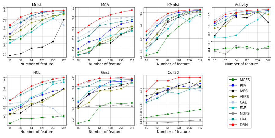
Figure 5: Classification accuracy with the number of selected features. The horizontal coordinate represents the number of selected features, and the vertical coordinate is the ACC of classification.

Structure-preservation performance. The structure-preservation performance tests whether the FS methods preserve the neighborhood relationship of the original data. The structure matching degree (SMD), a sampling-based structure metric, is chosen as an evaluation metric.

$$\text{SMD}=\frac{1}{k|\mathcal{\bm{V}}|}\sum_{i\in\bm{\mathcal{X}},j\in\mathcal{N}^{k}(i)}\left|r_{i,j}^{\mathcal{\bm{X}}}-r_{i,j}^{\mathcal{\bm{X}}^{h}}\right|$$ (19)

where the $r_{i,j}^{\mathcal{\bm{X}}}$ and $r_{i,j}^{\mathcal{\bm{X}}^{s}}$ are the neighborhood ranking of $\bm{v}_{j}$ in $\bm{v}_{i}$ in the input and latent space. The results of the datasets are shown in Table 5.

Analysis. The conclusions are as follows. (a) Parametric methods, except UDRN, concentrate on reconstructing all the input features and do not preserve the structure of the selected features well. (b) Many non-parametric methods design objective functions based on structure retention and achieve suboptimal performance. (c) UDRN achieves the best score, which is attributed to the fact that the data augmentation of UDRN and the accompanying loss function learn a finer manifold structure.

Table 5: Structure-preserving performance (SMD) comparison, best results are shown in blod.

	LS	IVFS	AEFS	CAE	FAE	UDRN
Coil20	12.0	83.2	52.5	41.5	67.8	86.3
Mnist	17.0	86.9	59.6	42.7	46.8	89.9
KMnist	27.6	86.9	63.2	61.4	49.5	88.3
EMnist	31.8	69.1	71.2	75.9	65.5	79.8
Activity	43.1	81.9	50.5	44.7	53.5	99.9
HCL	11.9	22.1	11.5	10.4	13.6	27.8
Gast	35.2	39.0	27.0	15.8	31.2	48.2
MCA	16.5	21.0	16.7	13.7	16.6	26.9

5.5 Comparison with FP methods

This sub-section compares the performance with the baseline FP methods.

For a fair comparison with FP methods, we disable the gate layer by setting $\lambda=0$, these means that all the features can pass the gate layer. Similar to sec. 5.4, we evaluate the discriminative performance by the accuracy of the ET tree classifier. The other settings are the same as sec. 5.4. The comparison results are shown in Table 6.

Analysis. The conclusions are as follows. (a) Except for UDRN, the performance of parametric methods is inferior to that of non-parametric methods. UDRN is not only optimal among all parametric methods but also superior to non-parametric methods. The results are consistent with those in [14]. (b) The parametric FP methods are challenging to train because the network parameters need to be optimized rather than the low-dimensional representations. Interestingly, UDRN can solve the training problem of FP networks through data augmentation and novel loss functions.

Table 6: Discriminative performance comparison with FP methods, best results are shown in blod.

	tSNE	UMAP	GRAE	IVIS	PUMAP	UDRN
Coil20	78.1	79.6	79.9	58.9	68.9	89.8
MNIST	95.9	94.5	77.2	68.3	94.2	95.9
KMNIST	64.3	93.8	85.4	72.8	91.5	94.7
EMNIST	72.2	74.7	72.4	36.7	77.5	73.5
Activity	92.0	91.9	88.9	82.1	90.0	92.6
HCL	58.4	44.9	53.1	53.3	51.4	91.7
Gast	69.5	62.7	90.1	76.4	64.5	94.8
MCA	51.5	41.3	83.6	66.7	46.6	90.9

5.6 Visualization Comparison with FS&FP Pipeline

In application areas such as biology, many articles require a combination of FP and FS methods for data analysis because of the high data dimensionality and excessive noise features [73, 19]. We have discussed the dilemma of these methods in sec 2. Since the concept of unifying FP&FS is first proposed by us, these pipeline methods are compared in this article. In Fig. (6), the advantages of UDRN are demonstrated by visualization. The FP method (UMAP) and FS methods (IVFS, CAE, and QS), which performed best in sec.5.4 and sec.5.5, are selected as the elements of the pipeline.

Analysis. The conclusions are as follows. (a) When using all features, UMAP and UDRN can clearly show the structure, although different in detail. (b) When selecting fewer features, the compared methods can not guarantee the stability of the data’s structure. For example, the embedding of features selected by IVFS differs from the embedding of the original features. (c) UDRN is very good at producing stable embeddings with only a small number of features due to the uniform loss function and data augmentation. The UDRN performs significantly better than the pipeline method from the visualization point of view.

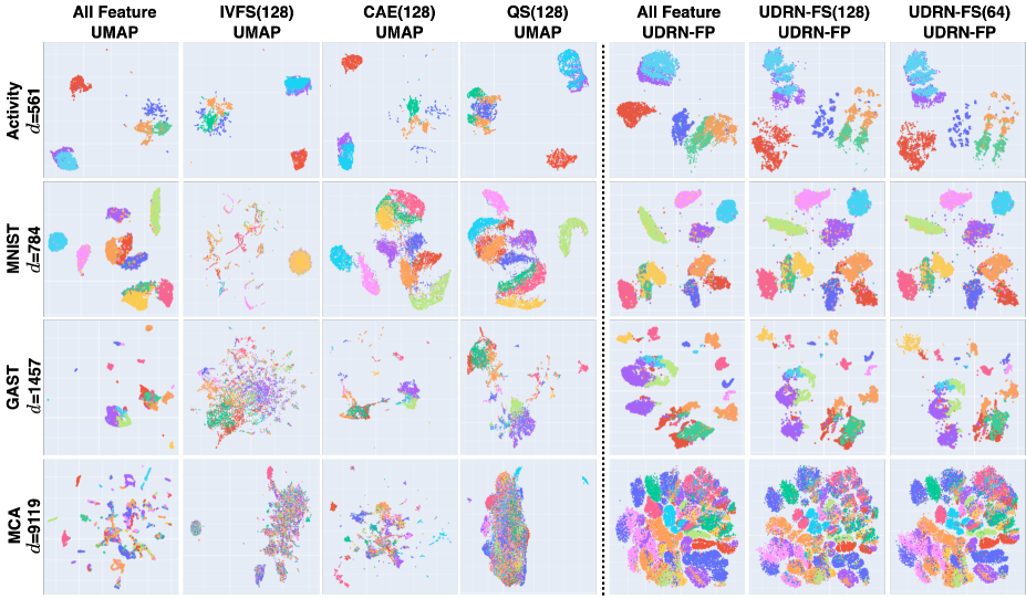
Figure 6: Visualization comparison with FS&FP pipeline. Each row corresponds to a dataset. In the row names, $D$ represents the number of features in the dataset. Each column corresponds to a combination of FS and FP methods. In the column names, the first occurrence of the feature selection method, the number of selected features is in parentheses, and the second occurrence is the feature mapping method. To align with the baseline nomenclature, our UDRNs are divided into UDRN-FS and UDRN-FP. The parentheses after UDRN-FS are used to indicate the number of selected features.

5.7 Parameter Analysis

Table 7: Ablation study. The discriminative performance comparison on the training set with different data augmentation hyperparameters. $0.0$ means without the data augmentation.

Uniform-type Data Aaugmentation, $\tau_{U}(\cdot)$
$p_{U}$	0.0	0.03	0.05	0.08	0.10	0.30	0.50
Mnist	91.5	92.0	93.3	93.0	92.8	93.5	93.0
KMnist	84.2	88.1	87.9	89.5	87.6	88.6	85.7
EMnist	64.7	67.5	69.8	69.5	70.6	69.7	69.4
HCL	45.2	58.8	60.1	57.1	61.0	57.8	63.0
MCA	45.5	70.8	70.3	61.5	60.5	50.4	60.0
Gast	72.0	88.4	87.6	90.3	89.3	90.0	89.4
AVE	68.1	78.0	78.2	77.2	77.3	75.3	77.6
Bernoulli-type Data Aaugmentation, $\tau_{B}(\cdot)$
$p_{{B}}$	0.0	0.03	0.05	0.08	0.10	0.30	0.50
Mnist	91.5	93.6	94.6	94.2	94.1	94.0	94.0
KMnist	84.2	89.7	89.7	89.7	89.9	89.7	89.9
EMnist	64.7	71.3	71.0	71.4	70.9	70.4	70.2
HCL	44.2	63.0	62.8	62.6	63.3	62.4	59.8
MCA	45.5	52.4	59.6	56.8	53.6	51.4	61.7
Gast	72.0	89.4	89.9	89.6	89.1	89.2	88.2
AVE	68.1	77.4	77.8	78.4	77.9	77.0	78.0
Normal-type Data Aaugmentation, $\tau_{N}(\cdot)$
$p_{N}$	0.0	0.03	0.05	0.08	0.10	0.30	0.50
Mnist	91.5	93.8	94.1	93.8	94.6	94.3	94.2
KMnist	84.2	85.6	89.7	90.3	89.9	90.7	90.0
EMnist	64.5	65.9	69.8	69.6	70.5	71.4	71.4
HCL	47.1	56.3	56.9	57.7	59.8	58.9	59.4
MCA	45.5	71.5	72.2	75.3	74.9	73.3	73.4
Gast	72.0	86.7	86.9	87.4	88.5	90.0	89.8
AVE	68.1	77.9	78.2	78.4	79.7	80.1	79.4

In this sub-section, the effect of hyperparameters of data augmentation is analyzed and the stability of the hyperparameters is discussed. We follow the sec. 5.4’s setup and tested on the Mnist, EMnist, KMnist, HCL, MCA, and Gast datasets. The average ACC is shown in Table. 7.

Analysis. The conclusions are as follows. (1) FMH augmentation significantly enhances UDRN. Using any data augmentations can dramatically improve the method’s performance. (2) The parameters of data augmentation have a relatively small impact on the algorithm, and in short, Normal-type FMH has a relative advantage. In general, the parameters of the FMH augmentation are very stable.

5.8 Ablation Study

In this sub-section, the effect of innovations of UDRN is analyzed by ablation experiments. We follow the sec. 5.4’s setup and tested on the Mnist, KMnist, EMnist, HCL, and MCA datasets. The discriminative and the structure-preserving performance is shown in Table 8 and Table 9. Ablation 1 (w/o $\tau$). First, the data augmentation $\tau$ is removed. The model is trained directly using the original data $\bm{\mathcal{G}}(\bm{\mathcal{V}},\bm{\mathcal{E}},\bm{\mathcal{X}})$. Ablation 2 (w/o $L_{\text{tp}}$). Second, the proposed loss function $L_{\text{tp}}$ is removed and replaced with $L_{\text{FP}}$. Ablation 3 (w/o $\tau$&$L_{\text{tp}}$). Finally, both data augmentation $\tau$ and the proposed loss function $L_{\text{tp}}$ are removed.

Analysis. The conclusions are as follows. (1) Both of the innovations presented in this paper lead to performance improvements. And both can work with each other to achieve better performance. (2) Directly using the reconstructed loss function $L_{\text{FP}}$ instead of the proposed loss function reduces the performance of the model. It includes both discriminative and structure-preserving performance. Among them, the impact on the structure preservation performance is more significant.

Table 8: Ablation study of UDRN. The discriminative performance comparison under different ablation settings.

	Mnist	KMnist	EMnist	HCL	MCA
UDRN	94.3	90.7	71.1	58.9	77.8
w/o $\tau$	91.5	84.2	64.7	44.2	45.5
w/o $L_{\text{tp}}$	87.3	85.2	63.3	35.8	56.2
w/o $\tau$&$L_{\text{tp}}$	82.5	82.3	61.8	31.6	42.1

Table 9: Ablation study of UDRN. The structure-preserving performance comparison under different ablation settings.

	Mnist	KMnist	EMnist	HCL	MCA
UDRN	89.9	88.3	79.8	27.8	26.9
w/o $\tau$	85.3	86.2	74.3	25.5	22.7
w/o $L_{\text{tp}}$	35.3	39.2	25.8	15.5	17.5
w/o $\tau$&$L_{\text{tp}}$	36.2	34.8	26.4	17.4	12.1

5.9 Supervised UDRN (S-UDRN)

UDRN is well compatible with both supervised and unsupervised cases and only needs to consider whether supervised information is available when constructing the graph structure (in Eq. (1) and Eq. (2)). We chose a gut flora dataset to test UDRN under supervised scenarios. Since the gut flora dataset has few features associated with the labels, UDRN is needed to select highly relevant features from all the labels and complete the FP (in Fig. 7).

Analysis. (a) The dataset contains many useless features such that the unsupervised scheme is unable to distinguish classes. (b) Our UDRN approach can learn to distinguish labeled features based on a modified graph structure (based on labels), while at the same time, the intra-class manifold structure embedding does not receive influence.

Figure 7: Visualization of unsupervised UDRN (UDRN) and supervised UDRN (S-UDRN). The proposed UDRN method is also compatible with the supervised case and performs FS&FP based on data labels or other prior knowledge.

6 Conclusion

We developed an integrated method for feature selection (FS) and feature projection (FP) with the help of neural networks named Unified Dimensional Reduction Neural-networks (UDRN). UDRN handles FS and FP tasks end-to-end with a unified loss function. UDRN is compatible with both supervised and unsupervised settings. We demonstrate the effectiveness and sophistication of UDRN by working with state-of-the-art FS, FP, and FS&FP pipeline methods.

References

- Ayesha et al. [2020] S. Ayesha, M. K. Hanif, R. Talib, Overview and comparative study of dimensionality reduction techniques for high dimensional data, Information Fusion 59 (2020) 44–58.
- Li et al. [2020] S. Z. Li, Z. Zang, L. Wu, Deep manifold transformation for dimension reduction, arXiv (2020).
- Zang et al. [2022] Z. Zang, S. Cheng, L. Lu, H. Xia, L. Li, Y. Sun, Y. Xu, L. Shang, B. Sun, S. Z. Li, Evnet: An explainable deep network for dimension reduction, IEEE Transactions on Visualization and Computer Graphics (2022) 1–18.
- Chen et al. [2013] B. Chen, L. Chen, Y. Chen, Efficient ant colony optimization for image feature selection, Signal processing 93 (2013) 1566–1576.
- Liu et al. [2018] Z.-T. Liu, M. Wu, W.-H. Cao, J.-W. Mao, J.-P. Xu, G.-Z. Tan, Speech emotion recognition based on feature selection and extreme learning machine decision tree, Neurocomputing 273 (2018) 271–280.
- Deraeve and Alexander [2018] J. Deraeve, W. H. Alexander, Fast, accurate, and stable feature selection using neural networks, Neuroinformatics 16 (2018) 253–268.
- Remeseiro and Bolon-Canedo [2019] B. Remeseiro, V. Bolon-Canedo, A review of feature selection methods in medical applications, Computers in biology and medicine 112 (2019) 103375.
- Van Der Maaten et al. [2009] L. Van Der Maaten, E. Postma, J. Van den Herik, et al., Dimensionality reduction: a comparative, J Mach Learn Res 10 (2009) 13.
- Wang [2021] L. Wang, Single-cell normalization and association testing unifying crispr screen and gene co-expression analyses with normalisr, Nature communications 12 (2021) 1–13.
- Sheng and Li [2021] J. Sheng, W. V. Li, Selecting gene features for unsupervised analysis of single-cell gene expression data, Briefings in bioinformatics 22 (2021) bbab295.
- Zhang et al. [2021] Z. Zhang, F. Cui, C. Lin, L. Zhao, C. Wang, Q. Zou, Critical downstream analysis steps for single-cell rna sequencing data, Briefings in Bioinformatics 22 (2021) bbab105.
- Jiang et al. [2022] R. Jiang, T. Sun, D. Song, J. J. Li, Statistics or biology: the zero-inflation controversy about scrna-seq data, Genome biology 23 (2022) 1–24.
- Sun et al. [2022] Y. Sun, S. Selvarajan, Z. Zang, W. Liu, Y. Zhu, H. Zhang, W. Chen, H. Chen, L. Li, X. Cai, et al., Artificial intelligence defines protein-based classification of thyroid nodules, Cell discovery 8 (2022) 1–17.
- Xia et al. [2021] J. Xia, Y. Zhang, J. Song, Y. Chen, Y. Wang, S. Liu, Revisiting dimensionality reduction techniques for visual cluster analysis: An empirical study, IEEE Transactions on Visualization and Computer Graphics (2021) 1.
- Wei et al. [2016] X. Wei, B. Cao, S. Y. Philip, Unsupervised feature selection on networks: a generative view, in: Thirtieth AAAI Conference on Artificial Intelligence, 2016, pp. 1–48.
- Li et al. [2020] X. Li, C. Wu, P. Li, Ivfs: Simple and efficient feature selection for high dimensional topology preservation, national conference on artificial intelligence (2020) 103.
- Abid et al. [2020] A. Abid, M. F. Balin, J. Zou, Concrete autoencoders: Differentiable feature selection and reconstruction, in: ICML, Long Beach, California, United States, 2020, pp. 444–453.
- Wu and Cheng [2022] X. Wu, Q. Cheng, Fractal autoencoders for feature selection, in: National Conference on Artificial Intelligence, 2022, pp. 831–842.
- Townes et al. [2019] F. W. Townes, S. C. Hicks, M. J. Aryee, R. A. Irizarry, Feature selection and dimension reduction for single-cell rna-seq based on a multinomial model, Genome biology 20 (2019) 1–16.
- Lin and Zha [2008] T. Lin, H. Zha, Riemannian manifold learning, IEEE transactions on pattern analysis and machine intelligence 30 (2008) 796–809.
- McInnes et al. [2018] L. McInnes, J. Healy, J. Melville, UMAP: Uniform Manifold Approximation and Projection for Dimension Reduction, arXiv:1802.03426 [cs, stat] (2018). ArXiv: 1802.03426 version: 1.
- Alelyani et al. [2018] S. Alelyani, J. Tang, H. Liu, Feature selection for clustering: A review, Data Clustering (2018) 29–60.
- Peng et al. [2017] C. Peng, Z. Kang, Y. Hu, J. Cheng, Q. Cheng, Nonnegative matrix factorization with integrated graph and feature learning, ACM Transactions on Intelligent Systems and Technology (TIST) 8 (2017) 1–29.
- da Costa et al. [2021] N. L. da Costa, M. D. de Lima, R. M. Barbosa, Evaluation of feature selection methods based on artificial neural network weights, Expert Systems With Applications (2021).
- He et al. [2006] X. He, D. Cai, P. Niyogi, Laplacian score for feature selection, in: NeuIPS, 2006, pp. 507–514.
- Lu et al. [2007] Y. Lu, I. Cohen, X. S. Zhou, Q. Tian, Feature selection using principal feature analysis, in: 15th ACM international conference on Multimedia, 2007, pp. 301–304.
- Cai et al. [2010] D. Cai, C. Zhang, X. He, Unsupervised feature selection for multi-cluster data, in: SIGKDD, 2010, pp. 333–342.
- Yang et al. [2011] Y. Yang, H. T. Shen, Z. Ma, Z. Huang, X. Zhou, L2, 1-norm regularized discriminative feature selection for unsupervised, in: Twenty-Second International Joint Conference on Artificial Intelligence, 2011, p. 103.
- Li et al. [2012] Z. Li, Y. Yang, J. Liu, X. Zhou, H. Lu, Unsupervised feature selection using nonnegative spectral analysis, in: AAAI, volume 26, 2012, p. 103.
- Han et al. [2018] K. Han, Y. Wang, C. Zhang, C. Li, C. Xu, Autoencoder inspired unsupervised feature selection, in: International Conference on Acoustics, Speech and Signal Processing, Calgary, Alberta, Canada, 2018, pp. 2941–2945.
- Doquet and Sebag [2019] G. Doquet, M. Sebag, Agnostic feature selection, in: Joint European Conference on Machine Learning and Knowledge Discovery in Databases, Würzburg, Germany, 2019, pp. 343–358.
- Maddison et al. [2017] C. J. Maddison, A. Mnih, Y. W. Teh, The concrete distribution: A continuous relaxation of discrete random variables, arXiv: 1611.00712v3, https://arxiv.org/abs/1611.00712 (2017).
- Ata. et al. [2022] Z. Ata., G. Sokar, T. van der Lee, E. Mocanu, D. C. Mocanu, R. Veldhuis, M. Pechenizkiy, Quick and robust feature selection: the strength of energy-efficient sparse training for autoencoders, Machine Learning (2022) 1–38.
- Belkin and Niyogi [2003] M. Belkin, P. Niyogi, Laplacian eigenmaps for dimensionality reduction and data representation, Neural computation 15 (2003) 1373–1396.
- Fefferman et al. [2016] C. Fefferman, S. Mitter, H. Narayanan, Testing the manifold hypothesis, Journal of American Mathematical Society 29 (2016) 983–1049.
- Tenenbaum et al. [2000] J. B. Tenenbaum, V. De Silva, J. C. Langford, A global geometric framework for nonlinear dimensionality reduction, science 290 (2000) 2319–2323.
- Roweis and Saul [2000] S. T. Roweis, L. K. Saul, Nonlinear dimensionality reduction by locally linear embedding, science 290 (2000) 2323–2326.
- Donoho and Grimes [2003] D. L. Donoho, C. Grimes, Hessian eigenmaps: Locally linear embedding techniques for high-dimensional data, Proceedings of the National Academy of Sciences 100 (2003) 5591–5596.
- Zhang and Wang [2007] Z. Zhang, J. Wang, Mlle: Modified locally linear embedding using multiple weights, in: Advances in Neural Information Processing systems, 2007, pp. 1593–1600.
- Maaten and Hinton [2008] L. v. d. Maaten, G. Hinton, Visualizing data using t-sne, Journal of machine learning research 9 (2008) 2579–2605.
- McInnes et al. [2018] L. McInnes, J. Healy, J. Melville, Umap: Uniform manifold approximation and projection for dimension reduction, arXiv preprint arXiv:1802.03426 (2018).
- Cook et al. [2007] J. Cook, I. Sutskever, A. Mnih, G. Hinton, Visualizing similarity data with a mixture of maps, in: In AI and Statistics, 2007. Society for Artificial Intelligence and Statistics, 2007, pp. 3221–3245.
- Pai et al. [2018] G. Pai, R. Talmon, A. Bronstein, R. Kimmel, Dimal: Deep isometric manifold learning using sparse geodesic sampling, 2018. arXiv:1711.06011.
- Moor et al. [2021] M. Moor, M. Horn, B. Rieck, K. Borgwardt, Topological autoencoders, 2021. arXiv:1906.00722.
- Wasserman [2018] L. Wasserman, Topological Data Analysis, Annual Review of Statistics and Its Application 5 (2018) 501--532.
- Sainburg et al. [2021] T. Sainburg, L. McInnes, T. Q. Gentner, Parametric umap embeddings for representation and semisupervised learning, Neural Computation 33 (2021) 2881--2907.
- Zang et al. [2022] Z. Zang, S. Li, D. Wu, G. Wang, K. Wang, L. Shang, B. Sun, H. Li, S. Z. Li, Dlme: Deep local-flatness manifold embedding, in: European Conference on Computer Vision, Springer, 2022, pp. 576--592.
- Luecken and Theis [2019] M. D. Luecken, F. J. Theis, Current best practices in single-cell rna-seq analysis: a tutorial., Molecular Systems Biology 15 (2019).
- Marees et al. [2018] A. T. Marees, H. de Kluiver, S. Stringer, F. Vorspan, E. Curis, C. Marie-Claire, E. M. Derks, A tutorial on conducting genome-wide association studies: Quality control and statistical analysis., International Journal of Methods in Psychiatric Research 27 (2018) 1--10.
- Ludwig et al. [2018] C. Ludwig, L. C. Gillet, G. Rosenberger, S. Amon, B. C. Collins, R. Aebersold, Data independent acquisition based swath-ms for quantitative proteomics: a tutorial, Molecular Systems Biology 14 (2018).
- Sun et al. [2021] G. Sun, Z. Li, D. Rong, H. Zhang, X. Shi, W. Yang, W. Zheng, G. Sun, F. Wu, H. Cao, et al., Single-cell rna sequencing in cancer: Applications, advances, and emerging challenges, Molecular Therapy-Oncolytics 21 (2021) 183--206.
- Mann et al. [2021] M. Mann, C. Kumar, W.-F. Zeng, M. T. Strauss, Artificial intelligence for proteomics and biomarker discovery, Cell systems 12 (2021) 759--770.
- Kustatscher et al. [2022] G. Kustatscher, T. Collins, A.-C. Gingras, T. Guo, H. Hermjakob, T. Ideker, K. S. Lilley, E. Lundberg, E. M. Marcotte, M. Ralser, et al., Understudied proteins: opportunities and challenges for functional proteomics, Nature Methods (2022) 1--6.
- Pfeiffer III et al. [2014] J. J. Pfeiffer III, S. Moreno, T. La Fond, J. Neville, B. Gallagher, Attributed graph models: Modeling network structure with correlated attributes, in: Proceedings of the 23rd international conference on World wide web, 2014, pp. 831--842.
- Wu et al. [2021] X. Wu, Q. Cheng, Q. Cheng, Fractal autoencoders for feature selection, AAAI 35 (2021) 10370--10378.
- Böttcher and Wenzel [2008] A. Böttcher, D. Wenzel, The frobenius norm and the commutator, Linear algebra and its applications 429 (2008) 1864--1885.
- Shorten and Khoshgoftaar [2019] C. Shorten, T. M. Khoshgoftaar, A survey on image data augmentation for deep learning, Journal of Big Data 6 (2019) 1--48.
- Zang et al. [2021] Z. Zang, S. Li, D. Wu, J. Guo, Y. Xu, S. Z. Li, Unsupervised deep manifold attributed graph embedding, arXiv preprint arXiv:2104.13048 (2021) 1--48.
- Pan et al. [2010] Y. Pan, D.-H. Li, J.-G. Liu, J.-Z. Liang, Detecting community structure in complex networks via node similarity, Physica A: Statistical Mechanics and its Applications 389 (2010) 2849--2857.
- Kobak and Linderman [2019] D. Kobak, G. C. Linderman, UMAP does not preserve global structure any better than t-SNE when using the same initialization, preprint, Bioinformatics, 2019. URL: http://biorxiv.org/lookup/doi/10.1101/2019.12.19.877522. doi:10.1101/2019.12.19.877522.
- Maaten [2014] L. v. Maaten, Accelerating t-SNE using tree-based algorithms, Journal of Machine Learning Research 15 (2014) 3221--3245.
- Kullback and Leibler [1951] S. Kullback, R. A. Leibler, On information and sufficiency, Annals of Mathematical Statistics (1951).
- Agarwal et al. [2010] A. Agarwal, S. Gerber, H. Daume, Learning multiple tasks using manifold regularization, Advances in neural information processing systems 23 (2010).
- Edraki [2021] M. Edraki, Implication of Manifold Assumption in Deep Learning Models for Computer Vision Applications, Ph.D. thesis, University of Central Florida, 2021.
- Li et al. [2020] S. Z. Li, Z. Zang, L. Wu, Deep Manifold Transformation for Dimension Reduction, arXiv (2020). ArXiv: 2010.14831.
- Cai et al. [2010] D. Cai, C. Zhang, X. He, Unsupervised feature selection for multi-cluster data, in: KDD ’10, ACM Press, Washington, DC, USA, 2010, p. 333. URL: http://dl.acm.org/citation.cfm?doid=1835804.1835848. doi:10.1145/1835804.1835848.
- Li et al. [2012] Z. Li, Y. Yang, J. Liu, X. Zhou, H. Lu, Unsupervised Feature Selection Using Nonnegative Spectral Analysis, arXiv (2012) 7.
- Kobak and Berens [2019] D. Kobak, P. Berens, The art of using t-sne for single-cell transcriptomics, Nature communications 10 (2019) 1--14.
- Duque et al. [2020] A. F. Duque, S. Morin, G. Wolf, K. Moon, Extendable and invertible manifold learning with geometry regularized autoencoders, in: Big Data, IEEE, 2020, pp. 5027--5036.
- Szubert et al. [2019] B. Szubert, J. E. Cole, C. Monaco, I. Drozdov, Structure-preserving visualisation of high dimensional single-cell datasets, Scientific Reports 9 (2019) 8914.
- Sainburg et al. [2021] T. Sainburg, L. McInnes, T. Q. Gentner, Parametric umap embeddings for representation and semisupervised learning, Neural Computation 33 (2021) 2881--2907.
- Loshchilov and Hutter [2017] I. Loshchilov, F. Hutter, Decoupled weight decay regularization, arXiv preprint arXiv:1711.05101 (2017).
- Liang et al. [2021] S. Liang, V. Mohanty, J. Dou, Q. Miao, Y. Huang, M. Müftüo, L. Ding, W. Peng, K. Chen, Single-Cell Manifold Preserving Feature Selection (SCMER), Nature Computational Science (2021) 39.