Counter-examples to multifractal formalisms

Abstract

The aim of this paper is to provide several counter-examples to multifractal formalisms based on the Legendre spectrum and on the large deviation spectrum. In particular these counter-examples show that an assumption of homogeneity and/or of randomness on the signal is not sufficient to guarantee the validity of the formalisms. Finally, we provide examples of function spaces in which the formalism is generically non valid.

Keywords : Multifractal Analysis, Multifractal Formalism, Wavelet profile, Lacunary wavelet series

2010 Mathematics Subject Classification : 42C40, 28A80, 26A16, 60G17

1 Introduction

Multifractal analysis has been developped both in the mathematical side and in the signal processing side. In both contexts, it allows to better understand variation of smoothness in the given data - which can be a measure, a deterministic function or a random process, a signal or an image.

As soon as the concept of continuity has been defined in the nineteenth century, examples of continuous but nowhere differentiable functions have been proposed. Some of them - such as the Weierstrass functions [40] - are monofractal, which means that their Hölder regularity is the same everywhere. However, other functions have been revealed to be more complex such as the Riemann function [19]: the regularity of such functions changes at each point. To better describe this phenomenon, the multifractal spectrum (or spectrum of singularities) of a function has been introduced. It gives a geometrical description of the singularities of a function by computing the Haussdorff dimension of its iso-Hölder sets, see Definition 2.3.

Such a computation is a priori hopeless for numerical data. In the 80’s, experimental datas of turbulence show irregular and regular regions at different scales. Frisch and Parisi were the first to propose a multifractal formalism in their seminal paper [37] : the idea behind the formalism is to compute these changes of smoothness on some quantities numerically computables such as the increments of the signal. The multifractal formalism claims then that this numerical spectrum coincide with the theoretical multifractal spectrum.

Obvious counter-examples exist for the formalism based on increments, and several refinements have been proposed. In particular, formalisms based on wavelet coefficients have been considered and have widely been used (see e.g. [23, 24, 3, 20, 36, 1, 29]). They are based on two noteworthy properties of wavelet expansions. First, the decay rate of the wavelet coefficients around a given point gives a charaterization of the Hölder regularity at this point [17]. Secondly, wavelets are unconditional bases of many function spaces [35, 11], which allows to study the validity of the formalism from a functional analysis point of view. Indeed, one of the main problems in multifractal analysis consists in the determination of the range of validity of each formalism. They do not hold in complete generality but important theoretical results have strongly justified their validity. Let us point out the fact that both formalisms are true for self-similar functions (and processes) [21], and that they are generically valid in Sobolev, Besov spaces and more general appropriate spaces [16, 15, 2].

The main drawback of the different formalisms based on wavelet coefficients is their limitation to increasing estimation of spectra. It appears that this issue can be overcome by relying on the so-called wavelet leaders of the functions. The wavelet leaders can be seen as local suprema of wavelet coefficients, see Definition 2.4, and they allow furthemore to get more robust estimations. The introduction of these new coefficients led to the so-called wavelet leaders method based on the leader Legendre spectrum [25, 26, 28], see Subsection 2.3. From monofractal fractional browian motions to multifractal random walks [5], compound Poisson cascades or the lacunary wavelet series [22], numerous random processes satisfy this formalism.

However, concatenation of signals [18] and random wavelet series [4] provide non-concave spectra and hence constitute simple counter-examples for the leader Legendre spectrum. The leader large deviation spectrum, which is the more sophisticated and robust formalism (see Definition 2.8), has the great advantage to provide non-concave spectrum. Hence, this formalism is robust to concatenation of datas [6]. Moreover, this method has been studied and proved to be efficient in practice [12]. Let us finally mention that the concave hull of the leader large deviation spectrum gives the leader Legendre sepectrum [7, 12], so that its validity in the concave case in equivalent to the validity of the leader Legendre spectrum.

A first negative result concerning the two methods based on the wavelet leaders has been proposed in [27]: a counter-example has been constructed for each admissible leader Legendre spectrum (i.e. any concave continuous function) for which the multifractal spectrum is reduced to three points. Note that this function has very particular properties on the distribution of wavelet coefficients: they are hierarchical and are decreasing at each scale in the translation index. An open question mentioned in [27] and in [38] is to know whether homogeneity of the signal could ensure the validity of the formalism. The same question arises with randomness. In this paper, we will answer these questions by the negative, providing several counter-examples. Our motivation below is to understand how and why the multifractal formalisms fail in order to provide either more robust formalisms either numerical criterion to test the validity of it in some further work.

The paper is organized as follow. Section 2 recalls the definitions of the multifractal spectrum, of the leader Legendre spectrum and of the leader large deviation spectrum. After recalling the construction of already known counter-examples, we introduce in Section 3 a first method to construct systematic counter-examples by a duplication of the wavelet leaders. It does not give “natural” functions but allows to prove that homogeneity is not sufficient to ensure the validity of the formalism. To obtain more realistic and random counter-examples, we will first study lacunary wavelet series on Cantor set in the valid case in Section 4. The main result is provided in Section 5, where we propose a complete study of the multifractality of a lacunary wavelet series on a Cantor set which does not satisfy the formalism. Finally, we prove in Section 6 that, concerning the decreasing part of the spectrum, the validity of the formalisms based on the wavelet leders is still weaker by giving functional spaces in which these formalisms are generically non-valid.

2 Multifractal analysis

We briefly recall in this section the main concepts used to define the multifractal spectrum and the two numerical spectra based on wavelet leaders.

2.1 Hölder regularity and multifractal spectrum

Definition 2.1

Let $x_{0}\in\mathbb{R}$ and $h>0$. A locally bounded function $f:\mathbb{R}\to\mathbb{R}$ belongs to $\mathcal{C}^{h}(x_{0})$ if there exists $C>0$ and a polynomial $P_{x_{0}}$ with $\deg P_{x_{0}}\leq\lfloor\alpha\rfloor$ such that

$$|f(x)-P_{x_{0}}(x)|\leq C|x-x_{0}|^{h}$$

on a neighborhood of $x_{0}$. The pointwise Hölder exponent of $f$ at $x_{0}$ is

$$h_{f}(x_{0})=\sup\{h\geq 0:\,f\in\mathcal{C}^{h}(x_{0})\}.$$

The iso-Hölder sets of $f$ are defined for every $h\in[0,+\infty]$ by

$$E_{h}(f)=\{x_{0}\in\mathbb{R}:\,h_{f}(x_{0})=h\}.$$

For multifractal functions, whose regularity changes at each point, an interesting information may be not to describe precisely each isohölder set but rather to determine the Hausdorff dimension of the set.

Definition 2.2

Let $E\subset\mathbb{R}$ and $\delta>0$. For $s\in[0,1]$, set

$$\mathcal{H}^{s}_{\delta}(E)=\inf\left\{\sum_{i\in\mathbb{N}}{\rm diam}(A_{i})^{s}:E\subset\bigcup_{i\in\mathbb{N}}A_{i}\,\,\text{\rm and }{\rm diam}(A_{i})<\delta\,\,\forall i\in\mathbb{N}\right\}.$$

The $\delta$-dimensional Hausdorff measure of $E$ is $\mathcal{H}^{s}(E)=\lim_{\delta\to 0}\mathcal{H}^{s}_{\delta}(E)$ and the Hausdorff dimension of $E$ is given by

$$\dim_{\mathcal{H}}(E)=\inf\{s\geq 0:\,\mathcal{H}^{s}(E)=0\}=\sup\{s\geq 0:\,\mathcal{H}^{s}(E)=+\infty\}.$$

We use the usual convention that $\dim_{\mathcal{H}}(\emptyset)=-\infty$.

To perform a multifractal analysis of $f$ consists in determining its multifractal spectrum, also called spectrum of singularities.

Definition 2.3

The multifractal spectrum $\mathcal{D}_{f}$ of a locally bounded function $f$ is the function

$${\cal{D}}_{f}:h\in[0,+\infty]\mapsto\dim_{\mathcal{H}}(E_{h}(f)).$$

2.2 Wavelets and wavelet leaders

The knowledge of the multifractal spectrum of a function gives a geometrical idea of the repartition of its Hölderian singularities. Unfortunately, for real datas, this theoretical point of view is not adapted and it is hopeless to perform a multifractal analysis of the signal function. It is replaced by multifractal formalisms which are heuristic formulas which can be computed using global quantities. Except the original one, they are all based on a wavelet analysis of the signal. We introduce in this subsection some definitions and notations about wavelet basis and we refer e.g. to [10], [11], [33], [35], [39] for the existence of such bases, the relation with multiresolution analysis and their role in functional analysis.

An orthonormal wavelet basis on $\mathbb{R}$ is given by two functions $\varphi$ and $\psi$ with the property that the family

$$\{\varphi(\cdot-k):\,k\in\mathbb{Z}\}\cup\{2^{\frac{j}{2}}\psi(2^{j}\cdot-k):\,j\in\mathbb{N},k\in\mathbb{Z}\}$$

forms an orthonormal basis of $L^{2}(\mathbb{R})$. Therefore, for all $f\in L^{2}(\mathbb{R})$, we have the following decomposition

$$f=\sum_{k\in\mathbb{Z}}C_{k}\varphi(\cdot-k)+\sum_{j\in\mathbb{N}}\sum_{k\in\mathbb{Z}}c_{j,k}\psi(2^{j}\cdot-k)$$

where the wavelet coefficients of $f$ are given by

$$C_{k}=\int_{\mathbb{R}}f(x)\varphi(x-k)dx$$

and

$$c_{j,k}=2^{j}\int_{\mathbb{R}}f(x)\psi(2^{j}x-k)dx.$$

Note that we do not use the $L^{2}$ normalisation to avoid a rescaling in the definition of the wavelet leaders, see Definition 2.4 below. Note also that the definition of the wavelet coefficients makes sense even if $f$ does not belong to $L^{2}(\mathbb{R})$.

Usually, the following compact notations using dyadic intervals are used for indexing wavelets. If $\lambda=\lambda_{j,k}=[k2^{-j},(k+1)2^{-j}[$, we write $c_{\lambda}=c_{j,k}$ and $\psi_{\lambda}=\psi_{j,k}=\psi(2^{j}\cdot-k)$. These notations are justified by the fact that the wavelet $\psi_{\lambda}$ is essentially localized on the cube $\lambda$ in the following way : if the wavelets are compactly supported then

$$\exists C>0\text{ such that }\forall\lambda\quad{\rm supp}(\psi_{\lambda})\subset C.\lambda$$

where $C.\lambda$ denotes the interval of same center as $\lambda$ and $C$ times wider.

Definition 2.4

Let $\lambda$ be a dyadic cube and $3\lambda$ the cube of same center and three times wider. If $f$ is a bounded function, the wavelet leader $d_{\lambda}$ of $f$ is given by

$$d_{\lambda}=\sup_{\lambda^{\prime}\subset 3\lambda}|c_{\lambda^{\prime}}|.$$

The pointwise Hölder regularity of the function $f$ at a point $x_{0}$ can be determined using the wavelet leaders [25]. Let $x_{0}\in\mathbb{R}$, the notation $\lambda_{j}(x_{0})$ refers to the dyadic cube of width $2^{-j}$ which contains $x_{0}$ and

$$d_{j}(x_{0})=d_{\lambda_{j}(x_{0})}=\sup_{\lambda^{\prime}\subset 3\lambda(x_{0})}|c_{\lambda^{\prime}}|.$$

Moreover, we say that the wavelet basis is $r$-smooth if $\varphi$ and $\psi$ have partial derivatives up to order $r$ and if these partial derivatives have fast decay. In this case, the wavelet $\psi$ has a corresponding number of vanishing moments [35].

Theorem 2.5

[25] Let $h>0$ and $x_{0}\in\mathbb{R}$. Assume that $f$ is a bounded function and that the wavelet basis is $r$-smooth with $r>[h]+1$.

1. Suppose $f$ is in $\mathcal{C}^{h}(x_{0})$. Then there exists $C>0$ such that

   (1) $$\forall j\geq 0,\quad d_{j}(x_{0})\leq C2^{-hj}.$$

2. Conversely, suppose (1) holds and that $f$ belongs to $\mathcal{C}^{\varepsilon}(\mathbb{R})$ for some $\varepsilon>0$. Then $f$ belongs to $C^{h^{\prime}}(x_{0})$ for all $h^{\prime}<h$. In particular, $h_{f}(x_{0})\geq h$.

3. Suppose $f\in\mathcal{C}^{\varepsilon}(\mathbb{R})$. Then $h_{f}(x_{0})=\liminf_{j\to+\infty}\frac{\log(d_{j}(x_{0}))}{\log(2^{-j})}.$

In what follows, we will thus always assume that the wavelet $\psi$ is $r$-smooth with $r$ large enough.

2.3 Formalisms

In what follows, we will mainly work with functions defined on $[0,1]$. For all $j\geq 0$, $\Lambda_{j}$ will refer to the set of all dyadic intervals of $[0,1]$ of scale $j$. The first formalisms introduced were based on increments then on wavelet coefficients [23, 24, 3, 20, 36, 1, 29]. As mentioned above, more robusts formalisms have then been introduced, that allow to deal with the decreasing part of spectrum and with non-concave spectrum. One of the most popular is the one based on wavelet leaders, see [25, 26, 28].

Let us define the structure function

$$S^{f}_{j}(p)=2^{-j}\sum_{\lambda\in\Lambda_{j}}(d_{\lambda})^{p},$$

for $j\in\mathbb{N}$ et $p\in\mathbb{R}$, where $d_{\lambda}$ denote the wavelet leaders of the function $f$ under study (note that if we replace $d_{\lambda}$ with $|c_{\lambda}|$ we obtain the formalism based on wavelet coefficients which only provides an increasing spectrum). The scaling function is then given by

$$\eta_{f}(p)=\liminf_{j\to+\infty}\left(\frac{\log(S^{f}_{j}(p))}{\log(2^{-j})}\right)$$

and finally, the Legendre spectrum of singularity is defined by

$$L_{f}(h)=\inf_{p\in\mathbb{R}}(1-\eta_{f}(p)+hp).$$

The properties of the Legendre spectrum is recalled in the following proposition (see Proposition 5 of [27] for example).

Proposition 2.6

The Legendre spectrum $L_{f}$ is a concave function. If we suppose that there exists $C_{1},C_{2},A,B$ such that

(2) $$\forall j\in\mathbb{N},\forall\lambda\in\Lambda_{j},\quad C_{1}2^{-Bj}\leq d_{\lambda}\leq C_{2}2^{-Aj}$$

and if we denote by

$$H_{\max}:=\min\{A>0:\,(\ref{encadrement})\text{ holds for some }C_{2}\}$$

and

$$H_{min}:=\max\{B>0:\,(\ref{encadrement})\text{ holds for some }C_{1}\},$$

then $L_{f}$ satisfies

1. $0\leq L_{f}\leq 1$ on $[H_{\min},H_{\max}]$ and $L_{f}=-\infty$ otherwise,

2. there exists $H_{1}$ and $H_{2}$ such that $L_{f}$ is strictly increasing on $[H_{\min},H_{1}]$, strictly decreasing on $[H_{2},H_{\max}]$ and constant equal to $1$ on $[H_{1},H_{2}]$.

Definition 2.7

Any function $L$ which satisfies the conditions of Proposition 2.6 is called an admissible Legendre spectrum.

Since $L_{f}$ is a concave function, it can satisfy the formalism only for concave multifractal spectrum. To meet this problem, a new formalism based on large deviation estimates of wavelet leaders have been derived [6, 12].

Definition 2.8

The leader large deviation spectrum of $f$ is defined for every $h\geq 0$ by

$$\rho_{f}(h)=\lim_{\varepsilon\to 0^{+}}\limsup_{j\to+\infty}\frac{\log\#\{\lambda\in\Lambda_{j}:\,2^{-(h+\varepsilon)j}\leq d_{\lambda}<2^{-(h-\varepsilon)j}\}}{\log 2^{j}}$$

and for $h=+\infty$ by

$$\rho_{f}(+\infty)=\lim_{A\to+\infty}\limsup_{j\to+\infty}\frac{\log\#\{\lambda\in\Lambda_{j}:\,d_{\lambda}<2^{-Aj}\}}{\log 2^{j}}.$$

The leader large deviation spectrum is a upper semi-continuous function on $[0,+\infty)$ and its maximum is equal to $1$.

Proposition 2.9

[12] Let $f\in{\mathcal{C}}^{\varepsilon}([0,1])$. If $\rho_{f}=-\infty$ outside a compact set, then

$$\mathcal{D}_{f}\leq\rho_{f}\leq L_{f}.$$

In addition, if $\rho_{f}$ is concave then $\rho_{f}=L_{f}$.

In particular, functions or processes which do not satisfy the formalism based on the leader large deviation spectrum do not either satisfy the formalism based on the leader Legendre spectrum. Therefore, in next sections we will mainly focus on the leader large deviation spectrum.

The different spectra we consider have been introduced as global notions, but they can also be defined locally. It allows to define homogeneity of a function for the Hölder regularity.

Definition 2.10

Let $\Omega\subset\mathbb{R}$ be a nonempty open set. The $\Omega$-local multifractal spectrum of $f$ is defined by

$$\mathcal{D}_{f}^{\Omega}(h)=\dim_{\mathcal{H}}(E_{h}\cap\Omega).$$

Clearly, one has $d(H)=\sup_{\Omega}\mathcal{D}_{f}^{\Omega}(h)$. The $\Omega$-local leader large deviation spectrum is defined by

$$\rho_{f}^{\Omega}(H)=\inf_{\varphi\in{\mathcal{D}},\text{supp}(\varphi)\subset\Omega}\rho_{f\varphi}^{\Omega}(H).$$

We say that a function $f$ is Hölder-homogeneous if the function $\mathcal{D}_{f}^{\Omega}$ is independent of $\Omega$. It is profile-homogeneous if the function $\rho_{f}^{\Omega}(H)$ is independent of $\Omega$.

3 First counter-examples

We will describe in this section three counter-examples. Even if (or because) these toy-examples are very simple they have the great interest to reveal two main ways to fail the formalisms. The first one is what we call a duplication of coefficients. The corresponding counter-examples may have some self-similarity properties but there is a shift between it and the scale of the wavelets. This is the case in Subsections 3.2 and 3.3 and more intersingly in Section 5. The other way is to introduce a weaker regularity for the wavelet leaders only at very rare scales, such that other exponents remain in the leader large deviation spectrum. It is what is done in Subsection 3.4 and in a generic way in Section 6.

3.1 Known counter-example

To our knowledge, the first sophisticated counter-example was given in [27]. It is a counter-example for both Legendre and large deviation spectra, both on the increasing and on the decreasing parts of the spectrum. More precisely, it states the following.

Proposition 3.1

[27] For any admissible Legendre spectrum $L$ whose support is not reduced to a single point, there exists a function $f$ such that $L_{f}=L$ and

1. $\mathcal{D}_{f}(H_{\min})=\mathcal{D}_{f}(H_{\max})=0$

2. $\mathcal{D}_{f}(H_{1})=\mathcal{D}_{f}(H_{2})=1$

3. $\mathcal{D}_{f}(H)=-\infty$ if $H\notin\{H_{\min},H_{1},H_{2},H_{\max}\}$

where $H_{\min},H_{1},H_{2},H_{\max}$ are as in Proposition 2.6.

The construction is explicit and robust to the leader large deviation spectrum (i.e. $\rho_{f}=L_{f}$) but the wavelet coefficients of the function $f$ are very structured (hierarchichal and decreasing in the translation index) which makes the graph of the function very particular with bigger oscillations as $x$ grows. We refer to [27] for the construction in the more general case but give the flavour of the construction on two simple cases.

Let us consider two positive numbers $\alpha<\beta$ and let $\eta\in(0,1)$ denotes a proportion. We consider the wavelet series $f=\sum_{j\in\mathbb{N}}\sum_{k=0}^{2^{j}-1}c_{j,k}\psi_{j,k}$ where

$$c_{j,k}=\begin{cases}2^{-\alpha j}&\text{if }k<\lfloor 2^{\eta j}\rfloor\\ 2^{-\beta j}&\text{otherwise. }\end{cases}$$

If $x\neq 0$, one clearly has $d_{j}(x)=2^{-\beta j}$ if $j$ is large enough, hence $h_{f}(x)=\beta$. It follows that ${\mathcal{D}}_{f}(\beta)=1$ and ${\mathcal{D}}_{f}(\alpha)=0$. On the other side, one has that the sequence of wavelet coefficients is hierarchical and

$$\#\{\lambda\in\Lambda_{j}:c_{j,k}=2^{-\alpha j}\}=\lfloor 2^{\eta j}\rfloor$$

so that $\rho_{f}(\alpha)=\eta>0$.

This construction can be easily generalized to construct an example with two “wrong” exponents in the increasing part of the leader large deviation spectra. We fix three positive numbers $\alpha<\beta<\gamma$ and we consider a proportion $\eta\in(0,1)$. We set

$$c_{j,k}=\begin{cases}2^{-\alpha j}&\text{if }k<\lfloor 2^{\eta j}\rfloor\\ 2^{-\beta j}&\text{if }\lfloor 2^{\eta j}\rfloor\leq k<\lfloor C2^{\eta j}\rfloor\\ 2^{-\gamma j}&\text{otherwise. }\end{cases}$$

where the constant $C$ is fixed in the interval $(1,2^{1-\eta})$. The choice of this constant insures that

$$\frac{2^{\eta j}}{2^{j}}>\frac{C2^{\eta(j+1)}}{2^{j+1}}$$

for all $j\in\mathbb{N}$, so that the sequence of wavelet coefficients is again hierarchical. Hence, $\rho_{f}(\alpha)=\rho_{f}(\beta)=\eta$, while the regulartiy is given by $\gamma$ except at $x=0$.

3.2 On asymetric Cantor Set

Let $C$ denote the asymetric Cantor set obtained by removing at each step the second quarter of each interval. This set satisfies the box-counting, i.e.

$$\dim_{B}C=\dim_{\mathcal{H}}C=\frac{\log\varphi}{\log 2},$$

where $\varphi=\frac{1+\sqrt{5}}{2}$ is the golden ratio. For every $n\in\mathbb{N}_{0}$, let $C_{n}$ denote the set obtained at the $n^{\text{th}}$ step of the construction. We fix two positive numbers $\alpha<\beta$ and we consider the wavelet series $f=\sum_{j\in\mathbb{N}}\sum_{k=0}^{2^{j}-1}c_{j,k}\psi_{j,k}$ where the coefficients are defined by

$$c_{j,k}=\begin{cases}2^{-\alpha j}&\text{if }\lambda_{j,k}\subseteq C_{\lfloor j/2\rfloor}\\ 2^{-\beta j}&\text{otherwise. }\end{cases}$$

The wavelet characterization of the Hölder exponent given in Proposition 2.5 directly implies that

$$h_{f}(x)=\begin{cases}\alpha&\text{if }x\in C\\ \beta&\text{otherwise.}\end{cases}$$

In particular, $\mathcal{D}_{f}(\alpha)=\frac{\log\varphi}{\log 2}$. Note also that at any step $n$ of the construction and for any $l\in\{0,\dots,n\}$, the set $C_{n}$ contains ${n}\choose{l}$ intervals of lenght $(\frac{1}{4})^{n-l}(\frac{1}{2})^{l}$. Moreover, in each of these intervals, there are $2^{2n}(\frac{1}{4})^{n-l}(\frac{1}{2})^{l}=2^{l}$ dyadic intervals of scale $2n$. It follows that there are

$$\sum_{l=0}^{n}{{n}\choose{l}}2^{l}=3^{n}$$

coefficients equal to $2^{-\alpha j}$ at the scale $j=2n$. Using a similar argument for the scales $j=2n+1$, one obtains

$$\rho_{f}(\alpha)=\frac{\log 3}{2\log 2}\neq\frac{\log\varphi}{\log 2}.$$

3.3 From any function satisfying the formalism

The previously presented counter-examples are inhomogeneous. In this subsection, we propose a general construction which allows to construct many counter-examples to the formalism, amoung which homogeneous functions. The existence of such counter-examples was an open question of [27] and somehow homogeneity of the function is often seen as a way to ensure the validity of the multifractal formalism [38].

The idea is to start from any function $f$ satisfying the formalism and to construct a new wavelet series by sticking together several copies of the wavelet leaders of $f$. The Hölder regularity of this new function will be controlled by the regularity of $f$, while its large deviation spectrum will be modify arbitrarly close to $1$.

Let $f$ be any uniformy Hölder function such that $\rho_{f}=\mathcal{D}_{f}.$ We denote by $c_{\lambda}$ its wavelet coefficients and by $d_{\lambda}$ its wavelet leaders. For every real $m>1$, we consider the wavelet series $g_{m}$ defined by

(3) $$g_{m}=\sum_{j\in\mathbb{N}}\sum_{k=0}^{2^{j}-1}C^{m}_{j,k}\psi_{j,k},$$

with

$$C^{m}_{j,k}=\sup_{\lambda^{\prime}\subseteq\lambda_{\lfloor j/m\rfloor,\tilde{k}}}|c_{\lambda^{\prime}}|,$$

where $\lambda_{\lfloor j/m\rfloor,\tilde{k}}$ is the unique dyadic interval of scale $\lfloor j/m\rfloor$ that contains $\lambda_{j,k}$. Clearly, $g_{m}$ still satisfies a uniform Hölder condition and the wavelet series defining it is convergent. Note also that the sequence of wavelet coefficients of $g_{m}$ is hierarchical, so that its wavelet leaders, which we will denote $D^{m}_{j,k}$, are simply given by $D^{m}_{j,k}=d_{\lambda_{\lfloor j/m\rfloor,\tilde{k}}}$.

Proposition 3.2

For every $h\geq 0$, one has $\rho_{g_{m}}(h)=\frac{m-1+\mathcal{D}_{g_{m}}(h)}{m}$.

Proof.  If the wavelet leaders $d_{\lfloor j/m\rfloor,k}$ of $f$ is of order $2^{-hj}$, it gives birth to $2^{j-\lfloor j/m\rfloor}$ coefficients of scale $j$ of $g_{m}$ of the same order. Hence one has

$$\#\{\lambda\in\Lambda_{j}:2^{-(h+\varepsilon)j}\leq D^{m}_{\lambda}<2^{-(h-\varepsilon)j}\}\\ =2^{j-\lfloor j/m\rfloor}\#\{\tilde{\lambda}\in\Lambda_{\lfloor j/m\rfloor}:2^{-\frac{(hm+\varepsilon m)j}{m}}\leq d_{\tilde{\lambda}}<2^{-\frac{(hm-\varepsilon m)j}{m}}\}$$

and it follows that

$$\rho_{g_{m}}(h)=1-\frac{1}{m}+\frac{\rho_{f}(hm)}{m}=\frac{m-1+D_{f}(hm)}{m}$$

since by assumption, $\rho_{f}=\mathcal{D}_{f}$.

To conlude, it suffices to show that $\mathcal{D}_{g_{m}}(h)=\mathcal{D}_{f}(hm)$. If $x\in[0,1]$, one has $D^{m}_{\lambda_{j}(x)}=d_{\lfloor j/m\rfloor}(x)$ and it leads to

$$\liminf_{j\to+\infty}\frac{\log D^{m}_{j}(x)}{\log 2^{-j}}=\frac{1}{m}\liminf_{j\to+\infty}\frac{\log d_{\lfloor j/m\rfloor}(x)}{\log 2^{-\lfloor j/m\rfloor}}.$$

Using the wavelet characterization of the Hölder exponent given in Proposition 2.5, we obtain $h_{g_{m}}(x)=\frac{h_{f}(x)}{m}$, hence the conclusion. $\Box$

Corollary 3.3

For any admissible concave spectrum $L$ whose support is not reduced to a single point, there exists a Hölder-homogeneous and profile-homogeneous function $f$ such that $L_{f}=L$ and

$$\mathcal{D}_{f}\not=L_{f}.$$

Proof.  Constructions of deterministic functions which satisfy the Legendre formalism and hence the large deviation spectrum have been proposed by Jaffard in [18] or more recently by Coiffard, Melot and Willer in [9]. It is easy to check that these constructions are both Hölder and profile-homogeneous. The procedure described in this section gives a family of functions $g_{m}$ which are still Hölder and profile-homogeneous but with different spectra. More precisely, we start with an admissible Legendre spectrum $L$ such that $L(H_{min})>0$ and $L(H_{max})>0$. Then, for any $1<m\leq\frac{1}{1-\min(L(H_{min}),L(H_{max}))}$, the function $\widetilde{L}=mL+1-m$ is also an admissible spectrum and hence $\widetilde{L}(\cdot/m)$ also. Then, there exists a Hölder and profile homogeneous function $f$ which satisfies $\mathcal{D}_{f}=\widetilde{L}(\cdot/m)$. Propositions 2.9 and 3.2 imply then that the associated function $g_{m}$ constructed in (3) is a Hölder and profile-homogeneous function with $L_{g_{m}}=L$ and $\mathcal{D}_{g_{m}}=mL+1-m$. $\Box$

3.4 Slowly oscillating exponents

Let us fix $\alpha<\beta$ two positive numbers such that $m=\frac{\beta}{\alpha}\in\mathbb{N}\setminus\{0,1\}$. We consider the wavelet series $f=\sum_{j\in\mathbb{N}}\sum_{k=0}^{2^{j}-1}c_{j,k}\psi_{j,k}$ where the coefficients are defined by

$$c_{j,k}=\begin{cases}2^{-\alpha j}&\text{ if there exists $n\in\mathbb{N}$ such that }j=m^{n}\\ 2^{-\beta j}&\text{ otherwise. }\end{cases}$$

Once again, the wavelet characterization of the Hölder exponent given in Proposition 2.5 ensures that the Hölder exponent is constant and equal everywhere to $\alpha$. Moreover, the series is clearly Hölder-homogeneous. However, one has

$$\max\{2^{-\alpha m^{n+1}},2^{-\beta(m^{n}+1)}\}=2^{-\alpha m^{n+1}}=2^{-\beta m^{n}}$$

This last relation implies that at scales $j=m^{n}+1$, the wavelet leaders are given by $2^{-\beta(j-1)}$. In particular, $\rho_{f}(\beta)=1$ while $\mathcal{D}_{f}(\beta)=-\infty$.

Let us mention that this construction will be proved to be “generic” in specific function spaces in Section 6. Let us also note that in this example, the equality $\mathcal{D}_{f}=\rho_{f}$ holds in the increasing part, i.e. until reaching the value $1$. This second property can be modified by replacing the wavelet coefficients by

$$c_{j,k}=\begin{cases}2^{-\alpha j}&\text{ if there exists $n\in\mathbb{N}$ such that }j=m^{n}\text{ and }\lambda_{j,k}\cap C\neq\emptyset\\ 2^{-\gamma j}&\text{ if }\lambda_{j,k}\cap C=\emptyset\\ 2^{-\beta j}&\text{ otherwise }\end{cases}$$

where $\gamma>\beta$ and where $C$ is a given Cantor set. One directly computes that $\mathcal{D}_{f}(\alpha)=\dim_{\mathcal{H}}C$, $\mathcal{D}_{f}(\beta)=-\infty$ and $\mathcal{D}_{f}(\gamma)=1$, while $\rho_{f}(\beta)=\dim_{\mathcal{H}}C$.

4 Lacunary wavelet series on Cantor sets

The aim of this section is to introduce and study lacunaray wavelet series, as introduced by Jaffard in [22], but defined on an arbitrary symmetric Cantor set instead of the whole interval $[0,1]$. The proofs are rather classical, still they are presented as an introduction to the more technical model studied in Section 5. Note also that, for the model studied in this section, the formalisms are satisfied both for the Legendre and the leader large deviation spectrum so it does not provide a counter-example. However the determination of the multifractal spectrum in this case turns to be very useful to obtain the lower bound of the multifractal spectrum of the counter-example studied in Section 5.

Let us denote by $C(r)$ the symmetric Cantor set with ratio of dissection $r<\frac{1}{2}$ given by the following iterative construction. Let $C_{0}=[0,1]$. We remove from $C_{0}$ the open middle interval of length $1-2r$, leaving two closed intervals of length $r$. We call $C_{1}$ the union of these intervals. At step $n$ in the construction, if we have inductively constructed $C_{n}$ as a union of $2^{n}$ closed intervals of length $r^{n}$, we remove the open middle interval of length $(1-2r)r^{n}$ from each of the intervals of the step $N$ and we define $C_{n+1}$ as the union of the remaining $2^{n+1}$ closed intervals of length $r^{n+1}$. Finally, we define the Cantor set $C(r)$ by

$$C(r)=\bigcap_{n\in\mathbb{N}}C_{n}.$$

The Hausdorff dimension of $C(r)$, denoted in what follows by $\gamma$, is given by

$$\gamma=\dim_{\mathcal{H}}C(r)=-\frac{\log 2}{\log r},$$

see for example [13, 34].

Let us consider two parameters $\alpha>0$ and $\eta\in(0,\gamma)$. The parameter $\alpha$ will be related to the uniform Hölder regularity of the random wavelet series while the parameter $\eta$ characterizes the lacunarity of this series at each scale on the Cantor set. The model is given by the random wavelet series $f=\sum_{j\in\mathbb{N}}\sum_{\lambda\in\Lambda_{j}}c_{\lambda}\psi_{\lambda}$ with

$$c_{\lambda}=\begin{cases}2^{-\alpha j}\xi_{\lambda}&\text{ if }\lambda\in\Gamma_{j},\\ 0&\text{ otherwise,}\end{cases}$$

where

$$\Gamma_{j}=\{\lambda\in\Lambda_{j}:\lambda\subseteq C_{n_{j}}\}\quad\text{ with }\quad n_{j}=\left\lfloor\frac{j}{\log_{2}r^{-1}}\right\rfloor$$

and where $(\xi_{\lambda})_{\lambda}$ denotes a sequence of independent random Bernoulli variables of parameter $2^{(\eta-\gamma)j}$. Note that the random wavelet coefficients of scale $j$ are located on the intervals of $C_{n_{j}}$ which are of order $2^{j}\sim r^{n_{j}}$. Since the Cantor set $C(r)$ satisfies the box-counting, the number of random wavelet coefficients at scale $j$ is given by $2^{\gamma j}$. Consequently, one obtains

(4) $${\mathbb{E}}[\#\{\lambda\in\Lambda_{j}:c_{\lambda}=2^{-\alpha j}\}]=2^{\eta j}.$$

Theorem 4.1

Almost surely,

$$\mathcal{D}_{f}(h)=\begin{cases}\frac{h\eta}{\alpha}&\text{ si }h\in[\alpha,\frac{\alpha\gamma}{\eta}]\\ 1&\text{ si }h=+\infty\\ -\infty&\text{ otherwise. }\end{cases}$$

Let us start by studying the maximal regularity of the lacunary wavelet series. Clearly, if $x\notin C(r)$, then $3\lambda_{j}(x)\cap C(r)=\emptyset$ for $j$ large enough and $h_{f}(x)=+\infty$.

Lemma 4.2

Almost surely, there is $J\in\mathbb{N}$ such that

$$\sup_{\lambda^{\prime}\subseteq\lambda}c_{\lambda^{\prime}}\geq 2^{-\frac{\alpha}{\eta}(\gamma j+\log_{2}\gamma j)}$$

for every $\lambda\in\Gamma_{j}$ with $j\geq J$. In particular, $h_{f}(x)\leq\frac{\alpha\gamma}{\eta}$ for every $x\in C(r)$.

Proof.  For every $j\geq 0$, let us consider the event

$$A_{j}=\{\exists\lambda\in\Gamma_{j}\,\text{ such that }\sup_{\lambda^{\prime}\subseteq\lambda}c_{\lambda^{\prime}}<2^{-\frac{\alpha}{\eta}(\gamma j+\log_{2}\gamma j)}\}.$$

We fix the scale $j_{0}=\lfloor\frac{1}{\eta}(\gamma j+\log_{2}\gamma j)\rfloor$ that satisfies $2^{-\alpha j_{0}}\geq 2^{-\frac{\alpha}{\eta}(\gamma j+\log_{2}\gamma j)}$. By the independence of the Bernoulli random variables and since there is about $2^{\gamma(j_{0}-j)}$ dyadic intervals in $\Gamma_{j_{0}}$ inside a dyadic interval $\lambda\in\Gamma_{j}$, we obtain

$${\mathbb{P}}[A_{j}] \leq \sum_{\lambda\in\Gamma_{j}}{\mathbb{P}}[\forall\lambda_{0}\subseteq\lambda\text{ with }\lambda\in\Gamma_{j_{0}},\xi_{\lambda_{j_{0}}}=0]$$

$$\leq 2^{\gamma j}(1-2^{(\eta-\gamma)j_{0}})^{2^{\gamma(j_{0}-j)}}$$

$$\leq 2^{\gamma j}\exp(-2^{\gamma(j_{0}-j)}2^{(\eta-\gamma)j_{0}})$$

$$\leq 2^{\gamma j}\exp(-2^{-\gamma j+\eta j_{0}})$$

$$\leq C\left(\frac{2}{e}\right)^{\gamma j}$$

for some positive constant $C$ and $j$ large enough. The conclusion follows easily using the Borel-Cantelli lemma and Theorem 2.5. $\Box$

Hence, the range for the possible values of the Hölder exponent of points belonging to $C(r)$ is $[\alpha,\frac{\alpha\gamma}{\eta}]$. Let us now describe the iso-Hölder sets of $f$. Let us start by giving a covering of $C(r)$ using balls centered at the dyadic points associated to non-zero coefficients. For this purpose, let us introduce for every scale $j$ the random set $F_{j}$ defined by

$$F_{j}=\{k\in\{0,\dots,2^{j}-1\}:c_{j,k}=2^{\alpha j}\}.$$

Corollary 4.3

Almost surely, one has

$$C(r)\subseteq\limsup_{j\to+\infty}\bigcup_{k\in F_{j}}B\left(k2^{-j},2^{-\frac{\eta}{\gamma}(1-{\varepsilon_{j}})j}\right)$$

where

$${\varepsilon_{j}}=\frac{\log_{2}\gamma j}{\eta j}.$$

Proof.  Fix $x\in C(r)$. Lemma 4.2 implies that almost surely (on an event that does not depend on $x$), for every scale $j$ large enough, there exists $\lambda(j_{0},k_{0})\subseteq\lambda_{j}(x)$ with $c_{\lambda(j_{0},k_{0})}=2^{-\alpha j_{0}}\geq 2^{-\frac{\alpha}{\eta}(\gamma j+\log_{2}\gamma j)}$. In particular, $\eta j_{0}\leq\gamma j+\log_{2}\gamma j\leq\gamma j+\log_{2}\gamma j_{0}$ and it follows that

$$|x-k_{0}2^{-j_{0}}|<2^{-j}\leq 2^{-\frac{1}{\gamma}(\eta j_{0}-\log_{2}\gamma j_{0})}=2^{-\frac{\eta}{\gamma}(1-\varepsilon_{j})j_{0}}.$$

$\Box$

Based on the previous result, let us now introduce limsup sets that will allow to describe the iso-Hölder sets of $f$. For every $\delta\in(0,1]$, we consider the random set

$$E_{\delta}(f):=\limsup_{j\rightarrow+\infty}\bigcup_{k\in F_{j}}B\left(k2^{-j},2^{-\delta(1-\varepsilon_{j})j}\right)$$

where $\varepsilon_{j}$ is defined in Corollary 4.3. If the context is clear, we will simply write $E_{\delta}$. The next result is classic.

Lemma 4.4

Let us fix $\delta\in(0,1)$.

1. If $x\in E_{\delta}$, then $h_{f}(x)\leq\frac{\alpha}{\delta}$.

2. If $x\notin E_{\delta}$, then $h_{f}(x)\geq\frac{\alpha}{\delta}$.

Finally, we consider

$$G_{\delta}=G_{\delta}(f):=\bigcap_{0<\delta^{\prime}<\delta}E_{\delta^{\prime}}\setminus\bigcup_{\delta<\delta^{\prime}\leq 1}E_{\delta^{\prime}}\ \text{ if }\ \delta<1\quad\text{ and }\quad G_{1}:=\bigcap_{0<\delta^{\prime}<1}E_{\delta^{\prime}}.$$

Since the points lying outside $C(r)$ have an infinite Höler exponent, Lemma 4.4 direcly gives that

(5) $$G_{\delta}=\left\{x\in[0,1]:h_{f}(x)=\frac{\alpha}{\delta}\right\}.$$

Consequently, in order to compute the multifractal spectrum of $f$, it suffices to study the Hausdorff dimension of the sets $G_{\delta}$. We also already know that we can restrict ourselves to the values of $\delta$ belonging to $[\frac{\eta}{\gamma},1]$. The obtention of an upper bound for $\dim_{\mathcal{H}}G_{\delta}$ is easy if one knows the cardinality of $F_{j}$. It is the aim of the following lemma.

Lemma 4.5

Almost surely, for every $\varepsilon>0$, there is $J\in\mathbb{N}$ such that

$$2^{(\eta-\varepsilon)j}\leq\#F_{j}\leq 2^{(\eta+\varepsilon)j}$$

for every $j\geq J$.

Proof.  We know from (4) that ${\mathbb{E}}[F_{j}]=2^{\eta j}$. The result follows then directly from Chebyshev inequality combined with Borel-Cantelli lemma. $\Box$

Proposition 4.6

Almost surely, for every $\delta\in[\frac{\eta}{\gamma},1]$, one has

$$\dim_{\mathcal{H}}G_{\delta}\leq\frac{\eta}{\delta}$$

and $\mathcal{H}^{\eta/\delta}(E_{\delta^{\prime}})=0$ for all $\delta^{\prime}>\delta$.

Proof.  For $\delta^{\prime}<\delta$, we use the set $E_{\delta^{\prime}}$ as a covering of $G_{\delta}$. Lemma 4.5 implies that almost surely (on an event that does not depend on $\delta$ and $\delta^{\prime}$), for every $\varepsilon>0$, there is $J\in\mathbb{N}$ such that

$$\sum_{j\geq J}\sum_{k\in F_{j}}2^{-\delta^{\prime}(1-\varepsilon_{j})sj}\leq\sum_{j\geq J}2^{(\eta+\varepsilon-\delta^{\prime}(1-\varepsilon_{j})s)j}<+\infty$$

if $s>\frac{\eta+\varepsilon}{\delta^{\prime}(1-\varepsilon)}$, since $\varepsilon_{j}\leq\varepsilon$ for $j$ large enough. Hence $\mathcal{H}^{s}(G_{\delta})<+\infty$ and therefore, $\dim_{\mathcal{H}}(G_{\delta})\leq s$.

For the second part, remark that ${E}_{\delta^{\prime}}\subseteq\bigcap_{0<\delta^{\prime\prime}<\delta^{\prime}}E_{\delta^{\prime\prime}}$. By proceeding as previously, one gets that $\dim_{\mathcal{H}}E_{\delta^{\prime}}\leq\frac{\eta}{\delta^{\prime}}$. The conclusion follows easily. $\Box$

Obtaining a lower bound for the Hausdorff dimension of $G_{\delta}$ reguires ubiquity arguments. We will use the following result of [8]. It is simplified for the particular application we have in mind.

Theorem 4.7 (General mass transference principle)

[8] Let $X$ be a compact set in $\mathbb{R}^{n}$ and assume that there exist $s\leq n$ and $a,b,r_{0}>0$ such that

(6) $$ar^{s}\leq\mathcal{H}^{s}(B\cap X)\leq br^{s}$$

for any ball $B$ of center $x\in X$ and of radius $r\leq r_{0}$. Let $s^{\prime}>0$. Given a ball $B=B(x,r)$ with center in $X$, we set

$$B^{s^{\prime}}=B\left(x,r^{\frac{s^{\prime}}{s}}\right).$$

Assume that $(B_{n})_{n\in\mathbb{N}}$ is a sequence of balls with center in $X$ and radius $r_{n}$ such that the sequence $(r_{n})_{n\in\mathbb{N}}$ converges to 0. If

$$\mathcal{H}^{s}\left(X\cap\limsup_{n\rightarrow+\infty}B_{n}^{s^{\prime}}\right)=\mathcal{H}^{s}(X),$$

then

$$\mathcal{H}^{s^{\prime}}\left(X\cap\limsup_{n\rightarrow+\infty}B_{n}\right)=\mathcal{H}^{s^{\prime}}(X).$$

Proposition 4.8

With probability one, for every $\delta\in[\frac{\eta}{\gamma},1]$, $\dim_{\mathcal{H}}(G_{\delta})\geq\frac{\eta}{\delta}$.

Proof.  This result is a simple application of Theorem 4.7. Indeed, using Corollary 4.3, we know that almost surely,

$$C(r)\subseteq\limsup_{j\to+\infty}\bigcup_{k\in F_{j}}B\left(k2^{-j},2^{-\frac{\eta}{\gamma}(1-{\varepsilon_{j}})j}\right).$$

By multiplying the radius of the balls by a constant independant of $j$, we may moreover assume that the balls are centrered at points of the Cantor set $C(r)$. Note that $C(r)$ is a limit of an IFS and satisfy the open set condition and then (6), see [34]. Consequently, the assumptions of Theorem 4.7 are satisfied with $s=\gamma$, $s^{\prime}=\frac{\eta}{\delta}$ and $r_{j}=2^{-\delta(1-\varepsilon_{j})j}$. Therefore one has

$$\mathcal{H}^{\eta/\delta}\left(C(r)\cap\limsup_{j\to+\infty}\bigcup_{k\in F_{j}}B\left(k2^{-j},2^{-\delta(1-{\varepsilon_{j}})j}\right)\right)=\mathcal{H}^{\eta/\delta}(C(r)).$$

Since $\eta/\delta\leq\gamma$, we obtain $\mathcal{H}^{\eta/\delta}(E_{\delta})\geq 0$ and $\dim_{\mathcal{H}}(E_{\delta})\geq\eta/\delta$.

Let us now turn to the dimension of $G_{\delta}$. Remark that the union and the intersection appearing in the definition of $G_{\delta}$ can be taken countable by considering subsequences converging to $\delta$. We have

$$\mathcal{H}^{\frac{\eta}{\delta}}(G_{\delta})=\mathcal{H}^{\frac{\eta}{\delta}}(\bigcap_{\delta^{\prime}<\delta}E_{\delta^{\prime}})-\mathcal{H}^{\frac{\eta}{\delta}}(\bigcup_{\delta^{\prime}>\delta}E_{\delta^{\prime}})=\mathcal{H}^{\frac{\eta}{\delta}}(\bigcap_{\delta^{\prime}<\delta}E_{\delta^{\prime}})$$

since the $\frac{\eta}{\delta}$-dimensional Hausdorff measure of $E_{\delta^{\prime}}$ vanishes if $\delta^{\prime}>\delta$ using Proposition 4.6 (note that this union does not appear in the case $\delta=1$). It follows that

$$\mathcal{H}^{\frac{\eta}{\delta}}(G_{\delta})=\mathcal{H}^{\frac{\eta}{\delta}}(\bigcap_{\delta^{\prime}<\delta}E_{\delta^{\prime}})\geq\mathcal{H}^{\frac{\eta}{\delta}}(E_{\delta})>0,$$

and it follows that $\dim_{\mathcal{H}}(G_{\delta})\geq\gamma\frac{\eta}{\delta}$. $\Box$

The proof of Theorem 4.1 is a direct consequence of the relation (5) together with Propositions 4.6 and 4.8. As a consequence, we prove now that the leader large deviation spectrum leads to the correct multifractal spectrum.

Corollary 4.9

Almost surely, $\mathcal{D}_{f}(h)=\rho_{f}(h)$ for every $h\in[0,+\infty]$.

Proof.  From the construction of the lacunary wavelet series $f$ and using Lemma 4.2, it is clear that $\rho_{f}(h)=-\infty$ if $h\notin[\alpha,\frac{\alpha\gamma}{\eta}]\cup\{+\infty\}$ and that $\rho_{f}(+\infty)=1$. So, let $h\in[\alpha,\frac{\alpha\gamma}{\eta}]$. Then, one has

$$\#\{\lambda\in\Lambda_{j}:2^{-(h+\varepsilon)j}\leq d_{\lambda}\leq 2^{-(h-\varepsilon)j}\}\leq\sum_{j^{\prime}=\lfloor\frac{h-\varepsilon}{\alpha}j\rfloor}^{\lfloor\frac{h+\varepsilon}{\alpha}j\rfloor+1}\#F_{j^{\prime}}\leq Cj2^{(\eta+\varepsilon)\frac{h+\varepsilon}{\alpha}j}$$

for some constant $C>0$ and $j$ large enough, where we have used Lemma 4.5. The upper bound for $\rho_{f}(h)$ follows directly. The lower bound is given by the general inequality $\mathcal{D}_{f}\leq\rho_{f}$. $\Box$

5 Duplicated lacunary wavelet series on a Cantor set

Let $K$ denote the symmetric Cantor set $C(\frac{1}{4})$ obtained by removing at each step the centered half of each interval (second and third quarter) and let $C_{n}$ denote the set obtained at the $n^{\text{th}}$ step of the construction. For every $j\in\mathbb{N}$, we define the set

$$\Gamma_{j}=\{\lambda\in\Lambda_{j}:\lambda\subseteq C_{\lfloor j/4\rfloor}\}.$$

Let $0<\eta<3/4$. We consider the random wavelet series $f$ defined by $f=\sum_{j\in\mathbb{N}}\sum_{\lambda\in\Lambda_{j}}c_{\lambda}\psi_{\lambda}$ with

$$c_{\lambda}=\begin{cases}2^{-\alpha j}\xi_{\lambda}&\text{ if }\lambda\in\Gamma_{j},\\ 0&\text{ otherwise,}\end{cases}$$

where $(\xi_{\lambda})_{\lambda}$ denotes independent random Bernoulli variables of parameter $2^{(\eta-3/4)j}$.

Notice that at step $n$, the set $C_{n}$ is formed by $2^{n}$ intervals of length $2^{-2n}$. Each of these intervals contains $2^{j/2}$ dyadic intervals of scale $j=4n$, while for a classical lacunary wavelet series, they contains only one dyadic intervals of scale $j=2n$.

Remark 5.1

Note that with the natural definition of the classical case described in Section 4, one would have set $\Gamma_{j}=\{\lambda\in\Lambda_{j}:\lambda\subseteq C_{\lfloor j/2\rfloor}\}$. The model presented here could thus be a first sight similar to Section 3 since the selected scales $j=4n$ are multiples of the natural one $2n$. However, we duplicate the supports of the random coefficients, and not the non-zero coefficients themselves. A second difference lies in the fact that we do not work directly on the wavelet leaders, which is more natural, and we introduce randomness. The example of Section 3 for the particular case of classical lacunary wavelet series on $K$ would lead to $\mathcal{D}(h)=h\mathbf{1}_{[\alpha/2,\alpha/2\eta]}(h)$.

The main result of this section is given by the computation of the exact multifractal spectrum of the lacunary wavelet series $f$ together with its large deviation spectrum.

Theorem 5.2

1. If $\eta\in[1/4,3/4)$, then almost surely

   $${\mathcal{D}}_{f}(h)=\begin{cases}h\frac{\eta+1/4}{\alpha}-\frac{1}{2}&\text{ if }h\in[\alpha,\alpha/(\eta+1/4)]\\ 1&\text{ if }h=+\infty\\ -\infty&\text{ otherwise}\end{cases}$$

   and

   $$\rho_{f}(h)=\begin{cases}\frac{h\eta}{\alpha}&\text{ if }h\in[\alpha,\alpha/(\eta+1/4)]\\ 1&\text{ if }h=+\infty\\ -\infty&\text{ otherwise.}\end{cases}$$

2. If $\eta\in(0,1/4]$, then almost surely

   $$\mathcal{D}_{f}(h)=\begin{cases}h\frac{\eta+1/4}{\alpha}-\frac{1}{2}&\text{ if }h\in[2\alpha/(4\eta+1),2\alpha]\\ \frac{h\eta}{\alpha}&\text{ if }h\in[2\alpha,\alpha/2\eta]\\ 1&\text{ if }h=+\infty\\ -\infty&\text{ otherwise}\end{cases}$$

   and

   $$\rho_{f}(h)=\begin{cases}\frac{h\eta}{\alpha}&\text{ if }h\in[\alpha,\alpha/2\eta]\\ 1&\text{ if }h=+\infty\\ -\infty&\text{ otherwise.}\end{cases}$$

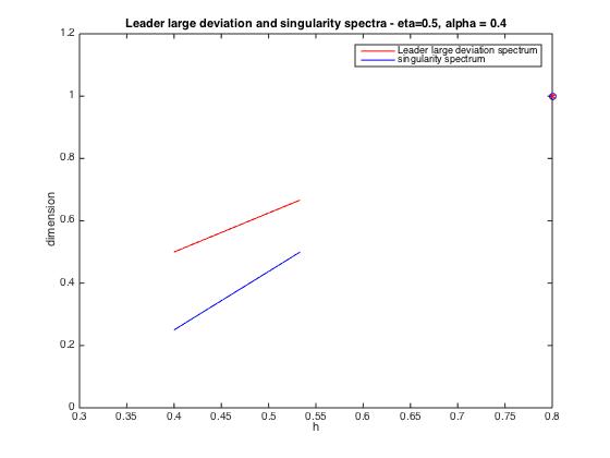
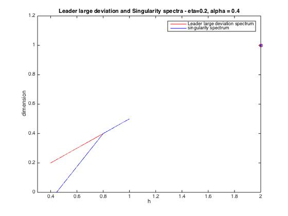
Figure 1: Large deviation and singularity spectra with $\alpha=0.4$ and $\eta=0.5$ (left), $\eta=0.2$ (right).

Before presenting the proof of this result in the following subsections, let us make a few comments and introduce some notations.

• In both cases, the Hausdorff dimension of the iso-Hölder set of the maximal finite regularity is exactly given by the Hausdorff dimension of the Cantor. This result is expected because it is clear that if $x$ is a point outside the Cantor $K$, then $\lambda_{j}(x)\notin\Gamma_{j}$ for $j$ large enough.

• One could of course replace in the model the coefficients $c_{\lambda}=0$ by $c_{\lambda}=2^{-\gamma j}$ with any exponent $\gamma$ larger than the maximal regularity on the Cantor set. It will give $\mathcal{D}_{f}(\gamma)=\rho_{f}(\gamma)=1$. It represented in Figure 3.

• For $j\geq 0$, we denote by $F_{j}$ the set

  $$F_{j}=\{\lambda\in\Lambda_{j}:\,c_{\lambda}=2^{-\alpha j}\}.$$

  Since one only needs to consider in $F_{j}$ dyadic intervals of $\Gamma_{j}$ and since $\#\Gamma_{j}=2^{3j/4}$, one directly gets

  $${\mathbb{E}}[\#F_{j}]=2^{\eta j}.$$

  The leader large deviation spectrum evaluted at $\alpha$ is equal to $\eta$, what could thus be expected.

• For every $j$, let us define the subset $R_{j}$ of $\Gamma_{j}$ by setting

  $$R_{j}=\{\lambda\in\Lambda_{j}:\lambda\cap K\neq\emptyset\}.$$

  The dyadic intervals of $\Gamma_{j}\setminus R_{j}$ will be removed in the following steps of the construction of the Cantor set $K$, up to step $2n$ since the set $C_{2n}$ contains dyadic intervals of length $2^{-j}$. In particular, one has $R_{j}=\{\lambda\in\Lambda_{j}:\lambda\cap C_{2n}\neq\emptyset\}$ and it follows that

  $$\#R_{j}=2^{j/2}.$$

  Even though their support will be removed in the construction of the Cantor set $K$, the coefficients associated to intervals of $R_{j}$ have nevertheless an influence on the wavelet leaders of points in $K$ and then on the spectra. This will clearly appear in the proof of Proposition 5.8.

• If one denotes by $G_{j}$ the subset of $F_{j}$ defined by

  $$G_{j}=\{\lambda\in R_{j}:c_{\lambda}=2^{-\alpha j}\},$$

  one obtains that

  $${\mathbb{E}}[\#G_{j}]=2^{(\eta-1/4)j}.$$

  We notice here that if $\eta<1/4$, there will be very few wavelet coefficients of order $2^{-\alpha j}$ at every scale $j$. More precisely, the supremum of the number of non-zero coefficients at scale $j$ whose support intersects $K$ will be almost surely bounded in $j$ as proved in Lemma 5.3 below. In particular, the regularity $\alpha$ might not be attained. This will be confirmed by Lemma 5.5 that shows that in this case, the minimal regularity is $\frac{2\alpha}{4\eta+1}$.

• Let us fix $\lambda\in R_{j}$. If $\lambda_{0}\subseteq\lambda$ is a dyadic interval of scale $j_{0}\leq 2j$, then $\lambda_{0}\in\Gamma_{j_{0}}$. A non-zero wavelet leader $d_{\lambda}=2^{-hj}$ for $h\leq 2\alpha$ comes from a non-zero coefficient $c_{\lambda_{0}}=2^{-\alpha j_{0}}\sim 2^{-hj}$ of scale $j_{0}$ of order $\frac{h}{\alpha}j\leq 2j$ and

  $$\#\{\lambda_{0}\subseteq\lambda:\lambda_{0}\in\Lambda_{j_{0}}\}=2^{j_{0}-j}.$$

  If we consider now the scale $j_{0}=2j+4$, only the dyadic subintervals of $\lambda$ of scale $j_{0}$ included in the first and the last quarter of $\lambda$ remain in $\Gamma_{j_{0}}$. Consequently,

  $$\#\{\lambda_{0}\subseteq\lambda:\lambda_{0}\in\Lambda_{j_{0}}\}=2^{j+3}<2^{j_{0}-j}.$$

  This explains the different behaviors in the computation of the multifractal sectrum, according to the position of $h$ with respect to $2\alpha$. Note that the second case corresponding to $h\geq 2\alpha$ will never occurs if the series is not too lacunar, that is if $\eta\geq 1/4$. Indeed in that case, the maximal regularity for the point of the Cantor set will be smaller than $2\alpha$, see Lemma 5.6.

The computation of the expectations of $F_{j}$ and $G_{j}$ together with Chebyshev inequality combined with Borel-Cantelli lemma give directly the following lemma.

Lemma 5.3

Almost surely, for every $\varepsilon>0$, there is $J\in\mathbb{N}$ such that

$$2^{(\eta-\varepsilon)j}\leq\#F_{j}\leq 2^{(\eta+\varepsilon)j}\quad\text{ and }\quad 2^{(\eta-1/4-\varepsilon)j}\leq\#G_{j}\leq 2^{(\eta-1/4+\varepsilon)j}$$

for every $j\geq J$.

Let us end this introduction to our model by providing the following concentration lemma. It states that the non-zero coefficients are well distributed and will be useful to obtain both large deviation and multifractal spectra.

Lemma 5.4

Almost surely, for every $\varepsilon>0$, there are infinitely many scales $j$ such that every interval of length $2^{-(\eta+1/4-\varepsilon)j}$ centered on dyadic numbers contains at most $2^{2\varepsilon j}$ non-zero coefficients of scale $j$.

Proof.  Let us fix $\varepsilon>0$. For every dyadic interval $\lambda\in\Lambda_{j}$, let us denote by $\lambda^{-b}$ the dyadic interval of scale $j-b$ that contains $\lambda$. Remark that the random variables that counts the number of non-zero coefficients of scale $j$ in a interval of length $2^{-(\eta+1/4-\varepsilon)j}$ centered on a dyadic interval of scale $j$ follows a binomial law Bin$(n,p)$ of parameters $n\leq 2^{(3/4-\eta+\varepsilon)j}$ and $p=2^{(\eta-3/4)j}$, so that its expectation is smaller than $2^{\varepsilon j}$. Let $A_{j}$ denote the event “there is a dyadic interval $\lambda\in\Lambda_{j}$ such that for all $b\in\{0,\dots,N-1\}$, the interval of length $2^{-(\eta+1/4-\varepsilon)(j-b)}$ centered on $\lambda^{-b}$ contains more than $2^{2\varepsilon(j-b)}$ non-zero coefficients”. Markov inequality leads to

$${\mathbb{P}}[A_{j}] \leq \sum_{\lambda\in\Lambda_{j}}\prod_{b=0}^{N-1}{\mathbb{P}}[\text{$\lambda^{-b}$ contains more than $2^{2\varepsilon(j-b)}$ non-zero coefficients}]$$

$$\leq \sum_{\lambda\in\Lambda_{j}}\prod_{b=0}^{N-1}2^{-\varepsilon(j-2b)}$$

$$\leq 2^{j(1-\varepsilon N)}2^{2\varepsilon(N-1)}$$

which is the general term of a convergent series if $N$ is large enough. $\Box$

5.1 Computation of $\mathcal{D}_{f}$

Let us start by studying the range for the possible values for the Hölder exponent of the points in the Cantor set. First, let us show that in the very lacunar case $\eta<1/4$, the regularity $\alpha$ is not observed. Consider $\beta<\frac{2\alpha}{4\eta+1}$. If there were a point $x_{0}\in K$ such that $h_{f}(x)=\beta$, we would have $d_{j}(x_{0})\geq 2^{-j(\beta+\varepsilon)}$ for infinitely many scales $j$ and some $\varepsilon\in(0,\frac{2\alpha}{4\eta+1}-\beta)$. But, because of the important lacunarity of the series, for $\eta<1/4$, the probability to have infinitely many intervals $\lambda$ which intersect the Cantor with a $c_{\lambda}\neq 0$ is null. Even more, as we will prove in the next lemma, with probablity equal to one, one needs to go at least $\frac{2\alpha}{4\eta+1}\log_{2}|\lambda|$ scales below before having a non-zero coefficient on a $\lambda^{\prime}\subset\lambda$.

Lemma 5.5

Let $\eta<1/4$. Almost surely, for all $x\in K$ one has $h_{f}(x)\geq\frac{2\alpha}{4\eta+1}$.

Proof.  Let us fix $h\in(\alpha,\frac{2\alpha}{4\eta+1})$ and let $A_{j}$ denote the event

$$A_{j}=\{\exists\lambda\in R_{j}\text{ such that }|d_{\lambda_{j}}|\geq 2^{-hj}\}.$$

Then

$${\mathbb{P}}[A_{j}] \leq \sum_{\lambda\in R_{j}}{\mathbb{P}}[\exists\lambda^{\prime}\subseteq 3\lambda\text{ such that }\lambda^{\prime}\in\Gamma_{l}\text{ with }j\leq\ell\leq\frac{h}{\alpha}j\text{ and }c_{\lambda^{\prime}}=2^{-\alpha\ell}]$$

$$\leq \sum_{\lambda\in R_{j}}\sum_{j\leq\ell\leq\frac{h}{\alpha}j}3\cdot 2^{\ell-j}2^{(\eta-3/4)\ell}$$

$$\leq 3\cdot 2^{-j/2}\sum_{j\leq\ell\leq\frac{h}{\alpha}j}2^{(\eta+1/4)\ell}$$

$$\leq 3\frac{h}{\alpha}j2^{-j/2}2^{(\eta+1/4)\frac{h}{\alpha}j}$$

which is the general term of a convergent series since $h<\frac{2\alpha}{4\eta+1}$. By taking a dense sequence $(h_{n})_{n\in\mathbb{N}}$ in $(\alpha,\frac{2\alpha}{4\eta+1})$, we get the conclusion. $\Box$

An upper bound of the maximal regularity - which will be proved to be optimal later - of the lacunary wavelet series is obtained in the following lemma and depends whereas $\eta\leq 1/4$ or not.

Lemma 5.6

Almost surely, there is $J\in\mathbb{N}$ such that

$$\sup_{\lambda^{\prime}\subseteq\lambda}|c_{\lambda^{\prime}}|\geq\begin{cases}2^{-\frac{\alpha}{2\eta}(j+\log_{2}j)}&\text{ if }0<\eta\leq 1/4,\\[6.45831pt] 2^{-\frac{\alpha}{\eta+1/4}(j+\log_{2}j)}&\text{ if }1/4<\eta<3/4.\end{cases}$$

for every $\lambda\in R_{j}$ with $j\geq J$. In particular, almost surely for all $x\in K$, one has $h_{f}(x)\leq\frac{\alpha}{\eta+1/4}$ if $0<\eta<1/4$ and $h_{f}(x)\leq\frac{\alpha}{2\eta}$ if $1/4\leq\eta<3/4$.

Proof.  We start with the easiest case $1/4<\eta<3/4$. Let $j\geq 0$ and let us define the event

$$A_{j}=\{\exists\lambda\in R_{j}\,\text{ such that }d_{\lambda}<2^{-\frac{\alpha}{\eta+1/4}(j-\log_{2}j)}\}.$$

Let us fix $j_{0}=\lfloor\frac{1}{\eta+1/4}(j+\log_{2}j)\rfloor$ so that $2^{-\alpha j_{0}}\geq 2^{-\frac{\alpha}{\eta+1/4}(j-\log_{2}j)}$. Using the assumption $\eta>1/4$, one gets $j_{0}\leq 2j$ for $j$ large enough. Consequently, if $\lambda\in R_{j}$, all the dyadic cubes $\lambda_{0}\subseteq\lambda$ of scale $j_{0}$ belong to $\Gamma_{j_{0}}$ and may then potentially have a non-zero coefficient. Consequently, the number of random dyadic intervals $\lambda_{0}\subseteq\lambda$ with $\lambda\in\Lambda_{j_{0}}$ is equal to $2^{j_{0}-j}$. As done in the proof of Lemma 4.2, the Borel-Cantelli lemma gives the conclusion.

In the case $\eta\leq 1/4$, we define similarly as previously

$$A_{j}=\{\exists\lambda\in R_{j}\,\text{ such that }d_{\lambda}<2^{-\frac{\alpha}{2\eta}(j+\log_{2}j)}\}.$$

Let $j_{0}=\lfloor\frac{1}{2\eta}(j+\log_{2}j)\rfloor$. Since $\eta\leq 1/4$, one has $j_{0}>2j$. Again, we need to count how many dyadic cubes $\lambda_{0}\subseteq\lambda$ belong to $\Gamma_{j_{0}}$. At the scale $m=2j$, all the possible dyadic cubes of size $2^{-m}$ are in $\Gamma_{m}$ because $\lambda$ intersects $K$ so is included in $C_{j/2}$. After that, the set losts half of its length each four steps and we find that, writing $\ell_{0}=j_{0}-2j$, it remains around $2^{j+3\ell_{0}/4}=2^{3j_{0}/4-j/2}$ dyadic cubes $\lambda_{j_{0}}\subseteq\lambda_{j}$ in $\Gamma_{j_{0}}$. Again, the Borel-Cantelli lemma allows to conclude. $\Box$

By combining Lemmas 5.5 and 5.6, we obtain that the Hölder exponent of any point of the Cantor set lies in $[\frac{2\alpha}{4\eta+1},\frac{\alpha}{2\eta}]$ if $\eta\leq 1/4$ and $[\alpha,\frac{\alpha}{\eta+1/4}]$ if $1/4<\eta<3/4$. Using the same arguments as in the proof of Corollary 4.3, we also get the following random covering of $K$.

Corollary 5.7

Almost surely, one has

$$K\subseteq\begin{cases}\displaystyle\limsup_{j\to+\infty}\bigcup_{k\in F_{j}}B\left(k2^{-j},2^{-2\eta(1-{\varepsilon_{j}})j}\right)&\text{ if }0<\eta\leq 1/4,\\[12.91663pt] \displaystyle\limsup_{j\to+\infty}\bigcup_{k\in F_{j}}B\left(k2^{-j},2^{-(\eta+\frac{1}{4})(1-{\varepsilon_{j}})j}\right)&\text{ if }1/4<\eta<3/4\end{cases}$$

where

$${\varepsilon_{j}}=\begin{cases}\frac{\log_{2}j}{2\eta j}&\text{ if }0<\eta\leq 1/4,\\[6.45831pt] \frac{\log_{2}j}{(\eta+1/4)j}&\text{ if }1/4<\eta<3/4.\end{cases}$$

Following the same idea as in the classical case, we consider for every $\delta\in(0,1]$ the random sets

$$E_{\delta}=\limsup_{j\rightarrow+\infty}\bigcup_{k\in F_{j}}B\left(k2^{-j},2^{-\delta(1-\varepsilon_{j})j}\right),$$

and

$$G_{\delta}:=K\cap\left(\bigcap_{0<\delta^{\prime}<\delta}E_{\delta^{\prime}}\setminus\bigcup_{\delta<\delta^{\prime}\leq 1}E_{\delta^{\prime}}\right)\ \text{ if }\ \delta<1\quad\text{ and }\quad G_{1}:=K\cap\bigcap_{0<\delta^{\prime}<1}E_{\delta^{\prime}}.$$

One has again that the iso-Hölder sets of the lacunary wavelet series are given by

$$G_{\delta}=\{x\in[0,1]:h_{f}(x)=\frac{\alpha}{\delta}\}$$

for every $\delta\in(0,1]$. It suffices then to compute the Hausdorff dimensions of the sets $G_{\delta}$ for $\delta$ in $[2\eta,\frac{4\eta+1}{2}]$ if $\eta\leq 1/4$ and in $[\eta+1/4,1]$ if $1/4<\eta<3/4$.

As in the classical case, the union and the intersection appearing in the definition of $G_{\delta}$ can be taken countable by considering subsequences converging to $\delta$. For this reason, in what follows, everything can be made countable by fixing a dense sequence $(\delta^{\prime}_{n})_{n\in\mathbb{N}}$ of $[0,1]$ and estimate the Hausdorff dimension of each $E_{\delta^{\prime}}$.

Proposition 5.8

1. If $\eta\in[1/4,3/4)$, then almost surely

   $$\dim_{\mathcal{H}}(G_{\delta})=\frac{\eta+1/4}{\delta}-\frac{1}{2}$$

   for every $\delta\in[\eta+1/4,1]$.

2. If $\eta\in(0,1/4]$, then almost surely

   $$\dim_{\mathcal{H}}(G_{\delta})=\begin{cases}\frac{\eta}{\delta}&\text{ if }\delta\in[2\eta,\frac{1}{2}]\\ \frac{\eta+1/4}{\delta}-\frac{1}{2}&\text{ if }\delta\in[\frac{1}{2},\frac{4\eta+1}{2}].\\ \end{cases}$$

Proof.  Let us start with the upper bound. Both cases are treated together. For every $\delta^{\prime}<\delta$ and $J\in\mathbb{N}$, we note that the set

$$\bigcup_{j\geq J}\bigcup_{k\in F_{j}}B\left(k2^{-j},2^{-\delta^{\prime}j}\right)\cap K$$

forms a covering of $G_{\delta}$. Since we intersect with $K$, for a fixed $j\geq J$, we have to count the number $N_{\delta^{\prime},j}$ of non-zero coefficients associated to dyadic intervals $\lambda_{j,k}$ wich are in $C_{\lfloor j/4\rfloor}$ and at a distance less than $2^{-\delta^{\prime}j}$ of the set $C_{\lfloor j/2\rfloor}$. It will then suffices to study the convergence of the series

$$\sum_{j\geq J}N_{\delta^{\prime},j}2^{-\delta^{\prime}sj}.$$

• If $\delta^{\prime}\leq 1/2$, then $2^{-\delta^{\prime}j}\geq 2^{-2n}$ for $j=4n$. Consequently, the considered intervals included in $C_{\lfloor j/4\rfloor}$ and at a distance less than $2^{-\delta^{\prime}j}$ of $C_{\lfloor j/2\rfloor}$ are all the intervals of $C_{\lfloor j/4\rfloor}$. Lemma 5.3 implies that $N_{\delta^{\prime}j}\leq 2^{(\eta+\varepsilon)j}$ so that

  $$\sum_{j\geq J}N_{\delta^{\prime},j}2^{-\delta^{\prime}sj}\leq\sum_{j\geq J}2^{(\eta+\varepsilon)j}2^{-\delta^{\prime}sj}<+\infty$$

  if $s>\frac{\eta+\varepsilon}{\delta^{\prime}}$, which implies in turn that $\dim_{\mathcal{H}}(G_{\delta})\leq\eta/\delta$.

  

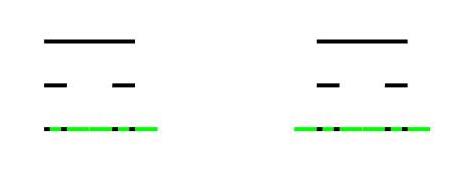
  Figure 2: The points at a distance less than $2^{-\delta^{\prime}j}$ of $C_{\lfloor j/2\rfloor}$ with $\delta^{\prime}\leq 1/2$ cover the set $C_{\lfloor j/4\rfloor}$.

• If $\delta^{\prime}>1/2$, we have to consider the $k\in F_{j}$ such that $\lambda_{j,k}$ is at a distance less than $2^{-\delta^{\prime}j}$ of the set $C_{\lfloor j/2\rfloor}$. Hence, we have to count the number of dyadic interval $\lambda_{j,k}$ wich are in $C_{\lfloor j/4\rfloor}$ and at a distance less than $2^{-\delta^{\prime}j}$ of $C_{l}$ where $l$ is of order $\delta^{\prime}j/2$ and is formed by intervals of length $2^{-\delta^{\prime}j}$. This number is bounded by $C2^{(1-\delta^{\prime}/2)j}$ for some constant $C$ independent of $j$. Using Markov inequality and the Borel Cantelli lemma as in Lemma 5.3, we get that almost surely, $N_{\delta^{\prime},j}\leq 2^{(1/4+\eta-\delta^{\prime}/2+\varepsilon)j}$. It follows that

  $$\sum_{j\geq J}N_{\delta^{\prime},j}2^{-\delta^{\prime}sj}\leq\sum_{j\geq J}2^{(1/4+\eta-\delta^{\prime}/2+\varepsilon)j}2^{-\delta^{\prime}sj}<+\infty$$

  if $s>\frac{1/4+\eta+\varepsilon}{\delta^{\prime}}-\frac{1}{2}$. It follows that $\dim_{\mathcal{H}}G_{\delta}\leq\frac{1/4+\eta}{\delta}-\frac{1}{2}$ on an event of probability one.

  

  

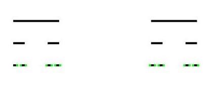
  Figure 3: The points at a distance less than $2^{-\delta^{\prime}j}$ of $C_{\lfloor j/2\rfloor}$ if $\delta^{\prime}>1/2$ give an intermediate step of the construction of the Cantor set.

Combining both cases together, we get the announced upper bounds. Let us now turn to the lower bounds. As done in the proof of Proposition 4.8, we simply need to estimate $\dim_{\mathcal{H}}(E_{\delta})$ from below. Then, classical properites of the Hausdorff dimension will give the conclusion.

Let us start by assuming that either $\eta>1/4$ and $\delta\geq\eta+1/4$, or $\eta\leq 1/4$ and $\delta>1/2$. In both cases, $\delta\geq 1/2$. Fix $\varepsilon>0$. As done previously, it suffices to consider in the definition of $E_{\delta}$ the non-zero coefficients $c_{j,k}$ where $\lambda_{j,k}$ belongs $C_{\lfloor j/4\rfloor}$ to and is at a distance at most $2^{-\delta j}$ of $C_{\lfloor j/2\rfloor}$, whose number is almost surely greater than $2^{(1/4+\eta-\delta/2-\varepsilon)j}$. From Lemma 5.4, we know that there are more than $2^{(1/4+\eta-\delta/2-2\varepsilon)j}$ non-zero coefficients located on distincts intervals of $C_{l}$, where $l$ is of order $\delta j/2$, since the size of an interval of $C_{l}$ is of order $2^{\delta j}\leq 2^{-(\eta+1/4-\varepsilon)j}$. The position of these coefficients can be seen as the position of the non-zero coefficients of a classical lacunary wavelet series $L$ on the Cantor $\bigcap_{l\in\mathbb{N}}C_{l}$ with $2^{(1/4+\eta-\delta/2-2\varepsilon)2l/\delta}$ non-zero coefficients located on intervals on length $2^{-2l}$. It corresponds to a lacunarity $\frac{1}{\delta}(1/4+\eta-\delta/2-2\varepsilon)$. The Hausdorff dimension of $E_{\delta}(f)$ is then larger than the Hausdorff dimension of the set $E_{1}(L)$ of minimal regularity of this new lacunary wavelet series. It follows from Proposition 4.8 that

$$\dim_{\mathcal{H}}E_{\delta}(f)\geq\frac{1/4+\eta-2\varepsilon}{\delta}-\frac{1}{2}.$$

Let us now focus on the case $\delta\in[2\eta,1/2]$ which only exists for $\eta\leq 1/4$. As in the classical case, we use an ubiquity argument. Note that the argument of the general mass transference could not have been applied in the case we just dealt for great values of $\delta$ for the following reason. The assumptions of Theorem 4.7 require that the balls are centered in $X=K$. For $\delta>1/2$, if $k2^{-j}\notin K$, the ball $B(k2^{-j},2^{-\delta j})$ of $E_{\delta}$ does not necessarily meet the Cantor set $K$ (even by multiplying the radius with a constant independent of $j$). At the opposite, if $\delta<1/2$, all balls $B(c_{j,k},2^{-\delta j})$ of $E_{\delta}$ intersects the Cantor $K$, and by doubling it we can suppose that each ball of $E_{\delta}$ is centered in $K$. Applying Theorem 4.7 as in the classical case thanks to Lemma 5.6, we get

$$\mathcal{H}^{\eta/\delta}\left(K\cap\limsup_{j\to+\infty}\bigcup_{k\in F_{j}}B(k2^{-j},2^{-\delta(1-{\varepsilon_{j}})j})\right)=\mathcal{H}^{\eta/\delta}(K)>0$$

since $\frac{\eta}{\delta}\leq\frac{1}{2}$. We conclude that $\dim_{\mathcal{H}}(E_{\delta})\geq\frac{\eta}{\delta}$. $\Box$

5.2 Computation of $\rho_{f}$

Let us explain the idea of the computation of the leader large deviation spectrum. Roughly speaking, a non-zero coefficient $c_{j,k}=2^{-\alpha j}$ will give birth to a wavelet leader equal to $2^{-hj^{\prime}}$ for $j^{\prime}=\tfrac{h}{\alpha}j$. Since the non-zero coefficients are well distributed on the Cantor set $K$ by Lemma 5.4, there will be at scale $j^{\prime}$ around $\#F_{j}$ wavelet leaders of order $2^{-hj^{\prime}}$. Lemma 5.3 implies then that $\rho_{f}(h)=\frac{h\eta}{\alpha}$. In particular, $\rho_{f}(\alpha)=\eta$ as expected.

Note that the possible values for $h$ are already known. Indeed, fom Lemma 5.6, we know that almost surely, the wavelet leaders associated to dyadic intervals $\lambda\in R_{j}$ satisfy

$$d_{\lambda}\geq\begin{cases}2^{-(\frac{\alpha}{2\eta}+\varepsilon)j}&\text{ if }0<\eta\leq 1/4\\ 2^{-(\frac{\alpha}{\eta+1/4}+\varepsilon)j}&\text{ if }1/4<\eta<3/4\end{cases}$$

for $j$ large enough. Dyadic intervals $\lambda\in\Gamma_{j}\setminus R_{j}$ contains less random dyadic subintervals appearing in the construction of $f$ than dyadic intervals of $R_{j}$, so that they cannot have smaller non-zero wavelet leaders.

More precisely, in the case $\eta\in(1/4,3/4)$, the same arguments as those of the proof of Lemma 5.6 give that almost surely, for the dyadic intervals $\lambda\in\Gamma_{j}\setminus R_{j}$ and for every $\varepsilon>0$, if $d_{\lambda}\neq 0$, then $d_{\lambda}\geq 2^{-(\frac{\alpha}{\eta+1/4}+\varepsilon)j}$ for $j$ large enough. Consequently the support of the large deviation spectra is included in $[\alpha,\frac{\alpha}{\eta+1/4}]$.

In the very lacunar case $\eta\in(0,1/4)$, we know that if $\lambda^{\prime}\subseteq\lambda$ is a dyadic interval of scale $j^{\prime}\geq 2j$ with $\lambda\in\Gamma_{j}\setminus R_{j}$, then $\lambda^{\prime}\notin\Gamma_{j^{\prime}}$. Consequently, the wavelet leader $d_{\lambda}$ is either equal to $0$ or to $2^{-\alpha j^{\prime}}$ with $j^{\prime}<2j$, in which case $d_{\lambda}\geq 2^{-2\alpha j}\geq 2^{-(\frac{\alpha}{2\eta})j}$. It follows that the support of the large deviation spectra is included in $[\alpha,\frac{\alpha}{2\eta}]$.

Proposition 5.9

Almost surely, one has

$$\rho_{f}(h)=\begin{cases}\frac{h\eta}{\alpha}&\text{ if }h\in[\alpha,h_{\max}]\\ 1&\text{ if }h=+\infty\\ -\infty&\text{otherwise.}\end{cases}$$

where

$$h_{\max}=\begin{cases}\frac{\alpha}{2\eta}&\text{ if }\eta\in(0,1/4]\\ \frac{\alpha}{\eta+1/4}&\text{ if }\eta\in(1/4,3/4).\end{cases}$$

Proof.  The result is clear if $h\notin[\alpha,h_{\max}]$. Let us then fix $h\in[\alpha,h_{\max}]$ and $\varepsilon>0$. For every scale $j$ large enough, one has almost surely

$$\#\{\lambda\in\Lambda_{j}:2^{-(h+\varepsilon)j}\leq d_{\lambda}\leq 2^{-(h-\varepsilon)j}\}\leq\sum_{j^{\prime}=\lfloor\frac{h-\varepsilon}{\alpha}j\rfloor}^{\lfloor\frac{h+\varepsilon}{\alpha}j\rfloor+1}\#F_{j^{\prime}}\leq Cj2^{(\eta+\varepsilon)\frac{h+\varepsilon}{\alpha}j}$$

for some constant $C>0$ and $j$ large enough, where we have used Lemma 5.3. The upper bound for $L_{f}(h)$ follows directly.

The lower bound in the case $\eta\in(0,1/4]$ and $h\in[2\alpha,\alpha/2\eta]$ follows directly from Propositions 2.9 and 5.8. Hence, we can assume that either $\eta\in(0,1/4]$ and $h<2\alpha$, or $\eta\in(1/4,3/4)$. Let $j^{\prime}$ be a scale such that every interval of length $2^{-(\eta+1/4-\varepsilon)j^{\prime}}$ contains at most $2^{2\varepsilon j^{\prime}}$ non-zero coefficients. We know from Lemma 5.4 that almost surely there are infinitely many such scales. Given $j=\lfloor\frac{\alpha}{h+\varepsilon}j^{\prime}\rfloor$, one direcly compute that $2^{-j}\leq 2^{-(\eta+1/4-\varepsilon)j^{\prime}}$. This relation implies that every $\lambda\in\Lambda_{j}$ contains at most $2^{2\varepsilon j^{\prime}}$ non-zero coefficients of scale $j^{\prime}$. Applying again Lemma 5.3, one gets

$$\#\{\lambda\in\Lambda_{j}:d_{\lambda}\geq 2^{-(h+\varepsilon)j}\}\geq\#F_{j^{\prime}}2^{-2\varepsilon j^{\prime}}\geq 2^{(\eta-3\varepsilon)\frac{h+\varepsilon}{\alpha}j}.$$

This inequality implies that almost surely

$$\nu_{f}(h):=\lim_{\varepsilon\to 0}\limsup_{j\to+\infty}\frac{\#\{\lambda\in\Lambda_{j}:d_{\lambda}\geq 2^{-(h+\varepsilon)j}\}}{\log(2^{j)}}\geq\frac{h\eta}{\alpha}$$

for every $h\in[\alpha,h_{\max}]$ if $\eta\in[1/4,3/4)$, and for every $h\in[\alpha,2\alpha)$ if $\eta\in(0,1/4]$. We now refer to Lemma 3.5 of [6] which states that $\nu_{f}$ is the increasing hull of $\rho_{f}$. This result leads to the conclusion since $\nu_{f}$ is strictly increasing. $\Box$

6 Functional spaces for which the formalism is generically non-valid (decreasing part)

In this section, we show that the validity of the formalisms based on the wavelet leaders is weak for the estimation of the decreasing part of the multifractal spectrum by exhibiting functional spaces on which these formalisms are generically not satisfied. The idea is similar to the one developped in Subsection 3.4.

A sequence $(\sigma_{j})_{j\in\mathbb{N}}$ of real positive numbers is called admissible if there is a constant $C>0$ such that

$$C^{-1}\sigma_{j}\leq\sigma_{j+1}\leq C\sigma_{j}$$

for every $j\in\mathbb{N}$. Under this assumption, if one sets

$$\underline{\sigma_{j}}=\inf_{k\in\mathbb{N}}\frac{\sigma_{j+k}}{\sigma_{k}}\quad\text{and}\quad\overline{\sigma_{j}}=\sup_{k\in\mathbb{N}}\frac{\sigma_{j+k}}{\sigma_{k}}$$

for every $j\in\mathbb{N}$, then the sequence $(\log\underline{\sigma_{j}})_{j\in\mathbb{N}}$ is subadditive and the sequence $(\log\overline{\sigma_{j}})_{j\in\mathbb{N}}$ is superadditive. Fekete’s lemma states that the limits

$$\underline{s}(\sigma)=\lim_{j\to\infty}\frac{\log\underline{\sigma_{j}}}{\log 2^{j}}\quad\text{and}\quad\overline{s}(\sigma)=\lim_{j\to\infty}\frac{\log\overline{\sigma_{j}}}{\log 2^{j}}$$

exists and are finite. They are defined as the lower and upper Boyd indices of $\sigma$ respectively. They can be seen as indicators to measure the dyadic growth of the admissible sequence. For example, if the sequence $\sigma$ behaves as a dyadic sequence up so some logarithmic correction, then $\underline{s}(\sigma)=\overline{s}(\sigma)$. On the other side, given any positive real numbers $\alpha<\beta$, one can construct an admissible sequence $\sigma$ such that

$$\underline{s}(\sigma)=\alpha\quad\text{and}\quad\overline{s}(\sigma)=\beta,$$

see e.g. [14, 31]. This sequence oscillates slowly (so that it is admissible) between the dyadic behaviors $2^{-\alpha j}$ and $2^{-\beta j}$. Indeed, for every $\varepsilon>0$, one can easily get the existence of a constant $D>0$ such that

(7) $$D^{-1}2^{j(\underline{s}(\sigma)-\varepsilon)}\leq\underline{\sigma_{j}}\leq\frac{\sigma_{j+k}}{\sigma_{k}}\leq\overline{\sigma_{j}}\leq D2^{j(\overline{s}(\sigma)+\varepsilon)}$$

for every $j,k\in\mathbb{N}$, and $\underline{s}(\sigma)$ and $\overline{s}(\sigma)$ are the smallest and the biggest quantities respectively satisfying this relation. Given an admissible sequence $\sigma$, Fekete introduced the so-called Besov spaces of generalized smoothness. He obtained that these spaces are well defined, in the sense that there are independant of the chosen wavelet basis. The link with Hölder spaces of generalized smoothness is done in [30]. In this paper, we will then adpot the definition based on the wavelet coefficients (equivalent at least if $\overline{s}(\sigma)-\underline{s}(\sigma)<2)$ .

Let $\sigma$ be an admissible sequence such that $\underline{s}(\sigma)>0$. We say that a function $f$ belongs to the Hölder space $\Lambda^{\sigma}([0,1])$ if the wavelet coefficients of $f$ satisfy

$$\|f\|_{\Lambda^{\sigma}([0,1])}:=\sup_{j\in\mathbb{N}}\sup_{k\in\{0,\dots,2^{j}-1\}}\sigma_{j}|c_{j,k}|<+\infty$$

The aim of this section is to prove that if $\underline{s}(\sigma)\neq\overline{s}(\sigma)$, a generic function of $\Lambda^{\sigma}([0,1])$ does not verify the multifractal formalism. It gives a complement of informations to the work done in [32], where the authors proved that an adapted formalism is generically satisfied in these spaces. Note however that none of the results imply the other.

Proposition 6.1

Let $\sigma$ be an admissible sequence such that $0<\underline{s}(\sigma)<\overline{s}(\sigma)$. The set of functions $f\in\Lambda^{\sigma}([0,1])$ which do not satisfy the formalism contains a dense open set. In particular, it is Baire generic.

Proof.  For every $N\in\mathbb{N}$, we set

$$\mathcal{C}_{N}=\left\{f\in\Lambda^{\sigma}([0,1]):\sigma_{j}2^{N}|c_{j,k}|\in\mathbb{N}\setminus\{0\}\,\,\forall j\in\mathbb{N}\,,\forall k\in\{0,\dots,2^{j}-1\}\right\}.$$

Let $U_{N}$ be the open set defined by

$$U_{N}=\left\{g\in\Lambda^{\sigma}([0,1]):\exists f\in\mathcal{C}_{N}\text{ such that }\|f-g\|_{\Lambda^{\sigma}([0,1])}<2^{-N-1}\right\}.$$

For any $g\in U_{N}$ with wavelet coefficients $(e_{j,k})$, there exists $f\in\mathcal{C}_{N}$ with wavelet coefficients $(c_{j,k})$ such that $\|f-g\|_{\Lambda^{\sigma}([0,1])}<2^{-N-1}$. It implies that

$$|e_{j,k}|\leq|c_{j,k}|+|e_{j,k}-c_{j,k}|\leq\sigma_{j}^{-1}(\|f\|_{\Lambda^{\sigma([0,1])}}+2^{-N-1})$$

and

$$|e_{j,k}|\geq|c_{j,k}|-|e_{j,k}-c_{j,k}|\geq 2^{-N}\sigma_{j}^{-1}-2^{-N-1}\sigma_{j}^{-1}=2^{-N-1}\sigma_{j}^{-1}.$$

It follows that if $g$ belongs to the set $\mathcal{R}$ defined by

$$\mathcal{R}=\bigcup_{N\in\mathbb{N}}U_{N},$$

then there is a constant $C>0$ such that its sequence of wavelet coefficients $(e_{j,k})$ satisfies

(8) $$C^{-1}\leq\sigma_{j}|e_{j,k}|\leq C$$

The assumption $\underline{s}(\sigma)\neq\overline{s}(\sigma)$ implies directly that

$$\underline{s}(\sigma)\leq\alpha:=\liminf_{j\to+\infty}\frac{\log\sigma_{j}}{\log 2^{j}}<\limsup_{j\to+\infty}\frac{\log\sigma_{j}}{\log 2^{j}}=:\beta\leq\overline{s}(\sigma).$$

In particular, using (7), the values of $\frac{\log e_{j,k}}{\log 2^{j}}$ oscillate uniformly in $k$ between the indices $\alpha$ and $\beta$. It follows than the Hölder exponent of $g$ is everywhere equal to $\alpha$.

However, since the sequence $(\sigma_{j})_{j\in\mathbb{N}}$ is admissible, it oscillates slowly. Hence, larger exponents are detected by the large deviation spectrum. Indeed, one knows that for every $\varepsilon>0$, there are infinitely many scales $j$ such that $\sigma_{j}\geq 2^{(\beta-\varepsilon)j}$. Let us fix such a scale $j$. Equation (7) gives

$$D^{-1}2^{(j^{\prime}-j)(\underline{s}(\sigma)-\varepsilon)}\leq\frac{\sigma_{j^{\prime}}}{\sigma_{j}}$$

for every $j^{\prime}\geq j$, so that

$$\sup_{j^{\prime}\geq j}\sigma_{j^{\prime}}^{-1}\leq D\sigma_{j}^{-1}\sup_{j^{\prime}\geq j}2^{(j-j^{\prime})(\underline{s}(\sigma)-\varepsilon)}\leq D\sigma_{j}^{-1}\leq D2^{-(\beta-\varepsilon)j}.$$

Equation (8) implies then that

$$\sup_{\lambda^{\prime}\subseteq 3\lambda(j,k)}|e_{\lambda^{\prime}}|\leq C\sup_{j^{\prime}\geq j}\sigma_{j^{\prime}}^{-1}\leq CD2^{-(\beta-\varepsilon)j}$$

for every $k\in\{0,\dots,2^{j}-1\}$.

To conclude, let us prove that the set $\bigcup_{N\in\mathbb{N}}\mathcal{C}_{N}$ is dense in $\Lambda^{\sigma}([0,1])$. If $g\in\Lambda^{\sigma}([0,1])$ and $\varepsilon>0$, we fix $N$ such that $2^{-N}<\varepsilon$ and we construct the function $f$ via its sequence of wavelet coefficients $c_{j,k}$ by setting

$$c_{j,k}=\begin{cases}\sigma_{j}^{-1}2^{-N}[\sigma_{j}2^{N}e_{j,k}]&\text{ if }\sigma_{j}2^{N}|e_{j,k}|\geq 2,\\ \sigma_{j}^{-1}2^{-N}&\text{ if }\sigma_{j}2^{N}|e_{j,k}|<2.\end{cases}$$

It follows that $c\in\mathcal{C}_{N}$ and $|\sigma_{j}2^{N}e_{j,k}-\sigma_{j}2^{N}c_{j,k}|\leq 1$, which implies

$$\sigma_{j}|e_{j,k}-c_{j,k}|=2^{-N}|\sigma_{j}2^{N}e_{j,k}-\sigma_{j}2^{N}c_{j,k}|\leq 2^{-N}<\varepsilon$$

for every $j,k$. $\Box$

References

- [1] P. Abry, S. Jaffard, and H. Wendt. A bridge between geometric measure theory and signal processing: Multifractal analysis. In G. Karlheinz, M. Lacey, J. Ortega-Cerdà, and M. Sodin, editors, Operator-Related Function Theory and Time-Frequency Analysis, to appear.
- [2] J.M. Aubry, F. Bastin, and S. Dispa. Prevalence of multifractal functions in spaces. J. Fourier Anal. Appl., 13(2):175?185, 2007.
- [3] J.M. Aubry, F. Bastin, S. Dispa, and S. Jaffard. The spaces : new spaces defined with wavelet coefficients and related to multifractal analysis. Int. J. Appl. Math. Stat., 7(Fe07):82–95, 2007.
- [4] J.M. Aubry and S. Jaffard. Random wavelet series. Comm. Math. Phys., 227:483–514, 2002.
- [5] E. Bacry, J. Delour, and J.F. Muzy. Multifractal random walk. Phys. Rev. E., 64:026103–026106, 2001.
- [6] F. Bastin, C. Esser, and S. Jaffard. Large deviation spectra based on wavelet leaders. Rev. Matem. Iberoamer., 32 (3):859–890, 2016.
- [7] F. Bastin, C. Esser, and L. Simons. Topology on new sequence spaces defined with wavelet leaders. J. Math. Anal. Appl., 431(1):317–341, 2015.
- [8] V. Beresnevich and S. Velani. A mass transference principle and the Duffin-Schaeffer conjecture for Hausdorff measures. Ann. of Math., 164:971–992, 2006.
- [9] C. Coiffard, C. Melot, and T. Willer. A family of functions with two different spectra of singularities. Journal of Fourier Analysis and Applications, 20:961–984, 2014.
- [10] I. Daubechies. Orthonormal bases of compactly supported wavelets. Comm. Pure App. Math., 41:909–996, 1988.
- [11] I. Daubechies. Ten Lectures on Wavelets. CBMS-NSF Regional Conference Series in Applied Mathematics, 1992.
- [12] C. Esser, T. Kleyntssens, and S. Nicolay. A multifractal formalim for non-concave and non-increasing spectra: The leaders profile method. Appl. Comput. Harmon. Anal., 43 (2):269–291, 2017.
- [13] K. Falconer. The Geometry of Fractal Sets. Cambridge University Press, 1986.
- [14] W. Farkas and H.G. Leopold. Characterisations of function spaces of generalised smoothness. Ann. Mat. Pura Appl. (4), 185(1):1–62, 2006.
- [15] A. Fraysse. Generic validity of the multifractal formalism. SIMA - SIAM J. Math. Anal., 39 (2):593–607, 2007.
- [16] A. Fraysse and S. Jaffard. How smooth is almost every function in a Sobolev space ? Rev. Matem. Iberoamer., 22,N.2:663–682, 2006.
- [17] S. Jaffard. Pointwise smoothness, two-microlocalization and wavelet coefficients. volume 35, pages 155–168. 1991. Conference on Mathematical Analysis (El Escorial, 1989).
- [18] S. Jaffard. Construction de fonctions multifractales ayant un spectre de singularités prescrit. C.R.A.S., Vol. 315 Série 1, 1992.
- [19] S. Jaffard. The spectrum of singularities of Riemann’s function. Rev. Mat. Iberoamericana, 12(2):441–460, 1996.
- [20] S. Jaffard. Multifractal formalism for functions part I: Results valid for all functions. SIAM J. Math. Anal., 28:944–970, 1997.
- [21] S. Jaffard. Multifractal formalism for functions part II: Self-similar functions. SIAM J. Math. Anal., 28:971–998, 1997.
- [22] S. Jaffard. Lacunary wavelet series. Annals of Applied Probability., Vol. 10, No. 1, 2000.
- [23] S. Jaffard. On the Frisch–Parisi conjecture. J. Math. Pures Appl., 79:525–552, 2000.
- [24] S. Jaffard. Beyond Besov spaces part 1: Distributions of wavelet coefficients. J. Fourier Anal. Appl., 10:221–246, 2004.
- [25] S. Jaffard. Wavelet techniques in multifractal analysis, fractal geometry and applications: A jubilee of Benoit Mandelbrot. Proceedings of Symposia in Pure Mathematics, 72:91–151, 2004.
- [26] S. Jaffard. Beyond Besov spaces part 2: Oscillation spaces. Constr. Approx., 21:29–61, 2005.
- [27] S. Jaffard, P. Abry, S. G. Roux, B. Vedel, and H. Wendt. The contribution of wavelets in multifractal analysis. In Wavelet methods in Mathematical Analysis and Engineering. Higher Education Press, in Series in Contemporay Applied Mathematics, 2010.
- [28] S. Jaffard, B. Lashermes, and P. Abry. Wavelet leaders in multifractal analysis. In Wavelet analysis and applications, Appl. Numer. Harmon. Anal., pages 201–246. Birkhäuser, Basel, 2007.
- [29] T. Kleyntssens, C. Esser, and S. Nicolay. An algorithm for computing non-concave multifractal spectra using the spaces. Commun. Nonlinear Sci. Numer. Simul., 56:526–543, 2018.
- [30] D. Kreit and S. Nicolay. Characterizations of the elements of generalized Hölder-Zygmund spaces by means of their representation. J. Approx. Theory, 172:23–36, 2013.
- [31] T. Kühn, H.G. Leopold, W. Sickel, and L. Skrzypczak. Entropy numbers of embeddings of weighted Besov spaces. II. Proc. Edinb. Math. Soc. (2), 49(2):331–359, 2006.
- [32] L. Loosveldt and S. Nicolay. Generalized spaces of pointwise regularity: toward a general framework for the WLM. Nonlinearity, 34(9):6561–6586, 2021.
- [33] S. Mallat. A Wavelet Tour of Signal Processing. Academic Press, 1999.
- [34] P. Mattila. Geometry of sets and measures in Euclidean spaces: Fractals and rectifiability. Cambridge University Press, 1995.
- [35] Y. Meyer and D. Salinger. Wavelets and Operators, volume 1. Cambridge university press, 1995.
- [36] J.F. Muzy, E. Bacry, and A. Arneodo. Multifractal formalism for fractal signals: The structure function approach versus the wavelet-transform mudulus-maxima method. Phys. Rev. E, 47:875–884, 1993.
- [37] G. Parisi and U. Frisch. On the singularity structure of fully developed turbulence. Turbulence and Predictability in Geophysical Fluid Dynamics, pages 84–87, 1985.
- [38] S. Seuret. Multifractal analysis and wavelets. In Lecture notes from the CIMPA school, New trends in harmonic analysis, 2013.
- [39] H. Triebel. Theory of function spaces III. Monographs in Mathematics. Birkhäuser, 2006.
- [40] K. Weierstraß. Über continuirliche Functionen eines reellen Arguments, die für keinen Werth des letzteren einen bestimmten Differentialquotienten besitzen. Springer, 1988.