Nonparametric Embeddings of Sparse High-Order Interaction Events

Abstract

High-order interaction events are common in real-world applications. Learning embeddings that encode the complex relationships of the participants from these events is of great importance in knowledge mining and predictive tasks. Despite the success of existing approaches, e.g., Poisson tensor factorization, they ignore the sparse structure underlying the data, namely the occurred interactions are far less than the possible interactions among all the participants. In this paper, we propose Nonparametric Embeddings of Sparse High-order interaction events (NESH). We hybridize a sparse hypergraph (tensor) process and a matrix Gaussian process to capture both the asymptotic structural sparsity within the interactions and nonlinear temporal relationships between the participants. We prove strong asymptotic bounds (including both a lower and an upper bound) of the sparsity ratio, which reveals the asymptotic properties of the sampled structure. We use batch-normalization, stick-breaking construction and sparse variational GP approximations to develop an efficient, scalable model inference algorithm. We demonstrate the advantage of our approach in several real-world applications.

1 Introduction

Many real-world applications are filled with interaction events between multiple entities or objects, e.g., the purchases happened among customers, products and shopping pages at Amazon.com, and tweeting between twitter users and messages. Embedding these events, namely, learning a representation of the participant objects to encode their complex relationships, is of great importance and interest, in discovering hidden patterns from data, e.g., clusters and outliers, and performing downstream tasks, such as recommendation and online advertising.

While Poisson tensor factorization is a popular framework for the representation learning of those events, current methods, e.g., (Chi and Kolda,, 2012; Hansen et al.,, 2015; Hu et al., 2015b, ; Schein et al.,, 2015, 2016, 2019), are mostly based on a multilinear factorization form, e.g., (Tucker,, 1966; Harshman,, 1970), and therefore might be inadequate to estimate complex, nonlinear temporal relationships in data. More important, existing methods overlook the structural sparsity underlying these events. That is, the observed interactions are far less than all the possible interactions among the participants (e.g., 0.01%). Many factorization models rely on tensor algebras and demand all the tensor entries (i.e., interactions) should be observed (Kolda and Bader,, 2009; Kang et al.,, 2012; Choi and Vishwanathan,, 2014). Even for those entry-wise factorization models  (Rai et al.,, 2014; Zhao et al.,, 2015; Du et al.,, 2018), from the Bayesian viewpoint, they are equivalent to first generating the entire tensor and then marginalizing out the unobserved entries. In practice, however, the observed interactions are often very sparse, and their proportion can get even smaller with the increase of objects. For example, in online shopping, with the growth of users and items, the number of actual purchases (while growing) takes a smaller percentage of all possible purchases, i.e., all (user, item, shopping-page) combinations, because the latter grows much faster.

In this paper, we propose NESH, a novel nonparametric Poisson factorization approach for high-order interaction events embedding. Not only does NESH flexibly estimate various nonlinear temporal relationships of the participants, it also can capture structural sparsity within the present interactions, absorbing both the structural traits and hidden relationships into the embeddings. Our major contributions are the following:

• Model. We hybridize the recent sparse tensor (hypergraph) processes (STP) (Tillinghast and Zhe,, 2021) and matrix Gaussian processes (MGP) to develop a sparse event model, where the embeddings are in charge of both generating the interactions and modulating the event rates, hence can jointly encode the temporal relationships and sparse structure knowledge.

• Theory. We use Poisson tail estimate, Bernstein’s inequality and L’Hôpital’s rule to prove strong asymptotic bounds of the sparsity ratio, including both a lower and upper bound. The prior work Tillinghast and Zhe, (2021) only shows the sparsity ratio of the sampled tensors asymptotically converges to zero, yet never gives an estimate of the convergence rate. Our new result reveals more theoretical insight of STP in producing sparse structures, and can also characterize the classical sparse graph generation models (Caron and Fox,, 2014; Williamson,, 2016).

• Algorithm. We use the stick-breaking construction of the normalized hypergraph process to compute the embedding prior, and then use batch-normalization and variational sparse GP framework to develop an efficient and scalable model estimation algorithm.

For evaluation, we conducted simulations to demonstrate that our theoretical bounds can indeed match the actual sparsity ratio and capture the asymptotic trend. Hence they can provide a reasonable convergence rate estimate and characterize the behavior of the prior. We then tested our approach NESH on three real-world datasets. NESH achieves much better predictive performance than the existing methods that use Poisson tensor factorization, additional time steps, local time dependency windows and triggering kernels. NESH also outperforms the same model with the sparse hypergraph prior removed, which demonstrates the importance of accounting for the structure sparsity. We then looked into the embeddings estimated by NESH, and found interesting patterns, including the clusters of users, sellers, and item categories in online shopping, and groups of states where car crash accidents happened.

2 Background

We assume that we observed $K$-way interactions among $K$ types of objects or entities (e.g., customers, products and sellers). We denote by $D_{k}$ the number of objects of type $k$, and index each object by $i_{k}$ ($1\leq i_{k}\leq D_{k}$). We then index a particular interaction by a tuple ${\bf i}=(i_{1},\ldots,i_{K})$. We may observe multiple occurrences of a particular interaction. We denote the sequence of these events by ${\bf s}_{{\bf i}}=[s_{{\bf i}1},\ldots,s_{{\bf i}m_{{\bf i}}}]$ where $s_{{\bf i}j}$ is the time-stamp when $j$-th event occurred ($1\leq j\leq m_{\bf i}$) and $m_{{\bf i}}$ is the total number of the occurrences of ${\bf i}$. Suppose we have observed events of a collection of interactions, ${\mathcal{S}}=\{{\bf s}_{{\bf i}_{1}},\ldots,{\bf s}_{{\bf i}_{N}}\}$, we aim to learn an embedding for each participant object. Note that one object may participate in multiple, distinct interactions. We denote by ${\bf u}^{k}_{j}$ the embeddings for object $j$ of type $k$, which is an $R$ dimensional vector. We stack the embeddings of the objects of type $k$ into a embedding matrix ${\bf U}^{k}=[{\bf u}^{k}_{1},\ldots,{\bf u}^{k}_{D_{k}}]^{\top}$, and denote by ${\mathcal{U}}=\{{\bf U}^{1},\ldots,{\bf U}^{K}\}$ all the embedding matrices.

To estimate the embeddings from ${\mathcal{S}}$, a popular approach is tensor factorization. We can introduce a $K$-mode tensor ${\mathcal{Y}}\in\mathbb{R}^{D_{1}\times\ldots\times D_{K}}$ accordingly, where each mode $k$ includes $D_{k}$ objects, and each entry ${\bf i}$ corresponds to an event sequence ${\bf s}_{{\bf i}}$. For event modeling, we can use the popular (homogeneous) Poisson processes, and the probability of ${\bf s}_{{\bf i}}$ is given by

$$p(s_{{\bf i}}|\lambda_{{\bf i}})=e^{-\int_{0}^{T}\lambda_{{\bf i}}{\rm d}t}\prod\nolimits_{j=1}^{m_{{\bf i}}}\lambda_{{\bf i}}=e^{-T\lambda_{{\bf i}}}\lambda_{{\bf i}}^{m_{\bf i}},$$ (1)

where $T$ is the total time span of all the event sequences, and $\lambda_{{\bf i}}>0$ is the rate (or intensity) of the interaction ${\bf i}$. Since the probability is only determined by the event count, we can place the count value $m_{\bf i}$ in the entry ${\bf i}$ of ${\mathcal{Y}}$, and perform count tensor factorization. Classical tensor factorization approaches include Tucker decomposition (Tucker,, 1966), CANDECOMP/PARAFAC (CP) decomposition (Harshman,, 1970), etc. Tucker decomposition assumes ${\mathcal{Y}}={\mathcal{W}}\times_{1}{\bf U}^{1}\times_{2}\ldots\times_{K}{\bf U}^{K}$, where $\mathcal{W}\in\mathbb{R}^{r_{1}\times\ldots\times r_{K}}$ is a parametric core tensor, $\{{\bf U}^{k}|1\leq k\leq K\}$ are embedding matrices, and $\times_{k}$ is the tensor-matrix product at mode $k$ (Kolda,, 2006), which is very similar to the matrix-matrix product. If we set all $r_{k}=R$, and constrain ${\mathcal{W}}$ to be diagonal, Tucker decomposition is reduced to CANDECOMP/PARAFAC (CP) decomposition (Harshman,, 1970). While numerous tensor factorization algorithms have been developed, e.g., (Chu and Ghahramani,, 2009; Kang et al.,, 2012; Choi and Vishwanathan,, 2014), most of them inherit the CP or Tucker form. To perform count tensor factorization, we can use Poisson process likelihood (1) for each entry, and apply the Tucker/CP decomposition to the rates $\{\lambda_{{\bf i}}\}$ or log rates $\{\log(\lambda_{{\bf i}})\}$  (Chi and Kolda,, 2012; Hu et al., 2015b, ). A more refined strategy is to further partition the events into a series of time steps, e.g., by weeks or months, augment the count tensor with a time-step mode (Xiong et al.,, 2010; Schein et al.,, 2015, 2016, 2019), and jointly estimate the embeddings of these steps, $\{{\bf s}_{1},{\bf s}_{2},\ldots\}$. We can also model the dependencies between the time steps with some dynamics, e.g., (Xiong et al.,, 2010).

3 Model

Despite the success of existing Poisson tensor factorization approaches, they might be restricted in that (1) the commonly used CP/Tucker factorization over the rates are multilinear to the embeddings and therefore cannot capture more complex, nonlinear relationships between the interaction participants; (2) the homogeneous assumption, i.e., constant event rate, might be oversimplified, overlook temporal variations of the rates, and hence miss critical temporal patterns. More important, (3) in many real-world applications, the present interactions are very sparse, when contrasted to all possible interactions. For example, despite the massive online transactions, the ratio between the number of actual transactions and all possible transactions (i.e., all combinations of (customer, product, seller) is tiny, slightly above zero (e.g., $0.01\%$). This proportion can get even smaller with the growth of customers, products and sellers, because their combinations can grow much faster. Similar observations can be found in clicks in online advertising, message tweeting, etc. Existing methods, however, are not aware of this data sparsity, and lack an effective modeling framework to embed the underlying sparse structures. To overcome these limitations, we propose NESH, a novel nonparametric embedding model for sparse high-order interaction events, presented as follows.

3.1 Nonparametric Sparse Event Modeling for High-Order Interactions

First, to highlight the sparse structure within the observed events, we view the participants as nodes, and their interactions as $K$-way hyperedges in a hypergraph. Each edge connects $K$ participants (nodes), corresponding to a particular interaction ${\bf i}$. Attached to ${\bf i}$ is a sequence of events ${\bf s}_{\bf i}$ — the occurrence history of ${\bf i}$. Our goal is to learn an embedding for each node, which is able to not only estimate the complex temporal relationships between the nodes, but also capture the traits of the sparse hypergraph structure. To this end, we follow (Tillinghast and Zhe,, 2021; Caron and Fox,, 2014) to construct a stochastic process to sample the hypergraph, with a guarantee of sparsity in the asymptotic sense. Specifically, for each node type $k(1\leq k\leq K)$, we sample a set of Gamma processes (Hougaard,, 1986; Brix,, 1999) to represent an infinite number of nodes and their weights,

$$W^{\alpha}_{k,r}\sim\Gamma\text{P}(\beta_{\alpha})\;\;(1\leq k\leq K,1\leq r\leq R)$$ (2)

where $\beta_{\alpha}$ is a Lebesgue base measure confined to $[0,\alpha](\alpha>0)$. Next, we use these $\Gamma$Ps to construct a product-measure sum, with which as the mean measure to sample a Poisson point process (PPP) (Kingman,, 1992), which represents the sampled edges of the hypergraph,

$$M=\sum\nolimits_{r=1}^{R}W^{\alpha}_{1,r}\times\ldots\times W^{\alpha}_{K,r},\,\,$$

$$T|\{W^{\alpha}_{k,r}\}_{1\leq k\leq K,1\leq r\leq R}\sim\text{PPP}(M).$$ (3)

Accordingly, $T$ has the following form,

$$T=\sum_{{\bf i}\in{\mathcal{E}}}c_{{\bf i}}\cdot\delta_{\Theta^{\alpha}_{\bf i}},$$

where each point represents an hyperedge (interaction), ${\mathcal{E}}$ is the set of all the sampled points, $c_{{\bf i}}>0$ is the count of the point ${\bf i}$, and $\Theta^{\alpha}_{{\bf i}}=\{(\theta^{\alpha}_{1i_{1}},\ldots,\theta^{\alpha}_{Ki_{K}})\}$ represents the location of that point and comes from the $\Gamma$Ps, and $\delta_{[\cdot]}$ is the Dirac measure. In essence, the $\Gamma$Ps sample infinite nodes for each type $k(1\leq k\leq K)$, and then the PPP picks the nodes from each type to sample the hyperedges, i.e., multiway interactions.

To examine the sparsity, we look into the nodes in the sampled hyperedges ${\mathcal{E}}$, which are referred to as “active” nodes. They are participants of the interactions. For example, if an edge $2-3-1$ is sampled, then node 2, 3, 1 (of type 1, 2, 3 respectively) are active nodes. Denote by $D_{k}^{\alpha}$ the number of distinct active nodes of type $k$. If we connect all the active nodes of the $K$ types, we will have $\prod_{k=1}^{K}D_{k}^{\alpha}$ hyperedges (interactions) in total, i.e., the volume. Sparsity means the proportion of the sampled edges in all possible edges is very small, and the former grows slower than the latter, with the increase of active nodes. Denote by $N^{\alpha}$ the number of sampled edges. The sparsity is guaranteed by

Lemma 3.1 (Corollary 3.1.1 (Tillinghast and Zhe,, 2021)).

$N^{\alpha}=o(\prod_{k=1}^{K}D^{\alpha}_{k})$ almost surely as $\alpha\rightarrow\infty$, i.e., $\underset{\alpha\rightarrow\infty}{\lim}\frac{N^{\alpha}}{\prod_{k=1}^{K}D^{\alpha}_{k}}=0\;\;\;a.s.$

Note that this is an asymptotic notion of structural sparsity — with the hyper-graph volume growing (i.e., increasing $\alpha$), the proportion of the sampled edges is tending to zero. It is different from other notions (Choi and Vishwanathan,, 2014; Hu et al., 2015a, ) where the sparsity means data is dominated by zero values.

Given the sparse hypergraph prior, we then sample the observed edges (interactions) and associated events, $\mathcal{D}=\{({\bf i}_{1},{\bf s}_{{\bf i}_{1}}),\ldots,({\bf i}_{N},{\bf s}_{{\bf i}_{N}})\}$. Since they are always finite, we can use the standard PPP construction (Kingman,, 1992) to sample these observations, which is computationally much more convenient and efficient. Specifically, we normalize the mean measure $M=\sum_{r=1}^{R}W^{\alpha}_{1,r}\times\ldots\times W^{\alpha}_{K,r}$ in (3) to obtain a probability measure, and use it to sample the $N$ points (i.e., edges/interactions) independently. To normalize $M$, we need to first normalize each $\Gamma$P $W^{\alpha}_{k,r}(1\leq k\leq K,1\leq r\leq R)$, which gives a Dirichlet process (DP) (Ferguson,, 1973), with the strength as $\beta_{\alpha}([0,\alpha])=\alpha$, and base measure as the normalized base measure of $W^{\alpha}_{k,r}$ that is a uniform distribution in $[0,\alpha]$,

$$G^{k}_{r} \sim\text{DP}\big{(}\alpha,\text{Uniform}([0,\alpha])\big{)},$$ (4)

where $1\leq k\leq K$ and $1\leq r\leq R$. The normalized $M$ is $\frac{1}{R}\sum_{r=1}^{R}G^{1}_{r}\times\ldots\times G^{K}_{r}$. To capture rich structural information, we follow “Model-II” in (Tillinghast and Zhe,, 2021) to sample multiple DP weights for each node. Specifically, we drop the locations, and only sample the weights, which follow the GEM distribution (Griffiths,, 1980; Engen,, 1975; McCloskey,, 1965), and obtain

$$\widehat{G}_{r}^{k}=\sum_{j=1}^{\infty}\omega^{k}_{rj}\cdot\delta_{j}.$$ (5)

Accordingly, we construct a probability measure over all possible edges (interactions),

$${\widehat{M}}=\sum_{{\bf i}=(1,\ldots,1)}^{(\infty,\ldots,\infty)}w_{{\bf i}}\cdot\delta_{{\bf i}},$$ (6)

where $w_{{\bf i}}=\frac{1}{R}\sum_{r=1}^{R}\prod_{k=1}^{K}\omega_{ri_{k}}^{k}$. We then sample each observed interaction ${\bf i}_{n}\sim{\widehat{M}}$, and the probability is

$$p({\mathcal{E}})=\prod\nolimits_{n=1}^{N}p({\bf i}_{n})=\prod\nolimits_{n=1}^{N}w_{{\bf i}_{n}}.$$ (7)

Now, it can be seen that from (4) and (5), for each node $j$ of type $k$, we have sampled a set of $R$ weights $\{\omega^{k}_{1j},\ldots,\omega^{k}_{Rj}\}$ from $R$ DPs. From (6), we can see these weights reflect the activity of the node interacting with other nodes (of different types). Each weight naturally represents the sociability in one community/group, and these communities are overlapping. We use these sociabilities to construct the embeddings of the nodes. Therefore, they encode the sparse structural information underlying the observed interactions

Given the sampled interactions ${\mathcal{E}}$, we then sample their occurred events ${\mathcal{S}}=[{\bf s}_{{\bf i}_{1}},\ldots,{\bf s}_{{\bf i}_{N}}]$. To flexibly capture the temporal patterns, we use non-homogeneous Poisson processes. For each observed interaction ${\bf i}_{n}$, we consider a raw rate function $\rho_{{\bf i}_{n}}(t)$, and then link it to a positive rate function by taking the square, $\lambda_{{\bf i}_{n}}(t)=\left(\rho_{{\bf i}_{n}}(t)\right)^{2}$. Note that we can also use $\exp(\cdot)$, which, however, performs worse in our experiments. In order to capture the complex relationships of the rate functions and their temporal variations, we jointly sample the collection of rate functions, $\bm{\rho}=\{\rho_{{\bf i}_{n}}(t)|1\leq n\leq N\}$, from a matrix Gaussian process (MPG) (Rasmussen and Williams,, 2006),

$$\bm{\rho}\sim{\mathcal{M}\mathcal{N}}({\bf 0};\kappa_{1}({\bf x}_{{\bf i}},{\bf x}_{{\bf i}^{\prime}}),\kappa_{2}(t,t^{\prime})),$$ (8)

where $\kappa_{1}(\cdot,\cdot)$ is the (row) covariance function across different interactions (hyperedges), the inputs are the embeddings of participant nodes, ${\bf x}_{\bf i}=[{\bf u}^{1}_{i_{1}};\ldots;{\bf u}^{K}_{i_{K}}]$, and $\kappa_{2}(\cdot,\cdot)$ is the (column) covariance function about the time. We can choose nonlinear kernels for $\kappa_{1}$ and $\kappa_{2}$ to capture the complex relationships and temporal dependencies within $\bm{\rho}$. Given the rate functions, we then sample the observed event sequences from

$$p({\mathcal{S}}|\bm{\lambda})=$$

$$\prod_{n=1}^{N}\exp(-\int_{0}^{T}\left(\rho_{{\bf i}_{n}}(t)\right)^{2}{\rm d}t)\prod_{j=1}^{m_{{\bf i}_{n}}}\left(\rho_{{\bf i}}(s_{{\bf i}_{n}j})\right)^{2},$$ (9)

where $T$ is the total time span across all the event sequences.

From (7) and (9), we can see that, via coupling the DPs and matrix GP, both the structural properties in the sparsely observed interactions and hidden temporal relationships of the participant nodes in the events can be grasped and absorbed into the embeddings.

3.2 Theoretical Analysis of Sparsity

Although Tillinghast and Zhe, (2021) has proved the asymptotic sparsity guarantee of the hypergraph process in (3) (referred to as sparse tensor process in their paper), i.e., Lemma 3.1, the conclusion is rough in that we have no idea how the sparsity of the sampled hyper-graph varies along with more and more active nodes. We only know that at the limit, the sparsity ratio becomes zero. While Caron and Fox, (2014) gave some convergence rate estimate in their binary graph generating models under a similar modeling framework, the estimate is only available when using generalized $\Gamma$Ps (G$\Gamma$Ps) (Hougaard,, 1986) with a particular parameter range (see Theorem 10 in their paper). The estimate is not available for the popular ordinary $\Gamma$Ps as in our model. G$\Gamma$Ps cannot be normalized as DPs and are much harder/inconvenient for computation and inference. To extract more theoretical insight, we prove asymptotic bounds of the sparsity ratio for our hyper-graph process, which not only deepen our understanding of the properties of the sampled structures, but also fill the gap of prior works.

Lemma 3.2.

For a sparse hyper-graph process defined as in (3), for all sufficiently large $\alpha$, there exists an absolute constant $C>0$ such that, with probability at least $1-(C\alpha)^{-K}$,

$$\frac{e^{-1.03(2K)^{1/K}K(\log\alpha)^{1/K}}}{2K\log\alpha}\cdot\left[\frac{1.82}{(K-1)\log(1.01\alpha)}\right]^{K}$$

$$\leq\frac{N^{\alpha}}{\prod_{k=1}^{K}D_{k}^{\alpha}}\leq\left[\frac{2.11}{(K-1)\log(0.99\alpha)}\right]^{K}.$$

Proof sketch. We first use concentration inequalities, including Poisson tail estimate (Vershynin,, 2018) and Bernstein’s inequality, and L’Hopital’s rule to bound the measure of each $\Gamma$P on $[0,\alpha]$, and then take a union bound over $k=1\ldots K$ to obtain an upper bound of $N^{\alpha}$. The lower bound is more technical, and requires a careful estimate of the support of the intensity measure that appears in the sampled entries with high probability, for which we apply a novel probabilistic argument. We mainly combine Poisson tail estimates, union bounds, the Bernoulli distribution and L’Hôpital’s rule to bound each $D_{k}^{\alpha}$ and then derive the lower bound of $N^{\alpha}$. We leave the details in Appendix.

4 Algorithm

The matrix GP in our model, coupled with DPs, is computational costly. When the number of present interactions and/or the number of their events are large, we will have to compute a huge row and/or column covariance matrix, their inverse and determinants, which is very expensive or even infeasible. To address these issues, we use the stick-breaking construction (Sethuraman,, 1994), sparse variational GP approximation (Titsias,, 2009; Hensman et al.,, 2013) and batch normalization (Ioffe and Szegedy,, 2015) to develop an efficient, scalable variational inference algorithm.

Specifically, we use the stick-breaking construction to sample the DP weights (or GEM distribution),

$$v^{k}_{rj}\sim\text{Beta}(1,\alpha),\;\;\omega^{k}_{rj}=v^{k}_{rj}\prod\nolimits_{l=1}^{j-1}(1-v^{k}_{rl}),\;\;\;$$ (10)

where $1\leq j\leq\infty$. Therefore, we only need to estimate the stick-breaking variables $\{v^{k}_{rj}\}$, from which we can outright calculate the weights (or sociabilities). Since these weights can be very small and close to zero, we use their logarithm to construct the embedding of each node $j$ of type $k$, ${\bf u}^{k}_{j}=[\log(\omega^{k}_{1j});\ldots;\log(\omega^{k}_{Rj})]$.

Next, to conveniently handle the matrix GP prior in (8), we unify all the raw rate functions as one function of the embeddings and time, $\rho_{{\bf i}}(t)=f({\bf x}_{{\bf i}},t)$, over which we assign a GP prior with a product covariance (kernel) function, $\kappa([{\bf x}_{{\bf i}},t],[{\bf x}_{{\bf i}^{\prime}},t^{\prime}])=\kappa_{1}({\bf x}_{{\bf i}},{\bf x}_{{\bf i}^{\prime}})\kappa_{2}(t,t^{\prime})$. This is computationally equivalent to (8) because they share the same covariance function. But we only need to deal with one function. Accordingly, the function values at the event time-stamps (across all the interactions), ${\bf f}=\{f({\bf x}_{{\bf i}_{n}},s_{{\bf i}_{n}j})\}_{n,j}$ follow a multivariate Gaussian distribution,

$$p({\bf f}|{\mathcal{U}})=\mathcal{N}({\bf f}|{\bf 0},\kappa({\bf X},{\bf X})),$$ (11)

where each row of ${\bf X}$ consist of the embedding ${\bf x}_{{\bf i}_{n}}$ and a time-stamp $s_{{\bf i}_{n}j}$. Combing with (7) (9) (10), the joint probability of our model is

$$p(\{{\bf v}^{k}_{j}\}_{1\leq j\leq D_{k},1\leq k\leq K},{\mathcal{E}},{\mathcal{S}},{\bf f})$$

$$= \prod_{k=1}^{K}\prod_{j=1}^{D_{k}}\prod_{r=1}^{R}\text{Beta}(v^{k}_{rj}|1,\alpha)\cdot\mathcal{N}\left({\bf f}|{\bf 0},\kappa({\bf X},{\bf X})\right)$$ (12)

$$\cdot \prod_{n=1}^{N}\omega_{{\bf i}_{n}}\exp(-\int_{0}^{T}\left(f({\bf x}_{{\bf i}_{n}},t)\right)^{2}{\rm d}t)\prod_{j=1}^{m_{{\bf i}_{n}}}\left(f({\bf x}_{{\bf i}_{n}},s_{{\bf i}_{n}j})\right)^{2},$$

where ${\bf v}^{k}_{j}=\{v^{k}_{jr}\}_{1\leq r\leq R}$. The stick-breaking variables associated with inactive nodes, i.e., the nodes that do not participate any interactions, have been marginalized out.

Next, to dispense with the huge covariance matrix in (12) for ${\bf f}$, we use the sparse variational GP approximation (Hensman et al.,, 2013) to develop a variational inference algorithm. Specifically, we introduce a small set of pseudo inputs ${\bf Z}=[{\bf z}_{1},\ldots,{\bf z}_{h}]^{\top}$ for $f(\cdot)$, where $h$ is far less than the dimension of ${\bf f}$. We then define the pseudo outputs ${\bf b}=[f({\bf z}_{1}),\ldots,f({\bf z}_{h})]^{\top}$. We augment our model by jointly sampling $\{{\bf f},{\bf b}\}$. Due to the GP prior over $f(\cdot)$, $\{{\bf f},{\bf b}\}$ follow a multivariate Gaussian distribution that can be decomposed as $p({\bf f},{\bf b})=p({\bf b})p({\bf f}|{\bf b})$, where $p({\bf b})=\mathcal{N}\big{(}{\bf b}|{\bf 0},\kappa({\bf Z},{\bf Z})\big{)}$, $p({\bf f}|{\bf b})=\mathcal{N}({\bf f}|{\bf m}_{f|b},\bm{\Sigma}_{f|b})$ is a conditional Gaussian distribution, ${\bf m}_{f|b}=\kappa({\bf X},{\bf Z})\kappa({\bf Z},{\bf Z})^{-1}{\bf b}$ and $\bm{\Sigma}_{f|b}=\kappa({\bf X},{\bf X})-\kappa({\bf X},{\bf Z})\kappa({\bf Z},{\bf Z})^{-1}\kappa({\bf Z},{\bf X})$. The probability of the augmented model has the following form,

$$p(\text{Joint})=\text{OtherTerms}\cdot p({\bf b})p({\bf f}|{\bf b})p({\mathcal{S}}|{\bf f}),$$ (13)

where

$$p({\mathcal{S}}|{\bf f})=\prod_{n=1}^{N}\exp(-\int_{0}^{T}(f({\bf x}_{{\bf i}_{n}},t))^{2}{\rm d}t)\prod_{j=1}^{m_{{\bf i}_{n}}}(f({\bf x}_{{\bf i}_{n}},s_{{\bf i}_{n}j}))^{2}$$

is the likelihood of the events. Compared to (12), we just replace the Gaussian prior over ${\bf f}$ by the joint Gaussian prior over $\{{\bf f},{\bf b}\}$. If we marginalize out ${\bf b}$, we will recover the original distribution (12). Now, we construct a variational evidence lower bound (ELBO) to avoid computing the covariance matrix $\kappa({\bf X},{\bf X})$. To this end, we introduce a variational posterior for $\{{\bf f},{\bf b}\}$, $q({\bf f},{\bf b})=q({\bf b})p({\bf f}|{\bf b})$, where $q({\bf b})=\mathcal{N}({\bf b}|\bm{\mu},{\bf L}{\bf L}^{\top})$, and ${\bf L}$ is a lower triangular matrix. Note that ${\bf L}{\bf L}^{\top}$ is essentially a Cholesky decomposition, and we use it to ensure the positive definiteness of the posterior covariance matrix. We then derive the EBLO

$${\mathcal{L}}=\mathbb{E}_{q({\bf b},{\bf f})}\left[\log\frac{p(\text{Joint})}{q({\bf b},{\bf f})}\right]$$

$$=\mathbb{E}_{q}\left[\log\frac{\text{OtherTerms}\cdot p({\bf b})\cancel{p({\bf f}|{\bf b})}p({\mathcal{S}}|{\bf f})}{q({\bf b})\cancel{p({\bf f}|{\bf b})}}\right].$$

Now we can see that the full conditional Gaussian distributions $p({\bf f}|{\bf b})$ is canceled. We only need to calculate the $h\times h$ covariance matrix for $p({\bf b})$, which is very small. Hence, the cost is largely reduced. The detailed ELBO is given by

$${\mathcal{L}}=-\text{KL}(q({\bf b})\|p({\bf b}))+\sum\nolimits_{n=1}^{N}\log w_{{\bf i}_{n}}$$

$$+\sum\nolimits_{k=1}^{K}\sum\nolimits_{j=1}^{D_{k}}\sum\nolimits_{r=1}^{R}\log\text{Beta}(v^{k}_{rj}|1,\alpha)$$

$$-\sum_{n=1}^{N}\mathbb{E}_{q}\mathbb{E}_{p(t)}[T\left(f({\bf x}_{{\bf i}_{n}},t)\right)^{2}]$$

$$+\sum_{n=1}^{N}\sum_{j=1}^{m_{{\bf i}_{n}}}\mathbb{E}_{q}[\log(f({\bf x}_{{\bf i}_{n}},s_{{\bf i}_{n},j}))^{2}],$$

where $p(t)=\text{Uniform}(0,T)$, and $\text{KL}(\cdot,\cdot)$ is the Kullback-Leibler divergence. We maximize ${\mathcal{L}}$ to estimate the variational posterior $q({\bf b})$ and the other parameters, including the stick-breaking variables $\{{\bf v}^{k}_{j}\}$, kernel parameters, etc. Due to the additive structure over both the interactions and their events, it is straightforward to combine with the reparameterization trick (Kingma and Welling,, 2013) to perform efficient stochastic mini-batch optimization.

However, since our embeddings are constructed from the logarithm of the sociabilities (in $[0,1]$), ${\bf u}^{k}_{j}=[\log(\omega^{k}_{1j});\ldots;\log(\omega^{k}_{Rj})]$, and these sociabilities are often small, close to zero, their log scale can be quite big, e.g., hundreds. As a result, when we feed the input ${\bf x}_{{\bf i}}=[{\bf u}^{1}_{i_{1}},\ldots,{\bf u}^{K}_{i_{K}}]^{\top}$ to the GP kernel (e.g., we used SE kernel in the experiments), it is easy to incur numerical issues or make the kernel matrix stuck to be diagonal. To address this issue, we use the batch normalization method (Ioffe and Szegedy,, 2015). That is, we jointly estimate an (empirical) mean and standard deviation for each embedding element during our stochastic mini-batch optimization. Denote them by $\bm{\eta}$ and $\bm{\sigma}$. Each time, we first normalize each ${\bf x}_{{\bf i}}$ by

$${\bf x}_{{\bf i}}\leftarrow\frac{{\bf x}_{{\bf i}}-\bm{\eta}}{\bm{\sigma}},$$

and then feed them to the kernel; $\bm{\eta}$ and $\bm{\sigma}$ are jointly updated with all the other parameters using stochastic gradients. We empirically found the numerical problem disappears, and the learning is effective (see Sec. 6).

Algorithm Complexity. The time complexity of our inference algorithm is ${\mathcal{O}}\big{(}mh^{2}+KR\sum_{k=1}^{K}D_{k}\big{)}$ where $m=\sum_{n=1}^{N}m_{{\bf i}_{n}}$ is the total number of events. Since $h\ll m$, the computational cost is linear in $m$. The space complexity is ${\mathcal{O}}(h^{2}+R\sum_{k=1}^{K}D_{k})$, including the storage of the prior and posterior covariance matrices for pseudo outputs ${\bf b}$ and embeddings ${\mathcal{U}}$.

5 Related Work

It is natural to represent high-order interactions by multidimensional arrays or tensors. Tensor factorization is the fundamental framework for tensor analysis. Classical tensor factorization approaches include CP (Harshman,, 1970) and Tucker (Tucker,, 1966) decomposition, based on which numerous other methods have been proposed: (Chu and Ghahramani,, 2009; Kang et al.,, 2012; Yang and Dunson,, 2013; Choi and Vishwanathan,, 2014; Du et al.,, 2018; Fang et al., 2021a, ), to name a few. Recently, nonparametric and/or neural network factorization models (Zhe et al.,, 2015; Zhe et al., 2016b, ; Zhe et al., 2016a, ; Liu et al.,, 2018; Pan et al., 2020b, ; Tillinghast et al.,, 2020; Fang et al., 2021b, ; Tillinghast and Zhe,, 2021) were developed to estimate nonlinear relationships in data, and have shown advantages over popular multilinear methods in prediction accuracy. When dealing with temporal information, existing methods mainly use homogeneous Poisson processes and decompose the event counts (Chi and Kolda,, 2012; Hansen et al.,, 2015; Hu et al., 2015b, ). More advanced approaches further partition the time stamps into different steps, and perform count factorization across the time steps (Xiong et al.,, 2010; Schein et al.,, 2015, 2016, 2019). Recently, Zhe and Du, (2018) used Hawkes processes to estimate the local triggering effects between the events, and modeled the triggering strength with a kernel of the embeddings of the interactions. Pan et al., 2020a modeled the time decay as another kernel of the embeddings, and developed scalable inference for long event sequences. Wang et al., (2020) proposed a non-Hawkes, non-Poisson process to estimate the triggering and inhibition effects between the events. All these are temporal point processes that focus on rate modeling, and are different from the PPPs (with mean measure) in NESH to sample sparse interaction structures. Lloyd et al., (2015) proposed GP modulated Poisson processes and also used the square link to ensure a positive rate function. However, the work is purely about event modeling and does not learn any embedding. With the SE kernel, it derives an analytical form of ELBO. However, since our model includes the embedding (log sociabilities) in the GP prior, the ELBO is analytically intractable, and we use the reparameterization trick to conduct stochastic optimization. Recently, Pan et al., (2021) proposed a self-adaptable point process for event modeling, which can estimate both the triggering and inhibition effects within the events. More important, they construct a GP based component to enable a nonparametric estimate of the time decays of these effects. Their point process is not a Poisson process any more.

Our hyper-graph prior is inherited from the sparse tensor process in (Tillinghast and Zhe,, 2021), which can be viewed as a multi-dimensional extension of the pioneer work of Caron and Fox, (2014, 2017), who first used completely random measures (CRMs) (Kingman,, 1967, 1992; Lijoi et al.,, 2010), such as Gamma processes ($\Gamma$Ps) (Hougaard,, 1986), to generate sparse random graphs. However, these prior works only show the asymptotic sparse guarantee (i.e., the sparsity ratio converges to zero at the limit), yet not giving any convergence rate estimate for popular $\Gamma$Ps that are convenient for inference and computation. Our work fills this gap by giving strong asymptotic bounds about the sparsity, including both a lower and upper bound, which can reveal more refined insight about these sparse priors. Furthermore, we couple the sparse prior with matrix GPs to jointly sample the interactions (i.e., hyperedges) and their event sequences. In this way, the embeddings can assimilate both the sparse structural information underlying the present interactions and the hidden temporal relationship of the participants.

6 Experiment

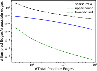
Figure 1: Sparsity ratio of the sampled hypergraphs and bounds.

6.1 Sparsity Ratio Investigation

We first examined if our theoretical bounds in Lemma 3.2 match the actual sparsity ratio in the sampled hyper-graphs. To this end, we followed (Tillinghast and Zhe,, 2021) to sample a series of hyper-graphs with three-way edges (interactions), namely $K=3$. We set $R=1$ and varied $\alpha$ in $[2,20]$. For each particular $\alpha$, we independently sampled $200$ hypergraphs and computed average ratio of the sampled edges. We calculated the bounds accordingly. We show the results in a log-log plot as in Fig. 1. As we can see, the bounds clamp the actual sparsity ratio and match the trend well. The upper bound is tighter. Hence, these bounds can provide a reasonable estimate of the convergence rate and characterize the asymptotic behaviors of the structural sparsity.

6.2 Predictive Performance

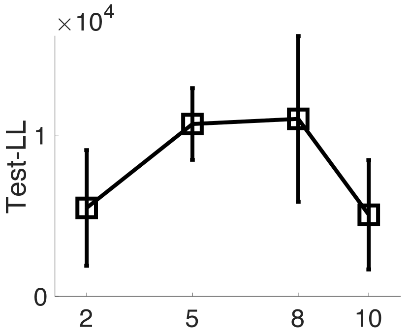
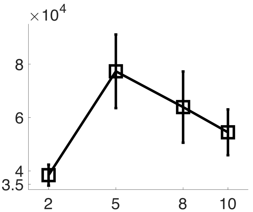
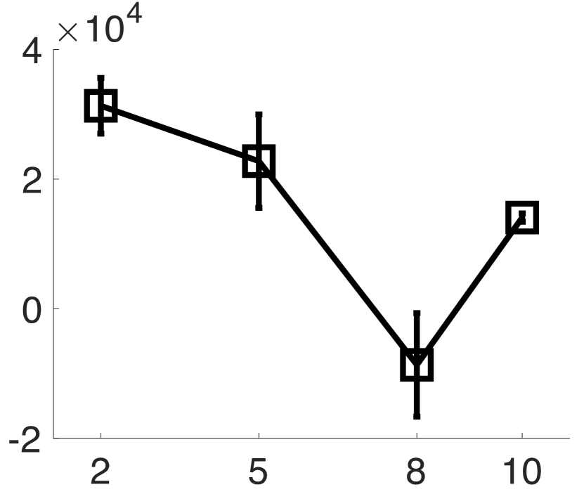
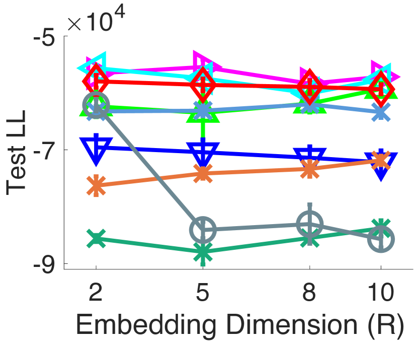
(a) Crash

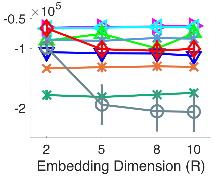
(b) Taobao

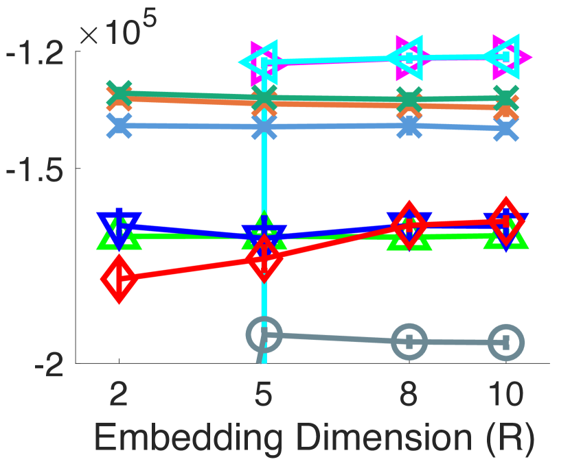
(c) Retail

Figure 2: Test log-likelihood (LL) on real-world datasets. CPT-PTF-{10, 20, 30} means running CPT-PTF with 10, 20 and 30 time steps. The results were averaged over five runs.

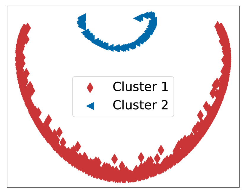
(a) Users

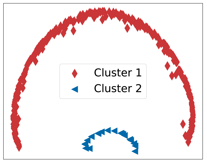
(b) Sellers

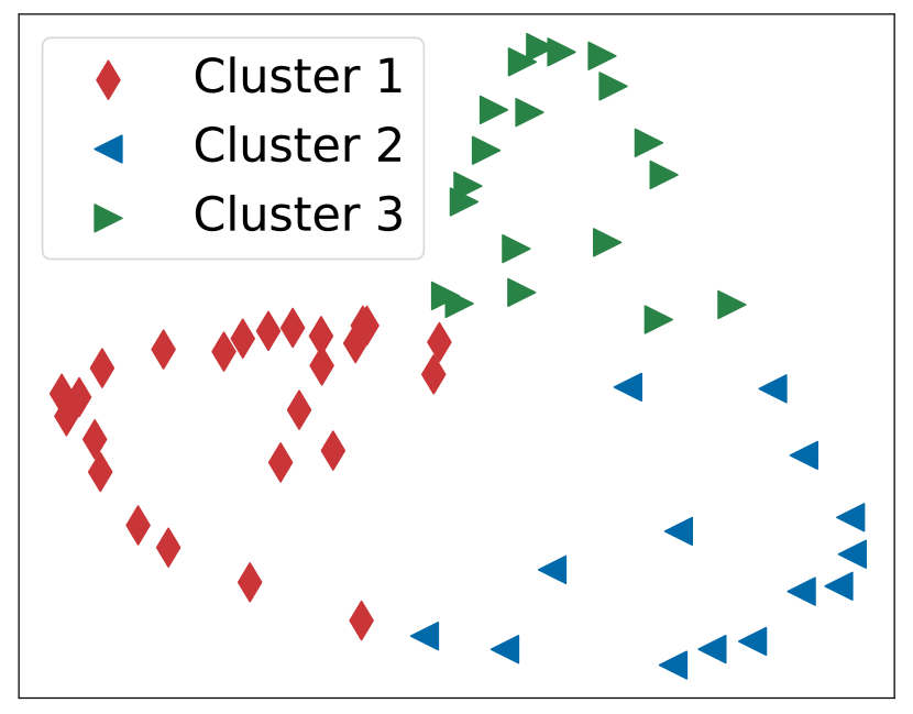
(c) Item Categories

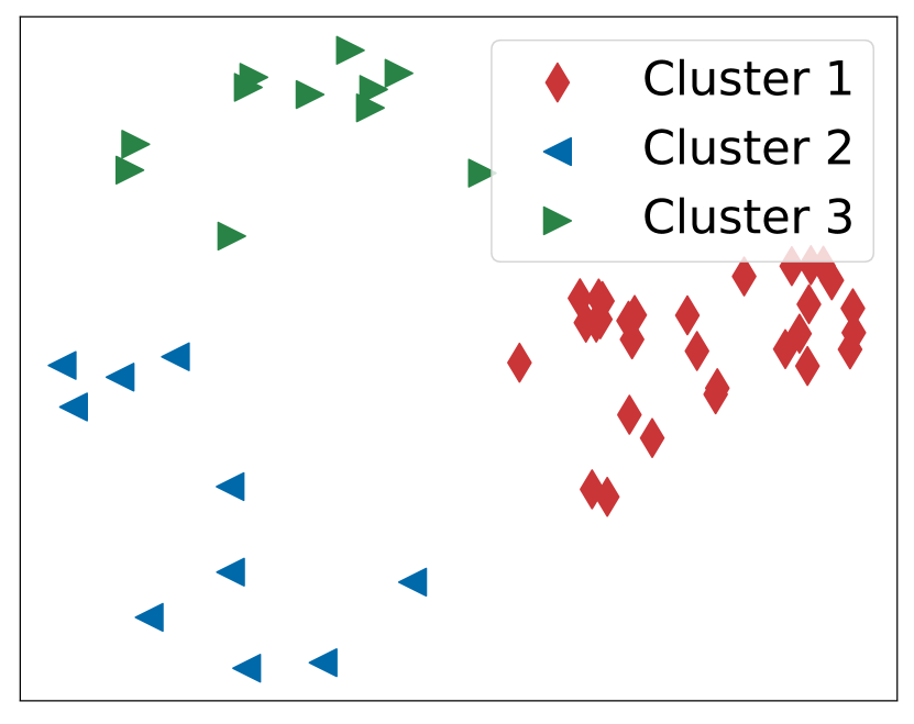
(d) States

Figure 3: Structures of the estimated embeddings on Taobao (a, b, c), Crash (d). The points represent the participant nodes, and the colors indicate their cluster memberships.

Datasets. We then examined the predictive performance of NESH on the following real-world datasets. (1) Taobao (https://tianchi.aliyun.com/dataset/dataDetail?dataId=53), the shopping events in the largest online retail platform of China, from 07/01/2015 to 11/30/2015, which are interactions between $980$ users, $274$ sellers, $631$ items, $58$ categories and $2$ options. There are in total $16,609$ distinct interactions and $69,833$ events. (2) Crash (https://www.kaggle.com/usdot/nhtsa-traffic-fatalities), fatal traffic crashes in US 2015, within $51$ states, $288$ counties, $2,098$ cities and $5$ landuse-types. There are $8,691$ distinct interactions and $32,052$ events in total. (3) Retail (https://tianchi.aliyun.com/dataset/dataDetail?dataId=37260), online retail records from tmall.com. It includes interaction events among stock items and customers. We have $3,310$ and $1,000$ unique items and customers, among which are $31,122$ distinct interactions and $70,000$ events in total. We can see that all these datasets are very sparse. The existent interactions take $0.000085\%$, $0.0056\%$ and $0.94\%$ on Taobao, Crash and Retail, respectively.

Competing Methods. We compared with the following popular and/or state-of-the-art tensor decomposition methods that deal with interaction events. (1) CP-PTF, similar to  (Chi and Kolda,, 2012), the homogeneous Poisson process (PP) tensor decomposition, which uses CP to factorize the event rate for each particular interaction and the square link to ensure the positiveness (consistent with NESH). (2) CPT-PTF, similar to  (Schein et al.,, 2015), which extends CP-PTF by introducing time steps in the tensor. The embeddings of the time steps are assinged a conditional Gaussian prior (Xiong et al.,, 2010) to model their dynamics. (3) GP-PTF, which uses GPs to estimate the square root of of the rate for each particular interaction as a nonlinear function of the associated embeddings. (4) CP-NPTF, non-homogeneous Poisson process tensor factorization where the event rate is modelled as a parametric form, $\lambda_{{\bf i}}(t)=t\cdot\big{(}\mathrm{CP({\bf i})}\big{)}^{2}$. Here $\mathrm{CP}({\bf i})$ is CP decomposition of the entry (interaction) ${\bf i}$. (5) HP-Local (Zhe and Du,, 2018), Hawkes process based decomposition that uses a local time window to model the rate and to estimate the local excitation effects among the nearby events, (6) HP-TF (Pan et al., 2020a, ), another Hawkes process based on factorization method that models both the triggering strength and decay as kernel functions of the embeddings. Both HP-Local and HP-TF use a GP to model the base rate as a function of embeddings. In addition, we compared with (7) MGP-EF, matrix GP based events factorization. It is the same as our method in applying a matrix GP prior over the rates of distinct interactions. However, MGP-EF places a standard Gaussian prior over the embeddings, and so does not model the structure sparsity.

Settings. We implemented NESH, HP-Local, HP-TF and MGP-EF with Pytorch (Paszke et al.,, 2019), and the other methods with MATLAB. For all the approaches employing GPs, we used the same variational approximation as in NESH (our method), and set the number of pseudo inputs to $100$. We used the square exponential (SE) kernel and initialized the kernel parameters with $1$. For HP-Local, the local window size was set to $50$. For our method, we chose $\alpha$ from $\{0.5,1.0,1.5,2.5,3\}$. We conducted stochastic mini-batch optimization for all the methods, where the batch size was set to $100$. We used ADAM (Kingma and Ba,, 2014) algorithm, and the learning rate was tuned from $\{5\times 10^{-4},10^{-3},3\times 10^{-3},5\times 10^{-3},10^{-2}\}$. We ran each method for $400$ epochs, which is enough to converge. We randomly split each dataset into $80\%$ sequences for training, and the remaining $20\%$ for test. We varied $R$, the dimension of the embeddings, from $\{2,5,8,10\}$. For CPT-PTF, we tested the number of time steps from $\{10,20,30\}$. We ran the experiments for five times, and report the average test log-likelihood and its standard deviation in Fig. 2.

Results. As we can see from Fig. 2, NESH consistently outperforms all the competing methods by a large margin. Since the test log-likelihood of NESH is much larger than that of the other methods, we report the result of NESH separately (i.e., in the top figures) so that we can compare the difference between the competing methods. It can be seen that MGP-EF is much better than GP-PTF, implying that introducing a time kernel to model non-homogeneous Poisson process rates is more advantageous. In addition, MGP-EF is much better than or comparable to CP-NPTF (see Fig. 2a). Since both methods uses non-homogeneous Poisson processes, the result demonstrates the advantage of nonparametric rate modeling (the former) over the parametric one (the latter). In most cases, HP-Local and HP-TF shows better or comparable prediction accuracy than MGP-EF. This is reasonable, because the two methods use Hawkes processes that can capture more refined temporal dependencies, i.e., excitation effects between the events. However, both HP-Local and HP-TF cannot capture the sparse structure within the present interactions, and their performance is still much inferior to NESH. Finally, GP-PTF, HP-Local and HP-TF broke down at $R=2$ on Retail dataset. We found their learning was unstable. In some splits, their predictive likelihood are very small, leading to much worse average likelihood than the other methods. Note that they did not use batch normalization as in NESH and MGP-EF, which might cause the learning instability under some settings.

6.3 Pattern Discovery

Next, we examined if NESH can discover hidden patterns from data. To this end, we set $R$ to $5$, and ran NESH on Taobao and Crash. Then we applied kernel PCA (Schölkopf et al.,, 1998) with the SE kernel to project the embeddings onto a plane. We then ran clustering algorithms to find potential structures. As we can see from Fig. 3 a and b, the embeddings of users and items from Taobao dataset exhibit interesting and clear cluster structures, which might correspond to separate interests/shopping habits. Note that we ran DBSCAN (Ester et al.,, 1996) rather than k-means to obtain the clusters. In addition, the embeddings of item categories on Taobao also shows a clear structure that was discovered by k-means (see Fig. 3c). Although the Taobao dataset have been completely anynoymized and we cannot investigate the meaning of these clusters, potentially they can be useful for tasks such as marketing (Zhang et al.,, 2017), recommendation (Liu et al.,, 2015; Tran et al.,, 2018) and click-through-rate prediction (Pan et al.,, 2019). In addition, the embeddings of the states from Crash dataset also exhibit clear structures (see Fig. 3d). We have checked the geolocation of these states and found the states grouped together are often neighborhoods. This is reasonable in that neighboring states might bear a resemblance to each other, in traffic regulations (e.g., speed limit), road conditions, driving customs, weather changes. etc. All these might lead to similar or closely related patterns of traffic accident rates.

7 Conclusion

We have presented NESH, a novel nonparametric embedding method for sparse high-order interaction events. Not only can our method estimate the complex temporal relationships between the participants, our model is also able to capture the structural information underlying the observed sparse interactions. Our theoretical bounds enable convergence rate estimate and reveal insights about the asymptotic behaviors of the sparse prior over hypergraphs or tensors. In the future, we will extend our model to more expressive point processes, such as Hawkes processes, and discover more refined temporal patterns.

Appendix

In this section, we provide detailed proof for Lemma 3.2. To make the ideas accessible to a broad audience, we also give a brief introduction to the Lévy-Khintchine formula as well as the intuition behind it. Our introduction includes the Gamma Processes ($\Gamma$Ps), which are used to sample the intensity measures for a sequence of Poisson Point Processes (PPPs) that are used for sparse tensor/hypergraph construction, as a special case. A comprehensive treatment of the related topics can be found in, for instance, (Ken-Iti,, 1999).

Appendix A The Lévy-Khintchine formula

The sparse tensor model introduced in (Tillinghast and Zhe,, 2021) first generates a discrete measure using $\Gamma$Ps, which are a special type of Lévy process. To better understand the process, we take a brief detour to Lévy processes.

A Lévy process $\{X_{t}\}_{t\geq 0}$ is an ${\mathbb{R}}^{d}$-valued random process such that

• $X_{0}=0$ a.s.;

• $X_{t}$ has stationary and independent increments;

• For every $t$, $X_{t}$ is right-continuous and has a well-defined left-limit.

$X_{t}$ is uniquely determined by $X_{1}$, which is an infinitely divisible random variable. Indeed, if the characteristic function (CF) of $X_{1}$ is $\phi(\xi)$, then the CF of $X_{t}$ is $\phi^{t}(\xi)$ for $t\geq 0$. A complete understanding of $\phi(\xi)$ is sufficient to characterize $X_{t}$, and this can be done via the Lévy-Khintchine formula:

Theorem 1 (Lévy-Khintchine).

Let $X$ be an ${\mathbb{R}}^{d}$-valued random variable. $X$ is infinitely divisible if and only if the CF of $X$, $\phi_{X}(\xi):={\mathbb{E}}[e^{i\xi\cdot X}]$, takes the form

$$\phi_{X}(\xi)=\exp\left\{-\Psi(\xi)\right\},$$ (14)

where

$$\Psi(\xi)=i(a\cdot\xi)+\frac{1}{2}\|\sigma\xi\|^{2}+\int_{{\mathbb{R}}^{d}}(1-e^{i\xi\cdot z}+i(\xi\cdot z)\mathbf{1}_{(0,1)})m(dz),$$ (15)

where $m$ is a Borel measure on ${\mathbb{R}}^{d}$ satisfying $m(\{0\})=0$ and $\int_{{\mathbb{R}}^{d}}(1\wedge\|x\|^{2})m(dx)<\infty$. Here $\Psi$ is called the Lévy exponent of $X$.

As a consequence of Theorem 1, we conclude that the CF of every Lévy process $X_{t}$ can be written as

$$\phi_{t}(\xi)={\mathbb{E}}[e^{i\xi\cdot X_{t}}]=\exp\left\{-t\Psi(\xi)\right\},$$

where $\Psi$ is the Lévy exponent of $X_{1}$.

To comprehend the path structure of $X_{t}$ using (15), we appeal to the following facts:

• Addition of a CF’s exponents corresponds to addition of independent random variables (processes);

• The CF of a drifted Brownian motion $W_{t}=-at+\sigma B_{t}$ is $\exp\{-t(i(a\cdot\xi)-\frac{1}{2}\|\sigma\xi\|^{2})\}$;

• The CF of a compound Poisson process with jump parameter $m$ (i.e. a distribution) and rate parameter $\lambda$ (i.e. a Lévy process) is $\exp\{-t\int_{{\mathbb{R}}^{d}}\lambda(1-e^{i\xi\cdot z})m(dz)\}$.

• The CF of a compensated compound Poisson process with jump parameter $m$ (i.e. a distribution) and rate parameter $\lambda$ (i.e. a Lévy process and a martingale) is $\exp\{-t\int_{{\mathbb{R}}^{d}}\lambda(1-e^{i\xi\cdot z}+i(\xi\cdot z))m(dz)\}$.

Let $I_{0}=\{z:\|z\|\geq 1\}$ and $I_{k}=\{z:\|z\|\in[2^{-k-1},2^{-k})\}$ for $k\geq 1$. Rewrite (15) as

$$t\Psi(\xi) =t(i(a\cdot\xi)+\frac{1}{2}\|\sigma\xi\|^{2})+t\int_{I_{0}}m(I_{0})(1-e^{i\xi\cdot z})\frac{m(dz)}{m(I_{0})}$$

$$\ \ \ \ +\sum_{k=1}^{\infty}t\int_{I_{k}}m(I_{k})(1-e^{i\xi\cdot z}+i(\xi\cdot z))\frac{m(dz)}{m(I_{k})},$$ (16)

where the right-hand side corresponds to three independent processes: a drifted Brownian motion, a compound Poisson process, and a series of independent compensated compound Poisson processes. Under the integrability condition on $m$, the last part can be shown to converge using the martingale theory. Moving the drift term (cumulation of the compensated terms; deterministic) in the last part of (16) into the Brownian motion, we decompose $X_{t}$ into two independent processes, a drifted Brownian motion and a pure-jump process (with countably many jumps). This construction is the celebrated Lévy-Itô construction.

To end this section, we give a useful interpretation of compound Poisson processes. A compound Poisson process $Z_{t}$ with jump parameter $m$ and rate parameter $\lambda$ is defined as

$$Z_{t}=\sum_{i=1}^{N_{t}}M_{i},$$

where $M_{i}\stackrel{{\scriptstyle iid}}{{\sim}}m(dx)$ are independent of $N_{t}\sim\text{Poisson}(\lambda)$. Note $\{M_{i}\}_{i\in[N_{t}]}$ follows a PPP with intensity measure $m(dx)$, for fixed $t$, we may also consider $Z_{t}$ as the integration of $x$ against the Poisson random measure on $[0,t]\times{\mathbb{R}}^{d}$.

Appendix B Gamma processes

A Gamma process $X_{t}$ (with shape parameter $\beta$ and rate parameter $\lambda$) is a Lévy Process with

$$X_{t}\sim\Gamma(\beta t,\lambda) t>0.$$

It can be checked that

$${\mathbb{E}}[e^{i\xi X_{t}}]=\left(1-\frac{i\xi}{\lambda}\right)^{\beta t}=\exp\left\{-t\int_{\mathbb{R}}(1-e^{-i\xi x})\frac{\beta e^{-\lambda x}}{x}\mathbf{1}_{(0,\infty)}dx\right\},$$

i.e., the Lévy measure $m$ is

$$m(dx)=\frac{\beta e^{-\lambda x}}{x}\mathbf{1}_{(0,\infty)}dx.$$

For convenience, we set $\beta=\lambda=1$. From $m$ one can deduce the following properties of $X_{t}$:

• By the Lévy-Itô construction, $X_{t}$ is a pure-jump process (i.e. no Brownian part), i.e., $X_{t}$ has countably infinitely many jumps in $(0,t)$;

• We can associate a sample path of $X_{t}$ (up to time $t$) with the following measure:

  $$w_{t}=\sum_{0<s\leq t}\Delta X_{s}\delta_{s} \Delta X_{s}=X_{s}-\lim_{r\to s^{-}}X_{r},$$ (17)

  where the summation is well-defined since there are at most countably many $s$ that $\Delta_{s}>0$. $w_{t}$ is finite thanks to

  $$\int_{{\mathbb{R}}}(1\wedge x)m(dx)<\infty;$$

• The jump sizes of $X_{t}$, $\{\Delta X_{s}\}_{s\in\text{supp}(w_{t})}\subset(0,\infty)$, follows a PPP with intensity measure $m$; see the last paragraph in Section A.

Appendix C Sparse tensor/hypergraph processes

The sparse hypergraph model considered in this paper is a superposition of $R$ independent sparse tensor process introduced in (Tillinghast and Zhe,, 2021). Without loss of generality, we assume $R=1$; the general case can be analyzed similarly. In this case, the sampled entries in the sparse tensor model are obtained as follows: Given $K\geq 2$ and time $\alpha$, we

• Use $K$ i.i.d. Gamma processes, $X^{(1)}_{\alpha},\cdots,X^{(K)}_{\alpha}$, to generate discrete measures $W_{1}^{\alpha},\cdots,W_{K}^{\alpha}$ as in (17). Here we change the notations to be consistent with the ones in the manuscript, with the index $r$ omitted;

• Construct a product measure $M=\prod_{k=1}^{K}W_{k}^{\alpha}$ on $[0,\alpha]^{K}$;

• Take $M$ as the intensity measure to construct a Poisson random measure $T$. In particular, one can take

  $$T=\{Y_{i}\}_{i=1}^{|T|}\stackrel{{\scriptstyle\text{i.i.d.}}}{{\sim}}\frac{M}{M([0,\alpha]^{K})} |T|\sim\text{Poisson}(M([0,\alpha]^{K}))\mathchoice{\mathrel{\hbox to0.0pt{$\displaystyle\perp$\hss}\mkern 2.0mu{\displaystyle\perp}}}{\mathrel{\hbox to0.0pt{$\textstyle\perp$\hss}\mkern 2.0mu{\textstyle\perp}}}{\mathrel{\hbox to0.0pt{$\scriptstyle\perp$\hss}\mkern 2.0mu{\scriptstyle\perp}}}{\mathrel{\hbox to0.0pt{$\scriptscriptstyle\perp$\hss}\mkern 2.0mu{\scriptscriptstyle\perp}}}Y_{i},$$ (18)

  where $X\mathchoice{\mathrel{\hbox to0.0pt{$\displaystyle\perp$\hss}\mkern 2.0mu{\displaystyle\perp}}}{\mathrel{\hbox to0.0pt{$\textstyle\perp$\hss}\mkern 2.0mu{\textstyle\perp}}}{\mathrel{\hbox to0.0pt{$\scriptstyle\perp$\hss}\mkern 2.0mu{\scriptstyle\perp}}}{\mathrel{\hbox to0.0pt{$\scriptscriptstyle\perp$\hss}\mkern 2.0mu{\scriptscriptstyle\perp}}}Y$ means that $X$ and $Y$ are independent. The support of $T$ corresponds to sampled entries in the sparse tensor, and the marginals of the support of $T$ corresponds to the size of the sparse tensor in the respective dimension.

To get an explicit rate of convergence of sparsity as $\alpha\to\infty$, we need to estimate the cardinality of the support of $T$, $N^{\alpha}$, as well as of the corresponding marginals, which are denoted by $D_{1}^{\alpha},\cdots,D_{K}^{\alpha}$.

Lemma 2.

Fix $K\geq 2$. For a sparse tensor process defined as above, for all sufficiently large $\alpha$, there exists an absolute constant $C>0$ such that, with probability at least $1-(C\alpha)^{-K}$,

$$\frac{e^{-1.03(2K)^{1/K}K(\log\alpha)^{1/K}}}{2K\log\alpha}\cdot\left[\frac{1.82}{(K-1)\log(1.01\alpha)}\right]^{K}\leq\frac{N^{\alpha}}{\prod_{k=1}^{K}D_{k}^{\alpha}}\leq\left[\frac{2.11}{(K-1)\log(0.99\alpha)}\right]^{K}.$$

Proof.

Analysis of $N^{\alpha}$. We begin by deriving an upper bound for $N^{\alpha}$. Note $N^{\alpha}\leq|T|$, where the $|T|$ is defined in (18). Conditioned on $M$,

$$|T|\sim\text{Poisson}(\gamma_{\alpha}) \gamma_{\alpha}=M([0,\alpha]^{K})=\prod_{k=1}^{K}W_{k}^{\alpha}([0,\alpha]).$$

By a Poisson tail estimate (Vershynin,, 2018, Exercise 2.3.6), we have

$${\mathbb{P}}\left(0.99\gamma_{\alpha}\leq|T|\leq 1.01\gamma_{\alpha}\right)\geq 1-2e^{-c_{1}\gamma_{\alpha}},$$ (19)

where $c_{1}>0$ is an absolute constant. For each $k\in[K]$,

$$W_{k}^{\alpha}([0,\alpha])\stackrel{{\scriptstyle\eqref{gamma-measure}}}{{=}}\sum_{0<s\leq\alpha}\Delta X^{(k)}_{s}=X^{(k)}_{\alpha}\sim\Gamma(\alpha,1).$$

Without loss of generality, we assume $\alpha\in{\mathbb{N}}$ (otherwise consider $\lceil\alpha\rceil$ and $\lfloor\alpha\rfloor$). Then, we can write $X^{(k)}_{\alpha}$ as a sum of i.i.d. exponentials with unit rate:

$$X^{(k)}_{\alpha}\stackrel{{\scriptstyle\mathcal{D}}}{{=}}\sum_{i=1}^{\alpha}G_{i} G_{i}\stackrel{{\scriptstyle\text{i.i.d.}}}{{\sim}}\text{Exp}(1),$$

where $\text{Exp}(1)$ is the exponential random variable with unit rate. An application of Bernstein’s inequality yields

$${\mathbb{P}}\left(0.99\alpha\leq W_{k}^{\alpha}([0,\alpha])\leq 1.01\alpha\right)\geq 1-2e^{-c_{2}\alpha},$$

where $c_{2}>0$ is an absolute constant (depending only on $\beta$ and $\lambda$ both of which are equal to $1$). Taking a union bound over $k$ yields

$${\mathbb{P}}\left(0.99\alpha\leq\min_{k}W_{k}^{\alpha}([0,\alpha])\leq\max_{k}W_{k}^{\alpha}([0,\alpha])\leq 1.01\alpha\right)\geq 1-2Ke^{-c_{2}\alpha}.$$ (20)

Combining (19) and (20) via a union bound yields that, with probability at least $1-2e^{-c_{1}(0.99\alpha)^{K}}-2Ke^{-c_{2}\alpha}$,

$$N^{\alpha}\leq|T|\leq 1.01^{K+1}\alpha^{K} |T|\geq 0.99^{K+1}\alpha^{K}.$$ (21)

A lower bound on $N^{\alpha}$ requires more refined analysis. Let

$$a=\frac{1.01}{0.99^{\frac{K+1}{K}}}(2K\log\alpha)^{1/K}\leq 1.03(2K\log\alpha)^{1/K} K\geq 2.$$ (22)

For all sufficiently large $\alpha$, $1\leq a\to\infty$, and

$$\alpha\cdot m([a,\infty)) \leq\alpha\cdot m([1,\infty))=\alpha\int_{1}^{\infty}\frac{e^{-x}}{x}dx\leq\alpha\int_{1}^{\infty}e^{-x}dx\leq\alpha$$ (23)

$$\alpha\cdot m([a,\infty)) \geq\alpha\cdot m([a,1.01a))=\alpha\int_{a}^{1.01a}\frac{e^{-x}}{x}dx$$

$$\geq\alpha\int_{a}^{1.01a}\frac{e^{-x}}{1.01a}dx=\frac{\alpha e^{-a}\left(1-e^{-0.01a}\right)}{1.01a}\geq\frac{0.99\alpha e^{-a}}{a}\geq\sqrt{\alpha}.$$ (24)

In this case, a similar Poisson tail estimate as before yields

$${\mathbb{P}}\left(0.99\alpha m([a,\infty))\leq\min_{k}\#\{s\leq\alpha:\Delta X^{(k)}_{s}\in[a,\infty)\}\leq\max_{k}\#\{s\leq\alpha:\Delta X^{(k)}_{s}\in[a,\infty)\}\leq 1.01\alpha m([a,\infty))\right)$$

$$\stackrel{{\scriptstyle\eqref{hhh}}}{{\geq}} \ 1-2Ke^{-c_{1}\sqrt{\alpha}}.$$ (25)

Conditioning $M$ and $|T|$ on the intersection of the events in (20), (21) and (25), we write

$$N^{\alpha}=\sum_{s=(s_{1},\cdots,s_{K})\in\text{supp}(M)}\mathbf{1}_{s\in T}\geq\sum_{s\in\mathcal{S}}\mathbf{1}_{s\in T},$$ (26)

where

$$\mathcal{S}=\left\{s=(s_{1},\cdots,s_{K})\in\text{supp}(M):\Delta X_{s_{k}}^{(k)}\geq a,\;\forall k\in[K]\right\}.$$

Each term in the summand in the right-hand side of (26) is a Bernoulli random variable with parameter

$$p_{s}:=1-\left(1-\frac{\prod_{k=1}^{K}\Delta X^{(k)}_{s_{k}}}{M([0,\alpha]^{K})}\right)^{|T|} \stackrel{{\scriptstyle\eqref{002},\eqref{re1}}}{{\geq}}1-\left[1-\left(\frac{a}{1.01\alpha}\right)^{K}\right]^{0.99^{K+1}\alpha^{K}}$$

$$=1-\left(1-\frac{2K\log\alpha}{0.99^{K+1}\alpha^{K}}\right)^{0.99^{K+1}\alpha^{K}}\geq 1-\alpha^{-2K},$$ (27)

where the last step used the fact that $(1-\frac{1}{x})^{x}\leq e^{-1}$ for $x>1$. In particular, for $s\in\mathcal{S}$,

$${\mathbb{P}}\left(\mathbf{1}_{s\in T}=0\right)=1-p_{s}\stackrel{{\scriptstyle\eqref{lalaba}}}{{\leq}}\alpha^{-2K}.$$ (28)

Since

$$\frac{0.95^{K}(\alpha e^{-1.03(2K)^{1/K}(\log\alpha)^{1/K}})^{K}}{2K\log\alpha}\stackrel{{\scriptstyle\eqref{zsa}}}{{\leq}}0.99^{2K}\left(\frac{\alpha e^{-a}}{a}\right)^{K}\stackrel{{\scriptstyle\eqref{hhh},\eqref{ggg}}}{{\leq}}|\mathcal{S}|\stackrel{{\scriptstyle\eqref{hhhh},\eqref{ggg}}}{{\leq}}1.01^{K}\alpha^{K},$$ (29)

taking a union bound over $s\in\mathcal{S}$ yields that, with probability at least

$$1-2e^{-c_{1}(0.99\alpha)^{K}}-2Ke^{-c_{2}\alpha}-2Ke^{-c_{3}\alpha}-2Ke^{-c_{1}\sqrt{\alpha}}-\sum_{s\in\mathcal{S}}(1-p_{s})$$

$$\stackrel{{\scriptstyle\eqref{zzzz},\eqref{zzz}}}{{\geq}} \ 1-2e^{-c_{1}(0.99\alpha)^{K}}-2Ke^{-c_{2}\alpha}-2Ke^{-c_{3}\alpha}-2Ke^{-c_{1}\sqrt{\alpha}}-1.01^{K}\alpha^{-K},$$

the following holds:

$$N^{\alpha}\geq|\mathcal{S}|\geq\frac{0.95^{K}(\alpha e^{-1.03(2K)^{1/K}(\log\alpha)^{1/K}})^{K}}{2K\log\alpha}.$$ (30)

Analysis of $D_{k}^{\alpha}$. Analysis of $D_{k}^{\alpha}$ is easy owing to an observation in (Tillinghast and Zhe,, 2021): For $k\in[K]$, conditioned on $W_{\ell}^{\alpha}$, $\ell\neq k$,

$$D_{k}^{\alpha}\sim\text{Poisson}\left(\alpha\psi\left(\gamma_{\alpha}^{(-k)}\right)\right),$$

where

$$\gamma_{\alpha}^{(-k)}=\prod_{\ell\neq k}W_{k}^{\alpha}([0,\alpha]) \psi(\alpha)=\int_{\mathbb{R}}(1-e^{-\alpha x})m(dx).$$

By a similar Poisson tail estimate as before,

$${\mathbb{P}}\left(0.99\alpha\psi(\gamma_{\alpha}^{(-k)})\leq D_{k}^{\alpha}\leq 1.01\alpha\psi(\gamma_{\alpha}^{(-k)})\right)\geq 1-2e^{-c_{1}\alpha\psi(\gamma_{\alpha}^{(-k)})}.$$ (31)

It is easy to check via L’Hôpital’s rule that

$$\lim_{\alpha\to\infty}\frac{\psi(\alpha)}{\log\alpha}=\lim_{\alpha\to\infty}\alpha\frac{d}{d\alpha}\psi(\alpha)=\lim_{\alpha\to\infty}\alpha\int_{\mathbb{R}}xe^{-\alpha x}(1-e^{-\alpha x})m(dx)=\lim_{\alpha\to\infty}\frac{\alpha^{2}}{(\alpha+1)(2\alpha+1)}=\frac{1}{2}.$$

Hence, for all sufficiently large $\alpha$,

$$0.49\log\alpha\leq\psi(\alpha)\leq 0.51\log\alpha.$$ (32)

Thus, conditioned on the event $0.99\alpha\leq\min_{\ell\neq k}W_{\ell}^{\alpha}([0,\alpha])\leq\max_{\ell\neq k}W^{\alpha}_{\ell}([0,\alpha])\leq 1.01\alpha$ (which holds with probability at least as the lower bound in (20)), (31) and (32) together implies that, for all sufficiently large $\alpha$,

$${\mathbb{P}}\left(0.48(K-1)\alpha\log\left(0.99\alpha\right)\leq D_{k}^{\alpha}\leq 0.52(K-1)\alpha\log\left(1.01\alpha\right)\right)\geq 1-2e^{-c_{1}(0.99\alpha)^{K}}.$$

Taking a union bound over $k$ yields that, for all sufficiently large $\alpha$, with probability at least $1-2Ke^{-c_{1}(0.99\alpha)^{K}}$,

$$0.48(K-1)\alpha\log\left(0.99\alpha\right)\leq\min_{k}D_{k}^{\alpha}\leq\max_{k}D_{k}^{\alpha}\leq 0.52(K-1)\alpha\log\left(1.01\alpha\right).$$ (33)

Combining (21), (30), (33) and renaming the constants yields the desired result. ∎

References

- Brix, (1999) Brix, A. (1999). Generalized gamma measures and shot-noise cox processes. Advances in Applied Probability, pages 929–953.
- Caron and Fox, (2014) Caron, F. and Fox, E. B. (2014). Sparse graphs using exchangeable random measures. arXiv preprint arXiv:1401.1137.
- Caron and Fox, (2017) Caron, F. and Fox, E. B. (2017). Sparse graphs using exchangeable random measures. Journal of the Royal Statistical Society. Series B, Statistical Methodology, 79(5):1295.
- Chi and Kolda, (2012) Chi, E. C. and Kolda, T. G. (2012). On tensors, sparsity, and nonnegative factorizations. SIAM Journal on Matrix Analysis and Applications, 33(4):1272–1299.
- Choi and Vishwanathan, (2014) Choi, J. H. and Vishwanathan, S. (2014). Dfacto: Distributed factorization of tensors. In Advances in Neural Information Processing Systems, pages 1296–1304.
- Chu and Ghahramani, (2009) Chu, W. and Ghahramani, Z. (2009). Probabilistic models for incomplete multi-dimensional arrays. AISTATS.
- Du et al., (2018) Du, Y., Zheng, Y., Lee, K.-c., and Zhe, S. (2018). Probabilistic streaming tensor decomposition. In 2018 IEEE International Conference on Data Mining (ICDM), pages 99–108. IEEE.
- Engen, (1975) Engen, S. (1975). A note on the geometric series as a species frequency model. Biometrika, 62(3):697–699.
- Ester et al., (1996) Ester, M., Kriegel, H.-P., Sander, J., and Xu, X. (1996). A density-based algorithm for discovering clusters in large spatial databases with noise. In Kdd, volume 96, pages 226–231.
- (10) Fang, S., Kirby, R. M., and Zhe, S. (2021a). Bayesian streaming sparse Tucker decomposition. In Uncertainty in Artificial Intelligence, pages 558–567. PMLR.
- (11) Fang, S., Wang, Z., Pan, Z., Liu, J., and Zhe, S. (2021b). Streaming Bayesian deep tensor factorization. In International Conference on Machine Learning, pages 3133–3142. PMLR.
- Ferguson, (1973) Ferguson, T. S. (1973). A Bayesian analysis of some nonparametric problems. The annals of statistics, pages 209–230.
- Griffiths, (1980) Griffiths, R. C. (1980). Lines of descent in the diffusion approximation of neutral wright-fisher models. Theoretical population biology, 17(1):37–50.
- Hansen et al., (2015) Hansen, S., Plantenga, T., and Kolda, T. G. (2015). Newton-based optimization for Kullback-Leibler nonnegative tensor factorizations. Optimization Methods and Software, 30(5):1002–1029.
- Harshman, (1970) Harshman, R. A. (1970). Foundations of the PARAFAC procedure: Model and conditions for an”explanatory”multi-mode factor analysis. UCLA Working Papers in Phonetics, 16:1–84.
- Hensman et al., (2013) Hensman, J., Fusi, N., and Lawrence, N. D. (2013). Gaussian processes for big data. In Proceedings of the Twenty-Ninth Conference on Uncertainty in Artificial Intelligence, pages 282–290. AUAI Press.
- Hougaard, (1986) Hougaard, P. (1986). Survival models for heterogeneous populations derived from stable distributions. Biometrika, 73(2):387–396.
- (18) Hu, C., Rai, P., and Carin, L. (2015a). Zero-truncated poisson tensor factorization for massive binary tensors. In UAI.
- (19) Hu, C., Rai, P., Chen, C., Harding, M., and Carin, L. (2015b). Scalable bayesian non-negative tensor factorization for massive count data. In Proceedings, Part II, of the European Conference on Machine Learning and Knowledge Discovery in Databases - Volume 9285, ECML PKDD 2015, pages 53–70, New York, NY, USA. Springer-Verlag New York, Inc.
- Ioffe and Szegedy, (2015) Ioffe, S. and Szegedy, C. (2015). Batch normalization: Accelerating deep network training by reducing internal covariate shift. In International conference on machine learning, pages 448–456. PMLR.
- Kang et al., (2012) Kang, U., Papalexakis, E., Harpale, A., and Faloutsos, C. (2012). Gigatensor: scaling tensor analysis up by 100 times-algorithms and discoveries. In Proceedings of the 18th ACM SIGKDD international conference on Knowledge discovery and data mining, pages 316–324. ACM.
- Ken-Iti, (1999) Ken-Iti, S. (1999). Lévy processes and infinitely divisible distributions. Cambridge university press.
- Kingma and Ba, (2014) Kingma, D. P. and Ba, J. (2014). Adam: A method for stochastic optimization. arXiv preprint arXiv:1412.6980.
- Kingma and Welling, (2013) Kingma, D. P. and Welling, M. (2013). Auto-encoding variational bayes. arXiv preprint arXiv:1312.6114.
- Kingman, (1967) Kingman, J. (1967). Completely random measures. Pacific Journal of Mathematics, 21(1):59–78.
- Kingman, (1992) Kingman, J. (1992). Poisson Processes, volume 3. Clarendon Press.
- Kolda, (2006) Kolda, T. G. (2006). Multilinear operators for higher-order decompositions, volume 2. United States. Department of Energy.
- Kolda and Bader, (2009) Kolda, T. G. and Bader, B. W. (2009). Tensor decompositions and applications. SIAM Review, 51(3):455–500.
- Lijoi et al., (2010) Lijoi, A., Prünster, I., et al. (2010). Models beyond the Dirichlet process. Bayesian nonparametrics, 28(80):342.
- Liu et al., (2018) Liu, B., He, L., Li, Y., Zhe, S., and Xu, Z. (2018). Neuralcp: Bayesian multiway data analysis with neural tensor decomposition. Cognitive Computation, 10(6):1051–1061.
- Liu et al., (2015) Liu, Y.-F., Hsu, C.-Y., and Wu, S.-H. (2015). Non-linear cross-domain collaborative filtering via hyper-structure transfer. In International Conference on Machine Learning, pages 1190–1198. PMLR.
- Lloyd et al., (2015) Lloyd, C., Gunter, T., Osborne, M., and Roberts, S. (2015). Variational inference for gaussian process modulated poisson processes. In International Conference on Machine Learning, pages 1814–1822. PMLR.
- McCloskey, (1965) McCloskey, J. W. (1965). A model for the distribution of individuals by species in an environment. Michigan State University. Department of Statistics.
- Pan et al., (2019) Pan, F., Li, S., Ao, X., Tang, P., and He, Q. (2019). Warm up cold-start advertisements: Improving ctr predictions via learning to learn id embeddings. In Proceedings of the 42nd International ACM SIGIR Conference on Research and Development in Information Retrieval, pages 695–704.
- Pan et al., (2021) Pan, Z., Wang, Z., Phillips, J. M., and Zhe, S. (2021). Self-adaptable point processes with nonparametric time decays. Advances in Neural Information Processing Systems, 34.
- (36) Pan, Z., Wang, Z., and Zhe, S. (2020a). Scalable nonparametric factorization for high-order interaction events. In International Conference on Artificial Intelligence and Statistics, pages 4325–4335. PMLR.
- (37) Pan, Z., Wang, Z., and Zhe, S. (2020b). Streaming nonlinear Bayesian tensor decomposition. In Conference on Uncertainty in Artificial Intelligence, pages 490–499. PMLR.
- Paszke et al., (2019) Paszke, A., Gross, S., Massa, F., Lerer, A., Bradbury, J., Chanan, G., Killeen, T., Lin, Z., Gimelshein, N., Antiga, L., et al. (2019). Pytorch: An imperative style, high-performance deep learning library. In NeurIPS.
- Rai et al., (2014) Rai, P., Wang, Y., Guo, S., Chen, G., Dunson, D., and Carin, L. (2014). Scalable Bayesian low-rank decomposition of incomplete multiway tensors. In Proceedings of the 31th International Conference on Machine Learning (ICML).
- Rasmussen and Williams, (2006) Rasmussen, C. E. and Williams, C. K. I. (2006). Gaussian Processes for Machine Learning. MIT Press.
- Schein et al., (2019) Schein, A., Linderman, S. W., Zhou, M., Blei, D. M., and Wallach, H. M. (2019). Poisson-randomized gamma dynamical systems. In NeurIPS.
- Schein et al., (2015) Schein, A., Paisley, J., Blei, D. M., and Wallach, H. (2015). Bayesian poisson tensor factorization for inferring multilateral relations from sparse dyadic event counts. In Proceedings of the 21th ACM SIGKDD International Conference on Knowledge Discovery and Data Mining, pages 1045–1054. ACM.
- Schein et al., (2016) Schein, A., Zhou, M., Blei, D. M., and Wallach, H. (2016). Bayesian poisson tucker decomposition for learning the structure of international relations. In Proceedings of the 33rd International Conference on International Conference on Machine Learning - Volume 48, ICML’16, pages 2810–2819. JMLR.org.
- Schölkopf et al., (1998) Schölkopf, B., Smola, A., and Müller, K.-R. (1998). Nonlinear component analysis as a kernel eigenvalue problem. Neural computation, 10(5):1299–1319.
- Sethuraman, (1994) Sethuraman, J. (1994). A constructive definition of dirichlet priors. Statistica sinica, pages 639–650.
- Tillinghast et al., (2020) Tillinghast, C., Fang, S., Zhang, K., and Zhe, S. (2020). Probabilistic neural-kernel tensor decomposition. In 2020 IEEE International Conference on Data Mining (ICDM), pages 531–540. IEEE.
- Tillinghast and Zhe, (2021) Tillinghast, C. and Zhe, S. (2021). Nonparametric decomposition of sparse tensors. In International Conference on Machine Learning, pages 10301–10311. PMLR.
- Titsias, (2009) Titsias, M. K. (2009). Variational learning of inducing variables in sparse gaussian processes. In International Conference on Artificial Intelligence and Statistics, pages 567–574.
- Tran et al., (2018) Tran, T., Lee, K., Liao, Y., and Lee, D. (2018). Regularizing matrix factorization with user and item embeddings for recommendation. In Proceedings of the 27th ACM International Conference on Information and Knowledge Management, pages 687–696.
- Tucker, (1966) Tucker, L. (1966). Some mathematical notes on three-mode factor analysis. Psychometrika, 31:279–311.
- Vershynin, (2018) Vershynin, R. (2018). High-dimensional probability: An introduction with applications in data science, volume 47. Cambridge university press.
- Wang et al., (2020) Wang, Z., Chu, X., and Zhe, S. (2020). Self-modulating nonparametric event-tensor factorization. In International Conference on Machine Learning, pages 9857–9867. PMLR.
- Williamson, (2016) Williamson, S. A. (2016). Nonparametric network models for link prediction. The Journal of Machine Learning Research, 17(1):7102–7121.
- Xiong et al., (2010) Xiong, L., Chen, X., Huang, T.-K., Schneider, J., and Carbonell, J. G. (2010). Temporal collaborative filtering with bayesian probabilistic tensor factorization. In Proceedings of the 2010 SIAM International Conference on Data Mining, pages 211–222. SIAM.
- Yang and Dunson, (2013) Yang, Y. and Dunson, D. (2013). Bayesian conditional tensor factorizations for high-dimensional classification. Journal of the Royal Statistical Society B, revision submitted.
- Zhang et al., (2017) Zhang, C., Phang, C. W., Wu, Q., and Luo, X. (2017). Nonlinear effects of social connections and interactions on individual goal attainment and spending: Evidences from online gaming markets. Journal of Marketing, 81(6):132–155.
- Zhao et al., (2015) Zhao, Q., Zhang, L., and Cichocki, A. (2015). Bayesian cp factorization of incomplete tensors with automatic rank determination. IEEE transactions on pattern analysis and machine intelligence, 37(9):1751–1763.
- Zhe and Du, (2018) Zhe, S. and Du, Y. (2018). Stochastic nonparametric event-tensor decomposition. In Advances in Neural Information Processing Systems, pages 6856–6866.
- (59) Zhe, S., Qi, Y., Park, Y., Xu, Z., Molloy, I., and Chari, S. (2016a). Dintucker: Scaling up Gaussian process models on large multidimensional arrays. In Thirtieth AAAI conference on artificial intelligence.
- Zhe et al., (2015) Zhe, S., Xu, Z., Chu, X., Qi, Y., and Park, Y. (2015). Scalable nonparametric multiway data analysis. In Proceedings of the Eighteenth International Conference on Artificial Intelligence and Statistics, pages 1125–1134.
- (61) Zhe, S., Zhang, K., Wang, P., Lee, K.-c., Xu, Z., Qi, Y., and Ghahramani, Z. (2016b). Distributed flexible nonlinear tensor factorization. In Advances in Neural Information Processing Systems, pages 928–936.