Acknowledgment

5

Hongkang Li

Rensselaer Polytechnic Institute

Dr. Shuai Zhang

Rensselaer Polytechnic Institute

Dr. Sijia Liu

Michigan State University

Dr. Pin-Yu Chen

IBM Research

Dr. Jinjun Xiong

University at Buffalo These works were supported by AFOSR, ARO, NSF and the Rensselaer-IBM AI Research Collaboration.

Deep Neural Networks

.4

Figure 1: *

Computer Vision

Figure 2: *

Recommendation System

.4

Figure 3: *

Natural Language Processing

Figure 4: *

Gaming

Great empirical success, but limited theoretical justification.

Generalization Analysis of Neural Networks

Why does the model learned by minimizing the empirical risk on the training data perform well on the testing data? [t].45 Challenges for training performance Non-convex objective function
Challenges for small generalization gap Insufficient training samples [t].4

Figure 5: *

Training and test error against the number of samples

To guarantee the testing performance, need a small training error and a small generalization gap simultaneously.

Related Works on Generalization Analysis

Overparameterized neural networks

number of learnable parameters ¿ number of training samples [t].45 Pros

1. Allow random initialization.

2. Zero training error.

[t].45 Cons

1. Consider linearized networks $\rightarrow$ The training problem is convex.

2. Do not explain the advantage of deep networks.

3. Require a significantly larger number of neurons than that in practice.
   

• Mean Field: [Mei et al., 2018; Chizat & Bach, 2018; Fang et al., 2019; Nguyen, 2019]

• Neural Tangent Kernel: [Jacot et al., 2018; Allen-Zhu et al., 2019; Du et al, 2019; Zou et al., 2019; 2020].

Related works

Model recovery framework [t] .6

• Assume a fixed network with unknown ground-truth parameter $\bfW^{*}$. The output $y$ is generated by $\bfW^{*}$ and the input $\bfx\in\mathbb{R}^{d}$. We aim to estimate $\bfW^{*}$ given dataset $\{\bfx_{i},y_{i}\}_{i=1}^{n}$.

• Generalization error of a returned model $\bfW$ is measured by $\|\bfW-\bfW^{*}\|_{F}$.

• Solves the nonlinear the empirical risk minimization directly.

  • Landscape analysis: almost locally convex near $\bfW^{*}$

  • Initialize near $\bfW^{*}$ followed by gradient descent.

This line of works includes [Zhong et al., 2017; Zhang et al., 2020a; 2020b; 2021a; 2021b; Fu et al., 2020]. .4

Figure 6: *

Objective function and population risk function

Related works

Pros

1. Deal with the network with a fixed number of neurons.

2. No linearization of the network.
   

Cons

1. One-hidden-layer neural networks

2. Input from the standard Gaussian with zero mean and unit variance.

Gaussian Mixture Model

• Generalization analysis of neural networks with non-standard Gaussian inputs is less investigated.

• Many practical datasets can be modelled by a mixture of distributions [Li & Liang, 2018].

• We formulate a Gaussian mixture model (GMM) as the input distribution.

.35

Figure 7: *

MNIST [LeCun et al., 1998]

.35

Figure 8: *

Cifar-10 [Krizhevsky, 2009]

.35

Figure 9: *

ImageNet [Deng et al., 2009]

Q: what is the generalization guarantee when data follow GMM?
How does the mean and variance affect the learning performance?

Problem Formulation

[t] .65

• Input data following GMM: $\bfx\sim\sum_{l=1}^{L}\lambda_{l}\mathcal{N}(\boldsymbol{\mu}_{l},\boldsymbol{\Sigma}_{l})\in\mathcal{R}^{d}$
  

• One-hidden-layer network with ground-truth weights $\bfW^{*}$.

  $$\mathbb{P}(y=1|\bfx)=\frac{1}{K}\sum_{j=1}^{K}\phi({\bfw_{j}^{*}}^{\top}\bfx)$$ (1)

  $\phi$ is the sigmoid function.

• Given $n$ pairs of data $\{\bfx_{i},y_{i}\}_{i=1}^{n}$, the training problem minimizes the empirical loss

  $$f_{n}(\bfW)=\frac{1}{n}\sum_{i=1}^{n}\ell(\bfW;\bfx_{i},y_{i}),$$ (2)

  where $\ell$ is the cross-entropy function.

.35

Figure 10: *

One-hidden-layer networks

Algorithm

[t] .45

[H] *Gradient Descent with Tensor Initialization [1] Input: Training data $\{(\bfx_{i},y_{i})\}_{i=1}^{n}$, the step size $\eta_{0}$; Initialization: $\bfW_{0}\leftarrow$ Tensor initialization method; $t=0,1,\cdots,T-1$ $\bfW_{t+1}=\bfW_{t}-\eta_{0}\nabla f_{n}(\bfW)$ Output: $\bfW_{T}$ .45 Tensor Initialization

• Initialize a weight matrix in the local convex region of $\bfW^{*}$.

• We develop a different tensor construction from that in [Zhong et al., 2017] because of the non-standard-Gaussian input.

Vanilla Gradient Descent

Main Theoretical Results

Given the samples from $\{\bfx_{i},y_{i}\}_{i=1}^{n}$ satisfying

$$n\geq n_{\textrm{sc}}:=poly(K)\mathcal{B}\cdot d\log^{2}{d}$$ (3)

for positive value functions $\mathcal{B}$ and $v$ with high probability, the iterates $\{\bfW_{t}\}_{t=1}^{T}$ returned by Algorithm 1 converge linearly to a critical point $\widehat{\bfW}_{n}$ with the rate of convergence $v$, i.e.,

$$||\bfW_{t}-\widehat{\bfW}_{n}||_{F}\leq v^{t}||\bfW_{0}-\widehat{\bfW}_{n}||_{F}.$$ (4)

There exists a permutation matrix $\bfP^{*}$ such that the distance between $\widehat{\bfW}_{n}$ and $\bfW^{*}\bfP^{*}$ is

$$||\widehat{\bfW}_{n}-\bfW^{*}\bfP^{*}||_{F}\leq O\Big{(}K^{\frac{5}{2}}\cdot\sqrt{d\log{n}/n}\Big{)}.$$ (5)

Main Theoretical Results (cont’d)

When everything else is fixed,

1. $n_{sc}$ and $v$ increase as the norm of one mean increases.

2. $n_{sc}$ and $v$ first decreases and then increases, as the norm of one covariance matrix increases,

• Sample complexity: $\Theta(d\log^{2}d)$, the same order as the case of standard Gaussian inputs in [Zhong et al., 2017; Fu et al., 2020].

• The iterates converge to $\widehat{\bfW}_{n}$ linearly. $\widehat{\bfW}_{n}$ is close to $\bfW^{*}$ with a diminishing distance in $n$.

• Mean increases $\rightarrow$ a higher sample complexity and converges slower.

• Variance increase $\rightarrow$ the sample complexity first decreases and then increases; converges faster first and then slower.

Technical challenges

1. Landscape analysis fails with non-standard-Gaussian inputs

   • We show the local strong convexity around $\bfW^{*}$.
     

2. Generalization gap bound is required for the new input distribution

   • We establish new concentration bounds.
     

3. The initialization method needs to be updated.

   • We develop a new version of tensor initialization with new tensor constructions.

Empirical experiments

Settings

• $d=5$.

• Generate $\bfW^{*}$ with each entry from $\mathcal{N}(0,1)$.

• Initialize $\bfW_{0}$ close to $\bfW^{*}$.
  

GMM

1. Sample complexity against feature dimension.

   • $\bfx\sim\frac{1}{2}\mathcal{N}(\boldsymbol{1},\bfI)+\frac{1}{2}\mathcal{N}(-\boldsymbol{1},\bfI)$.

2. Sample complexity/Convergence rate against mean value.

   • $\bfx\sim\frac{1}{2}\mathcal{N}(\mu\cdot\boldsymbol{1},\bfI)+\frac{1}{2}\mathcal{N}(-\mu\cdot\boldsymbol{1},\bfI)$.

3. Sample complexity/Convergence rate against variance value.

   • $\bfx\sim\frac{1}{2}\mathcal{N}(\boldsymbol{1},\boldsymbol{\Sigma})+\frac{1}{2}\mathcal{N}(-\boldsymbol{1},\boldsymbol{\Sigma})$.

4. $\|\widehat{\bfW}-\bfW^{*}\|_{F}$ against $\sqrt{\log n/n}$.

   • $\bfx\sim\frac{1}{2}\mathcal{N}(\boldsymbol{1},9\bfI)+\frac{1}{2}\mathcal{N}(-\boldsymbol{1},9\bfI)$.

Empirical experiments

.45

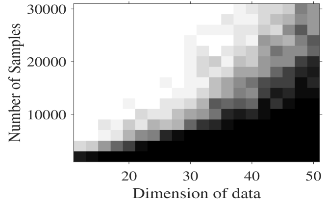
Figure 11: $n$ versus $d$

• The boundary line of black and white parts is almost straight, indicating an approximate linearity between $n$ and $d$.

.45

Figure 12: $\|\widehat{\bfW}-\bfW^{*}\|_{F}$ against $\sqrt{\log n/n}$.

• When $n$ increases, i.e., when $\sqrt{\log n/n}$ decreases, the distance between $\widehat{\bfW}$ and $\bfW^{*}$ decreases.

Empirical experiments

.45

Figure 13: $n$ versus $\boldsymbol{\mu}$

• The sample complexity increases with $\mu$.

.45

Figure 14: $n$ versus $\boldsymbol{\Sigma}$

• The sample complexity first decrease and then increase as $\sigma$ increases.

Empirical experiments

[t] .45

Figure 15: Convergence rate with different $\boldsymbol{\mu}$

• Converges slower as $\mu$ increases.

.45

Figure 16: Convergence rate with different $\boldsymbol{\Sigma}$

• Converges fastest when $\|\Sigma^{\frac{1}{2}\|}$=1.

Conclusion and future work

• We study the problem of learning a fully connected neural network when the input features belong to the Gaussian mixture model from the theoretical perspective.
  

• We propose a gradient descent algorithm with tensor initialization, and the iterates are proved to converge linearly to a critical point with guaranteed generalization.
  

• We characterize the sample complexity for successful recovery, and the sample complexity is proved to be dependent on the parameters of the input distribution.
  

• Future direction: multi-layer neural networks and multi-task learning.

Thank you!

Tensor initialization

1. Estimate the subspace spanned by $\{\bfw_{1}^{*},\cdots,\bfw_{K}^{*}\}$.
   

2. Estimate the direction of $\bfw_{i}^{*},\ i\in[K]$ using the KCL algorithm [Kuleshov et al., 2015].
   

3. Estimate the magnitude of $\bfw_{i},\ i\in[K]$ by solving a linear system.

References

References

• Song Mei, Andrea Montanari, and Phan-Minh Nguyen. A mean field view of the landscape of two-layer neural networks. Proceedings of the National Academy of Sciences, 115(33):E7665-E7671, 2018.

• Lénaïc Chizat and Francis Bach. On the global convergence of gradient descent for overparameterized models using optimal transport. In Proceedings of the 32nd International Conference on Neural Information Processing Systems, NIPS’18, page 3040-3050, 2018.

• Cong Fang, Yihong Gu, Weizhong Zhang, and Tong Zhang. Convex formulation of overparameterized deep neural networks.arXiv:1911.07626, 2019.

• Phan-Minh Nguyen. Mean field limit of the learning dynamics of multilayer neural networks, 2019.

• Arthur Jacot, Franck Gabriel, and Clément Hongler. Neural tangent kernel: Convergence and generalization in neural networks. In Advances in neural information processing systems, pages 8571-8580, 2018.

References

• Zeyuan Allen-Zhu, Yuanzhi Li, and Yingyu Liang. Learning and generalization in overparameterized neural networks, going beyond two layers. In Advances in neural information processing systems, pages 6155-6166, 2019.

• Simon S. Du, Xiyu Zhai, Barnabas Poczos, and Aarti Singh. Gradient descent provably optimizes overparameterized neural networks. In International Conference on Learning Representations, 2019.

• Difan Zou and Quanquan Gu. An improved analysis of training over-parameterized deep neural networks. In H. Wallach, H. Larochelle, A. Beygelzimer, F. dAlché-Buc, E. Fox, and R. Garnett, editors, Advances in Neural Information Processing Systems, volume 32, 2019.

• Difan Zou, Yuan Cao, Dongruo Zhou, and Quanquan Gu. Gradient descent optimizes overparameterized deep relu networks.Machine Learning, 109(3):467-492, 2020.

• Kai Zhong, Zhao Song, Prateek Jain, Peter L Bartlett, and Inderjit S Dhillon. Recovery guarantees for one-hidden-layer neural networks. In Proceedings of the 34th International Conference on Machine Learning-Volume 70, pages 4140-4149, 2017.

References

• Shuai Zhang, Meng Wang, Jinjun Xiong, Sijia Liu, and Pin-Yu Chen. Improved linear convergence of training cnns with generalizability guarantees: A one-hidden-layer case.IEEE Transactions on Neural Networks and Learning System, 2020a.

• Shuai Zhang, Meng Wang, Sijia Liu, Pin-Yu Chen, and Jinjun Xiong. Fast learning of graph neural networks with guaranteed generalizability: One-hidden-layer case.arXiv preprint arXiv:2006.14117, 2020b.

• S. Zhang, M. Wang, S. Liu, P.-Y. Chen, and J. Xiong, “Why lottery ticket wins? a theoretical perspective of sample complexity on sparse neural networks,”Advances in Neural Information Processing Systems,vol. 34, 2021a.

• S. Zhang, M. Wang, S. Liu, P.-Y. Chen, and J. Xiong, “How unlabeled data improve generalization in self-training? a one-hidden-layer theoretical analysis,” in International Conference on Learning Representations, 2021b.

• Haoyu Fu, Yuejie Chi, and Yingbin Liang. Guaranteed recovery of one-hidden-layer neural networks via cross entropy.IEEE Transactions on Signal Processing, 68:3225-3235, 2020.

References

• Yuanzhi Li and Yingyu Liang. Learning overparameterized neural networks via stochastic gradient descent on structured data. In Advances in Neural Information Processing Systems, 2018.

• Yann LeCun, Léon Bottou, Yoshua Bengio, and Patrick Haffner. Gradient-based learning applied to document recognition. Proceedings of the IEEE, 86(11):2278-2324, 1998.

• A. Krizhevsky. Learning multiple layers of features from tiny images. Master’s thesis, Department of Computer Science, University of Toronto, 2009.

• J. Deng, W. Dong, R. Socher, L.-J. Li, K. Li, and L. Fei-Fei. ImageNet: A Large-Scale Hierarchical Image Database. In CVPR09, 2009

• Volodymyr Kuleshov, Arun Chaganty, and Percy Liang. Tensor factorization via matrix factorization. In Artificial Intelligence and Statistics, pages 507–516, 2015.