A Learn-and-Control Strategy for Jet-Based Additive Manufacturing

Abstract

In this paper, we develop a predictive geometry control framework for jet-based additive manufacturing (AM) based on a physics-guided recurrent neural network (RNN) model. Because of its physically interpretable architecture, the model’s parameters are obtained by training the network through back propagation using input-output data from a small number of layers. Moreover, we demonstrate that the model can be dually expressed such that the layer droplet input pattern for (each layer of) the part to be fabricated now becomes the network parameter to be learned by back-propagation. This approach is applied for feedforward predictive control in which the network parameters are learned offline from previous data and the control input pattern for all layers to be printed is synthesized. Sufficient conditions for the predictive controller’s stability are then shown. Furthermore, we design an algorithm for efficiently implementing feedback predictive control in which the network parameters and input patterns (for the receding horizon) are learned online with no added lead time for computation. The feedforward control scheme is shown experimentally to improve the RMS reference tracking error by more than $\boldsymbol{30\%}$ over the state of the art. We also experimentally demonstrate that process uncertainties are compensated by the online learning and feedback control.

I Introduction

Jet-based AM refers to manufacturing techniques in which droplets of a material to be fabricated are deposited onto a substrate based on a input pattern. These droplets then solidify (either by polymerization or solidification), creating a solid layer. As this is carried out layer after layer, the 3D part develops. Like other AM techniques, the additive nature of jet-based AM enables the efficient manufacture of intricate and miniature parts which are otherwise difficult to fabricate. Hence, jet-based AM techniques find application in the manufacture of electronics, medical models, and compliant features for robots and synthetic tissues [1, 2, 3, 4].

A major objective in these applications is to ensure that the droplet deposition results in parts that conform to desired geometry. Several studies have focused on heuristically tuning fabrication parameters such as the rate of deposition, spacing between droplets, and temperature to find the suitable process parameters acceptable [5]. However, these lack a formal relationship between the deposited droplets and the ensuing height profile, which is necessary to optimally control the finished geometry. Moreover, solely heuristic tuning precludes the ability to compensate for droplet or layer height uncertainties during the fabrication process.

The earliest work on 3D part geometry control for jet-based AM was reported in [6] where the authors implemented a so-called greedy geometry feedback scheme on parts made from paraffin wax. A clear drawback of the scheme is its heuristic control law and lack of a droplet deposition model. Subsequent approaches in geometry-level control have incorporated a model into the control scheme. In [7], a stochastic greedy-type control algorithm was employed based on an empirical model. However, this model is not generalizable and suffers from poor scalability. Other researchers have used simplified linear models for control. In [8], the deposited droplets are modelled as a Gaussian distribution and a spatial iterative learning control (SILC) scheme was proposed to minimize geometry tracking error. By design, the SILC is limited to feedforward, or feedback control only if the reference profiles for each layer are identical [9]. In [10] the droplets were assumed to be hemispherical and a predictive feedback controller was proposed and validated in simulation.

Practical implementation of geometry control in high resolution AM requires the process model to be fairly accurate for feedforward control and requires the layer control input patterns to be synthesized in a timely manner for feedback control [11]. [12] experimentally demonstrated model predictive control (MPC) using the linear graph-based model presented in [13]. Though the graph-based model is a substantial simplification of the actual height evolution dynamics, the work showed that by implementing feedback control in a layer-wise fashion, geometries can be accurately tracked, although with increased lead time for computations.

In this work, we use the physics-guided data-driven model presented in [14]. The model is a convolutional RNN (convRNN) with a physically interpretable architecture. This model accurately predicts the height evolution of parts under various scenarios using sparse data. Because of the model’s accuracy, we deploy it for feedforward control and show significantly improved feedforward control performance over the state-of-the-art in [12]. We develop an adaptive control framework in which the model parameters may be updated online while the process is simultaneously controlled in a closed loop fashion. This is made possible due to the low data requirement of the convRNN. The online learning and control frame work follows a strategy presented in [15]. In simulation, the model was learned after each layer and the control input pattern for the next layer was computed. By using the model developed in [14], we allow the learning to occur after an arbitrary number of layers and generalize a nonlinear MPC for an arbitrary number of prediction layers. Moreover, the algorithm is designed efficiently such that no computational lead time, other than that required for measurement, is added to the process and thus may be implemented in practice.

The paper is organized as follows. Table I summarizes relevant notations. In Sec. II we describe the control problem. The following section briefly reviews the state of the art in geometry control in droplet based AM methods. In Sec. IV we develop a predictive controller for the process. The dynamical stability of the predictive controller is analyzed in Sec. V. Sec. VI discusses a strategy for implementing predictive control in an efficient manner. In Sec. VII, we demonstrate both feedforward and feedback (with online learning) control. Sec. VIII concludes the paper and previews future work.

Term	Notation
Reference, measured, model height profile	$R$, $Y$, $\hat{Y}$
Input pattern	$U$
$R$, $Y$, $\hat{Y}$, $U$ vectorized	$r$, $y$, $\hat{y}$, $u$
$U$, $u$ at ${i}^{\textrm{th}}$ layer	$U^{(i)}$, $u^{(i)}$
Set with elements from $i$ to $j$	$\mathcal{U}_{(i)}^{(j)}$
Integers between $0$ and $N$	$[\![0,N]\!]$
Catenation of vectors $u^{(L+i)},i\in[\![0,Z-1]\!]$	$U^{L}$
ConvRNN model parameters	$\theta$
State transition function	$\phi_{1}$
Softplus function	$\phi_{2}$
ConvRNN internal state at time $t$	$h_{t}$
Admissible input matrix at $t$	$U_{t}$
$U_{t}$ vectorized	$u_{t}$
$i^{\textrm{th}}$ element of the vector $u_{t}$	$u_{t}(i)$
Total ConvRNN time steps for layer $L$	$N_{L}$
Initial ConvRNN time step for layer $L$	$t_{0_{L}}$
Convolution kernel	$b$
Toeplitz matrix for $b$ at time $t$	$W_{u,t}$
Sparse Droplet Identifier Matrix	$I_{t}$
$Q$ is a positive semi-definite matrix	$Q\succeq 0$
$P-Q\succeq 0$	$Q\preceq P$
Vector of $n$ 0’s	$\boldsymbol{0}_{n}$
Matrix of $n$ by $n$ 0’s	$\boldsymbol{0}_{n\times n}$
Infinitesimal number	$\delta$
Identity Matrix	$I$
Total number of layers to be printed	$T_{L}$
Prediction/control horizon	$Z$
Layers implemented between measurements	$Z_{u}$
Amount of input-output data pairs used	$\Delta\ell$

TABLE I: Table of relevant notations

II Problem Description

Fig. 1 shows the basic scheme of the jet-based AM system considered in this work, a closed-loop drop-on-demand inkjet 3D printing process. A desired geometry $R$ is to be fabricated. The geometry is resolved in the horizontal plane into an $n_{x}$ by $n_{y}$ grid space to obtained a discretized height distribution (or profile). It is additionally sliced horizontally into layers. Assume we have just printed layer $L$ and the current height profile is $Y^{(L)}\in\mathbb{R}^{n_{x}\times n_{y}}$. Now supposing the desired height profile of the reference geometry at layer $L+Z$ ($Z>0$) is $R^{(L+Z)}\in\mathbb{R}^{n_{x}\times n_{y}}$, we aim to determine the sequence of future input patterns $\mathcal{U}_{(L)}^{(L+Z)}=\{U^{(L)},U^{(L+1)},\ldots,U^{(L+Z-1)}\}$, for $U^{({L+{k}})}\in\mathbb{R}^{n_{x}\times n_{y}},{k}\in[\![0,Z-1]\!]$, that achieve the desired height profile. Moreover, we desire to compensate for process uncertainties or change in the evolution of the height profile. This calls for a feedback control framework in which the system’s model may be adaptively updated in real-time.

To design the control framework, we use the data-driven dynamical model presented in [14] as it lends itself to in-process learning. Consider the function $\Phi$ of [14] parameterized on $\theta$ such that $\hat{Y}^{(L+1)}=\Phi(\theta,{Y}^{(L)},U^{(L)})\in\mathbb{R}^{n_{x}\times n_{y}}$. The optimal set of parameters $\theta^{*}$ is obtained by minimizing the error ${\|{Y}^{(\ell_{f})}-\hat{Y}^{(\ell_{f})}(\theta)\|}_{2}^{2}$ using stored data pairs of $\mathcal{U}_{(\ell_{i})}^{(\ell_{f})}$ and $\{{Y}^{(\ell_{i})},{Y}^{(\ell_{f})}\}$. ${Y}^{(\ell_{i})}$ is the measured initial height profile at layer $\ell_{i}$, upon which the input sequence $\mathcal{U}_{(\ell_{i})}^{(\ell_{f})}$ produces ${Y}^{(\ell_{f})}$ at layer $\ell_{f}$. Once $\theta^{*}$ is obtained, $\Phi$ may be written such that the control input becomes the optimization variable $\hat{Y}^{(L+1)}=\Phi^{*}(\hat{Y}^{(L)},U^{(L)})$. The optimal control input sequence for layers $L$ to $L+Z$, $\mathcal{U}_{(L)}^{(L+Z)*}$, may now be obtained by minimizing ${\|R^{(L+Z)}-\hat{Y}^{(L+Z)}\|}_{2}^{2}$ using the pair ($Y^{(L)}$, $R^{(L+Z)}$). To compensate for uncertainties after printing some layer $L+Z_{u}$ ($Z_{u}\leq Z$), feedback information (the height profile ${Y}^{(L+Z_{u})}$) may be collected and the control input for the next $Z$ layers may be recomputed. To alleviate plant-model mismatch, the set of parameters $\theta$ is updated using data pairs obtained of $\{{Y}^{(\ell_{i})},{Y}^{(\ell_{f})}\}$ and $\mathcal{U}_{(\ell_{i})}^{(\ell_{f})}$ during the printing session. Subsequently, our two-fold objectives are: (1) to develop a procedure for finding optimal control sequence $\mathcal{U}_{(L)}^{(L+Z)*}$; and (2) to generate an efficient strategy for an online update of set $\theta^{*}$ and implementing feedback control.

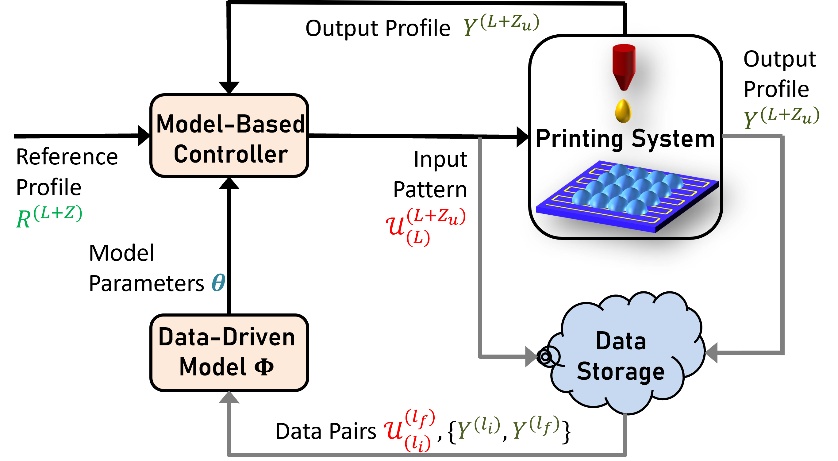
Figure 1: 3D inkjet printing scheme. For each layer, a reference profile based on the desired part geometry is fed to a controller which generates a suitable input sequence.

III Related Work

In Sec. I, we note that several strategies have been employed for geometry-level feedback control in jet-based AM processes. In this section, we summarily discuss these control strategies and assess the drawbacks that springboard the control framework presented in this work.

Greedy Feedback Control: Early attempts to implement geometry-level control involved using greedy algorithms to determine when and where to deposit droplets. In [6], the next location to deposit a droplet was chosen based on a heuristic score assigned to each location. The algorithm is quite limited as it does not consider droplet interaction post-deposition or droplet size/scale. In [7] a ‘stochastic greedy-type’ search algorithm is employed to minimize tracking error $\|R-\hat{Y}^{(L)}\|_{2}^{2}$ and surface roughness. This algorithm empirically models the effect of neighboring droplets when the edges of the part shrink. Consequently, it is not applicable in scenarios where the edges are elevated [14]. Further, due to the ‘greedy’ search approach employed, the algorithm increases in expense proportionally to the size of the grid resolution.

Linear Time-Invariant MPC: In [12], following the lifted model of [16], the geometry control objective is formulated as an MPC problem, where a height-tracking cost-function $J$ is to be minimized over a finite receding horizon of $Z$ layers:

$$\underset{U^{(L)}}{\text{min}} J\left(U^{L}\right)$$ (1)

s.t. $$\hat{y}^{(L+k+1)}=\mathcal{A}\hat{y}^{(L+k)}+\mathcal{B}u^{(L+k)},{k}\in[\![0,Z-1]\!],$$

$$U_{\text{low}}\leq{U^{L}}\leq U_{\text{high}},$$

where $U^{L}=[u^{(L)^{T}}~{}...~{}u^{(L+Z+1)^{T}}]^{T}\in\mathbb{R}^{nZ}$, $u^{(L+k)}$ is the $i^{th}$ layer control input in the receding horizon, and $\hat{y}^{(L)}$ is the current height. $(\mathcal{A},{\mathcal{B}})$ models the height evolution from layer to layer: $\mathcal{A}\in\mathbb{R}^{n\times n}$ is the state matrix that captures the dynamics of the height evolution over the entire layer; ${\mathcal{B}}\in\mathbb{R}^{n\times n}$ is the input matrix accounting for the height distribution of each droplet on deposition. The cost function is designed to penalize tracking error. $U_{\text{low}}$ and $U_{\text{high}}$ define the upper and lower constraints on the input. The optimization is performed each layer, and $u^{(L)^{\star}}$ is applied. The model $({\mathcal{A}},{\mathcal{B}})$ does not adequately capture nonlinear fluid behavior when droplets overlap. Hence, the control approach requires layer-to-layer feedback to adequately compensate for the plant-model mismatch, in addition to compensating for uncertainties. Further, if operating conditions change, the model would require offline re-identification.

Iterative Learning Control: In [8], a spatial iterative learning (SILC) scheme is proposed with the following learning law:

$$u^{(L+1)}=\Gamma_{u}u^{(L)}+\Gamma_{e}e^{(L)}$$ (2)

Here, $\Gamma_{u},\Gamma_{e}\in\mathbb{R}^{n\times n}$ are the input and error learning matrices. $e^{(L)}$ is the error between the desired and model output: $e^{(L)}={y}^{(L)}-\hat{y}^{(L)}$. $\hat{y}^{(L)}$ is evaluated in a similar way as in (1), but with $\mathcal{A}=I$. As with the linear MPC strategy, $\Gamma_{u},\Gamma_{e}$ are evaluated to minimize a height tracking cost function. The SILC is limited to feedforward, or feedback control if the reference profiles for each layer are identical [9, 17]. Though promising, typical demonstrations of the SILC scheme have been limited to simulations.

The above approaches have been shown to achieve improvement in geometry output [18, 12]. However, the model performance is limited as the linear models do not well capture the nonlinear fluid behavior when droplets interact. Furthermore, it is difficult to propagate any plant-model mismatch (disturbance) since the reference geometry for each layer is unique. Hence, it is important to use a model that: (1) more accurately captures the fluid behavior, (2) can be refined online if necessary, and (3) can be used to design a control strategy. Next, we employ the model presented in [14] and design a predictive controller based on the model.

IV Predictive Control of the Printing Process

In the physics-guided convRNN model proposed in [14], the model (network) parameters are time invariant, while the input pattern is fed to the network as a time series. In this section, we re-express the model such that the input is now time-invariant. This re-expression allows us determine the (sub)optimal control input pattern by leveraging the similar gradient expressions as were used for the model identification.

IV-A ConvRNN Model Reformulated for Predictive Control

In [14], for a given layer $L$, the time-step to time-step evolution of the height evolution was modeled as:

$$\begin{split}&h_{t+1}=\phi_{1}(h_{t})+\text{vec}~{}(b*U_{t}),\hskip 14.22636ptt\in[\![0,N_{L}-1]\!],\\ &\hat{y}^{(L+1)}=\phi_{2}(\phi_{1}(h_{N_{L}})),\hskip 14.22636pth_{0}=\hat{y}^{(L)},\end{split}$$ (3)

where $h_{t}\in\mathbb{R}^{n}$, $n=n_{x}\times n_{y}$, is the network’s internal state (or height). The function $\phi_{1}(h_{t})$ is defined as:

$$\phi_{1}(h_{t})=h_{t}-D\sigma(\kappa D^{T}h_{t}),$$ (4)

and denoting $h^{(L)}\coloneqq\phi_{1}(h_{N_{L-1}})$, $\phi_{2}(h^{(L)})$ is defined elementwise as:

$$\phi_{2}(h^{(L)}(i))=\log(\gamma+\exp{h^{(L)}(i)+v_{0}}).$$ (5)

In (4), $D\in\mathbb{R}^{n\times n_{l}}$ is an incidence matrix that transforms the height profile vector into height differences across links where $n_{l}$ is the number of links. These differences are then weighted by a flowability constant $\kappa$ such that $\kappa D^{T}h_{t}$ is the effective flow across links at time $t$ due height to differences across each link, $D^{T}h_{t}$. The activation function $\sigma$ thresholds the effective height difference, $\alpha$, across a link that would cause flow at the time $t$. The soft-thresholding is applied to capture surface tension effect. (The reader is referred to [14] for additional details). Meanwhile, $\phi_{2}$ in (5) is a generic softplus function, parameterized on $\gamma$, that is applied to the element-wise sum of the internal state $h^{(L)}$ and a negative scalar $v_{0}$. The softplus function accounts for the curing effect and ensures the output profile $\hat{y}^{(L)}$ is non-negative.

In (3), $b\in\mathbb{R}^{p\times p}$ is a convolution kernel that represents the effect of a droplet deposition on the height profile. $U_{t}\in\mathbb{R}^{n_{x}\times n_{y}}$, $t\in[0,N_{L}-1]$ are the admissible inputs at time step $t$ such that $\sum_{t=0}^{N_{L}-1}U_{t}=U^{(L)}$. The 2D convolution can be expressed as $\text{vec}(b*U_{t})=W_{u}u_{t}$, where $W_{u}$ is a Toeplitz matrix corresponding to kernel $b$ and $u_{t}\in\mathbb{R}^{n}$ is $U_{t}$ vectorized. Thus, we can now rewrite (3) as:

$$h_{t+1}=\phi_{1}(h_{t})+W_{u,t}u^{(L)},t\in[0,N_{L}-1]$$ (6)

Here, $u^{(L)}$ is the input vector for the entire layer and $W_{u,t}=W_{u}I_{t}$. $I_{t}$ is a sparse matrix holding a one at each position corresponding to where a deposition may take place: $I_{t}u^{(L)}=u_{t}$. Once the model parameters in (3) are identified and given a reference profile, we can find a (sub)optimal input for layer $L$, $u^{(L)*}$ by gradient-based means.

IV-B Predictive Control Using the Reformulated Model

In [14], the optimal values of the model parameters were determined from input-output data. These values were determined via gradient descent direction using back-propagation through time. Now, we follow an analogous approach to determine (sub)optimal input, given knowledge of the model parameters and desired output. Assume layer $L$ has been printed and we are concerned with the output of the next $Z$ layers. We define cost function $J({U^{L}})\mathrel{\ensurestackMath{\stackon[1pt]{=}{\scriptstyle\Delta}}}\sum_{i=0}^{Z}J^{(L+i)}$ where:

$$J^{(L+i)}=\begin{cases}\norm{P(r^{(L+Z)}-\hat{y}^{(L+Z)})}_{2}^{2}&{i=Z},\\ \norm{Q(r^{(L+i)}-\hat{y}^{(L+i)})}_{2}^{2}+\norm{Gu^{(L+i)}}_{2}^{2}&\textrm{else.}\end{cases}$$

The control optimization problem may be written as:

$${U^{L^{*}}} =\underset{{U^{L}}}{\text{argmin }}J({U^{L}})$$ (7a)

$$\text{s.t. }h_{t_{k}+1} =\phi_{1}(h_{t_{k}})+W_{u,t_{k}}u^{(L)},t_{k}\in[\![t_{0_{k}},N_{L+k}-1]\!],$$ (7b)

$$\hat{y}^{(L+k+1)} =\phi_{2}(\phi_{1}(h_{N_{L+k}})),h_{t_{0_{k}}}=\hat{y}^{(L+k)}$$ (7c)

$$\boldsymbol{0}_{n} \leqslant{u^{(L+k)}}\leqslant\boldsymbol{1}_{n}u_{max}~{}\forall k\in[\![0,Z-1]\!]\,$$ (7d)

where $P$, $Q$, $G$ $\in\mathbb{R}^{n\times n}$ are weighting matrices, and $u_{max}$ is an upper bound to the values in ${U^{L*}}$. The total derivative of $J^{(L+i)}$ with respect to $U^{L}$ is:

$$\dfrac{dJ^{(L+i)}}{{dU^{L}}}=\partialderivative{J^{(L+i)}}{\hat{y}^{(L+i)}}\partialderivative{\hat{y}^{(L+i)}}{{U^{L}}}+\partialderivative{J^{(L+i)}}{{U^{L}}}$$

$$=\partialderivative{J^{(i)}}{\hat{y}^{(L+i)}}\sum\limits_{j=0}^{i}\sum\limits_{t_{j}=t_{0_{j}}}^{N_{j}}\partialderivative{\hat{y}^{(L+i)}}{h_{t_{j}}}\partialderivative{h_{t_{j}}}{{U^{L}}}+\partialderivative{J^{(L+i)}}{{U^{L}}}.\quad$$ (8)

The terms in (IV-B) may be expressed as:

$$\partialderivative{J^{(L+i)}}{\hat{y}^{(L+i)}} =\begin{cases}2({r^{(L+Z)}}-\hat{y}^{(L+Z)})^{T}P~{}\textrm{for }i=Z,\\ 2({r^{(L+i)}}-\hat{y}^{(L+i)})^{T}Q~{}\textrm{otherwise },\end{cases}$$ (9)

$$\partialderivative{\hat{y}^{(L+i)}}{h_{t_{j}}} =\partialderivative{\hat{y}^{(L+i)}}{h_{N_{L+i}}}\partialderivative{h_{N_{L+i}}}{\hat{y}^{(L+i-1)}}\cdots\partialderivative{\hat{y}^{(L+j)}}{h_{N_{L+j}}}\partialderivative{h_{N_{L+j}}}{h_{t_{j}}},$$ (10)

$$\partialderivative{h_{t_{j}}}{{U^{L}}} =W_{t_{j}}=\begin{bmatrix}\boldsymbol{0}_{n\times n}^{(0)}\cdots\boldsymbol{0}_{n\times n}^{(i-1)}W_{u,t_{i}}\cdots\boldsymbol{0}_{n\times n}^{(Z-1)}\end{bmatrix},$$ (11)

$$\partialderivative{J^{(L+i)}}{{U^{L}}} =\begin{cases}0&~{}\textrm{for }i=Z,\\ u^{(i)^{T}}G&~{}\textrm{else; }\end{cases}$$ (12)

where:

$$\partialderivative{\hat{y}^{({L+j})}}{h_{N_{L+j}}} =diag(1/(1+\gamma\exp{\boldsymbol{1}v_{0}-{h}_{N_{L+j}}})),$$ (13)

$$\partialderivative{h_{N_{L+j}}}{h_{t_{j}}} =\prod_{N_{L+j}-1>k\geqslant{t_{j}}}\bigg{(}I-Ddiag(\sigma^{\prime}(l_{k}))KD^{T}\bigg{)}.$$ (14)

Then we can write that $\partialderivative{\hat{y}^{(L+i)}}{{U^{L}}}=\partialderivative{\hat{y}^{(L+i)}}{h_{N_{L+i}}}\partialderivative{h_{N_{L+i}}}{{U^{L}}}$ where:

$$\partialderivative{h_{N_{L+i}}}{{U^{L}}}=\begin{cases}0~{}\textrm{for }i=0,\\ \sum\limits_{t_{1}=t_{0_{i_{1}}}}^{N_{L+1}}\partialderivative{h_{N_{L+1}}}{h_{t_{1}}}W_{t_{1}}~{}\textrm{for }i=1,\\ \sum\limits_{t_{i}=t_{0_{i}}}^{N_{L+i}}\partialderivative{h_{N_{L+i}}}{h_{t_{i}}}W_{t_{i}}+\partialderivative{h_{N_{L+i}}}{\hat{y}^{(L+i-1)}}\partialderivative{\hat{y}^{(L+i-1)}}{{U^{L}}}~{}\textrm{else};\end{cases}\hskip 1000.0pt$$ (15)

Note that since the gradients are expressed analytically rather than as finite differences, the computation to find ${U^{L^{*}}}$ is expedited. We use the sequential quadratic programming method in which the Hessian is estimated using the Broyden–Fletcher–Goldfarb–Shanno algorithm and a penalty function is used to enforce the constraint [19, 20]. The approach is implemented using MATLAB’s fmincon function.

V Predictive Control Stability

In this section, we analyze the stability of the MPC problem. For this analysis, we neglect the shrinkage effect in the output equation ($y=h_{N_{L}+1}$). We follow the Lyapunov’s direct method [21], where the cost function of the finite horizon optimization problem is used to establish stability [22, 23, 24].

The height evolution from time step to time step within layer $L$ can be written as:

$${h_{t+1}=\phi_{1}(h_{t})+B_{t}\norm{u_{t}},\hskip 14.22636ptt\in[\![0,N_{L}-1]\!],}$$ (16a)

$${\hat{y}^{(L+1)}=\phi_{1}(h_{N_{L}}),h_{0}=\hat{y}^{(L)},}$$ (16b)

where $B_{t}=(1/\norm{u_{t}})W_{u}u_{t}\in\mathbb{R}^{n}$,

$$\phi_{1}(h_{t})=(I-DK_{\delta}(h_{t})D^{T})h_{t}=A(h_{t})h_{t}$$ (17)

and $K_{\delta}(h_{t})=diag(k_{\delta})\in\mathbb{R}^{n_{l}\times n_{l}}$. Each diagonal element is defined as:

$$k_{\delta}(i)\mathrel{\ensurestackMath{\stackon[1pt]{=}{\scriptstyle\Delta}}}\begin{cases}\kappa\big{(}1-(1-\delta)\alpha/l_{t}(i)\big{)}&\text{if }l_{t}(i)>{\alpha},\\ \delta\kappa&\text{if }{-\alpha}\leqslant{l_{t}(i)}\leqslant{\alpha},\\ \kappa\big{(}1+(1-\delta)\alpha/l_{t}(i)\big{)}&\text{if }l_{t}(i)<{-\alpha},\end{cases}$$ (18)

with $l_{t}=\kappa D^{T}h_{t}\in\mathbb{R}^{n_{l}}$ and $\underline{\kappa}<\kappa<\bar{\kappa}$ ($\underline{\kappa}$ and $\bar{\kappa}$ are lower and upper bounds on the flowability constant). We can lift the time-step height evolution of (3) for each layer to yield a layer-to-layer height evolution model to obtain $\hat{y}^{(L+1)}=\mathcal{A}_{L}\hat{y}^{(L)}+\mathcal{B}_{L}u^{(L)}$ where $\mathcal{A}_{L}\in\mathbb{R}^{n\times{n}}$ is $\prod_{i=N_{L}}^{0}A(h_{i})$, $\mathcal{B}_{L}\in\mathbb{R}^{n\times{N_{L}}}$ is

$$\Big{[}\begin{matrix}(\prod_{i=N_{L}}^{1}A(h_{i}))B_{0}&(\prod_{i=N_{L}}^{2}A(h_{i}))B_{1}&\cdots\end{matrix}$$

$$\begin{matrix}(\prod_{i=N_{L}}^{t+1}A(h_{i}))B_{t}&(\prod_{i=N_{L}}^{t+2}A(h_{i}))B_{t+1}\end{matrix}\cdots A_{N_{L}}B_{N_{L}-1}\Big{]},$$

and we denote $\begin{bmatrix}\norm{u_{0}}&\norm{u_{1}}&\cdots&\norm{u_{t}}&\cdots&\norm{u_{N_{L}-1}}\end{bmatrix}^{T}\equiv u^{(L)}$. Note that $\mathcal{A}_{L}$ and $\mathcal{B}_{L}$ are functions of $\hat{y}^{(L)}$ and $u^{(L)}$, and may be explicitly written as $\mathcal{A}(\hat{y}^{(L)},u^{(L)})$ and $\mathcal{B}(\hat{y}^{(L)},u^{(L)})$ respectively. For brevity, we retain earlier notations.

Let error $e^{(L)}=r^{(L)}-\hat{y}^{(L)}$, where $r^{(L)}$ is the reference height profile for layer $L$. We assume there exists an ideal control input $u^{*(L)}$ such that $r^{(L+1)}=\mathcal{A}_{L}r^{(L)}+\mathcal{B}_{L}u^{*(L)}$. The closed-loop MPC system is now defined as $e^{(L+1)}=\mathcal{A}_{L}e^{(L)}+\mathcal{B}_{L}w^{(L)}$, where $w^{(L)}=u^{*(L)}-u^{(L)}$. The control objective is to minimize the following cost over the next $Z$ layers:

$$\begin{split}&J({W_{L}})\mathrel{\ensurestackMath{\stackon[1pt]{=}{\scriptstyle\Delta}}}(e^{({L+Z})})^{T}Pe^{({L+Z})}\\ &\hskip 10.0pt+\sum_{k=0}^{Z-1}(e^{({L+i})})^{T}Qe^{({L+i})}+(w^{({L+i})})^{T}Gw^{({L+i})}.\end{split}$$ (19)

Stability Lemma: The closed-loop MPC system $e^{(L+1)}=\mathcal{A}_{L}e^{(L)}+\mathcal{B}_{L}f(e^{(L)})$, where $f(e^{(L)})$ is the receding horizon control law that associates the optimal input $w^{*(L)}$ to the current state $e^{(L)}$ is stable at the point $e^{(L)}=0$ if:

1. $P=cP_{D}$ where $c$ is some constant and $P_{D}$ is a diagonal matrix such that $0\preceq P_{D}\preceq I$, and

2. $-P+Q+c\bar{A}^{T}\bar{A}\preceq 0$,

where $Q{\succeq 0}$ and $\bar{A}=(I-\delta{\kappa}DD^{T})$.

Proof: Define the Lyapunov function: $V(e^{(L)})=\underset{W_{L}}{\textrm{min}}J(W_{L})$. Suppose the optimal input sequence is:

$$\begin{split}W_{L}^{\star}(e^{(L)})&=\textrm{arg}\min_{W_{L}}J(W_{L})\\ &=\{w^{*({L})},w^{*({L+1})},\cdots,w^{*({L+Z-1})}\}.\end{split}$$ (20)

The following shifted input sequence at layer $L+1$ is:

$$\begin{split}\tilde{W}_{{L+1}}(e^{({L+1})})=&\{w^{*({L+1})},\cdots,F_{{L+Z}}e^{({L+Z})}\},\end{split}$$ (21)

where $F_{L+Z}$ is some state feedback controller (gain) at $L+Z$. Note $\tilde{W}_{L+1}$ is not necessarily the optimal input at layer $L+1$ for $e^{(L+1)}$. Let $\tilde{V}(e_{L+1})=J(\tilde{W}_{L+1})$. We have:

$${}\begin{split}&\tilde{V}(e^{(L+1)})-V(e^{(L)})=-(e^{(L)})^{T}Qe^{(L)}-(u^{(L)})^{T}Gu^{(L)}\\ &+(e^{(L+Z)})^{T}\Big{(}-P+Q+(F_{L+Z})^{T}G(F_{L+Z})\\ &(\mathcal{A}_{L+Z}+\mathcal{B}_{L+Z}F_{L+Z})^{T}P(\mathcal{A}_{L+Z}+\mathcal{B}_{L+Z}F_{L+Z})\Big{)}e^{(L+Z)},\end{split}$$ (22)

The first two terms on the right-hand-side of (22) are non-positive. For the case where $F_{L+Z}=0$, for any $L+Z$, we want to show that the third term is also non-positive. From Lemma Condition 1, it can be proved that

$$\mathcal{A}_{L+Z}^{T}P\mathcal{A}_{L+Z}\preceq c\bar{A}^{T}\bar{A}~{}\forall~{}{L+Z}.$$ (23)

Since $-P+Q+c\bar{A}^{T}\bar{A}\preceq 0$ (Lemma Condition 2), we have:

$$-P+Q+\mathcal{A}_{L+Z}^{T}P\mathcal{A}_{L+Z}\preceq-P+Q+c\bar{A}^{T}\bar{A}\preceq 0~{}\forall{L+Z}.$$

Thus, $\tilde{V}(e^{(L+1)})-V(e^{(L)})\leq 0~{}\forall~{}e_{L}\neq 0$. Now, noting that $\tilde{W}_{L+1}(e^{L+1})$ (for the case $F_{L+Z}=0$) is not necessarily optimal, it follows that:

$${V}(e^{(L+1)})-V(e^{(L)})\leq\tilde{V}(e^{(L+1)})-V(e^{(L)})\leq 0~{}\forall~{}e_{L}.$$ (24)

Proof of Equation (23): We want to show that $\mathcal{A}_{L}^{T}P\mathcal{A}_{L}\preceq\bar{A}^{T}\bar{A}$ $\forall L$. Let ${A}_{t}=I-DK_{t}D^{T}$, where $K_{t}=K_{\delta}(h_{t})$ as already defined. Recall that $P=cP_{D}$, where $P_{D}\preceq I$ (Lemma Condition 1), and $\bar{A}=(I-\delta{\kappa}DD^{T})$. The inequality may then be written as:

$${A_{N_{L}}}\cdots{A_{0}}P_{D}{A_{0}}\cdots{A_{N_{L}}}\preceq\bar{A}^{T}\bar{A}$$ (25)

Let $\mathcal{S}$ denote the set of all positive definite matrices with spectral radii less or equal to $1$, $\mathcal{S}=\{S:0\preceq S\preceq I;S=S^{T}\}$. To prove (25), we need to show that for any element $M\in\mathcal{S}$, $A_{t}^{T}MA_{t}\in\mathcal{S}$ $\forall~{}t$. [14] establishes that the spectral radius of the Laplacian $DD^{T}$, $\rho(DD^{T})\leqslant 12$. Further, the lower and upper bounds on the flowability constant $\kappa$ ($\underline{\kappa}$ and $\bar{\kappa}$) were given as $0$ and $1/6$ respectively. Since $K_{t}$ is diagonal,

$$2(K_{t}-\delta\underline{\kappa}I)^{-1}\succeq 12I\succeq D^{T}D.$$ (26)

The second inequality follows from $\rho(DD^{T})\leqslant 12$. Hence:

$$2(K_{t}-\delta\underline{\kappa}I)\succeq(K_{t}-\delta\underline{\kappa}I)D^{T}D(K_{t}-\delta\underline{\kappa}I),$$ (27)

which evaluates to:

$$I-2\delta\underline{\kappa}DD^{T} +(\delta\underline{\kappa})^{2}DD^{T}DD^{T}\succeq$$

$$I-2DK_{t}D^{T}+DK_{t}D^{T}DK_{t}D^{T}.$$ (28)

Thus, $\bar{A}^{T}\bar{A}\succeq A_{t}^{T}A_{t}$ for any $t$. By definition, $M\preceq I$, therefore:

$$A_{t}^{T}MA_{t}\preceq A_{t}^{T}A_{t}\preceq\bar{A}^{T}\bar{A}\preceq I~{}~{}\forall t.$$ (29)

Furthermore, for any $M\in\mathcal{S}$, $M\succeq 0$ and so $A_{t}^{T}MA_{t}\succeq 0$; thus (29) can be expanded as:

$$0\preceq A_{t}^{T}MA_{t}\preceq A_{t}^{T}A_{t}\preceq\bar{A}^{T}\bar{A}\preceq I~{}~{}\forall t.$$ (30)

Finally, (30) implies that $A_{t}^{T}MA_{t}\in\mathcal{S}$ $\forall t$. This result indicates that to guarantee stability, $P_{D}$ should be chosen such that $P_{D}\succeq\bar{A}^{T}\bar{A}$, and then, $0\preceq Q\preceq P-c\bar{A}^{T}\bar{A}$.

VI Learn & Control: Feedback Control Strategy

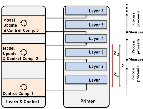
Figure 2: Illustration of feedback MPC strategy to eliminate downtime for online model learning and control computation.

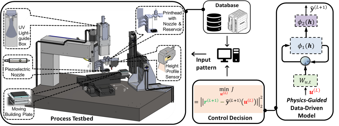
(a)

(b)

Figure 3: (a) Schematic of the control execution. The input pattern for each layer is generated using the convRNN-model-based controller. The computer directs the motion stages and nozzle droplet deposition based on the input pattern. The part is cured under UV light after each layer and the height is measured and stored as data for model training and control. (b) Feedforward control. The model parameters are learned from a printed cross shape; these parameters are now used for MPC of other parts. The parameters of $\theta^{*}$ for the cross shape are given on the right.

Given an accurate model of the height evolution, the optimal control scheme of Section IV-B can provide good tracking performance. As the number of layers increases however, uncertainty in the printing process may begin to substantially impact the height profile evolution. In addition, given that the MPC depends on a data-driven model, we may want to update the model online utilizing data from the current print session (especially if geometry or printing conditions change). The computational expense of updating (training) the model and computing new control input may lead to substantial lead times in the fabrication process. Therefore, in this section, we discuss a strategy for efficient adaptive feedback control. We propose a semi-feedback approach that allows printing and computation to occur simultaneously. This strategy considers that the actual process is relatively slow and that necessary computations will be made in parallel with the printing of one or more layers.

We begin by implementing the MPC similar to the traditional fashion, that is, we calculate input for $Z$ layers in the horizon, implement $Z_{u}$ layer(s) and obtain feedback; but while recomputing control input for the next $Z$ layers, we proceed to print $Z_{d}$ layer(s). The algorithm is demonstrated in Fig. 2 for a 6-layer part and proceeds as follows:

1. Given the total number of layers to be printed $T_{L}$ and control horizon $Z$, set the data size to be used for training as $\Delta\ell$. Also select the number of layers $Z_{u}$ that will be implemented before obtaining the next feedback measurement, such that $Z_{u}+Z_{d}\leq Z$ and $Z_{u}>Z_{d}$. Let $L=0$ and define $T_{s}\mathrel{\ensurestackMath{\stackon[1pt]{=}{\scriptstyle\Delta}}}\left\lfloor(T_{L}-(Z_{d}+Z_{u}))/Z_{u})\right\rfloor$.

2. Use the last $\Delta\ell$ input layer pairs in the data base to identify the set of model parameters. If $\Delta\ell=0$, assume the parameters are based on linear superposition.

3. Calculate the control input for $Z$ layers into the future.

4. For $i={0}\cdots{T_{s}}$:

   1. Implement control input for $Z_{u}$ layers into the future.

   2. Get feedback measurement of the height profile $L=L+Z_{u}$ and add to database.

   3. Proceed to print $Z_{d}$ more layers. Simultaneously, update model parameters using the $\Delta\ell$ last input layer pairs in the augmented data base and calculate the control input for the next $Z$ layers, fixing $\big{[}u^{(L)^{T}}\cdots u^{(L+Z_{d}-1)^{T}}\big{]}^{T}$ already being implemented.

   4. Set $L\leftarrow L+Z_{d}$. If $i=1$, set $~{}Z_{u}\leftarrow Z_{u}-Z_{d}$.

VII Experimental Results

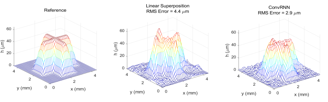
(a) Height profile

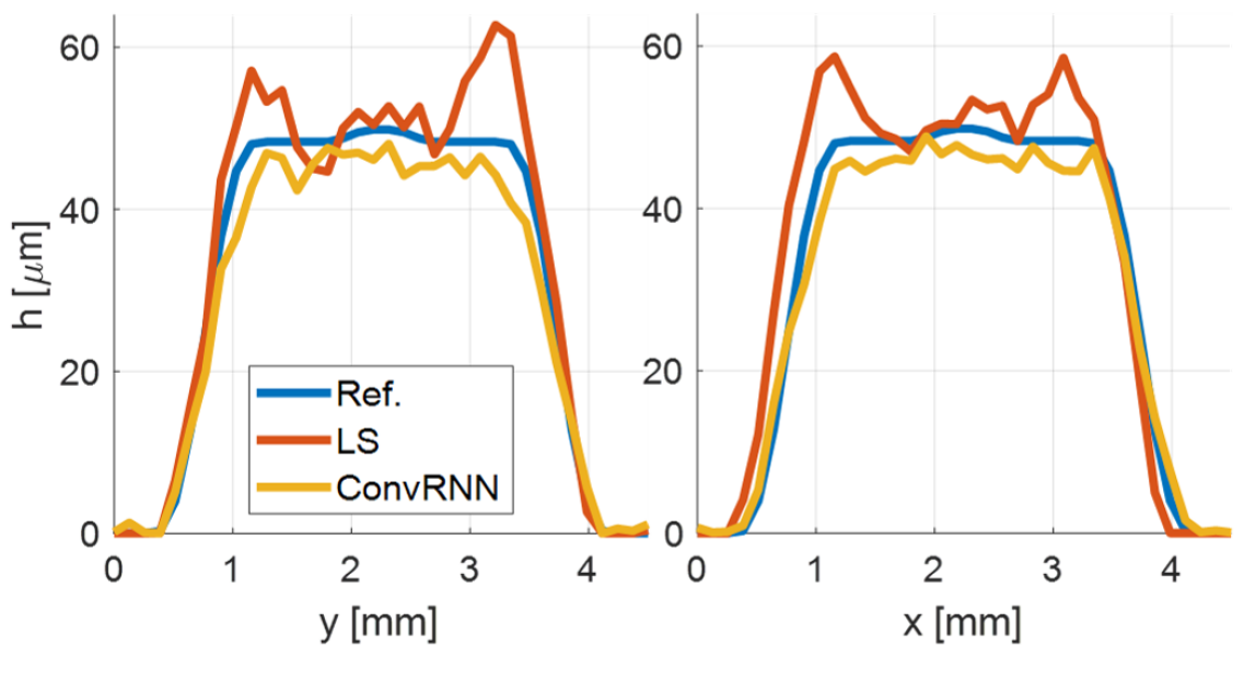
(b) Longitudinal section

Figure 4: Comparison of performance between the linear-superposition-based feedforward control and the convRNN-based feedforward control for a 4-layer cross-shape part. The measured grid resolution is $36\times 36$.

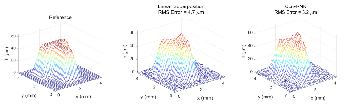
(a) Height profile

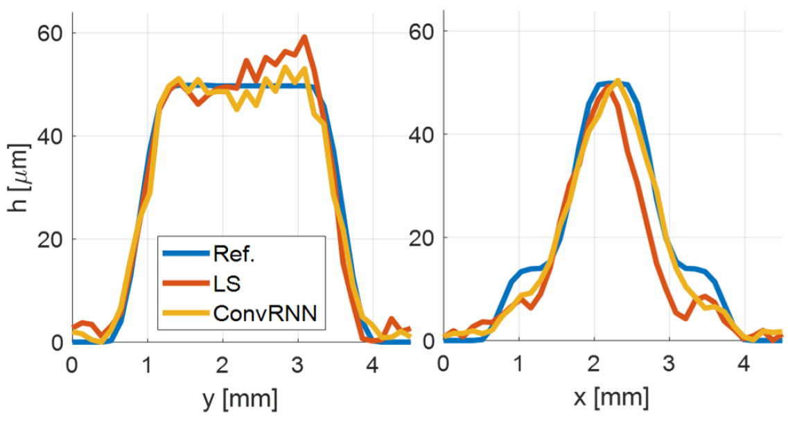
(b) Longitudinal section

Figure 5: Comparison of performance between the linear-superposition-based feedforward control and the convRNN-based feedforward control for a 4-layer T-shape part. The measured grid resolution is $36\times 36$.

Fig. 3(a) shows the experimental setup for control execution. Initially, the 3D model of a part is sliced horizontally into layers and an associated motion path for the nozzle is generated, along with droplet deposition locations. Motion stages move the build substrate while the nozzle deposits droplets according to the input pattern. Once all depositions for a layer are complete, the part is cured under UV light. Then a laser sensor measures the layer height profile for feedback control. The process is repeated until all layers are printed.

Grid size ($n_{x}\times n_{y}$)	$18\times 18$
Grid spacing	281.75$\mu$m
Ink type	Stratsys’ TangoBlack FLX973
Substrate	Cured TangoBlack FLX973
Volatge waveform[25]	Bipolar (60V, 20$\mu$s dwell time)

TABLE II: Printing process parameters

VII-A Feedforward Control Implementation

In this subsection, we experimentally implement the feedforward MPC in Sec. IV-B. The driving signal applied to the piezoelectric nozzle (see [25] for details), the ink type, substrate, and the grid dimensions used for the experiment are given in Table II. We print four layers of a cross shaped part. The convRNN model parameters are learned from this print using the single data pair, $\{{Y}^{(0)},{Y}^{(4)}\}$ and $\mathcal{U}_{(0)}^{(3)}$ (Fig. 3(b)). The identified parameters are given in Fig. 3(b). First, we attempt to find a feedforward control input for a similar cross shape. We find the input pattern for each layer as specified in Sec IV-B, solving for $U^{0}\in\mathbb{R}^{4n}$ with $u_{max}=2$. Because the system is limited to discrete droplets, the solution is quantized by rounding up to the nearest integer and implemented. For comparison, a second cross-shape part with the same reference is printed based on the linear superposition model described in [16]. The cross-shape parts printed based on the linear superposition and the convRNN models are meshed in Fig. 4(a). Note that the sensor measurement gives a finer resolution ($36\times 36$) than the above grid size. The convRNN-based control yields a $34\%$ improvement in RMS tracking error over that of the linear superposition. Longitudinal sections through the parts (Fig. 4(b)) accentuate the convRNN-based control compensation for elevation of the cross edges. We then carry out similar feedforward control for a 4-layered T-shape part (Fig. 5(a)) using only the original identified model parameters $\theta^{*}$ from the cross shape. Similar RMS tracking error performance improvement is observed. Fig. 5(b) shows longitudinal sections through the T-shape part. We observe that the convRNN-based controller not only compensates for elevation of the surface edges, but it also rectifies mismatches in the side walls. An improvement of the reference tracking for all layers (not shown) is also noted.

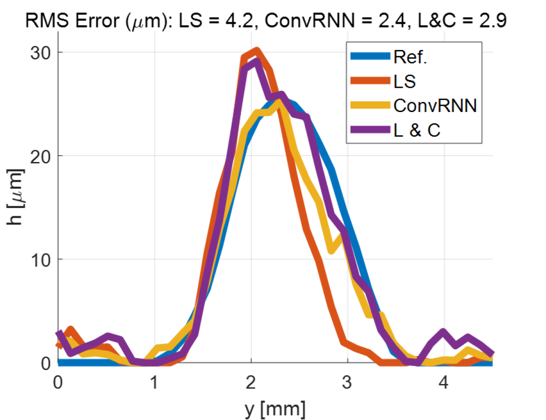
(a) Layer 2

(b) Layer 4

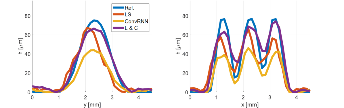
(c) Layer 6

Figure 6: Longitudinal sections of open and closed loop (online learning & control) profiles after every other layer of an N-shaped part. At the top of each subplot is displayed the RMS error of each control approach with respect to the reference.

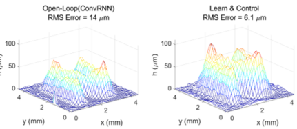
Figure 7: Comparison of feedforward control performance of the convRNN with the learn & control algorithm for an N-shape part. RMS error is based on the reference profile (not shown).

VII-B Online Learning and Control Implementation

We demonstrate the learn & control strategy in Sec. VI using an ‘N’ shape printed in the same fashion as the parts in Sec. VII-A. We first print 6 layers of the part in open-loop based on the linear superposition model. We print 6 additional layers of the part using a feedforward control input that relies on the identified convRNN model $\theta^{*}$ used in Sec. VII-A. Fig. 7 summarizes the results. The figure presents longitudinal sections through the printed part every other layer. Although the convRNN-based feedforward result outperforms that of the superposition at lower layers, as the number of layers grows, bias in the learned $\theta^{*}$ begin to dominate and convRNN-based feedforward is no longer advantageous. Recall that the convRNN feedforward input is based on merely one data pair (the cross-shaped part in Sec. VII-A). Not only does the cross-shape part have fewer layers than the N-shape part, the shrinkage observed in printing this N-shaped part is more significant than for the former. Hence, it is imperative to populate the dataset and learn from it as printing proceeds. Thus, we now print the same ‘N’ shape with learn & control strategy developed in Sec. VI as illustrated in Fig. 2. The following parameters are used: $Z=3,~{}Z_{u}=2,~{}Z_{d}=1$.

Results for the online learning and feedback control strategy are superimposed on Fig. 6 (purple line). Observe that the feedforward output based on the linear superposition model exhibits the largest RMS error at the 2nd layer (Fig. 6(a)). This is because this model only accounts for droplet deposition and does not capture any further dynamics. The feedforward convRNN, with a control horizon of $Z=6$, has the best performance at this layer. (Note that the learn & control strategy is solving a different MPC problem with $Z=3$). The learn & control algorithm takes the lowest RMS error at the 4th layer (Fig. 6(b)) because of feedback. Although the feedforward convRNN profile is better laterally aligned with the reference than the linear superposition model, the volume of material being deposited is inadequate. By the final layer (Fig. 6(c)), this volume inadequacy results in the greatest deviation from the reference. On the other hand, the learn & control feedback algorithm improves the RMS error over the convRNN-based feedforward profile by over $50\%$ (Fig. 7) and the superposition-based feedforward profile by $45\%$. Using a 4.1 GHz Intel Core i7 16GB RAM computer, the computational time required for online model update and control calculations is about a half minute or less. Meanwhile, the typical print time for a layer is about 4 minutes. Since the computations and printing occur simultaneously, no additional lead time is required.

Discussion: We have demonstrated that we can achieve significant improvement in reference geometry tracking in the inkjet 3D printing process using a feedback control scheme with minimal downtime. The height profile need not be measured frequently and the computations required for model training and control learning, though expensive, may be carried out simultaneously with the printing process. These benefits are made possible through a physics-guided data-driven model that requires little data for training and is a good predictor of the process dynamics. For larger grid sizes, the computational time will grow exponentially while the actual printing time grows linearly [12]. Hence, future work will address decentralization of the MPC scheme to scale it almost linearly with grid size.

VIII Conclusions

In this paper we proposed a novel predictive control method to improve geometry accuracy in jet-based AM. Our method improves upon existing linear MPC and iterative learning control methods by using a physics-guided data-driven model that captures the nonlinear fluid behavior of interacting droplets. We showed how the nonlinear predictive controller may be synthesized using backpropagation gradients. We also established conditions for stability of the controlled system. We implemented the feedforward nonlinear MPC scheme and showed it to outperform the state-of-the-art open-loop control for inkjet 3D printing. We further developed an efficient online learning and control algorithm that allows for feedback control in real time without adding substantial lead time to the fabrication process. The algorithm was also implemented on an inkjet 3D printing system and shown to substantially improve the reference geometry tracking over open-loop printing. Future work will aim to distribute the MPC optimization for faster computation and implement the feedback control strategy in multi-material printing.

References

- [1] S. F. S. Shirazi et al., “A review on powder-based additive manufacturing for tissue engineering: Selective laser sintering and inkjet 3D printing,” Sci. Technol. Adv. Mater., vol. 16, no. 3, 2015.
- [2] M. Singh, H. M. Haverinen, P. Dhagat, and G. E. Jabbour, “Inkjet printing - process and its applications,” Advanced Materials, vol. 22, no. 6, pp. 673–685, 2010.
- [3] Y. Guo, H. S. Patanwala, B. Bognet, and A. W. Ma, “Inkjet and inkjet-based 3D printing: Connecting fluid properties and printing performance,” Rapid Prototyping J., vol. 23, no. 3, pp. 562–576, 2017.
- [4] T. Wang, T. H. Kwok, and C. Zhou, “In-situ Droplet Inspection and Control System for Liquid Metal Jet 3D Printing Process,” Procedia Manufacturing, vol. 10, no. 514, pp. 968–981, 2017.
- [5] X. Qi, G. Chen, Y. Li, X. Cheng, and C. Li, “Applying neural-network-based machine learning to additive manufacturing: Current applications, challenges, and future perspectives,” Engineering, vol. 5, no. 4, pp. 721 – 729, 2019.
- [6] D. L. Cohen and H. Lipson, “Geometric feedback control of discrete-deposition sff systems,” Rapid Prototyping Journal, vol. 16, no. 5, pp. 377–393, 2010.
- [7] L. Lu, J. Zheng, and S. Mishra, “A layer-to-layer model and feedback control of ink-jet 3-d printing,” IEEE/ASME Trans. Mechatronics, vol. 20, no. 3, 2015.
- [8] D. J. Hoelzle and K. L. Barton, “On spatial iterative learning control via 2-d convolution: Stability analysis and computational efficiency,” IEEE Trans. Control Syst. Technol., vol. 24, no. 4, pp. 1504–1512, July 2016.
- [9] L. Aarnoudse, C. Pannier, Z. Afkhami, T. Oomen, and K. Barton, “Multi-layer spatial iterative learning control for micro-additive manufacturing,” 8th IFAC Symp. Mechatronic Sys., vol. 52, no. 15, pp. 97–102, 2019.
- [10] Y. Guo and S. Mishra, “A predictive control algorithm for layer-to-layer ink-jet 3d printing,” Amer. Control Conf. (ACC), pp. 833–838, 2016.
- [11] R. G. Landers, K. Barton, S. Devasia, T. R. Kurfess, P. R. Pagilla, and M. Tomizuka, “A review of manufacturing process control,” J. Manuf. Sci. Engineering-Trans. ASME, vol. 142, 2020.
- [12] U. Inyang-Udoh and S. Mishra, “A learning-based approach to modeling and control of inkjet 3d printing,” in Amer. Control Conf. (ACC), 2020, pp. 460–466.
- [13] Y. Guo, J. Peters, T. Oomen, and S. Mishra, “Control-oriented models for ink-jet 3d printing,” Mechatronics, vol. 56, 05 2018.
- [14] U. Inyang-Udoh and S. Mishra, “A physics-guided neural network dynamical model for droplet-based additive manufacturing,” IEEE Trans. Control Syst. Technol., pp. 1–13, 2021.
- [15] U. Inyang-Udoh, Y. Guo, J. Peters, T. Oomen, and S. Mishra, “Layer-to-layer predictive control of inkjet 3-d printing,” IEEE/ASME Trans. Mechatronics, vol. 25, no. 4, pp. 1783–1793, 2020.
- [16] Y. Guo, J. Peters, T. Oomen, and S. Mishra, “Distributed model predictive control for ink-jet 3d printing,” in IEEE Conf. Adv. Intell. Mechatronics (AIM), 2017, pp. 436–441.
- [17] Z. Afkhami, C. Pannier, L. Aarnoudse, D. Hoelzle, and K. Barton, “Spatial Iterative Learning Control for Multi-material Three-Dimensional Structures,” ASME Lett. Dynamic Syst. Control, vol. 1, no. 1, 03 2020.
- [18] Z. Wang, C. P. Pannier, K. Barton, and D. J. Hoelzle, “Application of robust monotonically convergent spatial iterative learning control to microscale additive manufacturing,” Mechatronics, 2018.
- [19] R. Fletcher, Nonlinear Programming. Hoboken, NJ, USA: Wiley, 2000, ch. 12, pp. 277–330.
- [20] M. S. Bazaraa, Nonlinear Programming: Theory and Algorithms, 3rd ed. Wiley Publishing, 2013.
- [21] C. Chen and L. Shaw, “On receding horizon feedback control,” Automatica, vol. 18, no. 3, pp. 349–352, 1982.
- [22] S. S. Keerthi and E. G. Gilbert, “Optimal infinite-horizon feedback laws for a general class of constrained discrete-time systems: Stability and moving-horizon approximations,” J. Optim. Theory Appl., vol. 57, no. 2, pp. 265–293, May 1988.
- [23] J. B. Rawlings and K. R. Muske, “The stability of constrained receding horizon control,” IEEE transactions on automatic control, vol. 38, no. 10, pp. 1512–1516, 1993.
- [24] F. Borrelli, A. Bemporad, and M. Morari, Predictive Control for Linear and Hybrid Systems. Cambridge, UK: Cambridge University Press, 2017.
- [25] MicroFab Tech. Inc., Plano, TX, USA. Ink-Jet Microdispensing Basic Set-up. (2012). Accessed: Nov. 29, 2021.