Three-loop helicity amplitudes for quark-gluon scattering in QCD

Abstract

We compute the three-loop helicity amplitudes for $q\bar{q}\to gg$ and its crossed partonic channels, in massless QCD. Our analytical results provide a non-trivial check of the color quadrupole contribution to the infrared poles for external states in different color representations. At high energies, the $qg\to qg$ amplitude shows the predicted factorized form from Regge theory and confirms previous results for the gluon Regge trajectory extracted from $qq^{\prime}\to qq^{\prime}$ and $gg\to gg$ scattering.

I Introduction

The computation of multiloop scattering amplitudes in Quantum Chromodynamics (QCD) plays a fundamental role for the Standard Model (SM) precision program carried out at particle colliders such as the Large Hadron Collider (LHC) at CERN. Suitably combined with real-radiation contributions, they provide a powerful tool to generate predictions for a variety of collider observables, allowing for precise comparisons with experimental data Heinrich:2020ybq . In fact, matching the shrinking experimental errors with correspondingly precise theory predictions allows one to discover even subtle signals from possible physics scenarios beyond the SM.

In addition to their phenomenological significance, analytic computations of scattering amplitudes enable investigations of general properties of perturbative Quantum Field Theories (QFT), including comparative studies of QCD amplitudes with their supersymmetric counterparts. The more loops, external legs, or particle masses one is considering for a scattering amplitude, the more challenging its computation becomes. In recent years, significant progress has been achieved for the reduction of loop integrals to master integrals and their analytical evaluation, resulting in the calculation of previously inaccessible multiloop amplitudes. At two loops, various QCD amplitudes became available for 2 $\rightarrow$ 3 scattering processes involving mostly massless particles Badger:2017jhb ; Abreu:2017hqn ; Abreu:2018aqd ; Abreu:2018zmy ; Abreu:2018jgq ; Abreu:2019rpt ; Abreu:2020cwb ; Chicherin:2018yne ; Chicherin:2019xeg ; Chawdhry:2020for ; DeLaurentis:2020qle ; Chawdhry:2018awn ; Abreu:2020xvt ; Agarwal:2021grm ; Badger:2021nhg ; Abreu:2021fuk ; Agarwal:2021vdh ; Chawdhry:2021mkw ; Badger:2021imn ; Gehrmann:2015bfy ; Papadopoulos:2015jft ; Gehrmann:2018yef ; Chicherin:2018mue ; Chicherin:2020oor ; Abreu:2021asb ; Badger:2022ncb , paving the way for the first Next-to-Next-to-Leading-Order (NNLO) studies at LHC Chawdhry:2019bji ; Czakon:2021mjy ; Chawdhry:2021hkp . At three loops, first QCD amplitudes were computed for 2 $\rightarrow$ 2 scattering processes Caola:2020dfu ; Caola:2021rqz ; Caola:2021izf ; Bargiela:2021wuy . At four loops, $2\to 1$ form factors were obtained in full-color QCD Lee:2021uqq ; Lee:2022nhh ; Chakraborty:2022yan .

Analytical results for multiloop scattering amplitudes can also provide non-trivial information about all-order results in QCD. An interesting case is the so-called Regge limit Kuraev:1977fs of large collision energy, where universal factorization properties can be observed in QCD amplitudes. The BFKL formalism Kuraev:1976ge ; Balitsky:1978ic allows one to describe all-order structures in QCD through the exchange of so-called “Reggeized gluons”, which resum leading contributions of the quark and gluon interactions at high energies. With the recent determination of the three-loop Regge trajectory Caola:2021izf ; Falcioni:2021dgr , the last missing ingredient for next-to-next-to-leading-logarithmic analysis became available.

This paper concludes our analytical calculation of all four-parton scattering amplitudes in three-loop QCD. Previously, we presented the helicity amplitudes for the process $q\bar{q}\to q^{\prime}\bar{q}^{\prime}$ and crossed channels Caola:2021rqz and for the process $gg\to gg$ Caola:2021izf . In this work, we provide the helicity amplitudes for $q\bar{q}\to gg$ scattering and crossed channels in full-color, massless QCD. Our calculation checks the predicted quadrupole contribution to the infrared poles for a process with external legs in different color representation Almelid:2015jia ; Henn:2016jdu . By analyzing the high-energy limit of the $qg\to qg$ amplitude, we check the universality of the predicted factorization and the three-loop expression for the Regge trajectory Caola:2021izf ; Falcioni:2021dgr .

The rest of this paper is organized as follows. In section II, we set up our notation and describe the color and Lorentz decomposition of the scattering amplitude. In section III we discuss our computation of the bare helicity amplitudes employing the tensor decomposition provided in the previous section and analytical solutions for the master integrals Henn:2020lye ; Bargiela:2021wuy . In section IV, we describe the UV renormalization and give details for the subtraction of IR poles up to three loops. In section V we present our final results and enumerate the checks we have performed to verify their correctness. Finally, in section VI we discuss the high energy (Regge) limit of the $qg\to qg$ amplitudes. We draw our conclusions in section VII. We reserve the appendices for lengthy formulas with explicit results for all the relevant anomalous dimensions (appendix A) and for the impact factors and the gluon Regge trajectory (appendix B).

II Color and Lorentz decomposition

We consider the quark-gluon scattering process

$${q}(p_{1})\;+\;\bar{q}(p_{2})\;+\;{g}(p_{3})\;+\;{g}(p_{4})\;\longrightarrow\;0,$$ (1)

in massless QCD, where the momenta satisfy

$$p_{1}^{2}=p_{2}^{2}=p_{3}^{2}=p_{4}^{2}=0,\qquad p_{1}^{\mu}+p_{2}^{\mu}+p_{3}^{\mu}+p_{4}^{\mu}=0.$$ (2)

The kinematics of the process eq. (1) can be parametrized in terms of the usual Mandelstam invariants

$$s=(p_{1}+p_{2})^{2},\qquad t=(p_{1}+p_{3})^{2},\qquad u=(p_{2}+p_{3})^{2},$$ (3)

with $u=-t-s$. We find it convenient to introduce the dimensionless variable

$$x=-t/s$$ (4)

to parametrize our results.

The primary physical scattering process considered in this paper is

$${q}(p_{1})\;+\;\bar{q}(p_{2})\;\longrightarrow\;{g}(p_{3})\;+\;{g}(p_{4})\,,$$ (5)

which can be obtained from the process (1) by a crossing of external legs with $p_{3,4}\rightarrow-p_{3,4}$. For this process, the physical region of the phase space is given by

$$s>0,\quad t,u<0\qquad\Rightarrow\quad 0<x<1\,.$$ (6)

Results for other physical scattering processes will subsequently be derived from the result for process (5) by considering further crossings. The bare amplitude for process (5) can be decomposed in three different color structures $\mathcal{C}_{i}$,

$$\mathcal{A}_{i_{1},i_{2},a_{3},a_{4}}=4\pi\alpha_{s,b}\sum_{i=1}^{3}\mathcal{A}^{[i]}{\mathcal{C}}_{i}\,.$$ (7)

Here, $i_{1}$ and $i_{2}$ are the fundamental color indices of the external quarks with momenta $p_{1}$ and $p_{2}$, and $a_{3}$ and $a_{4}$ are the adjoint color indices of the external gluons with momenta $p_{3}$ and $p_{4}$, respectively. Further, $\alpha_{s,b}$ is the bare strong coupling. In eq. (7) we also introduced the notation $[i]$ to indicate a color component index of the amplitude. The three color structures are

$${\mathcal{C}}_{1}=({{T}^{a_{3}}}{{T}^{a_{4}}})_{i_{2}i_{1}},\quad\quad{\mathcal{C}}_{2}=({{T}^{a_{4}}}{{T}^{a_{3}}})_{i_{2}i_{1}},\quad\quad{\mathcal{C}}_{3}=\delta^{a_{3}a_{4}}\,\delta_{i_{2}i_{1}}\,,$$ (8)

where we work in QCD with color group $SU(N_{c})$ and $n_{f}$ massless quark flavors. The matrices $(T^{a})_{i_{2}i_{1}}$ are the generators of $SU(N_{c})$ in the fundamental representation. We use $\operatorname{Tr}[T^{a}T^{b}]=\frac{1}{2}\delta_{ab}$ and denote the quadratic Casimir operators in the fundamental and adjoint representation by $C_{F}$ and $C_{A}$, respectively.

The amplitude coefficients $\mathcal{A}^{[i]}$ can be decomposed further into Lorentz-covariant structures $\mathcal{T}_{i}$,

$$\mathcal{A}^{[i]}=\sum_{j=1}^{4}\mathcal{F}^{[i]}_{j}\;\mathcal{T}_{i}\;,$$ (9)

where the $\mathcal{F}^{[i]}_{j}$ are scalar form factors. To regulate ultraviolet and infrared divergences, we employ dimensional regularization and use $d=4-2\epsilon$ for the number of space-time dimensions. We denote the external gluon polarization vectors as $\epsilon(p_{i})=\epsilon_{i}$ with the transversality condition for the external gluon momenta $\epsilon(p_{i})\cdot p_{i}=0$ ($i=3,4$). To simplify the Lorentz decomposition, we also fix the gauge of the external gluons such that $\epsilon_{3}\cdot p_{2}=\epsilon_{4}\cdot p_{1}=0$, which leads to the following gluon polarization sums

$$\sum_{pol}{\epsilon}^{\mu}_{3}{\epsilon}^{\nu}_{3}=-g^{\mu\nu}+\frac{{p}^{\mu}_{3}{p}^{\nu}_{2}+{p}^{\nu}_{3}{p}^{\mu}_{2}}{p_{2}\cdot p_{3}},\,$$

$$\sum_{pol}{\epsilon}^{\mu}_{4}{\epsilon}^{\nu}_{4}=-g^{\mu\nu}+\frac{{p}^{\mu}_{4}{p}^{\nu}_{1}+{p}^{\nu}_{4}{p}^{\mu}_{1}}{p_{1}\cdot p_{4}}\,.$$ (10)

Since we are ultimately interested in computing the helicity amplitudes for this process in the ’t Hooft–Veltman scheme (tHV) scheme, we use the Lorentz structures Peraro:2019cjj ; Peraro:2020sfm ; Caola:2020dfu

$$\mathcal{T}_{1} =\bar{u}(p_{2}){\cancel{\epsilon}}_{3}u(p_{1})\,\epsilon_{4}\cdot p_{2}\,,\quad\quad \mathcal{T}_{2}=\bar{u}(p_{2}){\cancel{\epsilon}}_{4}u(p_{1})\,\epsilon_{3}\cdot p_{1}\,,$$

$$\mathcal{T}_{3} =\bar{u}(p_{2}){\cancel{p}}_{3}u(p_{1})\,\epsilon_{3}\cdot p_{1}\,\epsilon_{4}\cdot p_{2}\,,\quad\quad \mathcal{T}_{4}=\bar{u}(p_{2}){\cancel{p}}_{3}u(p_{1})\,\epsilon_{3}\cdot\epsilon_{4}\,,$$ (11)

and introduce projection operators $\mathcal{P}_{i}$ which extract the form factors from the amplitude,

$$\mathcal{P}_{j}\cdot\mathcal{A}^{[i]}=\sum_{\text{pol}}\mathcal{P}_{j}\mathcal{A}^{[i]}=\mathcal{F}^{[i]}_{j},\quad j=1,\ldots,4\,.$$ (12)

In eq. (12), we introduced the short-hand notation $\mathcal{P}_{i}\cdot\mathcal{A}$ which implies a sum over the polarizations of the external particles. By introducing the matrix

$$M_{ij}=\mathcal{T}^{\dagger}_{i}\cdot\mathcal{T}_{j},$$

the projectors can be compactly defined as

$$\mathcal{P}_{i}=\sum_{j=1}^{4}(M^{-1})_{ij}\mathcal{T}^{+}_{j}\quad\implies\quad\mathcal{P}_{i}\cdot\mathcal{T}_{j}=\delta_{ij}\,,$$ (13)

where

$$M^{-1} =\frac{1}{2(d-3)s^{2}t^{3}u}\left(\begin{array}[]{cccc}t^{2}u^{2}&0&-tu^{2}&0\\ 0&t^{2}u^{2}&tu^{2}&0\\ -tu^{2}&tu^{2}&\,\,(du^{2}-4st)&(s-t)st\\ 0&0&(s-t)st&s^{2}t^{2}\\ \end{array}\right)\,.$$ (18)

We stress that in conventional dimensional regularization there is a fifth Lorentz structure which would need to be taken into account in eq. (9). In the tHV scheme we take internal momenta in $d=4-2\epsilon$ dimensions and keep external momenta and polarizations in four dimensions. As explained in refs. Peraro:2019cjj ; Peraro:2020sfm , this allows us to essentially ignore this fifth evanescent structure completely and work with just the four structures (II), which are linearly independent in four space-time dimensions. We also point out that the decompositions of eqs. (7) and (9), as well as the explicit form of the projectors (13), hold to any orders in perturbation theory.

III Helicity amplitudes

From the form factors $\mathcal{F}_{j}$ one can construct amplitudes for definite helicities of the external particles. We denote the helicity of the incoming quark as $\lambda_{q}$; the helicity of the incoming anti-quark $\lambda_{\bar{q}}$ is then automatically fixed due to helicity conservation along the massless quark line. We refer to the quark line helicity with the symbol $\lambda_{q\bar{q}}=\{\lambda_{q}\lambda_{\bar{q}}\}$ which can take two possible values: $\lambda_{q\bar{q}}=L,R=\{-+\},\{+-\}$. Further, we denote the helicities of the outgoing gluons as $\lambda_{3}$ and $\lambda_{4}$. After exploiting parity, charge-conjugation and Bose symmetry relations Caola:2020dfu , one is left with only two independent helicity configurations. However, we choose to compute the overcomplete set of four helicity configurations

$$\{\lambda_{q\bar{q}}\lambda_{3}\lambda_{4}\}=\{L--\},\{L-+\},\{L+-\},\{L++\}$$ (19)

which allow us to perform a consistency check on our calculation. Results for right-handed quarks can subsequently be obtained by a parity transformation. We write for the left-handed spinors $\overline{u_{L}}(p_{2})=\langle 2|$, $u_{L}(p_{1})=|1]$, and for the polarization vector of the gluons

$$\epsilon^{\mu}_{3,-}(p_{3}) =\frac{\langle 2|\gamma^{\mu}|3]}{\sqrt{2}\langle 23\rangle}\,, \epsilon^{\mu}_{3,+}(p_{3}) =\frac{\langle 3|\gamma^{\mu}|2]}{\sqrt{2}[32]}\,,$$ (20)

$$\epsilon^{\mu}_{4,-}(p_{4}) =\frac{\langle 1|\gamma^{\mu}|4]}{\sqrt{2}\langle 14\rangle}\,, \epsilon^{\mu}_{4,+}(p_{4}) =\frac{\langle 4|\gamma^{\mu}|1]}{\sqrt{2}[41]}\,.$$ (21)

Inserting these equations into the Lorentz structures $\mathcal{T}_{j}$ (II) gives the helicity amplitudes

$$\mathcal{A}_{L--} =s_{L--}\sum_{i=1}^{3}\mathcal{H}^{[i]}_{1}\;{\mathcal{C}}_{i}\,,\quad \mathcal{A}_{L-+} =s_{L-+}\sum_{i=1}^{3}\mathcal{H}^{[i]}_{2}\;{\mathcal{C}}_{i}\,,$$

$$\mathcal{A}_{L+-} =s_{L+-}\sum_{i=1}^{3}\mathcal{H}^{[i]}_{3}\;{\mathcal{C}}_{i}\,,\quad \mathcal{A}_{L++} =s_{L++}\sum_{i=1}^{3}\mathcal{H}^{[i]}_{4}\;{\mathcal{C}}_{i}\,,$$ (22)

where the little group scaling is captured by the overall spinor factors

$$s_{L--}=\frac{2[34]^{2}}{\langle 13\rangle[23]}\,,\quad s_{L-+}=\frac{2\langle 24\rangle[13]}{\langle 23\rangle[24]}\,,\quad s_{L+-}=\frac{2\langle 23\rangle[41]}{\langle 24\rangle[32]}\,,\quad s_{L++}=\frac{2{\langle 34\rangle}^{2}}{\langle 31\rangle[23]}\,,$$ (23)

and we have defined the scalar helicity amplitudes

$$\mathcal{H}^{[i]}_{1} =\frac{t}{2}\left(\mathcal{F}^{[i]}_{2}-\frac{t}{2}\mathcal{F}^{[i]}_{3}+\mathcal{F}^{[i]}_{4}\right), \mathcal{H}^{[i]}_{2} =\frac{t}{2}\left(\frac{s}{2}\mathcal{F}^{[i]}_{3}+\mathcal{F}^{[i]}_{4}\right),$$

$$\mathcal{H}^{[i]}_{3} =\frac{st}{2u}\left(\mathcal{F}^{[i]}_{2}-\mathcal{F}^{[i]}_{1}-\frac{t}{2}\mathcal{F}^{[i]}_{3}-\frac{t}{s}\mathcal{F}^{[i]}_{4}\right), \mathcal{H}^{[i]}_{4} =\frac{t}{2}\left(\mathcal{F}^{[i]}_{1}+\frac{t}{2}\mathcal{F}^{[i]}_{3}-\mathcal{F}^{[i]}_{4}\right).$$ (24)

The amplitudes for right-handed quarks are related to those for left-handed quarks by

$$\mathcal{A}_{R,\lambda_{3},\lambda_{4}}=(\mathcal{A}_{L,-\lambda_{3},-\lambda_{4}})|_{\langle ij\rangle\leftrightarrow[ji]}\,.$$ (25)

By exchanging the two outgoing gluons, we find that Bose symmetry implies the relations

$$\mathcal{H}_{2}^{[1]}(x) = +\mathcal{H}_{3}^{[2]}(1-x),\qquad \mathcal{H}_{2}^{[2]}(x) = +\mathcal{H}_{3}^{[1]}(1-x),\qquad \mathcal{H}_{2}^{[3]}(x) = +\mathcal{H}_{3}^{[3]}(1-x),$$

$$\mathcal{H}_{1,4}^{[1]}(x) = -\mathcal{H}_{1,4}^{[2]}(1-x),\qquad \mathcal{H}_{1,4}^{[2]}(x) = -\mathcal{H}_{1,4}^{[1]}(1-x),\qquad \mathcal{H}_{1,4}^{[3]}(x) = -\mathcal{H}_{1,4}^{[3]}(1-x).$$ (26)

We also note that

$$\mathcal{H}_{1}^{[i]}(x)=-\mathcal{H}_{4}^{[i]}(x)\,.$$ (27)

These identities will serve as an important check of our calculations.

We expand the helicity amplitudes in $\bar{\alpha}_{s,b}\equiv{\alpha_{s,b}}/({4\pi})$,

$$\mathcal{H}^{[i]}_{\lambda} =\sum_{\ell=0}^{3}\mathcal{H}^{[i],(\ell)}_{\lambda}\left(\bar{\alpha}_{s,b}S_{\epsilon}\right)^{\ell}+\operatorname{\mathcal{O}}\left(\bar{\alpha}_{s,b}^{4}\right)$$ (28)

for $\lambda=1,\ldots,4$, where $S_{\epsilon}=(4\pi)^{\epsilon}e^{-\epsilon\gamma_{E}}$. The normalization factor $S_{\epsilon}$ absorbs constants in the bare amplitude and matches the usual $\overline{\text{MS}}$ conventions in the renormalization of the strong coupling performed below. In the expansion of the amplitude, $\mathcal{H}^{[i],(3)}_{\lambda}$ is the three loop contribution, which we compute here for the first time. We have also recomputed the tree-level, one-loop and two-loop contributions using the form factor decomposition defined in eq. (II).

We employ Qgraf Nogueira:1991ex to produce Feynman diagrams and find 3 diagrams at tree level, 30 diagrams at one loop, 595 diagrams at two loops and 14971 at three loops. We give a few representative samples of the three-loop diagrams contributing to the process in figure 1.

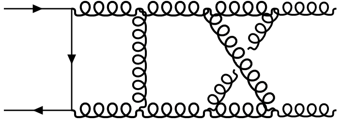
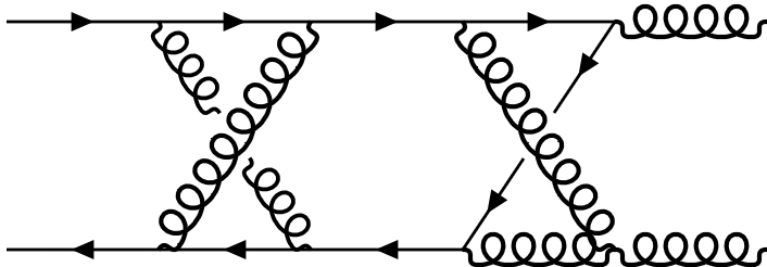
Figure 1: Sample three loop diagrams contributing to the process $q\bar{q}\rightarrow gg$.

We use Form Vermaseren:2000nd to apply the Lorentz projectors of eq. (II) to the diagrams and to perform the Dirac and color algebra. In this way, we obtain the form factors as linear combinations of a large number $(\sim 10^{7})$ of scalar Feynman integrals with rational coefficients. We parametrize the corresponding $\ell$-loop Feynman integrals according to

$$\mathcal{I}^{\text{top}}_{n_{1},n_{2},...,n_{N}}=\mu_{0}^{2\ell\epsilon}e^{\ell\epsilon\gamma_{E}}\int\prod_{j=1}^{\ell}\left(\frac{\mathrm{d}^{d}k_{j}}{i\pi^{\frac{d}{2}}}\right)\frac{1}{D_{1}^{n_{1}}D_{2}^{n_{2}}\dots D_{N}^{n_{N}}}\;,$$ (29)

where $\gamma_{E}\approx 0.5772$ is Euler’s constant, $\mu_{0}$ is the scale of dimensional regularization, and the denominators $D_{j}$ are inverse propagators for the respective integral family “top”. More details on the integral families can be found in ref. Caola:2021rqz . Using Reduze 2 Studerus:2009ye ; vonManteuffel:2012np and Finred, an in-house implementation of the Laporta algorithm Laporta:2001dd based on finite field arithmetic vonManteuffel:2014ixa ; vonManteuffel:2016xki ; Peraro:2016wsq ; Peraro:2019svx and syzygy algorithms Gluza:2010ws ; Schabinger:2011dz ; Ita:2015tya ; Larsen:2015ped ; Boehm:2017wjc ; Agarwal:2019rag , we reduced these integrals to a linear combination of 486 master integrals. Upon insertion of the recently computed solutions for the master integrals Henn:2020lye ; Bargiela:2021wuy we arrive at an analytical result for the helicity amplitudes in terms of harmonic polylogarithms.

IV UV and IR subtractions

The bare helicity amplitudes (28) contain UV and IR divergences, which appear as poles in the Laurent expansion in $\epsilon$. The $\overline{\text{MS}}$ renormalized strong $\alpha_{s}(\mu)$ is defined through

$$\bar{\alpha}_{s,b}\>\mu_{0}^{2\epsilon}\>S_{\epsilon} =\bar{\alpha}_{s}\>\mu^{2\epsilon}Z[\bar{\alpha}_{s}]\;,$$ (30)

where $\bar{\alpha}_{s}=\alpha_{s}(\mu)/(4\pi)$, $\mu$ is the renormalization scale and

$$Z[\bar{\alpha}_{s}]=1-\bar{\alpha}_{s}\frac{\beta_{0}}{\epsilon}+\bar{\alpha}_{s}^{2}\left(\frac{\beta_{0}^{2}}{\epsilon^{2}}-\frac{\beta_{1}}{2\epsilon}\right)-\bar{\alpha}_{s}^{3}\left(\frac{\beta_{0}^{3}}{\epsilon^{3}}-\frac{7}{6}\frac{\beta_{0}\beta_{1}}{\epsilon^{2}}+\frac{\beta_{2}}{3\epsilon}\right)+\mathcal{O}(\bar{\alpha}_{s}^{4}).$$ (31)

The $\beta$-function coefficients are defined in the standard way through

$$\frac{d\bar{\alpha}_{s}}{d\log\mu}=\beta(\bar{\alpha}_{s})-2\epsilon\bar{\alpha}_{s}\;,\quad\beta(\bar{\alpha}_{s})=-2\bar{\alpha}_{s}\sum\limits_{\ell\geq 0}\beta_{\ell}\bar{\alpha}_{s}^{\ell+1}.$$ (32)

We also recall the values of the standard quadratic Casimir constants for a $SU(N_{c})$ gauge group:

$$C_{A}=N_{c},\qquad C_{F}=\frac{N_{c}^{2}-1}{2N_{c}}\,.$$ (33)

With this, up to third order of the perturbative expansion, we have

$$\beta_{0} =\frac{11}{3}C_{A}-\frac{2}{3}\>n_{f}\;,$$

$$\beta_{1} =\left(\frac{34}{3}C_{A}^{2}-\frac{10}{3}C_{A}\>n_{f}\right)-2\>C_{F}\>n_{f}\;,$$

$$\beta_{2} =-\frac{1415}{54}{C_{A}^{2}\>n_{f}}+\frac{2857}{54}{C_{A}^{3}}-\frac{205}{18}C_{A}\>C_{F}\>n_{f}+\frac{79}{54}C_{A}\>n_{f}^{2}+C_{F}^{2}\>n_{f}+\frac{11}{9}C_{F}\>n_{f}^{2}\;.$$ (34)

In the following, we use boldface symbols to denote vectors in colour space, that is, we define

$$\mathbfcal{H}=\big{(}\mathcal{H}^{[1]},\mathcal{H}^{[2]},\mathcal{H}^{[3]}\big{)}^{T}$$ (35)

for the decomposition of the amplitude with respect to the basis $\mathcal{C}_{i}$. Using the expansion of (28), we collect the $\bar{\alpha}_{s}$ coefficients of the UV finite, but IR divergent, amplitudes as

$$\mathbfcal{H}_{\lambda,\text{ren}}^{(0)} =\mathbfcal{H}_{\lambda}^{(0)},$$

$$\mathbfcal{H}_{\lambda,\>\text{ren}}^{(1)} =\mathbfcal{H}_{\lambda}^{(1)}-\frac{\beta_{0}}{\epsilon}\mathbfcal{H}_{\lambda}^{(0)},$$

$$\mathbfcal{H}_{\lambda,\>\text{ren}}^{(2)} =\mathbfcal{H}_{\lambda}^{(2)}-\frac{2\beta_{0}}{\epsilon}\mathbfcal{H}_{\lambda}^{(1)}+\frac{\left(2\beta_{0}^{2}-\beta_{1}\epsilon\right)}{2\epsilon^{2}}\mathbfcal{H}_{\lambda}^{(0)},$$

$$\mathbfcal{H}_{\lambda,\>\text{ren}}^{(3)} =\mathbfcal{H}_{\lambda}^{(3)}-\frac{3\beta_{0}}{\epsilon}\mathbfcal{H}_{\lambda}^{(2)}+\frac{\left(3\beta_{0}^{2}-\beta_{1}\epsilon\right)}{\epsilon^{2}}\mathbfcal{H}_{\lambda}^{(1)}+\frac{\left(7\beta_{1}\beta_{0}\epsilon-6\beta_{0}^{3}-2\beta_{2}\epsilon^{2}\right)}{6\epsilon^{3}}\mathbfcal{H}_{\lambda}^{(0)},$$ (36)

so that the renormalized helicity amplitudes can be written as

$$\mathbfcal{H}_{\lambda,\text{ren}}=\sum_{\ell\geq 0}\bar{\alpha}_{s}^{\ell}\mathbfcal{H}^{(\ell)}_{\lambda,\text{ren}}\,.$$

The IR singularity structure of QCD amplitudes has been studied at two loops in ref. Catani:1998bh and was extended up to three loops in refs. Sterman:2002qn ; Aybat:2006wq ; Aybat:2006mz ; Becher:2009cu ; Becher:2009qa ; Dixon:2009gx ; Gardi:2009qi ; Gardi:2009zv ; Almelid:2015jia . The IR divergences can be subtracted from our renormalized amplitudes multiplicatively:

$$\mathbfcal{H}_{\lambda,\>\text{ren}}=\mathbfcal{Z}\;\mathbfcal{H}_{\lambda,\>\text{fin}}.$$ (37)

Here $\mathbfcal{Z}$ is a color matrix acting on the space spanned by the $\mathcal{C}_{i}$ basis vectors (8) and $\mathbfcal{H}_{\lambda,\>\text{fin}}$ are finite remainders, also called hard scattering functions. The matrix $\mathbfcal{Z}$ can be written as

$$\mathbfcal{Z}=\mathbb{P}\exp\left[\int_{\mu}^{\infty}\frac{\mathrm{d}\mu^{\prime}}{\mu^{\prime}}\mathbf{\Gamma}(\{p\},\mu^{\prime})\right],$$ (38)

where $\mathbb{P}$ denotes the path-ordering of color operators Becher:2009qa in increasing values of $\mu^{\prime}$ from left to right. It can be omitted up to three loops, since to this order $[\mathbf{\Gamma}(\mu),\mathbf{\Gamma}(\mu^{\prime})]=0$. The color-space correlation structure at three-loops allows one to decompose the soft anomalous dimension operator $\mathbf{\Gamma}$ into so-called dipole ($\mathbf{\Gamma}_{\text{dipole}}$) and quadrupole ($\mathbf{\Delta}_{4}$) contributions according to

$$\mathbf{\Gamma}=\mathbf{\Gamma}_{\text{dipole}}+\mathbf{\Delta}_{4}\,.$$ (39)

The dipole term $\mathbf{\Gamma}_{\text{dipole}}$ can be written as

$$\mathbf{\Gamma}_{\text{dipole}}(\{p\},\mu)= \sum_{1\leq i<j\leq 4}\mathbf{T}^{a}_{i}\;\mathbf{T}^{a}_{j}\;\gamma^{\text{K}}(\bar{\alpha}_{s})\;\log\left(\frac{\mu^{2}}{-s_{ij}-i\delta}\right)+\sum_{i=1}^{4}\;\gamma^{i}(\bar{\alpha}_{s})\;,$$ (40)

where $\gamma^{\text{K}}(\bar{\alpha}_{s})$ is the cusp anomalous dimension Korchemsky:1987wg ; Moch:2004pa ; Vogt:2004mw ; Bruser:2019auj ; Henn:2019swt ; vonManteuffel:2020vjv and $\gamma^{i}$ the quark (gluon) collinear anomalous dimension Ravindran:2004mb ; Moch:2005id ; Moch:2005tm ; Agarwal:2021zft of the $i$-th external particle, which are given in our notation in appendix A. Further, $\mathbf{T}^{a}_{i}$ represents the color generator of the $i$-th parton in the scattering amplitude,

$$(\mathbf{T}^{a}_{i})_{\alpha\beta} =t^{a}_{\alpha\beta}\; \text{ for a final(initial)-state quark (anti-quark)},$$

$$(\mathbf{T}^{a}_{i})_{\alpha\beta} =-t^{a}_{\beta\alpha}\; \text{ for a final(initial)-state anti-quark (quark)},$$

$$(\mathbf{T}^{a}_{i})_{bc} =-if^{abc}\;$$ for a gluon. (41)

The quadrupole term $\mathbf{\Delta}_{4}$ contributes for the first time at three loops. It can be written in the kinematical region (6) as Almelid:2015jia ; Henn:2016jdu ; Caola:2021rqz ; Caola:2021izf

$$\mathbf{\Delta}^{(3)}_{4} =128f_{abe}f_{cde}\left[\mathbf{T}^{a}_{1}\mathbf{T}^{c}_{2}\mathbf{T}^{b}_{3}\mathbf{T}^{d}_{4}\,D_{1}(x)-\mathbf{T}^{a}_{4}\mathbf{T}^{b}_{1}\mathbf{T}^{c}_{2}\mathbf{T}^{d}_{3}\,D_{2}(x)\right]$$

$$-16f_{abe}f_{cde}C\sum_{i=1}^{4}\sum_{\begin{subarray}{c}1\leq j<k\leq 4\\ j,k\neq i\end{subarray}}\left\{\mathbf{T}^{a}_{i},\mathbf{T}^{d}_{i}\right\}\mathbf{T}^{b}_{j}\mathbf{T}^{c}_{k},$$ (42)

where $C$ = $\zeta_{5}+2\zeta_{2}\zeta_{3}$ and $D_{1}(x)$, $D_{2}(x)$ are linear combinations of harmonic polylogarithms as Almelid:2015jia ; Henn:2020lye ; Caola:2021rqz ; Caola:2021izf . They read

$$D_{1} =-2\textit{G}_{1,4}-\textit{G}_{2,3}-\textit{G}_{3,2}+2\textit{G}_{1,1,3}+2\textit{G}_{1,2,2}-2\textit{G}_{1,3,0}-\textit{G}_{2,2,0}-\textit{G}_{3,1,0}+2\textit{G}_{1,1,2,0}$$

$$\quad-2\textit{G}_{1,2,0,0}+2\textit{G}_{1,2,1,0}+4\textit{G}_{1,0,0,0,0}-2\textit{G}_{1,1,0,0,0}+\frac{\zeta_{5}}{2}-5\zeta_{2}\zeta_{3}+\zeta_{2}[5\textit{G}_{3}+5\textit{G}_{2,0}+2\textit{G}_{1,0,0}$$

$$\quad-6(\textit{G}_{1,2}+\textit{G}_{1,1,0})]+\zeta_{3}(\textit{G}_{2}+2\textit{G}_{1,0}-2\textit{G}_{1,1})-i\pi[-\zeta_{3}\textit{G}_{0}+\textit{G}_{2,2}+\textit{G}_{3,0}+\textit{G}_{3,1}+\textit{G}_{2,0,0}$$

$$\quad+2(\textit{G}_{1,3}-\textit{G}_{1,1,2}-\textit{G}_{1,2,1}-\textit{G}_{1,0,0,0})]+i\pi\zeta_{2}(-\textit{G}_{2}+2(\textit{G}_{1,1}+\textit{G}_{1,0}))-11i\pi\zeta_{4}\,,$$ (43)

$$D_{2} =2\textit{G}_{2,3}+2\textit{G}_{3,2}-\textit{G}_{1,1,3}-\textit{G}_{1,2,2}-2\textit{G}_{2,1,2}+2\textit{G}_{2,2,0}-2\textit{G}_{2,2,1}+2\textit{G}_{3,1,0}-2\textit{G}_{3,1,1}-\textit{G}_{1,1,2,0}$$

$$\quad-\textit{G}_{1,2,1,0}-2\textit{G}_{2,1,1,0}+4\textit{G}_{2,1,1,1}-\zeta_{5}+4\zeta_{2}\zeta_{3}+\zeta_{3}\textit{G}_{1,1}+\zeta_{2}[-6\textit{G}_{3}-6\textit{G}_{2,0}+2\textit{G}_{2,1}$$

$$\quad+5(\textit{G}_{1,2}+\textit{G}_{1,1,0})]+i\pi(\zeta_{3}\textit{G}_{1}+2\textit{G}_{3,0}-\textit{G}_{1,1,2}-\textit{G}_{1,2,0}-\textit{G}_{1,2,1}+2\textit{G}_{2,0,0}-2\textit{G}_{2,1,0}$$

$$\quad+2\textit{G}_{2,1,1}-\textit{G}_{1,1,0,0})+i\pi\zeta_{2}(4\textit{G}_{2}-\textit{G}_{1,1})\,.$$ (44)

Here the argument $x$ has been suppressed, and for the HPLs we used a compact notation similar to Remiddi:1999ew ; Maitre:2005uu :

$$G_{a_{1},\dots,a_{n},\footnotesize\underbrace{0,\dots,0}_{n_{0}}}=G(\underbrace{0,\dots,0}_{|a_{1}|-1},\text{sgn}(a_{1}),\dots,\underbrace{0,\dots,0}_{|a_{n}|-1},\text{sgn}(a_{n}),\underbrace{0,\dots,0}_{n_{0}};x).$$

In terms of the color vector space introduced in (8) and of the quantities we have just defined we find the explicit form

$$\mathbf{\Delta}_{4}^{(3)}=8\left({\small\begin{array}[]{ccccc}-2N_{c}(2D_{1}+D_{2}+4C)&\nobreak\leavevmode\nobreak\leavevmode\hfil&2N_{c}(2D_{1}+3D_{2}+2C)&\nobreak\leavevmode\nobreak\leavevmode\hfil&2N^{2}_{c}(2D_{2}-C)\\[8.0pt] 2N_{c}(3D_{1}+2D_{2}+2C)&\nobreak\leavevmode\nobreak\leavevmode\hfil&-2N_{c}(D_{1}+2D_{2}-4C)&\nobreak\leavevmode\nobreak\leavevmode\hfil&2N^{2}_{c}(2D_{1}-C)\\[8.0pt] D_{1}+2N_{c}^{+}D_{2}-N_{c}^{-}C&\nobreak\leavevmode\nobreak\leavevmode\hfil&2N_{c}^{+}D_{1}+D_{2}-N_{c}^{-}C&\nobreak\leavevmode\nobreak\leavevmode\hfil&6N_{c}(D_{1}+D_{2}-C)\end{array}}\right),$$ (45)

where $N_{c}^{\pm}=(N_{c}^{2}\pm 1)/2$ and $C=\zeta_{5}+2\zeta_{2}\zeta_{3}$. Unlike $\mathbf{\Gamma}_{\text{dipole}}$, $\mathbf{\Delta}^{(3)}_{4}$ does not depend explicitly on the factorization scale $\mu^{2}$. We highlight the contributions to the quadrupole soft divergences, and in particular to the colour correlation pattern in the first and second line of eq. (IV), by drawing a couple of representative diagrams in figure 2.

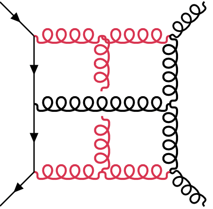
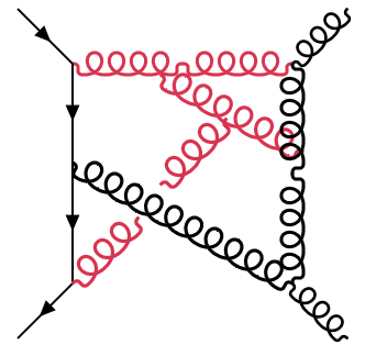
Figure 2: Sample diagrams with quadrupole soft divergences, reinterpreted as tree-level diagrams (black lines) plus virtual gluons (red lines). Diagrams (a) and (b) involve colour correlations between four and three external partons and contribute to the first and second line of eq. (IV), respectively.

The coefficients of the perturbative expansion for the finite remainders

$$\mathbfcal{H}_{\lambda,\text{fin}}=\sum_{\ell\geq 0}\bar{\alpha}_{s}^{\ell}\mathbfcal{H}^{(\ell)}_{\lambda,\text{fin}}$$ (46)

can be obtained according to

$$\mathbfcal{H}_{\lambda,\>\text{fin}}^{(0)} =\mathbfcal{H}_{\lambda}^{(0)}\;,$$

$$\mathbfcal{H}_{\lambda,\>\text{fin}}^{(1)} =\mathbfcal{H}_{\lambda,\>\text{ren}}^{(1)}-\mathbfcal{I}_{1}\mathbfcal{H}_{\lambda,\>\text{ren}}^{(0)}\;,$$

$$\mathbfcal{H}_{\lambda,\>\text{fin}}^{(2)} =\mathbfcal{H}_{\lambda,\>\text{ren}}^{(2)}-\mathbfcal{I}_{2}\mathbfcal{H}_{\lambda,\>\text{ren}}^{(0)}-\mathbfcal{I}_{1}\mathbfcal{H}_{\lambda,\>\text{ren}}^{(1)}\;,$$

$$\mathbfcal{H}_{\lambda,\>\text{fin}}^{(3)} =\mathbfcal{H}_{\lambda,\>\text{ren}}^{(3)}-\mathbfcal{I}_{3}\mathbfcal{H}_{\lambda,\>\text{ren}}^{(0)}-\mathbfcal{I}_{2}\mathbfcal{H}_{\lambda,\>\text{ren}}^{(1)}-\mathbfcal{I}_{1}\mathbfcal{H}_{\lambda,\>\text{ren}}^{(2)}\;,$$ (47)

with

$$\mathbfcal{I}_{1}=\mathbfcal{Z}_{1},\qquad\mathbfcal{I}_{2}=\mathbfcal{Z}_{2}-\mathbfcal{Z}_{1}^{2},\qquad\mathbfcal{I}_{3}=\mathbfcal{Z}_{3}-2\mathbfcal{Z}_{1}\mathbfcal{Z}_{2}+\mathbfcal{Z}_{1}^{3}+\mathbf{\Delta}_{4}^{(3)}\,,$$ (48)

where the $\mathbfcal{Z}_{n}$ are the coefficients of the expansion of $\mathbfcal{Z}$ in $\bar{\alpha}_{s}$ and explicitly read Becher:2009qa ; Caola:2021rqz :

$$\mathbfcal{Z}_{0} =1\,,$$

$$\mathbfcal{Z}_{1} =\frac{\Gamma^{\prime}_{0}}{4\epsilon^{2}}+\frac{\mathbf{\Gamma}_{0}}{2\epsilon}\,,$$

$$\mathbfcal{Z}_{2} =\frac{{\Gamma_{0}^{\prime}}^{2}}{32\epsilon^{4}}+\frac{\Gamma^{\prime}_{0}}{8\epsilon^{3}}\left(\mathbf{\Gamma}_{0}-\frac{3}{2}\beta_{0}\right)+\frac{\mathbf{\Gamma}_{0}}{8\epsilon^{2}}(\mathbf{\Gamma}_{0}-2\beta_{0})+\frac{\Gamma_{1}^{\prime}}{16\epsilon^{2}}+\frac{\mathbf{\Gamma}_{1}}{4\epsilon}\,,$$

$$\mathbfcal{Z}_{3} =\frac{{\Gamma^{\prime}_{0}}^{3}}{384\epsilon^{6}}+\frac{{\Gamma^{\prime}_{0}}^{2}}{64\epsilon^{5}}(\mathbf{\Gamma}_{0}\!-\!3\beta_{0})+\frac{\Gamma_{0}^{\prime}}{32\epsilon^{4}}\left(\mathbf{\Gamma}_{0}\!-\!\frac{4}{3}\beta_{0}\right)\left(\mathbf{\Gamma}_{0}\!-\!\frac{11}{3}\beta_{0}\right)+\frac{\Gamma_{0}^{\prime}\Gamma_{1}^{\prime}}{64\epsilon^{4}}$$

$$\quad+\!\frac{\mathbf{\Gamma}_{0}}{48\epsilon^{3}}(\mathbf{\Gamma}_{0}-\!2\beta_{0})(\mathbf{\Gamma}_{0}-4\beta_{0})\!+\!\frac{\Gamma^{\prime}_{0}}{16\epsilon^{3}}\left(\mathbf{\Gamma}_{1}\!-\!\frac{16}{9}\beta_{1}\right)+\frac{\Gamma_{1}^{\prime}}{32\epsilon^{3}}\left(\mathbf{\Gamma}_{0}\!-\!\frac{20}{9}\beta_{0}\right)+\frac{\mathbf{\Gamma}_{0}\mathbf{\Gamma}_{1}}{8\epsilon^{2}}$$

$$\quad-\!\frac{\beta_{0}\mathbf{\Gamma}_{1}+\beta_{1}\mathbf{\Gamma}_{0}}{6\epsilon^{2}}+\frac{\Gamma_{2}^{\prime}}{36\epsilon^{2}}+\frac{\mathbf{\Gamma}_{2}+\mathbf{\Delta}_{4}^{(3)}}{6\epsilon}\;.$$ (49)

Above we have used

$$\Gamma^{\prime}(\bar{\alpha}_{s})=\frac{\partial\mathbf{\Gamma}(\{p\},\bar{\alpha}_{s},\mu)}{\partial\log\mu}=-\gamma^{\text{K}}\sum_{i}C_{i}=\sum_{\ell\geq 0}\bar{\alpha}_{s}^{\ell+1}\Gamma_{\ell}^{\prime},$$ (50)

with the last equal sign giving the definition of the perturbative coefficients $\Gamma_{\ell}^{\prime}$.
The explicit expression for the perturbative expansions of the cusp anomalous dimension and of the quark (gluon) collinear anomalous dimensions are given in the appendix.

V Checks and exact results

First, we have checked that our results for the lower loop amplitudes are consistent with the literature. In particular, we have compared our tree-level, one-loop and two-loop results for the bare helicity amplitudes for $q\bar{q}\to gg$ in the helicity configurations (19) against the results provided in the ancillary files of ref. Ahmed:2019qtg and find analytical agreement through to weight six. We have also checked that our one-loop expressions for $q\bar{q}\to gg$ and $qg\to qg$ match results obtained with the automated one-loop generator OpenLoops Cascioli:2011va ; Buccioni:2019sur . At the three-loop level, we have verified that the IR singularities of our results for the renormalized helicity amplitudes in eq. (IV) match the pattern predicted by eqs. (37)-(48), which provides a highly non-trivial check. From the high energy limit of our amplitudes we extract the quark and gluon impact factors and find that they are consistent with previous results, which tests lower loop contributions to the renormalized amplitude up to weight six. Moreover, we extract the gluon Regge trajectory and find agreement with previous results, which provides a stringent check of the finite contributions to the three-loop amplitudes presented in this paper. The high energy limit will be described in more detail in the next section.

Our analytic results for the three-loop finite remainders $\mathbfcal{H}_{{\lambda},\>\text{fin}}$ are expressed in terms of harmonic polylogarithms with transcendental weight up to six. Alternatively, these can be converted to a functional basis of logarithms, classical polylogarithms and a few multiple polylogarithms with at most three-fold nested sums Caola:2020dfu . We provide a general conversion table for harmonic polylogarithms up to weight six in the ancillary files of the arXiv submission of this article.

From our results for the process $q\bar{q}\to gg$ we also derive explicit expressions for the helicity amplitudes for $qg\to qg$ scattering, which requires a non-trivial analytical continuation. Details for this procedure are given in ref. Caola:2021rqz . The remaining partonic channels $gg\to q\bar{q}$ and $g\bar{q}\to g\bar{q}$ are not provided explicitly, since they can be obtained by a simple crossing of external legs without any non-trivial analytic continuation. While our results are relatively compact, of the order of 1 megabyte per partonic channel, they are too lengthy to be presented here. We include them in computer-readable format in the ancillary files on arXiv.

In figure 3 we show the finite remainder of the amplitude at different loop orders interfered with the tree-level amplitude for the processes $q\bar{q}\to gg$ and $qg\to qg$. The interferences are averaged (summed) over polarizations and color in the initial (final) state.

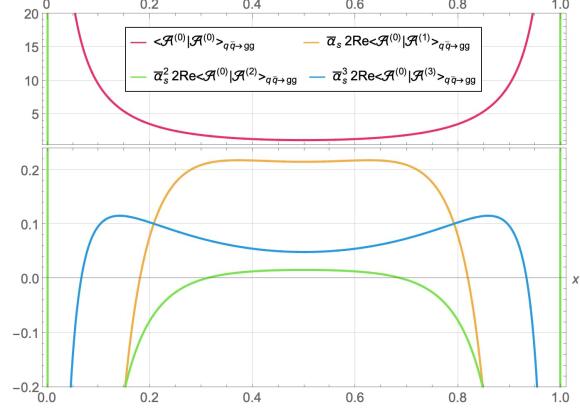
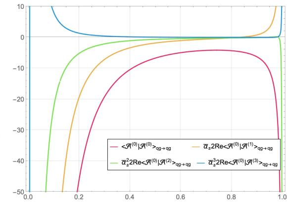
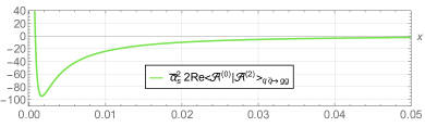
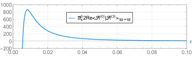
Figure 3: Perturbative amplitudes up to three loops interfered with the tree-level amplitude for $q\bar{q}\to gg$ (panel a) and $qg\to qg$ (panel b) in dependence of $x=-t/s$ . The two-loop contribution to $q\bar{q}\to gg$ diverges to $+\infty$ near $x=0^{+},1^{-}$ (panel c shows details near $x=0^{+}$), while the three-loop contribution to $qg\to qg$ diverges to $-\infty$ near $x=0^{+}$ (panel d).

Additionally, since with the results of this paper all $2\to 2$ partonic channels are now available in three-loop massless QCD, we find it useful to compare virtual corrections for the processes $q\bar{q}\to gg$, $qg\to qg$, $gg\to gg$ and $q\bar{q}\to\bar{Q}Q$. In figure 4, we show the contributions to the squared amplitude at different orders in $\bar{\alpha}_{s}$, normalized by the respective tree-level squared amplitude. Again, we average (sum) over polarization and color in the initial (final) states.

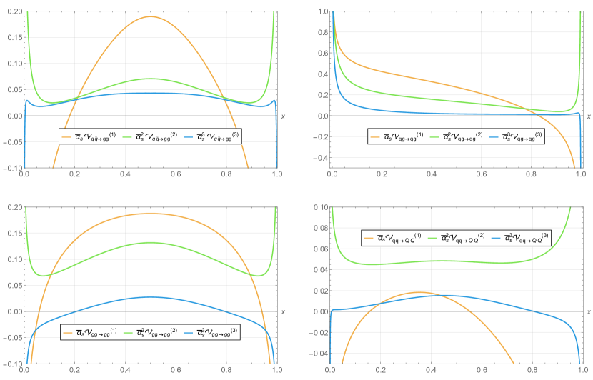
Figure 4: Perturbative expansion of the amplitude squared for the processes $q\bar{q}\to gg$, $qg\to qg$, $gg\to gg$ and $q\bar{q}\to\bar{Q}Q$ as functions of $x=-t/s$. Values are normalized by the tree-level amplitude squared.

Below we define more in detail the quantities we present in the plots.

We rewrite the finite amplitude as a vector in color and helicity space

$$|\mathcal{A}\rangle=4\pi\alpha_{s}\sum_{\ell\geq 0}\bar{\alpha}_{s}^{\ell}\;|\mathcal{A}^{(\ell)}\rangle$$ (51)

and define the contraction between different elements in this vector space as

$$\langle\mathcal{A}^{(\ell)}|\mathcal{A}^{(\ell^{\prime})}\rangle\equiv\mathcal{N}\sum_{i,j,\bm{\lambda}}\mathcal{C}_{i}^{\dagger}\mathcal{C}_{j}|s_{\bm{\lambda}}|^{2}\mathcal{H}^{[i],(\ell)^{*}}_{\bm{\lambda},\rm fin}\mathcal{H}^{[j],(\ell^{\prime})}_{{\bm{\lambda}},\rm fin},$$ (52)

where the factor $4\pi\alpha_{s}$ in eq. (51) replicates the overall normalization of eq. (7). $\mathcal{N}$ is the initial-state color and polarization averaging factor, which depends on the process and takes the following values:

$$\mathcal{N}=\begin{cases}\frac{1}{4N_{c}^{2}}\quad\quad\quad&\text{ for $q\bar{q}\to gg$},\\ \frac{1}{4N_{c}(N_{c}^{2}-1)}\quad&\text{ for $qg\to qg$},\\ \frac{1}{4(N_{c}^{2}-1)^{2}}\quad&\text{ for $gg\to gg$},\\ \frac{1}{4N_{c}^{2}}\quad\quad\quad&\text{ for $q\bar{q}\to\bar{Q}Q$}.\end{cases}$$ (53)

The initial and final state polarization sum runs over all helicity configurations. The color factors $\mathcal{C}_{i}$ and the spinor factors $s_{\bf\lambda}$ are different for the various processes: for $q\bar{q}\to gg$ they are given in eqs. (8) and (23), while for $qg\to qg$ they are obtained by applying the transformation $p_{2}\leftrightarrow p_{3}$ to those of $q\bar{q}\to gg$. For the other two channels $gg\to gg$ and $q\bar{q}\to\bar{Q}Q$, they can be found in refs. Caola:2021izf and Caola:2021rqz respectively.

We expand the squared amplitude normalized by the tree-level contribution in $\bar{\alpha}_{s}$ according to

$$\frac{\langle\mathcal{A}|\mathcal{A}\rangle}{\langle\mathcal{A}^{(0)}|\mathcal{A}^{(0)}\rangle}=\mathcal{V}^{(0)}+\bar{\alpha}_{s}\mathcal{V}^{(1)}+\bar{\alpha}_{s}^{2}\mathcal{V}^{(2)}+\bar{\alpha}_{s}^{3}\mathcal{V}^{(3)}+O(\bar{\alpha}_{s}^{4})$$ (54)

with

$$\mathcal{V}^{(0)} =1,\quad \mathcal{V}^{(1)} =2\frac{\operatorname{Re}\langle\mathcal{A}^{(0)}|\mathcal{A}^{(1)}\rangle}{\langle\mathcal{A}^{(0)}|\mathcal{A}^{(0)}\rangle},\quad$$

$$\mathcal{V}^{(2)} =\frac{\langle\mathcal{A}^{(1)}|\mathcal{A}^{(1)}\rangle}{\langle\mathcal{A}^{(0)}|\mathcal{A}^{(0)}\rangle}+2\frac{\operatorname{Re}\langle\mathcal{A}^{(0)}|\mathcal{A}^{(2)}\rangle}{\langle\mathcal{A}^{(0)}|\mathcal{A}^{(0)}\rangle},\quad \mathcal{V}^{(3)} =2\frac{\operatorname{Re}\langle\mathcal{A}^{(1)}|\mathcal{A}^{(2)}\rangle}{\langle\mathcal{A}^{(0)}|\mathcal{A}^{(0)}\rangle}+2\frac{\operatorname{Re}\langle\mathcal{A}^{(0)}|\mathcal{A}^{(3)}\rangle}{\langle\mathcal{A}^{(0)}|\mathcal{A}^{(0)}\rangle}.$$ (55)

Finally, for the numerical evaluation, we have set $\mu^{2}=s=m_{Z}^{2}$, $\alpha_{s}(\mu)=0.118$, $n_{f}=5$ and $N_{c}=3$.

VI High energy limit

In the high-energy or Regge limit, quantum field theoretic scattering amplitudes become particularly simple and are known to exhibit universal factorization properties. In the following, we consider the process

$$q(p_{1})\;+\;g(p_{2})\;\to\;q(p_{3})\;+\;g(p_{4}),$$ (56)

for which $t$-channel gluon exchanges provide the dominant contribution to the amplitude at high energies. The Regge limit is defined as $s\to\infty$ for fixed scattering angle, that is, $|s|\approx|u|\gg|t|$, where $s=(p_{1}+p_{2})^{2}$, $t=(p_{1}-p_{3})^{2}$, $u=-s-t$ in terms of the momenta in (56). For the variable $x=-t/s$, the Regge limit corresponds to $x\to 0$.

Following the investigation Caron-Huot:2017fxr ; Collins:1977jy , we split the renormalized amplitude into the definite $s\leftrightarrow u$ signature component

$$\mathbfcal{H}_{\mathrm{qg\rightarrow qg,\pm}}=\frac{1}{2}\left.[\mathbfcal{H}_{\mathrm{qg\rightarrow qg}}(s,u)\pm\mathbfcal{H}_{\mathrm{qg\rightarrow qg}}(u,s)\right]\,.$$ (57)

The definite-signature amplitudes $\mathbfcal{H}_{\mathrm{qg\rightarrow qg},+}$ and $\mathbfcal{H}_{\mathrm{qg\rightarrow qg},-}$ are referred to as the even and odd amplitudes. We expand them up to third order in $\bar{\alpha}_{s}$,

$$\mathbfcal{H}_{\mathrm{qg\rightarrow qg},\pm} =\sum_{\ell=0}^{3}\bar{\alpha}_{s}^{\ell}\sum_{k=0}^{\ell}L^{k}\mathbfcal{H}_{\mathrm{qg\rightarrow qg}}^{(\pm,\ell,k)},$$ (58)

where we use for the signature-symmetric logarithm

$$L=-\ln(x)-\frac{i\pi}{2}\approx\frac{1}{2}\left[\ln\left(\frac{-s-i\delta}{-t}\right)+\ln\left(\frac{-u-i\delta}{-t}\right)\right]$$ (59)

and the color operators DelDuca:2013ara ; DelDuca:2014cya are

$$\mathbf{T}_{s}^{2}=(\mathbf{T}_{1}\!+\!\mathbf{T}_{2})^{a}(\mathbf{T}_{1}\!+\!\mathbf{T}_{2})^{a},\;\quad\mathbf{T}_{t}^{2}=(\mathbf{T}_{1}\!+\!\mathbf{T}_{3})^{a}(\mathbf{T}_{1}\!+\!\mathbf{T}_{3})^{a},$$

$$\mathbf{T}_{u}^{2}=(\mathbf{T}_{1}\!+\!\mathbf{T}_{4})^{a}(\mathbf{T}_{1}\!+\!\mathbf{T}_{4})^{a},\;\quad\mathbf{T}_{s-u}^{2}=\frac{1}{2}(\mathbf{T}_{s}^{2}-\mathbf{T}_{u}^{2}).$$ (60)

Here the $\mathbf{T}_{i}$ (i=1,…,4) are assigned according to eq. (IV). Explicitly, we find

(70)

Following ref. Caron-Huot:2017fxr , one can show that the coefficients $\mathbfcal{H}_{\mathrm{qg\rightarrow qg}}^{(-,\ell,k)}$($\mathbfcal{H}_{\mathrm{qg\rightarrow qg}}^{(+,\ell,k)}$) are purely imaginary(real). The $t$-channel exchange of an even number of Reggeons contributes only to $\mathbfcal{H}_{\mathrm{qg\rightarrow qg}}^{(+,\ell,k)}$, while the $t$-channel exchange of an odd number of Reggeons contributes only to $\mathbfcal{H}_{\mathrm{\mathrm{qg\rightarrow qg}}}^{(-,\ell,k)}$. A single Reggeon exchange contributes to the Regge pole contribution, while a multiple Reggeon exchange in general can have non-vanishing contributions to both Regge pole and Regge cuts PhysRev.137.B949 ; Collins:1977jy ; Falcioni:2021dgr ; Falcioni:2021buo . Up to next-to-leading logarithmic (NLL) accuracy, the odd signature amplitude is completely determined by the gluon Regge trajectory and by the so-called quark and gluon impact factors, that describe the interaction of the reggeized gluon with external states. The factorization structure for the odd amplitude becomes more complex in the next-to-next-to-leading logarithmic (NNLL) approximation, as both Regge pole and Regge cut Fadin:2020lam ; Caron-Huot:2017fxr ; DelDuca:2001gu ; DelDuca:2013ara contribute at this order. For the even amplitude, only the Regge cut contributes at the NLL level Caron-Huot:2017fxr and breaks the simple exponential structure already at this logarithmic order. Starting from NNLL, the odd-signature amplitude receives contributions from both Regge pole and Regge cuts. In ref. Falcioni:2021buo , a scheme has been proposed to disentangle the two. As in our previous paper Caola:2021izf , we adopt this scheme to study the high-energy behaviour of $qg\to qg$ to three loops up to NNLL.

Following the framework outlined in Falcioni:2021buo , we assume that, by setting the renormalization scale to $\mu^{2}=-t$, eq. (58) can be written as

$$\mathbfcal{H}_{\mathrm{qg\rightarrow qg},\pm} =\>Z_{q}\;Z_{g}\>e^{L\mathbf{T}_{t}^{2}\tau_{g}}\sum_{\ell=0}^{3}\bar{\alpha}_{s}^{\ell}\sum_{k=0}^{\ell}L^{k}\mathbfcal{O}^{\pm,(\ell)}_{k}\mathbfcal{H}_{\mathrm{qg\rightarrow qg}}^{(0)},$$ (71)

where $\tau_{g}=\sum_{\ell=1}\bar{\alpha}_{s}^{\ell}\tau_{\ell}$ is the gluon Regge trajectory and the factors $Z_{q}=\sum_{\ell=0}\bar{\alpha}_{s}^{\ell}Z_{q}^{(\ell)}$ and $Z_{g}=\sum_{\ell=0}\bar{\alpha}_{s}^{\ell}Z_{g}^{(\ell)}$ capture the collinear poles of the amplitude Caron-Huot:2017fxr for quarks and gluons, respectively. Up to $O(\bar{\alpha}_{s})$ we have

$$Z_{i}^{(0)} =1\,,$$

$$Z_{i}^{(1)} =-C_{i}\gamma^{\text{K}}_{1}\frac{1}{\epsilon^{2}}+4\gamma_{1}^{i}\frac{1}{\epsilon}\,,$$

$$Z_{i}^{(2)} =C_{i}^{2}\frac{(\gamma^{\text{K}}_{1})^{2}}{2\epsilon^{4}}+C_{i}\left[\frac{1}{\epsilon^{3}}\gamma^{\text{K}}_{1}\left(\frac{3\beta_{0}}{4}-4\gamma_{1}^{i}\right)-\frac{\gamma^{\text{K}}_{2}}{\epsilon^{2}}\right]+\frac{2}{\epsilon^{2}}\gamma_{1}^{i}\left(4\gamma_{1}^{i}-\beta_{0}\right)+\frac{8\gamma_{2}^{i}}{\epsilon}\,.$$ (72)

The odd signature color operators $\mathbfcal{O}^{-,(\ell)}_{k}$ contributing at NNLL Caron-Huot:2017fxr are

$$\mathbfcal{O}^{-,(0)}_{0} =1,$$ (73)

$$\mathbfcal{O}^{-,(1)}_{0} =\mathcal{I}^{q}_{1}+\mathcal{I}^{g}_{1},$$

$$\mathbfcal{O}^{-,(2)}_{0} =\left[\mathcal{I}^{q}_{2}+\mathcal{I}^{g}_{2}+\mathcal{I}^{q}_{1}\mathcal{I}^{g}_{1}\right]+\mathcal{B}^{-,\scalebox{0.7}{$(2)$}}[(\mathbf{T}^{2}_{s-u})^{2}-N_{c}^{2}/4],$$

$$\mathbfcal{O}^{-,(3)}_{1} =\mathcal{B}_{1}^{-,\scalebox{0.7}{$(3)$}}\mathbf{T}^{2}_{s-u}[\mathbf{T}^{2}_{t},\mathbf{T}^{2}_{s-u}]+\mathcal{B}_{2}^{-,\scalebox{0.7}{$(3)$}}[\mathbf{T}^{2}_{t},\mathbf{T}^{2}_{s-u}]\mathbf{T}^{2}_{s-u},$$

and the even signature ones contributing at NLL Caron-Huot:2017fxr are

$$\mathbfcal{O}^{+,(1)}_{0} =i\pi\,\mathcal{B}^{+,(1)}\,\mathbf{T}_{s-u}^{2},\;$$

$$\mathbfcal{O}^{+,(2)}_{1} =i\pi\,\mathcal{B}^{+,(2)}\,[\mathbf{T}_{t}^{2},\mathbf{T}_{s-u}^{2}],$$

$$\mathbfcal{O}^{+,(3)}_{2} =i\pi\,\mathcal{B}^{+,(3)}\,[\mathbf{T}_{t}^{2},[\mathbf{T}_{t}^{2},\mathbf{T}_{s-u}^{2}]].$$ (74)

The coefficients $$\mathcal{B}^{\pm,(\ell)}$$ describe the process independent Regge cut contributions Caron-Huot:2013fea ; Caron-Huot:2017fxr ; Falcioni:2021buo and we report them below for convenience. The odd-signature ones are

$$\mathcal{B}^{-,(2)} =\frac{2\pi^{2}}{3}r_{\Gamma}^{2}\left(\frac{3}{\epsilon^{2}}-18\epsilon\zeta_{3}-27\epsilon^{2}\zeta_{4}+\mathcal{O}(\epsilon)\right),$$

$$\mathcal{B}_{1}^{-,(3)} =64\pi^{2}r_{\Gamma}^{3}\left(\frac{1}{48\epsilon^{2}}+\frac{37}{24}\zeta_{3}+\mathcal{O}(\epsilon)\right),$$

$$\mathcal{B}_{2}^{-,(3)} =64\pi^{2}r_{\Gamma}^{3}\left(\frac{1}{24\epsilon^{2}}+\frac{1}{12}\zeta_{3}+\mathcal{O}(\epsilon)\right),$$ (75)

while for even signature one finds

$$\mathcal{B}^{+,(1)} =\,r_{\Gamma}\>\frac{2}{\epsilon},$$

$$\mathcal{B}^{+,(2)} =-\frac{r_{\Gamma}^{2}}{2}\left(\frac{4}{\epsilon^{2}}+72\zeta_{3}\epsilon+108\zeta_{4}\epsilon^{2}+\mathcal{O}(\epsilon^{3})\right),$$

$$\mathcal{B}^{+,(3)} =\frac{r_{\Gamma}^{3}}{6}\bigg{(}\frac{8}{\epsilon^{3}}-176\zeta_{3}-264\zeta_{4}\epsilon-5712\zeta_{5}\epsilon^{2}+\mathcal{O}(\epsilon^{3})\bigg{)}.$$ (76)

$\mathcal{I}^{q}_{\ell}$ and $\mathcal{I}^{g}_{\ell}$ are the perturbative expansion coefficients of the quark and gluon impact factors; they can be extracted from the one- and two-loop calculation Ahmed:2019qtg . The explicit expressions are rather long and are reported to the required orders in $\epsilon$ in appendix B.
With the perturbative expansion of $\tau_{g}$ up to the three-loop order obtained in Caola:2021izf (and provided in appendix B), we have all the ingredients to fully predict the Regge limit of the process $qg\to qg$ through eq. (71), which only requires the tree-level amplitude $\mathcal{H}_{\mathrm{qg\rightarrow qg}}^{(0)}$ as an input.

We find by explicit calculation that the high energy limit of our results for the $qg\to qg$ three-loop amplitude indeed agrees with this prediction and confirms in particular the literature results Caron-Huot:2017fxr ; Falcioni:2021dgr ; Fadin:1996tb ; Blumlein:1998ib ; DelDuca:2021vjq for the gluon Regge trajectory as well as quark and gluon impact factors in QCD. This provides a highly non-trivial test of the universality of high energy factorization in QCD.

VII Conclusions

In this paper, we have presented the three-loop helicity amplitudes for quark-gluon scattering processes in full-color, massless QCD. To perform this calculation, we have made use of various cutting-edge techniques, in particular to handle the Lorentz decomposition of the scattering amplitude and to solve the highly non-trivial system of integration-by-parts identities required to reduce the amplitude to master integrals.

In addition to our previous calculations for the scattering of four quarks and of four gluons, these latest analytical results confirm predictions for the infrared poles of four-point amplitudes in QCD, also for processes with external states in different color representations. Moreover, our results have made it possible to verify the factorization properties of partonic amplitudes in the Regge limit. With this work, all three-loop amplitudes for parton-parton scattering processes are publicly available, providing the virtual corrections to dijet production at N³LO.

Appendix A Anomalous dimensions

In this appendix, we list the perturbative expansions of the cusp anomalous dimension and of the quark and gluon collinear anomalous dimensions,

$$\gamma^{\text{K}}=\sum\limits_{n=0}\left(\frac{\alpha_{s}}{4\pi}\right)^{n+1}\gamma_{n}^{\text{K}},\qquad\gamma^{g/q}=\sum\limits_{n=0}\left(\frac{\alpha_{s}}{4\pi}\right)^{n+1}\gamma_{n}^{q/g}.$$ (77)

The required expansion coefficients of the cusp anomalous dimension read Korchemsky:1987wg ; Moch:2004pa ; Vogt:2004mw

$$\gamma_{0}^{\text{K}} =4\,,$$

$$\gamma_{1}^{\text{K}} =\left(\frac{268}{9}-\frac{4\pi^{2}}{3}\right)C_{A}-\frac{40}{9}\,n_{f}\,,$$

$$\gamma_{2}^{\text{K}} =C_{A}^{2}\left(\frac{490}{3}-\frac{536\pi^{2}}{27}+\frac{44\pi^{4}}{45}+\frac{88}{3}\,\zeta_{3}\right)+C_{A}n_{f}\left(\frac{80\pi^{2}}{27}-\frac{836}{27}-\frac{112}{3}\,\zeta_{3}\right)$$

$$\quad+C_{F}n_{f}\left(32\zeta_{3}-\frac{110}{3}\right)-\frac{16}{27}\,n_{f}^{2}\;.$$ (78)

The required expansion coefficients of the quark collinear anomalous dimension are Moch:2005id

$$\gamma_{0}^{q} =-3C_{F}\,,$$

$$\gamma_{1}^{q} =C_{F}^{2}\left(-\frac{3}{2}+2\pi^{2}-24\zeta_{3}\right)+C_{F}C_{A}\left(-\frac{961}{54}-\frac{11\pi^{2}}{6}+26\zeta_{3}\right)+C_{F}n_{f}\left(\frac{65}{27}+\frac{\pi^{2}}{3}\right),$$

$$\gamma_{2}^{q} =C_{F}^{3}\left(-\frac{29}{2}-3\pi^{2}-\frac{8\pi^{4}}{5}-68\zeta_{3}+\frac{16\pi^{2}}{3}\,\zeta_{3}+240\zeta_{5}\right)$$

$$\mbox{}+C_{F}^{2}C_{A}\left(-\frac{151}{4}+\frac{205\pi^{2}}{9}+\frac{247\pi^{4}}{135}-\frac{844}{3}\,\zeta_{3}-\frac{8\pi^{2}}{3}\,\zeta_{3}-120\zeta_{5}\right)$$

$$\mbox{}+C_{F}C_{A}^{2}\left(-\frac{139345}{2916}-\frac{7163\pi^{2}}{486}-\frac{83\pi^{4}}{90}+\frac{3526}{9}\,\zeta_{3}-\frac{44\pi^{2}}{9}\,\zeta_{3}-136\zeta_{5}\right)$$

$$\mbox{}+C_{F}^{2}n_{f}\left(\frac{2953}{54}-\frac{13\pi^{2}}{9}-\frac{14\pi^{4}}{27}+\frac{256}{9}\,\zeta_{3}\right)$$

$$\mbox{}+C_{F}C_{A}n_{f}\left(-\frac{8659}{729}+\frac{1297\pi^{2}}{243}+\frac{11\pi^{4}}{45}-\frac{964}{27}\,\zeta_{3}\right)$$

$$\mbox{}+C_{F}n_{f}^{2}\left(\frac{2417}{729}-\frac{10\pi^{2}}{27}-\frac{8}{27}\,\zeta_{3}\right)\;,$$ (79)

while for the gluon collinear anomalous dimension Moch:2005tm they read

$$\gamma_{0}^{g} =-\beta_{0}\,,$$

$$\gamma_{1}^{g} =C_{A}^{2}\left(-\frac{692}{27}+\frac{11}{3}\zeta_{2}+2\zeta_{3}\right)+C_{A}n_{f}\left(\frac{128}{27}-\frac{2}{3}\zeta_{2}\right)+2C_{F}n_{f}\,,$$

$$\gamma_{2}^{g} =C_{A}^{3}\left(\frac{-97186}{729}+\frac{6109}{81}\zeta_{2}+\frac{122}{3}\zeta_{3}-\frac{319}{3}\zeta_{4}-\frac{40}{3}\zeta_{2}\zeta_{3}\;-16\zeta_{5}\right)$$

$$\mbox{}+C_{A}^{2}n_{f}\left(\frac{30715}{1458}-\frac{1198}{81}\zeta_{2}+\frac{356}{27}\zeta_{3}+\frac{82}{3}\zeta_{4}\right)-\frac{11}{9}C_{F}n_{f}^{2}-C_{F}^{2}n_{f}$$

$$\mbox{}+C_{A}C_{F}n_{f}\left(\frac{1217}{27}-2\zeta_{2}-\frac{152}{9}\zeta_{3}-8\zeta_{4}\right)+C_{A}n_{f}^{2}\left(-\frac{269}{1458}+\frac{20}{27}\zeta_{2}-\frac{56}{27}\zeta_{3}\right).$$ (80)

Appendix B Impact factors and gluon Regge trajectory

In this appendix we provide expressions relevant for the high-energy limit of the three-loop amplitude discussed in the main text. The expansion coefficients for the quark and gluon impact factors up to two loops read

$$\mathcal{I}^{q}_{1} =\frac{4-\frac{\zeta_{2}}{2}}{N_{c}}+N_{c}\left(\frac{7\zeta_{2}}{2}+\frac{13}{18}\right)-\frac{5n_{f}}{9}$$

$$\quad+\epsilon\bigg{[}N_{c}\left(-\frac{\zeta_{2}}{6}+\frac{10\zeta_{3}}{3}+\frac{40}{27}\right)+\frac{1}{N_{c}}\left(-\frac{3\zeta_{2}}{4}-\frac{7\zeta_{3}}{3}+8\right)+n_{f}\left(\frac{\zeta_{2}}{6}-\frac{28}{27}\right)\bigg{]}$$

$$\quad+\epsilon^{2}\bigg{[}N_{c}\left(-\frac{13\zeta_{2}}{36}+\frac{35\zeta_{4}}{16}-\frac{7\zeta_{3}}{9}+\frac{242}{81}\right)+\frac{1}{N_{c}}\left(-2\zeta_{2}-\frac{47\zeta_{4}}{16}-\frac{7\zeta_{3}}{2}+16\right)$$

$$\quad\quad\quad+n_{f}\left(\frac{5\zeta_{2}}{18}+\frac{7\zeta_{3}}{9}-\frac{164}{81}\right)\bigg{]}$$

$$\quad+\epsilon^{3}\bigg{[}N_{c}\left(-\frac{26\zeta_{2}\zeta_{3}}{3}-\frac{20\zeta_{2}}{27}-\frac{47\zeta_{4}}{48}+\frac{36\zeta_{5}}{5}-\frac{91\zeta_{3}}{54}+\frac{1456}{243}\right)$$

$$\quad\quad\quad+\frac{1}{N_{c}}\left(\frac{7\zeta_{2}\zeta_{3}}{6}-4\zeta_{2}-\frac{141\zeta_{4}}{32}-\frac{31\zeta_{5}}{5}-\frac{28\zeta_{3}}{3}+32\right)$$

$$\quad\quad\quad+n_{f}\left(\frac{14\zeta_{2}}{27}+\frac{47\zeta_{4}}{48}+\frac{35\zeta_{3}}{27}-\frac{976}{243}\right)\bigg{]}$$

$$\quad+\epsilon^{4}\bigg{[}\frac{1}{N_{c}}\left(\frac{7\zeta_{2}\zeta_{3}}{4}-8\zeta_{2}-\frac{47\zeta_{4}}{4}-\frac{93\zeta_{5}}{10}+\frac{49\zeta_{3}^{2}}{18}-\frac{56\zeta_{3}}{3}-\frac{949\pi^{6}}{120960}+64\right)$$

$$\quad\quad\quad+N_{c}\left(\frac{7\zeta_{2}\zeta_{3}}{18}-\frac{121\zeta_{2}}{81}-\frac{611\zeta_{4}}{288}-\frac{31\zeta_{5}}{15}-\frac{91\zeta_{3}^{2}}{18}-\frac{280\zeta_{3}}{81}-\frac{977\pi^{6}}{120960}+\frac{8744}{729}\right)$$

$$\quad\quad\quad+n_{f}\left(-\frac{7\zeta_{2}\zeta_{3}}{18}+\frac{82\zeta_{2}}{81}+\frac{235\zeta_{4}}{144}+\frac{31\zeta_{5}}{15}+\frac{196\zeta_{3}}{81}-\frac{5840}{729}\right)\bigg{]}+\mathcal{O}(\epsilon^{5})\,,$$ (81)

$$\mathcal{I}^{q}_{2} =-\frac{3N_{c}^{2}\zeta_{2}}{2\epsilon^{2}}+N_{c}^{2}\left(\frac{87\zeta_{2}}{4}+\frac{25\zeta_{4}}{16}+\frac{41\zeta_{3}}{9}+\frac{22537}{2592}\right)+\frac{1}{N_{c}^{2}}\left(\frac{21\zeta_{2}}{4}-\frac{83\zeta_{4}}{16}-\frac{15\zeta_{3}}{2}+\frac{255}{32}\right)$$

$$\quad\quad\quad+N_{c}n_{f}\left(-4\zeta_{2}-\frac{23\zeta_{3}}{9}-\frac{650}{81}\right)+\frac{n_{f}}{N_{c}}\left(-\zeta_{2}-\frac{19\zeta_{3}}{9}-\frac{505}{81}\right)+\frac{25n_{f}^{2}}{54}+\frac{19\zeta_{2}}{2}$$

$$\quad\quad\quad-\frac{47\zeta_{4}}{8}-\frac{205\zeta_{3}}{18}+\frac{28787}{648}$$

$$\quad+\epsilon\bigg{[}N_{c}^{2}\left(\frac{161\zeta_{2}\zeta_{3}}{6}+\frac{4055\zeta_{2}}{144}+\frac{587\zeta_{4}}{12}+\frac{49\zeta_{5}}{2}+\frac{898\zeta_{3}}{27}+\frac{911797}{15552}\right)+n_{f}^{2}\left(\frac{140}{81}-\frac{5\zeta_{2}}{18}\right)$$

$$\quad\quad\quad+\frac{1}{N_{c}^{2}}\left(\frac{49\zeta_{2}\zeta_{3}}{6}+\frac{325\zeta_{2}}{16}-\frac{201\zeta_{4}}{16}-3\zeta_{5}-\frac{166\zeta_{3}}{3}+\frac{2157}{64}\right)$$

$$\quad\quad\quad+N_{c}n_{f}\left(-\frac{61\zeta_{2}}{36}-\frac{247\zeta_{4}}{24}-\frac{85\zeta_{3}}{27}-\frac{36031}{972}\right)-\frac{5507\zeta_{3}}{54}+\frac{746543}{3888}$$

$$\quad\quad\quad+\frac{n_{f}}{N_{c}}\left(-\frac{13\zeta_{2}}{4}-\frac{83\zeta_{4}}{24}-\frac{17\zeta_{3}}{27}-\frac{11983}{486}\right)+13\zeta_{2}\zeta_{3}+\frac{115\zeta_{2}}{8}-\frac{1283\zeta_{4}}{48}+\frac{121\zeta_{5}}{2}\bigg{]}$$

$$\quad+\epsilon^{2}\bigg{[}N_{c}^{2}\left(-\frac{3613\zeta_{2}\zeta_{3}}{18}+\frac{5131\zeta_{2}}{864}+\frac{31811\zeta_{4}}{288}+\frac{94\zeta_{5}}{5}-\frac{293\zeta_{3}^{2}}{18}+\frac{12007\zeta_{3}}{648}+\frac{3251\pi^{6}}{120960}\right.$$

$$\quad\quad\quad\left.+\frac{23246941}{93312}\right)+N_{c}n_{f}\left(\frac{625\zeta_{2}\zeta_{3}}{18}+\frac{1475\zeta_{2}}{108}-\frac{779\zeta_{4}}{72}-\frac{143\zeta_{5}}{5}+\frac{1993\zeta_{3}}{81}-\frac{805855}{5832}\right)$$

$$\quad\quad\quad+\frac{1}{N_{c}^{2}}\left(10\zeta_{2}\zeta_{3}+\frac{2287\zeta_{2}}{32}-\frac{5627\zeta_{4}}{64}-\frac{9\zeta_{5}}{2}+\frac{1255\zeta_{3}^{2}}{18}-\frac{6205\zeta_{3}}{24}+\frac{7193\pi^{6}}{120960}+\frac{13575}{128}\right)$$

$$\quad\quad\quad+\frac{n_{f}}{N_{c}}\left(\frac{31\zeta_{2}\zeta_{3}}{9}-\frac{45\zeta_{2}}{4}-\frac{503\zeta_{4}}{144}-\frac{151\zeta_{5}}{15}+\frac{623\zeta_{3}}{81}-\frac{227023}{2916}\right)$$

$$\quad\quad\quad+n_{f}^{2}\left(-\frac{53\zeta_{2}}{54}+\frac{5\zeta_{4}}{48}-\frac{35\zeta_{3}}{27}+\frac{404}{81}\right)+\frac{1613\zeta_{2}\zeta_{3}}{36}+\frac{197\zeta_{2}}{24}-\frac{27175\zeta_{4}}{144}+\frac{791\zeta_{5}}{30}$$

$$\quad\quad\quad+\frac{1621\zeta_{3}^{2}}{18}-\frac{170951\zeta_{3}}{324}+\frac{17\pi^{6}}{70}+\frac{16114247}{23328}\bigg{]}+\mathcal{O}(\epsilon^{3})\,,$$ (82)

and

$$\mathcal{I}^{g}_{1} =N_{c}\left(4\zeta_{2}-\frac{67}{18}\right)+\frac{5n_{f}}{9}+\epsilon\Bigg{[}N_{c}\left(\frac{17\zeta_{3}}{3}+\frac{11\zeta_{2}}{12}-\frac{202}{27}\right)+n_{f}\left(-\frac{\zeta_{2}}{6}+\frac{28}{27}\right)\Bigg{]}$$

$$\quad+\epsilon^{2}\Bigg{[}N_{c}\left(\frac{41\zeta_{4}}{8}+\frac{77\zeta_{3}}{18}+\frac{67\zeta_{2}}{36}-\frac{1214}{81}\right)+n_{f}\left(-\frac{7\zeta_{3}}{9}-\frac{5\zeta_{2}}{18}+\frac{164}{81}\right)\Bigg{]}$$

$$\quad+\epsilon^{3}\Bigg{[}N_{c}\left(-\frac{59\zeta_{2}\zeta_{3}}{6}+\frac{67\zeta_{5}}{5}+\frac{517\zeta_{4}}{96}+\frac{469\zeta_{3}}{54}+\frac{101\zeta_{2}}{27}-\frac{7288}{243}\right)$$

$$\quad\quad\quad+n_{f}\left(-\frac{47\zeta_{4}}{48}-\frac{35\zeta_{3}}{27}-\frac{14\zeta_{2}}{27}+\frac{976}{243}\right)\Bigg{]}$$

$$\quad+\epsilon^{4}\Bigg{[}N_{c}\left(-\frac{\pi^{6}}{4320}-\frac{70\zeta_{3}^{2}}{9}-\frac{77\zeta_{2}\zeta_{3}}{36}+\frac{341\zeta_{5}}{30}+\frac{3149\zeta_{4}}{288}+\frac{1414\zeta_{3}}{81}+\frac{607\zeta_{2}}{81}-\frac{43736}{729}\right)$$

$$\quad\quad\quad+n_{f}\left(\frac{7\zeta_{2}\zeta_{3}}{18}-\frac{31\zeta_{5}}{15}-\frac{235\zeta_{4}}{144}-\frac{196\zeta_{3}}{81}-\frac{82\zeta_{2}}{81}+\frac{5840}{729}\right)\Bigg{]}+\mathcal{O}(\epsilon^{5})\,,$$ (83)

$$\mathcal{I}^{g}_{2} =-\frac{3N_{c}^{2}\zeta_{2}}{2\epsilon^{2}}+N_{c}^{2}\left(\frac{9\zeta_{4}}{4}+\frac{88\zeta_{3}}{9}+\frac{335\zeta_{2}}{18}-\frac{26675}{648}\right)+N_{c}n_{f}\left(\frac{2\zeta_{3}}{9}-\frac{25\zeta_{2}}{9}+\frac{2063}{216}\right)$$

$$\quad\quad\quad+\frac{n_{f}}{N_{c}}\left(2\zeta_{3}-\frac{55}{24}\right)-\frac{25n_{f}^{2}}{162}$$

$$\quad+\epsilon\Bigg{[}N_{c}^{2}\left(22\zeta_{2}\zeta_{3}-39\zeta_{5}+\frac{275\zeta_{4}}{4}+\frac{1865\zeta_{3}}{18}+\frac{3191\zeta_{2}}{72}-\frac{98671}{648}\right)$$

$$\quad\quad\quad+N_{c}n_{f}\left(-\frac{19\zeta_{4}}{2}-\frac{157\zeta_{3}}{9}-\frac{871\zeta_{2}}{108}+\frac{149033}{3888}\right)$$

$$\quad\quad\quad+\frac{n_{f}}{N_{c}}\left(3\zeta_{4}+\frac{19\zeta_{3}}{3}+\frac{\zeta_{2}}{4}-\frac{1711}{144}\right)+n_{f}^{2}\left(\frac{5\zeta_{2}}{54}-\frac{140}{243}\right)\Bigg{]}$$

$$\quad+\epsilon^{2}\Bigg{[}N_{c}^{2}\left(-\frac{4733\pi^{6}}{30240}-\frac{659\zeta_{3}^{2}}{18}-\frac{8987\zeta_{2}\zeta_{3}}{36}-\frac{187\zeta_{5}}{5}+\frac{16103\zeta_{4}}{64}+\frac{121859\zeta_{3}}{324}+\frac{71263\zeta_{2}}{648}\right.$$

$$\quad\quad\quad\left.-\frac{6140957}{11664}\right)+N_{c}n_{f}\left(\frac{781\zeta_{2}\zeta_{3}}{18}+\frac{104\zeta_{5}}{5}-\frac{5803\zeta_{4}}{144}-\frac{5698\zeta_{3}}{81}-\frac{1645\zeta_{2}}{72}+\frac{3197809}{23328}\right)$$

$$\quad\quad\quad+\frac{n_{f}}{N_{c}}\left(-2\zeta_{2}\zeta_{3}+14\zeta_{5}+\frac{19\zeta_{4}}{2}+\frac{197\zeta_{3}}{9}+\frac{55\zeta_{2}}{24}-\frac{42727}{864}\right)$$

$$\quad\quad\quad+n_{f}^{2}\left(-\frac{5\zeta_{4}}{144}+\frac{35\zeta_{3}}{81}+\frac{53\zeta_{2}}{162}-\frac{404}{243}\right)\Bigg{]}+\mathcal{O}(\epsilon^{3})\,.$$ (84)

In order to express the gluon Regge trajectory, we define

$$K(\alpha_{s}(\mu))=-\frac{1}{4}\int_{\infty}^{\mu^{2}}\frac{d\lambda^{2}}{\lambda^{2}}\gamma^{\text{K}}\left(\alpha_{s}(\lambda^{2})\right),$$ (85)

with the perturbative expansion $K=\sum_{\ell\geq 1}K_{\ell}\bar{\alpha}_{s}^{\ell}$. The coefficients up to third order are

$$K_{1} =\frac{\gamma_{0}^{\text{K}}}{\epsilon}\,,$$

$$K_{2} =\frac{2\gamma_{1}^{\text{K}}}{\epsilon}-\frac{\beta_{0}\gamma_{0}^{\text{K}}}{2\epsilon^{2}}\,,$$

$$K_{3} =\frac{16\gamma_{2}^{\text{K}}}{3\epsilon}-\frac{4\beta_{0}\gamma_{1}^{\text{K}}+4\beta_{1}\gamma_{0}^{\text{K}}}{3\epsilon^{2}}+\frac{\beta_{0}^{2}\gamma_{0}^{\text{K}}}{3\epsilon^{3}}\,.$$ (86)

The expansion coefficients of the gluon Regge trajectory $\tau_{\ell}$ can then be written as Caola:2021izf ; Falcioni:2021dgr

$$\tau_{1} =\;e^{\epsilon\gamma_{E}}\frac{\Gamma(1-\epsilon)^{2}\Gamma(1+\epsilon)}{\Gamma(1-2\epsilon)}\frac{2}{\epsilon},$$

$$\tau_{2} =\;K_{2}-\frac{56n_{f}}{27}+N_{c}\left(\frac{404}{27}-2\zeta_{3}\right)+\epsilon\bigg{[}N_{c}\left(\frac{2428}{81}-66\zeta_{3}-\frac{67\zeta_{2}}{9}-3\zeta_{4}\right)$$

$$\quad+n_{f}\left(12\zeta_{3}-\frac{328}{81}+\frac{5\pi^{2}}{27}\right)\bigg{]}+\epsilon^{2}\bigg{[}N_{c}\bigg{(}82\zeta_{5}+\frac{142\zeta_{2}\zeta_{3}}{3}-\frac{4556\zeta_{3}}{27}+\frac{14576}{243}$$

$$\quad-\frac{404\zeta_{2}}{27}-\frac{2321\zeta_{4}}{24}\bigg{)}+n_{f}\left(\frac{680\zeta_{3}}{27}-\frac{1952}{243}+\frac{56\zeta_{2}}{27}+\frac{211\zeta_{4}}{12}\right)\bigg{]}+\mathcal{O}(\epsilon^{3}),$$

$$\tau_{3} =\;K_{3}+N_{c}^{2}\bigg{(}16\zeta_{5}+\frac{40\zeta_{2}\zeta_{3}}{3}-\frac{77\zeta_{4}}{3}-\frac{6664\zeta_{3}}{27}-\frac{3196\zeta_{2}}{81}+\frac{297029}{1458}\bigg{)}+n_{f}^{2}\left(\frac{928}{729}-\frac{128\zeta_{3}}{27}\right)$$

$$\quad+N_{c}n_{f}\left(\frac{412\zeta_{2}}{81}+\frac{2\zeta_{4}}{3}+\frac{632\zeta_{3}}{9}-\frac{171449}{2916}\right)+\frac{n_{f}}{N_{c}}\left(-4\zeta_{4}-\frac{76\zeta_{3}}{9}+\frac{1711}{108}\right)+\mathcal{O}(\epsilon).$$ (87)

Note that since one can expand $\tau_{1}=K_{1}+O(\epsilon)$, the poles of $\tau_{g}$ are given exactly by $K$ defined in eq. (85) (see also ref. Falcioni:2021buo ).

The expressions above are also provided in electronic format in the arXiv submission of this article.

References

• (1) G. Heinrich, Collider Physics at the Precision Frontier, Phys. Rept. 922 (2021) 1–69, [arXiv:2009.00516].
• (2) S. Badger, C. Broennum-Hansen, H. B. Hartanto, and T. Peraro, First look at two-loop five-gluon scattering in QCD, Phys. Rev. Lett. 120 (2018), no. 9 092001, [arXiv:1712.02229].
• (3) S. Abreu, F. Febres Cordero, H. Ita, B. Page, and M. Zeng, Planar Two-Loop Five-Gluon Amplitudes from Numerical Unitarity, Phys. Rev. D97 (2018), no. 11 116014, [arXiv:1712.03946].
• (4) S. Abreu, L. J. Dixon, E. Herrmann, B. Page, and M. Zeng, The two-loop five-point amplitude in $\mathcal{N}=4$ super-Yang-Mills theory, Phys. Rev. Lett. 122 (2019), no. 12 121603, [arXiv:1812.08941].
• (5) S. Abreu, J. Dormans, F. Febres Cordero, H. Ita, and B. Page, Analytic Form of Planar Two-Loop Five-Gluon Scattering Amplitudes in QCD, Phys. Rev. Lett. 122 (2019), no. 8 082002, [arXiv:1812.04586].
• (6) S. Abreu, F. Febres Cordero, H. Ita, B. Page, and V. Sotnikov, Planar Two-Loop Five-Parton Amplitudes from Numerical Unitarity, JHEP 11 (2018) 116, [arXiv:1809.09067].
• (7) S. Abreu, L. J. Dixon, E. Herrmann, B. Page, and M. Zeng, The two-loop five-point amplitude in $\mathcal{N}$ = 8 supergravity, JHEP 03 (2019) 123, [arXiv:1901.08563].
• (8) S. Abreu, B. Page, E. Pascual, and V. Sotnikov, Leading-Color Two-Loop QCD Corrections for Three-Photon Production at Hadron Colliders, JHEP 01 (2021) 078, [arXiv:2010.15834].
• (9) D. Chicherin, T. Gehrmann, J. M. Henn, P. Wasser, Y. Zhang, and S. Zoia, Analytic result for a two-loop five-particle amplitude, Phys. Rev. Lett. 122 (2019), no. 12 121602, [arXiv:1812.11057].
• (10) D. Chicherin, T. Gehrmann, J. M. Henn, P. Wasser, Y. Zhang, and S. Zoia, The two-loop five-particle amplitude in $\mathcal{N}$ = 8 supergravity, JHEP 03 (2019) 115, [arXiv:1901.05932].
• (11) H. A. Chawdhry, M. Czakon, A. Mitov, and R. Poncelet, Two-loop leading-color helicity amplitudes for three-photon production at the LHC, arXiv:2012.13553.
• (12) G. De Laurentis and D. Maître, Two-Loop Five-Parton Leading-Colour Finite Remainders in the Spinor-Helicity Formalism, JHEP 02 (2021) 016, [arXiv:2010.14525].
• (13) H. A. Chawdhry, M. A. Lim, and A. Mitov, Two-loop five-point massless QCD amplitudes within the integration-by-parts approach, Phys. Rev. D 99 (2019), no. 7 076011, [arXiv:1805.09182].
• (14) S. Abreu, J. Dormans, F. Febres Cordero, H. Ita, M. Kraus, B. Page, E. Pascual, M. S. Ruf, and V. Sotnikov, Caravel: A C++ framework for the computation of multi-loop amplitudes with numerical unitarity, Comput. Phys. Commun. 267 (2021) 108069, [arXiv:2009.11957].
• (15) B. Agarwal, F. Buccioni, A. von Manteuffel, and L. Tancredi, Two-loop leading colour QCD corrections to $q\bar{q}\to\gamma\gamma g$ and $qg\to\gamma\gamma q$, JHEP 04 (2021) 201, [arXiv:2102.01820].
• (16) S. Badger, H. B. Hartanto, and S. Zoia, Two-loop QCD corrections to $Wb\bar{b}$ production at hadron colliders, arXiv:2102.02516.
• (17) S. Abreu, F. F. Cordero, H. Ita, B. Page, and V. Sotnikov, Leading-Color Two-Loop QCD Corrections for Three-Jet Production at Hadron Colliders, arXiv:2102.13609.
• (18) B. Agarwal, F. Buccioni, A. von Manteuffel, and L. Tancredi, Two-loop helicity amplitudes for diphoton plus jet production in full color, arXiv:2105.04585.
• (19) H. A. Chawdhry, M. Czakon, A. Mitov, and R. Poncelet, Two-loop leading-colour QCD helicity amplitudes for two-photon plus jet production at the LHC, arXiv:2103.04319.
• (20) S. Badger, C. Brønnum-Hansen, D. Chicherin, T. Gehrmann, H. B. Hartanto, J. Henn, M. Marcoli, R. Moodie, T. Peraro, and S. Zoia, Virtual QCD corrections to gluon-initiated diphoton plus jet production at hadron colliders, arXiv:2106.08664.
• (21) T. Gehrmann, J. M. Henn, and N. A. Lo Presti, Analytic form of the two-loop planar five-gluon all-plus-helicity amplitude in QCD, Phys. Rev. Lett. 116 (2016), no. 6 062001, [arXiv:1511.05409]. [Erratum: Phys.Rev.Lett. 116, 189903 (2016)].
• (22) C. G. Papadopoulos, D. Tommasini, and C. Wever, The Pentabox Master Integrals with the Simplified Differential Equations approach, JHEP 04 (2016) 078, [arXiv:1511.09404].
• (23) T. Gehrmann, J. Henn, and N. Lo Presti, Pentagon functions for massless planar scattering amplitudes, JHEP 10 (2018) 103, [arXiv:1807.09812].
• (24) D. Chicherin, T. Gehrmann, J. Henn, N. Lo Presti, V. Mitev, and P. Wasser, Analytic result for the nonplanar hexa-box integrals, JHEP 03 (2019) 042, [arXiv:1809.06240].
• (25) D. Chicherin and V. Sotnikov, Pentagon Functions for Scattering of Five Massless Particles, JHEP 20 (2020) 167, [arXiv:2009.07803].
• (26) S. Abreu, F. Febres Cordero, H. Ita, M. Klinkert, B. Page, and V. Sotnikov, Leading-color two-loop amplitudes for four partons and a W boson in QCD, JHEP 04 (2022) 042, [arXiv:2110.07541].
• (27) S. Badger, H. B. Hartanto, J. Kryś, and S. Zoia, Two-loop leading colour helicity amplitudes for W±$\gamma$ + j production at the LHC, JHEP 05 (2022) 035, [arXiv:2201.04075].
• (28) H. A. Chawdhry, M. L. Czakon, A. Mitov, and R. Poncelet, NNLO QCD corrections to three-photon production at the LHC, JHEP 02 (2020) 057, [arXiv:1911.00479].
• (29) M. Czakon, A. Mitov, and R. Poncelet, Tour de force in Quantum Chromodynamics: A first next-to-next-to-leading order study of three-jet production at the LHC, arXiv:2106.05331.
• (30) H. A. Chawdhry, M. Czakon, A. Mitov, and R. Poncelet, NNLO QCD corrections to diphoton production with an additional jet at the LHC, arXiv:2105.06940.
• (31) F. Caola, A. Von Manteuffel, and L. Tancredi, Diphoton Amplitudes in Three-Loop Quantum Chromodynamics, Phys. Rev. Lett. 126 (2021), no. 11 112004, [arXiv:2011.13946].
• (32) F. Caola, A. Chakraborty, G. Gambuti, A. von Manteuffel, and L. Tancredi, Three-loop helicity amplitudes for four-quark scattering in massless QCD, JHEP 10 (2021) 206, [arXiv:2108.00055].
• (33) F. Caola, A. Chakraborty, G. Gambuti, A. von Manteuffel, and L. Tancredi, Three-loop gluon scattering in QCD and the gluon Regge trajectory, arXiv:2112.11097.
• (34) P. Bargiela, F. Caola, A. von Manteuffel, and L. Tancredi, Three-loop helicity amplitudes for diphoton production in gluon fusion, arXiv:2111.13595.
• (35) R. N. Lee, A. von Manteuffel, R. M. Schabinger, A. V. Smirnov, V. A. Smirnov, and M. Steinhauser, Fermionic corrections to quark and gluon form factors in four-loop QCD, Phys. Rev. D 104 (2021), no. 7 074008, [arXiv:2105.11504].
• (36) R. N. Lee, A. von Manteuffel, R. M. Schabinger, A. V. Smirnov, V. A. Smirnov, and M. Steinhauser, Quark and gluon form factors in four-loop QCD, arXiv:2202.04660.
• (37) A. Chakraborty, T. Huber, R. N. Lee, A. von Manteuffel, R. M. Schabinger, A. V. Smirnov, V. A. Smirnov, and M. Steinhauser, The $Hb\bar{b}$ vertex at four loops and hard matching coefficients in SCET for various currents, arXiv:2204.02422.
• (38) E. A. Kuraev, L. N. Lipatov, and V. S. Fadin, The Pomeranchuk Singularity in Nonabelian Gauge Theories, Sov. Phys. JETP 45 (1977) 199–204.
• (39) E. A. Kuraev, L. N. Lipatov, and V. S. Fadin, Multi - Reggeon Processes in the Yang-Mills Theory, Sov. Phys. JETP 44 (1976) 443–450.
• (40) I. I. Balitsky and L. N. Lipatov, The Pomeranchuk Singularity in Quantum Chromodynamics, Sov. J. Nucl. Phys. 28 (1978) 822–829.
• (41) G. Falcioni, E. Gardi, N. Maher, C. Milloy, and L. Vernazza, Disentangling the Regge cut and Regge pole in perturbative QCD, arXiv:2112.11098.
• (42) O. Almelid, C. Duhr, and E. Gardi, Three-loop corrections to the soft anomalous dimension in multileg scattering, Phys. Rev. Lett. 117 (2016), no. 17 172002, [arXiv:1507.00047].
• (43) J. M. Henn and B. Mistlberger, Four-Gluon Scattering at Three Loops, Infrared Structure, and the Regge Limit, Phys. Rev. Lett. 117 (2016), no. 17 171601, [arXiv:1608.00850].
• (44) J. Henn, B. Mistlberger, V. A. Smirnov, and P. Wasser, Constructing d-log integrands and computing master integrals for three-loop four-particle scattering, JHEP 04 (2020) 167, [arXiv:2002.09492].
• (45) T. Peraro and L. Tancredi, Physical projectors for multi-leg helicity amplitudes, JHEP 07 (2019) 114, [arXiv:1906.03298].
• (46) T. Peraro and L. Tancredi, Tensor decomposition for bosonic and fermionic scattering amplitudes, Phys. Rev. D 103 (2021), no. 5 054042, [arXiv:2012.00820].
• (47) P. Nogueira, Automatic Feynman graph generation, J.Comput.Phys. 105 (1993) 279–289.
• (48) J. Vermaseren, New features of FORM, math-ph/0010025.
• (49) C. Studerus, Reduze-Feynman Integral Reduction in C++, Comput.Phys.Commun. 181 (2010) 1293–1300, [arXiv:0912.2546].
• (50) A. von Manteuffel and C. Studerus, Reduze 2 - Distributed Feynman Integral Reduction, arXiv:1201.4330.
• (51) S. Laporta, High precision calculation of multiloop Feynman integrals by difference equations, Int.J.Mod.Phys. A15 (2000) 5087–5159, [hep-ph/0102033].
• (52) A. von Manteuffel and R. M. Schabinger, A novel approach to integration by parts reduction, Phys. Lett. B744 (2015) 101–104, [arXiv:1406.4513].
• (53) A. von Manteuffel and R. M. Schabinger, Quark and gluon form factors to four-loop order in QCD: the $N_{f}^{3}$ contributions, Phys. Rev. D95 (2017), no. 3 034030, [arXiv:1611.00795].
• (54) T. Peraro, Scattering amplitudes over finite fields and multivariate functional reconstruction, JHEP 12 (2016) 030, [arXiv:1608.01902].
• (55) T. Peraro, FiniteFlow: multivariate functional reconstruction using finite fields and dataflow graphs, arXiv:1905.08019.
• (56) J. Gluza, K. Kajda, and D. A. Kosower, Towards a Basis for Planar Two-Loop Integrals, Phys. Rev. D 83 (2011) 045012, [arXiv:1009.0472].
• (57) R. M. Schabinger, A New Algorithm For The Generation Of Unitarity-Compatible Integration By Parts Relations, JHEP 01 (2012) 077, [arXiv:1111.4220].
• (58) H. Ita, Two-loop Integrand Decomposition into Master Integrals and Surface Terms, Phys. Rev. D94 (2016), no. 11 116015, [arXiv:1510.05626].
• (59) K. J. Larsen and Y. Zhang, Integration-by-parts reductions from unitarity cuts and algebraic geometry, Phys. Rev. D93 (2016), no. 4 041701, [arXiv:1511.01071].
• (60) J. Böhm, A. Georgoudis, K. J. Larsen, M. Schulze, and Y. Zhang, Complete sets of logarithmic vector fields for integration-by-parts identities of Feynman integrals, Phys. Rev. D 98 (2018), no. 2 025023, [arXiv:1712.09737].
• (61) B. Agarwal and A. Von Manteuffel, On the two-loop amplitude for $gg\to ZZ$ production with full top-mass dependence, PoS RADCOR2019 (2019) 008, [arXiv:1912.08794].
• (62) S. Catani, The Singular behavior of QCD amplitudes at two loop order, Phys.Lett. B427 (1998) 161–171, [hep-ph/9802439].
• (63) G. F. Sterman and M. E. Tejeda-Yeomans, Multiloop amplitudes and resummation, Phys. Lett. B 552 (2003) 48–56, [hep-ph/0210130].
• (64) S. Mert Aybat, L. J. Dixon, and G. F. Sterman, The Two-loop anomalous dimension matrix for soft gluon exchange, Phys. Rev. Lett. 97 (2006) 072001, [hep-ph/0606254].
• (65) S. Mert Aybat, L. J. Dixon, and G. F. Sterman, The Two-loop soft anomalous dimension matrix and resummation at next-to-next-to leading pole, Phys. Rev. D 74 (2006) 074004, [hep-ph/0607309].
• (66) T. Becher and M. Neubert, Infrared singularities of scattering amplitudes in perturbative QCD, Phys. Rev. Lett. 102 (2009) 162001, [arXiv:0901.0722]. [Erratum: Phys.Rev.Lett. 111, 199905 (2013)].
• (67) T. Becher and M. Neubert, On the Structure of Infrared Singularities of Gauge-Theory Amplitudes, JHEP 06 (2009) 081, [arXiv:0903.1126]. [Erratum: JHEP 11, 024 (2013)].
• (68) L. J. Dixon, Matter Dependence of the Three-Loop Soft Anomalous Dimension Matrix, Phys. Rev. D 79 (2009) 091501, [arXiv:0901.3414].
• (69) E. Gardi and L. Magnea, Factorization constraints for soft anomalous dimensions in QCD scattering amplitudes, JHEP 0903 (2009) 079, [arXiv:0901.1091].
• (70) E. Gardi and L. Magnea, Infrared singularities in QCD amplitudes, Nuovo Cim. C 32N5-6 (2009) 137–157, [arXiv:0908.3273].
• (71) G. P. Korchemsky and A. V. Radyushkin, Renormalization of the Wilson Loops Beyond the Leading Order, Nucl. Phys. B 283 (1987) 342–364.
• (72) S. Moch, J. A. M. Vermaseren, and A. Vogt, The Three loop splitting functions in QCD: The Nonsinglet case, Nucl. Phys. B 688 (2004) 101–134, [hep-ph/0403192].
• (73) A. Vogt, S. Moch, and J. A. M. Vermaseren, The Three-loop splitting functions in QCD: The Singlet case, Nucl. Phys. B 691 (2004) 129–181, [hep-ph/0404111].
• (74) R. Brüser, A. Grozin, J. M. Henn, and M. Stahlhofen, Matter dependence of the four-loop QCD cusp anomalous dimension: from small angles to all angles, JHEP 05 (2019) 186, [arXiv:1902.05076].
• (75) J. M. Henn, G. P. Korchemsky, and B. Mistlberger, The full four-loop cusp anomalous dimension in $\mathcal{N}=4$ super Yang-Mills and QCD, JHEP 04 (2020) 018, [arXiv:1911.10174].
• (76) A. von Manteuffel, E. Panzer, and R. M. Schabinger, Cusp and collinear anomalous dimensions in four-loop QCD from form factors, Phys. Rev. Lett. 124 (2020), no. 16 162001, [arXiv:2002.04617].
• (77) V. Ravindran, J. Smith, and W. L. van Neerven, Two-loop corrections to Higgs boson production, Nucl. Phys. B 704 (2005) 332–348, [hep-ph/0408315].
• (78) S. Moch, J. A. M. Vermaseren, and A. Vogt, The Quark form-factor at higher orders, JHEP 08 (2005) 049, [hep-ph/0507039].
• (79) S. Moch, J. Vermaseren, and A. Vogt, Three-loop results for quark and gluon form-factors, Phys. Lett. B 625 (2005) 245–252, [hep-ph/0508055].
• (80) B. Agarwal, A. von Manteuffel, E. Panzer, and R. M. Schabinger, Four-loop collinear anomalous dimensions in QCD and N=4 super Yang-Mills, Phys. Lett. B 820 (2021) 136503, [arXiv:2102.09725].
• (81) E. Remiddi and J. Vermaseren, Harmonic polylogarithms, Int.J.Mod.Phys. A15 (2000) 725–754, [hep-ph/9905237].
• (82) D. Maitre, HPL, a mathematica implementation of the harmonic polylogarithms, Comput. Phys. Commun. 174 (2006) 222–240, [hep-ph/0507152].
• (83) T. Ahmed, J. Henn, and B. Mistlberger, Four-particle scattering amplitudes in QCD at NNLO to higher orders in the dimensional regulator, JHEP 12 (2019) 177, [arXiv:1910.06684].
• (84) F. Cascioli, P. Maierhofer, and S. Pozzorini, Scattering Amplitudes with Open Loops, Phys.Rev.Lett. 108 (2012) 111601, [arXiv:1111.5206].
• (85) F. Buccioni, J.-N. Lang, J. M. Lindert, P. Maierhöfer, S. Pozzorini, H. Zhang, and M. F. Zoller, OpenLoops 2, Eur. Phys. J. C 79 (2019), no. 10 866, [arXiv:1907.13071].
• (86) S. Caron-Huot, E. Gardi, and L. Vernazza, Two-parton scattering in the high-energy limit, JHEP 06 (2017) 016, [arXiv:1701.05241].
• (87) P. D. B. Collins, An Introduction to Regge Theory and High-Energy Physics. Cambridge Monographs on Mathematical Physics. Cambridge Univ. Press, Cambridge, UK, 5, 2009.
• (88) V. Del Duca, G. Falcioni, L. Magnea, and L. Vernazza, High-energy QCD amplitudes at two loops and beyond, Phys. Lett. B 732 (2014) 233–240, [arXiv:1311.0304].
• (89) V. Del Duca, G. Falcioni, L. Magnea, and L. Vernazza, Analyzing high-energy factorization beyond next-to-leading logarithmic accuracy, JHEP 02 (2015) 029, [arXiv:1409.8330].
• (90) S. Mandelstam, Non-regge terms in the vector-spinor theory, Phys. Rev. 137 (Feb, 1965) B949–B954.
• (91) G. Falcioni, E. Gardi, N. Maher, C. Milloy, and L. Vernazza, Scattering amplitudes in the Regge limit and the soft anomalous dimension through four loops, arXiv:2111.10664.
• (92) V. Fadin, Chapter 4: BFKL — Past and Future, pp. 63–90. 2021. arXiv:2012.11931.
• (93) V. Del Duca and E. W. N. Glover, The High-energy limit of QCD at two loops, JHEP 10 (2001) 035, [hep-ph/0109028].
• (94) S. Caron-Huot, When does the gluon reggeize?, JHEP 05 (2015) 093, [arXiv:1309.6521].
• (95) V. S. Fadin, R. Fiore, and M. I. Kotsky, Gluon Regge trajectory in the two loop approximation, Phys. Lett. B 387 (1996) 593–602, [hep-ph/9605357].
• (96) J. Blumlein, V. Ravindran, and W. L. van Neerven, On the gluon Regge trajectory in O alpha-s**2, Phys. Rev. D 58 (1998) 091502, [hep-ph/9806357].
• (97) V. Del Duca, R. Marzucca, and B. Verbeek, The gluon Regge trajectory at three loops from planar Yang-Mills theory, arXiv:2111.14265.