Engines for predictive work extraction from memoryful quantum stochastic processes

Abstract

Quantum information-processing techniques enable work extraction from a system’s inherently quantum features, in addition to the classical free energy it contains. Meanwhile, the science of computational mechanics affords tools for the predictive modeling of non-Markovian classical and quantum stochastic processes. We combine tools from these two sciences to develop a technique for predictive work extraction from non-Markovian stochastic processes with quantum outputs. We demonstrate that this technique can extract more work than non-predictive quantum work extraction protocols, on the one hand, and predictive work extraction without quantum information processing, on the other. We discover a phase transition in the efficacy of memory for work extraction from quantum processes, which is without classical precedent. Our work opens up the prospect of machines that harness environmental free energy in an essentially quantum, essentially time-varying form.

1 Introduction

In the earliest heat engines, a combustible fuel was burned to maintain a temperature gradient between hot and cold heat reservoirs. The second law of thermodynamics holds that no engine can sustainably function with a single reservoir [1, 2, 3, 4]. While thought experiments such as Maxwell’s demon and Szilard’s engine initially appear to defy this law [5], a more complete understanding of thermodynamics resolved the apparent paradox: the resource powering the engine need not be a temperature gradient, but may be any form of free energy—even information [6, 7, 8, 9, 10]. The emerging field of quantum thermodynamics has continued to expand the scope of “fuel” to increasingly general forms of free energy [11, 12]. There has been both theoretical and experimental advancement in constructing engines that can harness the free energy locked up in quantum coherence, over and above classical free energy [13, 14, 15, 16, 17].

The story does not stop there—in addition to static fuel, there is also a dynamical fuel-like resource embodied by complex thermodynamic processes. The framework of computational mechanics in complexity science offers powerful techniques for the characterization and manipulation of stochastic processes. The future behaviour of such a process in general cannot be known perfectly using data from its past. Nevertheless, temporal correlations, i.e., patterns in a process’s behaviour over time, enable prediction. These correlations may even be non-Markovian, whereby the future of a process depend not only on its present, but also on its distant past. Epsilon machines and their quantum extensions [18, 19, 20] perform memory-optimal predictive modelling of stochastic processes. Pattern extractors [16, 21] leverage prediction to extract useful work from the classical free energy present in temporal patterns, exchanging heat with a single bath. However, these predictive engines are not equipped to harness the free energy locked up in quantum degrees of freedom.

1.1 Our contributions

Here, we develop the theoretical prototype for a predictive quantum engine: a machine that charges a battery by feeding on a multipartite quantum system whose parts are temporally correlated via a classical stochastic process. In other words, the engine’s fuel is a classical stochastic process with quantum outputs. It can extract free energy beyond what is accessible to current quantum engines or classical predictive engines. We present a systematic construction of such an engine for arbitrary classical processes and quantum output states. We illustrate its application on example stochastic processes of correlated non-orthogonal qubits. (Fig. 1). We also use this test case to benchmark the performance of our engine against various alternatives, including one without coherent quantum information processing, and one without predictive functionality. Our predictive quantum engine outperforms these alternatives in terms of work output. We show that parametrized processes of correlated non-orthogonal quantum outputs exhibit phase boundaries between parametric regions where memory of past observations can and cannot enhance the work yield—despite the apparently smooth change of memoryful correlations in the process across this boundary. The sudden lack of memory advantage is thus fundamentally thermodynamic (since prediction per se has more freedom than during work extraction) and fundamentally quantum (since classical engines can exploit all the process’s inherent memory). Finally, we generalize the Information Processing Second Law (IPSL) to the quantum regime and derive the fundamental bounds on a quantum pattern engine’s performance.

We begin by introducing stochastic processes as a source of quantum states that will fuel our engine in Section 1.2. Section 2 shows how general interactions with the correlated quantum states induce belief states that enable optimal prediction and work extraction. We then illustrate how a theoretical pattern engine can be constructed in Section 3. The performance of the engine on an example process is then evaluated in Section 4. This leads to the discovery and explanation of the aforementioned phase transition in the efficacy of memory. The fundamental limit of a pattern engine is then derived in Section 5, and finally we draw our conclusion in Section 6.

1.2 What fuels our engine

Typically in quantum information theory, sources of quantum states are assumed to be memoryless, producing independent and identically distributed (IID) quantum states at each discrete time [22, 23]. On the contrary, nature abounds with rich dynamics. To go beyond the IID paradigm, we consider general finite-state sources of quantum states, which can create highly nontrivial correlations across time. Some simple examples are depicted in Fig. 1 Temporally patterned quantum outputs provide fuel for any entity capable of predicting them. Appendix A shows that any change in total correlation among outputs, as quantified by quantum relative entropy, changes nonequilibrium free energy proportionally. Correlations are therefore a source of free energy.

These memoryful sources of quantum states can be represented by a hidden Markov model (HMM) $\mathcal{M}=\Bigl{(}\mathcal{S},\bigl{(}\sigma^{(x)}\bigr{)}_{x\in\mathcal{X}},\bigl{(}T^{(x)}\bigr{)}_{x\in\mathcal{X}}\Bigr{)}$. Here, $\mathcal{S}$ is the HMM’s set of classical latent states. The random variable representing the latent state at time $t$ shall be denoted by $S_{t}$. The transition-matrix element $T^{(x)}_{s,s^{\prime}}=\Pr(S_{t}=s^{\prime},X_{t}=x|S_{t-1}=s)$ represents the probability of transitioning from latent state $s$ to $s^{\prime}$ and emitting the $d$-dimensional quantum state $\sigma^{(x)}$.

For simple HMMs, the memoryful transition structure can be visualized as an annotated directed graph, as in Fig. 1. In this graphical representation, nodes correspond to latent states while the directed edges correspond to latent-state-to-state transitions that produce a certain quantum output with a prescribed probability.

In the example of Fig. 1(a), the ‘biased-coin process’ has only two latent states $s$ and $s^{\prime}$. At each timestep, the latent state switches with probability $p$. The quantum output is $\sigma^{(0)}$ whenever the resultant state is $s$; The quantum output is $\sigma^{(1)}$ whenever the resultant state is $s^{\prime}$. As the switching-probability $p$ approaches 1, the process approaches a period-two output, alternating between the two quantum states $\dots\sigma^{(0)}\otimes\sigma^{(1)}\otimes\sigma^{(0)}\otimes\sigma^{(1)}\dots$. At the other extreme, as $p$ approaches 0, the latent state remains the same for increasingly long epochs that produce long strings of the same quantum output $\dots\sigma^{(0)}\otimes\sigma^{(0)}\otimes\sigma^{(0)}\otimes\sigma^{(0)}\dots$ or $\dots\sigma^{(1)}\otimes\sigma^{(1)}\otimes\sigma^{(1)}\otimes\sigma^{(1)}\dots$ switching between the two behaviors only rarely. More generally, for any $p\in(0,1)$, the process interpolates between these two extreme behaviors.

More complicated HMMs can generate more complex memoryful structure in the quantum-output process. See Fig. 1(b) for a hint of this possible richness.

The HMM specifies the statistics of the non-Markovian classical variables $X_{t}$ across time, which, in turn, induce the quantum outputs indexed by $x\in\mathcal{X}$. The quantum output process is described by the (formal) density operator

$$\rho_{\overleftrightarrow{A}}=\sum_{\overleftrightarrow{x}}\Pr\left(\overleftrightarrow{x}\right)\bigotimes_{t\in\mathbb{Z}}\sigma^{(x_{t})}_{A_{t}},$$ (1)

where each time step $t$ is associated with a unique elementary physical system $A_{t}$, and $\overleftrightarrow{x}=\dots x_{-1}x_{0}x_{1}\dots$ denotes a bi-infinite string over $\mathcal{X}$. The joint quantum state is separable amongst the $A_{t}$s, but can have non-classical correlations in the form of discord [24]. These memoryful quantum sources generalize the kindred ‘classically controlled qubit sources’ of Ref. [25].

Figure 1: Latent-state sources of correlated quantum processes. Each arrow represents a transition between latent states; the label $p:\sigma^{(x)}$ indicates that the transition happens with probability $p$ and produces a quantum state $\sigma^{(x)}$. (a) Perturbed-coin process. (b) 2-1 golden-mean process.

The time-indexed sequence of stochastically-generated quantum outputs $\sigma^{(x_{t})}_{A_{t}}$ of such a process acts as a “fuel tape” that is fed to the engine (Fig. 2) one $A_{t}$ at a time, in a temporal order. If the quantum states could all be stored for a later time, then it would be straightforward to extract all nonequilibrium addition to free energy from the correlated quantum tape, by acting on the full sequence all at once [13], since the multipartite system could then be treated as a single quantum system. Rather, we consider a setting where each elementary physical system has an immediate expiration date—the engine can interact with $A_{t}$ at the present time $t$, and then never again. This time-locality restriction is shared with the information-ratchet [8, 21] and repeated-interaction [23] frameworks. The challenge here is to extract maximal free energy when forced to act only locally and sequentially on the correlated quantum pattern.

Except for being constrained by a stationary finite-state source, the fuel process can be arbitrary in its alphabet size, statistics, and quantum outputs’ finite dimensionality and form—$\sigma^{(x)}$ could be a pure or mixed state over any number of quantum degrees of freedom. Notice that here the form of the set of $\{\sigma^{(x)}\}_{x\in\mathcal{X}}$ does not vary with time, hence the lack of $t$ index. To simplify notation, we will omit the system label $A_{t}$ unless required.

We assume that the source of the fuel tape is known exactly. This entails a complete knowledge of the underlying classical statistics and of the indexed set of quantum states $\{\sigma^{(x)}\}_{x\in\mathcal{X}}$, but not of which specific string $\overleftrightarrow{x}$ is instantiated.

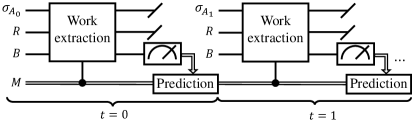
Figure 2: Schematic diagram of a quantum-pattern engine. At each time step, the process will take a quantum system, $\sigma_{A_{t}}$, from the “fuel” tape, reservoir qudit, $R$, battery, $B$, and memory, $M$, as input. The ‘Work extraction’ box should be interpreted as a memory-dependent unitary. States of battery and memory are recycled.

2 Synchronizing to a quantum source

To fully leverage the structure of the pattern, the engine must dynamically incorporate information from past interactions with the elementary quantum systems, so that the engine’s memory becomes correlated with the latent state of the source. This can be done by tracking—within the internal memory $M$ of the engine—an interaction-induced belief state ${\bm{\upeta}}_{t}$ about the latent state of the source.

The type of interaction between engine and fuel at each time can depend on the memory of the engine. The general interaction and observation at time $t$ can be described by a positive operator–valued measure (POVM) on the Hilbert space of the elementary fuel system $A_{t}$; Let $O_{t}$ denote the random variable for the observed outcome thereof.

The optimal belief state ${\bm{\upeta}}_{t}$ at time $t$ is an observation-induced probability distribution over the latent states $\mathcal{S}$ of the source with probability elements

$${\bm{\upeta}}_{t}(s)=\Pr(S_{t}=s|O_{1}\dots O_{t}=o_{1}\dots o_{t})~{}.$$ (2)

This is the best knowledge that a local classical memory can have, as it represents the actual distribution over latent states as one would calculate via Bayes rule. It is convenient to treat ${\bm{\upeta}}_{t}$ as a length-$|\mathcal{S}|$ row vector for linear algebraic manipulation. Given a sequence of observations, what is the probability $P_{t}(x)$ that the source will next produce quantum state $\sigma^{(x)}$? It is $P_{t}(x)={\bm{\upeta}}_{t}T^{(x)}\mathbf{1}$, where $\mathbf{1}$ is the column vector of all ones. The belief state ${\bm{\upeta}}_{t}$ thus determines an expectation of the next quantum state

$$\xi_{t}=\sum_{x\in\mathcal{X}}P_{t}(x)\,\sigma^{(x)}~{},$$ (3)

with more free energy than the local reduced state $\xi_{0}$ of $\rho_{\overleftrightarrow{A}}$. This memory enhancement to free energy is proven in App. B.

The transition rules between these belief states are determined via Bayesian inference, based on the anticipated distribution of the observable $O_{t}$. If the source is known, but no observations have yet been made, then the optimal belief state is simply the stationary distribution over source states: ${\bm{\upeta}}_{0}={\bm{\uppi}}$, which satisfies ${\bm{\uppi}}={\bm{\uppi}}\sum_{x\in\mathcal{X}}T^{(x)}$.
Theorem 1. For any POVM on the quantum state of the system at time $t$, the optimal belief state—about the latent state of the quantum source—updates iteratively according to

$${\bm{\upeta}}_{t}=z_{t}^{-1}\!\sum_{x\in\mathcal{X}}\!\Pr(O_{t}=o_{t}|X_{t}=x,K_{t-1}={\bm{\upeta}}_{t-1})\,{\bm{\upeta}}_{t-1}T^{(x)}$$ (4)

where $K_{t}$ is the random variable for the belief state, and $z_{t}=\sum_{x^{\prime}\in\mathcal{X}}\Pr(O_{t}=o_{t}|X_{t}=x^{\prime},K_{t-1}={\bm{\upeta}}_{t-1})\,{\bm{\upeta}}_{t-1}T^{(x^{\prime})}\mathbf{1}$ is a normalizing factor.

We derive Thm. 1 in Appendix C, generalizing the so-called mixed-state presentation [26, 27, 28, 29, 30].

The probability $\Pr(O_{t}=o_{t}|X_{t}=x,K_{t-1}={\bm{\upeta}}_{t-1})$ appearing in Eq. (4) is typically a straightforward physics calculation of the probability that the observed POVM outcome $o_{t}$ should be obtained, given that the system was prepared as $\sigma^{(x)}$. Conditioning on the previous state of knowledge $K_{t-1}$ is important to the extent that it can influence the choice of POVM applied at time $t$.

Notice that, for each $o$, the update rule for the belief state can be interpreted as a nonlinear return map. If the return map enables prediction, then we have some access to the nonequilibrium free energy in correlations.
Observation 1. Memory can be thermodynamically advantageous when the belief-state update rule has an attractor other than the stationary fixed point ${\bm{\uppi}}$ for at least one observable outcome.

3 Engine construction

The engine is equipped with an internal classical memory $M$ and access to a heat reservoir $R$ at some fixed temperature $T$. Its objective is to extract work by raising the internal energy of a work reservoir or ‘battery’ $B$. To accomplish this, it can bring each system $A_{t}$ closer to its equilibrium state $\gamma=e^{-H/k_{\text{B}}T}/Z$, $k_{\text{B}}$ is Boltzmann’s constant, and $Z=\mathrm{Tr}(e^{-H/k_{\text{B}}T})$ is the associated equilibrium partition function that yields the equilibrium free energy $F=-k_{\text{B}}T\ln Z$. For simplicity of presentation, we assume that each subsystem $A_{t}$ is subject to the same Hamiltonian $H$, but our results generalize in an obvious way if we allow different Hamiltonians for each subsystem. The construction of the pattern engine then requires only the description of the HMM $\mathcal{M}$ and the Hamiltonian $H$.

To harvest the free energy locked up in correlations, the engine’s internal memory should somehow become correlated with the latent state of the source during its energy-harvesting operation. However, directly measuring each quantum system would disturb the state and potentially cost energy. Rather, our engine updates its memory conditioned on the extracted-work value $W_{t}$ at each time. The change in the energy of the battery thus serves as the observable $O_{t}=W_{t}$ for updating the belief state.

At each time step, conditioned on its memory state, the engine performs a work-extraction protocol—a unitary transformation of the composite $A_{t}$, $B$, and $R$ supersystem, designed to transfer energy from $A_{t}$ to $B$.

At best, the work-extraction protocol at time step $t$ would extract all the nonequilibrium addition to free energy $k_{\text{B}}T\text{D}[\rho_{t}^{*}\|\gamma]$ when it acts on a chosen state $\rho_{t}^{*}$, where $\text{D}[\rho\|\gamma]=\mathrm{Tr}(\rho\ln\rho)-\mathrm{Tr}(\rho\ln\gamma)$ is the quantum relative entropy. These are the $\rho^{*}$-ideal work-extraction protocols, which we define as any work-extraction protocol that satisfies the following:

1. When the initial state of the system is $\rho^{*}$, it achieves zero entropy production, transferring on-average all nonequilibrium addition to free energy $k_{\text{B}}T\text{D}[\rho^{*}\|\gamma]$ to a work reservoir, $B$;

2. It conserves energy globally among the reduced states of $A_{t}$, $B$, and $R$ when acting on any eigenstate of $\rho^{*}$.

Our next theorem fully characterizes the set of extracted values and their probabilities for any such protocol (see Appendix D for the derivation).
Theorem 2. Each $\rho^{*}$-ideal work-extraction protocol exhibits at most $d$ distinct extracted-work values. These extracted-work values can be expressed, in terms of the ideal input’s spectral decomposition $\rho^{*}=\sum_{n}\lambda_{n}\ket{\lambda_{n}}\bra{\lambda_{n}}$, as

$$w^{(n)}\coloneqq\bra{\lambda_{n}}H\ket{\lambda_{n}}+k_{\text{B}}T\ln\lambda_{n}-F$$ (5)

with associated probabilities

$$\Pr\bigl{(}W\!=w^{(n)}|\sigma\bigr{)} =\sum_{m}\!\bra{\lambda_{m}}\sigma\ket{\lambda_{m}}\delta_{w^{(n)},w^{(m)}}$$ (6)

This set of values is independent of the actual $d$-dimensional quantum state $\sigma$ input to the protocol, although the input state determines the probabilities of each outcome.

Notably, this yields the probability distribution for work extracted when the protocol optimized for $\rho_{t}^{*}$ actually operates on $\sigma^{(x)}$. Regardless of how the belief state influences the choice of $\rho_{t}^{*}$, we can now leverage Thms. 1 and 2 to rewrite the belief update as

$${\bm{\upeta}}_{t+1} =\frac{\sum_{x\in\mathcal{X}}\sum_{n}\delta_{w_{t+1},w^{(n)}}\bra{\lambda_{n}}\sigma^{(x)}\ket{\lambda_{n}}\,{\bm{\upeta}}_{t}T^{(x)}}{\sum_{n}\delta_{w_{t+1},w^{(n)}}\bra{\lambda_{n}}\xi_{t}\ket{\lambda_{n}}}~{}.$$ (7)

With Eq. (7), the belief-state return maps now reflect the physics of the work-extraction protocol.

From Eqs. (3) and (6), we find that the work-induced transitions between belief states have probabilities

$$\Pr(W_{t+1}=w|K_{t}={\bm{\upeta}}_{t})=\sum_{n}\braket{\lambda_{n}}{\xi_{t}}{\lambda_{n}}\delta_{w,w^{(n)}}~{}.$$ (8)

Finally, to take thermodynamic advantage of this knowledge, the work-extraction protocol at each step is optimized for the expected state, so that $\rho_{t}^{*}=\xi_{t}$. Indeed, extracting all work from the expected state $\xi_{t}$ requires a protocol designed around this expectation [31]. In this case, the denominator in Eq. (7) simplifies to $\sum_{n}\lambda_{n}\,\delta_{w_{t+1},w^{(n)}}$. Similarly, Eq. (8) simplifies to $\sum_{n}\lambda_{n}\,\delta_{w,w^{(n)}}$.

Combining Eqs. (5) and (8), we compute

$$\langle W_{t}\rangle=\sum_{{\bm{\upeta}},w}w\Pr(K_{t-1}\!={\bm{\upeta}})\Pr(W_{t}=w|K_{t-1}\!={\bm{\upeta}})$$ (9)

and find

$$\langle W_{t}\rangle=k_{\text{B}}T\langle\text{D}[\xi_{t}\|\gamma]\rangle_{\Pr(K_{t})}~{}.$$ (10)

Note that the expectation value on the right-hand side is taken over the instantaneous distribution over belief states. The meta-dynamic over belief states thus determines both the transient and asymptotic work-extraction rate. In particular, the stationary distribution over recurrent belief states allows closed-form expressions for the asymptotic work-extraction rate.

Both the belief states and transitions between them derive from the HMM of the known source. Belief states can thus be explicitly represented in the memory $M$ of an autonomous work-harvesting device. The memory states $\{({\bm{\upeta}},\varepsilon)\}_{{\bm{\upeta}},\varepsilon}$ should also store the last measured energy state $\varepsilon$ of the battery. A memory-controlled unitary can implement memory-assisted quantum work extraction, as depicted in the circuit diagram of Fig. 2. Subsequent measurement of the battery state then gives access to the work extracted and allows an autonomous update of the memory, according to the above-outlined rules of Bayesian prediction. This prediction–extraction cycle continues repeatedly, as suggested in Fig. 3.

In short, at every time step, the engine performs both prediction and work-extraction subroutines. The prediction subroutine updates the belief state stored in $M$ via pre-programmed transition rules conditioned on the energy state of $B$. Each unique ${\bm{\upeta}}_{t}$—up to the desired memory resolution—corresponds to a subset of distinguishable states in the memory. The engine’s work-extraction subroutine is conditioned on the memory $M$ and acts on $A_{t}$ with a quantum work-extraction protocol tailored to extract work from $\xi_{t}$.

Figure 3: The protocol proceeds cyclically to fine-tune the belief state.

4 Example processes and alternative approaches

To demonstrate our memory-assisted quantum approach—using a quantum work-extraction protocol designed for the work-observation–induced expected state $\rho_{t}^{*}=\xi_{t}$—we apply it to the quantum perturbed-coin and golden-mean processes depicted in Fig. 1. We compute our engine’s long-term work output from this approach (i) and compare its performance with those of three alternative approaches (ii - iv):

1. memory-assisted quantum, where the quantum work-extraction protocol is optimized for the work-observation–induced expected state $\rho_{t}^{*}=\xi_{t}$;

2. memory-assisted classical, where the protocol, unable to extract work from quantum coherences, is optimized for the energy-dephased version of the expected state $\rho_{t}^{*}=\xi_{t}^{\text{dec}}\coloneqq\sum_{E}\ket{E}\bra{E}\bra{E}\xi_{t}\ket{E}$;

3. memoryless quantum processing, where memory is never updated by observations, and the quantum work-extraction protocol is simply optimized for the time-averaged quantum state $\rho^{*}=\xi_{0}=\sum_{x}{\bm{\uppi}}T^{(x)}\mathbf{1}\,\sigma^{(x)}$; and

4. overcommitment to most probable quantum state, with protocol optimized for $\rho_{t}^{*}=\sigma^{(\text{argmax}_{x}{\bm{\upeta}}_{t}T^{(x)}\mathbf{1})}$.

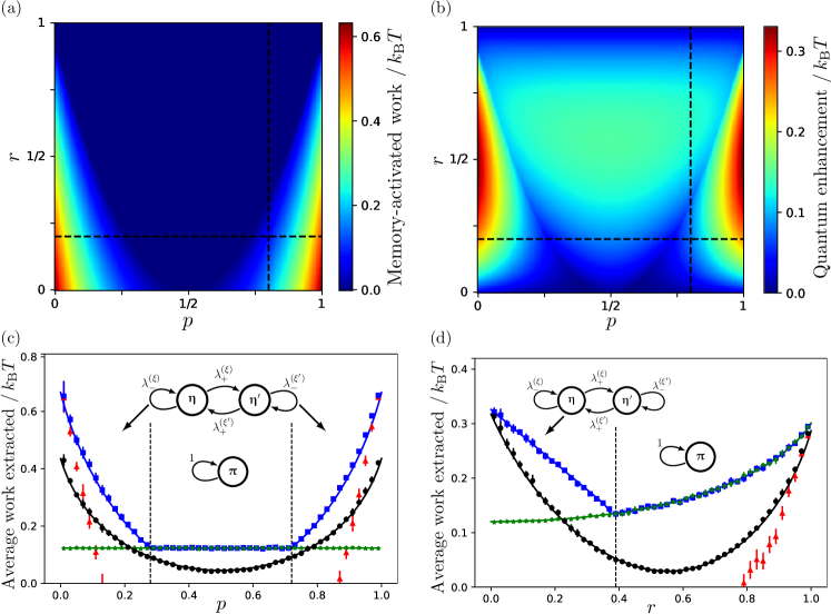
Figure 4: Comparison between average work-extraction rates of various approaches. $p$ characterizes the transition probability between the two latent states of the perturbed-coin process, and $r$ quantifies the overlap between the two quantum outputs. (a) Memory enhancement of work extraction. (b) Quantum enhancement of work extraction. Panels (c) and (d) reveal phase transitions in memory enhancement through cross-sections of parameter space. Analytic results (solid lines) and simulations (markers) are shown. Blue (squares) represents approach (i); black (circles) represents approach (ii); green (stars) represents approach (iii); red (triangles) represents approach (iv).

The asymptotic work-extraction rates $\lim_{t\to\infty}\langle W_{t}\rangle$ from these approaches are compared in Fig. 4, both analytically and with numerical simulations, for the perturbed-coin process. In Fig. 4(a) memory-activated work is defined as the difference between memory-assisted quantum approach (i) and memoryless quantum approach (iii). In Fig. 4(b) quantum enhancement is defined as the difference between memory-assisted quantum approach (i) and memory-assisted classical approach (ii).

In this demonstration, the system extracts work from a sequence of qubits, each with Hamiltonian $H=E_{0}\ket{0}\bra{0}+E_{1}\ket{1}\bra{1}$, with $E_{1}-E_{0}=k_{\text{B}}T$ in this case. At each time step, the source produces one of two nonorthogonal quantum states: $\sigma^{(0)}=\ket{0}\bra{0}$ or $\sigma^{(1)}=\ket{\psi}\bra{\psi}$, where $\ket{\psi}=\sqrt{r}\ket{0}+\sqrt{1-r}\ket{1}$, according to the labeled transition matrices of the perturbed-coin process.

As seen in Fig. 4, our memory-assisted quantum approach (i) always performs at least as well as all other approaches, and strictly outperforms them in many regions of parameter space. In these examples, the ideal input $\rho_{t}^{*}$ is a qubit density matrix with eigenvalues $\lambda_{\pm}^{(\rho_{t}^{*})}$, where $\lambda_{+}^{(\rho_{t}^{*})}\geq\lambda_{-}^{(\rho_{t}^{*})}\geq 0$. Due to Eqs. (5) and (6), we thus expect to observe one of two possible work values, $w^{(\pm)}$ from each distinct belief state.

Approaches (i)-(iii) share some nice features. From Eq. (6), assuming distinct work values $w^{(+)}\neq w^{(-)}$, we find that the probability of observing each possible work value is simply given by the corresponding eigenvalue of the optimal input:

$$\Pr(W_{t+1}=w^{(\pm)}|K_{t}={\bm{\upeta}}_{t})=\lambda_{\pm}^{(\rho_{t}^{*})}~{}.$$ (11)

Combining this with Eq. (5), we find that the rate of work extraction can be expressed as

$$\langle W_{t}\rangle=k_{\text{B}}T\langle\text{D}[\rho_{t}^{*}\|\gamma]\rangle_{\Pr(K_{t})}$$ (12)

for approaches (i)-(iii)—although, notably, both $\rho_{t}^{*}$ and the set of belief states will be different in each approach—with $\rho_{t}^{*}=\xi_{t}$, $\xi_{t}^{\text{dec}}$, and $\xi_{0}$, respectively. The non-negativity of relative entropy thus guarantees the non-negativity of expected work extraction from these three approaches. Note that Eq. (12) is more general than Eq. (10) and allows us to compare work-extraction performance of the three approaches.

Without any memory, the extractable structure is limited to the time-averaged statistical bias of the output [21], which explains why memoryless work extraction varies with $r$ but not $p$. Further details of the analytic solution for expected work extraction can be found in Appendix H.

Our numerical simulations use the quantum work-extraction protocol of Ref. [13] at each time-step, and agree very well with our more general analytical predictions. Indeed, the quantum work-extraction protocol of Ref. [13] provides an example of a $\rho^{*}$-ideal work-extraction protocol, in the limit of many bath interactions. More details can be found in Appendices F and G.

It is tempting to commit to the most likely outcome. However, the overcommitment approach (iv) performs the worst, since any reset operation (to $\gamma$ in this case) with minimal entropy production for a pure-state input leads to infinite heat dissipation when operating on any other input [31, 32]. This translates to infinite negative work extraction $\braket{W_{t}}=-\infty$ in this case of $\rho_{t}^{*}\in\{\ket{0}\!\bra{0},\,\ket{\psi}\!\bra{\psi}\}$. This divergence can alternatively be seen from Eq. (5) as $w^{(-)}\sim\ln\lambda_{-}\to\ln 0=-\infty$. In our numerical simulations, following Ref. [13], this minimal eigenvalue $\lambda_{-}$ is inversely proportional to the number $N$ of bath interactions, so that the overcommitment work penalty diverges as $-k_{\text{B}}T(1-r)\min(p,1-p)\ln N$.

Table 1: Summary of metadynamics in different regimes. The update function shows the nonlinear relationship between $\epsilon_{t}$ and $\epsilon_{t+1}$. The belief evolution shows the evolution of $\epsilon_{t}$ over iterations, which give rise to the corresponding work series, with two possible work values per belief state. The recurrent belief states show the recurrent metadynamic of the different regimes.

4.1 Phase transitions in efficacy of knowledge

Surprisingly, there exists a blue inner region of panel 4(a) where the memoryless quantum approach (iii) achieves the same performance as our memory-assisted quantum approach (i). There exists a sharp phase boundary within which the use of memory does not boost performance. As seen clearly in panels 4(c) and 4(d), the phase boundary exhibits a discontinuity in the first derivative of work extraction with respect to process parametrization. This phase boundary is not unique to the perturbed-coin process and, indeed, also occurs in the 2-1 golden-mean process.

Such phase transitions originate from bifurcations of the attractors of the belief-state update maps. This is illustrated in Table 1, which shows the nonlinear return maps along with the consequences for belief dynamics and work-extraction dynamics. We focus for now on the first two rows of Table 1, which illustrate the nonlinear dynamics of our memory-assisted quantum approach (i), in the memory-apathetic and memory-advantageous regimes, before and after bifurcation respectively.

Recall from Fig. 1(a) that a two-state machine generates the perturbed-coin process. Hence, a scalar $\epsilon_{t}\in[-\tfrac{1}{2},\,\tfrac{1}{2}]$ suffices to describe the time-dependent belief state ${\bm{\upeta}}_{t}=(\tfrac{1}{2}+\epsilon_{t},\,\tfrac{1}{2}-\epsilon_{t})$. The magnitude of this scalar $\epsilon_{t}$ indicates the strength of evidence that the process is in a particular hidden state.

The first column of Table 1 shows the return maps for $\epsilon_{t}\mapsto\epsilon_{t+1}$ induced by either $w^{(+)}$ (red solid graph) or $w^{(-)}$ (blue dashed graph), when the work-extraction protocol is optimized for $\rho_{t}^{*}=\xi_{t}$ (for the first two rows) or $\rho_{t}^{*}=\xi_{t}^{\text{dec}}$ (for the last row). To aid the visual bifurcation and stability analysis, we include a dotted diagonal line with slope one—representing the identity map—and a dotted diagonal line with slope minus one—representing the swap map.

Intersections between a return map and the dotted identity line would indicate a fixed point of the map upon its repeated application. If the magnitude of the slope at the intersection is less than unity, then it is a stable fixed point; if the magnitude of the slope at the intersection is greater than unity, then it is an unstable fixed point. Within the memory-apathetic region of parameter space, Work extraction does not supply enough evidence to nudge an observer out of a state of complete ignorance. In this regime, memory does not enhance quantum work extraction.

At the phase boundary in the process’ parameter space, the fixed point at ${\bm{\uppi}}$ becomes unstable, and new attractors emerge for each map. However, the coexistence of the maps introduces competition between the attractors, as the maps are selected stochastically with probabilities $\lambda_{\pm}$. The two maps (red solid and blue dashed) interact to induce a steady-state metadynamic over recurrent belief states, shown as a Markov process in each row of Table 1’s last column. In this memory-advantageous region, work extraction supplies sufficient evidence to inform an observer about the hidden state of the process, which in turn avails more extractable work.

The elegance of memory-assisted quantum work extraction is reflected in the simple one and two state recurrent memory structures. In comparison, the classical extractor not only harvests less work, but requires more memory to achieve its relatively meager returns. Note the infinite number of recurrent memory states in the classical-processing case, in the last row of Table 1.

5 Fundamental limits of quantum pattern engines

5.1 Initial investment and ideal work-extraction rate

Has our engine performed optimally? To answer this requires some benchmark of optimality. Fortunately, this benchmark is furnished by an appropriate application of the thermodynamic second law.

If we treat the engine’s memory and the multi-partite quantum pattern as a single joint system, we can apply the second law of thermodynamics to (i) bound the maximal possible work extraction, and (ii) discover an initial thermodynamic investment required for the engine to become correlated with the pattern. The transient work investment is apparent in the ‘work series’ column of Table 1. It is a necessary price to harvest work at the optimal steady-state rate.

Let us denote the joint state of a $d_{\text{M}}$-dimensional memory and the length-$L$ pattern as $\rho_{t}^{(\text{M},1:L)}$, with corresponding reduced states of the memory $\rho_{t}^{(\text{M})}$ and of the pattern $\rho_{t}^{(1:L)}$. We will assume that the memory is fully energetically degenerate so that unitary memory updates do not cost energy. Then $\bm{\gamma}=(I/d_{\text{M}})\otimes\gamma^{\otimes L}$ describes the equilibrium state of the joint supersystem. If we denote $W_{t}^{\text{ext}}=\sum_{\ell=1}^{t}W_{\ell}$ as the net work extracted up to time $t$, then the second law of thermodynamics tells us that the reduction in nonequilibrium free energy $\mathcal{F}_{t}^{(\text{M},1:L)}$ upper bounds the expectation value of extracted work [10]:

$$\braket{W_{t}^{\text{ext}}}\leq\mathcal{F}_{0}^{(\text{M},1:L)}-\mathcal{F}_{t}^{(\text{M},1:L)}~{}.$$ (13)

Since the equilibrium free energy is unchanged during our work-extraction process, the change in nonequilibrium free energy is proportional to the change in relative entropy between $\rho_{t}^{(\text{M},1:L)}$ and $\bm{\gamma}$. This relative entropy simplifies further when we invoke several features of our framework: Since the memory is always initialized as $\rho_{0}^{(\text{M})}$, the memory and pattern are initially uncorrelated: $\rho_{0}^{(\text{M},1:L)}=\rho_{0}^{(\text{M})}\otimes\rho_{0}^{(1:L)}$. Through the sequence of deterministic updates, the entropy of the memory is unchanging. Altogether, these features imply that the extractable work is upper bounded by

$$\frac{\braket{W_{t}^{\text{ext}}}}{k_{\text{B}}T}\leq\text{D}[\rho_{0}^{(1:L)}\|\gamma^{\otimes L}]-\text{D}[\rho_{t}^{(1:L)}\|\gamma^{\otimes L}]-\text{I}_{t}~{},$$ (14)

where $\text{I}_{t}=\text{D}[\rho_{t}^{(\text{M},1:L)}\|\rho_{t}^{(\text{M})}\otimes\rho_{t}^{(1:L)}]$ is the mutual information that has built up between the memory and the quantum pattern.

Invoking two more features leads us to a more interpretable version of this result. We note that after $t$ time-steps, the first $t$ subsystems of the pattern have been brought to their equilibrium states, while the other subsystems remain unaltered: $\rho_{t}^{(1:L)}=\gamma^{\otimes t}\otimes\rho_{0}^{(t+1:L)}$. Let $\text{S}(\rho)=-\mathrm{Tr}(\rho\ln\rho)$ denote the von Neumann entropy of $\rho$. If the engine operates on a very long quantum pattern with a von Neumann entropy rate $s_{\text{vN}}\coloneqq\lim_{L\to\infty}\tfrac{1}{L}\text{S}(\rho_{0}^{(1:L)})$, we find that the steady-state work-extraction rate is upper bounded by

$$\frac{\braket{W_{t}}}{k_{\text{B}}T}\,\leq\,\text{S}(\rho_{0}^{(\ell)})-s_{\text{vN}}+\text{D}[\rho_{0}^{(\ell)}\|\gamma]\,\eqqcolon\,\frac{w^{\text{ideal}}}{k_{\text{B}}T}~{},$$ (15)

where the choice of $\ell\in\{1,2,\dots,L\}$ is arbitrary since we assume a stationary quantum pattern. This is a special case of the Quantum Information Processing Second Law (QIPSL), derived as Eq. (77) in Appendix I.

Whenever the input pattern is far from being fully consumed, we find that $\braket{W_{t}^{\text{ext}}}\leq tw^{\text{ideal}}-k_{\text{B}}T\,\text{I}_{t}$. By the information-processing inequality, the investment cost $\text{I}_{t}$ is no more than the quantum excess entropy $\mathcal{E}=\lim_{\ell\to\infty}\text{I}(\rho_{0}^{(1:\ell)};\rho_{0}^{(\ell+1:2\ell)})$, which is the quantum mutual information between the sequences of past and future inputs. However, the engine will only be able to harvest work at the ideal steady-state rate if the memory stores all of the information from past inputs relevant for predicting future inputs, such that $\text{I}_{t}=\mathcal{E}$. Only then will the process be seen at the true entropy rate $s_{\text{vN}}$; otherwise it will appear more random than it really is, with the hidden structure evading extraction.

On the other hand, when the entire pattern has been consumed, $\text{I}_{L}=0$ yet

$$\braket{W_{L}^{\text{ext}}}\leq Lw^{\text{ideal}}-k_{\text{B}}T\mathcal{E}~{}.$$ (16)

The quantum excess entropy $\mathcal{E}$ is a thermodynamic investment for any ideal extractor—even one that operates non-locally. However, for local extractors, this investment must be payed upfront as $\text{I}_{t}$.

In the current framework, it remains an open question whether the knowledge about future inputs $\text{I}_{t}$ attains the fundamental limit of what is knowable $\mathcal{E}$, and whether the work extraction rate $\braket{W_{t}}$ attains $w^{\text{ideal}}$. Perhaps quantum discord prevents local extractors from performing optimally unless they are equipped with quantum memory. Unfortunately, there is no known closed-form solution for the von Neumann entropy rate $s_{\text{vN}}$, even for the simple latent-state models studied here; Accordingly, we cannot analytically evaluate how close our engine is to optimal. Future studies could elucidate the path to optimality, by investigating the work-extraction rate as the agent (a) operates on longer subsequences or (b) explores non-greedy harvesting strategies.

5.2 Energetically-free memory updates in steady state

The initial thermodynamic investment $\text{I}_{t}$ can be associated with the initial nonunitarity of the work-conditioned map on the memory space—the state compression needed for an observer to synchronize (to the extent possible) with the hidden state of the process. However, in the steady state, the work-conditioned maps are unitary for our memory-assisted quantum approach (i). This can be seen in the first two rows of the last column of Table 1: For the perturbed-coin process, the work-induced map is either the identity or swap map on the restriction to the recurrent belief states. These asymptotic memory-update maps are unitary and so can be performed with zero dissipation.

Further investigation is required to determine if the steady-state work-conditioned maps of our approach are always asymptotically unitary for other processes. If not, it may be beneficial to merge the work-extraction and prediction subroutines into a single more sophisticated asymptotically-unitary transformation. We anticipate that the memory updates would then be energetically free in the steady state. This expectation aligns with previous related studies on local work-harvesting pattern extractors in the classical domain, where the ideal pattern extractor—which must be predictive of its input—can update its memory for zero energy cost during steady state work extraction [33, 16, 34, 35].

6 Discussion

We developed the theoretical prototype for a quantum pattern engine: a machine that can adaptively extract useful work from quantum stochastic processes by exploiting knowledge of the temporal patterns they contain. We witnessed that, in the presence of coherence, the memory-assisted quantum approach will always outperform the memory-assisted classical approach. We also demonstrated its advantage over engines that can only harness static quantum resources—although, surprisingly, we found a phase transition marking the onset of memory advantage. It is an open question whether this phase transition coincides with the onset of quantum discord.

In Thm. 1, we found how to update the state of knowledge about any latent-state generator of a quantum process, given any POVM on the current quantum output. In Thm. 2, we found the exact work distribution obtained from any $\rho^{*}$-ideal work-extraction protocol operating on any quantum state. This enabled belief-state updates via observed values of work extraction. Sec. 5 developed the fundamental thermodynamic limits of work extraction from correlated multi-partite quantum systems, which sets the ultimate benchmark for our approach or any alternative.

Despite the advances presented here, many open questions remain for future work.

It is known that measurements themselves can cost some resource, energetic or otherwise [36, 37]. Careful accounting of the resources required for (perfect or imperfect) measurement in our framework would provide a fuller picture of our engine’s performance. Alternatively, it may be possible to use a quantum memory and fully unitary evolution (rather than projective measurements on the battery and subsequent conditional operations on the memory), which would avoid this issue completely.

Although designing the protocol for the observation-induced expected state, $\rho_{t}^{*}=\xi_{t}$, guarantees maximal work extraction locally in time, it remains an interesting open question whether there is a superior steady-state approach that sacrifices short-term work extraction for greater knowledge and long-term returns.

It may be possible to extend our method to more complex quantum processes, e.g., to those with entangled temporal correlations. This would, however, likely require a quantum memory. On the other hand, our method can immediately be adapted to applications where the pattern is spatial instead of temporal (e.g., states of many-body systems), and where the engine is constrained to operate locally on small regions at a time.

7 Acknowledgements

We acknowledge the support of the Singapore Ministry of Education Tier 1 Grants RG146/20 and RG77/22, the NRF2021-QEP2-02-P06 from the Singapore Research Foundation and the Singapore Ministry of Education Tier 2 Grant T2EP50221-0014, the Agency for Science, Technology and Research (A*STAR) under its QEP2.0 programme (NRF2021-QEP2-02-P06) and and the FQXi R-710-000-146-720 Grant “Are quantum agents more energetically efficient at making predictions?” from the Foundational Questions Institute and Fetzer Franklin Fund (a donor-advised fund of Silicon Valley Community Foundation). VN also acknowledges support from the Lee Kuan Yew Endowment Fund (Postdoctoral Fellowship).

Author contributions—PMR and RCH contributed equally to this work. PMR, VN, and MG developed the theoretical formalism. RCH performed the numerical simulations and PMR performed the analytical calculations. All authors contributed to the writing of the manuscript. VN and MG supervised the project.

Appendix A Decomposition of free energy in quantum patterns

Consider a finite portion of the quantum pattern:

$$\rho^{(1:L)}=\mathrm{Tr}_{\mathbb{Z}\setminus\{\ell\}_{1}^{L}}(\rho_{\dots A_{-1}A_{0}A_{1}\dots})~{}.$$ (17)

If each subsystem is non-interacting and the $\ell^{\text{th}}$ subsystem has a reference equilibrium Gibbs state $\gamma^{(\ell)}$, then the nonequilibrium free energy for this portion of the pattern is given by

$$\mathcal{F}^{(1:L)} =F_{\text{eq}}^{(1:L)}+k_{\text{B}}T\text{D}\Bigl{[}\rho^{(1:L)}\|\bigotimes_{\ell=1}^{L}\gamma^{(\ell)}\Bigr{]}$$ (18)

$$=F_{\text{eq}}^{(1:L)}+k_{\text{B}}T\bigl{[}\mathrm{Tr}(\rho^{(1:L)}\ln\rho^{(1:L)})-\sum_{\ell=1}^{L}\mathrm{Tr}(\rho^{(\ell)}\ln\gamma^{(\ell)})\bigr{]}$$ (19)

$$=F_{\text{eq}}^{(1:L)}+k_{\text{B}}T\underbrace{\text{D}[\rho^{(1:L)}\|\bigotimes_{\ell=1}^{L}\rho^{(\ell)}]}_{\text{total correlation}}+k_{\text{B}}T\sum_{\ell=1}^{L}\text{D}[\rho^{(\ell)}\|\gamma^{(\ell)}]~{},$$ (20)

where $F_{\text{eq}}^{(1:L)}$ is the equilibrium free energy.

We recognize that $\text{D}[\rho^{(1:L)}\|\bigotimes_{\ell=1}^{L}\rho^{(\ell)}]$ is the total correlation within the quantum pattern, while $\text{D}[\rho^{(\ell)}\|\gamma^{(\ell)}]$ is the local nonequilibrium addition to free energy. Each of these factors contributes uniquely to the free energy. When operating sequentially on each subsystem, quantum pattern engines must leverage past information to harvest the free energy in the correlations.

In the main text, we suppose each non-interacting subsystem has the same local Hamiltonian, which implies that the reference Gibbs states are also all the same: $\gamma^{(\ell)}=\gamma$. The general decomposition here shows that both quantum and classical correlations contribute to the extractable nonequilium addition to free energy. However, in the main text, the quantum pattern is assumed to be classically-generated, despite having non-orthogonal states. The inter-time quantum correlations are thus restricted to quantum discord, with no inter-time entanglement [24].

Appendix B Memory-enhanced free energy

By self-consistency, the local reduced state of $\rho_{\overleftrightarrow{A}}$ will simply be a probabilistic mixture of $\sigma^{(x)}$ in the form of $\braket{\xi_{t}}_{K_{t}}=\sum_{x\in\mathcal{X}}{\bm{\uppi}}T^{(x)}\mathbf{1}\,\sigma^{(x)}=\xi_{0}$. The predicted quantum state $\xi_{t}$ thus has more free energy than the reduced state on average since

$$\braket{\text{D}[\xi_{t}}{\gamma]}_{K_{t}}-\text{D}[\xi_{0}\|\gamma] =\braket{\text{D}[\xi_{t}}{\gamma]}_{K_{t}}-\text{D}[\braket{\xi_{t}}_{K_{t}}\|\gamma]$$ (21)

$$=S(\braket{\xi_{t}}_{K_{t}})-\braket{S(\xi_{t})}_{K_{t}}$$ (22)

$$\geq 0~{}.$$ (23)

Thus,

$$\braket{\text{D}[\xi_{t}}{\gamma]}_{K_{t}}\geq\text{D}[\xi_{0}\|\gamma]~{},$$ (24)

and so more work can be extracted on average when memory is leveraged to predict sequential quantum states. The non-negativity of Eq. (23) can be seen either from the convexity of relative entropy in Eq. (21) or from the concavity of entropy in Eq. (22).

A nearly identical argument also shows that the classically predicted state has more free energy than the average classical state: $\braket{\text{D}[\xi_{t}^{\text{dec}}}{\gamma]}_{K_{t}}\geq\text{D}[\xi_{0}^{\text{dec}}\|\gamma]$, where the states of knowledge $K_{t}$ are now the classically induced ones.

Appendix C Synchronizing to a memoryful quantum source

Inferring the latent state of a known memoryful quantum source allows maximal work extraction when operating serially on the quantum states of the process. The optimal state of knowledge, given a sequence of observations $o_{1}o_{2}\dots o_{t}$ obtained via interventions on the sequence of quantum systems $\sigma^{(x_{1})},\sigma^{(x_{2})},\dots\sigma^{(x_{t})}$ is the conditional probability distribution induced by these interventions,

$${\bm{\upeta}}_{t}:=\Pr(S_{t}|O_{1}\dots O_{t}=o_{1}\dots o_{t},S_{0}\sim{\bm{\uppi}})~{}.$$ (25)

The last condition $S_{0}\sim{\bm{\uppi}}$ means that the initial latent state of the generator is distributed as ${\bm{\uppi}}$. This can be rewritten as ${\bm{\upeta}}_{t}=\sum_{s}{\bm{\uppi}}(s)\Pr(S_{t}|O_{1}\dots O_{t}=o_{1}\dots o_{t},S_{0}=s)$ for $t>0$. Recall that ${\bm{\uppi}}={\bm{\uppi}}\sum_{x\in\mathcal{X}}T^{(x)}$ is the stationary distribution over the states of the generator. Thus, ${\bm{\upeta}}_{0}={\bm{\uppi}}$.

If we introduce a new random variable $K_{t}$ to denote the optimally updated state of knowledge about the latent state of the pattern generator, then we can replace the condition $S_{t-1}\sim{\bm{\upeta}}_{t-1}$ with $K_{t-1}={\bm{\upeta}}_{t-1}$. The condition on the state of knowledge is relevant to the extent that the choice of POVM is influenced by the state of knowledge. We remind the reader that in our framework the POVM on the current quantum output is chosen as a function of the state of knowledge $K_{t}$.

Note that the current quantum output only depends on the current latent state of the process. Accordingly, the next observation—which is the outcome of the POVM on the current quantum output—is conditionally independent of all previous outputs, given the current latent state and given the state of knowledge induced by all previous outputs.

We will now show that the optimal state of knowledge is recursive. I.e., we will show that:

$${\bm{\upeta}}_{t} =\Pr(S_{t}|O_{t}=o_{t},S_{t-1}\sim{\bm{\upeta}}_{t-1})~{}.$$ (26)

This follows from marginalizing over intervening latent states, employing Bayes’ rule, and recognizing that the belief state ${\bm{\upeta}}_{t}$ is a function of the observations up to that time $o_{1}\dots o_{t}$. Starting from Eq. (25), we find:

$${\bm{\upeta}}_{t} :=\Pr(S_{t}|O_{1}\dots O_{t}=o_{1}\dots o_{t},S_{0}\sim{\bm{\uppi}})$$

$$=\sum_{s}\Pr(S_{t},S_{t-1}=s|O_{1}\dots O_{t}=o_{1}\dots o_{t},S_{0}\sim{\bm{\uppi}})$$ (27)

$$=\frac{\sum_{s}\Pr(S_{t},O_{t}=o_{t},S_{t-1}=s|O_{1}\dots O_{t-1}=o_{1}\dots o_{t-1},S_{0}\sim{\bm{\uppi}})}{\Pr(O_{t}=o_{t}|O_{1}\dots O_{t-1}=o_{1}\dots o_{t-1},S_{0}\sim{\bm{\uppi}})}$$ (28)

$$=\frac{\sum_{s}\Pr(S_{t-1}=s|O_{1}\dots O_{t-1}=o_{1}\dots o_{t-1},S_{0}\sim{\bm{\uppi}})\Pr(S_{t},O_{t}=o_{t}|O_{1}\dots O_{t-1}=o_{1}\dots o_{t-1},S_{0}\sim{\bm{\uppi}},S_{t-1}=s)}{\sum_{s^{\prime}}\Pr(O_{t}=o_{t},S_{t-1}=s^{\prime}|O_{1}\dots O_{t-1}=o_{1}\dots o_{t-1},S_{0}\sim{\bm{\uppi}})}$$ (29)

$$=\frac{\sum_{s}{\bm{\upeta}}_{t-1}(s)\Pr(S_{t},O_{t}=o_{t}|K_{t-1}={\bm{\upeta}}_{t-1},S_{t-1}=s)}{\sum_{s^{\prime}}{\bm{\upeta}}_{t-1}(s^{\prime})\Pr(O_{t}=o_{t}|K_{t-1}={\bm{\upeta}}_{t-1},S_{t-1}=s^{\prime})}$$ (30)

$$=\Pr(S_{t}|O_{t}=o_{t},K_{t-1}={\bm{\upeta}}_{t-1})~{}.$$ (31)

Hence, we have obtained Eq. (26) from Eq. (25) as promised.

Figure 5: Bayesian network showing the structure of conditional independencies among latent states $S_{t}$ of the quantum source, the type $X_{t}$ of quantum state produced, the observable $O_{t}$ attained from interaction, and the state of knowledge $K_{t}$ that influences the work extraction protocol.

Further manipulations, using the rules of probability and the conditional independencies indicated in the Bayesian network depicted in Fig. 5, allow us to express the optimal state of knowledge in terms of both conditional work distributions and simple linear algebraic manipulations of the generative HMM representing the memoryful source. We find

$${\bm{\upeta}}_{t} =\Pr(S_{t}|O_{t}=o_{t},S_{t-1}\sim{\bm{\upeta}}_{t-1})$$ (32)

$$=\sum_{x\in\mathcal{X}}\Pr(S_{t},X_{t}=x|O_{t}=o_{t},S_{t-1}\sim{\bm{\upeta}}_{t-1})$$ (33)

$$=\sum_{x\in\mathcal{X}}\Pr(X_{t}=x|O_{t}=o_{t},S_{t-1}\sim{\bm{\upeta}}_{t-1})\Pr(S_{t}|X_{t}=x,S_{t-1}\sim{\bm{\upeta}}_{t-1})$$ (34)

$$=\sum_{x\in\mathcal{X}}\Pr(X_{t}=x|O_{t}=o_{t},S_{t-1}\sim{\bm{\upeta}}_{t-1})\frac{{\bm{\upeta}}_{t-1}T^{(x)}}{{\bm{\upeta}}_{t-1}T^{(x)}\mathbf{1}}$$ (35)

$$=\frac{\sum_{x\in\mathcal{X}}\Pr(X_{t}=x,O_{t}=o_{t}|S_{t-1}\sim{\bm{\upeta}}_{t-1}){\bm{\upeta}}_{t-1}T^{(x)}/{\bm{\upeta}}_{t-1}T^{(x)}\mathbf{1}}{\sum_{x^{\prime}\in\mathcal{X}}\Pr(X_{t}=x^{\prime},O_{t}=o_{t}|S_{t-1}\sim{\bm{\upeta}}_{t-1})}$$ (36)

$$=\frac{\sum_{x\in\mathcal{X}}\Pr(O_{t}=o_{t}|X_{t}=x,S_{t-1}\sim{\bm{\upeta}}_{t-1})\,{\bm{\upeta}}_{t-1}T^{(x)}}{\sum_{x^{\prime}\in\mathcal{X}}\Pr(O_{t}=o_{t}|X_{t}=x^{\prime},S_{t-1}\sim{\bm{\upeta}}_{t-1})\,{\bm{\upeta}}_{t-1}T^{(x^{\prime})}\mathbf{1}}~{}.$$ (37)

C.1 Using this to build a predictive work-extraction engine

Rather than repeatedly calculating these ideal belief states on the fly for a specific realization of the process, we can alternatively systematically build up the set of all such belief states, together with the observation-induced transitions among them, to inform the design of an autonomous engine. There will be both a set of transient belief states and a set of recurrent belief states. Both of these sets may be either finite or infinite. In the case that only finitely many belief states are induced by observations, we can explicitly build out the transition structure among them. If there are infinitely many such states, then we would need to truncate unlikely states in the design of our finite physical engine [28].

The physical memory system of our proposed engine should have at least one distinguishable state corresponding to every observation-induced belief state. In fact, the memory must encode both the belief state and the most recent energy of the battery, so that conditioning on the new state of the battery is sufficient to supply the change in battery energy. These will likely be encoded with some finite precision, to avoid storing real numbers. Conditioned on the state of the memory encoding ${\bm{\upeta}}$, the work extraction protocol will operate jointly on the quantum system, thermal reservoirs, and battery, to optimally extract work from the expected state $\xi=\sum_{x\in\mathcal{X}}{\bm{\upeta}}T^{(x)}\mathbf{1}\sigma^{(x)}$.

The subsequently observed work value $w$ uniquely updates the memory from the state encoding ${\bm{\upeta}}$ to the state encoding ${\bm{\upeta}}^{\prime}=\frac{\sum_{x\in\mathcal{X}}\Pr(W_{t}=w|X_{t}=x,S_{t-1}\sim{\bm{\upeta}})\,{\bm{\upeta}}T^{(x)}}{\sum_{x^{\prime}\in\mathcal{X}}\Pr(W_{t}=w|X_{t}=x^{\prime},S_{t-1}\sim{\bm{\upeta}})\,{\bm{\upeta}}T^{(x^{\prime})}\mathbf{1}}$. Once the next quantum system arrives, the predictive quantum work extraction cycle begins again.

Appendix D Proof of Thm. 2: Work extraction, in the limit of zero entropy production

Work extraction in the limit of zero entropy production is important since it extracts all extractable work from a quantum state. It thus indicates the best possible scenario, against which other efforts can be compared.

In the limit of zero-entropy-production work extraction from $\rho^{*}$, the net unitary time evolution of the system–battery–baths supersystem must take a special form. In particular, the state of the battery will change deterministically when the initial state of the system is an eigenstate $\ket{\lambda_{n}}$ of $\rho^{*}=\sum_{n}\lambda_{n}\ket{\lambda_{n}}\bra{\lambda_{n}}$, almost-surely independent of the initial realization of the reservoirs. This implies that the net unitary time evolution will be of the form

$$U=\sum_{\varepsilon,n,r}\Bigl{(}\ket{\varepsilon+w^{(n)}}\otimes\ket{f_{\varepsilon}(n,r)}\Bigr{)}\Bigl{(}\bra{\varepsilon}\otimes\bra{\lambda_{n}}\otimes\bra{r}\Bigr{)}$$ (38)

for some $w^{(n)}\in\mathbb{R}$. Above, $\ket{\varepsilon}$ and $\ket{\varepsilon+w^{(n)}}$ are energy eigenstates of the work reservoir, while $\ket{r}$ is an energy eigenstate of the thermal baths. It will be useful in the following to note that $\braket{f_{\varepsilon}(n,r)}{f_{\varepsilon}(n^{\prime},r^{\prime})}=\delta_{n,n^{\prime}}\delta_{r,r^{\prime}}$ since unitary operations map orthogonal states to orthogonal states

The form of the unitary Eq. (38) effectively assumes that the energy of the battery is well above its ground state. Some interesting nuances have recently been explored for batteries close to their ground state (see, e.g., Ref. [38]), which would affect the statistics of the work-extraction values, but we avoid that regime here to instead focus on the best-possible scenario.

One way to determine $w^{(n)}$ is via the initial-state dependence of entropy production. Let $\braket{\Sigma}_{\rho}$ denote the expectation value for entropy production, given initial system-state $\rho$, under the fixed work-extraction protocol optimized for $\rho^{*}$. In our case with a single heat bath at temperature $T$, the expected entropy production can be defined as usual as $\braket{\Sigma}_{\rho}=\bigl{(}\braket{\tilde{W}}_{\rho}-\Delta\mathcal{F}_{t}\bigr{)}/T$. This is the entropy production for a fixed protocol operating on the initial state $\rho$, where $\mathcal{F}_{t}$ is the nonequilibrium free energy at time $t$, while $\Delta\mathcal{F}_{t}$ is the change in nonequilibrium free energy over the course of the protocol, and $\tilde{W}$ is the work exerted, which is just the negative of the extractable work [10]. Since all initial states map to $\gamma$ by the end of the work-extraction protocol, we know from Ref. [31] that

$$\braket{\Sigma}_{\sigma}-\braket{\Sigma}_{\rho^{*}}=k_{\text{B}}\text{D}[\sigma\|\rho^{*}]~{}.$$ (39)

In this case, $\braket{\Sigma}_{\rho^{*}}=0$ and $T\braket{\Sigma}_{\sigma}=\braket{\tilde{W}}_{\sigma}-\Delta\mathcal{F}_{t}=\braket{\tilde{W}}_{\sigma}+k_{\text{B}}T\text{D}[\sigma\|\gamma]$. Hence, with $\beta=(k_{\text{B}}T)^{-1}$,

$$\beta\braket{\tilde{W}}_{\sigma} =\text{D}[\sigma\|\rho^{*}]-\text{D}[\sigma\|\gamma]$$ (40)

$$=\mathrm{Tr}(\sigma\ln\gamma)-\mathrm{Tr}(\sigma\ln\rho^{*})~{}.$$ (41)

In particular, let $\sigma=\ket{\lambda_{n}}\bra{\lambda_{n}}$, and note that $\ln\gamma=\ln(e^{-\beta H}/Z)=\beta(F-H)$. This yields $\braket{\tilde{W}}_{\ket{\lambda_{n}}\bra{\lambda_{n}}}=F-\braket{\lambda_{n}}{H}{\lambda_{n}}-k_{\text{B}}T\ln\lambda_{n}$. The deterministic work-extraction value, given initial pure state $\ket{\lambda_{n}}$, must be the same as its expected value $w^{(n)}=-\braket{\tilde{W}}_{\ket{\lambda_{n}}\bra{\lambda_{n}}}$, and is thus given by

$$w^{(n)}=\braket{\lambda_{n}}{H}{\lambda_{n}}+k_{\text{B}}T\ln\lambda_{n}-F~{}.$$ (42)

The probability of obtaining the work-extraction value $w$, given any input state $\sigma=\sum_{n,m}\ket{\lambda_{n}}\bra{\lambda_{m}}\braket{\lambda_{n}}{\sigma}{\lambda_{m}}$, can be calculated as

$$\Pr(W=w|\sigma) =\mathrm{Tr}\Bigl{[}\bigl{(}\ket{\varepsilon_{0}+w}\bra{\varepsilon_{0}+w}\otimes I\bigr{)}U\bigl{(}\ket{\varepsilon_{0}}\bra{\varepsilon_{0}}\otimes\sigma\otimes\ket{r}\bra{r}\bigr{)}U^{\dagger}\Bigr{]}$$ (43)

$$=\sum_{n,m}\braket{\lambda_{n}}{\sigma}{\lambda_{m}}\mathrm{Tr}\Bigl{[}\bigl{(}\ket{\varepsilon_{0}+w}\bra{\varepsilon_{0}+w}\otimes I\bigr{)}U\bigl{(}\ket{\varepsilon_{0}}\bra{\varepsilon_{0}}\otimes\ket{\lambda_{n}}\bra{\lambda_{m}}\otimes\ket{r}\bra{r}\bigr{)}U^{\dagger}\Bigr{]}$$ (44)

$$=\sum_{n,m}\braket{\lambda_{n}}{\sigma}{\lambda_{m}}\mathrm{Tr}\Bigl{[}\bigl{(}\ket{\varepsilon_{0}+w}\bra{\varepsilon_{0}+w}\otimes I\bigr{)}\bigl{(}\ket{\varepsilon_{0}+w^{(n)}}\otimes\ket{f_{\varepsilon_{0}}(n,r)}\bigr{)}\bigl{(}\bra{\varepsilon_{0}+w^{(m)}}\otimes\bra{f_{\varepsilon_{0}}(m,r)}\bigr{)}\Bigr{]}$$ (45)

$$=\sum_{n,m}\braket{\lambda_{n}}{\sigma}{\lambda_{m}}\delta_{w,w^{(n)}}\delta_{w,w^{(m)}}\braket{f_{\varepsilon_{0}}(m,r)}{f_{\varepsilon_{0}}(n,r)}$$ (46)

$$=\sum_{n,m}\braket{\lambda_{n}}{\sigma}{\lambda_{m}}\delta_{w,w^{(n)}}\delta_{w,w^{(m)}}\delta_{n,m}$$ (47)

$$=\sum_{n}\braket{\lambda_{n}}{\sigma}{\lambda_{n}}\delta_{w,w^{(n)}}$$ (48)

independent of the initial energy state of the battery $\ket{\varepsilon_{0}}$, and almost-surely independent of the initial realization $\ket{r}$ of the thermal reservoirs in the probability theoretic sense. We see that $\Pr(W=w|\sigma)=0$ unless $w\in\{w^{(n)}\}_{n}$. The probability distribution over these allowed work-extraction values is

$$\Pr(W=w^{(n)}|\sigma) =\sum_{m}\braket{\lambda_{m}}{\sigma}{\lambda_{m}}\delta_{w^{(n)},w^{(m)}}~{}.$$ (49)

When there is some entropy production, the probability density of work extraction will have more diffuse peaks. However, for sufficiently low entropy production, the peaks will still be well separated and, so, effectively discrete for the purpose of Bayesian updating.

The above derivation is valid whether or not $\rho^{*}$ has degenerate eigenvalues. Notably, the above sums are taken over the eigenstates and their associated eigenvalues, rather than summing over the eigenvalues directly.

Appendix E Power and inefficiency at rapid operation

It is a familiar concept in the design of any engine: that maximal thermodynamic efficiency requires sufficiently slow operation. Clearly, this has implications for the power output of the engine [39, 40]. However, the relaxation timescales of an engine depend on particular material properties of the system and baths, as well as the particular interaction Hamiltonian, so there is no implementation-independent timescale that determines the practical operation speed of an engine.

Nevertheless, we can apply rather general principles to assess how power typically scales with increasingly fast operation. For example, under assumptions of a Lindblad master equation, there will be a contribution to entropy production (and a corresponding decrease in extracted work per operation) that scales as $1/\tau_{0}$, where $\tau_{0}$ is the duration of the work-extraction protocol [41]. Or, for unitary interactions with the bath, a similar statement can be made but with $\tau_{0}$ proportional to the number of interactions with bath degrees of freedom (i.e., the ‘circuit complexity’) [42]. In either case, we expect entropy production to scale as $\Sigma\approx c/(\kappa+\tau_{0})\approx c/\tau_{0}$ for $\tau_{0}\gg\kappa>0$ where $c$ and $\kappa$ are implementation-dependent positive quantities.

In a fixed time $\tau$, the number of work-extraction operations $t$ determines the maximal allowed time $\tau/t\geq\tau_{0}$ for each work-extraction protocol. Let $\braket{W_{\text{ext}}}$ be the steady-state work-extraction rate per operation in the limit of very slow operation (i.e., in the limit of infinitely many relaxation steps per work-extraction operation). The power $P$ achieved by finite-time operation is then sandwiched by

$$\tfrac{t}{\tau}\braket{W_{\text{ext}}}\geq P=\tfrac{t}{\tau}\bigl{(}\braket{W_{\text{ext}}}-cT/\tau_{0}\bigr{)}\geq\tfrac{t}{\tau}\braket{W_{\text{ext}}}-cT/\tau_{0}^{2}~{}.$$ (50)

We focus on the regime where each work-extraction protocol is of sufficiently long duration $\tau_{0}\gg c/k_{\text{B}}$, such that $cT/\tau_{0}$ is negligible. In this regime, the power trivially scales with the number of operations per second, $P=\tfrac{t}{\tau}\braket{W_{\text{ext}}}\propto t/\tau$. In the main text, we focus on results about $\braket{W_{\text{ext}}}$ obtained in this simple regime, since it highlights the thermodynamic role of correlations and quantum discord.

Appendix F The work extraction protocol of Skrzypczyk et al.

For self containment, here we give a brief summary of the Skrzypczyk et al. work-extraction protocol [13], utilized in our numerical simulations. Ref. [13] should be consulted for further details.

The work extraction protocol of Ref. [13], proceeds in two stages. The first stage (isentropically) puts the system into a mixture of energy eigenstates, using the battery to offset internal energy changes. In the second stage, the system is coupled with the ambient heat bath to slowly (in a sequence of $N$ steps) relax it into a thermal state, again using the battery to absorb all energy offsets.
Consider a system and a weight initially in an uncoupled state $\rho^{*}\otimes\rho_{w}$. Let $\rho^{*}=\sum_{n}\lambda_{n}\ket{\lambda_{n}}\bra{\lambda_{n}}$ be a spectral decomposition of the system state $\rho^{*}$, with $\lambda_{n}\geq\lambda_{n+1}$. Step 1 of the work extraction protocol maps the eigenvectors $\ket{\lambda_{n}}$ into the energy eigenstates of the system, via the unitary operator

$$V=\sum_{n}\ket{E_{n}}\bra{\lambda_{n}}\otimes\Gamma_{h_{n}},$$ (51)

where $h_{n}=\bra{\lambda_{n}}H_{s}\ket{\lambda_{n}}-E_{n}$ accounts for the difference in energy in the two states and $\Gamma$ is an operator to raise the potential energy of the weight. $V$ therefore conserves energy on average. The resultant state will be

$$\rho_{\text{SW}}=\sum_{n}\lambda_{n}\ket{E_{n}}\bra{E_{n}}\otimes\Gamma_{h_{n}}\rho_{w}\Gamma_{h_{n}}^{\dagger}$$ (52)

In Step 2, the resultant state $\rho_{SW}$ will go through a sequence of transformation to reach the Gibbs state, $\gamma=\sum_{n}e^{-\beta E_{n}}/Z\ket{E_{n}}\bra{E_{n}}$. At each sub-step of the transformation, the relative probabilities of two levels will be adjusted by $\delta p$ towards the Gibbs distribution over energy eigenstates. Suppose we now focus on the occupation probability of the ground state and first excited state, $\ket{E_{0}}$ and $\ket{E_{1}}$. In the first sub-step of thermalization, the system will interact with a bath qubit, $\rho_{B}=\frac{q_{0}}{q_{0}+q_{1}}\ket{0}\bra{0}+\frac{q_{1}}{q_{0}+q_{1}}\ket{1}\bra{1}$, where $q_{0}=\lambda_{0}-\delta p$ and $q_{1}=\lambda_{1}+\delta p$. A unitary transformation is then used to swap the occupation statistics of the bath qubit and the system qubit; in doing so, the battery’s energy level rises or drops to conserve the total energy. The transformation can be described as

$$\ket{E_{0}}_{S}\ket{1}_{B}\ket{x}_{W}\longleftrightarrow\ket{E_{1}}_{S}\ket{0}_{B}\ket{x+h}_{W}$$ (53)

where $h=k_{B}T\log{\frac{q_{0}}{q_{1}}}-(E_{1}-E_{0})$. The process then repeats itself by varying the value of $q_{0}$ and $q_{1}$ until $\rho_{SW}$ reaches a Gibbs state. It is provable that this protocol is able to extract all the free energy of the system up to $\mathcal{O}(\delta p^{2})$.

Appendix G Simulation

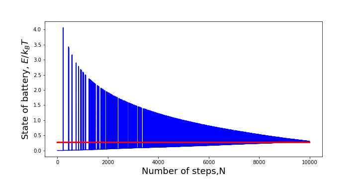
Figure 6: Quasistatic evolution of battery state over a finite number $N$ of bath interactions, under the work-extraction protocol from Skrzypczyk et al.[13] . Red line represents the total nonequilibrium addition to free energy present in the initial input state.

Figure 7: Probability distribution of work extracted, when using the the Skrzypczyk work-extraction protocol with a total of $N=22$ bath interactions. Red line represents the distribution when the protocol—thermodynamically ideal for some mixed state very close to $\ket{0}$—acts on the pure state $\ket{0}$. Blue represent the same protocol’s work distribution when acting on a relatively non-orthogonal pure state $\ket{\psi}$, where fidelity between the two states is $F\bigl{(}\ket{0},\ket{\psi}\bigr{)}=|\braket{0}{\psi}|^{2}=4/5$.

Here we elaborate on the the method of simulations. We considered a string of output with length $n=5000$ produced by the the perturbed-coin process. The possible emissions are $\sigma^{(0)}=\ket{0}\bra{0}$ and $\sigma^{(1)}=\ket{\psi}\bra{\psi}$ where $\ket{\psi}=\sqrt{r}\ket{0}+\sqrt{1-r}\ket{1}$. Here we considered two pure states—this however is not necessary: mixed states can be used too.

For the thermalization, the number of SWAP operations (between system and tailored baths) was chosen to be $N=200$ due to limitation in computational power. One can refer to Fig. 6 to see that as $N\to\infty$ the protocol indeed extracts all the free energy from the system. After the extraction, the change in the battery system is measured and recorded. As mentioned in a previous section, if $N\to\infty$, the work distribution will converge to a set of $\delta$-functions. If $N$ is finite, the probability distribution of the work measured becomes more diffuse, as shown in Fig. 7. The state of knowledge is updated via Bayesian inference, conditioned on the observed work value. This inference step is notably absent from the memoryless approach, where the state of knowledge effectively remains at the initial state of ignorance ${\bm{\upeta}}_{t}={\bm{\uppi}}$.

For the classical protocol, we assume that energetic coherences are inaccessible. In this case, our simulations utilize the Skrzypczyk work-extraction protocol tailored to the decohered state $\rho_{t}^{*}=\xi_{t}^{\text{dec}}$. However, initial decoherence in any other basis, besides $\xi_{t}$’s eigenbasis, would likewise underperform compared to the memory-assisted quantum protocol.

The overcommitment protocol differs from the rest as it tailors the extraction protocol for the state with the highest probability of emission. The probability of emission can be calculated from the state of knowledge ${\bm{\upeta}}_{t}T^{(x)}{\bm{1}}$. The graphs in Panels (c) and (d) of Fig 4 display only positive work-extraction values on the vertical axis; hence most of the data points for overcommitment are not shown owing to its bad performance.

Appendix H Expected work extraction from the four approaches

Here, we derive analytical expressions for the expectation value of work extraction from the various approaches compared in the main text. We derive these expressions for the ($p$, $r$)-parametrized family of perturbed-coin processes of classically correlated quantum states discussed in the main text.

Recall that the quantum states $(\sigma^{(x)})_{x\in\mathcal{X}}$ are the outputs of a Mealy HMM with labeled transition matrices $(T^{(x)})_{x\in\mathcal{X}}$. An element of the labeled transition matrix $T_{s\to s^{\prime}}^{(x)}=\Pr(X_{t}=x,S_{t}=s^{\prime}|S_{t-1}=s)$ gives the joint probability of producing quantum state $\sigma^{(x)}$ and arriving at latent state $s^{\prime}$, given that the HMM begins in state $s$.

For the perturbed-coin example, the HMM’s labeled transition matrices are

$$T^{(0)}=\begin{bmatrix}1-p&0\\ p&0\end{bmatrix}\qquad\text{and }\quad T^{(1)}=\begin{bmatrix}0&p\\ 0&1-p\end{bmatrix}~{}.$$ (54)

The stationary distribution over the latent states is ${\bm{\uppi}}=\left[\frac{1}{2},\frac{1}{2}\right]$ and the two different quantum states created are

$$\sigma^{(0)}=\ket{0}\bra{0}=\begin{bmatrix}1&0\\ 0&0\end{bmatrix}\quad\text{and }\quad\sigma^{(1)}=\ket{\psi}\bra{\psi}=\begin{bmatrix}r&\sqrt{r(1-r)}\\ \sqrt{r(1-r)}&1-r\end{bmatrix}~{}.$$ (55)

For any state of knowledge, ${\bm{\upeta}}_{t}=\left[\frac{1}{2}+\epsilon_{t},\frac{1}{2}-\epsilon_{t}\right]$ parameterized by $\epsilon_{t}\in[-\frac{1}{2},\frac{1}{2}]$, the induced expected state is

$$\xi_{t} =\rho^{(\epsilon_{t})}:=\sum_{x}\begin{bmatrix}\tfrac{1}{2}+\epsilon_{t}&\tfrac{1}{2}-\epsilon_{t}\end{bmatrix}T^{(x)}\mathbf{1}\sigma^{(x)}=\tfrac{1}{2}\begin{bmatrix}1+r+\epsilon_{t}^{\prime}\sqrt{1-r}\,\,&\sqrt{r(1-r)}-\epsilon_{t}^{\prime}\sqrt{r}\\ \sqrt{r(1-r)}-\epsilon_{t}^{\prime}\sqrt{r}\,\,&1-r-\epsilon_{t}^{\prime}\sqrt{1-r}\end{bmatrix}~{},$$ (56)

where $\epsilon^{\prime}:=2\epsilon(1-2p)\sqrt{1-r}\;\propto\epsilon$.

H.1 Memory-assisted quantum processing

In the memory-assisted quantum approach, we utilize work-extraction protocols that are thermodynamically optimized for the expected quantum state

$$\rho_{t}^{*}=\xi_{t}=\rho^{(\epsilon_{t})}~{}.$$ (57)

Recall that the eigenvalues and eigenstates of $\rho_{t}^{*}$ play a prominent role in the work-extraction statistics. We find that the eigenvalues of $\rho^{(\epsilon)}$ are

$$\lambda_{\pm}^{(\rho^{(\epsilon)})}=\tfrac{1}{2}\pm\tfrac{1}{2}\sqrt{r+\epsilon^{\prime 2}}~{},$$ (58)

with corresponding eigenstates

$$\ket{\lambda_{\pm}^{(\rho^{(\epsilon)})}}=2^{-1/2}\Bigl{[}r+\epsilon^{\prime 2}\mp\bigl{(}r+\epsilon^{\prime}\sqrt{1-r}\,\bigr{)}\sqrt{r+\epsilon^{\prime 2}}\,\Bigr{]}^{-1/2}\begin{bmatrix}\sqrt{r(1-r)}-\epsilon^{\prime}\sqrt{r}\\ -r-\epsilon^{\prime}\sqrt{1-r}\pm\sqrt{r+\epsilon^{\prime 2}}\end{bmatrix}~{}.$$ (59)

For all times after $t=0$, the update rule for belief states simplifies to the following

$${\bm{\upeta}}_{t+1}\Bigr{|}_{W_{t+1}=w^{(\pm)}} =\frac{\sum_{x\in\mathcal{X}}\bra{\lambda_{\pm}^{(\xi_{t})}}\sigma^{(x)}\ket{\lambda_{\pm}^{(\xi_{t})}}\,{\bm{\upeta}}_{t}T^{(x)}}{\lambda_{\pm}^{(\xi_{t})}}~{},$$ (60)

which can be expressed explicitly in terms of $p$, $r$, and $\epsilon_{t}$.

When $\epsilon_{t}=0$, we find that ${\bm{\upeta}}_{t+1}=\Bigl{[}\frac{1}{2},\frac{1}{2}\Bigr{]}={\bm{\uppi}}$. I.e., the stationary distribution is a fixed point for this dynamic over belief states. Because of this, we break the initial symmetry by setting $\epsilon$ to a small non-zero value to obtain useful knowledge. In other words, for the very first work-extraction protocol, we choose some $\rho_{0}^{*}\neq\xi_{0}$ to avoid an unstable fixed point of the update rule. However, for all subsequent time steps, we choose $\rho_{t}^{*}=\xi_{t}$.

For the perturbed coin, the metadynamic of the belief state in the long run will yield two different results, depending on which regime the system is in, “memory-apathetic regime” or “memory-advantageous regime”. The reason for this separation comes from the shape of their update function. For the memory-apathetic region, the update function has gradient less than unity, making $\epsilon=0$ an attractor. For the memory-advantageous region, the gradient of the update function exceeds unity, therefore making $\epsilon=0$ a repellor, at the same time two other points become part of a new attractor.

In the long run, transient belief states die out, leaving only the steady-state dynamics among the recurrent states of knowledge; any initial distribution over belief states generically converges to the stationary measure $\bm{\pi}_{\mathcal{K}}$. Hence the steady-state rate of work extraction is given by

$$\lim_{t\to\infty}\langle{W_{t}}\rangle=k_{\text{B}}T\langle\text{D}[\xi_{t}\|\gamma]\rangle_{\Pr(K_{t})=\bm{\pi}_{\mathcal{K}}}~{},$$ (61)

The expected extracted work for the memory-apathetic region coincide with that of memoryless extraction and is given by

$$\left\langle W^{\text{apathetic}}\right\rangle=k_{\text{B}}T\text{D}[\xi_{0}\|\gamma]=\left\langle W^{\text{memoryless}}\right\rangle~{}.$$ (62)

On the other hand, in the regime where memory enhances the performance of the protocol, the stationary distribution over the two recurrent belief states ${\bm{\upeta}}$ and ${\bm{\upeta}}^{\prime}$, with corresponding expected quantum states $\xi$ and $\xi^{\prime}$, is

$$\bm{\pi}_{\mathcal{K}}=\frac{1}{\lambda^{(\xi)}_{+}+\lambda^{(\xi^{\prime})}_{+}}[\lambda^{(\xi^{\prime})}_{+},\lambda^{(\xi)}_{+}]~{}.$$ (63)

Hence, the work extraction rate is given by

$$\left\langle W^{\text{advantage}}\right\rangle=\frac{k_{\text{B}}T}{\lambda^{(\xi)}_{+}+\lambda^{(\xi^{\prime})}_{+}}\Bigl{(}\lambda^{(\xi^{\prime})}_{+}\text{D}[\xi\|\gamma]+\lambda^{(\xi)}_{+}\text{D}[\xi^{\prime}\|\gamma]\Bigr{)}~{}.$$ (64)

H.2 Classical approach

The derivation for the memory-assisted classical approach is similar to that of the memory-assisted quantum approach illustrated above. However rather than operating on the induced expected state $\xi_{t}$, the classical approach uses work-extraction protocols that are thermodynamically optimized for the decohered state

$$\rho_{t}^{*}=\xi_{t}^{\text{dec}}=\frac{1}{2}\begin{bmatrix}1+r+\epsilon_{t}^{\prime}\sqrt{1-r}\,\,&0\\ 0\,\,&1-r-\epsilon_{t}^{\prime}\sqrt{1-r}\end{bmatrix}~{}.$$ (65)

The eigenstates of $\rho_{t}^{*}$ are thus $\ket{0}$ and $\ket{1}$, independent of time in this case. In the classical approach, ${\bm{\uppi}}$ is no longer a fixed point of the belief-state update maps. The transition probabilities between belief states are now given by

$$\lambda_{\pm}^{(\xi_{t}^{\text{dec}})}=\tfrac{1}{2}\Bigl{[}1\pm\bigl{(}r+\epsilon_{t}^{\prime}\sqrt{1-r}\,\bigr{)}\Bigr{]}~{}.$$ (66)

The metadynamic of belief in the classical case behaves as a reset processes. Unlike the quantum case with only two recurrent belief states, the classical protocol induces an infinite set of recurrent belief states. To construct a finite-state autonomous engine, we could choose to truncate those states within some small $\delta$ distance from another recurrent state, or truncate belief states with negligible probability, with vanishing work-extraction penalty.

We find that the work-extraction rate can again be computed by averaging the relative entropy—now between the decohered expected state and thermal state—over all recurrent states of knowledge:

$$\langle W_{t}^{\text{classical}}\rangle=k_{\text{B}}T\langle\text{D}[\xi_{t}^{\text{dec}}\|\gamma]\rangle_{\Pr(K_{t}^{\text{classical}})}~{}.$$ (67)

H.3 Overcommitment to the most likely outcome

The “overcommitment” approach used for comparison in the main text bets exclusively on the most likely outcome in $\{\sigma^{(x)}\}_{x}$.

The expected thermodynamic cost of misaligned expectations during work extraction can be quantified exactly via the relative entropy $\text{D}[\rho_{0}\|\alpha_{0}]$ between the actual input $\rho_{0}$ and the anticipated input $\alpha_{0}$ that the protocol is optimal for, if we assume that the final state is independent of the initial state [31, 32]. Hence, if we design the protocol for a pure state, but operate on a mixed state, we will encounter divergent thermodynamic penalties.

Accordingly, we can observe divergent thermodynamic costs when we design the Skrzypczyk work extraction protocol to be optimal for operation on a pure state.

Using the Skrzypczyk protocol (with $N$ relaxation steps) to extract work from the pure state bet upon, we see that the first bath state swapped with the system for energy extraction is not exactly pure, but rather satisfies $\gamma_{\text{B}}=\Bigl{(}1-\frac{e^{-\beta E_{0}}}{N(e^{-\beta E_{0}}+e^{-\beta E_{1}})}\Bigr{)}\ket{0}\bra{0}+\frac{e^{-\beta E_{1}}}{N(e^{-\beta E_{0}}+e^{-\beta E_{1}})}\ket{1}\bra{1}$. (Recall that $H$ is the Hamiltonian for the system, not of the bath.) Any purity of the actual input beyond this initial bath purity is wasted. The input state leading to minimal entropy production under this protocol is thus a unitary rotation of $\gamma_{\text{B}}$.

Thus, for this use case of the Skrzypczyk protocol, the minimally dissipative state $\alpha_{0}$ becomes pure as $N\to\infty$. As $N\to\infty$, we observe the battery’s final expected energy diverging (but only logarithmically in $N$) to negative infinity, when this protocol acts on any other state. I.e., $\langle W\rangle\sim-k_{\text{B}}T\ln N$.

More specifically, we can leverage Eqs. (5) and (6) to calculate the expected value of work for the overcommitment approach. We find that

$$\Pr(W=w^{(-)}|\sigma^{(\text{argmin}_{x}{\bm{\upeta}}_{t}T^{(x)}\mathbf{1})})=|\braket{1}{\psi}|^{2}=1-r~{}.$$ (68)

With $\lambda_{-}=\frac{e^{-\beta E_{1}}}{N(e^{-\beta E_{0}}+e^{-\beta E_{1}})}$, $w^{(-)}\sim-k_{\text{B}}T\ln N$, and $\text{min}_{x}{\bm{\upeta}}_{t}T^{(x)}\mathbf{1}\sim\text{min}(p,1-p)$ when ${\bm{\upeta}}_{t}$ is close to either latent state, we anticipate that the overcommited work penalty diverges as $-k_{\text{B}}T(1-r)\min(p,1-p)\ln N$, as observed.

Interestingly, for a finite number of bath interactions, some work can be extracted on average within certain regimes. But other regions of parameter space would yield very negative work-extraction averages.

Unlike the other approaches, the expectation value of work in the overcommitment approach cannot be written as a relative entropy. Hence, whereas the other approaches were guaranteed to have non-negative work extraction on average, the overcommitment approach enjoys no such guarantee of non-negativity. Indeed in the limit of many bath interactions, the overcommitment approach leads to infinitely negative work extraction.

Appendix I Quantum Information Processing Second Law

Here, we derive the Quantum Information Processing Second Law (QIPSL), which generalizes the classical IPSL of Refs. [8, 43, 33, 44, 45, 35, 46] in several directions.

We consider the fundamental thermodynamic limits of a memoryful physical transducer that consumes one physical pattern and produces another. Both the input and output are assumed to be stationary quantum stochastic processes. Although much of the previous information-engines literature restricts itself to the energy-degenerate case (such that a ‘0’ and ‘1’ have the same energy), here we generalize to allow the Hamiltonian for each subsystem to be either degenerate or non-degenerate.

Denote the joint state of a $d_{\text{\text{M}}}$-dimensional memory and the length-$L$ pattern as $\rho_{t}^{(\text{M},1:L)}$, with corresponding reduced states of the memory $\rho_{t}^{(\text{M})}$ and of the pattern $\rho_{t}^{(1:L)}$. If we denote $W_{\tau}^{\text{ext}}=\sum_{t=1}^{\tau}W_{t}$ as the net work extracted up to time $\tau$, then the second law of thermodynamics tells us that the change in nonequilibrium free energy $\mathcal{F}_{t}^{(\text{M},1:L)}$ upper bounds the expectation value of extracted work when the environment is at the fixed temperature $T$ [10]. We assume cyclic transformations where the joint Hamiltonian at time $\tau$ is the same as the the joint Hamiltonian at time $0$—although it may be modulated during the protocol to enable the work extraction. The equilibrium state $\bm{\gamma}$ for the joint pattern and memory is thus the same at times $0$ and $\tau$. For this reason, there is no net change in equilibrium free energy. Accordingly, the only change in nonequilibrium free energy is due to the change in the nonequilbrium addition to free energy—the quantum relative entropy between the actual state and the equilibrium state:

$$\braket{W_{\tau}^{\text{ext}}} \leq\mathcal{F}_{0}^{(\text{M},1:L)}-\mathcal{F}_{\tau}^{(\text{M},1:L)}$$

$$=k_{\text{B}}T\text{D}[\rho_{0}^{(\text{M},1:L)}\|\bm{\gamma}]-k_{\text{B}}T\text{D}[\rho_{\tau}^{(\text{M},1:L)}\|\bm{\gamma}]~{}.$$ (69)

We now make several assumptions relevant to energetically-efficient memoryful pattern manipulation:

1. We will assume that the memory is fully energetically degenerate so that unitary memory updates do not cost energy. Then $\bm{\gamma}=(I/d_{\text{M}})\otimes\gamma^{\otimes L}$ describes the equilibrium state of the joint supersystem.

2. Since the memory is always initialized as a particular memory state $\rho_{0}^{(\text{M})}$, the memory and pattern are initially uncorrelated: $\rho_{0}^{(\text{M},1:L)}=\rho_{0}^{(\text{M})}\otimes\rho_{0}^{(1:L)}$.

3. Through the sequence of deterministic updates, and equal (possibly zero) internal entropy of each memory state, the entropy of the memory is unchanging.

Altogether, these features imply that the extractable work is upper bounded by

$$\frac{\braket{W_{\tau}^{\text{ext}}}}{k_{\text{B}}T} \leq\text{D}[\rho_{0}^{(1:L)}\|\gamma^{\otimes L}]-\text{D}[\rho_{\tau}^{(1:L)}\|\gamma^{\otimes L}]-\text{I}_{\tau}$$ (70)

$$=-\text{I}_{\tau}+\Delta\text{S}(\rho_{t}^{(1:L)})+\Delta\sum_{\ell=1}^{L}\mathrm{Tr}(\rho_{t}^{(\ell)}\ln\gamma)~{},$$ (71)

where $\text{I}_{t}=\text{D}[\rho_{t}^{(\text{M},1:L)}\|\rho_{t}^{(\text{M})}\otimes\rho_{t}^{(1:L)}]$ is the mutual information that has built up between the memory and the quantum pattern. The operator $\Delta$ evaluates the difference of each function from time $t=0$ to time $t=\tau$, such that $\Delta f_{t}\equiv f_{\tau}-f_{0}$ for any function $f$ of $t$.

The classical IPSL, and the quantum generalization we derive, address the scenario where a physical machine scans unidirectionally along the pattern. After $\tau$ time-steps, the first $\tau$ subsystems of the pattern have interacted with the machine, while the other subsystems remain unaltered: $\rho_{\tau}^{(\tau+1:L)}=\rho_{0}^{(\tau+1:L)}$.

More specifically, the IPSL assumes that both the input tape and output tape are stationary stochastic processes, such that all marginal distributions of each (input or output) is shift invariant within the domain of the existing pattern. We likewise consider the case that both input and output processes have a well-defined von Neumann entropy rate $s_{\text{vN}}$ and $s_{\text{vN}}^{\prime}$ respectively. Each also has a myopic entropy rate $s_{\ell}=\text{S}(\rho_{0}^{(1:\ell)})-\text{S}(\rho_{0}^{(1:\ell-1)})$ and $s_{\ell}^{\prime}=\text{S}(\rho_{\tau}^{(1:\ell)})-\text{S}(\rho_{\tau}^{(1:\ell-1)})$ for $\ell\leq\tau$, with $s_{1}=\text{S}(\rho_{0}^{(1)})$ and $s_{1}^{\prime}=\text{S}(\rho_{\tau}^{(1)})$. The myopic entropy rate describes the convergence to irreducible randomness in pattern extension, as progressively more subsystems are prefixed. Relatedly, the myopic excess entropy for the input process is $\mathcal{E}_{\ell}=\sum_{n=1}^{\ell}(s_{n}-s_{\text{vN}})$, with a similar relation for the primed output process. Asymptotically, the excess entropy describes the quantum mutual information between the past and future of a bi-infinite process: $\lim_{\ell\to\infty}\mathcal{E}_{\ell}=\mathcal{E}=\lim_{\ell\to\infty}\text{I}(\rho_{0}^{(1:\ell)};\rho_{0}^{(\ell+1:2\ell)})$.

With these definitions and assumptions in place, we can now expand Eq. (71) to derive the QIPSL:

$$\frac{\braket{W_{\tau}^{\text{ext}}}}{k_{\text{B}}T} \leq-\text{I}_{\tau}+\Delta\text{S}(\rho_{t}^{(1:L)})+\Delta\sum_{\ell=1}^{L}\mathrm{Tr}(\rho_{t}^{(\ell)}\ln\gamma)$$

$$=-\text{I}_{\tau}+\Delta\text{S}(\rho_{t}^{(1:L)})+\Delta\sum_{\ell=1}^{\tau}\mathrm{Tr}(\rho_{t}^{(\ell)}\ln\gamma)$$ (72)

$$=-\text{I}_{\tau}+\Delta\text{S}(\rho_{t}^{(1:L)})+\tau\Delta\mathrm{Tr}(\rho_{t}^{(1)}\ln\gamma)~{}.$$ (73)

Now, note that

$$\Delta\text{S}(\rho_{t}^{(1:L)}) =\Delta\text{S}(\rho_{t}^{(1:\tau)})+\underbrace{\Delta\text{S}(\rho_{t}^{(\tau+1:L)})}_{=0}-\Delta\text{I}(\rho_{t}^{(1:\tau)};\rho_{t}^{(\tau+1:L)})$$ (74)

$$=-\text{I}(\rho_{\tau}^{(1:\tau)};\underbrace{\rho_{\tau}^{(\tau+1:L)}}_{=\rho_{0}^{(\tau+1:L)}})+\underbrace{\Delta\text{S}(\rho_{t}^{(1:\tau)})}_{\tau(s_{\text{vN}}^{\prime}-s_{\text{vN}})+\mathcal{E}_{\tau}^{\prime}-\mathcal{E}_{\tau}}+\underbrace{\text{S}(\rho_{0}^{(1:\tau)})+\text{S}(\rho_{0}^{(\tau+1:L)})-\text{S}(\rho_{0}^{(1:L)})}_{\mathcal{E}_{\tau}+\mathcal{E}_{L-\tau}-\mathcal{E}_{L}}$$ (75)

$$=-\text{I}(\rho_{\tau}^{(1:\tau)};\rho_{0}^{(\tau+1:L)})+\tau(s_{\text{vN}}^{\prime}-s_{\text{vN}})+\mathcal{E}_{\tau}^{\prime}-(\mathcal{E}_{L}-\mathcal{E}_{L-\tau})~{}.$$ (76)

Thus, plugging this back in to Eq. (73), we arrive at the Quantum Information Processing Second Law (QIPSL):

$$\frac{\braket{W_{\tau}^{\text{ext}}}}{k_{\text{B}}T} \leq-\text{I}_{\tau}-\text{I}(\rho_{\tau}^{(1:\tau)};\rho_{0}^{(\tau+1:L)})+\tau(s_{\text{vN}}^{\prime}-s_{\text{vN}})+\mathcal{E}_{\tau}^{\prime}-(\mathcal{E}_{L}-\mathcal{E}_{L-\tau})+\tau\Delta\mathrm{Tr}(\rho_{t}^{(1)}\ln\gamma)~{}.$$ (77)

Under typical assumptions like finite memory, the time-extensive rate of work extraction during sequential quantum pattern manipulation is thus upper bounded by $s_{\text{vN}}^{\prime}-s_{\text{vN}}+\Delta\mathrm{Tr}(\rho_{t}^{(1)}\ln\gamma)$, in units of $k_{\text{B}}T$:

$$\lim_{\tau\to\infty}\frac{\braket{W_{\tau}^{\text{ext}}}}{\tau k_{\text{B}}T} \leq s_{\text{vN}}^{\prime}-s_{\text{vN}}+\Delta\mathrm{Tr}(\rho_{t}^{(1)}\ln\gamma)~{}.$$ (78)

Furthermore, if the Hamiltonian of each subsystem is fully degenerate, then $\Delta\mathrm{Tr}(\rho_{t}^{(1)}\ln\gamma)=0$, which would yield $\lim_{\tau\to\infty}\frac{\braket{W_{\tau}^{\text{ext}}}}{\tau k_{\text{B}}T}\leq s_{\text{vN}}^{\prime}-s_{\text{vN}}$—analogous to the typical statement of the classical IPSL, but with von Neumann entropy density in place of the classical entropy density.

To be thermodynamically efficient, it is known that the classical machine needs to be predictive or retrodictive in the case that it is consuming or generating a process, respectively [33, 16, 34, 35]. From Eq. (77), we now see that an analogous result remains true in the more general quantum case.

It is worth reflecting on the behavior of the contributions to Eq. (77). Notably, $\mathcal{E}_{L}-\mathcal{E}_{L-\tau}\geq 0$, with $\mathcal{E}_{L}-\mathcal{E}_{L-\tau}\approx 0$ when $L-\tau\gg 0$, and $\mathcal{E}_{L}-\mathcal{E}_{L-\tau}\to\mathcal{E}_{L}\approx\mathcal{E}$ as $\tau\to L$. Meanwhile, the myopic excess entropy for the output process is a non-decreasing function of $\tau$ that approaches the past–future quantum mutual information of the output process $\mathcal{E}_{\tau}^{\prime}\approx\mathcal{E}^{\prime}$ whenever $\tau\gg 0$.

I.1 Implications for work extraction

What are the implications for work extraction? We note that after $t$ time-steps of work extraction from a quantum pattern, the first $t$ subsystems of the pattern have been brought to their equilibrium states, while the other subsystems remain unaltered: $\rho_{t}^{(1:L)}=\gamma^{\otimes t}\otimes\rho_{0}^{(t+1:L)}$. Hence $\text{I}(\rho_{\tau}^{(1:\tau)};\rho_{0}^{(\tau+1:L)})=0$, and $\text{I}_{\tau}=\text{D}[\rho_{\tau}^{(\text{M},\tau+1:L)}\|\rho_{\tau}^{(\text{M})}\otimes\rho_{\tau}^{(\tau+1:L)}]$ with $\text{I}_{\tau}\to 0$ as $\tau\to L$. Since the output process produces an IID sequence of Gibbs states, we have $\mathcal{E}_{t}^{\prime}=0$, while the entropy rate of the output equals the entropy of the Gibbs state $s_{\text{vN}}^{\prime}=\text{S}(\gamma)$.

Eq. (77) thus simplifies in this setting to become

$$\frac{\braket{W_{\tau}^{\text{ext}}}}{k_{\text{B}}T} \leq-\text{I}_{\tau}-\tau s_{\text{vN}}-(\mathcal{E}_{L}-\mathcal{E}_{L-\tau})-\tau\mathrm{Tr}(\rho_{0}^{(\ell)}\ln\gamma)$$ (79)

$$=-\text{I}_{\tau}+\tau[\text{S}(\rho_{0}^{(\ell)})-s_{\text{vN}}]-(\mathcal{E}_{L}-\mathcal{E}_{L-\tau})+\tau\text{D}[\rho_{0}^{(\ell)}\|\gamma]~{},$$ (80)

where the choice of $\ell\in\{1,2,\dots,L\}$ is arbitrary since we assume a stationary quantum pattern.

For a long pattern, the asymptotic work-extraction rate is $\braket{W_{t}}=\lim_{\tau\to\infty}\frac{W_{\tau}^{\text{ext}}}{\tau}$. When the work-extraction device has a finite memory, so that $\lim_{\tau\to\infty}\frac{\text{I}_{\tau}}{\tau}=0$, we thus find that the steady-state work-extraction rate is upper bounded by

$$\frac{\braket{W_{t}}}{k_{\text{B}}T}\,\leq\,\text{S}(\rho_{0}^{(\ell)})-s_{\text{vN}}+\text{D}[\rho_{0}^{(\ell)}\|\gamma]\,\eqqcolon\,\frac{w^{\text{ideal}}}{k_{\text{B}}T}~{}.$$ (81)

When there is still plenty of input pattern remaining—i.e., when $L-\tau$ is sufficiently large such that $\mathcal{E}_{L}-\mathcal{E}_{L-\tau}\approx 0$—we find $\braket{W_{\tau}^{\text{ext}}}\leq\tau w^{\text{ideal}}-k_{\text{B}}T\,\text{I}_{\tau}$. On the other hand, when the entire pattern has been consumed, $\text{I}_{L}=0$ yet $\mathcal{E}_{L}-\mathcal{E}_{0}=\mathcal{E}_{L}\approx\mathcal{E}$ for sufficiently large $L$, leading to

$$\braket{W_{L}^{\text{ext}}}\leq Lw^{\text{ideal}}-k_{\text{B}}T\mathcal{E}~{}.$$ (82)

Appendix J Non-Markovian generators

Unlike the classical case, the classical control symbols $X_{t}$ are hidden from direct observation when the process emits non-orthogonal quantum states. The latent-state generators may thus be referred to as ‘doubly-hidden Markov models’. Accordingly, even if the intermediary $X_{t}$ process is Markovian, this would not directly imply a meaningful sense of quantum Markovianity of the outputs. Nevertheless, there is some sense in which processes with non-Markovian control outputs $X_{t}$ have more deeply hidden structure.

To benchmark the performance of the memory-assisted protocol on a process with higher Markov order of the control symbols $X_{t}$, the 2-1 golden-mean process was chosen for comparison. The time-averaged density matrix of the memoryless approach for both models is kept the same, $\xi_{0}=\frac{1}{2}(\sigma^{(0)}+\sigma^{(1)})$. The comparison is shown in Fig. 8, where we see that more work is extracted from the non-Markovian generator. This example suggests that memory can become even more important for enabling work extraction from non-Markovian generators of quantum processes, since the extractable structure can be more deeply hidden.

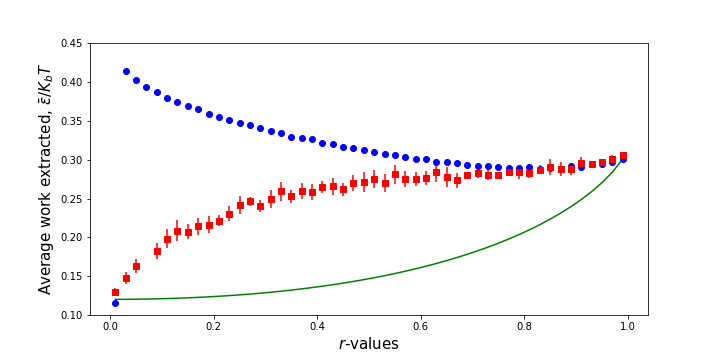
Figure 8: Comparison of average work extracted between 2-1 golden-mean and perturbed-coin processes, varying the nonorthogonality parameter $r$. Blue and red dots represent the memory-assisted quantum approach on golden mean and perturbed coin respectively; Green line represents the memoryless approach.

References

- [1] Daniel V Schroeder. “An introduction to thermal physics”. American Association of Physics Teachers. (1999). doi: 10.1119/1.19116.
- [2] Stephen J Blundell and Katherine M Blundell. “Concepts in thermal physics”. Oup Oxford. (2009). doi: 10.1093/acprof:oso/9780199562091.001.0001.
- [3] James Sethna. “Statistical mechanics: entropy, order parameters, and complexity”. Volume 14. Oxford University Press, USA. (2021). doi: 10.1093/oso/9780198865247.001.0001.
- [4] Herbert B Callen. “Thermodynamics and an introduction to thermostatistics”. John wiley & sons. (1991). doi: 10.1119/1.14986.
- [5] Leo Szilard. “On the decrease of entropy in a thermodynamic system by the intervention of intelligent beings”. Behavioral Science 9, 301–310 (1964). doi: 10.1002/bs.3830090402.
- [6] Rolf Landauer. “Irreversibility and heat generation in the computing process”. IBM journal of research and development 5, 183–191 (1961). doi: 10.1147/rd.53.0183.
- [7] Charles H Bennett. “The thermodynamics of computation—a review”. International Journal of Theoretical Physics 21, 905–940 (1982). doi: 10.1007/BF02084158.
- [8] Dibyendu Mandal and Christopher Jarzynski. “Work and information processing in a solvable model of Maxwell’s demon”. Proceedings of the National Academy of Sciences 109, 11641–11645 (2012). doi: 10.1073/pnas.1204263109.
- [9] Dibyendu Mandal, HT Quan, and Christopher Jarzynski. “Maxwell’s refrigerator: an exactly solvable model”. Physical review letters 111, 030602 (2013). doi: 10.1103/PhysRevLett.111.030602.
- [10] Juan MR Parrondo, Jordan M Horowitz, and Takahiro Sagawa. “Thermodynamics of information”. Nature physics 11, 131–139 (2015). doi: 10.1038/nphys3230.
- [11] John Goold, Marcus Huber, Arnau Riera, Lídia Del Rio, and Paul Skrzypczyk. “The role of quantum information in thermodynamics—a topical review”. Journal of Physics A: Mathematical and Theoretical 49, 143001 (2016). doi: 10.1088/1751-8113/49/14/143001.
- [12] Felix Binder, Luis A Correa, Christian Gogolin, Janet Anders, and Gerardo Adesso. “Thermodynamics in the quantum regime”. Fundamental Theories of Physics 195, 1–2 (2018). doi: 10.1007/978-3-319-99046-0.
- [13] Paul Skrzypczyk, Anthony J Short, and Sandu Popescu. “Work extraction and thermodynamics for individual quantum systems”. Nature communications5 (2014). doi: 10.1038/ncomms5185.
- [14] Johan Åberg. “Catalytic coherence”. Physical review letters 113, 150402 (2014). doi: 10.1103/PhysRevLett.113.150402.
- [15] Kamil Korzekwa, Matteo Lostaglio, Jonathan Oppenheim, and David Jennings. “The extraction of work from quantum coherence”. New Journal of Physics 18, 023045 (2016). doi: 10.1088/1367-2630/18/2/023045.
- [16] Andrew JP Garner, Jayne Thompson, Vlatko Vedral, and Mile Gu. “Thermodynamics of complexity and pattern manipulation”. Physical Review E 95, 042140 (2017). doi: 10.1103/PhysRevE.95.042140.
- [17] Matteo Lostaglio. “Thermodynamic laws for populations and quantum coherence: A self-contained introduction to the resource theory approach to thermodynamics” (2018). doi: 10.48550/arXiv.1807.11549.
- [18] James P Crutchfield and Karl Young. “Inferring statistical complexity”. Physical review letters 63, 105 (1989). doi: 10.1103/PhysRevLett.63.105.
- [19] Cosma Rohilla Shalizi and James P Crutchfield. “Computational mechanics: Pattern and prediction, structure and simplicity”. Journal of statistical physics 104, 817–879 (2001). doi: 10.1023/A:1010388907793.
- [20] James P Crutchfield. “Between order and chaos”. Nature Physics 8, 17–24 (2012). doi: 10.1038/nphys2190.
- [21] Alexander B. Boyd, Dibyendu Mandal, and James P. Crutchfield. “Correlation-powered information engines and the thermodynamics of self-correction”. Phys. Rev. E 95, 012152 (2017). doi: 10.1103/PhysRevE.95.012152.
- [22] Michael A Nielsen and Isaac Chuang. “Quantum computation and quantum information”. Cambridge University Press. (2011). doi: 10.1017/CBO9780511976667.
- [23] Philipp Strasberg, Gernot Schaller, Tobias Brandes, and Massimiliano Esposito. “Quantum and information thermodynamics: A unifying framework based on repeated interactions”. Phys. Rev. X 7, 021003 (2017). doi: 10.1103/PhysRevX.7.021003.
- [24] Kavan Modi, Tomasz Paterek, Wonmin Son, Vlatko Vedral, and Mark Williamson. “Unified view of quantum and classical correlations”. Phys. Rev. Lett. 104, 080501 (2010). doi: 10.1103/PhysRevLett.104.080501.
- [25] Ariadna E Venegas-Li, Alexandra M Jurgens, and James P Crutchfield. “Measurement-induced randomness and structure in controlled qubit processes”. Physical Review E 102, 040102 (2020). doi: 10.1103/PhysRevE.102.040102.
- [26] James P Crutchfield. “The calculi of emergence: computation, dynamics and induction”. Physica D: Nonlinear Phenomena 75, 11–54 (1994). doi: 10.1016/0167-2789(94)90273-9.
- [27] Christopher J Ellison, John R Mahoney, and James P Crutchfield. “Prediction, retrodiction, and the amount of information stored in the present”. Journal of Statistical Physics 136, 1005–1034 (2009). doi: 10.1007/s10955-009-9808-z.
- [28] Sarah E Marzen and James P Crutchfield. “Nearly maximally predictive features and their dimensions”. Physical Review E 95, 051301 (2017). doi: 10.1103/PhysRevE.95.051301.
- [29] Paul M Riechers and James P Crutchfield. “Spectral simplicity of apparent complexity. I. The nondiagonalizable metadynamics of prediction”. Chaos: An Interdisciplinary Journal of Nonlinear Science 28, 033115 (2018). doi: 10.1063/1.4985199.
- [30] Alexandra M Jurgens and James P Crutchfield. “Shannon entropy rate of hidden Markov processes”. Journal of Statistical Physics 183, 1–18 (2021). doi: 10.1007/s10955-021-02769-3.
- [31] Paul M Riechers and Mile Gu. “Initial-state dependence of thermodynamic dissipation for any quantum process”. Physical Review E 103, 042145 (2021). doi: 10.1103/PhysRevE.103.042145.
- [32] Paul M Riechers and Mile Gu. “Impossibility of achieving Landauer’s bound for almost every quantum state”. Phys. Rev. A 104, 012214 (2021). doi: 10.1103/PhysRevA.104.012214.
- [33] Alexander B Boyd, Dibyendu Mandal, Paul M Riechers, and James P Crutchfield. “Transient dissipation and structural costs of physical information transduction”. Physical review letters 118, 220602 (2017). doi: 10.1103/PhysRevLett.118.220602.
- [34] Alexander B Boyd, Dibyendu Mandal, and James P Crutchfield. “Thermodynamics of modularity: Structural costs beyond the Landauer bound”. Physical Review X 8, 031036 (2018). doi: 10.1103/PhysRevX.8.031036.
- [35] Andrew JP Garner. “The fundamental thermodynamic bounds on finite models”. Chaos: An Interdisciplinary Journal of Nonlinear Science 31, 063131 (2021). doi: 10.1063/5.0044741.
- [36] Yelena Guryanova, Nicolai Friis, and Marcus Huber. “Ideal Projective Measurements Have Infinite Resource Costs”. Quantum 4, 222 (2020). doi: 10.22331/q-2020-01-13-222.
- [37] Cyril Elouard, David Herrera-Martí, Benjamin Huard, and Alexia Auffeves. “Extracting work from quantum measurement in Maxwell’s demon engines”. Physical Review Letters 118, 260603 (2017). doi: 10.1103/PhysRevLett.118.260603.
- [38] Patryk Lipka-Bartosik, Paweł Mazurek, and Michał Horodecki. “Second law of thermodynamics for batteries with vacuum state”. Quantum 5, 408 (2021). doi: 10.22331/Q-2021-03-10-408.
- [39] F. L. Curzon and B. Ahlborn. “Efficiency of a Carnot engine at maximum power output”. American Journal of Physics 43, 22–24 (1975). doi: 10.1119/1.10023. arXiv:https://pubs.aip.org/aapt/ajp/article-pdf/43/1/22/12091578/22_1_online.pdf.
- [40] John P. S. Peterson, Tiago B. Batalhão, Marcela Herrera, Alexandre M. Souza, Roberto S. Sarthour, Ivan S. Oliveira, and Roberto M. Serra. “Experimental characterization of a spin quantum heat engine”. Phys. Rev. Lett. 123, 240601 (2019). doi: 10.1103/PhysRevLett.123.240601.
- [41] Tan Van Vu and Keiji Saito. “Finite-time quantum Landauer principle and quantum coherence”. Phys. Rev. Lett. 128, 010602 (2022). doi: 10.1103/PhysRevLett.128.010602.
- [42] Philip Taranto, Faraj Bakhshinezhad, Andreas Bluhm, Ralph Silva, Nicolai Friis, Maximilian P.E. Lock, Giuseppe Vitagliano, Felix C. Binder, Tiago Debarba, Emanuel Schwarzhans, Fabien Clivaz, and Marcus Huber. “Landauer versus Nernst: What is the true cost of cooling a quantum system?”. PRX Quantum 4, 010332 (2023). doi: 10.1103/PRXQuantum.4.010332.
- [43] Alexander B Boyd, Dibyendu Mandal, and James P Crutchfield. “Identifying functional thermodynamics in autonomous Maxwellian ratchets”. New Journal of Physics 18, 023049 (2016). doi: 10.1088/1367-2630/18/2/023049.
- [44] Elan Stopnitzky, Susanne Still, Thomas E Ouldridge, and Lee Altenberg. “Physical limitations of work extraction from temporal correlations”. Physical Review E 99, 042115 (2019). doi: 10.1103/PhysRevE.99.042115.
- [45] Alexandra M Jurgens and James P Crutchfield. “Functional thermodynamics of Maxwellian ratchets: Constructing and deconstructing patterns, randomizing and derandomizing behaviors”. Physical Review Research 2, 033334 (2020). doi: 10.1103/PhysRevResearch.2.033334.
- [46] Lianjie He, Andri Pradana, Jian Wei Cheong, and Lock Yue Chew. “Information processing second law for an information ratchet with finite tape”. Physical Review E 105, 054131 (2022). doi: 10.1103/PhysRevE.105.054131.