Q-field from a 4D-brane: Cosmological constant cancellation and Minkowski attractor

Abstract

A 4D-brane realization of $q$-theory has been proposed a few years ago. The present paper studies the corresponding late-time cosmology and establishes the dynamic cancellation of an initial cosmological constant and an attractor behavior towards Minkowski spacetime.

I Introduction

The cosmological constant problem is perhaps the most important problem of modern physics Weinberg1989 . A condensed-matter-inspired approach has been proposed and goes under the name of $q$-theory KlinkhamerVolovik2008a ; KlinkhamerVolovik2008b ; KlinkhamerVolovik2010 . A particular realization of $q$-theory takes its cue from the physics of a freely suspended two-dimensional material film KatsLebedev2015 and uses a generalization to four-dimensional “films” or 4D-branes KlinkhamerVolovik-JETPL-2016-4Dbrane .

This 4D-brane realization of $q$-theory has a dimensionless chemical potential $\mu$ (details will be given shortly) and may be of relevance to a recent suggestion to replace the big bang by a quantum phase transition KlinkhamerVolovik2022-BBasTopQPT .

The goal of the present paper is to discuss the corresponding late-time cosmology, where the asymptotic vacuum energy density may or may not vanish. In particular, we would like to establish a possible attractor behavior towards Minkowski spacetime with a vanishing vacuum energy density. Throughout, we use natural units with $\hbar=1$ and $c=1$.

II Action and field equations

The following 4D-brane action has been proposed in Ref. KlinkhamerVolovik-JETPL-2016-4Dbrane :

$$S = -\int d^{4}x\,\sqrt{-g}\,\left[\frac{R}{16\pi G_{N}}+\epsilon\left(\frac{n}{\sqrt{-g}}\right)+\mathcal{L}^{M}[\psi]\right]+\mu\int\,d^{4}x\;n\,,$$ (1)

with a Lorentzian signature ($-,\,+,\,+,\,+$) of the metric $g_{\alpha\beta}$, so that its determinant $g\equiv\det(g_{\alpha\beta})$ is negative. In (1), the term $\mathcal{L}^{M}(\psi)$ is the matter Lagrange density for a generic matter field $\psi$ and the potential $\epsilon(x)$ is an essentially arbitrary function of $x$ (the stability of the equilibrium state gives some conditions on the potential KlinkhamerVolovik2008a ). The crucial new ingredient of the above action is $n$ as the 4D analog of the particle density of a 2D membrane. This 4D density $n$ may refer to “spacetime atoms,” with the corresponding nonzero chemical potential $\mu$ (further discussion will be given in Sec. IV).

At this moment, it may be helpful to explain the terminology “spacetime atoms.” The physics of the freely suspended two-dimensional material film has been reviewed in the first two paragraphs of Sec. 3 in Ref. KlinkhamerVolovik-JETPL-2016-4Dbrane , with mention of the original reference KatsLebedev2015 . The film there is made out of atoms, whose basic structure is known to be described by the Schrödinger equation. The Hamiltonian of this two-dimensional material film has been generalized to a four-dimensional action and, for this reason, we can perhaps speak of a system describing “spacetime atoms,” whose structure is, of course, completely unknown at the present moment. What matters, for the following, is the structure of the action (1) with an unknown (conserved) quantity $n$ having mass dimension 4.

The resulting $n$-field equation from (1) reads

$$\frac{d\epsilon}{dq} = \mu\,,$$ (2a)

$$q \equiv \frac{n}{\sqrt{-g}}\,.$$ (2b)

Here, we have identified a scalar $q$-field with mass dimension 4, so that $\mu$ has mass dimension 0 and this $q$-field realization may be relevant to the big-bang discussion of Ref. KlinkhamerVolovik2022-BBasTopQPT .

The resulting gravitational equation from (1) is the standard Einstein equation,

$$\frac{1}{8\pi G_{N}}\left(R_{\alpha\beta}-\frac{1}{2}\,R\,g_{\alpha\beta}\right)=\rho_{V}(q)\,g_{\alpha\beta}+T^{M}_{\alpha\beta}\,,$$ (3)

with the following gravitating vacuum energy density:

$$\rho_{V}(q)=\epsilon(q)-q\,\frac{d\epsilon(q)}{dq}=\epsilon(q)-\mu\,q\,,$$ (4)

where (2a) has been used to get the final expression for $\rho_{V}(q)$. Note that the constant $\mu$ here traces back to the 4D-brane action (1). This situation is different from the one for the $q$-field in the 4-form realization, where $\mu$ appears as an integration constant of the solution KlinkhamerVolovik2008a ; KlinkhamerVolovik2008b .

In terms of the gravitating vacuum energy density (4), we can rewrite the $n$-field equation (2a) as

$$\frac{d\rho_{V}(q)}{dq}=0\,.$$ (5)

Remark that for a homogeneous $q$-field [i.e., $q=q(t)$ in a suitable coordinate system], we can multiply (5) by $dq/dt$ to get

$$\frac{d\rho_{V}(t)}{dt}=0\,,$$ (6)

which carries over to cosmology, as will be discussed in the next section.

III Cosmology: Minkowski attractor

III.1 Setup

For cosmology, we take the standard spatially flat Robertson–Walker (RW) metric with cosmic scale factor $a(t)$ and Hubble parameter $H\equiv[da/dt]/a$. We also add a homogeneous perfect fluid for the matter component with a constant equation-of-state parameter $w_{M}\equiv P_{M}/\rho_{M}$.

Next, introduce dimensionless variables: the cosmic time coordinate $\tau$, the Hubble parameter $h\equiv a^{-1}\,da/d\tau$, the matter energy density $r_{M}$, and the vacuum energy density $r_{V}$. Then, the dimensionless ordinary differential equations (ODEs) are as follows:

$$\dot{r}_{M}+3\,h\,\big{(}1+w_{M}\big{)}\,r_{M}=+\Gamma\,,$$ (7a)

$$\dot{r}_{V}=-\Gamma\,,$$ (7b)

$$3\,h^{2}=8\,\pi\,\big{(}r_{M}+r_{\text{V}}\big{)}\,,$$ (7c)

$$2\,\dot{h}+3\,h^{2}=-8\,\pi\,\big{(}w_{M}\,r_{M}-r_{\text{V}}\big{)}\,,$$ (7d)

where the overdot stands for differentiation with respect to the dimensionless cosmic time coordinate $\tau$ and the source term $\Gamma$ models vacuum-matter energy exchange, as discussed by Ref. KlinkhamerSavelainenVolovik2016 in general terms.

III.2 General $\bm{\rho_{V}}$: Analytic solution

An explicit calculation of $\Gamma$ entering the ODEs (7) was presented in Ref. KlinkhamerVolovik-MPLA-2016 and gave a Zeldovich–Starobinsky-type ZeldovichStarobinsky1977 source term:

$$\Gamma_{\text{particle-production}}=\frac{1}{36}\,\gamma\,|h|\,\mathcal{R}^{2}=\gamma\,|h|\,\left(\dot{h}+2\,h^{2}\right)^{2}\,,$$ (8)

with $\mathcal{R}$ being the Ricci curvature scalar in terms of dimensionless variables. Observe that equations (7a) and (7b) are time-reversal noninvariant for the source term as given by (8). This time-reversal noninvariance corresponds to a dissipative effect, actually a quantum-dissipative effect as particle creation is a true quantum phenomenon.

The ODEs (7), for the source term (8) and $w_{M}=1/3$, are exactly the same as those in Ref. KlinkhamerVolovik-MPLA-2016 , which were derived with the 4-form realization of the $q$-field. Hence, there is the same attractor behavior towards Minkowski spacetime; see, in Ref. KlinkhamerVolovik-MPLA-2016 , the numerical results of Fig. 3 and the analytic solution of App. B.

It may be instructive to recall the main steps for getting this exact solution. For the special case of relativistic matter, $w_{M}=1/3$, we can add the two Friedmann equations (7c) and (7d), in order to eliminate $r_{M}$. The resulting equation relates the combination $\dot{h}+2\,h^{2}$ to $r_{V}$. The special choice (8) for $\Gamma$ involves the very same combination $\dot{h}+2\,h^{2}$ and (7b) reduces to a single ODE for $r_{V}(\tau)$:

$$\frac{1}{|h|}\,\frac{dr_{V}}{d\tau}=-\gamma\,\Big{[}(16\pi/3)\,r_{V}\Big{]}^{2}\,.$$ (9)

Changing the $\tau$ coordinate to

$$\chi=\ln|a(\tau)|\,,$$ (10)

we obtain the following ODE:

$$\frac{dr_{V}}{d\chi}=-(16\pi/3)^{2}\,\gamma\;\big{[}r_{V}\big{]}^{2}\,.$$ (11)

The solution (denoted by a bar) is

$$\overline{r}_{V}(\chi)=\frac{1}{(16\pi/3)^{2}\;\gamma\;\left(\chi-\chi_{0}\right)}\,,$$ (12)

with an integration constant $\chi_{0}$. The corresponding solution $\overline{h}(\chi)$ involves the exponential integral function “$\text{Ei}(\chi)$” and is given in App. B of Ref. KlinkhamerVolovik-MPLA-2016 . As $a(\tau)$ goes to infinity with $\tau\to\infty$, so does $\chi$ and the vacuum energy density $r_{V}$ from the exact solution (12) is seen to drop to zero.

III.3 Specific $\bm{\rho_{V}(q)}$: ODEs

There is, however, an important caveat for the general discussion in Sec. III.2: the dimensionless vacuum energy density $r_{V}$ corresponding to the dimensional quantity $\rho_{V}$ from (4) should be able to reach the value zero.

Denote the dimensionless version of the cosmological constant by $\lambda$ and the dimensionless version of the $q$-variable from (2b) by $\xi$ (the chemical potential $\mu$ is already dimensionless). Then, we can split the dimensionless version of the energy density $\epsilon$ from the action (1) into a constant part $\lambda$ and a nonconstant part $\widetilde{\epsilon}$,

$$\epsilon[\xi]\equiv\lambda+\widetilde{\epsilon}\,[\xi]\,,$$ (13)

and require for the existence of a Minkowski attractor:

$$\exists\,\overline{\xi}\in\mathbb{R}^{+}:\;\;r_{V}[\,\overline{\xi}\,]=\lambda+\widetilde{\epsilon}\left[\,\overline{\xi}\,\right]-\mu\,\overline{\xi}=0\,.$$ (14)

The issue, now, is whether or not there exists such a $\overline{\xi}$ and, if there exists such a $\overline{\xi}$, whether or not it can be reached in the late-time cosmology.

For a specific realization of the vacuum energy density $r_{V}$ as a function of $\xi$ and with the Hubble parameter $h\equiv\dot{a}/a$, the ODEs (7) take the following form:

$$\dot{r}_{M}+3\,h\,\big{(}1+w_{M}\big{)}\,r_{M}=+\Gamma\,,$$ (15e)

$$\dot{\xi}\;\frac{dr_{V}[\xi]}{d\xi}=-\Gamma\,,$$

$$3\,h^{2}=8\,\pi\,\Big{(}r_{M}+r_{\text{V}}[\xi]\Big{)}\,,$$

$$2\,\dot{h}+3\,h^{2}=-8\,\pi\,\Big{(}w_{M}\,r_{M}-r_{\text{V}}[\xi]\Big{)}\,,$$

$$r_{V}[\xi]=\lambda+\widetilde{\epsilon}\,[\xi]-\mu\,\xi\,,$$

where the dependence of $r_{V}$ on the vacuum variable $\xi$ has been made explicit.

As a simple example, take

$$\widetilde{\epsilon}\,[\xi]=\xi^{2}\,,$$ (16a)

which turns condition (14) into a quadratic for $$\overline{\xi} \mu \overline{\xi}$$. For a given positive value of , there is now a suitable value for any value of the dimensionless cosmological constant in the following range:

$$\lambda\leq\mu^{2}/4\,,$$ (16b)

where one possible value of $$\overline{\xi}$$ is given by

$$\overline{\xi}=\frac{1}{2}\,\left(\mu+\sqrt{\mu^{2}-4\,\lambda}\right)\,.$$ (16c)

For $0<\lambda<\mu^{2}/4$, the other possible value of $\overline{\xi}$ has a minus sign in front of the square root on the right-hand side of (16c).

A further point is the choice of $\Gamma$ so that the numerics works in the simplest way. A suitable ad hoc choice is

$$\Gamma_{\text{ad-hoc}}=\widetilde{\gamma}\,|h|\,h^{4}\,.$$ (17)

This basically has the structure of expression (8), but the squared Ricci factor has been simplified to the fourth power of the Hubble parameter $h$. Observe, again, that the ODE (15e) with source term (17) is time-reversal noninvariant.

III.4 Specific $\bm{\rho_{V}(q)}$: Numerical results

Numerical results from the ODEs (15), with (16) and (17), are presented in Figs. 2 and 2 for $\mu=4$ and $\lambda=\pm 1$ (similar results have been obtained for $\mu=4$ and $\lambda=0$). The asymptotic behavior in both figures is essentially the same,

$$h(\tau)\sim\big{(}\widetilde{\gamma}\,\tau\big{)}^{-1/3}\,,\quad r_{V}(\tau)\sim\big{(}\widetilde{\gamma}\,\tau\big{)}^{-2/3}\,.$$ (18)

This asymptotic behavior also follows directly from the ODEs (7b) and (7c), for the source term $\Gamma$ from (17) and assuming that $r_{M}$ is negligible compared to $r_{V}$. The asymptotic values of $\xi(\tau)$ in Figs. 2 and 2 are numerically close to the analytic results from (16c).

The asymptotic behavior (18) illustrates the Minkowski attractor behavior ($r_{V}\to 0$). Indeed, we find numerically the same attractor behavior at the following four corners of the rectangle $\Delta$ of initial conditions:

$$\{h(\tau_{\text{bcs}}),\xi(\tau_{\text{bcs}})\}=\{9\pm 1/10,455/100\pm 1/100\}\,,$$ (19)

equally for $\lambda=1$ and $\lambda=-1$, at $\mu=4$. We have also established numerically the same attractor behavior for several random points over the rectangle $\Delta$.

These numerical results suggest that, for $\mu=4$ and $|\lambda|\leq 1$, the attractor domain $\mathcal{D}$ in the plane $\mathbb{R}^{2}$ of initial conditions is finite and includes the above-mentioned rectangle,

$$\mathcal{D}^{(\mu=4,\,|\lambda|\leq 1)}\supseteq\Delta=\Big{\{}\{h(\tau_{\text{bcs}}),\xi(\tau_{\text{bcs}})\}\;\Big{|}\;8.9\leq h(\tau_{\text{bcs}})\leq 9.1\;\wedge\;4.54\leq\xi(\tau_{\text{bcs}})\leq 4.56\Big{\}}\,.$$ (20)

The actual attractor domain $\mathcal{D}$ can be expected to be larger than the rectangle indicated.

In addition, we have similar numerical results for $\mu=4$ and $\lambda=4$ (shown in Fig. 3 and Table 1), which will be discussed further in Sec. III.5.

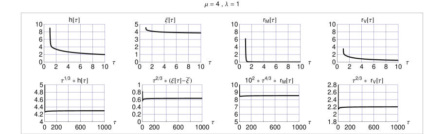
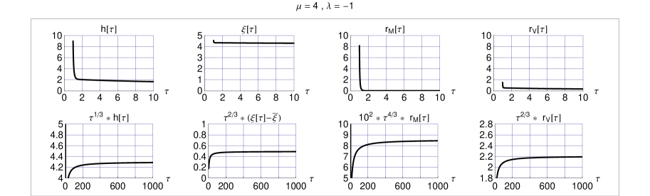
Figure 1: Numerical solution of the ODEs (15) with source term (17) and energy density (16a), for parameters $w_{M}=1/3$, $\mu=4$, $\lambda=1$, and $\widetilde{\gamma}=10^{-3}$. The boundary conditions at $\tau=\tau_{\text{bcs}}=1$ are $\{h,\,\xi,\,r_{M}\}=\{9,4.55,6.16616\}$, where the $r_{M}$ value has been obtained from the first Friedman equation (15e). The top row shows the three basic variables: the Hubble parameter $h=\dot{a}/a$, the dimensionless vacuum variable $\xi$, and the matter energy density $r_{M}$. The bottom row shows their asymptotic behavior: $h(\tau)\sim\tau^{-1/3}$, $\xi(\tau)-\overline{\xi}\sim\tau^{-2/3}$, $r_{M}(\tau)\sim\tau^{-4/3}$, and $r_{V}(\tau)\sim\tau^{-2/3}$, where $\overline{\xi}$ is given by (16c). Both rows show the corresponding vacuum energy density $r_{V}$ from (15e) and (16a).

Figure 2: Numerical solution of the ODEs (15) with source term (17) and energy density (16a), for parameters $w_{M}=1/3$, $\mu=4$, $\lambda=-1$, and $\widetilde{\gamma}=10^{-3}$. The boundary conditions at $\tau=\tau_{\text{bcs}}=1$ are $\{h,\,\xi,\,r_{M}\}=\{9,4.55,8.16616\}$, where the $r_{M}$ value has been obtained from the first Friedman equation (15e). The variables shown are explained in the caption of Fig. 2.

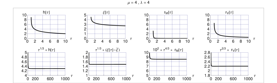
Figure 3: Numerical solution of the ODEs (15) with source term (17) and energy density (16a), for parameters $w_{M}=1/3$, $\mu=4$, $\lambda=4$, and $\widetilde{\gamma}=10^{-3}$. The boundary conditions at $\tau=\tau_{\text{bcs}}=1$ are $\{h,\,\xi,\,r_{M}\}=\{9,4.55,3.16616\}$, where the $r_{M}$ value has been obtained from the first Friedman equation (15e). The variables shown are explained in the caption of Fig. 2, but the asymptotic behavior of the dimensionless vacuum variable is now different: $\xi(\tau)-\overline{\xi}\sim\tau^{-1/3}$.

III.5 Discussion

Following-up on the attractor-domain discussion of the last subsection with numerical results, we emphasize that the analytic solution KlinkhamerVolovik-MPLA-2016 is clear about having a finite attractor domain. Let us give the details (expanding on the statement from the last paragraph of App. B in that reference): $\xi(\tau_{\text{bcs}})$ must be such as to make $r_{V}(\tau_{\text{bcs}})$ nonnegative and $h(\tau_{\text{bcs}})$ must also be nonnegative with a further condition that traces back to (15e). These conditions can be summarized as follows:

$$h(\tau_{\text{bcs}})\geq\sqrt{\frac{8\pi}{3}\,r_{V}(\tau_{\text{bcs}})}\geq 0\,.$$ (21)

How the actual attractor domain looks in the $\{h(\tau_{\text{bcs}}),\xi(\tau_{\text{bcs}})\}$ plane depends on the details of the Ansatz for $\widetilde{\epsilon}\,[\xi]$ and the numerical values of $\mu$ and $\lambda$, possibly obeying a condition similar to (16b). Incidentally, there is no such condition on $\lambda$, for given $\mu$, if the $\widetilde{\epsilon}$ Ansatz is changed to, for example, $\widetilde{\epsilon}\,[\xi]=(\xi^{2})^{1/4}+(\xi^{2})^{-1/4}$, which allows for the cancellation of any value of $\lambda\in\mathbb{R}$ for arbitrary $\mu$.

There is, however, a puzzle. Namely, the numerical results for $\mu=4$ and $\lambda=\pm 1$ in Figs. 2 and 2 show that Minkowski spacetime is approached, but how can that be as $\mu=4$ differs from the fine-tuned value $\mu_{0}$ for the Minkowski vacuum of Ref. KlinkhamerVolovik2008a ? Incidentally, for the $\widetilde{\epsilon}(\xi)$ Ansatz in (16a), the equilibrium value of the chemical potential is given by $\mu_{0}=2\,\sqrt{\lambda}$, provided $\lambda$ is nonnegative (all the more surprising that our numerical solution can approach Minkowski spacetime also for negative $\lambda$!).

The answer is simply that the Minkowski vacuum of Ref. KlinkhamerVolovik2008a holds for static fields, whereas our numerical solution is nonstatic, $\xi=\xi(\tau)$ with $\dot{\xi}\neq 0$.

The numerical results for $\mu=4$ and $\lambda=\pm 1$ do not appear to have a rigorous “limit” as $\tau\to\infty$ and the fields are essentially time-dependent. This is reminiscent of Dolgov’s model Dolgov1985 ; Dolgov1997 (see also Fig. 2  in Ref. KlinkhamerVolovik2010 and App. A in Ref. EmelyanovKlinkhamer2012 ), even though the time-dependence of $h=h(\tau)$ and $\xi=\xi(\tau)$ in our 4D-brane model diminishes with time, whereas Dolgov’s time-dependence stays constant with time (specifically, a linear time dependence of the massless vector field). Still, the final state with $q=\overline{q}$ is, in general, not the static-equilibrium state with $q=q_{0}$ and the question remains whether or not such a situation is acceptable (especially as concerns the gravitational dynamics of a solar-system-type subsystem; see Sec. I of Ref. EmelyanovKlinkhamer2012 for further discussion and references).

For the special case $\mu=4$ and $\lambda=4$, there may be a strict limit, as we then reach the genuine Minkowski vacuum of Ref. KlinkhamerVolovik2008a at $\mu_{0}=4$, with $\xi_{0}=2$ from (16c). The $\xi(\tau)$ values in Table 1 appear to approach the equilibrium value $\xi_{0}=2$. The corresponding dimensional vacuum variable $q(t)$ then approaches the equilibrium value $q_{0}$, around which the vacuum energy density has a quadratic behavior, $\rho_{V}(q)\sim c_{2}\,\big{(}q-q_{0}\big{)}^{2}$ with a positive constant $c_{2}$ of mass dimension $-4$ (here, $c_{2}\propto E_{\text{Planck}}^{-4}$).

Table 1: Function values from the numerical solution of Fig. 3, showing only 3 significant digits.

$\;\;\tau$	$h(\tau)$	$\xi(\tau)$	$r_{M}(\tau)$	$r_{V}(\tau)\;\;$
$\;\;10^{2}$	$0.926$	$2.32$	$1.85\times{10}^{-4}$	$0.102\;\;$
$\;\;10^{3}$	$0.430$	$2.15$	$8.55\times{10}^{-6}$	$0.0221\;\;$
$\;\;10^{4}$	$0.200$	$2.07$	$3.97\times{10}^{-7}$	$0.00476\;\;$
$\;\;10^{5}$	$0.0927$	$2.03$	$1.84\times{10}^{-8}$	$0.00102\;\;$
$\;\;10^{6}$	$0.0430$	$2.01$	$8.56\times{10}^{-10}$	$0.000221\;\;$

IV Outlook

The present paper has studied the cosmological behavior of a $q$-field in the 4D-brane realization KlinkhamerVolovik-JETPL-2016-4Dbrane . The physical interpretation of this $q$-field scalar relates to a four-dimensional number density $n$ of “spacetime atoms,” with a corresponding chemical potential $\mu$. This number density $n$ is a new variable, as the action (1) makes clear. It leads to an additional conservation equation (5) of the corresponding vacuum energy density $\rho_{V}(q)$.

A similar model has been presented recently Klinkhamer2022-ext-unimod-grav , where there is also a four-dimensional number density $n$ with a corresponding chemical potential $\mu$. But, in that case, there is no need for a new variable as $n$ is simply proportional to $\sqrt{-g}$, in terms of the already available metric determinant $g\equiv\det(g_{\alpha\beta})$. [This identification implies the restriction of the allowed coordinate transformations to those with unit Jacobian.] In that case, there is no additional conservation equation for $\rho_{V}$. Yet, in a cosmological context, the Friedmann equations do contain the equation $d\rho_{V}/dt=0$; see the last paragraph of Sec. VI B in Ref. Klinkhamer2022-ext-unimod-grav . Moreover, there appears an attractor behavior towards Minkowski spacetime provided there is vacuum-matter energy exchange.

Both manifestations of $n$ apparently involve some fine-scale underlying structure of spacetime, called “atoms of spacetime” for the 4D-brane realization KlinkhamerVolovik-JETPL-2016-4Dbrane and a “spacetime crystal” for the extended-unimodular-gravity approach Klinkhamer2022-ext-unimod-grav . The outstanding question is what the actual substructure of spacetime really is. A partial answer can perhaps be obtained from nonperturbative superstring theory as formulated by the IIB matrix model IKKT-1997 ; Aoki-etal-review-1999 ; Klinkhamer2021-master .

- (1) S. Weinberg, “The cosmological constant problem,” Rev. Mod. Phys. 61, 1 (1989).
- (2) F.R. Klinkhamer and G.E. Volovik, “Self-tuning vacuum variable and cosmological constant,” Phys. Rev. D 77, 085015 (2008), arXiv:0711.3170.
- (3) F.R. Klinkhamer and G.E. Volovik, “Dynamic vacuum variable and equilibrium approach in cosmology,” Phys. Rev. D 78, 063528 (2008), arXiv:0806.2805.
- (4) F.R. Klinkhamer and G.E. Volovik, “Towards a solution of the cosmological constant problem,” JETP Lett. 91, 259 (2010), arXiv:0907.4887.
- (5) E.I. Kats and V.V. Lebedev, “Nonlinear fluctuation effects in dynamics of freely suspended films,” Phys. Rev. E 91, 032415 (2015), arXiv:1501.06703.
- (6) F.R. Klinkhamer and G.E. Volovik, “Brane realization of -theory and the cosmological constant problem,” JETP Lett. 103, 627 (2016), arXiv:1604.06060.
- (7) F.R. Klinkhamer and G. E. Volovik, “Big bang as a topological quantum phase transition,” Phys. Rev. D 105, 084066 (2022), arXiv:2111.07962.
- (8) F.R. Klinkhamer, M. Savelainen and G.E. Volovik, “Relaxation of vacuum energy in -theory,” J. Exp. Theor. Phys. 125, 268 (2017), arXiv:1601.04676.
- (9) F.R. Klinkhamer and G.E. Volovik, “Dynamic cancellation of a cosmological constant and approach to the Minkowski vacuum,” Mod. Phys. Lett. A 31, 1650160 (2016), arXiv:1601.00601.
- (10) Ya.B. Zel’dovich and A.A. Starobinsky, “Rate of particle production in gravitational fields,” JETP Lett. 26, 252 (1977).
- (11) R. Bousso and J. Polchinski, “Quantization of four-form fluxes and dynamical neutralization of the cosmological constant,” JHEP 06, 006 (2000), arXiv:hep-th/0004134.
- (12) A.D. Dolgov, “Field model with a dynamic cancellation of the cosmological constant,” JETP Lett. 41, 345 (1985).
- (13) A.D. Dolgov, “Higher spin fields and the problem of cosmological constant,” Phys. Rev. D 55, 5881 (1997), arXiv:astro-ph/9608175.
- (14) V. Emelyanov and F.R. Klinkhamer, “Possible solution to the main cosmological constant problem,” Phys. Rev. D 85, 103508 (2012), arXiv:1109.4915.
- (15) F.R. Klinkhamer, “Extension of unimodular gravity and the cosmological constant,” Phys. Rev. D 106, 124015 (2022), arXiv:2207.02826.
- (16) N. Ishibashi, H. Kawai, Y. Kitazawa, and A. Tsuchiya, “A large- reduced model as superstring,” Nucl. Phys. B 498, 467 (1997), arXiv:hep-th/9612115.
- (17) H. Aoki, S. Iso, H. Kawai, Y. Kitazawa, A. Tsuchiya, and T. Tada, “IIB matrix model,” Prog. Theor. Phys. Suppl. 134, 47 (1999), arXiv:hep-th/9908038.
- (18) F.R. Klinkhamer, “IIB matrix model: Emergent spacetime from the master field,” Prog. Theor. Exp. Phys. 2021, 013B04 (2021), arXiv:2007.08485.