The isovector axial form factor of the nucleon from lattice QCD

Abstract

The isovector axial form factor of the nucleon plays a key role in interpreting data from long-baseline neutrino oscillation experiments. We perform a lattice-QCD based calculation of this form factor, introducing a new method to directly extract its $z$-expansion from lattice correlators. Our final parametrization of the form factor, which extends up to spacelike virtualities of $0.7\,{\rm GeV}^{2}$ with fully quantified uncertainties, agrees with previous lattice calculations but is significantly less steep than neutrino-deuterium scattering data suggests.

I Introduction

The axial form factor of the nucleon $G_{\rm A}(Q^{2})$ plays a central role in understanding the quasi-elastic part of GeV-scale neutrino-nucleus cross sections. Particularly for the upcoming long-baseline neutrino oscillation experiments DUNE Acciarri et al. (2015) and T2HK Abe et al. (2018), these cross sections must be known with few-percent uncertainties Ruso et al. (2022) to enable a sufficiently reliable reconstruction of the incident neutrino energy. In the absence of modern, high-quality experimental measurements of $G_{\rm A}(Q^{2})$ Bernard et al. (2002), calculations for the axial form factor from lattice QCD Meyer et al. (2022) are of crucial importance in order to maximize the scientific output of neutrino-oscillation experiments.

For a long time, the axial charge of the nucleon, $G_{\rm A}(0)$, served as a benchmark quantity for lattice QCD calculations Aoki et al. (2021), exemplifying the improvements of recent years in terms of control over statistical and systematic errors. The latter are caused mainly by the excited-state contamination in Euclidean correlation functions, as well as by the chiral and continuum extrapolation. Many of the techniques developed have been carried over and applied to non-vanishing momentum transfer $Q^{2}$, most recently in Refs. Park et al. (2022); Jang et al. (2020); Bali et al. (2020); Alexandrou et al. (2021); Shintani et al. (2019); Ishikawa et al. (2021). In comparison to the calculation of the charge, a new source of systematics arises for the form factor, namely the parameterization of the $Q^{2}$-dependence. Historically, an ad hoc dipole ansatz was used (see Bernard et al. (2002)), incurring an unquantified model systematic. As a modern alternative, an ansatz based on the $z$-expansion has been used extensively, leading to less model bias at the cost of an increased statistical error on the phenomenological determination of the mean square radius $\langle r_{\rm A}^{2}\rangle=[\frac{-6}{G_{\rm A}}\frac{dG_{\rm A}}{dQ^{2}}]_{Q^{2}=0}$ Hill et al. (2018). The sensitivity to the parameterization is also visible in lattice calculations, where the different ansätze lead to inconsistent results (see e.g. Bali et al. (2020)).

In this Letter, we perform a high-statistics calculation of $G_{\rm A}(Q^{2})$ for momentum transfers up to $0.7\,{\rm GeV}^{2}$ using lattice simulations with dynamical up, down and strange quarks with an O($a$) improved Wilson fermion action. We employ a new analysis method that simultaneously handles the issues of the excited-state contamination and the description of the form factor’s $Q^{2}$ dependence.

II Methodology

The matrix elements of the local iso-vector axial current $A^{a}_{\mu}(x)=\bar{\psi}\gamma_{\mu}\gamma_{5}\frac{\tau^{a}}{2}\psi$ between single-nucleon states are parameterized by the axial form factor $G_{\rm A}(Q^{2})$ and induced pseudoscalar form factor $G_{\rm P}(Q^{2})$. We focus on the current component orthogonal to the momentum transfer, thereby projecting out the axial form factor,

$$\langle N(p^{\prime},s^{\prime})|\,\vec{q}\times\vec{A}^{a}(0)\,|N(p,s)\rangle=$$

$$\qquad G_{\rm A}(Q^{2})\;\bar{U}^{s^{\prime}}(p^{\prime})\,\vec{q}\times\vec{\gamma}\;\gamma_{5}\,{\textstyle\frac{\tau^{a}}{2}}U^{s}(p),$$

where $\vec{q}=\vec{p}^{\,\prime}-\vec{p}$, $Q^{2}=\vec{q}{\,}^{2}-(E_{\vec{p}^{\prime}}-E_{\vec{p}})^{2}$ and $U^{s}(p)$ is an isodoublet Dirac spinor with momentum $p$ and spin state $s$. We employ Euclidean notation throughout.

The setup for our lattice determination of the axial form factor is very similar to the one we used in the case of the electromagnetic form factors Djukanovic et al. (2021). The nucleon two- and three-point functions are computed as

$$C_{2}(\vec{p},t) = a^{3}\sum_{\vec{x}}e^{i\vec{p}\cdot\vec{x}}\,\Gamma_{\beta\alpha}\,\Big{\langle}\Psi^{\alpha}(t,\vec{x})\overline{\Psi}^{\beta}(0)\Big{\rangle},$$ (2)

$$C_{3}(\vec{q},t,t_{s}) = -i\,a^{6}\sum_{\vec{x},\vec{y}}e^{i\vec{q}\cdot\vec{y}}\,\Gamma_{\beta\alpha}\,\frac{\vec{q}\times\vec{s}}{|\vec{q}\times\vec{s}|^{2}}\cdot$$

$$\Big{\langle}\Psi^{\alpha}(t_{s},\vec{x})\,\vec{q}\times\!\vec{A}^{a=3}(t,\vec{y})\,\overline{\Psi}^{\beta}(0)\Big{\rangle},$$

where $\Psi^{\alpha}(\vec{x},t)$ denotes the proton interpolating operator

$$\Psi^{\alpha}(x)=\epsilon_{abc}\big{(}\tilde{u}^{T}_{a}(x)C\gamma_{5}\tilde{d}_{b}(x)\big{)}\tilde{u}^{\alpha}_{c}(x).$$ (4)

The quark fields $\tilde{u},\tilde{d}$ are smeared with a Gaussian kernel Güsken, S. and Löw, U. and Mütter, K. H. and Sommer, R. and Patel, A. and Schilling, K. (1989), using APE-smeared gauge fields Albanese et al. (1987). Note that the nucleon three-point function is computed in the rest frame of the final-state nucleon, $\vec{p}^{\,\prime}=0$, and the chosen projection matrix $\Gamma$ reads

$$\Gamma={\textstyle\frac{1}{2}}(1+\gamma_{0})(1+i\gamma_{5}\vec{s}\cdot\vec{\gamma}).$$ (5)

In practice, we have set $\vec{s}=\vec{e}_{3}$, i.e. the nucleon spin is aligned along the $x_{3}$-axis. When averaging over equivalent momenta we find an improved signal using the constraint $|q_{3}|\leq\min\Bigl{(}|q_{1}|,|q_{2}|\Bigr{)}$. The transverse part $\vec{q}\times\!\vec{A}^{a}$ of the axial current receives no additive O($a$) improvement. For its multiplicative renormalization, we employ the determination of $Z_{A}$ and $b_{A}$ from Dalla Brida et al. (2019) and Korcyl and Bali (2017), respectively, while the coefficient $\tilde{b}_{A}$ in the notation of Korcyl and Bali (2017) is neglected, since it parametrizes a sea-quark effect and is expected to be small.

We use the ratio

$$R(\vec{q},t,t_{s})\equiv\frac{C_{3}(\vec{q},t,t_{s})}{C_{2}(0,t_{s})}\sqrt{\frac{C_{2}(\vec{q},t_{s}-t)C_{2}(\vec{0},t)C_{2}(\vec{0},t_{s})}{C_{2}(\vec{0},t_{s}-t)C_{2}(\vec{q},t)C_{2}(\vec{q},t_{s})}}$$ (6)

to build the summed insertion

$$S(\vec{q},t_{s}) \equiv a\,\sqrt{\frac{2E_{\vec{q}}}{m+E_{\vec{q}}}}\;\sum_{t=a}^{t_{s}-a}R(\vec{q},t,t_{s})$$

$$\stackrel{{\scriptstyle t_{s}\to\infty}}{{=}} b_{0}(\vec{q})+t_{s}G_{\rm A}(Q^{2})+\dots$$

The dots stand for excited-state contributions that are of order $t_{s}e^{-\Delta t_{s}}$, with $\Delta$ the energy gap above the single-nucleon state. As a novelty, we introduce a technique which is based on fitting the quantities $S(\vec{q},t_{s})$ simultaneously for different $\vec{q}$ and $t_{s}$, by parameterizing the axial form factor from the outset via the $z$-expansion (see Hill et al. (2018); Hill and Paz (2010) and Refs. therein),

$$G_{\rm A}(Q^{2}) = \sum^{n_{\rm max}}_{n=0}a_{n}\,z^{n}(Q^{2})\,,$$ (8)

$$z(Q^{2}) = \frac{\sqrt{t_{\rm cut}+Q^{2}}-\sqrt{t_{\rm cut}}}{\sqrt{t_{\rm cut}+Q^{2}}+\sqrt{t_{\rm cut}}}\;.$$ (9)

The fit parameters are the coefficients $a_{n}$ and the offsets $b_{0}(\vec{q})$, which we keep as independent fit parameters for each $\vec{q}$. In the data analyzed below, we set $n_{\rm max}=2$ without constraining the fit parameters by priors. We note that setting $n_{\rm max}=3$ would require the use of priors for the highest-order term to stabilize the fit, but the results are consistent with our preferred $n_{\rm max}=2$ results. To obtain the form factor at the physical point, the $a_{n}$ are extrapolated to the continuum and interpolated to the physical pion mass, at which point the form factor may be evaluated at any virtuality in the chosen expansion interval $[0,\;0.7\,{\rm GeV}^{2}]$.

Our method relies on the fact that, for a given $Q^{2}$-interval, the $z$-expansion represents a general, systematically improvable parameterization of the form factor Hill and Paz (2010). We have chosen to map $Q^{2}=0$ to the point $z=0$ and set $t_{\rm cut}=(3M_{\pi}^{\rm phys})^{2}$ to the three-pion kinematic threshold at the physical pion mass for all gauge ensembles used, as this choice facilitates the chiral extrapolation of the $a_{n}$. We find that the immediate parameterization of the form factor has a stabilizing effect as compared to the standard two-step procedure of first obtaining the form factor independently at discrete values of $\vec{q}$, followed by a continuous parameterization of these data points.

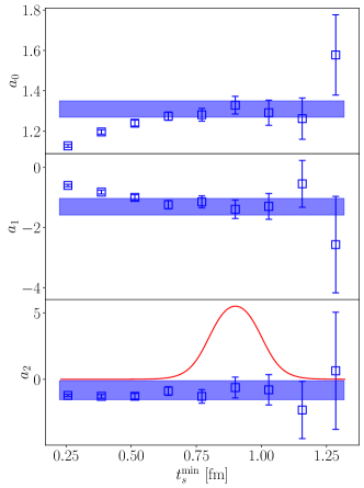
Figure 1: Illustration of averaging over the minimum source-sink separation $t_{s}^{\mathrm{min}}$ in the summation method for the near-physical pion mass ensemble E250 of size $192\times 96^{3}$ with a lattice spacing of 0.064 fm Bruno et al. (2017). We perform the $z$-expansion fits for each ensemble starting at different values of $t_{s}^{\mathrm{min}}$. The results for coefficients $a_{0}$, $a_{1}$ and $a_{2}$ are shown here as the blue squares. The bands represent the smooth-window averages over $t_{s}^{\mathrm{min}}$, and the solid red line shows the weight function Eq. (10) (multiplied by ten for clarity).

We perform fits to $S(\vec{q},t_{s})$ based on the second line of Eq. (II), dropping the omitted terms, and including all values of $t_{s}$ greater than or equal to a certain $t_{s}^{\textrm{min}}$. At small values of $t_{s}$, contributions from excited states are expected to be significant, whereas at large $t_{s}$ the signal-to-noise ratio becomes poor. This leaves us with a relatively small window of starting values $t_{s}^{\textrm{min}}$ that can safely be used. Rather than choosing a single $t_{s}^{\textrm{min}}$, we average the fit results over $t_{s}^{\textrm{min}}$ using as a weight factor the ‘smooth window’ function

$$\frac{1}{{\cal N}_{w}}\left[\tanh{\left(\frac{t_{s}^{\textrm{min}}-t_{w}^{\textrm{low}}}{\Delta t_{w}}\right)}-\tanh{\left(\frac{t_{s}^{\textrm{min}}-t_{w}^{\textrm{up}}}{\Delta t_{w}}\right)}\right]$$ (10)

with $t_{w}^{\textrm{low}}=0.8$ fm, $t_{w}^{\textrm{up}}=1.0$ fm and $\Delta t_{w}=0.08$ fm. The weights are normalized by ${\cal N}_{w}$ so as to add up to unity. The average represents very well what could be identified as a plateau in the fit results, as illustrated in Fig. 1. The three panels also illustrate the advantage of having to scrutinize only very few observables for excited-state effects, as opposed to having to do this for every $Q^{2}$ value. Having an extended set of $t_{s}$ values at our disposal, the control over these effects is significantly improved as compared to our previous summation-method results for the vector form factors Djukanovic et al. (2021).

III The lattice calculation

We use a set of fourteen CLS $N_{f}=2+1$ ensembles Bruno et al. (2015) that have been generated with non-perturbatively $\mathcal{O}(a)$-improved Wilson fermions Sheikholeslami and Wohlert (1985); Bulava and Schaefer (2013) and the tree-level improved Lüscher-Weisz gauge action Lüscher, M. and Weisz, P. (1985). They cover the range of lattice spacings from $0.050$ fm to $0.086$ fm and pion masses from about $350~{}\textrm{MeV}$ down to $130~{}\textrm{MeV}$. For most of these ensembles, the fields obey open boundary conditions in time Lüscher, Martin and Schaefer, Stefan (2011) in order to prevent topological freezing Schaefer et al. (2011). The reweighting factors needed to correct for the treatment of the strange-quark determinant during the gauge field generation were computed using the method of Ref. Mohler and Schaefer (2020). Our setup to compute the nucleon two- and three-point functions is similar to that used in our study on the isovector charges of the nucleon Harris et al. (2019).

As discussed in section II, we perform simultaneous fits to all data points with $Q^{2}\leq 0.7~{}\textrm{GeV}^{2}$ and source-sink separations $t_{s}\geq t_{s}^{\textrm{min}}$ on each ensemble to obtain the coefficients $a_{i}$ of the $z$-expansion at the given pion mass, lattice spacing and volume. Ensemble-by-ensemble results are compiled in the Supplementary Material. We then proceed to perform chiral and continuum extrapolations of the coefficients $a_{i}$ to the physical point, including for each of them a term linear in $a^{2}$. As for their chiral behaviour, we use the following three ansätze:

1. Linear in $M_{\pi}^{2}$ for all coefficients $a_{i}$.

2. Again linear in $M_{\pi}^{2}$ for coefficients $a_{1}$ and $a_{2}$, and an extended ansatz containing a chiral logarithm for the zeroth coefficient:

   $$a_{0}=g_{a}^{(0)}+g_{a}^{(1)}M_{\pi}^{2}+g_{a}^{(3)}M_{\pi}^{3}-g_{a}^{(2)}M_{\pi}^{2}\ln{\frac{M_{\pi}}{M_{n}}}$$

   with

   $$g_{a}^{(1)} =4d_{16}-\frac{(g_{a}^{(0)})^{3}}{16\pi^{2}F_{\pi}^{2}},$$

   $$g_{a}^{(2)} =\frac{g_{a}^{(0)}}{8\pi^{2}F_{\pi}^{2}}\left(1+2(g_{a}^{(0)})^{2}\right),$$

   $$g_{a}^{(3)} =\frac{g_{a}^{(0)}}{8\pi F_{\pi}^{2}M_{n}}\left(1+(g_{a}^{(0)})^{2}\right)-\frac{g_{a}^{(0)}}{6\pi F_{\pi}^{2}}\Delta_{c_{3},c_{4}},$$

   where $M_{n}=938.92~{}\textrm{MeV}$ is the nucleon mass and $F_{\pi}=92.42~{}\textrm{MeV}$ the pion decay constant Schindler et al. (2007). Here $\Delta_{c_{3},c_{4}}=c_{3}-2c_{4}$ is a combination of low-energy constants $c_{3}$ and $c_{4}$. The free fit parameters for the zeroth coefficient’s chiral extrapolation are $g_{a}^{(0)}$, $d_{16}$ and $\Delta_{c_{3},c_{4}}$.

3. Same as ansatz 2, but including $M_{\pi}^{3}$ terms for coefficients $a_{1}$ and $a_{2}$.

Note that, while the coefficients $a_{i}$ do not have common fit parameters, they are correlated within an ensemble: these correlations are taken into account in the fits. If the resulting correlation matrix is larger than $70\times 70$, we damp the off-diagonal correlations by 0.5%…1.5% to avoid numerical instabilities Touloumis (2015).

We perform multiple extrapolations using the different fit ansätze described above with pion mass cuts $M_{\pi}<M_{\pi}^{\rm cut}$ with $M_{\pi}^{\rm cut}[{\rm MeV}]\in\{300,\,285,\,265,\,250\}$, as well as dropping data from the coarsest lattice spacing, to get a handle on systematic effects. Although we do not observe a strong dependence on the volume, we include a term Beane and Savage (2004)

$$\frac{M_{\pi}^{2}}{\sqrt{M_{\pi}L}}\mathrm{e}^{-M_{\pi}L}$$ (11)

for the zeroth coefficient $a_{0}$ to check for possible finite-size effects (FSE) in some of the extrapolation fits. For a subset of fits, we impose Gaussian priors on the coefficients multiplying the $a^{2}$ terms, restricting the difference between the values at the coarsest lattice spacing and in the continuum limit to at most 20%. This is motivated by a tendency of these fits to attribute unnaturally large corrections to discretization effects, especially for $a_{1}$ and $a_{2}$ that are statistically less precise. We keep those fits that have a $p\,$-value better than 5% and provide a satisfactory description of the data, especially at pion masses below 200 MeV.

Some examples of these fits based on different ansätze and pion mass cuts are shown in the Supplementary Material. While most of our fits have a good $p\,$-value without including the FSE term of Eq. (11), which tends to slightly increase the uncertainties, we do include these fits in the analysis in order to account for the systematic effect due to finite-size corrections. We can also inspect finite-size effects directly by comparing our results of the $z$-expansion fits on two ensembles at a pion mass of $280\,\textrm{MeV}$, H105 and N101, which differ only by their spatial sizes, $L=2.8\,$fm and 4.1 fm respectively. We find that the coefficients $a_{i}$ agree well, confirming that finite-size effects are small at the current level of precision.

Since different fit ansätze and cuts can be equally well motivated, as in our previous study of the vector form factors of the nucleon Djukanovic et al. (2021) we perform a weighted average Jay and Neil (2021) over the resulting $a_{i}$, where the Akaike Information Criterion (AIC) Akaike (1974) is used to weight different analyses and to estimate the systematic error associated with the variations of the global fit. Different versions of the AIC weights have been developed and used over the years. Here we choose Borsanyi et al. (2021)

$$w^{\textrm{AIC}}=N\mathrm{e}^{-\frac{1}{2}\left(\chi^{2}+2n_{\textrm{par}}-n_{\textrm{data}}\right)},$$ (12)

where the minimum $\chi^{2}$, the number of fit parameters $n_{\textrm{par}}$ and the number of data points $n_{\textrm{data}}$ characterize the fit. $N$ is a normalization factor that ensures that the sum of the weights is unity. The corresponding cumulative distribution functions of the coefficients $a_{i}$ and of the mean square radius $\langle r_{A}^{2}\rangle$ are well-behaved and show no outliers. We determine the central value from the 50th percentile, and the full uncertainty as the interval from the 16th to the 84th percentile. The decomposition of the error into its statistical and systematic components is achieved following the prescription proposed in Borsanyi et al. (2021).

IV Results

Our results for the coefficients of the $z$-expansion of the nucleon axial form factor in the continuum and at the physical pion mass are

$$a_{0}= \quad\>1.225\pm 0.039\textrm{ (stat)}\pm 0.025\textrm{ (syst)},$$

$$a_{1}= -1.274\pm 0.237\textrm{ (stat)}\pm 0.070\textrm{ (syst)},$$

$$a_{2}= -0.379\pm 0.592\textrm{ (stat)}\pm 0.179\textrm{ (syst)}$$ (13)

with a correlation matrix

$$M_{\textrm{corr}}=\left(\!\begin{array}[]{rrr}1.00000&-0.67758&0.61681\\ -0.67758&1.00000&-0.91219\\ 0.61681&-0.91219&1.00000\end{array}\,\right).$$ (14)

These results, meant to be inserted into Eqs. (8–9) with $t_{\rm cut}=(3M_{\pi^{0}})^{2}$, lead to the following mean square radius,

$$\langle r^{2}_{A}\rangle = (0.370\pm 0.063\textrm{ (stat)}\pm 0.016\textrm{ (syst)})~{}\textrm{fm}^{2}.~{}~{}~{}~{}$$ (15)

We compare our result to other lattice QCD determinations of the mean square radius in Fig. 2, finding good agreement. The comparison features only lattice calculations with a full error budget, including a continuum extrapolation; see Refs. Jang et al. (2020); Alexandrou et al. (2021); Shintani et al. (2019); Ishikawa et al. (2021); Hasan et al. (2018) for further lattice results. The NME21 result is from Park et al. (2022), and the RQCD19 result is from Bali et al. (2020). Both studies parameterize the $Q^{2}$ dependence of the form factor using a $z$-expansion (RQCD also use a dipole ansatz as an alternative parameterization, but that result is not shown in the figure). For comparison, we show the average of the values obtained from $z$-expansion fits to neutrino scattering and muon capture measurements Hill et al. (2018). Our result also agrees well with the earlier two-flavour calculation by the Mainz group Capitani et al. (2019), and with a more recent analysis Schulz et al. (2022) by the same group that has been obtained via the conventional two-step process of first determining the form factor at discrete $Q^{2}$ values and subsequently parameterizing it.

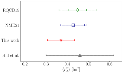
Figure 2: Comparison of lattice determinations of the mean square radius $\langle r_{\text{A}}^{2}\rangle$, from Refs. Park et al. (2022) (NME21) and Bali et al. (2020) (RQCD19). The point labeled Hill et al. is an average of the values obtained from $z$-expansion fits to neutrino scattering and muon capture Hill et al. (2018). The smaller error bars with solid lines show the statistical errors, whereas the wider error bars with dashed lines show the total errors (including systematic uncertainties).

Perhaps even more interesting is the comparison of our result for the axial form factor to data from pion electroproduction experiments Bernard et al. (2002) and to a $z$-expansion fit to neutrino-Deuterium scattering data Meyer et al. (2016) in Fig. 3. Our result agrees well with other lattice QCD calculations, as can be seen by comparing this figure to Fig. 3 in the review Meyer et al. (2022), but there is a tension with the axial form factor extracted from experimental deuterium bubble chamber data Meyer et al. (2016). This tension is strongest at large $Q^{2}$, the deuterium extraction being lower than the lattice prediction. The authors of the Snowmass White Paper on Neutrino Scattering Measurements Alvarez-Ruso et al. (2022) remark that, when translated to the nucleon quasielastic cross section, this discrepancy suggests that a 30-40% increase would be needed for these two results to match. They also note that recent high-statistics data on nuclear targets cannot directly resolve such discrepancies due to nuclear modeling uncertainties, and that new elementary target neutrino data would provide a critical input to resolve such discrepancies.

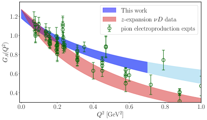
Figure 3: Comparing our result for the axial form factor to data from pion electroproduction experiments Bernard et al. (2002) and to a $z$-expansion fit to neutrino-Deuterium scattering data Meyer et al. (2016). There is a clear tension between the lattice QCD result and the $z$-expansion extracted from deuterium bubble chamber data, especially at large $Q^{2}$. The darker blue error band highlights the $Q^{2}$ range of our lattice data. The data from electroproduction experiments has been multiplied by the current PDG value for the axial charge Workman et al. .

V Conclusions

In this Letter we have introduced a new method to extract the axial form factor of the nucleon. It combines two well-known methods into one analysis step: the summation method ensures that excited-state effects are sufficiently suppressed, and the $z$-expansion readily provides the parameterization of the $Q^{2}$ dependence of the form factor. Our main results are the coefficients of the $z$-expansion, given in Eq. (13). Systematic effects are included through AIC averaging, which also provides the break-up into statistical and systematic uncertainties and the correlations among the coefficients. Our results are statistics-limited, implying that significant improvements are still straightforwardly possible, though computationally costly.

We observe good agreement with other lattice QCD determinations of the axial form factor, which means that the tension with the shape of the form factor extracted from deuterium bubble chamber data is further strengthened. Comparing our result for $a_{0}\equiv G_{\rm A}(0)$ to the Particle Data Group (PDG) value for the axial charge, $g_{A}=1.2754(13)$ Workman et al. , which one might view as a benchmark, we find agreement at the $1.1\,\sigma$ level. Also, using largely the same gauge ensembles as in this work, we have previously found a good overall agreement for the isovector vector form factors Djukanovic et al. (2021) with phenomenological determinations, which are far more precise than in the axial-vector case. Thus a nucleon axial form factor falling off less steeply than previously thought now appears more likely.

In the near future, we plan to perform a dedicated calculation of various forward nucleon matrix elements, including the axial charge, updating the results of Ref. Harris et al. (2019).

Supplementary material

In order to further document our results, we provide additional figures illustrating a few specific aspects of the analysis, and expand on certain technical details.

V.1 Lattice ensembles

As explained in the main text, we use the CLS $N_{f}=2+1$ ensembles Bruno et al. (2015) that have been generated with non-perturbatively $\mathcal{O}(a)$-improved Wilson fermions Sheikholeslami and Wohlert (1985); Bulava and Schaefer (2013) and the tree-level improved Lüscher-Weisz gauge action Lüscher, M. and Weisz, P. (1985). The lattice spacings of these ensembles, lattice volumes, pion and nucleon masses, as well as the number of configurations, of measurements and of available source-sink separations $t_{s}$, are listed in Table 1. All lattices used in this study have a fairly large volume, which is indicated by $M_{\pi}L\gtrsim 4$.

V.2 Method

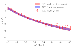
Figure 4: Illustration of the new method. We plot the results of fits to single $Q^{2}$ data (red data points) and compare them to the result of the immediate $z$-expansion (the blue error band) on ensemble E250 using $t_{s}^{\textrm{min}}=12$. The red error band is a $z$-expansion fit to the single $Q^{2}$ data points (including correlations), whereas the blue error band shows the fit where the $z$-expansion is directly incorporated into the summation method (Eq. (II)). Here $t_{s}^{\textrm{min}}=12$. The agreement is good, and the immediate $z$-expansion provides readily a model-independent parameterization of the shape of the form factor.

In our analysis, we incorporate the $z$-expansion, which parameterizes the $Q^{2}$ dependence of the form factor, directly into the summation method. This can also be done in two separate steps, first using the summation method to get the value of the form factor at a given $Q^{2}$, keeping track of the correlation between the data at different $Q^{2}$ values, and then parameterizing the $Q^{2}$ dependence of the form factor using a $z$-expansion. The two methods should obviously give compatible results, which we find to be the case. This is illustrated in Fig. 4 on ensemble E250. The first method leads to larger correlation matrices, which is why we have to damp the off-diagonal elements in some cases (for matrices larger than $70$) by 0.5%…1.5%. However, the one-step fits are very stable and robust, and the damping of off-diagonal correlations essentially only affects the $\chi^{2}$ of the fit. This is our preferred method, as it gives readily a parameterization of the shape of the form factor. The results of these fits are tabulated in Table 2 ensemble-by-ensemble.

V.3 Extrapolation to physical point and FSE

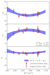
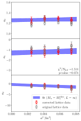
Figure 5: Chiral and continuum extrapolations using fit ansatz 3 (without the FSE term) and a pion mass cut of 300 MeV. The red circles show the corrected lattice data at infinite volume, and with zero lattice spacing or physical pion mass respectively in the left and right columns, whereas the grey data points are uncorrected.

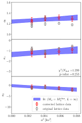
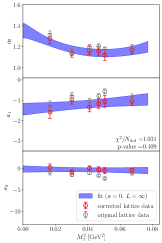
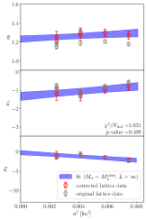
Figure 6: Extrapolation in pion mass and lattice spacing using fit ansatz 3 (top panel) and fit ansatz 2 (lower panel) with a pion mass cut of 265 MeV. No FSE term was included in these fits. The red circles show the corrected lattice data at infinite volume, and with zero lattice spacing or physical pion mass respectively in the left and right columns, whereas the grey data points are uncorrected.

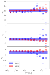
Figure 7: Direct comparison of the data as a function of $t_{s}^{\mathrm{min}}$ and the ’smooth window’ average of Eq. (10) on two of the ensembles, H105 and N101. These ensembles have the same lattice spacing and quark masses, but differ by their volume. The data points show good agreement, which indicates that any finite size effects are small.

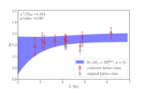
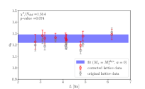
Figure 8: Finite size effects: coefficient $a_{0}$ (the axial charge) from fit ansatz 3 with a pion mass cut of 300 MeV, with and without the FSE term (Eq. (11)). The two fits are equally good, and are both included in the AIC average.

We include global fits with three different ansätze for the chiral behaviour of the form factor and several pion mass cuts in our final AIC average. We also take into account finite volume corrections by including a volume-dependent term (Eq. (11) in the main text) in some of our fits. We show examples of these global fits in Figs. 5, 6 and 8. Fig. 6 highlights the difference between ansatz 2 and ansatz 3, whereas comparing Fig. 5 and the top panel of Fig. 6 shows ansatz 3 with different pion mass cuts (300 MeV and 265 MeV, respectively). Fig. 8 compares a selected fit, ansatz 3 with a pion mass cut of 300 MeV, with and without the FSE term. At present statistics, the effect of adding the FSE term to the fit is almost negligible. Doing a more direct comparison of finite volume effects by looking at two ensembles, N101 and H105, which differ only by their volume, confirms this. We show the results of the $z$-expansion fits on these two ensembles as a function of $t_{s}^{\textrm{min}}$ in Fig. 7. We find that the coefficients $a_{i}$ are consistent between the two ensembles, and observe no significant finite size effects.

V.4 Akaike (AIC) model average

In this section, we give more details of the final step of the analysis, the AIC model average. As discussed in section III, we take systematic errors into account by performing an Akaike-information-criterion based average over a set of chiral, continuum and infinite-volume extrapolations. We choose the weight Borsanyi et al. (2021)

$$w^{\textrm{AIC}}_{k}=N\mathrm{e}^{-\frac{1}{2}\left(\chi^{2}_{k}+2n_{\textrm{par},k}-n_{\textrm{data},k}\right)},$$

where the $\chi^{2}_{k}$, the number of fit parameters $n_{\textrm{par},k}$ and the number of data points $n_{\textrm{data},k}$ describe the $k$-th global fit. The first two terms in the exponent correspond to the standard AIC, and the last term is introduced to take into account fits with different number of data points, i.e. fits with different cuts in pion mass or lattice spacing. The weights are normalized so that $\sum_{i}w_{i}=1$.

The weights $w^{\textrm{AIC}}_{i}$ are interpreted as propabilities, and the analyses follow a normal (Gaussian) distribution $N(a_{i};m_{k},\sigma_{k})$ with a central value $m_{k}$ and a standard deviation $\sigma_{k}$ for the quantity $a_{i}$. $m_{k}$ and $\sigma_{k}$ are the jackknife average and the jackknife error in the $k$-th analysis. A joint distribution function can then be defined as

$$\sum_{k}w^{\textrm{AIC}}_{k}N(a_{i};m_{k},\sigma_{k}),$$

which includes both statistical and systematic uncertainties. The corresponding cumulative distribution function reads

$$P(a_{i})=\int_{-\infty}^{a_{i}}\mathrm{d}a_{i}^{\prime}\sum_{k}w^{\textrm{AIC}}_{k}N(a_{i}^{\prime};m_{k},\sigma_{k}).$$

The median of the CDF gives the central value of $a_{i}$ and its total error is given by the 16% and 84% percentiles of the CDF. Noticing that scaling $\sigma_{k}$ by a factor of $\sqrt{\lambda}$ scales the statistical error by $\sqrt{\lambda}$, but does not scale the systematic error, using $\lambda=1$ and $\lambda=2$ allows us to calculate the break-up of the total uncertainty into statistical and systematic parts.

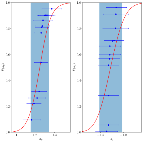
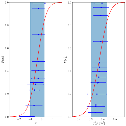
Figure 9: AIC average and the corresponding cumulative distribution function for all coefficients $a_{0}$, $a_{1}$, $a_{2}$, and the mean square radius $\langle r_{A}^{2}\rangle$ (in fm² units).

In Fig. 9, we show the AIC averages and the corresponding cumulative distributions for all coefficients $a_{i}$ as well as for the mean square radius $\langle r_{A}^{2}\rangle$. These are all well-behaved and contain no outliers. The data points are individual analyses, or fits, that give a good description of the data with a $p\,$-value better than 5%. These are the analyses that enter the AIC procedure. The error band shows the AIC average with the total (statistical and systematic) uncertainty.

ID	$\beta$	$T/a$	$L/a$	$M_{\pi}~{}[\textrm{MeV}]$	$M_{\pi}L$	$M_{N}~{}[\textrm{GeV}]$	$N_{\mathrm{conf}}$	$N_{\mathrm{meas}}$	$t_{s}~{}[\textrm{fm}]$	$N_{t_{s}}$
H102	3.40	96	32	354	4.96	1.103	2005	32080	0.35..1.47	14
H105	3.40	96	32	280	3.93	1.045	1027	49296	0.35..1.47	14
C101	3.40	96	48	225	4.73	0.980	2000	64000	0.35..1.47	14
N101	3.40	128	48	281	5.91	1.030	1596	51072	0.35..1.47	14
S400	3.46	128	32	350	4.33	1.130	2873	45968	0.31..1.53	9
N451	3.46	128	48	286	5.31	1.045	1011	129408	0.31..1.53	9
D450	3.46	128	64	216	5.35	0.978	500	64000	0.31..1.53	17
N203	3.55	128	48	346	5.41	1.112	1543	24688	0.26..1.41	10
N200	3.55	128	48	281	4.39	1.063	1712	20544	0.26..1.41	10
D200	3.55	128	64	203	4.22	0.966	2000	64000	0.26..1.41	10
E250	3.55	192	96	129	4.04	0.928	400	102400	0.26..1.41	10
N302	3.70	128	48	348	4.22	1.146	2201	35216	0.20..1.40	13
J303	3.70	192	64	260	4.19	1.048	1073	17168	0.20..1.40	13
E300	3.70	192	96	174	4.21	0.962	570	18240	0.20..1.40	13

Table 1: Overview of ensembles used in this study. The values $\beta=3.40$, $3.46$, $3.55$ and $3.70$ correspond to lattice spacings $a\approx 0.086$, $0.076$, $0.064$ and $0.05~{}\textrm{fm}$, respectively. Columns $T/a$ and $L/a$ give the temporal and spatial size of the lattice, and $M_{\pi}$ and $M_{N}$ are the pion and nucleon masses. $N_{\mathrm{conf}}$ is the number of configurations used for each ensemble, and in column $N_{\mathrm{meas}}$ we list the maximum number of measurements done per $t_{s}$ at largest source-sink separations ($>1.0~{}\textrm{fm}$). To keep the signal-to-noise ratio as a function of $t_{s}$ close to constant, the number of measurements is reduced by a factor of two in steps of $\Delta t_{s}\approx 0.2~{}\textrm{fm}$ for $t_{s}<1.0~{}\textrm{fm}$. $N_{t_{s}}$ is the number of available source-sink separations in the range listed in column $t_{s}$. However, in this study we restrict the smallest value of $t_{s}$ included in the summation method, $t_{s}^{\textrm{min}}$, to be in the range $0.8..1.0~{}\textrm{fm}$ using the smooth window (see Eq. (10)).

ID	$a_{0}$	$a_{1}$	$a_{2}$	$\rho_{a_{0},a_{1}}$	$\rho_{a_{0},a_{2}}$	$\rho_{a_{1},a_{2}}$
C101	$1.177(20)$	$-0.56(12)$	$-2.36(29)$	$-0.59707$	$0.30568$	$-0.85694$
D200	$1.193(28)$	$-1.07(17)$	$-1.01(42)$	$-0.58273$	$0.35465$	$-0.87957$
D450	$1.205(20)$	$-0.78(11)$	$-1.68(30)$	$-0.52813$	$0.13464$	$-0.76168$
E250	$1.310(40)$	$-1.31(28)$	$-0.82(72)$	$-0.61384$	$0.29885$	$-0.87065$
E300	$1.151(29)$	$-0.81(19)$	$-1.48(48)$	$-0.58834$	$0.31474$	$-0.88040$
H102	$1.157(16)$	$-0.55(11)$	$-2.01(33)$	$-0.39306$	$0.12100$	$-0.89438$
H105	$1.199(52)$	$-0.63(42)$	$-2.8(1.1)$	$-0.55469$	$0.33040$	$-0.93019$
J303	$1.188(33)$	$-0.89(20)$	$-1.05(52)$	$-0.59229$	$0.24273$	$-0.84407$
N101	$1.216(15)$	$-0.899(86)$	$-1.43(21)$	$-0.55315$	$0.22582$	$-0.81047$
N200	$1.247(35)$	$-0.71(21)$	$-1.76(54)$	$-0.53414$	$0.24793$	$-0.86773$
N203	$1.123(23)$	$-0.66(13)$	$-1.54(35)$	$-0.48820$	$0.18570$	$-0.83382$
N302	$1.164(34)$	$-0.64(26)$	$-2.36(70)$	$-0.48779$	$0.21775$	$-0.91619$
N451	$1.243(16)$	$-0.912(99)$	$-1.15(26)$	$-0.54656$	$0.27504$	$-0.84718$
S400	$1.178(23)$	$-0.47(18)$	$-1.99(51)$	$-0.44271$	$0.18507$	$-0.91340$

Table 2: Our results for the coefficients $a_{0}$, $a_{1}$, $a_{2}$ of the $z$-expansion for each ensemble, as well as their correlations $\rho_{a_{i},a_{j}}=(\langle a_{i}a_{j}\rangle-\langle a_{i}\rangle\langle a_{j}\rangle)/(\sqrt{\langle a_{i}^{2}\rangle-\langle a_{i}\rangle^{2}}\sqrt{\langle a_{j}^{2}\rangle-\langle a_{j}\rangle^{2}})$. These are smooth window averages (see Eq. (10)) of $z$-expansion fits to the sum $S(\vec{q},t_{s})$ in Eq. (II) using different $t_{s}^{\textrm{min}}$.