Generalized Minimizing Movements for
the varifold Canham-Helfrich flow

Abstract.

The gradient flow of the Canham-Helfrich functional is tackled via the Generalized Minimizing Movements approach. We prove the existence of solutions in Wasserstein spaces of varifolds, as well as upper and lower diameter bounds. In the more regular setting of multiply covered $C^{1,1}$ surfaces, we provide a Li-Yau-type estimate for the Canham-Helfrich energy and prove the conservation of multiplicity along the evolution.

1. Introduction

Minimizers of the Canham-Helfrich energy

$$E_{\mathrm{CH}}(M)=\int_{M}\Big{(}\frac{\beta}{2}(H-H_{0})^{2}+\gamma K\Big{)}\,\mathrm{d}\mathcal{H}^{2}$$ (1.1)

can be seen as models for the equilibrium shapes of single-phase biological membranes [14, 29]. The membrane is represented by the closed, orientable $C^{2}$ surface $M$ in $\mathbb{R}^{3}$ with $H$ and $K$ respectively denoting its mean and Gauss curvature. The material properties of the membrane material are encoded in the bending rigidities $\beta>0$, $\gamma<0$ and in the spontaneous curvature $H_{0}\in\mathbb{R}$ and minimization is usually performed under area and enclosed-volume constraint.

We are interested in studying the gradient flow dynamics associated to the Canham-Helfrich energy $E_{\mathrm{CH}}$. This can be expected to schematically describe the dissipative evolution of single-phase biomembranes in a viscous environment, possibly up to convergence to equilibrium over time. Our aim is to tackle such evolution in the weak setting of varifolds, building on the recent varifold approach to the minimization of the Canham-Helfrich energy in [11]. Compared with stronger approaches, working with varifolds allows us to overcome the bottleneck represented by possible singularity formation and to obtain a global existence theory. The price to pay for this is the weakness of the evolution notion, as we resort in considering variational solutions in De Giorgi’s Generalized Minimizing Movements (GMMs) sense [2, 3, 18].

Before presenting our results in detail, let us sketch a brief review of the related literature. In the stationary case, the minimization of the Canham-Helfrich energy has been investigated in a number of different settings. The case of axisymmetric surfaces is considered by Choksi, Veneroni, & Morandotti [16, 15], also in connection with the onset of two different phases on the surface. Minimization in the class of uniform $C^{1,1}$ surfaces for a general class of geometric functionals including $E_{\mathrm{CH}}$ is analyzed by Dalphin [24, 25]. Within the so-called parametric approach, the existence of minimizers in the framework of weak immersions is proved by Mondino & Scharrer [45]. In the weak ambient approach of oriented varifolds one has to record the result by Eichmann [19] and that of the already mentioned [11]. In the latter, the multiphase case is also considered. Eventually, minimization in the setting of generalized Gauss graphs is studied by Kubin, Lussardi, & Morandotti [33]. A Li-Yau-type inequality for the Canham-Helfrich energy has been recently obtained by Rupp & Scharrer [52].

In the evolutionary case, local existence results for the classical $L^{2}$ gradient flow of the Canham-Helfrich functional were obtained by Kohsaka & Nagasawa [32] and Nagasawa & Yi [46], see also Liu [42] for the estimate of the lifespan of a smooth solution. In the setting of vesicles in a viscous environment, i.e., in combination with fluid dynamics surrounding the volume enclosed by $M$, we mention the local well-posedness results by Köhne & Lengeler [31, 41] and Wang, Zhang, & Zhang [58]. Moreover, we refer to Elliott & Stinner [20], Barrett, Garcke, & Nürnberg [6, 7, 28], and Elliott & Hatcher [21] for the finite element approximation of gradient-flow evolution of two-phase biomembranes.

The special case of the Willmore flow corresponds to the choice $H_{0}=0$ and has also been specifically considered. We refer to Simonett [55] for global existence in the vicinity of spheres and Kuwert & Schätzle for local existence in case of small initial energy [36] and a lifespan estimate in terms of local initial curvature [37]. A proof of convergence to the sphere for initial Willmore energy smaller than $8\pi$ can be found in [38], see also the review [39]. Kuwert & Scheuer [40] prove stability estimates along the flow. The parametric approach to the Willmore flow has been treated by Palmurella & Rivière [47] who establish global well-posedness for small initial energy of the so called conformal Willmore flow and convergence to the sphere. The Willmore flow in the vicinity of the torus has been considered by Dall’Acqua, Müller, Schätzle, & Spener [23] and the flow under additional volume or isoperimetric constraint is studied by Rupp [50, 51]. Discussions on singularity formation can be found in McCoy & Wheeler [44] and Blatt [8, 9], numerical approximations are found in Barrett, Garcke, & Nürnberg [4, 5]. Finally, let us refer to Colli & Laurençot [17], Rätz & Röger [48], and Fei & Liu [22] for the phase-field approach to the Willmore flow under different settings.

The focus of this work is on the Generalized-Minimizing-Movements approach to the Canham-Helfrich functional (1.1) in the varifold setting, where it is reformulated as $G_{\mathrm{CH}}$, see [11]. The very weak varifold setting is instrumental for proving the existence of equilibria without a priori structural assumptions on the minimizers. In particular, it is well-suited to handle the possible onset of singularities while evolving far from stationary points.

The GMM evolution notion rests on a limit passage in time-discrete approximations $V^{n}$, which are obtained from some given initial state $V^{0}$ and time step $\tau>0$ via the successive in $n\in\mathbb{N}$ minimization of the incremental functional

$$V\mapsto G_{\mathrm{CH}}(V)+\frac{1}{2\tau}W_{p}^{2}(V,V^{n-1}),$$

see (4.3). The GMMs $[0,\infty)\ni t\mapsto V(t)$ are then pointwise limits of subsequences of (piecewise constant in time interpolants) of time-discrete approximations $V^{n}$ as $\tau\to 0$, see Definition 4.1. Note that the incremental functional features the interplay of energy minimization and distance-control from the previous discrete state $V^{n-1}$. In particular, we consider here the Wasserstein distance $W_{p}$ with $p\in[1,\infty)$ between the two varifolds $V$ and $V^{n-1}$, seen as Radon measures with equal mass. This point distinguishes our analysis from previous contributions, where $L^{2}$ gradient flows on different parametrization settings are considered instead.

The plan of the paper is as follows. After providing preliminaries in Section 2 and recalling some material on the stationary case in Section 3, we prove global existence of GMMs for $G_{\mathrm{CH}}$ in Section 4. Contrary to previous results on Canham-Helfrich flow, no smallness condition on the energy of the initial state is required (Theorem 4.2). GMMs are absolutely continuous curves with respect to the metric $W_{p}$ and the Canham-Helfrich energy does not increase along the evolution. This entails that GMMs satisfy lower and upper diameter bounds (Proposition 4.4). Moreover, we prove that the flow can be constrained to fulfill additional properties, and still admit the existence of a GMM (Corollary 4.3). This allows us to consider an enclosed-volume constraint or to reduce to reflection- or axisymmetric varifolds. In the same spirit, evolution can be constrained to multiply covered surfaces as well, as long as uniform $C^{1,1}$ regularity is enforced as in [25], see also [34]. We discuss this more regular case in Section 5, where we prove that GMMs exist for any given genus and that the multiplicity of the initial surface is conserved along the flow (Theorem 5.6). The minimality (hence stationarity) of multiply covered spheres is analyzed in Subsection 5.2. Moreover, we present an a-priori bound on the multiplicity in terms of the Canham-Helfrich energy (Proposition 5.4). Such Li-Yau-type bound can be compared with the recent one from [52] where however no Gauss term is considered, i.e., $\gamma=0$. Eventually, we discuss in Subsection 5.6 the possibility of weakening the metric $W_{p}$ and consider instead the Wasserstein distance between the surfaces, here seen as restricted two-dimensional Hausdorff $\mathcal{H}^{2}$ measures in space. This choice still allows for existence of GMMs of multiply covered surfaces, as long as the multiplicity is conserved. We conclude by briefly addressing more general curvature functionals than the Canham-Helfrich energy.

2. Notation and preliminaries

2.1. Measures and perimeter

Let $X$ be a locally compact and separable metric space and $N\in\mathbb{N}$. The dual space $\mathcal{M}^{N}(X):=C_{c}(X;\mathbb{R}^{N})^{*}$ of compactly supported vector functions on $X$ is the space of vector-valued Radon measures on $X$ having $N$ components. It is normed by the total variation $\|\cdot\|_{{{}_{\mathrm{TV}}}}(X)$ and equipped with the weak-$\ast$ topology: $\mu_{n}\rightharpoonup^{\ast}\mu$ ($n\to\infty$) if $\int_{X}\varphi(x)\,\mathrm{d}\mu_{n}(x)\to\int_{X}\varphi(x)\,\mathrm{d}\mu(x)$ for all $\varphi\in C_{c}(X;\mathbb{R}^{N})$. The support of $\mu\in\mathcal{M}^{N}(X)$, denoted by $\mathrm{supp}(\mu)$, is the closed set of points $x\in X$ such that $\|\mu\|_{{{}_{\mathrm{TV}}}}(U)>0$ for all neighborhoods $U$ of $x$. The restriction of $\mu$ to $B\subset X$ is the measure $\mu\,\text{\Large{\reflectbox{$\lrcorner$}}}B$ given by $(\mu\,\text{\Large{\reflectbox{$\lrcorner$}}}B)(A):=\mu(A\cap B)$ for all Borel sets $A\subset X$. For $\mu\in\mathcal{M}^{N}(X)$ and a $\mu$-measurable map $f\colon X\to Y$, where $Y$ is another locally compact and separable metric space, the pushforward measure of $\mu$ by $f$ is defined by $(f_{\sharp}\mu)(A):=\mu(f^{-1}(A))$ for all Borel sets $A\subset Y$. If $f$ is continuous and such that $f^{-1}(B)$ is compact for all compact $B\subset Y$, then $f_{\sharp}\mu\in\mathcal{M}^{N}(Y)$. In this case, $\mathrm{supp}(f_{\sharp}\mu)=f(\mathrm{supp}(\mu))$ and $\int_{Y}g(y)\,\mathrm{d}(f_{\sharp}\mu)(y)=\int_{X}(g\circ f)(x)\,\mathrm{d}\mu(x)$ hold for all measurable $g\colon Y\to\mathbb{R}^{N}$. We omit $N$ from the notation if $N=1$. The scalar Radon measure $\mu\in\mathcal{M}(X)$ is called positive if $\mu(A)\geq 0$ for every Borel set $A\subset X$. In this case, $\mu=\|\mu\|_{{{}_{\mathrm{TV}}}}$. For $1\leq p<\infty$, $L^{p}_{\mu}(X;\mathbb{R}^{N})$ denotes the Lebesgue space of all $\mu$-measurable functions $v\colon X\to\mathbb{R}^{N}$ such that $\|v\|_{L^{p}_{\mu}(X)}:=(\int_{X}|v(x)|^{p}\,\mathrm{d}\mu(x))^{1/p}<\infty$. If $X\subset\mathbb{R}^{d}$ for $d\in\mathbb{N}$ and $\mu$ is the $d$-dimensional Lebesgue measure, we simply write $\,\mathrm{d}x$ instead of $\,\mathrm{d}\mu(x)$.

Let $E\subset\mathbb{R}^{d}$ be a Lebesgue measurable set. We say that $E$ is of finite perimeter ${\rm Per}(E)$, if there exists a Radon measure $\mu^{E}\in\mathcal{M}^{d}(\mathbb{R}^{d})$ such that $\int_{E}(\!\,\mathrm{div}\,\varphi)\,\mathrm{d}x=\int_{\mathbb{R}^{d}}\varphi\,\,\mathrm{d}\mu^{E}$ for every $\varphi\in C^{1}_{c}(\mathbb{R}^{d};\mathbb{R}^{d})$ with ${\rm Per}(E):=\|\mu^{E}\|_{{{}_{\mathrm{TV}}}}(\mathbb{R}^{d})<\infty$. The relative perimeter of $E$ in a Borel set $A\subset\mathbb{R}^{d}$ is ${\rm Per}(E;A):=\|\mu^{E}\|_{{}_{\mathrm{TV}}}(A)$. By definition, $\mu^{E}=-\mathrm{D}1_{E}$, where $\mathrm{D}$ stands for the weak derivative and $1_{E}\colon\mathbb{R}^{d}\to\{0,1\}$ is the characteristic function of $E$. With $B_{r}(x)$ we indicate the open ball $B_{r}(x):=\{y\in\mathbb{R}^{d}:\>|x-y|<r\}$ centered at $x\in\mathbb{R}^{d}$ and of radius $r>0$. The set of all points $x\in\mathrm{supp}(\mu^{E})$ such that $\nu(x):=\lim_{r\to 0}\mu^{E}(B_{r}(x))/|\mu^{E}(B_{r}(x))|$ exists and satisfies $\nu(x)\in\SS^{d-1}$ is called the reduced boundary of $E$, denoted by $\partial^{*}E$. The field $\nu$ defined in this way is called the (measure-theoretic outer unit) normal to $E$.

2.2. Varifolds and currents

Let $m\in\mathbb{N}_{0}$ with $0\leq m\leq d$ (note however that we will only need the case $d=3$ and $m=2$ later on). The Grassmannian $G_{m,d}$ is the set of all $m$-dimensional linear subspaces of $\mathbb{R}^{d}$. Elements of $G_{m,d}$ are identified with the corresponding orthogonal projections $P\in\mathbb{R}^{d\times d}$ on the $m$-dimensional subspaces. The oriented Grassmannian, $G_{m,d}^{o}$, is the set of all oriented $m$-dimensional linear subspaces in $\mathbb{R}^{d}$. Its elements are represented by $m$-vectors $\xi$ in $\mathbb{R}^{d}$.

An $m$-varifold (later varifold, for short) in $\mathbb{R}^{d}$ is a positive Radon measure

$$V\in\mathcal{M}(\mathbb{R}^{d}\times G_{m,d}).$$

Similarly, an oriented $m$-varifold in $\mathbb{R}^{d}$ is defined on the oriented Grassmannian, i.e., $V\in\mathcal{M}(\mathbb{R}^{d}\times G_{m,d}^{o})$. The mass of the varifold $V$ (either oriented or not) is the positive Radon measure $\mu_{V}\in\mathcal{M}(\mathbb{R}^{d})$ given by

$$\mu_{V}(\Omega):=V(\Omega\times G_{m,d})$$

for all Borel sets $\Omega\subset\mathbb{R}^{d}$. We introduce the two-fold covering map $q\colon\mathbb{R}^{d}\times G_{m,d}^{o}\to\mathbb{R}^{d}\times G_{m,d}$ given by $q(x,\pm\xi)=(x,P)$, where $P$ is the projection map onto the linear subspace spanned by $\pm\xi$. Then, to any oriented varifold $V\in\mathcal{M}(\mathbb{R}^{d}\times G_{m,d}^{o})$, we can associate a varifold $q_{\sharp}V\in\mathcal{M}(\mathbb{R}^{d}\times G_{m,d})$ given by the push-forward of $V$ under $q$, i.e., for all $\varphi\in C_{c}(\mathbb{R}^{d}\times G_{m,d})$,

$$(q_{\sharp}V)(\varphi)=\int_{\mathbb{R}^{d}\times G_{m,d}}\varphi(x,P)\,\mathrm{d}(q_{\sharp}V)(x,P)=\int_{\mathbb{R}^{d}\times G_{m,d}^{o}}\varphi(q(x,\xi))\,\mathrm{d}V(x,\xi).$$

In addition, $V$ gives rise to the $m$-current $T_{V}\in\mathcal{D}_{m}(\mathbb{R}^{d})$ defined by

$$T_{V}(\omega):=\int_{\mathbb{R}^{d}\times G_{m,d}^{o}}\langle\omega(x),\xi\rangle\,\mathrm{d}V(x,\xi)$$

for all $\omega\in\mathcal{D}^{m}(\mathbb{R}^{d})$, the smooth, compactly supported $m$-forms in $\mathbb{R}^{d}$. Recall that a general $m$-current in $\mathbb{R}^{d}$, denoted by $T\in\mathcal{D}_{m}(\mathbb{R}^{d})$, is an element of the dual space to $\mathcal{D}^{m}(\mathbb{R}^{d})$. Its mass in $\Omega\subset\mathbb{R}^{d}$ is defined by the dual norm

$$\mathbb{M}_{T}(\Omega):=\sup\{T(\omega):\,\omega\in\mathcal{D}^{m}(\mathbb{R}^{d}),\,\mathrm{supp}(\omega)\subset\Omega,\,\|\omega\|_{\infty}\leq 1\},$$

where $\|\omega\|_{\infty}=\sup_{x\in\mathbb{R}^{d}}|\omega(x)|$. If $\Omega=\mathbb{R}^{d}$ we simply write $\mathbb{M}_{T}$. The boundary $\partial T$ of $T\in\mathcal{D}_{m}(\mathbb{R}^{d})$ is the $(m-1)$-current given by $\partial T(\eta):=T(\!\,\mathrm{d}\eta)$ for all $\eta\in\mathcal{D}^{m-1}(\mathbb{R}^{d})$.

A set $M\subset\mathbb{R}^{d}$ ($0\leq m\leq d$) is called $m$-rectifiable (see, e.g., [53]) if its $m$-dimensional Hausdorff measure $\mathcal{H}^{m}(M)$ is finite and if, up to a $\mathcal{H}^{m}$-zero set $M_{0}$, it is contained in a countable union of disjoint images $M_{i}$ of Lipschitz maps from $\mathbb{R}^{m}$ to $\mathbb{R}^{d}$, i.e.,

$$\textstyle{M\subset\left(\bigcup_{i=1}^{\infty}M_{i}\right)\cup M_{0}}\qquad\text{with}\qquad\mathcal{H}^{m}(M_{0})=0.$$

If $M$ is $m$-rectifiable, then its cone of approximate tangent vectors [49, p. 7] is an $m$-dimensional plane for $\mathcal{H}^{m}$-almost all $x\in M$, which we will denote by $T_{x}M$ as in the smooth setting. An orientation $\xi^{M}$ of an $m$-rectifiable set $M\subset\mathbb{R}^{d}$ is a measurable choice of orientation for each tangent space $T_{x}M$. If $T_{x}M$ is spanned by $(\tau_{i}(x))_{i=1}^{m}$ with $\tau_{i}(x)\in\mathbb{R}^{d}$, then, for a.e. $x\in M$, one has the two choices $\pm\xi^{M}(x):=\pm\tau_{1}(x)\wedge\cdots\wedge\tau_{m}(x)=(T_{x}M)^{\pm}\in G_{m,d}^{o}$. If $m=d-1$, we can identify the orientation $\xi^{M}(x)$ with the unit normal vector $\nu^{M}(x)\in\SS^{d-1}$. In particular, in the case $m=2$ and $d=3$, which is the relevant one in our case, we will apply the covering map in the form $q\colon\mathbb{R}^{3}\times\SS^{2}\to\mathbb{R}^{3}\times G_{2,3}$, $q(x,\pm\nu)=(x,P)$, where $P\in\mathbb{R}^{3\times 3}$ is the projection map onto the plane orthogonal to $\pm\nu$.

Let $M\subset\mathbb{R}^{d}$ be $m$-rectifiable with orientation $\xi^{M}$. A rectifiable $m$-current $T\in\mathcal{D}_{m}(\mathbb{R}^{d})$ with integer multiplicity $\theta\in L^{1}_{\mathcal{H}^{m}\,\text{\Large{\reflectbox{$\lrcorner$}}}M}(\mathbb{R}^{d};\mathbb{Z})$ is defined as

$$T(\omega)=\int_{M}\langle\omega(x),\xi^{M}(x)\rangle\,\theta(x)\,\mathrm{d}\mathcal{H}^{m}(x)$$

for all $\omega\in\mathcal{D}^{m}(\mathbb{R}^{d})$. This current will be denoted by $T=T[M,\xi^{M},\theta]$ to emphasize that it is determined by the triple $M,\xi^{M},\theta$. Its mass corresponds to $\mathbb{M}_{T}=\int_{M}|\theta(x)|\,\mathrm{d}\mathcal{H}^{m}(x)$. A rectifiable current $T$ with $\mathbb{M}_{T}<\infty$ is called an integral current, if in addition $\mathbb{M}_{\partial T}<\infty$. If an integral current is supported on a smooth submanifold and its boundary is supported on the boundary of this submanifold, then the current must have constant multiplicity. This fact is known as Federer’s Constancy Theorem, which actually also holds in the more general case of Lipschitz submanifolds [49, Cor. 1.54].

Theorem 2.1 (Constancy, [27, Sec. 4.1.31]).

Let $M\subset\mathbb{R}^{d}$ be an $m$-dimensional, connected $C^{1}$ submanifold of $\mathbb{R}^{d}$ with boundary and assume that $M$ is oriented by $\xi^{M}\in C(M;G_{m,d}^{o})$. If an integral current $T\in\mathcal{D}_{m}(\mathbb{R}^{d})$ satisfies $\mathrm{supp}(T)\subset M$ and $\mathrm{supp}(\partial T)\subset\partial M$, then $T$ has a constant multiplicity $\theta=c\in\mathbb{Z}$, i.e., $T(\omega)=c\int_{M}\langle\omega,\xi^{M}\rangle\,\mathrm{d}\mathcal{H}^{m}$ for all $\omega\in\mathcal{D}^{m}(\mathbb{R}^{d})$.

Let $M\subset\mathbb{R}^{d}$ be $m$-rectifiable and $\theta\in L^{1}_{\mathcal{H}^{m}\,\text{\Large{\reflectbox{$\lrcorner$}}}M}(\mathbb{R}^{d};\mathbb{N})$. An integral varifold $V=V[M,\theta]$ is a varifold defined for all $\varphi\in C_{c}(\mathbb{R}^{d}\times G_{m,d})$ by the formula

$$V(\varphi)=\int_{M}\varphi(x,T_{x}M)\theta(x)\,\mathrm{d}\mathcal{H}^{m}(x).$$

Equivalently, we will also write $\,\mathrm{d}V(x,P)=\theta(x)\,\mathrm{d}\mathcal{H}^{m}(x)\otimes\delta_{T_{x}M}(P)$. The set of all integral $m$-varifolds on $\mathbb{R}^{d}$ is denoted by $IV_{m}(\mathbb{R}^{d})$. The mass of $V=V[M,\theta]$ corresponds to $\mu_{V}(\mathbb{R}^{d})=\int_{M}\theta(x)\,\mathrm{d}\mathcal{H}^{m}(x)$. If $\xi^{M}$ is an orientation of $M$ and $\theta^{\pm}\in L^{1}_{\mathcal{H}^{m}\,\text{\Large{\reflectbox{$\lrcorner$}}}M}(\mathbb{R}^{d};\mathbb{N}_{0})$, then an oriented varifold $V$ defined for all $\psi\in C_{c}(\mathbb{R}^{d}\times G_{m,d}^{o})$ by the formula

$$V(\psi)=\int_{M}\left(\theta^{+}(x)\psi(x,\xi^{M}(x))+\theta^{-}(x)\psi(x,-\xi^{M}(x))\right)\,\mathrm{d}\mathcal{H}^{m}(x)$$

is called an oriented integral varifold and is denoted by $V=V[M,\xi^{M},\theta^{+},\theta^{-}]\in IV_{m}^{o}(\mathbb{R}^{d})$. We also write $\,\mathrm{d}V(x,\xi)=\,\mathrm{d}(\mathcal{H}^{m}\,\text{\Large{\reflectbox{$\lrcorner$}}}M)(x)\otimes(\theta^{+}(x)\delta_{\xi^{M}(x)}(\xi)+\theta^{-}(x)\delta_{-\xi^{M}(x)}(\xi))$. The mass of $V$ corresponds to $\mu_{V}(\mathbb{R}^{d})=\int_{M}(\theta^{+}+\theta^{-})(x)\,\mathrm{d}\mathcal{H}^{m}(x)$. If $V=V[M,\xi^{M},\theta^{+},\theta^{-}]\in IV_{m}^{o}(\mathbb{R}^{d})$, then

$$q_{\sharp}V=q_{\sharp}V[M,\theta^{+}+\theta^{-}]\in IV_{m}(\mathbb{R}^{d})\qquad\text{and}\qquad T_{V}=T_{V}[M,\xi^{M},\theta^{+}-\theta^{-}]\in\mathcal{D}_{m}(\mathbb{R}^{d}).$$

We say that $V\in IV_{m}(\mathbb{R}^{d})$ is a curvature varifold with boundary and write $V\in AV_{m}(\mathbb{R}^{d})$, if there exists $A^{V}\in L^{1}_{\mathrm{loc},V}(\mathbb{R}^{d}\times G_{m,d};\mathbb{R}^{d\times d\times d})$ and $\partial V\in\mathcal{M}^{d}(\mathbb{R}^{d}\times G_{m,d})$ such that

$$\int_{\mathbb{R}^{d}\times G_{m,d}}\sum_{j=1}^{d}\left(P_{ij}\partial_{j}\varphi(x,P)+\sum_{k=1}^{d}(\partial_{P_{jk}}\varphi(x,P))\,A_{ijk}^{V}(x,P)+A_{jij}^{V}(x,P)\,\varphi(x,P)\right)\,\mathrm{d}V(x,P)$$

$$=-\int_{\mathbb{R}^{d}\times G_{m,d}}\varphi(x,P)\,\mathrm{d}(\partial V)_{i}(x,P)$$ (2.1)

for all $\varphi\in C_{c}^{1}(\mathbb{R}^{d}\times G_{m,d})$ and $1\leq i\leq d$. The curvature functions $A^{V}_{ijk}$ ($1\leq i,j,k\leq d$) give rise to the generalized second fundamental form $II^{V}\in L^{1}_{\mathrm{loc},V}(\mathbb{R}^{d}\times G_{m,d};\mathbb{R}^{d\times d\times d})$ via

$$(II^{V}(\cdot,P))_{ij}^{k}:=\sum_{l=1}^{d}A_{ikl}^{V}(\cdot,P)P_{lj}$$

and the vector-valued Radon measure $\partial V$ is called the boundary measure. The set of oriented curvature varifolds, $AV_{m}^{o}(\mathbb{R}^{d})$, is given by all $V\in IV_{m}^{o}(\mathbb{R}^{d})$ such that $q_{\sharp}V\in AV_{m}(\mathbb{R}^{d})$.

2.3. Compactness

Let us recall the compactness theorems for oriented integral varifolds by Hutchinson [30] and for curvature varifolds with boundary by Mantegazza [43]. Let $\Omega\subset\mathbb{R}^{d}$ be open. The classes of varifolds defined on $\Omega$ are denoted by $IV_{m}(\Omega)$, $IV_{m}^{o}(\Omega)$, and $AV_{m}(\Omega)$.

Theorem 2.2 (Compactness, [30, Thm. 3.1]).

The set

$$\left\{V\in IV^{o}_{m}(\Omega):\>\mu_{V}(\Omega)+\|\delta(q_{\sharp}V)\|_{{{}_{\mathrm{TV}}}}(\Omega)+\mathbb{M}_{\partial T_{V}}(\Omega)<\infty\right\}$$

is compact in the weak-$\ast$ topology of $\mathcal{M}(\Omega\times G_{m,d}^{o})$.

Here, $\delta(q_{\sharp}V)\colon C^{1}_{c}(\Omega;\mathbb{R}^{d})\to\mathbb{R}$ stands for the first variation [1] of the varifold $q_{\sharp}V$, which can be estimated in terms of mass, curvature, and boundary [11, Lemma 2.3],

$$\|\delta(q_{\sharp}V)\|_{{}_{\mathrm{TV}}}(\Omega)\leq\sqrt{d\,\mu_{V}(\Omega)}\,\|A^{q_{\sharp}V}\|_{L^{2}_{q_{\sharp}V}(\Omega\times G_{m,d})}+\|\partial(q_{\sharp}V)\|_{{}_{\mathrm{TV}}}(\Omega\times G_{m,d}).$$

The curvature varifold convergence $V_{n}\rightharpoonup^{\ast}V$ in $AV_{m}(\Omega)$ ($n\to\infty$) is defined as the measure-function pairs convergence $(V_{n},A^{V_{n}})\rightharpoonup^{\ast}(V,A^{V})$: $V_{n}\rightharpoonup^{\ast}V$ in $\mathcal{M}(\Omega\times G_{m,d})$ and $A^{V_{n}}V_{n}\rightharpoonup^{\ast}A^{V}V$ in $\mathcal{M}^{d\times d\times d}(\Omega\times G_{m,d})$, cf. [30]. In particular, if $V_{n}\rightharpoonup^{\ast}V$ in $AV_{m}(\Omega)$ then, by definition (2.1), $\partial V_{n}\rightharpoonup^{\ast}\partial V$ in $\mathcal{M}^{d}(\Omega\times G_{m,d})$.

Theorem 2.3 (Compactness, [43, Thm. 6.1]).

The set

$$\left\{V\in AV_{m}(\Omega):\>\mu_{V}(\Omega)+\|A^{V}\|^{2}_{L_{V}^{2}(\Omega\times G_{m,d})}+\|\partial V\|_{{{}_{\mathrm{TV}}}}(\Omega\times G_{m,d})<\infty\right\}$$

is compact with respect to curvature varifold convergence.

2.4. Wasserstein space

Let $(X,d_{X})$ be a complete separable metric space and

$$\mathcal{P}(X):=\{\mu\in\mathcal{M}(X):\mu(X)=m_{0}\}$$

indicate the set of positive Radon measures with fixed mass $m_{0}>0$. For $p\in[1,\infty)$, let $\mathcal{P}_{p}(X):=\{\mu\in\mathcal{P}(X):\>\int_{X}d_{X}^{p}(x,x_{0})\,\,\mathrm{d}\mu(x)<\infty\}$ for some $x_{0}\in X$ denote its subspace of measures with finite $p$-th moment and recall that $\mathcal{P}_{p}(X)=\mathcal{P}(X)$ for all $p$ if $X$ is compact. The $p$-Wasserstein distance between $\mu,\tilde{\mu}\in\mathcal{P}_{p}(X)$ is defined by

$$W_{p}(\mu,\tilde{\mu}):=\left(\min_{\lambda\in\Pi(\mu,\tilde{\mu})}\int_{X\times X}d_{X}^{p}(x,\tilde{x})\,\,\mathrm{d}\lambda(x,\tilde{x})\right)^{1/p},$$

where $\Pi(\mu,\tilde{\mu}):=\left\{\lambda\in\mathcal{M}(X\times X):\>(\pi_{1})_{\sharp}\lambda=\mu,\>(\pi_{2})_{\sharp}\lambda=\tilde{\mu}\right\}$ is the set of all couplings with marginals $\mu$ and $\tilde{\mu}$. The metric space $(\mathcal{P}_{p}(X),W_{p})$ is called the $p$-Wasserstein space on $(X,d_{X})$. If $\mu,\tilde{\mu}\in\mathcal{P}_{1}(X)$ and have bounded support, then by [10, Thm. 8.10.45] and [3, (7.1.2)],

$$W_{1}(\mu,\tilde{\mu})=\sup\left\{{\int_{X}f\,\,\mathrm{d}(\mu-\tilde{\mu}):\>f\in\mathrm{Lip}_{1}(X)}\right\},$$

which is known as the Kantorovich-Rubinshtein distance (or modified bounded Lipschitz distance). Here, $\mathrm{Lip}_{1}$ stands for Lipschitz continuous functions with unit Lipschitz constant. This representation renders the $W_{1}$ distance particularly useful for applications, see [12, 13].

The metric space $(\mathcal{P}_{p}(X),W_{p})$ is complete and separable [3, Prop. 7.1.5]. Moreover, $W_{p}$ generates the weak-$\ast$ topology on $\mathcal{P}_{p}(X)$: If $(\mu_{n})\subset\mathcal{P}_{p}(X)$, $\mu\in\mathcal{P}_{p}(X)$, and $n\to\infty$, then

$$W_{p}(\mu_{n},\mu)\to 0\>\>\Longleftrightarrow\>\>\mu_{n}\rightharpoonup^{\ast}\mu\>\>\text{and}\>\>\text{$\int_{X}f\,\mathrm{d}\mu_{n}\to\int_{X}f\,\mathrm{d}\mu\>\>$ for $f\in C(X)$ with $p$-growth,}$$

i.e., $|f|\leq c(1+d_{X}^{p}(\cdot,x_{0}))$ for some $x_{0}\in X$ and $c>0$.

3. Canham-Helfrich functional

We devote this section to recalling some results for the stationary case. In particular, by restricting to $d=3$ and $m=2$ we follow [11] and introduce the generalization of the classical Canham-Helfrich energy (1.1) to oriented curvature two-varifolds

$$F_{\mathrm{CH}}\colon AV_{2}^{o}(\mathbb{R}^{3})\to\mathbb{R},\qquad F_{\mathrm{CH}}(V):=\int_{\mathbb{R}^{3}\times\SS^{2}}f_{\mathrm{CH}}\big{(}\nu,A^{q_{\sharp}V}(q(x,\nu))\big{)}\,\,\mathrm{d}V(x,\nu),$$ (3.1)

where the integrand $f_{\mathrm{CH}}\colon\SS^{2}\times\mathbb{R}^{3\times 3\times 3}\to\mathbb{R}$ is given by

$${f_{\mathrm{CH}}(\nu,A):=\sum_{i=1}^{3}\left(\frac{\beta}{2}\Big{(}\sum_{j=1}^{3}A_{jij}-\nu_{i}H_{0}\Big{)}^{2}+\frac{\gamma}{2}\Big{(}\sum_{j=1}^{3}A_{jij}\Big{)}^{2}-\frac{\gamma}{4}\sum_{j,k=1}^{3}A_{ijk}^{2}\right).}$$

The form of the integrand in (3.1) can be deduced from the identity $(H-H_{0})^{2}=|\overline{H}-\nu H_{0}|^{2}=\sum_{i=1}^{3}(\overline{H}_{i}-\nu_{i}H_{0})^{2}$ by replacing the mean curvature vector $\overline{H}=H\nu$ by its varifold analogue

$$\textstyle{\overline{H}^{q_{\sharp}V}:=\left(\sum_{j=1}^{3}A_{jij}^{q_{\sharp}V}\right)_{i=1}^{3}}.$$

Note that the squared norm of the second fundamental form of a curvature varifold is given by $|II^{q_{\sharp}V}|^{2}=\frac{1}{2}|A^{q_{\sharp}V}|^{2}=\frac{1}{2}\sum_{i,j,k=1}^{3}(A_{ijk}^{q_{\sharp}V})^{2},$ which allows us to define the generalized Gauss curvature

$$K^{q_{\sharp}V}:=\frac{1}{2}\left(|\overline{H}^{q_{\sharp}V}|^{2}-|II^{q_{\sharp}V}|^{2}\right)=\frac{1}{2}|\overline{H}^{q_{\sharp}V}|^{2}-\frac{1}{4}|A^{q_{\sharp}V}|^{2}.$$ (3.2)

Since $q(x,\nu)=(x,P)=q(x,-\nu)$, it follows that $(x,\nu)\mapsto A^{q_{\sharp}V}(q(x,\nu))$ does not depend on the sign of $\nu$ and reversing orientation has the sole effect of changing the sign in front of $H_{0}$.

We identify the area of an oriented varifold $V\in\mathcal{M}(\mathbb{R}^{3}\times\SS^{2})$ with its mass, namely, $\mu_{V}(\mathbb{R}^{3})=V(\mathbb{R}^{3}\times\SS^{2})$. For $m_{0}>0$ fixed, at the stationary level we are interested in varifolds $V\in AV_{2}^{o}(\mathbb{R}^{3})$ minimizing $F_{\mathrm{CH}}$ under the mass constraint

$$\mu_{V}(\mathbb{R}^{3})=m_{0}.$$ (3.3)

3.1. Varifold minimizers

Existence of varifold minimizers follows by the Direct Method, exploiting compactness results for oriented and curvature varifolds (see Theorems 2.2 and 2.3) together with the lower semicontinuity [11, Thm. 3.2],

$$F_{\mathrm{CH}}(V)\leq\liminf_{n\to\infty}F_{\mathrm{CH}}(V_{n})\quad\text{for}\quad V_{n}\rightharpoonup^{\ast}V\>\>(n\to\infty)\quad\text{in}\quad AV_{2}^{o}(\mathbb{R}^{3}),$$

where $V_{n}\rightharpoonup^{\ast}V$ is the curvature varifold convergence, namely, $V_{n}\rightharpoonup^{\ast}V$ in $\mathcal{M}(\mathbb{R}^{3}\times\SS^{2})$ and $(q_{\sharp}V_{n},A^{q_{\sharp}V_{n}})\rightharpoonup^{\ast}(q_{\sharp}V,A^{q_{\sharp}V})$ as measure-function pairs. A key ingredient in the mentioned lower-semicontinuity proof is the convexity of the integrand $f_{\mathrm{CH}}(\nu,.)$, which holds under the following condition on the parameters:

$$-{\frac{6}{5}}\,\beta<\gamma<0.$$ (3.4)

In fact, such convexity gives rise to the curvature bound [11, Prop. 3.1]

$$\|A^{q_{\sharp}V}\|^{2}_{L^{2}_{q_{\sharp}V}(\mathbb{R}^{3}\times G_{2,3})}\leq c_{1}\left(F_{\mathrm{CH}}(V)+c_{2}\,\mu_{V}(\mathbb{R}^{3})\right)$$ (3.5)

for all $V\in AV_{2}^{o}(\mathbb{R}^{3})$, with constants $c_{1}>0$, $c_{2}\geq 0$ depending on data (in particular, $c_{2}=0$ if $H_{0}=0$). An early consequence of (3.5) is that the Canham-Helfrich energy $F_{\mathrm{CH}}$ is bounded from below in terms of the mass.

3.2. Lower bound in terms of the Willmore energy

A special instance of the classical Canham-Helfrich energy is the Willmore energy

$$\mathcal{W}(M):=\frac{1}{4}\int_{M}H^{2}\,\mathrm{d}\mathcal{H}^{2},$$

corresponding indeed to the choice $H_{0}=0$, $\beta=1/2$, and $\gamma=0$ in (1.1). If $M\subset\mathbb{R}^{3}$ is an immersed closed surface one has $\mathcal{W}(M)\geq 4\pi$ with equality only for the sphere $M=\SS^{2}_{R}$ of any radius $R>0$ [57].

Without changing notation, one can define the Willmore energy of an (oriented) curvature varifold $V\in AV_{2}^{o}(\mathbb{R}^{3}\times\SS^{2})$ as

$$\mathcal{W}(V):=\frac{1}{4}\int_{\mathbb{R}^{3}\times G_{2,3}}|\overline{H}^{q_{\sharp}V}(x,P)|^{2}\,\mathrm{d}(q_{\sharp}V)(x,P)=\frac{1}{4}\int_{\mathbb{R}^{3}\times\SS^{2}}|\overline{H}^{q_{\sharp}V}(q(x,\nu))|^{2}\,\mathrm{d}V(x,\nu),$$

which for $V=V[M,\nu^{M},\theta^{+},\theta^{-}]$ reduces to

$$\mathcal{W}(V)=\frac{1}{4}\int_{\mathbb{R}^{3}}|\overline{H}^{q_{\sharp}V}|^{2}\,\mathrm{d}\mu_{V}=\frac{1}{4}\int_{M}|\overline{H}^{q_{\sharp}V}|^{2}(\theta^{+}+\theta^{-})\,\mathrm{d}\mathcal{H}^{2}.$$ (3.6)

The latter controls the multiplicity of the varifold $q_{\sharp}V=q_{\sharp}V[M,\theta^{+}+\theta^{-}]$ via the Li-Yau inequality [35] (see [39] for its generalization to integral varifolds),

$$\mathcal{W}(V)\geq 4\pi(\theta^{+}+\theta^{-}).$$ (3.7)

The algebraic estimate $|\overline{H}^{q_{\sharp}V}|^{2}=\sum_{i=1}^{3}\left(\sum_{j=1}^{3}A^{q_{\sharp}V}_{jij}\right)^{2}\leq 3\sum_{i,j,k=1}^{3}\left(A^{q_{\sharp}V}_{ijk}\right)^{2}=3|A^{q_{\sharp}V}|^{2}$, cf. [11, Lemma 2.3], entails $4\mathcal{W}(V)\leq 3\|A^{q_{\sharp}V}\|^{2}_{L^{2}_{q_{\sharp}V}(\mathbb{R}^{3}\times G_{2,3})}$. From this, under assumption (3.4), the curvature bounds (3.5) imply the control

$$4\mathcal{W}(V)\leq 3\,c_{1}\left(F_{\mathrm{CH}}(V)+c_{2}\,\mu_{V}(\mathbb{R}^{3})\right),$$ (3.8)

which, in combination with (3.7), in turn gives a multiplicity bound in terms of the Canham-Helfrich energy, i.e., a Li-Yau-type inequality. Let us recall again that Li-Yau inequalities for the Canham-Helfrich functional have been recently obtained in [52], where, however, the Gauss term is not considered.

In the following, we derive an alternative estimate in terms of the Willmore energy with explicit constants. Recall that $V=V[M,\nu^{M},\theta^{+},\theta^{-}]$ is given by

$$\,\mathrm{d}V(x,\nu)=\,\mathrm{d}(\mathcal{H}^{2}\,\text{\Large{\reflectbox{$\lrcorner$}}}M)(x)\otimes(\theta^{+}(x)\delta_{\nu^{M}(x)}(\nu)+\theta^{-}(x)\delta_{-\nu^{M}(x)}(\nu)),$$ (3.9)

with an $\mathcal{H}^{2}$-measurable, countably rectifiable $M\subset\mathbb{R}^{3}$ with orientation $\pm\nu^{M}(x)$ (corresponding to $(T_{x}M)^{\pm}$) and locally integrable multiplicities $\theta^{\pm}(x)\in\mathbb{N}$ for $(\mathcal{H}^{2}\,\text{\Large{\reflectbox{$\lrcorner$}}}M)$-a.e. $x\in\mathbb{R}^{3}$. Moreover, if $V$ is an (oriented) curvature varifold, i.e., $V\in AV_{2}^{o}(\mathbb{R}^{3}\times\SS^{2})$, then the energy (3.1) can be written as

$$F_{\mathrm{CH}}(V) =\int_{\mathbb{R}^{3}\times\SS^{2}}\left(\frac{\beta}{2}\left|\overline{H}^{q_{\sharp}V}(q(x,\nu))-\nu H_{0}\right|^{2}+\gamma\,K^{q_{\sharp}V}(q(x,\nu))\right)\,\mathrm{d}V(x,\nu)$$

$$=\int_{M}\Bigg{(}\left(\frac{\beta}{2}\left|\overline{H}^{q_{\sharp}V}(q(x,\nu^{M}(x)))-\nu^{M}(x)H_{0}\right|^{2}+\gamma\,K^{q_{\sharp}V}(q(x,\nu^{M}(x)))\right)\theta^{+}(x)$$

$$+\left(\frac{\beta}{2}\left|\overline{H}^{q_{\sharp}V}(q(x,-\nu^{M}(x)))+\nu^{M}(x)H_{0}\right|^{2}+\gamma\,K^{q_{\sharp}V}(q(x,-\nu^{M}(x)))\right)\theta^{-}(x)\Bigg{)}\,\mathrm{d}\mathcal{H}^{2}(x).$$

Taking into account that $q(x,-\nu^{M})=q(x,\nu^{M})$, $|\overline{H}^{q_{\sharp}V}\mp\nu^{M}H_{0}|^{2}=|\overline{H}^{q_{\sharp}V}|^{2}\mp 2\overline{H}^{q_{\sharp}V}\cdot\nu^{M}H_{0}+|\nu^{M}|^{2}H_{0}^{2}$, and $|\nu^{M}|^{2}=1$, this reduces to

$$F_{\mathrm{CH}}(V) =\int_{M}\left(\frac{\beta}{2}\left(\left|\overline{H}^{q_{\sharp}V}\right|^{2}+H_{0}^{2}\right)+\gamma\,K^{q_{\sharp}V}\right)(\theta^{+}+\theta^{-})\,\mathrm{d}\mathcal{H}^{2}$$

$$\qquad-\beta\,H_{0}\int_{M}\overline{H}^{q_{\sharp}V}\cdot\nu^{M}(\theta^{+}-\theta^{-})\,\mathrm{d}\mathcal{H}^{2},$$ (3.10)

where the argument $q(\cdot,\nu^{M}(\cdot))$ of $\overline{H}^{q_{\sharp}V}$ and $K^{q_{\sharp}V}$ has been omitted for conciseness. This representation of the Canham-Helfrich energy allows deducing another lower bound of $F_{\mathrm{CH}}$ in terms of the Willmore energy.

Lemma 3.1 (Lower bound for the energy).

Let $\beta>0$ and $\gamma$, $H_{0}\in\mathbb{R}$. Then, for varifolds $V=V[M,\nu^{M},\theta^{+},\theta^{-}]\in AV_{2}^{o}(\mathbb{R}^{3})$ with mass $\mu_{V}(\mathbb{R}^{3})=m_{0}>0$,

$$F_{\mathrm{CH}}(V)\geq 2\beta\Big{(}{\textstyle{\sqrt{\frac{\mathcal{W}(V)}{m_{0}}}-\frac{|H_{0}|}{2}}}\Big{)}^{2}m_{0}+\gamma\int_{M}K^{q_{\sharp}V}(\theta^{+}+\theta^{-})\,\mathrm{d}\mathcal{H}^{2}.$$ (3.11)

Proof.

Along the proof, we use the short-hand notation $H=\overline{H}^{q_{\sharp}V}\cdot\nu^{M}$ and omit everywhere the superscript $(\cdot)^{q_{\sharp}V}$ for brevity. Moving from (3.10) we get

$$F_{\mathrm{CH}}(V) =\int_{M}\left(\frac{\beta}{2}\left(H^{2}+H_{0}^{2}\right)+\gamma K\right)(\theta^{+}+\theta^{-})\,\mathrm{d}\mathcal{H}^{2}-\beta H_{0}\int_{M}H(\theta^{+}-\theta^{-})\,\mathrm{d}\mathcal{H}^{2}$$

$$=2\beta\left(\frac{1}{4}\int_{M}H^{2}(\theta^{+}+\theta^{-})\,\mathrm{d}\mathcal{H}^{2}-\frac{H_{0}}{2}\int_{M}H(\theta^{+}-\theta^{-})\,\mathrm{d}\mathcal{H}^{2}+\frac{H_{0}^{2}}{4}m_{0}\right)$$

$$\quad+\gamma\int_{M}K(\theta^{+}+\theta^{-})\,\mathrm{d}\mathcal{H}^{2},$$

where we used the mass constraint $\mu_{V}(\mathbb{R}^{3})=\int_{M}(\theta^{+}+\theta^{-})\,\mathrm{d}\mathcal{H}^{2}=m_{0}$ (3.3) for the second equality. As $\mathcal{W}(V)=\frac{1}{4}\int_{M}H^{2}(\theta^{+}+\theta^{-})\,\mathrm{d}\mathcal{H}^{2}$ from (3.6) and $\theta^{+},\theta^{-}\geq 0$, the second term in the right-hand side can be estimated as

$$\frac{H_{0}}{2}\int_{M}H(\theta^{+}-\theta^{-})\,\mathrm{d}\mathcal{H}^{2}\leq|H_{0}|\int_{M}\frac{|H|}{2}|\theta^{+}-\theta^{-}|\,\mathrm{d}\mathcal{H}^{2}\leq|H_{0}|\int_{M}\frac{|H|}{2}(\theta^{+}+\theta^{-})\,\mathrm{d}\mathcal{H}^{2}$$

$$\qquad\leq|H_{0}|\sqrt{\frac{1}{4}\int_{M}H^{2}(\theta^{+}+\theta^{-})\,\mathrm{d}\mathcal{H}^{2}}\sqrt{\int_{M}(\theta^{+}+\theta^{-})\,\mathrm{d}\mathcal{H}^{2}}=|H_{0}|\sqrt{\mathcal{W}(V)}\sqrt{m_{0}}\,.$$

This gives the lower bound

$$F_{\mathrm{CH}}(V)\geq 2\beta\left(\mathcal{W}(V)-|H_{0}|\sqrt{\mathcal{W}(V)}\sqrt{m_{0}}+\frac{H_{0}^{2}}{4}m_{0}\right)+\>\gamma\int_{M}K(\theta^{+}+\theta^{-})\,\mathrm{d}\mathcal{H}^{2},$$

where the first term can be rewritten as

$$\textstyle{\mathcal{W}(V)-|H_{0}|\sqrt{\mathcal{W}(V)}\sqrt{m_{0}}+\frac{H_{0}^{2}}{4}m_{0}=\Big{(}\sqrt{\mathcal{W}(V)}-\frac{|H_{0}|}{2}\sqrt{m_{0}}\Big{)}^{2}=\Big{(}\sqrt{\frac{\mathcal{W}(V)}{m_{0}}}-\frac{|H_{0}|}{2}\Big{)}^{2}m_{0}}\,,$$

which completes the proof. ∎

4. Varifold setting

We now turn to the evolutionary case and consider the gradient flow of the Canham-Helfrich energy in the setting of curvature varifolds as in [11]. In Subsection 4.1, we show global existence of a solution using the GMM approach. We discuss restricted flows in Subsection 4.2 and, finally, provide diameter bounds in Subsection 4.3.

To ease notations, the evolution will first be constrained to take place in a given compact set $Q\subset\subset\mathbb{R}^{3}$. By fixing the mass $m_{0}>0$ we let

$$\mathcal{V}:=\left\{V\in\mathcal{M}(\mathbb{R}^{3}\times\SS^{2}):\>\mu_{V}(\mathbb{R}^{3})=V(\mathbb{R}^{3}\times\SS^{2})=m_{0},\>{\rm\mathrm{supp}}(V)\subset Q\times\SS^{2}\right\},$$ (4.1)

where we recall that ${\mathcal{M}}(\mathbb{R}^{3}\times\SS^{2})$ indicates the set of Radon measures on $\mathbb{R}^{3}\times\SS^{2}$. We prescribe the class $\mathcal{A}$ of admissible varifolds by

$$\mathcal{A}:=\left\{V\in\mathcal{V}:\>V\in AV_{2}^{o}(\mathbb{R}^{3}),\>\partial(q_{\sharp}V)=0,\>\partial T_{V}=0\right\}.$$ (4.2)

The class $\mathcal{A}$ is closed in $AV_{2}^{o}(\mathbb{R}^{3})$ with respect to curvature varifold convergence. Indeed, let $V_{n}\in\mathcal{A}$ and $V\in AV_{2}^{o}(\mathbb{R}^{3})$ be such that $V_{n}\rightharpoonup^{\ast}V$ in $AV_{2}^{o}(\mathbb{R}^{3})$ as $n\to\infty$. One readily gets that $\mu_{V}(\mathbb{R}^{3})=m_{0}$, ${\rm supp}(\mu_{V})\subset Q$. Moreover, curvature varifold convergence implies that $\partial(q_{\sharp}V_{n})\rightharpoonup^{\ast}\partial(q_{\sharp}V)$ in $\mathcal{M}^{3}(\mathbb{R}^{3}\times G_{2,3})$, which with $\partial(q_{\sharp}V_{n})=0$ gives the condition $\partial(q_{\sharp}V)=0$. As shown in [11, Lemma 4.1; Eq. (2.4)], the limit $V$ also satisfies $\partial T_{V}=0$.

Let us note that the requirement $\partial T_{V}=0$ in $\mathcal{A}$ could be relaxed to $\mathbb{M}_{\partial T_{V}}(\mathbb{R}^{3})\leq m^{c}$ for some fixed $m^{c}\geq 0$, not affecting the analysis. We restrict ourselves to the choice $m^{c}=0$, however, for it is well-adapted to the modeling of single-phase membranes without boundary. Moreover, it simplifies the notation and it will be useful in the case of multiply covered smooth surfaces (Section 5), where we can take advantage of Federer’s Constancy Theorem  2.1.

In order to enforce the evolution in $\mathcal{A}$, we additionally constrain the energy by defining

$${G_{\mathrm{CH}}}\colon\mathcal{V}\to(-\infty,\infty],\quad{G_{\mathrm{CH}}}(V):=\begin{cases}F_{\mathrm{CH}}(V),\quad V\in{\mathcal{A}}\\ \infty,\qquad\quad\>\>\text{else.}\end{cases}$$

We now endow $\mathcal{V}$ with the Wasserstein metric $W_{p}$. To this aim, we fix $p\in[1,\infty)$ and follow the construction explained in Subsection 2.4 with $(X,d_{X})=(\mathbb{R}^{3}\times\SS^{2},d)$ where $d$ is the metric defined as

$$d((x,\nu),(\tilde{x},\tilde{\nu})):=|x-\tilde{x}|+|\nu-\tilde{\nu}|$$

(other equivalent metrics on $\mathbb{R}^{3}\times\SS^{2}$ could be considered as well). Note that $W_{p}(V,\tilde{V})<\infty$ for all $V,\,\tilde{V}\in\mathcal{V}$, for the supports of $\mu_{V}$ and $\mu_{\tilde{V}}$ are contained in the bounded set $Q$. We have that

$$W_{p}^{p}(V,\tilde{V})=\left\{\begin{array}[]{ll}\displaystyle\min_{\lambda\in\Pi(V,\tilde{V})}\displaystyle\int_{(Q\times\SS^{2})^{2}}(|x-\tilde{x}|+|\nu-\tilde{\nu}|)^{p}\,\mathrm{d}\lambda((x,\nu),(\tilde{x},\tilde{\nu}))&\quad\text{for}\ p>1,\\[17.07164pt] \sup\left\{{\displaystyle\int_{Q\times\SS^{2}}f\,\,\mathrm{d}(V-\tilde{V}):\>f\in\mathrm{Lip}_{1}(Q\times\SS^{2})}\right\}&\quad\text{for}\ p=1.\end{array}\right.$$

The actual choice of $p$ is irrelevant for the analysis and can be possibly adjusted to different modeling or computational needs.

Note that the Wasserstein metric $W_{p}(V,\tilde{V})$ controls the distance of the varifolds $V$ and $\tilde{V}$ both in space position and in orientation. Such strong control is necessary, for two varifolds sharing the same support in $\mathbb{R}^{3}$ could still differ in their orientation. In the more regular case of multiply covered smooth surfaces, we will be able to consider a weaker metric as well, featuring just the Wasserstein distance of the supports of $\mu_{V}$ and $\mu_{\tilde{V}}$ in $\mathbb{R}^{3}$, see Section 5.

4.1. Generalized Minimizing Movements

We are now ready to introduce our concept of evolution. Given an initial state $V^{0}\in\mathcal{V}$ with $G_{\mathrm{CH}}(V^{0})<\infty$ and a time step $\tau>0$, we recursively define discrete minimizers $(V^{n}_{\tau})_{n\in\mathbb{N}_{0}}$ by $V^{0}_{\tau}:=V^{0}$ and $V^{n}_{\tau}\in{\rm argmin}_{\mathcal{V}}\,G_{\mathrm{CH},\tau}(\cdot;V^{n-1}_{\tau})$ for $n\in\mathbb{N}$, where $G_{\mathrm{CH},\tau}(\cdot;V^{n-1}_{\tau})\colon\mathcal{V}\to(-\infty,\infty]$ is the incremental functional

$$G_{\mathrm{CH},\tau}(V;V^{n-1}_{\tau}):=G_{\mathrm{CH}}(V)+\frac{1}{2\tau}W_{p}^{2}(V,V^{n-1}_{\tau}).$$ (4.3)

Define $\overline{V}_{\tau}\colon[0,\infty)\to\mathcal{V}$ to be the piecewise constant interpolant given by $\overline{V}_{\tau}(0):=V^{0}$ and $\overline{V}_{\tau}(t):=V_{\tau}^{n}$ for $t\in((n-1)\tau,n\tau]$. The choice of the power $2$ in the Wasserstein term above corresponds to the case of gradient flows. Replacing $W_{p}^{2}(V,V^{n-1}_{\tau})$ by $W_{p}^{p}(V,V^{n-1}_{\tau})$ would require just minor notational adaptations and would correspond to the case of doubly nonlinear flows instead [3].

We define our evolution notion as follows, see [3, Def. 2.0.6].

Definition 4.1 (Generalized Minimizing Movements).

A curve $V\colon[0,\infty)\to\mathcal{V}$ is called a Generalized Minimizing Movement (GMM) for the varifold Canham-Helfrich flow if there exists a sequence $\tau_{m}\to 0$ as $m\to\infty$, such that $\overline{V}_{\tau_{m}}(t)\to V(t)$ for all $t\in[0,\infty)$.

A curve $V\colon[0,\infty)\to\mathcal{V}$ is said to be locally $L^{2}$-absolutely continuous if there exists $w\in L^{2}_{\mathrm{loc}}(0,\infty)$ such that

$$W_{p}(V(t_{1}),V(t_{2}))\leq\int_{t_{1}}^{t_{2}}w(t)\,\mathrm{d}t$$ (4.4)

for all $0\leq t_{1}<t_{2}<\infty$. In this case, we write $V\in AC^{2}_{\mathrm{loc}}([0,\infty);\mathcal{V})$. Given a locally $L^{2}$-absolutely continuous curve $V$, the metric derivative

$$|V^{\prime}|(t):=\lim_{s\to t}\frac{W_{p}(V(s),V(t))}{|s-t|}$$

can be proved to exists for almost every $t\geq 0$ [3, Ch. 1]. The function $[0,\infty)\ni t\mapsto|V^{\prime}|(t)$ belongs to $L^{2}_{\mathrm{loc}}(0,\infty)$ and is minimal among the functions $w$ fulfilling (4.4).

We start by recording a first existence result.

Theorem 4.2 (Existence of GMMs).

Assume (3.4) and let $V^{0}\in\mathcal{A}$ with $G_{\mathrm{CH}}(V^{0})<\infty$. Then, there exists a Generalized Minimizing Movement $V\in AC_{\mathrm{loc}}^{2}([0,\infty);\mathcal{V})$ associated to $G_{\mathrm{CH}}$ starting from $V(0)=V^{0}$. Moreover, $G_{\mathrm{CH}}(V(t))\leq G_{\mathrm{CH}}(V^{0})$ and $V(t)\in\mathcal{A}$ for all $t\geq 0$.

Proof.

The functional $G_{\mathrm{CH}}\colon\mathcal{V}\to(-\infty,\infty]$ is defined on the complete metric space $(\mathcal{V},W_{p})$ and has domain $\mathcal{A}$. By assuming (3.4), namely $-6\beta/5<\gamma<0$, the Canham-Helfrich integrand $f_{\mathrm{CH}}(\nu,\cdot)$ is strictly convex for all $\nu\in\SS^{2}$ and the curvature bound (3.5)

$$\|A^{q_{\sharp}V}\|^{2}_{L^{2}_{q_{\sharp}V}(\mathbb{R}^{3}\times G_{2,3})}\leq c_{1}\left(G_{\mathrm{CH}}(V)+c_{2}\,\mu_{V}(\mathbb{R}^{3})\right)$$

holds. Owing to the fact that the $W_{p}$-metric topology and the weak-$\ast$ topology of varifolds are equivalent, we deduce from [11, Thm. 3.2] that $G_{\mathrm{CH}}$ is lower semicontinuous in $(\mathcal{V},W_{p})$. On the other hand, Theorems 2.2 and 2.3 ensure that the sublevel sets of $G_{\mathrm{CH}}$ are compact. We are hence in the setting of [3, Prop. 2.2.3] and the existence of a GMM $V\in AC_{\mathrm{loc}}^{2}([0,\infty);\mathcal{V})$ ensues for all $V^{0}\in\mathcal{A}$ with $G_{\mathrm{CH}}(V^{0})<\infty$. Moreover, the solution $V$ satisfies the energy inequality

$$G_{\mathrm{CH}}(V(t))+\frac{1}{2}\int_{0}^{t}|V^{\prime}|^{2}(r)\,\mathrm{d}r\leq G_{\mathrm{CH}}(V^{0})$$

for all $t\geq 0$. In particular, we have $G_{\mathrm{CH}}(V(t))\leq G_{\mathrm{CH}}(V^{0})<\infty$, which in turn entails that $V(t)\in\mathcal{A}$. ∎

By their definition, GMMs starting from a minimizer $V^{0}$ of the Canham-Helfrich functional are stationary, i.e., $V(t)=V^{0}$ for all $t\geq 0$ whenever $V^{0}\in\text{argmin}_{\mathcal{V}}\,G_{\mathrm{CH}}$.

4.2. Restricted flows

In the following, we will be interested in considering GMMs in more restrictive settings. This can be easily accommodated within the above theory by simply constraining the functional $G_{\mathrm{CH}}$ to a closed subset of the admissible class $\mathcal{A}$. More precisely, we have the following corollary to Theorem 4.2.

Corollary 4.3 (Existence of restricted GMMs).

Assume (3.4) and let $\tilde{\mathcal{A}}\subset\mathcal{A}$ be closed with respect to the weak-$\ast$ topology. Then, there exists a GMM associated to

$$\tilde{G}_{\mathrm{CH}}(V):=\left\{\begin{array}[]{ll}G_{\mathrm{CH}}(V)&\quad\text{if}\ V\in\tilde{A},\\ \infty&\quad\text{else}\end{array}\right.$$

starting form $V^{0}\in\tilde{\mathcal{A}}$ with $V(t)\in\tilde{\mathcal{A}}$ for all $t\geq 0$.

The main application of Corollary 4.3 is that of ensuring the existence of GMMs in the regular setting of multiply covered smooth surfaces in Section 5. In the remainder of this subsection, we apply the corollary to demonstrate the possibility of including a volume constraint or enforcing symmetry.

4.2.1. Volume constraint

The modeling of biomembranes usually requires to constrain the minimization of the Canham-Helfrich energy to surfaces with fixed enclosed volume. This can be accomplished in the varifold setting as well.

We introduce the enclosed volume of an oriented varifold $V\in IV_{2}^{o}(\mathbb{R}^{3})$ by

$$\,\mathrm{encvol}(V):=\frac{1}{3}\int_{\mathbb{R}^{3}\times\SS^{2}}x\cdot\nu\,\,\mathrm{d}V(x,\nu).$$ (4.5)

This definition is inspired by the smooth setting: if $V=V[M,\nu^{M},1,0]$ such that $M=\partial E$ for a $C^{1}$ domain $E\subset\mathbb{R}^{3}$ with outer unit normal $\nu^{M}$, as $\,\mathrm{div}(x)=3$ the divergence theorem yields

$$\,\mathrm{encvol}(V)=\frac{1}{3}\int_{M}x\cdot\nu^{M}(x)\,\,\mathrm{d}\mathcal{H}^{2}(x)=\frac{1}{3}\int_{E}\,\mathrm{div}(x)\,\mathrm{d}x=\int_{E}\,\mathrm{d}x=|E|=:{\rm vol}(M).$$

To include the volume constraint we restrict the varifold evolution to the set

$$\tilde{A}:=\{V\in\mathcal{A}:\>\,\mathrm{encvol}(V)=v_{0}\}$$

for some fixed volume $v_{0}>0$. In order not to rule out classical smooth solutions by violating the isoperimetric constraint, we require $36\pi v_{0}^{2}\leq m_{0}^{3}$. As the functional $V\mapsto\,\mathrm{encvol}(V)$ from (4.5) is linear, the set $\tilde{A}$ above is closed with respect to the weak-$\ast$ convergence. Corollary 4.3 thus gives existence of restricted GMMs respecting a volume constraint.

4.2.2. Symmetry

Starting form a symmetric initial configuration $V^{0}$, it is unclear if GMMs conserve symmetry. The lack of uniqueness of GMMs and the fact that minimizers of the Canham-Helfrich energy are not necessarily spheres suggest that symmetry conservation may not hold.

On the other hand, one can use Corollary 4.3 to enforce additionally symmetry by means of a constraint. Let us firstly discuss the case of reflection symmetry. Without loss of generality, we assume that we reflect about a plane $P\subset\mathbb{R}^{3}$ through the origin and that the compact $Q\subset\subset\mathbb{R}^{3}$ in (4.1) is symmetric with respect to $P$. The associated reflection mapping $\psi\colon\mathbb{R}^{3}\times\SS^{2}\to\mathbb{R}^{3}\times\SS^{2}$ is defined by

$$\psi(x,\nu)=(Sx,S\nu)\qquad\text{with}\qquad S\in O(3),\quad\det S=-1.$$

The reflection of $V\in\mathcal{M}(\mathbb{R}^{3}\times\SS^{2})$ is the pushforward measure $\psi_{\sharp}V\in\mathcal{M}(\mathbb{R}^{3}\times\SS^{2})$. As reflection is linear, the class of reflection-symmetric admissible varifolds,

$$\tilde{\mathcal{A}}:=\{V\in\mathcal{A}:\>\psi_{\sharp}V=V\},$$

is weakly-$\ast$ closed in $\mathcal{A}$. One can hence apply Corollary 4.3 and obtain that, starting from a reflection-symmetric configuration $V_{0}\in\tilde{\mathcal{A}}$, there exists a reflection-symmetric GMM $V(t)\in\tilde{\mathcal{A}}$ for all $t\geq 0$.

The case of rotational symmetry around a fixed axis $(x_{a},\nu_{a})\in\mathbb{R}^{3}\times\SS^{2}$ can be treated analogously. Without loss of generality, we choose $x_{a}$ to be the $x_{3}$-axis in $\mathbb{R}^{3}$ and $\nu_{a}$ to be the north pole in $\SS^{2}$, i.e., $\nu_{a}=(0,0,1)$. Moreover, we assume that $Q$ is rotationally symmetric around $x_{a}$. Let $\psi^{\alpha}\colon\mathbb{R}^{3}\times\SS^{2}\to\mathbb{R}^{3}\times\SS^{2}$ given by

$$\psi^{\alpha}(x,\nu)=(R^{\alpha}x,R^{\alpha}\nu)\qquad\text{with}\qquad R^{\alpha}\in SO(3)$$

denote the anticlockwise rotations about an angle $\alpha\in[0,2\pi)$ around the axes $x_{a}$, $\nu_{a}$ respectively. A measure $V\in\mathcal{M}(\mathbb{R}^{3}\times\SS^{2})$ is rotationally symmetric if for all $\alpha\in[0,2\pi)$ there exists a rotation $\psi^{\alpha}$ such that $\psi_{\sharp}^{\alpha}V=V$. Any rotation $R^{\alpha}\in SO(3)$ can be represented as composition of two reflections, namely $R^{\alpha}=S_{1}\circ S_{2}$ for $S_{i}\in O(3)$ with $\det S_{i}=-1$ ($i=1,2$), so that $\psi^{\alpha}=\psi_{1}\circ\psi_{2}$ for $\psi_{i}(x,\nu):=(S_{i}x,S_{i}\nu)$, and hence the class of rotationally symmetric varifolds,

$$\tilde{\mathcal{A}}:=\{V\in\mathcal{A}:\>\psi_{\sharp}^{\alpha}V=V\>\text{for all}\>\alpha\in[0,2\pi)\},$$

can be readily checked to be weakly-$\ast$ closed as well. Therefore, Corollary 4.3 applies, showing existence of rotationally symmetric GMMs, starting from a rotationally symmetric $V_{0}\in\tilde{\mathcal{A}}$.

4.3. Diameter bounds

Although our notion of Canham-Helfrich flow is rather weak, we can show that solutions do not degenerate, for the GMMs of Definition 4.1 do not shrink to points nor expand indefinitely.

Proposition 4.4 (Diameter bounds).

Assume (3.4) and let $t\mapsto V(t)$ be a GMM. Then, there exist constants $c_{0},c^{0}>0$ depending only on the parameters $(V^{0},m_{0},\beta,\gamma,H_{0})$, such that

$$c_{0}\leq\mathrm{diam}(\mathrm{supp}(\mu_{V(t)}))\leq c^{0}\quad\forall\>t\geq 0.$$

Proof.

We start from the lower bound. By [11, Lemma 4.12], an oriented curvature varifold $V\in AV_{2}^{o}(\mathbb{R}^{3})$ satisfies

$$\mathrm{diam}(\mathrm{supp}(\mu_{V}))\geq\frac{\mu_{V}(\mathbb{R}^{3})}{\sqrt{\mu_{V}(\mathbb{R}^{3})\,\mathcal{W}(V)}+\|\partial(q_{\sharp}V)\|_{{{}_{\mathrm{TV}}}}(\mathbb{R}^{3}\times G_{2,3})}.$$

As $V\in\mathcal{A}$, we have $\mu_{V}(\mathbb{R}^{3})=m_{0}$ and $\partial(q_{\sharp}V)=0$, so that the right-hand-side is bounded below by $\sqrt{\frac{m_{0}}{\mathcal{W}(V(t))}}$. Moreover, $\mathcal{W}(V(t))\leq\frac{3}{4}\,c_{1}\left(F_{\mathrm{CH}}(V(t))+c_{2}\,m_{0}\right)$ by (3.8). As a GMM satisfies $V(t)\in\mathcal{A}$ and $F_{\mathrm{CH}}(V(t))=G_{\mathrm{CH}}(V(t))\leq G_{\mathrm{CH}}(V^{0})$ for all $t\geq 0$ by the energy-decreasing property, this implies $\mathcal{W}(V(t))\leq\frac{3}{4}\,c_{1}\left(G_{\mathrm{CH}}(V^{0})+c_{2}\,m_{0}\right)$. Consequently we obtain the lower bound

$$\mathrm{diam}(\mathrm{supp}(\mu_{V(t)}))\geq\sqrt{\frac{m_{0}}{\frac{3}{4}\,c_{1}\left(G_{\mathrm{CH}}(V^{0})+c_{2}\,m_{0}\right)}}:=c_{0}>0.$$

The starting point for the upper bound is the generalization to curvature varifolds without boundary of the estimate $\mathrm{diam}(\mathrm{supp}(\mu_{V}))\leq\frac{2}{\pi}\sqrt{\mu_{V}(\mathbb{R}^{3})\,\mathcal{W}(V)}$, [54, 56]. Then, similar arguments as for the lower bound show that

$$\mathrm{diam}(\mathrm{supp}(\mu_{V(t)})) \leq\frac{1}{\pi}\sqrt{3\,m_{0}\,c_{1}\left(G_{\mathrm{CH}}(V^{0})+c_{2}\,m_{0}\right)}=:c^{0}>0$$

for all $t\geq 0$, proving the claim. ∎

Note in particular that the upper bound $c^{0}$ is independent of the choice of the bounding compact $Q$. This proves that restricting to $Q$ is in fact not necessary. This allows us to omit $Q$ in the sequel, i.e., we replace $\mathcal{V}$ introduced in (4.1) by $\mathcal{P}(\mathbb{R}^{3}\times\SS^{2})$, see Subsection 2.4.

5. Regular setting

Let us now turn our attention to the case of multiply covered surfaces, which amounts to constrain the evolution to the class of varifolds with smooth supports in $\mathbb{R}^{3}$. Such more regular setting allows for finer results. In fact, one can prove that the multiplicity is preserved along the evolution. On this basis, one has the possibility of considering a weaker setting where the Wasserstein distance between varifolds, which is rather strong, is replaced by the more natural Wasserstein distance between supports in space.

We start by introducing some notation in Subsection 5.1. Then, we discuss the reference case of multiply covered spheres in Subsection 5.2. In particular, we assess the minimality of multiply covered spheres in dependence of the given mass constraint $m_{0}$ and spontaneous curvature $H_{0}$. We then present a Li-Yau-like bound on the multiplicity in terms of the Canham-Helfrich energy for general multiply covered surfaces in Subsection 5.3. In order to possibly consider a restricted flow in the spirit of Corollary 4.3 for multiply covered surfaces, we verify closedness of the corresponding classes in Subsection 5.4. An argument for multiplicity conservation during the flow is presented in Subsection 5.5. Eventually, we discuss the case of the weaker evolution setting given by the Wasserstein distance between the supports in Subsection 5.6 and we comment on some generalizations in Subsection 5.7.

5.1. Multiply covered surfaces

In the remainder of the paper, we restrict to varifolds $V=V[M,\nu,\theta^{+},\theta^{-}]$ that are supported on closed (i.e., compact without boundary), connected $C^{1,1}$ surfaces $M\subset\mathbb{R}^{3}$, that is, embedded $C^{1}$-surfaces $M$ with Lipschitz continuous unit normal vector $\nu:=\nu^{M}\colon M\to\SS^{2}$. In this setting, by Rademacher’s theorem, $\overline{H}^{q_{\sharp}V}$, $|A^{q_{\sharp}V}|^{2}$, and $K^{q_{\sharp}V}$ are defined almost everywhere on $M$.

By the admissibility condition on the zero boundary current in the Definition (4.2) of $\mathcal{A}$, i.e., $\partial T_{V}=0$, Federer’s constancy theorem for smoothly supported currents (Theorem 2.1) entails that the density $\theta^{+}-\theta^{-}$ of $T_{V}$ is constant. This gives $\overline{\theta}_{0}\in\mathbb{Z}$ such that $(\mathcal{H}^{2}\,\text{\Large{\reflectbox{$\lrcorner$}}}M)$-a.e.,

$$\theta^{+}-\theta^{-}=\overline{\theta}_{0}.$$

In this setting, the Canham-Helfrich functional (3.10) reduces to

$$F_{\mathrm{CH}}(V)=\int_{M}\left(\frac{\beta}{2}\left(H^{2}+H_{0}^{2}\right)+\gamma K\right)(\theta^{+}+\theta^{-})\,\mathrm{d}\mathcal{H}^{2}-\beta\,\overline{\theta}_{0}\,H_{0}\int_{M}H\,\mathrm{d}\mathcal{H}^{2}.$$

It follows that $F_{\mathrm{CH}}(V)$ will be small for large $\overline{\theta}_{0}$, provided that $H_{0}\int_{M}H\,\mathrm{d}\mathcal{H}^{2}>0$. This favorable case occurs for example if $H$ does not change sign (i.e., $M$ is mean convex) and $H_{0}H>0$. Otherwise, if $H_{0}\int_{M}H\,\mathrm{d}\mathcal{H}^{2}<0$, a negative multiplicity $\overline{\theta}_{0}$ is favored, corresponding to an orientation flip.

This suggests to restrict with no loss of generality to multiplicities of the form

$$\theta^{+}=\overline{\theta}_{0}=k\in\mathbb{N}\qquad\text{and}\qquad\theta^{-}=0.$$

In order to ensure the closure of this more regular class of configurations, we follow [25] and further restrict to surfaces of uniform $C^{1,1}$ regularity with given genus $g\in\mathbb{N}_{0}$. More precisely, fix $L>0$ and a smooth connected closed surface $\Sigma^{g}$ embedded in $\mathbb{R}^{3}$ and with genus $g\in\mathbb{N}_{0}$. Then, for $k\in\mathbb{N}$, we consider the subclass of admissible varifolds given by

$$\mathcal{A}_{k}^{g}:=\Big{\{} V=V[M,\nu,k,0]\in\mathcal{A}:\>\text{$M=\psi(\Sigma^{g})$ for an embedding $\psi\in C^{1,1}(\Sigma^{g};\mathbb{R}^{3})$ }$$

$$\text{with $\|\psi\|_{C^{1,1}(\Sigma^{g})}\leq L$, $\>\nu$ is the outer unit normal vector to $M$}\Big{\}}.$$ (5.1)

We will also employ the notation

$$\mathcal{A}^{g}:=\{V\in\mathcal{A}:\,\exists\>k\in\mathbb{N}\>\>\text{such that}\>V\in\mathcal{A}_{k}^{g}\}.$$ (5.2)

to indicate multiply covered surfaces of genus $g$. Recall that a differentiable map $\psi\colon\Sigma\to\mathbb{R}^{3}$ is an embedding if it is injective and $\nabla\psi$ has rank two. Moreover,

$$\|\psi\|_{C^{1,1}(\Sigma)}:=\sup_{x\in\Sigma}\left(|\psi(x)|+|\nabla\psi(x)|+\sup_{x^{\prime}\neq x\in\Sigma}\frac{|\nabla\psi(x)-\nabla\psi(x^{\prime})|}{|x-x^{\prime}|}\right).$$

The constraint $\|\psi\|_{C^{1,1}(\Sigma^{g})}\leq L$ entails that elements $V=V[M,\nu,k,0]\in\mathcal{A}_{k}^{g}$ have a uniform curvature bound of their spatial supports $M\subset\mathbb{R}^{3}$. Equivalently, the sets $M$ satisfy a uniform ball condition or are sets of positive reach [26, 25].

For $V\in\mathcal{A}_{k}^{g}$ we have that

$$G_{\mathrm{CH}}(V)=F_{\mathrm{CH}}(V) =k\,E_{\mathrm{CH}}(M),$$

with

$$E_{\mathrm{CH}}(M)=\int_{M}\left(\frac{\beta}{2}(H-H_{0})^{2}+\gamma K\right)\,\mathrm{d}\mathcal{H}^{2}=\frac{\beta}{2}\int_{M}(H-H_{0})^{2}\,\mathrm{d}\mathcal{H}^{2}+4\pi\gamma(1-g)$$

by the Gauss-Bonnet theorem. Note that the existence of smooth closed surfaces $M$ of fixed genus $g\in\mathbb{N}$ minimizing $E_{\mathrm{CH}}$ can be proved in some parameter range [15, 25, 45, 52].

5.2. Stationarity of spheres

Before moving on, let us collect some remarks on the case where $M$ is a sphere. We thus restrict to the class $\mathcal{A}_{k}^{0}$ in the following. As GMMs starting from a Canham-Helfrich energy minimizer are stationary, we investigate under which conditions we have minimality of multiply covered spheres.

By $\SS_{R}^{2}$ we denote a sphere with radius $R>0$, centered at some $x_{0}\in\mathbb{R}^{3}$, and equipped with its outer unit normal $\nu\colon\SS_{R}^{2}\to\SS^{2}$. In particular, $\SS_{R}^{2}$ has the constant mean curvature $H=-2/{R}$ and the constant Gauss curvature $K=1/{R^{2}}$. A multiply covered sphere is an oriented varifold of the form $V_{\SS^{2}_{R}}:=V[\SS^{2}_{R},\nu,\theta_{0},0]$ with multiplicity $\theta_{0}\colon\SS^{2}_{R}\to\mathbb{N}$. Its mass is given by ${\mu_{V_{\SS^{2}_{R}}}(\mathbb{R}^{3})=\int_{\SS^{2}_{R}}\theta_{0}\,\mathrm{d}\mathcal{H}^{2}=m_{0}>0}$ and its energy (3.1) takes the form

$$F_{\mathrm{CH}}(V_{\SS^{2}_{R}}) =\frac{\beta}{2}\left(-\frac{2}{R}-H_{0}\right)^{2}m_{0}+\frac{\gamma}{R^{2}}m_{0}=2\beta m_{0}\left(\frac{1}{R}+\frac{H_{0}}{2}\right)^{2}+\frac{\gamma}{R^{2}}m_{0}$$

$$=\left(\frac{2\beta+\gamma}{R^{2}}+\frac{2\beta H_{0}}{R}+\frac{\beta H_{0}^{2}}{2}\right)m_{0}=2\beta m_{0}\left(\frac{1+\frac{\gamma}{2\beta}}{R^{2}}+\frac{H_{0}}{R}+\frac{H_{0}^{2}}{4}\right).$$ (5.3)

In case of a constant multiplicity $\theta_{0}(x)=k\in\mathbb{N}$ for a.e. $x\in\SS^{2}_{R}$, the mass of $V_{\SS^{2}_{R}}$ reads

$$\mu_{V_{\SS^{2}_{R}}}(\mathbb{R}^{3})=4\pi kR^{2}=m_{0},$$

which relates the radius and the multiplicity. Consequently, for fixed mass, the only multiply covered sphere (up to isometries) with constant multiplicity $k\in\mathbb{N}$ is the $k$-covered sphere

$$S_{k}:=V_{\SS^{2}_{R_{k}}}=V[\SS^{2}_{R_{k}},\nu,k,0]\qquad\text{with}\qquad R_{k}:=\sqrt{\frac{m_{0}}{4\pi k}}=\frac{R_{1}}{\sqrt{k}},\qquad R_{1}:=\sqrt{\frac{m_{0}}{4\pi}}.$$

Since $\SS_{R_{k}}^{2}$ is just a scaling of $\SS^{2}$, we have $S_{k}\in\mathcal{A}_{k}^{0},$ at least for $k$ small with respect to the uniform curvature bound $L$ in (5.1). The energy of $S_{k}$ is a function of the multiplicity $k$ alone,

$$F_{\mathrm{CH}}(S_{k})=2\beta\,m_{0}\left(\frac{1+\frac{\gamma}{2\beta}}{R_{1}^{2}}k+\frac{H_{0}}{R_{1}}\sqrt{k}+\frac{H_{0}^{2}}{4}\right).$$ (5.4)

For $\beta=1/2$, $H_{0}=0$, and $\gamma=0$, this reduces to the Willmore energy of a $k$-covered sphere, $\textstyle{\mathcal{W}(S_{k})=\frac{1}{4}\big{(}\frac{2}{R_{k}}\big{)}^{2}m_{0}=4\pi k}$, which corresponds to equality in the Li-Yau estimate (3.7).

The following lemma shows that the $k$-covered sphere is the only Canham-Helfrich minimizer among multiply covered surfaces of genus zero, provided that $|H_{0}|$ is small enough.

Proposition 5.1 (Spheres are unique minimizers for fixed multiplicity).

Let $\beta>0$, $\gamma\in\mathbb{R}$, and $k\in\mathbb{N}$ such that $S_{k}\in\mathcal{A}_{k}^{0}$. If $H_{0}\leq 0$ and satisfies

$$|H_{0}|\leq 2/R_{k}=\sqrt{16\pi k/m_{0}},$$

then $S_{k}$ uniquely minimizes $F_{\mathrm{CH}}$ on $\mathcal{A}_{k}^{0}$. The statement is also true if $H_{0}>0$, if $S_{k}$ is defined with the inner normal. In case $H_{0}=0$, $S_{k}$ is a minimizer independently of its orientation.

Proof.

Let $V\in\mathcal{A}_{k}^{0}$ be arbitrary. Starting from the lower bound (3.11) given in Lemma 3.1, we aim at deducing a new lower bound that is independent of $V$. Since $\theta^{+}+\theta^{-}=k\in\mathbb{N}$ and $M$ is a closed $C^{1,1}$ surface of genus $g=0$, the Gauss-Bonnet theorem applies:

$$\gamma\int_{M}K^{q_{\sharp}V}(\theta^{+}+\theta^{-})\,\mathrm{d}\mathcal{H}^{2}=\gamma\,k\int_{M}K^{q_{\sharp}V}\,\mathrm{d}\mathcal{H}^{2}=4\pi\,\gamma\,k(1-g)=4\pi\,\gamma\,k.$$ (5.5)

Combining the assumption $\frac{|H_{0}|}{2}\leq\frac{1}{R_{k}}=\sqrt{\frac{4\pi k}{m_{0}}}$ with $\sqrt{\frac{\mathcal{W}(V)}{m_{0}}}\geq\sqrt{\frac{4\pi k}{m_{0}}}$, from the Li-Yau estimate (3.7), shows that $\sqrt{\frac{\mathcal{W}(V)}{m_{0}}}-\frac{|H_{0}|}{2}\geq\sqrt{\frac{4\pi k}{m_{0}}}-\frac{|H_{0}|}{2}\geq 0$. With (3.11) and (5.5), this gives

$$F_{\mathrm{CH}}(V)\geq 2\beta m_{0}\Big{(}{\textstyle{\sqrt{\frac{\mathcal{W}(V)}{m_{0}}}-\frac{|H_{0}|}{2}}}\Big{)}^{2}+\gamma\int_{M}K^{q_{\sharp}V}(\theta^{+}+\theta^{-})\,\mathrm{d}\mathcal{H}^{2}\geq 2\beta m_{0}\Big{(}{\textstyle{\sqrt{\frac{4\pi k}{m_{0}}}-\frac{|H_{0}|}{2}}}\Big{)}^{2}+4\pi\,\gamma\,k.$$

This lower bound is uniquely attained at $S_{k}$. In fact, by (5.3) and $H_{0}\leq 0$ we get

$$\textstyle{F_{\mathrm{CH}}(S_{k})=2\beta m_{0}\left(\frac{1}{R_{k}}+\frac{H_{0}}{2}\right)^{2}+\frac{\gamma}{R_{k}^{2}}m_{0}=2\beta m_{0}\left(\sqrt{\frac{4\pi k}{m_{0}}}-\frac{|H_{0}|}{2}\right)^{2}+4\pi\,\gamma\,k.}$$

This proves that $S_{k}$ is the unique minimizer in $\mathcal{A}_{k}^{0}$, because equality in the Li-Yau estimate (3.7) holds only for spheres. Choosing $\nu$ as the inner normal just reverses the sign in front of $H_{0}$ and the assertion follows as above. Finally, we note that for $H_{0}=0$, the assumption $|H_{0}|/2\leq 1/R_{k}$ is trivially satisfied. ∎

Proposition 5.1 is an extension of an argument by Dalphin [24, Chapter 5] to the multilayered setting. There, also counterexamples to sphere minimality are explicitly constructed in classes of axisymmetric surfaces (cigars or stomatocytes), if the bound on $H_{0}$ is violated. Of course, the same counterexamples apply to our multiply covered case.

Let us now drop the prescription of the multiplicity while still asking $0\leq-H_{0}\leq\sqrt{16\pi/m_{0}}$, so that any minimizer of $F_{\mathrm{CH}}$ in $\mathcal{A}^{0}$ (5.2) is necessarily a sphere. Our aim is then to determine which sphere is actually the absolute minimizer across multiplicities. We emphasize that due to the possibly nontrivial multiplicity, the Gauss-term (5.5) is variable as well and, unless $\gamma=0$, can not be neglected in the optimization process. We have the following.

Proposition 5.2 (Optimal spheres).

Let $-2\beta<\gamma\leq 0$, $0\leq-H_{0}\leq\sqrt{16\pi/m_{0}}$, and define

$$k_{\ast} :=\frac{m_{0}H_{0}^{2}}{16\pi}\,\frac{1}{(1+\frac{\gamma}{2\beta})^{2}}\,,$$ (5.6)

$$Y_{\ast} :=(\sqrt{\lfloor k_{\ast}\rfloor}-\sqrt{\lceil k_{\ast}\rceil}\,)\,H_{0}-\textstyle{\sqrt{\frac{4\pi}{m_{0}}}\left(1+\frac{\gamma}{2\beta}\right)}.$$ (5.7)

If $k_{\ast}\in\mathbb{N}$, then the unique minimizer of $F_{\mathrm{CH}}$ on $\mathcal{A}^{0}$ is given by $S_{k_{\ast}}$. If $k_{\ast}\in[0,1]$ then the unique minimizer is $S_{1}$. If $k_{\ast}\in(1,\infty)\setminus\mathbb{N}$, then the unique minimizer is $S_{\lfloor k_{\ast}\rfloor}$ for $Y_{\ast}<0$ and $S_{\lceil k_{\ast}\rceil}$ for $Y_{\ast}>0$. In case $k_{\ast}\in(1,\infty)\setminus\mathbb{N}$ and $Y_{\ast}=0$, the two spheres $S_{\lfloor k_{\ast}\rfloor}$ and $S_{\lceil k_{\ast}\rceil}$ are the sole minimizers.

Before giving the proof of the proposition, let us note that the assumption $-2\beta<\gamma\leq 0$ implies $0<1+\frac{\gamma}{2\beta}\leq 1$. Moreover, under the smallness condition on $|H_{0}|$ of the statement, one has that $k_{*}\leq(1+\frac{\gamma}{2\beta})^{-2}$. In particular, the multiplicity of the optimal sphere is bounded above in terms of the parameters $\beta$ and $\gamma$ only. Yet, the determination of the actual minimizing sphere $S_{k}$ via the sign of $Y_{\ast}$ does depend on the parameters $m_{0}$ and $H_{0}$ as well.

Proof of Proposition 5.2.

Looking back to (5.4), we have that $k\mapsto F_{\mathrm{CH}}(S_{k})$ is the restriction to $\mathbb{N}$ of the smooth, strictly convex, and unbounded function $f\colon(0,\infty)\to\mathbb{R}$ given by

$$f(r):=2\beta m_{0}\left(\frac{1+\frac{\gamma}{2\beta}}{R_{1}^{2}}r+\frac{H_{0}}{R_{1}}\sqrt{r}+\frac{H_{0}^{2}}{4}\right).$$

As $f$ is uniquely minimized at $r=k_{\ast}$, one has that $\mathbb{N}\ni k\mapsto F_{\mathrm{CH}}(S_{k})$ is minimized either in $k=k_{\ast}$ if $k_{\ast}\in\mathbb{N}$, in $k=1$ if $0\leq k_{\ast}\leq 1$, and otherwise in $k=\lfloor k_{\ast}\rfloor$, in $k=\lceil k_{\ast}\rceil$, or in both of the latter. These assertions follow directly by comparing $F_{\mathrm{CH}}(S_{\lfloor k_{\ast}\rfloor})$ and $F_{\mathrm{CH}}(S_{\lceil k_{\ast}\rceil})$ via the sign of $Y_{\ast}=\frac{R_{1}}{2\beta m_{0}}\left(F_{\mathrm{CH}}(S_{\lfloor k_{\ast}\rfloor})-F_{\mathrm{CH}}(S_{\lceil k_{\ast}\rceil})\right)=\frac{R_{1}}{2\beta m_{0}}\left(f(\lfloor k_{\ast}\rfloor)-f(\lceil k_{\ast}\rceil)\right)$, which by $R_{1}=\sqrt{\frac{m_{0}}{4\pi}}$ and $\lfloor k_{\ast}\rfloor-\lceil k_{\ast}\rceil=-1$ takes the form (5.7). ∎

Let us close this subsection by discussing the specific case of the single-covered sphere. We have the following.

Corollary 5.3 (Optimality of the single-covered sphere).

Let $-2\beta<\gamma\leq 0$ and

$$\textstyle{0\leq-H_{0}<\sqrt{\frac{4\pi}{m_{0}}}\left(1+\frac{\gamma}{2\beta}\right)(1+\sqrt{2}).}$$

Then, $S_{1}$ is the unique minimizer of $F_{\mathrm{CH}}$ on $\mathcal{A}^{0}$.

Indeed, under the condition on $H_{0}$ one readily checks that $-H_{0}<\sqrt{16\pi/m_{0}}$ as well as that $k_{\ast}$ from (5.6) and $Y_{\ast}$ from (5.7) fulfill $k_{\ast}<2$ and $Y_{\ast}<0$, respectively. Hence, the assertion of Corollary 5.3 follows from Proposition 5.2.

5.3. Li-Yau estimate

We now derive a multiplicity bound in terms of the Canham-Helfrich energy, reminiscent of the Li-Yau inequality $4\pi k\leq\mathcal{W}(V)$ (3.7) for the Willmore energy of an integral varifold $V=V[M,k]$. The estimate below can be compared with the recent [52], where some alternative Li-Yau inequality is derived for the case $\gamma=0$.

We restrict to varifolds $V$ in the class $\mathcal{A}_{k}^{g}$ (5.1), for we make a crucial use of the Gauss-Bonnet theorem. We have the following.

Proposition 5.4 (Multiplicity bound).

Let $V\in\mathcal{A}_{k}^{g}$, $H_{0}\in\mathbb{R}$, $\beta>0$, $\gamma<0$, and $-2\beta<\gamma(1-g)$. Then, there exists a nondecreasing function $\mathbb{R}\ni F\mapsto\overline{k}(F)\in\mathbb{N}$ depending on $\beta$, $\gamma$, and $H_{0}$, but independent of the genus $g$, such that $k\leq\overline{k}({F_{\mathrm{CH}}(V)})$.

The proposition ensures that the multiplicity of any $V\in\mathcal{A}^{g}$ can be bounded in terms of its Canham-Helfrich energy, as long as $0<-2\beta<\gamma(1-g)$. Note that the latter holds for any genus $g\in\mathbb{N}_{0}$ if $-2\beta<\gamma<0$ or (3.4) holds. In fact, with (3.4), i.e., $-\frac{6}{5}\beta<\gamma<0$, we also have $-2\beta<\gamma<0$, because $-2\beta=-\frac{5}{3}\frac{6}{5}\beta<\frac{5}{3}\gamma<\gamma<0$. This immediately gives $-2\beta<\gamma(1-g)$ in the cases $g=0$ and $g=1$, namely $-2\beta<\gamma$ and $-2\beta<0$ respectively. If $g>1$ then $1-g<0$, so that $\gamma<\gamma(1-g)$ for $\gamma<0$. Therefore $-2\beta<\gamma<0$ implies $-2\beta<\gamma(1-g)$ in this case as well.

Proof of Proposition 5.4.

By Lemma 3.1, any oriented curvature varifold $V=V[M,\nu,\theta^{+},\theta^{-}]\in AV_{2}^{o}(\mathbb{R}^{3})$ with mass $\mu_{V}(\mathbb{R}^{3})=m_{0}$ satisfies

$$F_{\mathrm{CH}}(V)\geq 2\beta\left(\mathcal{W}(V)-|H_{0}|\sqrt{\mathcal{W}(V)}\sqrt{m_{0}}+\frac{H_{0}^{2}}{4}m_{0}\right)+\>\gamma\int_{M}K(\theta^{+}+\theta^{-})\,\mathrm{d}\mathcal{H}^{2},$$

where the Gauss curvature $K=K^{q_{\sharp}V}$ is given by (3.2). For $V\in\mathcal{A}_{k}^{g}$, we have $\theta^{+}=k$, $\theta^{-}=0$, and $M$ is a $C^{1,1}$ surface, for which Gauss-Bonnet applies: $\int_{M}K(\theta^{+}+\theta^{-})\,\mathrm{d}\mathcal{H}^{2}=k\int_{M}K\,\mathrm{d}\mathcal{H}^{2}=4\pi(1-g)k$. By Young’s inequality, $|H_{0}|\sqrt{\mathcal{W}(V)}\sqrt{m_{0}}\leq\varepsilon\mathcal{W}(V)+\frac{H_{0}^{2}m_{0}}{4\varepsilon}$ with $\varepsilon>0$. By employing the classical Li-Yau inequality $\mathcal{W}(V)\geq 4\pi k$, the estimate then gives

$$F_{\mathrm{CH}}(V) \geq 2\beta\left((1-\varepsilon)\mathcal{W}(V)+\left(1-\frac{1}{\varepsilon}\right)\frac{H_{0}^{2}m_{0}}{4}\right)+\>4\pi\gamma(1-g)k$$

$$\geq 4\pi\left(2\beta(1-\varepsilon)+\gamma(1-g)\right)k+\beta\left(1-\frac{1}{\varepsilon}\right)\frac{H_{0}^{2}m_{0}}{2}.$$

Alternatively, one can deduce this lower bound from $F_{\mathrm{CH}}(V)=kE_{\mathrm{CH}}(M)$ and $k\mathcal{H}^{2}(M)=m_{0}$, starting form the analogue of Lemma 3.1 in the classical case.

Thanks to the assumptions $\beta>0$, $\gamma<0$, and $2\beta+\gamma(1-g)>0$, we can choose

$$0<\varepsilon<\frac{1}{2\beta}(2\beta+\gamma(1-g))=1+\frac{\gamma(1-g)}{2\beta}\begin{cases}=1+\frac{\gamma}{2\beta},&g=0,\\ =1,&g=1,\\ >1,&g\geq 2,\end{cases}$$

such that $2\beta\varepsilon<2\beta+\gamma(1-g)$. Then $2\beta(1-\varepsilon)+\gamma(1-g)=2\beta+\gamma(1-g)-2\beta\varepsilon>0$ and we obtain the multiplicity bound

$$k\leq\frac{F_{\mathrm{CH}}(V)-\beta\left(1-\frac{1}{\varepsilon}\right)\frac{H_{0}^{2}m_{0}}{2}}{4\pi\left(2\beta(1-\varepsilon)+\gamma(1-g)\right)}.$$

With the choice $\varepsilon=\frac{1}{4\beta}(2\beta+\gamma(1-g))$ for $g=0$ or $1$ and $\varepsilon=1$ for $g\geq 2$ we get

$$k\leq\begin{cases}\frac{1}{4\pi}\left(\frac{2}{2\beta+\gamma}F_{\mathrm{CH}}(V)+\beta\frac{2\beta-\gamma}{(2\beta+\gamma)^{2}}H_{0}^{2}m_{0}\right)=:\overline{k}_{0},&g=0,\\ \frac{1}{4\pi}\left(\frac{1}{\beta}F_{\mathrm{CH}}(V)+\frac{H_{0}^{2}m_{0}}{2}\right)=:\overline{k}_{1},&g=1,\\ \frac{F_{\mathrm{CH}}(V)}{4\pi\,\gamma(1-g)}\leq-\frac{F_{\mathrm{CH}}(V)}{4\pi\,\gamma}=:\overline{k}_{2},&g\geq 2.\\ \end{cases}$$

The inequality in case $g\geq 2$ follows from $\gamma<0$, by which $\gamma(1-g)\geq-\gamma$, and the fact that $F_{\mathrm{CH}}(V)\geq 0$ in this case. Thus, the next largest integer of the maximum of these values gives the desired upper multiplicity bound that is increasing in $F_{\mathrm{CH}}(V)$,

$$\overline{k}({F_{\mathrm{CH}}(V)}):=\lceil\max\{\overline{k}_{0},\overline{k}_{1},\overline{k}_{2}\}\rceil.$$

We note that $\overline{k}({F_{\mathrm{CH}}(V)})$ depends on $\beta$, $\gamma$, and $H_{0}$ but not on the genus $g$. ∎

5.4. Closedness of regular classes

We now check that Corollary 4.3 can be applied to the subclass of admissible varifolds corresponding to multiply covered smooth surfaces. In particular, this amounts to proving that the classes $\mathcal{A}^{g}$ (5.2) and $\mathcal{A}_{k}^{g}$ (5.1) are closed in $\mathcal{A}$ (4.2). We have the following.

Lemma 5.5 (Closedness).

Let $(V_{n})_{n\in\mathbb{N}}\subset\mathcal{A}$ and $V\in\mathcal{A}$ with $V_{n}\rightharpoonup^{\ast}V$ as $n\to\infty$.

1. If $(V_{n})_{n\in\mathbb{N}}\subset\mathcal{A}^{g}$ then $V\in\mathcal{A}^{g}$.

2. Let $k\in\mathbb{N}$. If $(V_{n})_{n\in\mathbb{N}}\subset\mathcal{A}_{k}^{g}$ then $V\in\mathcal{A}_{k}^{g}$.

Proof.

We first prove (ii). Let $V_{n}\in\mathcal{A}_{k}^{g}$ and $V\in\mathcal{A}$ be such that $V_{n}\rightharpoonup^{\ast}V$ as varifolds. By definition, $V_{n}=V_{n}[M_{n},\nu^{M_{n}},k,0]$ and by compactness of the uniform $C^{1,1}$ surfaces $M_{n}$ [26, 25], there exists a uniform $C^{1,1}$ surface $M$ such that (a not relabeled subsequence satisfies) $M_{n}\to M$ ($n\to\infty$) in the Hausdorff distance. This gives rise to the varifold

$$\tilde{V}:=\tilde{V}[M,\nu^{M},k,0]\in\mathcal{A}_{k}^{g}.$$

By uniqueness of varifold limits $\tilde{V}$ coincides with $V$ (which also implies that the whole sequence $M_{n}$ converges). This shows that $V\in\mathcal{A}_{k}^{g}$, completing the proof of (ii).

In order to show (i), we observe that by (5.2), elements $V_{n}\in\mathcal{A}^{g}$ are of the form $V_{n}=V_{n}[M_{n},\nu^{M_{n}},j_{n},0]$ for some $j_{n}\in\mathbb{N}$. The mass constraint implies that

$$j_{n}=\frac{m_{0}}{\mathcal{H}^{2}(M_{n})}.$$

As before, $M_{n}\to M$ ($n\to\infty$) in the Hausdorff sense. The uniform $C^{1,1}$ regularity implies that oscillations are controlled, and $\mathcal{H}^{2}(M_{n})\to\mathcal{H}^{2}(M)$. Therefore, we have

$$j_{n}=\frac{m_{0}}{\mathcal{H}^{2}(M_{n})}\to\frac{m_{0}}{\mathcal{H}^{2}(M)}=:j.$$

This gives rise to the varifold $\tilde{V}=\tilde{V}[M,\nu^{M},j,0]$, which must coincide with $V$, as in the proof of (ii), so $V\in\mathcal{A}^{g}$. ∎

5.5. Conservation of multiplicity

Corollary 4.3 and Proposition 5.5 ensure that, starting from an initial state $V^{0}\in\mathcal{A}_{k}^{g}$, there exists a restricted GMM for the varifold Canham-Helfrich flow in $\mathcal{A}_{k}^{g}$. In this section, we prove a stronger fact, namely, that multiplicity is conserved by GMMs in $\mathcal{A}^{g}$, without the need to be constrained.

Theorem 5.6 (Conservation of multiplicity).

Assume (3.4) and $V^{0}\in\mathcal{A}_{k}^{g}$ with $G_{\mathrm{CH}}(V^{0})<\infty$. Let $V$ be a GMM restricted to $\mathcal{A}^{g}$. Then $V(t)\in\mathcal{A}_{k}^{g}$ for all $t\geq 0$, i.e., the flow conserves multiplicity.

Proof.

Let us start by remarking that, thanks to Proposition 5.4, any $V\in\mathcal{A}^{g}$ actually satisfies $V\in\mathcal{A}_{k}^{g}$ for some $k\leq\overline{k}({G_{\mathrm{CH}}(V)})$. Let $V$ be a restricted GMM in $\mathcal{A}^{g}$ with $V(0)=V^{0}$. We know by the closedness of $\mathcal{A}^{g}$ from Lemma 5.5 (i) and by Corollary 4.3 that such GMMs exist. Let $(V^{n}_{m})_{m,n\in\mathbb{N}}\subset\mathcal{A}^{g}$ be a corresponding sequence of discrete minimizers with time step $\tau_{m}>0$ for $m\in\mathbb{N}$ with $\tau_{m}\to 0$. Then $G_{\mathrm{CH}}(V^{0})\geq G_{\mathrm{CH}}(V^{n}_{m})$ and, since the function $\overline{k}$ from Proposition 5.4 is nondecreasing, it follows that

$$\overline{k}({G_{\mathrm{CH}}(V^{n}_{m})})\leq\overline{k}({G_{\mathrm{CH}}(V^{0})})=:\overline{k}_{0}.$$

Next, we show that $V^{n}_{m}\in\mathcal{A}_{k}^{g}$ by induction on $n\in\mathbb{N}$. Assume that $V^{n-1}_{m}\in\mathcal{A}_{k}^{g}$ and let by contradiction $V^{n}_{m}\in\mathcal{A}^{g}_{j}$ with $j\neq k$. Lemma 5.7 below ensures that

$$W_{p}(V^{n}_{m},V^{n-1}_{m})\geq\alpha(j,k)>0.$$ (5.8)

By defining $\overline{\alpha}:=\min_{1\leq j\neq k\leq\overline{k}_{0}}\alpha(j,k)>0$ and $f_{j}:=\inf_{\mathcal{A}^{g}_{j}}G_{\mathrm{CH}}$ we hence have

$$G_{\mathrm{CH}}(V^{0})\geq G_{\mathrm{CH}}(V^{n-1}_{m})\geq G_{\mathrm{CH}}(V^{n}_{m})+\frac{1}{2\tau_{m}}W_{p}(V^{n}_{m},V^{n-1}_{m})\geq f_{j}+\frac{\overline{\alpha}^{2}}{2\tau_{m}}.$$

This leads to a contradiction as soon as the time step $\tau_{m}$ is small enough, namely, if

$$\tau_{m}<\frac{\overline{\alpha}^{2}}{2(G_{\mathrm{CH}}(V^{0})-f_{j})}.$$

Therefore, all discrete minimizers must satisfy $V^{n}_{m}\in\mathcal{A}_{k}^{g}$ for $\tau_{m}$ small enough. Of course, the same holds true for the piecewise constant interpolants $\overline{V}_{\tau_{m}}(t)$ for all $t\geq 0$. Finally, the closedness of $\mathcal{A}_{k}^{g}$ from Proposition 5.5 (ii) shows that multiplicity $k$ is preserved when taking the limit $\tau_{m}\to 0$ as well, i.e., $\overline{V}_{\tau_{m}}(t)\to V(t)\in\mathcal{A}_{k}^{g}$ for all $t\geq 0$, which completes the proof. ∎

We are hence left with checking the following technical Lemma, which is used in the argument of Theorem 5.6 for formula (5.8). In particular, we show a uniform control from below of the Wasserstein distance between two multiply covered surfaces with different multiplicities.

Lemma 5.7 (Distance threshold).

For all $j,\,k\in\mathbb{N}$ with $j\not=k$ there exists $\alpha=\alpha(j,k)>0$ such that

$$W_{p}(V_{j},V_{k})\geq\alpha$$

for all $V_{j}\in\mathcal{A}^{g}_{j}$ and $V_{k}\in\mathcal{A}_{k}^{g}$.

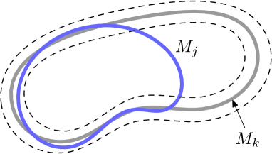
Figure 1. Illustration of the argument of Lemma 5.7 for $j>k$. The surface $M_{j}$ (blue) must leave the tubular neighbourhood (dashed line) around the surface $M_{k}$ (grey).

Proof.

As the statement is symmetric in $j$ and $k$, with no loss of generality we may assume that $j>k$. We proceed by contradiction and assume that for all $\delta>0$ there exist $V_{j}\in\mathcal{A}^{g}_{j}$ and $V_{k}\in\mathcal{A}_{k}^{g}$ with

$$W_{p}(V_{j},V_{k})<\delta^{2}.$$ (5.9)

We show that condition (5.9) leads to a contradiction if $\delta$ is chosen to be small enough. More precisely, we prove that one can find $0<\delta_{*}<1$ depending only on $k$ and $j$, as well as on the data $m_{0}$, $L$, and $p$, such that for any $0<\delta<\delta_{*}$ no varifolds $V_{j}\in\mathcal{A}^{g}_{j}$ and $V_{k}\in\mathcal{A}_{k}^{g}$ exist such that (5.9) holds.

Along the proof, we use the notation $V_{j}=V[M_{j},\tilde{\nu},j,0]$ and $V_{k}=V[M_{k},\nu,k,0]$ for any varifold in $\mathcal{A}^{g}_{j}$ and $\mathcal{A}_{k}^{g}$, respectively. Moreover, we indicate by $C_{i}>0$, $i=0,\dots,7$, some constants depending solely on the data, in particular possibly on $L$. To start with, let us note that there exists $C_{0}>0$ such that any $V\in\mathcal{A}^{g}$ is such that the corresponding spatial support $M$ in $\mathbb{R}^{3}$ fulfills the lower bound

$${\rm vol}(M)\geq C_{0},$$

where ${\rm vol}(M)$ indicates the volume of the region which is enclosed by $M$, cf. Subsection 4.2.1.

We subdivide the proof into three steps. At first, we show that any surface which is completely contained in a sufficiently small neighborhood of $M_{k}$ must have at least the area of $M_{k}$, up to a small error. Since

$$\mathcal{H}^{2}(M_{j})<\mathcal{H}^{2}(M_{k})$$

by $j>k$ and by the mass constraint, this implies that $M_{j}$ cannot be completely contained in such a small neighborhood of $M_{k}$, see Figure 1. In the second step, we give a lower bound on the area of $M_{j}$ which is not contained in the small neighborhood of $M_{k}$. Eventually, in Step 3 we show that such a lower bound contradicts condition (5.9).

Step 1: A lower bound on the area. We start by checking that one can find $\delta_{0}>0$ and $C_{1}>0$ such that

$$\forall\,0<\delta<\delta_{0},\ \forall\,V_{k}\in\mathcal{A}_{k}^{g},\ \forall\,E\subset\mathbb{R}^{3}\ \text{of finite perimeter with}\,\ |E|\geq C_{0}:$$

$$\quad\partial^{*}E\subset M_{k}^{\delta}:=M_{k}+B_{\delta}(0)\ \Rightarrow\ \mathcal{H}^{2}(\partial^{*}E)\geq\mathcal{H}^{2}(M_{k})-C_{1}\delta,$$ (5.10)

where we recall the notation for the open ball $B_{\delta}(0)=\{x\in\mathbb{R}^{3}:\>|x|<\delta\}$.

Let us start by choosing $\delta_{1}>0$ so small that the projection $\pi_{M_{k}}$ onto $M_{k}$ is well-defined on $M_{k}^{\delta_{1}}$, for any $V_{k}\in\mathcal{A}_{k}^{g}$. As $M_{k}$ is a set of positive reach, such a $\delta_{1}$ exists and depends on $L$ only. Then, one can find $C_{2}>0$ such that

$${\rm vol}(M_{k}^{\delta})\leq C_{2}\delta\mathcal{H}^{2}(M_{k})\quad\forall\,0<\delta<\delta_{1}.$$ (5.11)

Note that $C_{2}$ depends on $L$ and that the latter inequality cannot be guaranteed if the uniform $C^{1,1}$ regularity of $M_{k}$ is dropped. Next we choose $0<\delta_{0}<\min\{C_{0}k/(C_{2}m_{0}),\delta_{1}\}$, which implies that

$$\partial^{*}E\subset M_{k}^{\delta_{0}}\ \Rightarrow\ \pi_{M_{k}}(\partial^{*}E)\equiv M_{k}.$$

Indeed, if $\pi_{M_{k}}(\partial^{*}E)\not=M_{k}$, the fact that $\partial^{*}E\subset M_{k}^{\delta_{0}}$ would imply that the whole $E$ is contained in $M_{k}^{\delta_{0}}$. In combination with inequality (5.11) this would require that

$$C_{0}\leq|E|\leq{\rm vol}(M_{k}^{\delta_{0}})\leq C_{2}{\delta_{0}}\mathcal{H}^{2}(M_{k})=C_{2}{\delta_{0}}\frac{m_{0}}{k}<C_{0},$$

which is a contradiction.

Let $\xi\colon U\to\Sigma^{g}$ be a fixed smooth a.e. injective parametrization of $\Sigma^{g}\subset\mathbb{R}^{3}$ with $U=[0,1]^{2}$. We can cover $U$ up to a negligible set by the union of disjoint open sets $\{U_{i}\}_{i=1}^{N_{\eta}}$ on which $\xi$ is injective, each having diameter smaller than some given $\eta>0$, to be fixed below. Note that if $\eta$ is small enough, such a covering can be chosen in such a way that $N_{\eta}\leq 2/\eta^{2}$ (take disjoint open squares of side $\eta$, where we have $N_{\eta}\leq\lceil 1/\eta\rceil^{2}$, hence $N_{\eta}\leq 2/\eta^{2}$ for $0<\eta<(\sqrt{5}-1)/2\>$).

Given $V_{k}\in\mathcal{A}_{k}^{g}$ with $M_{k}=\psi(\Sigma^{g})$ as in (5.1), define $\phi:=\psi\circ\xi\colon U\to M_{k}$ and recall that the normal at $x\in M_{k}$ is indicated by $\nu(x)$. We let $u_{i}\in U_{i}$ be fixed and define $P_{i}\subset\mathbb{R}^{3}$ to be the tangent plane to $M_{k}$ at the point $x_{i}=\phi(u_{i})$. Moreover, for all $0<\delta<\delta_{0}$ we define the $\delta$-neighborhood of $\phi(U_{i})$ in the normal direction, namely,

$$D^{\delta}_{i}:=\{\tilde{x}=x+h\,\nu(x)\in\mathbb{R}^{3}:\>x\in\phi(U_{i}),\>|h|<\delta\},$$

see Figure 2.

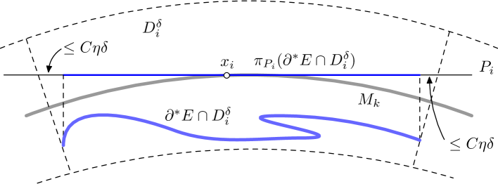
Figure 2. The notation of Step 1 in the proof of Lemma 5.7.

We observe that

$$\mathcal{H}^{2}(\partial^{*}E\cap D^{\delta}_{i})\geq\mathcal{H}^{2}(\pi_{P_{i}}(\partial^{*}E\cap D^{\delta}_{i})),$$ (5.12)

for orthogonal projections to a plane decrease the perimeter. Next, we bound $\mathcal{H}^{2}(\pi_{P_{i}}(\partial^{*}E\cap D^{\delta}_{i}))$ by the area of $P_{i}\cap D^{\delta}_{i}$, up to a small error. More precisely, we exploit the Lipschitz continuity of $x\mapsto\nu(x)$ in order to get that

$$\sup_{y\in P_{i}\cap D^{\delta}_{i}}\ \inf_{x\in\pi_{P_{i}}(\partial^{*}E\cap D^{\delta}_{i})}|x-y|\leq C_{3}\eta\delta,$$ (5.13)

where $C_{3}>0$ depends on $L$ only. By possibly choosing another constant $C_{4}>0$, again depending on $L$, we can check that the length of the boundary $\partial(P_{i}\cap D^{\delta}_{i})\subset P_{i}$ is bounded by $C_{4}\eta$. Inequality (5.13) hence implies that

$$\mathcal{H}^{2}(\pi_{P_{i}}(\partial^{*}E\cap D^{\delta}_{i}))\geq\mathcal{H}^{2}(P_{i}\cap D^{\delta}_{i})-C_{5}\eta^{2}\delta,$$ (5.14)

where $C_{5}>0$ is just depending on $L$. Eventually, one can estimate the area of $P_{i}\cap D^{\delta}_{i}$ via that of $\phi(U_{i})$. In fact, the surface $P_{i}\cap D^{\delta}_{i}$ can be parametrized over $U_{i}$ via

$$\tilde{\phi}(u)=\phi(u)+h(u)\nu(\phi(u))$$

where the $C^{1}$ function $h\colon U_{i}\to(-\delta,\delta)$ is uniquely determined by asking $P_{i}\cap D^{\delta}_{i}=\tilde{\phi}(U_{i})$. Owing to the smoothness of $M_{k}$ we can show that the infinitesimal area elements on $\phi(U_{i})$ and $P_{i}\cap D^{\delta}_{i}$ are comparable. For this purpose, we introduce the short-hand notation

$$a:=\partial_{1}\phi\times\partial_{2}\phi\colon U_{i}\to\mathbb{R}^{3}\quad\text{and}\quad\tilde{a}:=\partial_{1}\tilde{\phi}\times\partial_{2}\tilde{\phi}\colon U_{i}\to\mathbb{R}^{3}.$$

As by definition $\tilde{a}=(\partial_{1}\phi+(\partial_{1}h)\nu+h(\nabla\nu)\partial_{1}\phi)\times(\partial_{2}\phi+(\partial_{2}h)\nu+h(\nabla\nu)\partial_{2}\phi)$, we get

$$a\cdot\tilde{a}=|a|^{2}+b\cdot a$$

for $b:=\partial_{1}\phi\times h(\nabla\nu)\partial_{2}\phi+h(\nabla\nu)\partial_{1}\phi\times\partial_{2}\phi+h^{2}(\nabla\nu)\partial_{1}\phi\times(\nabla\nu)\partial_{2}\phi$. We can hence find $C_{6}>0$ such that $|\tilde{a}|\leq C_{6}$ and $|b|\leq C_{6}\delta$. As $x\mapsto\frac{a(x)}{|a(x)|}=\nu(x)$ is Lipschitz continuous we get $|\frac{a}{|a|}-\frac{\tilde{a}}{|\tilde{a}|}|\leq C_{7}\eta.$ The latter in particular entails that

$$C_{7}\eta\geq\left|\left(\frac{a}{|a|}-\frac{\tilde{a}}{|\tilde{a}|}\right)\cdot\frac{\tilde{a}}{|\tilde{a}|}\right|=\left|\frac{a\cdot\tilde{a}}{|a|\,|\tilde{a}|}-1\right|=\left|\frac{|a|^{2}+b\cdot a}{|a|\,|\tilde{a}|}-1\right|.$$

By multiplying by $|\tilde{a}|$ we obtain $\left||a|-|\tilde{a}|+\frac{b\cdot a}{|a|}\right|\leq C_{7}\eta|\tilde{a}|.$ Eventually, by using the bounds $|\tilde{a}|\leq C_{6}$ and $|b|\leq C_{6}\delta$, we conclude that

$$\big{|}|\partial_{1}\phi\times\partial_{2}\phi|-|\partial_{1}\tilde{\phi}\times\partial_{2}\tilde{\phi}|\big{|}\leq C_{6}\delta+C_{6}C_{7}\eta.$$

This implies

$$\mathcal{H}^{2}(P_{i}\cap D^{\delta}_{i}) =\int_{U_{i}}|\partial_{1}\tilde{\phi}\times\partial_{2}\tilde{\phi}|\geq\int_{U_{i}}\big{(}|\partial_{1}\phi\times\partial_{2}\phi|-(C_{6}\delta+C_{6}C_{7}\eta)\big{)}$$

$$=\mathcal{H}^{2}(\phi(U_{i}))-(C_{6}\delta+C_{6}C_{7}\eta)\mathcal{H}^{2}(U_{i}).$$ (5.15)

By combining inequalities (5.12), (5.14)-(5.15), and summing for $i=1,\dots,N_{\eta}$, we get

$$\mathcal{H}^{2}(\partial^{*}E) \geq\mathcal{H}^{2}(M_{k})-C_{5}\eta^{2}\delta N_{\eta}-(C_{6}\delta+C_{6}C_{7}\eta)\mathcal{H}^{2}(U)$$

$$\geq\mathcal{H}^{2}(M_{k})-2C_{5}\delta-(C_{6}\delta+C_{6}C_{7}\eta).$$

It hence suffices to let $\eta=\delta$ and define $C_{1}:=2C_{5}+C_{6}+C_{6}C_{7}$ to obtain (5.10).

Step 2: Uniform bound of the excess area. Given $V_{j}\in\mathcal{A}^{g}_{j}$, we apply (5.10) to $E\subset\mathbb{R}^{3}$ with $\partial E=M_{j}$. Consequently, if $M_{j}\subset M_{k}^{\delta}$, then

$$\frac{m_{0}}{j}=\mathcal{H}^{2}(M_{j})\geq\mathcal{H}^{2}(M_{k})-C_{1}\delta>\frac{m_{0}}{k}-C_{1}\delta_{0}$$

is true for any $0<\delta<\delta_{0}$. Recalling $j>k$, this leads to a contradiction as soon as

$$C_{1}\delta_{0}<\frac{m_{0}}{k}-\frac{m_{0}}{j}.$$ (5.16)

Under the latter assumption, we have hence proved that $M_{j}\not\subset M_{k}^{\delta}$ for any $\delta<\delta_{0}$ and any $V_{j}\in\mathcal{A}^{g}_{j}$ and $V_{k}\in\mathcal{A}_{k}^{g}$.

We now aim at refining this argument by showing that, for $\delta$ small enough, the area of the portion of $M_{j}$ which is not contained in $M_{k}^{\delta}$ can be uniformly bounded from below. More precisely, given any bounded open set $A\subset\mathbb{R}^{3}$, we show that there exists $0<\delta_{*}<\delta_{0}$ such that

$$\forall\,V_{k}\in\mathcal{A}_{k}^{g},\,\forall\,E\subset\mathbb{R}^{3}\ \text{with}\ {\rm Per}(E;A)\leq\frac{m_{0}}{j},\ |E|\geq C_{0}:\quad{\rm Per}(E;(\overline{M_{k}^{\delta_{*}}})^{c})\geq\delta_{*}.$$ (5.17)

Statement (5.17) can be checked by contradiction: assume that for all $0<\delta<\delta_{0}$ there exists $E_{\delta}\subset\mathbb{R}^{3}$ with ${\rm Per}(E_{\delta};A)\leq m_{0}/j$, $|E_{\delta}|\geq C_{0}$, and ${\rm Per}(E_{\delta};(\overline{M_{k}^{\delta}})^{c})<\delta$. By compactness in the class of finite-perimeter sets we find a not relabeled subsequence $(E_{\delta})_{\delta}$ and a finite perimeter set $E\subset\mathbb{R}^{3}$ such that, as $\delta\to 0$, the characteristic functions $1_{E_{\delta}}$ converge to $1_{E}$ in $L^{1}(\mathbb{R}^{3})$ and the Radon measures $\mu_{\delta}:=-\mathrm{D}1_{E_{\delta}}$ fulfill $\mu_{\delta}\rightharpoonup^{\ast}\mu=-\mathrm{D}1_{E}$. This implies that ${\rm vol}(E)\geq C_{0}$ and ${\rm Per}(E;A)\leq m_{0}/j$, as well. Moreover, for all $0<\overline{\delta}<\delta_{0}$ we have that

$${\rm Per}(E;(\overline{M_{k}^{\overline{\delta}}})^{c})\leq\liminf_{\delta\to 0}{\rm Per}(E_{\delta};(\overline{M_{k}^{\overline{\delta}}})^{c})\leq\liminf_{\delta\to 0}{\rm Per}(E_{\delta};(\overline{M_{k}^{\delta}})^{c})=0.$$

This shows that $\partial^{*}E\subset M_{k}^{\overline{\delta}}$. By applying estimate (5.10) we deduce that ${\rm Per}(E;M^{\delta_{1}}_{k})\geq\mathcal{H}^{2}(M_{k})-C_{1}\overline{\delta}$ which leads to a contradiction as

$$\frac{m_{0}}{j}\geq{\rm Per}(E;M^{\delta_{1}}_{k})\geq\mathcal{H}^{2}(M_{k})-C_{1}\overline{\delta}=\frac{m_{0}}{k}-C_{1}\overline{\delta}\stackrel{{\scriptstyle\eqref{eq:deltamo}}}{{>}}\frac{m_{0}}{j}.$$

This proves that there exists $0<\delta_{*}<\delta_{1}$ such that (5.17) holds. In particular, for all $V_{j}\in\mathcal{A}^{g}_{j}$ and $V_{k}\in\mathcal{A}_{k}^{g}$ we have that

$$\mathcal{H}^{2}(M_{j}\cap(\overline{M_{k}^{\delta_{*}}})^{c})\geq\delta_{*}.$$ (5.18)

Step 3: Conclusion of the proof. Let $V_{j}\in\mathcal{A}^{g}_{j}$ and $V_{k}\in\mathcal{A}_{k}^{g}$ fulfill condition (5.9) for some $\delta<\delta_{*}$. Denote by $\lambda\in\Pi(V_{k},V_{j})\subset\mathcal{M}((\mathbb{R}^{3}\times\SS^{2})^{2})$ an optimal transport plan between $V_{k}$ and $V_{j}$, i.e.,

$$W_{p}^{p}(V_{j},V_{k})=\int_{(\mathbb{R}^{3}\times\SS^{2})^{2}}d^{p}((x,\nu),(\tilde{x},\tilde{\nu}))\,\,\mathrm{d}\lambda((x,\nu),(\tilde{x},\tilde{\nu})),$$

where we recall that $d((x,\nu),(\tilde{x},\tilde{\nu}))=|x-\tilde{x}|+|\nu-\tilde{\nu}|$. Consider the ${\delta}$-neighborhood $N^{\delta}$ of the diagonal in $(\mathbb{R}^{3}\times\SS^{2})^{2}$ given by

$$N^{\delta}:=\left\{(y,\tilde{y})\in(\mathbb{R}^{3}\times\SS^{2})^{2}:\>d(y,\tilde{y})<{\delta}\right\}.$$

As $1\leq\delta^{-p}d^{p}(y,\tilde{y})$ for all $(y,\tilde{y})\in(N^{\delta})^{c}$ we can estimate the measure of the complement $(N^{\delta})^{c}$ by a classical Chebyshev-type argument:

$$\lambda((N^{\delta})^{c})=\int_{(N^{\delta})^{c}}\,\mathrm{d}\lambda\leq\delta^{-p}\int_{(\mathbb{R}^{3}\times\SS^{2})^{2}}d^{p}(y,\tilde{y})\,\mathrm{d}\lambda(\tilde{y},y)=\delta^{-p}W_{p}^{p}(V_{j},V_{k})\stackrel{{\scriptstyle\eqref{eq:condition}}}{{<}}\delta^{p}.$$ (5.19)

Next we observe that $\tilde{x}\in M_{j}\cap(\overline{M_{k}^{\delta}})^{c}$ implies $|\tilde{x}-x|\geq{\delta}$ and thus $((x,\nu(x)),(\tilde{x},\tilde{\nu}(\tilde{x})))\in(N^{\delta})^{c}$ for all $x\in M_{k}$. With $Z:=\{((x,\nu(x)),(\tilde{x},\tilde{\nu}(\tilde{x})))\in(\mathbb{R}^{3}\times\SS^{2})^{2}:\>x\in M_{k},\,\tilde{x}\in M_{j}\cap(\overline{M_{k}^{\delta}})^{c}\}\subset(N^{\delta})^{c}$ we hence have that

$$\mathcal{H}^{2}(M_{j}\cap(\overline{M_{k}^{\delta}})^{c})\leq\lambda(Z)\leq\lambda((N^{\delta})^{c})\stackrel{{\scriptstyle\eqref{eq:Cheby}}}{{<}}\delta^{p}.$$ (5.20)

Eventually, we combine inequalities (5.18) and (5.20) to get

$$\delta>\delta^{p}\stackrel{{\scriptstyle\eqref{eq:step3}}}{{>}}\mathcal{H}^{2}(M_{j}\cap(\overline{M_{k}^{\delta}})^{c})\geq\mathcal{H}^{2}(M_{j}\cap(\overline{M_{k}^{\delta_{*}}})^{c})\stackrel{{\scriptstyle\eqref{eq:step2}}}{{\geq}}\delta_{*}>\delta$$

which is a contradiction. ∎

5.6. Existence of GMMs under a weaker metric

In the regular case, one can prove the existence of GMMs for the Canham-Helfrich functional under the weaker metric given by the Wasserstein distance of the spatial supports. Indeed, let $V^{0},V^{1}\in\mathcal{P}(\mathbb{R}^{3}\times\SS^{2})$ and set $\mu^{0}:=\mu_{V^{0}},\mu^{1}:=\mu_{V^{1}}\in\mathcal{P}(\mathbb{R}^{3})$. Then, one can prove that the varifold Wasserstein distance, $W_{p}(V^{1},V^{0})$, controls the Wasserstein distance between spatial Radon measures, $\overline{W}_{p}(\mu^{1},\mu^{0})$, in the following sense

$$W_{p}(V^{1},V^{0})\geq\overline{W}_{p}(\mu^{1},\mu^{0}).$$

Indeed, with $\lambda\in\Pi(V^{1},V^{0})$ realizing the minimum in the definition of $W_{p}(V^{1},V^{0})$, we get

$$W_{p}^{p}(V^{1},V^{0})=\int_{(\mathbb{R}^{3}\times\SS^{2})^{2}}(|x-\tilde{x}|+|\nu-\tilde{\nu}|)^{p}\,\mathrm{d}\lambda((x,\nu),(\tilde{x},\tilde{\nu}))$$

$$=\int_{(\mathbb{R}^{3}\times\SS^{2})^{2}}|x-\tilde{x}|^{p}\,\mathrm{d}\lambda((x,\nu),(\tilde{x},\tilde{\nu}))+\underbrace{\sum_{k=1}^{p}\binom{p}{k}\int_{(\mathbb{R}^{3}\times\SS^{2})^{2}}|x-\tilde{x}|^{p-k}|\nu-\tilde{\nu}|^{k}\,\mathrm{d}\lambda((x,\nu),(\tilde{x},\tilde{\nu}))}_{\geq\>0}$$

$$\geq\int_{\mathbb{R}^{3}\times\mathbb{R}^{3}}|x-\tilde{x}|^{p}\,\mathrm{d}(\pi_{\sharp}^{\mathbb{R}^{3}}\lambda)(x,\tilde{x})\underbrace{\int_{\SS^{2}\times\SS^{2}}\,\mathrm{d}(\pi_{\sharp}^{\SS^{2}}\lambda)(\nu,\tilde{\nu})}_{=\>1}\geq\overline{W}_{p}^{p}(\mu^{1},\mu^{0}),$$

as the $\mathbb{R}^{3}\times\SS^{2}$-marginals $V^{0}$ and $V^{1}$ of $\lambda$ are oriented varifolds of the form (3.9) and the $(\mathbb{R}^{3})^{2}$-marginal $\pi_{\sharp}^{\mathbb{R}^{3}}\lambda\in\mathcal{M}((\mathbb{R}^{3})^{2})$ is a possible choice in $\Pi(\mu^{1},\mu^{0})$.

On the other hand, as soon as multiplicity is fixed to some $k\in\mathbb{N}$ and we restrict to the regular varifolds $V^{1},V^{0}\in\mathcal{A}_{k}^{g}$ (5.1), which have with fixed orientation, we have that

$$\overline{W}_{p}(\mu^{1},\mu^{0})=0\>\Longrightarrow\>W_{p}(V^{1},V^{0})=0,$$ (5.21)

for $\overline{W}_{p}(\mu^{1},\mu^{0})=0$ in particular implies that $M^{0}=M^{1}=:M$. The equality $V^{1}=V^{0}$ then follows from $V^{0}=V[M,\nu^{M},k,0]=V^{1}$ with $\mu_{V^{0}}=k(\mathcal{H}^{2}\,\text{\Large{\reflectbox{$\lrcorner$}}}M)$.

The nondegeneracy condition (5.21) is instrumental in proving the existence of GMMs, because it qualifies $\overline{W}_{p}$ as a distance on $\mathcal{A}_{k}^{g}$. Correspondingly, the existence result from [3, Prop. 2.2.3] can still be applied. However, note that condition (5.21) hinges on the conservation of multiplicity and that the proof of Theorem 5.6, in particular the argument of Lemma 5.7, requires the control of the stronger distance $W_{p}(V^{1},V^{0})$. This amounts to say that, effectively, we can resort to the weaker metric $\overline{W}_{p}(\mu^{1},\mu^{0})$ just in the frame of GMMs restricted a priori to $\mathcal{A}^{g}$, namely, multiply covered uniformly regular $C^{1,1}$ surfaces.

5.7. More general curvature functionals

Most results of this section can also be established for a larger class of geometric functionals. In particular, we could prove the existence of GMMs for more general curvature energies of the form

$$D(M):=\int_{M}f(x,\nu(x),H(x),K(x))\,\mathrm{d}\mathcal{H}^{2}(x).$$

Here, $M$ is a uniformly regular $C^{1,1}$ surface in $\mathbb{R}^{3}$, as in (5.1), and the integrand $f$ is continuous and convex in its last two arguments. This class of curvature functionals has already been considered in [25] concerning equilibrium problems. In particular, it has been verified there that $D$ admits minimizers in $\mathcal{A}^{g}_{1}$ for any fixed genus $g\in\mathbb{N}$, also under a volume constraint.

The analysis in [25] hinges upon the compactness of $\mathcal{A}^{g}_{1}$ and on the lower semicontinuity of $D$. These same tools ensure the existence of a GMM for $D$ with respect to the Wasserstein metric $W_{p}$. The adjustments required are mainly notational. The only point deserving some attention is the a priori multiplicity bound in terms of the functional, for a Li-Yau inequality may fail in degenerate cases. Still, a bound on the multiplicity can be directly deduced from the uniform $C^{1,1}$ regularity, i.e., depending on the constant $L$ in the definition (5.1) of $\mathcal{A}^{g}_{k}$. By assuming such a priori bound on the multiplicity, the argument of Theorem 5.6 still holds. In particular, multiplicity is conserved along the evolution. Moreover, in the weaker metric setting given by the Wasserstein distance $\overline{W}_{p}$ on the spatial supports, one can still prove existence of a restricted GMM to $\mathcal{A}^{g}_{k}$ by constraining the multiplicity.

References

- [1] W. K. Allard. On the first variation of a varifold. Ann. of Math. (2), 95:417–491, 1972.
- [2] L. Ambrosio. Minimizing movements. Rend. Accad. Naz. Sci. XL Mem. Mat. Appl. (5), 19:191–246, 1995.
- [3] L. Ambrosio, N. Gigli, and G. Savaré. Gradient flows in metric spaces and in the space of probability measures. Second edition. Birkhäuser Verlag, Basel, 2008.
- [4] J. W. Barrett, H. Garcke, and R. Nürnberg. Parametric approximation of Willmore flow and related geometric evolution equations. SIAM J. Sci. Comput. 31(1):225–-253, 2008.
- [5] J. W. Barrett, H. Garcke, and R. Nürnberg. Computational parametric Willmore flow with spontaneous curvature and area difference elasticity effects. SIAM J. Numer. Anal. 54(3):1732–1762, 2016.
- [6] J. W. Barrett, H. Garcke, and R. Nürnberg. Finite element approximation for the dynamics of fluidic two-phase biomembranes. ESAIM Math. Model. Numer. Anal. 51(6):2319–2366, 2017.
- [7] J. W. Barrett, H. Garcke, and R. Nürnberg. Gradient flow dynamics of two-phase biomembranes: Sharp interface variational formulation and finite element approximation. SMAI J. Comput. Math. 4:151–195, 2018.
- [8] S. Blatt. A singular example for the Willmore flow. Analysis (Munich) 29(4):407–-430, 2009.
- [9] S. Blatt. A note on singularities in finite time for the gradient flow of the Helfrich functional. J. Evol. Equ. 19(2):463-–477, 2019.
- [10] V. Bogachev. Measure theory. Vol. II. Springer-Verlag, Berlin, 2007.
- [11] K. Brazda, L. Lussardi, and U. Stefanelli. Existence of varifold minimizers for the multiphase Canham-Helfrich functional. Calc. Var. Partial Differential Equations, 59(3):93, 26 pp., 2020.
- [12] B. Buet, G.P. Leonardi, and S. Masnou. A varifold approach to surface approximation. Arch. Ration. Mech. Anal. 226(2):639–694, 2017.
- [13] B. Buet, G.P. Leonardi, and S. Masnou. Weak and approximate curvatures of a measure: A varifold perspective, Nonlinear Anal., 222:112983, 2022.
- [14] P. B. Canham. The minimum energy of bending as a possible explanation of the biconcave shape of the human red blood cell. J. Theor. Biol. 26:61–80, 1970.
- [15] R. Choksi and M. Veneroni. Global minimizers for the doubly-constrained Helfrich energy: The axisymmetric case. Calc. Var. Partial Differential Equations, 48 (3-4):337–366, 2013.
- [16] R. Choksi, M. Morandotti, and M. Veneroni. Global minimizers for axisymmetric multiphase membranes. ESAIM Control Optim. Calc. Var. 19(4):1014–1029, 2013.
- [17] P. Colli, Pierluigi and P. Laurençot. A phase-field approximation of the Willmore flow with volume and area constraints. SIAM J. Math. Anal. 44(6), 3734-–3754, 2012.
- [18] E. De Giorgi. New problems on minimizing movements, In: Boundary Value Problems for Partial Differential Equations and Applications, RMA Res. Notes Appl. Math. 29:81–98, Masson, Paris, 1993.
- [19] S. Eichmann. Lower-semicontinuity for the Helfrich problem. Ann. Global Anal. Geom. 58(2):147–175, 2020.
- [20] C. M. Elliott and B. Stinner. Modeling and computation of two phase geometric biomembranes using surface finite elements. J. Comput. Phys. 229(18):6585–-6612, 2010.
- [21] C. M. Elliott and L. Hatcher. Domain formation via phase separation for spherical biomembranes with small deformations. European J. Appl. Math. 32(6):1127–-1152, 2021.
- [22] M. Fei and Y. Liu. Phase-field approximation of the Willmore flow. Arch. Ration. Mech. Anal. 241(3)1655–-1706, 2021.
- [23] A. Dall’Acqua, M. Müller, R. Schätzle, A. Spener. The Willmore flow of tori of revolution. arXiv:2005.13500, 2020.
- [24] J. Dalphin. Etude de fonctionnelles géométriques dépendant de la courbure par des méthodes d’optimisation de formes. Applications aux fonctionnelles de Willmore et Canham-Helfrich. PhD Thesis, 2014.
- [25] J. Dalphin. Uniform ball property and existence of optimal shapes for a wide class of geometric functionals. Interfaces Free Bound. 20:211–260, 2018.
- [26] H. Federer. Curvature measures. Trans. Amer. Math. Soc. 93(3):418–491, 1959.
- [27] H. Federer. Geometric measure theory. Springer, New York, 1969.
- [28] H. Garcke, and R. Nürnberg. Structure-preserving discretizations of gradient flows for axisymmetric two-phase biomembranes. IMA J. Numer. Anal. 41(3):1899-–1940, 2021.
- [29] W. Helfrich. Elastic properties of lipid bilayers: Theory and possible experiments. Z. Naturforsc. C, 28(11–12):693–703, 1973.
- [30] J. E. Hutchinson. Second fundamental form for varifolds and the existence of surfaces minimising curvature. Indiana Univ. Math. J. 35(1):45–71, 1986.
- [31] M. Köhne and D. Lengeler. Local well-posedness for relaxational fluid vesicle dynamics. J. Evol. Equ. 18(4):1787-–1818, 2018.
- [32] Y. Kohsaka and T. Nagasawa. On the existence of solutions of the Helfrich flow and its center manifold near spheres. Differential Integral Equations 19(2):121–142, 2006.
- [33] A. Kubin, L. Lussardi and M. Morandotti. Direct minimization of the Canham–Helfrich energy on generalized Gauss graphs. arXiv:2201.06353, 2022.
- [34] J. LeCrone, Y. Shao, and G. Simonett. The surface diffusion and the Willmore flow for uniformly regular hypersurfaces. Discrete Contin. Dyn. Syst. Ser. S 13(12):3503–-3524, 2020.
- [35] P. Li and S. T. Yau. A new conformal invariant and its applications to the Willmore conjecture and the first eigenvalue of compact surfaces. Invent. Math. 69(2), 269–291, 1982.
- [36] E. Kuwert and R. Schätzle. The Willmore flow with small initial energy. J. Differential Geom. 57(3):409–441, 2001
- [37] E. Kuwert and R. Schätzle. Gradient flow for the Willmore functional. Comm. Anal. Geom. 10(2):307–-339, 2002.
- [38] E. Kuwert and R. Schätzle. Removability of point singularities of Willmore surfaces. Ann. of Math. (2), 160:315–357, 2004.
- [39] E. Kuwert and R. Schätzle. The Willmore functional. In: Topics in modern regularity theory, CRM Series 13:1–115, Ed. Norm., Pisa, 2012.
- [40] E. Kuwert, J. Scheuer. Asymptotic estimates for the Willmore flow with small energy. Int. Math. Res. Not. IMRN, 18:14252–14266, 2021.
- [41] D. Lengeler. Asymptotic stability of local Helfrich minimizers. Interfaces Free Bound. 20(4):533–-550, 2018.
- [42] Y. Liu. Gradient flow for the Helfrich functional. Chinese Ann. Math. Ser. B 33(6):931-–940, 2012.
- [43] C. Mantegazza. Curvature varifolds with boundary. J. Differential Geom. 43(4):807–843, 1996.
- [44] J. McCoy and G. Wheeler. Finite time singularities for the locally constrained Willmore flow of surfaces. Comm. Anal. Geom. 24(4):843–-886, 2016.
- [45] A. Mondino and C. Scharrer. Existence and regularity of spheres minimising the Canham-Helfrich energy. Arch. Ration. Mech. Anal. 236(3):1455–1485, 2020.
- [46] T. Nagasawa and T. Yi. Local existence and uniqueness for the -dimensional Helfrich flow as a projected gradient flow. Hokkaido Math. J. 41(2):209-–226, 2012.
- [47] F. Palmurella and T. Rivière. The parametric approach to the Willmore flow. Adv. Math. 400, Paper No. 108257, 48 pp., 2022.
- [48] A. Rätz and M. Röger. A new diffuse-interface approximation of the Willmore flow. ESAIM Control Optim. Calc. Var. 27(14), 28 pp., 2021.
- [49] J. Rataj and M. Zaehle. Curvature Measures of Singular Sets. Springer, 2019.
- [50] F. Rupp. The volume-preserving Willmore flow. arXiv.2012.03553, 2020.
- [51] F. Rupp. The Willmore flow with prescribed isoperimetric ratio. arXiv.2106.02579, 2021.
- [52] F. Rupp and C. Scharrer. Li-Yau inequalities for the Helfrich functional and applications. arXiv.2203.12360, 2022.
- [53] L. Simon. Lectures on geometric measure theory. vol. 3 of Proceedings of the Centre for Mathematical Analysis. Australian National University, Canberra, 1983 (reprinted 2014).
- [54] L. Simon. Existence of surfaces minimizing the Willmore functional. Comm. Anal. Geom. 1(2):281–326, 1993.
- [55] G. Simonett. The Willmore flow near spheres. Differential Integral Equations, 14(8):1005–1014, 2001.
- [56] P. Topping. Mean curvature flow and geometric inequalities. J. Reine Angew. Math. 503:47–61, 1998.
- [57] T. J. Willmore, Riemannian Geometry, Oxford University Press, 1996.
- [58] W. Wang, P. Zhang, and Z. Zhang. Well-posedness of hydrodynamics on the moving elastic surface. Arch. Ration. Mech. Anal. 206(3):953–995, 2012.