Batch Evaluation Metrics in Information Retrieval:
Measures, Scales, and Meaning

Abstract

A sequence of recent papers has considered the role of measurement scales in information retrieval (IR) experimentation, and presented the argument that (only) uniform-step interval scales should be used, and hence that well-known metrics such as reciprocal rank, expected reciprocal rank, normalized discounted cumulative gain, and average precision, should be either discarded as measurement tools, or adapted so that their metric values lie at uniformly-spaced points on the number line. These papers paint a rather bleak picture of past decades of IR evaluation, at odds with the community’s overall emphasis on practical experimentation and measurable improvement.

Our purpose in this work is to challenge that position. In particular, we argue that mappings from categorical and ordinal data to sets of points on the number line are valid provided there is an external reason for each target point to have been selected. We first consider the general role of measurement scales, and of categorical, ordinal, interval, ratio, and absolute data collections. In connection with the first two of those categories we also provide examples of the knowledge that is captured and represented by numeric mappings to the real number line. Focusing then on information retrieval, we argue that document rankings are categorical data, and that the role of an effectiveness metric is to provide a single value that represents the usefulness to a user or population of users of any given ranking, with usefulness able to be represented as a continuous variable on a ratio scale. That is, we argue that current IR metrics are well-founded, and, moreover, that those metrics are more meaningful in their current form than in the proposed “intervalized” versions.

1 Introduction

We use measurement to capture data about some attribute or observation of a real-world phenomenon. For example, a thermometer measures temperature so that we have guidance as to how hot or cold we might feel if we went outdoors; and weather forecasts and climate summaries predict temperatures based on datasets of past observations so that we can make informed choices about our future activities. All other things being equal, a beach-side holiday at a location with an average daytime temperature of $25{}^{\circ}$C is likely to be preferable to one at a location with an average daytime temperature of $10{}^{\circ}$C.

If a measurement is to be useful, it should be connected to the attribute it refers to, and allow inferences to be derived from sets of measurements that are both predictive of, and connected to, the reality that is being measured. The extent to which inferences can be derived from measurements is, in part, determined by the scale that is employed, defined as the way in which observed attributes are represented by measured surrogates. For example, patients in a hospital may be asked to rate their pain on a scale of one to ten, with “perceived patient pain” the attribute, and a set of ten ordered categories as the corresponding measurement. Pain amelioration medications might then in part be selected in accordance with the measurement a patient reports, even though patients are not calibrated “pain-o-meters”.

Stevens (1946) described four scales of measurement, and enumerated their permissible operations in terms of what can be legitimately concluded about the behavior of the underlying attribute, given knowledge of the measurement, or of a set of measurements. In the case of a “ten point” pain assessment, for example, if yesterday a patient said “eight” and today they say “four”, we can be confident that their perceived pain has decreased, but should not say that it has halved – the conclusion “has decreased” is permissible, but the conclusion “has halved” is not, and nor is the conclusion “has gone down by four”. In the case of ordinal measures (which is what the ten point pain scale is), comparison of measurements is permitted as a valid reflection of the relative values of the corresponding underlying attributes, but the taking of ratios and differences is not (at least, not necessarily). Indeed, a patient’s subjective pain scale might be highly non-linear. Section 2 provides more detail of Stevens’ hierarchy of scales of measurement.

In a sequence of recent papers, Ferrante et al. (2019, 2020, 2021) have explored the way in which experimental measurement is carried out in information retrieval (IR), with particular emphasis on the use of interval scales, one of Stevens’ four scale categories. In a somewhat bleak assessment, Ferrante et al. conclude that IR has, by and large, employed inappropriate measurement scales for the last several decades, and (at risk of putting words into their mouths) that the discipline now has an opportunity to lift its game. In their most recent contribution, Ferrante et al. (2021) propose that each existing IR metric be “intervalized” in order to be rendered sound, with raw metric values mapped to evenly distributed points on the number line, the goal being to create a corresponding adjusted metric on equi-interval measurement scale.

Our goal here is to express a more optimistic view of IR evaluation and IR measurement, and to challenge the conclusions of Ferrante et al. We argue that the majority of existing IR metrics are in fact well-founded in terms of measurement and, for the most part, achieve what it was that they were designed to capture. We also differ from Ferrante et al. in regard to the worth of “intervalization” as a corrective mechanism.

In Section 2 Stevens’ measurement scale typology is explained, and examples of categorical, ordinal, and interval scales are provided. Section 3 then focuses in IR evaluation, and explains how IR measures are defined; assesses them against Stevens’ hierarchy; summarizes Ferrante et al.’s proposals; and explains why we diverge from them. Section 4 then considers other related work, and other aspects of IR experimental methodology that researchers and practitioners alike should bear in mind.

2 Background

The distinction between categorical, ordinal, interval, and ratio measures was introduced by Stevens (1946) and is now widely summarized in textbooks and online resources. This section provides an overview of those four classes, starting with categorical and ordinal measures, and examples thereof; then taking a diversion into a parable in which professors’ salaries are tabulated; and finishing with a description of interval and ratio measures. Section 3 then considers the ways in which measures are applied to evaluation in information retrieval.

2.1 Categorical Data

Table 1: Two sets of categorical (or nominal) labels: (a) the standard set of country codes, used perhaps to record country of birth in personnel data; and (b) a set of academic work categories at a university.

Label	Class
AU	Australia
CL	Chile
CN	China
IT	Italy
JP	Japan
(a) Countries of birth
Label	Class
AM	administrative and management
RO	research focused
TO	teaching focused
TR	teaching and research
(b) Academic employment types in a university

In a categorical (or nominal) measure each object in the data collection of interest (a dataset) is assigned to a single class, with the classes identified via a set of class labels. Table 1 provides two examples. In Table 1(a) the classes are countries, perhaps reflecting birth locations of university employees, and the class labels are two letter acronyms; and in Table 1(b) the classes are academic work categories in a university, and the labels are again two letter acronyms. For example, the birth countries of a group of ten professors at a university might be represented by the dataset:

$$\{\mbox{\sf{AU}},\mbox{\sf{CN}},\mbox{\sf{AU}},\mbox{\sf{IT}},\mbox{\sf{CL}},\mbox{\sf{CL}},\mbox{\sf{CN}},\mbox{\sf{AU}},\mbox{\sf{IT}},\mbox{\sf{JP}}\}\,.$$

The cardinality of each class across the dataset can be tabulated and used to summarize fractions (and hence allow representation as pie charts, including pie charts in which the segments are ordered from largest to smallest), and the mode (most frequent class) can be reported, as can other class ranks based on frequency of occurrence. For example, in the example dataset, the most common birth country is AU, accounting for $3/10$ of the professors; similarly (in the context of Table 1(b)), a university might report that “research focused” RO staff are its second largest category, accounting for $31$% of its employees.

In categorical data there is no meaningful ordering between the classes, and the only operations that can be applied to data items are equality and inequality testing ($=$ and $\not=$). The classes themselves can be ordered by considering their labels to be ASCII strings, as has been done in the two table sections, but that is purely for presentational convenience, and not an intrinsic feature of the data. If the class labels changed (or even if they didn’t) the table rows could be reordered, without affecting the validity or accuracy of any conclusions drawn from the dataset being discussed.

This absence of ordering between the classes means that the median (and other percentiles), and arithmetic and geometric averages, are meaningless concepts – a fact immediately grasped when considering the questions “average country of birth” and “median work category” of the ten professors mentioned above. Moreover, the inappropriateness of computing medians and means remains even if the class labels “look” like numbers. For example, suppose that the international phone dialing prefixes were used as the class labels, rather than the two letter acronyms: +61 for Australia, +56 for Chile, and so on (let’s ignore the fact that +1 actually covers several countries). The same dataset of ten professors would now be described as:

$$\{\mbox{\sf{+61}},\mbox{\sf{+86}},\mbox{\sf{+61}},\mbox{\sf{+39}},\mbox{\sf{+56}},\mbox{\sf{+56}},\mbox{\sf{+86}},\mbox{\sf{+61}},\mbox{\sf{+39}},\mbox{\sf{+81}}\}\,,$$

but it is still not permissible to compute the median or mean.

When categorical data is combined into ordered tuples – for example, the pairing “$\langle$country of birth, work category$\rangle$” – the set of tuples is also categorical data.

Table 2: Four sets of ordinal labels, and for each set, one possible mapping between the set’s categories and the real number line: (a) the set of available options (radio buttons) in a survey about frequency of alcohol consumption, with $N(\cdot)$ in “risk points”; (b) the set of professorial ranks at some university, with $N(\cdot)$ in “salary, dollars per week”; (c) the set of summative recommendations (radio buttons) available to referees during a peer review process, with $N(\cdot)$ a numeric mapping; and (d) the set of relevance labels employed in a document judging process as part of an IR evaluation, with $N(\cdot)$ a gain expressed in units of “utility”.

Label	Class	$N(\cdot)$
A0	never	$0$
A1	monthly or less	$1$
A2	two to four times a month	$2$
A3	two to three times a week	$3$
A4	four or more times per week	$4$
(a) Screening for alcohol consumption (one question of several)
Source: https://www.uptodate.com/contents/calculator-alcohol-consumption-screening-
audit-questionnaire-in-adults-patient-education
Label	Class	$N(\cdot)$
P1	junior professor	$\$700$
P2	assistant professor	$\$750$
P3	associate professor	$\$850$
P4	full professor	$\$1000$
(b) Professorial ranks
Label	Class	$N(\cdot)$
SR	strong reject	$-3$
R	reject	$-2$
WR	weak reject	$-1$
WA	weak accept	$+1$
A	accept	$+2$
SA	strong accept	$+3$
(c) Referee evaluations during peer review
Label	Class	$N(\cdot)$
G0	not relevant	$0.00$
G1	somewhat relevant	$0.25$
G2	relevant	$0.75$
G3	highly relevant	$1.00$
(d) Grades for document relevance to a topic

2.2 Ordinal Data

Ordinal data classes result if strict inequality as well as equality are permissible operators for comparing data items, that is, if all of $=$, $\not=$, $<$, and $>$ are operational. Table 2 gives four instances of ordinal class labels and class descriptions; the final column headed $N(\cdot)$ will be discussed shortly. The first section of Table 2 is taken from an online “alcohol risk screening” assessment, and is one of a suite of questions that collectively ask about frequency (the one shown), intensity (the amount of alcohol consumed at each session), and impact (physical or emotional damage to self or to relationships with family/friends). There is a clear ordering, with category A0 involving less frequent alcohol consumption than categories A1, A2, and so on.

The fact that the classes are ordered means that cumulative statistics are permissible. For example, a university might report (in reference to Table 2(b)) that $70$% of its professors are at level P2 or higher. The same university might also ask students to rate courses via a five-point Likert scale, using the class labels “strongly disagree”, “disagree”, “neutral”, “agree”, and “strongly agree” in response to a statement “this course was well taught”. It would then be permissible to compute a dissatisfaction score for each course by summing the percentage of “strongly disagree” and “disagree” responses, to focus pedagogical interventions on courses where students are least satisfied.

The ordered classes mean that it is valid to identify the smallest (min) and largest (max) item in any dataset, and also permissible to sort a dataset into “order”. Medians of ordinal-scale datasets may also be calculated, albeit with a degree of caution. For example, in the dataset $\{\mbox{\sf{P1}},\mbox{\sf{P2}},\mbox{\sf{P3}},\mbox{\sf{P4}}\}$ it is unclear what median value should be reported, but inferring it to be “P2.5” via the “arithmetic” $(\mbox{\sf{P2}}+\mbox{\sf{P3}})/2$ over the two middle points in the sorted arrangement is clearly absurd. The best that can be said in this example is that the median lies in the interval $[{\mbox{\sf{P2}}},{\mbox{\sf{P3}}}]$.

Ordinal data can be plotted as frequencies or cumulative frequencies in a bar chart, with one bar per class, and the class labels on the horizontal (domain) axis ordered according to the known $<$ ordering between the classes. Ordinal data can also be plotted as fractions within a pie chart, since the operations that may be applied to categorical data are all still available. Moreover, in the case of ordinal data the pie segments can be placed in a meaningful sequence based on the class ordering, or placed in size order, or placed with no ordering at all.

In the absence of specific additional information, tuples based on ordinal data must be regarded as being categorical data. Suppose, for example, that a university asked an alcohol screening question of its professors, to create a set of tuples “$\langle$alcohol consumption, professorial rank$\rangle$”. We might feel justified in concluding that $\langle\mbox{\sf{A1}},\mbox{\sf{P2}}\rangle$ comes “before” the pair $\langle\mbox{\sf{A2}},\mbox{\sf{P4}}\rangle$, since both dimensions agree on that ordering. But we would have no ability to put $\langle\mbox{\sf{A3}},\mbox{\sf{P3}}\rangle$ and $\langle\mbox{\sf{A2}},\mbox{\sf{P4}}\rangle$ into “order”; therefore, the pairs must be categories. This important point will be returned to in Section 3 when we consider IR evaluation.

2.3 Numerical Transformations

When the number of ordinal classes is small (for example, radio-button surveys and Likert scales), the median is a relatively blunt and non-discriminating tool; and an ordinal to numeric mapping is sometimes used to transform the class labels into numbers that can be processed arithmetically (and perhaps statistically). For example, the five Likert dis/agreement class labels from “strongly disagree” to “strongly agree” might be converted to the numeric values “1” to “5” so that “average agreement” can be computed.

Similarly, each section in Table 2 shows one such possible mapping, denoted $N(\cdot)$. For example, in Table 2(a) each answer (to this and each other question in the survey instrument) is assigned a “risk points” value, and a sum is computed over the answers across the set of screening questions, to indicate the extent to which the survey respondent is likely to be affected by alcohol-induced health and social problems. Similarly, in Table 2(c), the sum of the $N(\cdot)$ values over the pool of referees assigned to each paper might be computed, and used as an overall assessment, with negative sums reflecting net “rejection”, and positive sums indicating net “acceptance”. Despite the apparent ease with which such mappings can be constructed, care is required, and each of those four example mappings is just one instance of an infinite variety of possibilities that could be devised and then argued for.

2.4 Processing the Professorial Payroll

We now turn to a more detailed example involving an ordinal to numeric mapping. Suppose that, in the context of Table 2(b), some university has a total of ten professors, with academic positions given by the dataset:

$$\{\mbox{\sf{P3}},\mbox{\sf{P2}},\mbox{\sf{P4}},\mbox{\sf{P2}},\mbox{\sf{P2}},\mbox{\sf{P2}},\mbox{\sf{P1}},\mbox{\sf{P3}},\mbox{\sf{P4}},\mbox{\sf{P2}}\}\,;$$

and that the university wants to include that information into its annual report via a small table:

Class	P1	P2	P3	P4
Count	1	5	2	2

This is legitimate, since it is permitted to tabulate occurrence frequencies in both categorical and ordinal datasets. There is no sense of there being an “average” professor (although many of our students would regard us as being “mean”!); but the median is a permissible statistic, and in this dataset there is no ambiguity, the median is P2. Suppose further that the next table of the annual report lists the current weekly salaries for those four professorial ranks:

Class	P1	P2	P3	P4
Salary	$700	$750	$850	$1000

This table is thus an ordinal to numeric mapping that allows professorial ranks to be converted to numbers, and hence for the dataset of ten professorial ranks to be mapped to a dataset of ten weekly salaries:

$$\{\$850,\$750,\$1000,\$750,\$750,\$750,\$700,\$850,\$1000,\$750\}\,.$$

Calculation of the median salary over the professors is a legitimate and correct operation; it is clearly $\$750$ per week. The university could add that statistic to its annual report with a clear conscience.

Now suppose that one of the P2 professors is promoted to level P3 before the annual report is finalized. What becomes of the median salary? For a even-sized set of numbers the usual convention is to take the mid-point between the two middle values (see, for example, Hays (1994, Section 4.2)); after the promotion, that computation yields a median of $(\$750+\$850)/2=\$800$ per week, or $\$50$ per week higher than it was previously.

Finally, the university also decides to include the total salary being paid across the set of professors. In a separate work area the annual report’s editor prepares this table, to reflect the situation after the successful promotion:

Class	P1	P2	P3	P4
Count	$1$	$4$	$3$	$2$
Salary	$700	$750	$850	$1000
Payment	$700	$3000	$2550	$2000

The editor then sums the bottom row to get a total weekly salary cost of $\$8250$, finalizes the annual report, and sends it to the printer.

The very first copy arrives on the Provost’s desk just a few days later. Worried about the budget, the Provost looks at these various statistics, including the fact that there are ten professors and a total salary cost of $\$8250$ per week, and concludes that the average weekly salary (since even Provosts can divide by ten in their heads) per professor is $\$825$. It never crosses the Provost’s mind to ponder the fact that the original data was ordinal, and that it was converted to numeric data via a mapping. To the Provost the current professorial salary scale is simply a set of facts that have, at this instant in time, certain fixed values amongst a vast sea of possibilities. In other words, the Provost sees the amounts being paid as an accurate measurement in regard to the attribute “professorial salary payments”.

Nor is the Provost concerned by the fact that the average salary value cannot be inverse-mapped to a professorial rank (indeed, perhaps the Provost is a demographer, and hence equally comfortable with the fact that the average couple have $1.93$ offspring). If the Provost did want to compute the inverse mapping, the best that can be said is that the average salary-weighted professorial rank lies in the interval $[{\mbox{\sf{P2}}},{\mbox{\sf{P3}}}]$; that is, exactly the same as can be said for the median professorial rank once the promotion has taken place.

It is also perfectly appropriate to apply a categorical to numeric mapping to categorical datasets. The university might have an agreed mapping that, for each of the class labels listed in Table 1(b), specifies the workload fraction available for teaching duties:

Class	AM	RO	TO	TR
Teaching fraction	$0.20$	$0.10$	$0.80$	$0.35$

The dataset of ten “academic work type” categories associated with the same ten professors could thus be mapped to a dataset of ten numeric “teaching fractions”; and then those ten fractions could be summed and averaged to determine, respectively, the total teaching capacity of the university, and the average teaching fraction per employed professor.

2.5 Interval Scales

The third level in Stevens’ hierarchy corresponds to numeric data for which the difference between any pair of values has meaning, but the values themselves do not necessarily have direct interpretation (or may, but it is somewhat arbitrary). As an example, consider the timestamps employed in the Unix operating system, which are measured in seconds since 1 January 1970, UTC. At the time this sentence was being planned, the “time” was indicated by 1636099886; now that the sentence has been (nearly) typed, the measurement is 1636100081. Each of those two large numbers is, in isolation, somewhat meaningless; but the difference between them has a clear interpretation – the two time measurements were $195$ seconds apart. Planning and then composing that one sentence took over three minutes.

Another example is given by the Celsius and Fahrenheit temperature scales. According to one, water freezes at $0{}^{\circ}$; according to the other, at $32{}^{\circ}$. Nevertheless, the two scales measure the same underlying attribute: each one degree rise in temperature corresponds to the addition of a fixed amount of thermal energy to a specified volume of water. That fact holds regardless of whether the one degree increase is between $40{}^{\circ}$ and $41{}^{\circ}$, or between $73{}^{\circ}$ and $74{}^{\circ}$, provided that either Celsius or Fahrenheit is used for both components of the comparison.

On the other hand when time is measured in “years”, it is not an interval scale measurement relative to the underlying attribute of “orbits of the sun”. It is a good approximation, and most of us would be willing to say that 2021 is “tens years after” 2011 in the same manner as 2011 is “ten years after” 2001; and are also willing to accept that the cultural basis for selecting the reference year – the beginning of the current monarch’s rule; or the birth or death of some historical religious figure – is arbitrary. But the span from 2001 to 2010 inclusive contains $3652$ days and $315{,}532{,}800$ seconds, whereas the span from 2011 to 2020 contains $3653$ days and $315{,}619{,}200$ seconds. More importantly, the span from 2001 to 2010 inclusive contains $9.9988$ solar orbits, whereas the period from 2011 to 2020 contains $10.0016$ solar orbits. That is, the interpretation attached to intervals measured in years as a surrogate for “solar orbits” differs according to whereabouts in the scale those intervals are taken. Nor are days or seconds linearly translatable into years.

The measurement points of an interval scale that are used in any particular set of measurements or observations are not required to be equi-distant on the number line. With the exception already noted, Unix “seconds” are always one second apart, and “days” are normally one “rotation of the earth” apart. But “first day of the month” dates when expressed as Unix timestamps are not at fixed intervals (at least, not in the current Gregorian calendar); similarly, “business days” is a valid interval-based measurement that bypasses two days every seven. In general, measurement points and measured values can be as close to or far apart from each other as is consistent with accurate representation of the underlying attribute that is being recorded and in accordance with the purpose for which it is being measured.

The same flexibility extends to categoric to numeric mappings, and to ordinal to numeric mappings. It is perfectly acceptable for the salary increments between professorial ranks to be of different sizes in Table 2(b); and for the ordinal to numeric mapping $N(\cdot)$ shown in Table 2(c) to make the interval between WA and WR twice as large as the interval between WR and R. In the first case the decision on target values would have been made by the university as a reflection of the cost of attracting and retaining staff of the required caliber; in the second, the decision on those relative intervals would have been made by the PC Chairs for the conference in question, based on their experience of referee behavior and the outcomes they sought via the paper review process. Once established, any such mapping allows the class labels to be converted to numbers, and for differences to be computed and compared. The fact that in Table 2(c) the target value $0$ is not generated by any of the six label options is of no concern; $-0.5$ and $+5$ are not amongst the mapped targets either. Nor is $\$925$ a salary level that is available in Table 2(b).

Datasets based on interval scales allow translation operators ($mx+c$, where $m>0$ and $c$ are constants) to be applied without affecting relativities, and, as noted, for differences between measurements, and ratios of differences between measurements, to be compared; but not ratios of measurements themselves. Consider the ordinal to numeric payroll mapping shown in Table 2(b). That mapping means that it is valid to both compute differences and also to attribute meaning to the ratios between differences. For example, $\mbox{$N(\mbox{\sf{P4}})$}-\mbox{$N(\mbox{\sf{P3}})$}=1.5\times(\mbox{$N(\mbox{\sf{P3}})$}-\mbox{$N(\mbox{\sf{P2}})$})$, and it is evident that promotion to P4 from P3 results in a pay-rise that is $1.5$ times larger than the pay-rise that our friend received earlier when they were awarded their promotion to P3.

Ratios between intervals defined by one scale might not correspond to comparable intervals on a different scale that represents a different underlying attribute. For example, the P1 professor who gets promoted to P2 might gain the same added utility from their modest $\$50$ pay-rise as a P2 professor gains when promoted to P3 and receives a $\$100$ increase in their weekly pay. If we wish to map professorial classes to perceived utility of income we are measuring a different underlying attribute, and should use a different ordinal to numeric mapping. On the other hand, Celsius and Fahrenheit do measure the same underlying attribute, and one scale is thus a translation of the other.

When the measurements are made on a continuous scale the values in the dataset might have varying degrees of precision. We can count weekly salaries down to the cent or even sub-cent level if we wish to, or stick to whole dollars, or have a mixture. Similarly, temperatures might be expressed as integers sometimes, or to three decimal places at others; and a landscape gardener planning a paling fence measures their $50$ meters to less precision than does the builder of the swimming pool for an upcoming Olympics. This is not an issue. The requirement for an interval scale is solely that taking differences must always yield values that can be compared to each other as ratios and hence be assigned meaning relative to the underlying attribute; and that those interpretations must be invariant with respect to where in the scale the differences arise.

Monetary amounts, distances, weights, and so on, all result in datasets that have interval scale properties. A $40$ kilogram weight is heavier than a $30$ kilogram weight by exactly the same $10$ kilogram difference as a $25$ kilogram weight is heavier than a $15$ kilogram weight. And the last kilometer of a cycling race is exactly the same length as the first kilometer, regardless of how long the race is. That final kilometer might require more mental resilience than the first, and it might require more muscle energy production too – both of which are underlying attributes that are not “distance”, and hence cannot be measured in units of kilometers – but it will certainly be one kilometer long.

When a dataset is presented on an interval scale (or following the process of mapping a categorical or ordinal dataset to obtain a derived interval-scale dataset), all of the operations permissible on ordinal-scale measurements are again permissible. In addition, a cumulative frequency distribution can be plotted as a continuous (perhaps stepped) line with the horizontal axis determined by values (rather than as a sequence of labeled bars in an equi-spaced bar chart); and it is also permissible to compute the arithmetic mean (average). As a geometric interpretation, the arithmetic mean is the point $\bar{p}$ at which the sum of the signed differences $p_{i}-\bar{p}$ for the elements $p_{i}$ in the dataset is zero, confirming that the relationship between the arithmetic mean and the elements in the dataset is invariant to the possible arbitrariness of the origin point and multiplicative scale of the measurements.

2.6 Ratio Scales

When data is measured using a ratio scale, the data elements themselves have meaning, as well as their differences; and the ratio between data elements is a permissible computation that has the same interpretation across the measurement scale. For example, weight measured in kilograms is a ratio scale, with $20$ kilograms twice as heavy as $10$ kilograms in the same way that $50$ kilograms is twice as heavy as $25$ kilograms, and in the same way that $44.092$ pounds (that is, $20$ kilograms) is twice as heavy as $22.046$ pounds. Consistency of ratios means that the zero point of the scale is no longer arbitrary, and that it must be in a single unique location for all ways of measuring that underlying attribute.

All of weight (in kilograms), distance (in kilometers), money paid as salary (in dollars), and temperature (in degrees Kelvin, but not in degrees Celsius of Fahrenheit) are ratio scales. Plus, if for some reason we are specifically interested in time since 1 January 1970, then Unix timestamps are a ratio scale, with 50000000 being twice as distant from 1 January 1970 as is 25000000. On the other hand, if we have no reason to attach significance to 1 January 1970, then Unix timestamps are (only) an interval scale. Similarly, the referee score mapping shown in Table 2(c) is not a ratio scale.

2.7 Absolute Measurements

If the attribute that is being measured is one that can be directly quantified, then that value can be used as the measurement without further transformation. For example, “number of children” is an absolute attribute (taking on values zero, one, two, and so on) that does not require that “units” be specified – compare with length measured in centimeters or inches or yards or meters (or light-years or parsecs). This category is not included in Stevens’ taxonomy, but for completeness it makes sense to note it here.

2.8 Interpretable Outcomes

If the observer has complete freedom to choose an ordinal to numeric mapping, then little interpretation can be placed on any computed attributes, such as the mean. We could get a different outcome by choosing a different mapping. But if the ordinal to numeric mapping is defined by the context in which the dataset was created, and is bound to a set of target values by some external reality – as was the case, for example, with the professors’ salaries – then that factual relationship makes the mapping’s values meaningful, and hence interpretable in terms of the attribute from which the measurement was derived. In the main example of this section, the Provost knew the total cost of the ten professors because their salaries were defined via an agreed and published mapping that could be summed, a real-world consequence of the professorial ranks.

Values that are derived via some mapping can only be interpreted in the context of that mapping, and if the mapping changes, so too will the derived values, and perhaps even the relativities. If the ten professors decamp and move en masse to another university (while retaining their current ranks), they are likely to be subject to a different set of salaries. If so, a different ordinal to numerical mapping will apply, and after calculating their average salary relative to that university’s pay scales, their new Provost might reach a different conclusion about the average salary-weighted professorial rank.

Similarly, if the conference PC chairs used a different mapping from referee acceptance grades to numbers then the submitted papers might get sorted into a different overall “average paper score” ordering, and a different set of papers might be accepted. But provided the mapping is defined by the PC chairs prior to the outcomes of using it being examined, and is based on principles that they believe can be successfully argued, then calculating average referee scores is defensible, even though the relationship between the mean of a mapping-derived dataset and the mapping’s set of target values is not required to be invariant to mapping changes. This cause-and-effect nexus between mapping and conclusions is both normal and acceptable, and provided the mapping has its basis in the real world attribute that is the focus of the measurement, should not be regarded as being proscribed in any way.

2.9 Numbers Don’t Remember

In a parable involving “football numbers”, Lord (1953) observes (giving an opinion via the voice of the “statistician” in the story) that: “The numbers don’t know that, …Since the numbers don’t remember where they came from, they always behave just the same way, regardless”. This statement has provoked a great number of words of commentary, both in support and in opposition; with Scholten and Borsboom (2009) giving one of the more recent – and also more insightful – analyses.

The complementary argument made in this section is that if you do know where the numbers came from and why they have the values that they do, and are confident that those values can be justified in reference to the real world attribute that the mapping is designed to represent, then those numbers may be used in your analysis and interpretation of that real world equivalence. The next section applies that principle to effectiveness measurement in information retrieval.

3 Measurement in IR

3.1 Search Engine Result Pages

Evaluation in batch (offline) information retrieval centers on search engine result pages, or SERPs, see Sanderson (2010) for an overview. A SERP is an ordered permutation of the $n$ documents in the collection managed by the search service, or a $k$-element prefix of such a permutation; and is the visible output that is presented to a user in response to a query. Each item in the SERP is a either a document, or a surrogate summary of a document referred to as a snippet or caption. In most IR batch evaluation methodologies (but not all) users who examine a snippet in a SERP are regarded as having also examined the document behind the snippet, and we will continue with that assumption here.

The primary underlying attribute in IR evaluation is the usefulness of a SERP in terms of how well it addresses the information need that provoked the user’s query. To that end, “usefulness” can be defined either as a combination of correctness, coverage, comprehensivity and cost of consumption of the information conveyed by the SERP’s documents, or in terms of the user’s satisfaction after they have consumed the SERP. Comparative evaluations based on usefulness are then used to determine which search service, or parameter settings within a single service, gives rise to the SERPs with the greatest usefulness.

SERPs are categorical data, because they are ordered $n$-tuples (or ordered $k$-tuples) of documents, which are themselves categorical. A standard assumption is that the individual documents making up the SERP can each be assigned a per-document value known as relevance, corresponding to their in-isolation usefulness in response to the query. In most experimental contexts document relevance is represented on an ordinal scale, based on relevance grades. The simplest possible measurement scale is a binary one, with labels “G0” meaning “non-relevant” and “G1” meaning “relevant”. Graded relevance scales make use of more classes, see, for example, the one already shown in Table 2(d). Relevance scales based on arbitrary numeric values are also possible, and do not alter the arguments presented here.

Given that each document in a SERP can be assigned a relevance grade, SERPs can be assigned to categorical classes based on their ordered sequences of $n$ (or $k<n$) relevance grades. For example, a five item SERP provided in response to a query might be a member of the class $\langle\mbox{\sf{G1}},\mbox{\sf{G3}},\mbox{\sf{G0}},\mbox{\sf{G0}},\mbox{\sf{G2}}\rangle$, with the five ordinal document relevance classes as defined in Table 2(d).

3.2 Counting and Ordering SERPs

Even in the simplest case, with binary document relevance classes, the number of SERP classes is huge. If $n_{0}$ is the number of G0 non-relevant labels across the $n$ documents, and $n_{1}$ is the number of G1 relevant labels, then there are a total of $n!/(n_{0}!n_{1}!)$ different SERP classes. Even when a $k$-element prefix of the SERP is taken, with $k\leq\min\{n_{0},n_{1}\}$, there are still $2^{k}$ different SERPs.

It was noted above that SERPs are categorical data; nevertheless, some SERP relativities can be derived from the ordering embedded in the document relevance scale. For example, when the five-element SERP $\langle\mbox{\sf{G1}},\mbox{\sf{G3}},\mbox{\sf{G0}},\mbox{\sf{G0}},\mbox{\sf{G2}}\rangle$, is compared with the SERP $\langle\mbox{\sf{G1}},\mbox{\sf{G2}},\mbox{\sf{G0}},\mbox{\sf{G0}},\mbox{\sf{G1}}\rangle$, it is apparent that the second one cannot possess more usefulness than the first one, as it is less relevant in two document positions, and equal in the other three dimensions. More generally, we can be confident that SERP S1 is non-inferior to SERP S2 (denoted $\mbox{\sf{S1}}\succeq\mbox{\sf{S2}}$) by considering two monotonicity relationships:

Rule 1: SERP S1 is non-inferior to SERP S2 if every element of S1 is greater than or equal to the corresponding element of S2 in terms of their ordinal document relevance labels;

Rule 2: SERP S1 is non-inferior to SERP S2 if S2 can be formed as a transformation of S1 in which one or more elements are swapped rightwards and exchanged with elements of strictly lower document relevance that move leftward.

Rule 1 is an absolute relationship that does not rely on the documents in the SERP being examined in a top-down manner (left-to-right in the examples employed here). Rule 2 arises from adding the assumption that the SERP is examined sequentially from left-to-right, but is still not equivalent to lexicographic ordering.

(a) When $n=5$, $n_{0}=3$, and $n_{1}=2$

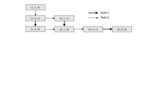
(b) When $n=5$, $n_{0}=3$, $n_{1}=2$, and $k=4$

Figure 1: Hasse diagrams showing: (a) all SERPs of $n=5$ documents in which there are $n_{0}=3$ non-relevant and $n_{1}=2$ relevant documents; and (b) the set of $k=4$ prefixes of those SERPs. The solid arrows indicate the “Rule 1” $\succeq$ relationships, and the dotted arrows show “Rule 2” $\succeq$ relationships. Two relevance grades are assumed, with ${\mbox{\sf{1}}}>{\mbox{\sf{0}}}$.

Figure 1(a) shows the set of $\succeq$ relationships when SERPs of $n=5$ binary document relevance grades with $n_{0}=3$ and $n_{1}=2$ are considered, with “0” and “1” used as shorthand for the document relevance labels G0 and G1 respectively. No Rule 1 relationships are possible when all $n$ documents are included, because the SERPs must be permutations of each other. Figure 1(b) then shows the non-inferiorities that arise when binary SERPs over $n=5$ documents (still with $n_{0}=3$ and $n_{1}=2$) are truncated at $k=4$ for the purposes of evaluation. Now Rule 1 relativities also occur.

All of the relationships shown in Figure 1 are transitive, meaning that SERP pairs that are not linked by a directed path of arrows are incomparable. In both the $n=5$ case and the $k=4$ version the two axiomatic rules are insufficient to impose a preference ordering between $\langle 1,0,0,1,0\rangle$ and $\langle 0,1,1,0,0\rangle$. That is, in the absence of any further information in regard to what it is that users find to be useful, either of these two SERPs might be preferred.

3.3 IR Effectiveness Metrics

Given that context, an effectiveness metric is a categorical to numeric mapping that assigns a real-valued number to each possible class of SERP. Those derived values are often, but not always, in the range $0\ldots 1$. For example, assuming binary document relevance categories with class labels G0 and G1, the simple metric “precision at $k$” (Prec@$k$) is computed as the number of relevant (G1) documents among the first $k$ in the SERP, divided by $k$. Both $\langle 1,0,0,1,0\rangle$ and $\langle 0,1,1,0,0\rangle$ have Prec@$5$ scores of $0.4$, and both have Prec@$4$ scores of $0.5$. But $\langle 0,1,1,0,0\rangle$ is deemed to be better than $\langle 1,0,0,1,0\rangle$ according to Prec@$3$. Moreover, there is a real-world interpretation of Prec@$k$ that can justify its use as a metric: if we suppose that each user of the search system examines exactly the first $k$ documents in each SERP they receive, then Prec@$k$ measures the fraction of documents viewed by the user that are relevant. That is, there is a clear connection between Prec@$k$ and an aspect of the real-world situation that can be argued as being a way of assessing SERP usefulness.

A wide range of other effectiveness metrics have been proposed to augment Prec@$k$, including top-weighted ones that allocate decreasing importance to documents the further they are from the head of the SERP. For example, the metric RR is defined (again, for binary relevance grades) as the reciprocal of the index of the first position in the SERP that contains a G1 document. The same two SERPs $\langle 1,0,0,1,0\rangle$ and $\langle 0,1,1,0,0\rangle$ thus have RR values of $1.0$ and $0.5$ respectively.

With these definitions, an RR value of $0.25$ is possible, but an RR value of $0.75$ is not. Similarly, a Prec@$3$ value of $0.5$ not possible, nor a Prec@$5$ value of $0.35$. Should we be concerned by these absences? Fuhr (2017) and the sequence of papers by Ferrante et al. (2019, 2020, 2021) argue that in the case of RR we most definitely should. In particular, the first of Fuhr’s list of ten “common mistakes” (even if not outright commandments) is “Thou shalt not compute RR”, a directive justified by “…the difference [in score] between ranks $1$ and $2$ is the same as that between ranks $2$ and $\infty$. This means that RR is not an interval scale, it is only an ordinal scale.” We disagree with that conclusion.

3.4 Salaries for SERPs

To set the professorial salary levels listed in Table 2(b) the university in question may have engaged remuneration consultants and asked them to undertake a comparative study of current real-world salary expectations for professors of certain specified abilities. The university knows it has to offer competitive salaries if it is to retain staff, but under the ever-watchful eye of the Provost, doesn’t want to pay too much. That is, we can assume that the correspondences listed in Table 2(b) have been determined to be “market rates” in some way, and drawn from a larger set of initial possibilities that were considered as options. The intervals between the salary points are meaningful; they represent salary differentials that must be paid in a competitive market, measured in dollars.

Suppose that a search engine company – “AmaBaiBinGoo”, perhaps – undertakes a similar market rates study. They run surveys, host focus groups, meet with psychologists, and sponsor IR-related conferences; and conclude from their investigations that the great majority of AmaBaiBinGoo users fall into a “shallow-hasty-youthful” demographic that is highly focused on getting a single correct result for each of their queries. The study participants were also asked to estimate the monetary value of example SERPs, and out of an immense amount of data a set of correspondences between SERP classes (that is, SERP categories constructed using binary document relevance grades G0 and G1, as shown in Figure 1) and perceived values emerges:

SERP type	T1	T2	T3	T4	$\cdots$
Value	$1.00$c	$0.50$c	$0.33$c	$0.25$c	$\cdots$

where the group T1 contains all SERPs that commence with a fully relevant document, $\langle\mbox{\sf{G1}},\ldots\rangle$; group T2 contains all SERPs that have their first relevant document in the second position and commence with $\langle\mbox{\sf{G0}},\mbox{\sf{G1}},\ldots\rangle$; group T3 contains all SERPs that commence with two non-relevant documents and then have a G1-grade document in third position, $\langle\mbox{\sf{G0}},\mbox{\sf{G0}},\mbox{\sf{G1}},\ldots\rangle$; and so on. These grouped SERP categories – T1, T2 and so on – form an ordinal arrangement, because of the positional references to “first” and “second”, but the groups can also still be thought of as categorical labels.

The company’s chief financial officer (CFO) takes great interest in this data. To estimate the possible income should AmaBaiBinGoo move to a user-pays income model, the CFO further assembles a sample of ten recent queries and the SERPs that were returned for them, and constructs this dataset of SERP groups:

$$\{\mbox{\sf{T1}},\mbox{\sf{T3}},\mbox{\sf{T1}},\mbox{\sf{T4}},\mbox{\sf{T3}},\mbox{\sf{T1}},\mbox{\sf{T1}},\mbox{\sf{T1}},\mbox{\sf{T2}},\mbox{\sf{T3}}\}\,\,.$$

The mode of this dataset is T1; in an ordinal sense the median is either T1 or T2; and it is meaningless to ask about the “average SERP category”. But the AmaBaiBinGoo CFO continues, joining the per-SERP revenues estimates from the market research to the sample SERP distribution:

SERP group	T1	T2	T3	T4
Count	$5$	$1$	$3$	$1$
Revenue each	1.00c	0.50c	0.33c	0.25c
Income	5.00c	0.50c	1.00c	0.25c

Summing the bottom row tells them that their current revenue expectation from a user-pays model would be $6.75$c for this sample of ten queries, or $0.675$c per query on average.

Now the critical question arises: is the computation of the average payment per query using this framework a valid computation? We argue that it is, and that it is meaningful in exactly the same way that the average professorial salary is a meaningful value. Both the professorial salaries and the per-SERP payments are on the interval scale of “money”, and by design (and expenditure on consultant fees) reflect their respective real-world situations. Hence, “mean value per SERP” is a valid measurement of search according to its underlying attribute – the usefulness of SERPs to users, provided only that we are willing to equate the attribute of usefulness and the attribute of value. But that equivalence is one of the underpinning assumptions of economics: that the price that someone is willing to pay for goods or a service reflects the utility (that is, usefulness) that they expect to derive from it.

3.5 Different User Behaviors

Table 3: All possible SERPs composed of $n=5$ binary document relevance grades containing $n_{1}=2$ relevant and $n_{0}=3$ non-relevant documents. The metric Prec@$5$ is $0.4$ for all ten SERPs. There are no violations of the $\succeq$ relationships captured by the arrows in Figure 1.

SERP	Evaluated at $n=5$				$k=4$
	RR	RBP0.5	AP	NDCG	Prec@4
$\langle 1,1,0,0,0\rangle$	$1.0000$	$0.7500$	$1.0000$	$1.0000$	$0.5000$
$\langle 1,0,1,0,0\rangle$	$1.0000$	$0.6250$	$0.8333$	$0.9197$	$0.5000$
$\langle 1,0,0,1,0\rangle$	$1.0000$	$0.5625$	$0.7500$	$0.8772$	$0.5000$
$\langle 1,0,0,0,1\rangle$	$1.0000$	$0.5313$	$0.7000$	$0.8503$	$0.2500$
$\langle 0,1,1,0,0\rangle$	$0.5000$	$0.3750$	$0.5833$	$0.6934$	$0.5000$
$\langle 0,1,0,1,0\rangle$	$0.5000$	$0.3125$	$0.5000$	$0.6509$	$0.5000$
$\langle 0,1,0,0,1\rangle$	$0.5000$	$0.2813$	$0.4500$	$0.6241$	$0.2500$
$\langle 0,0,1,1,0\rangle$	$0.3333$	$0.1875$	$0.4167$	$0.5706$	$0.5000$
$\langle 0,0,1,0,1\rangle$	$0.3333$	$0.1563$	$0.3667$	$0.5438$	$0.2500$
$\langle 0,0,0,1,1\rangle$	$0.2500$	$0.0938$	$0.3250$	$0.5013$	$0.2500$

The reader will doubtless have noted that the SERP “pricing” mechanism used in that previous example corresponds to Reciprocal Rank, RR. What if AmaBaiBinGoo’s market research also noted other factors that influence the amount that a user is willing to pay, in addition to the position of the first relevant result in the SERP? For example, suppose that an even more detailed user evaluation (and, who knows, perhaps a deep convoluted neural model as well) reveals that customers are willing to pay $0.50$c if the first document in each SERP is relevant; plus (independently) $0.25$c if the second is relevant; plus another $0.125$c if the third is relevant; and so on; adding up the payments right through the length of the SERP. The “RBP_0.5” column in Table 3 shows the ten different per-SERP values that can arise when this computation is applied to the set of ten $n=5$, $n_{1}=2$ SERPs shown earlier in Figure 1, and places those derived scores beside the corresponding RR values. This new mapping function yields the effectiveness metric rank-biased precision (RBP) with parameter $\phi=0.5$ (Moffat and Zobel, 2008).

Both RR and RBP can be applied to the CFO’s dataset of ten SERPs, with different average scores emerging. Those two averages must not be compared to each other, because they were computed using different mappings and hence different assumptions about value. They may well be correlated, but are not convertible. Nevertheless, both the RR and RBP_0.5 averages over a dataset of categorical SERPs are valid computations in the context of the numeric mappings that were employed when computing them. What the CFO must do is decide which conversion mechanism best captures the value of each SERP class to the members of their user base, that is, which context they believe is the most realistic assessment of value as a surrogate for the underlying attribute of SERP usefulness.

3.6 Users, Models, and Metrics

There are many other possible effectiveness metrics, and more are proposed each year. Table 3 adds two further options to the three that have already been mentioned: average precision, AP (Buckley and Voorhees, 2005; Robertson, 2008); and normalized discounted cumulative gain, NDCG (Järvelin and Kekäläinen, 2002). Each of the five metrics shown is a categorical to numeric mapping, with the numeric targets representing perceived utility, expressed in units of “willing to pay this many cents for a SERP in this category”, and in which “cents” is an imaginary currency that nevertheless has a fixed multiplicative exchange rate that allows conversion to Euros, to USD, to JPY, to RMB, and so on. Just as inches can be converted to parsecs.

The final two – AP and NDCG – are computed somewhat differently to the three already described. They involve a “normalization” step that adjusts the score (payment) associated with each SERP according the maximum amount of relevance available across the collection (in the binary examples used here, expressed by the value $n_{1}$), adding an implication that users are willing to pay increased amounts if relevant documents are relatively scarce, but equally implying that users are somehow aware of the scarcity or not of relevant documents in regard to each query they issue. Note also that all of RBP, AP, and NDCG are top-weighted, meaning that if they are evaluated across the whole collection (that is, on full-length SERPs of length $n$ rather than at-$k$ truncated ones), Rule 2, noted above, results in strict superiority ($\succ$), rather than non-inferiority ($\succeq$).

More generally, most IR metrics have a corresponding user browsing model, which hypothesizes the way in which users interact with each SERP, and the subconscious process they follow as they consume SERPs and assess usefulness – the attribute that we are trying to measure. Thus, one way in which IR effectiveness metrics have been studied is via the development of user browsing models of increasing sophistication (Azzopardi et al., 2018; Zhang et al., 2017; Chapelle et al., 2009; Moffat et al., 2017; Carterette, 2011; Wicaksono and Moffat, 2020). Each such model maps a categorical SERP to a numeric assessment of that SERP’s value on the real number line, usually between $0.0$ and $1.0$ inclusive, in units of “expected utility gained per document inspected”, using the corresponding browsing model as a guide to the manner in which the user consumes, and ends their inspection of, the SERP.

3.7 Equi-Spaced Intervals

As was noted earlier, Fuhr (2017) and Ferrante et al. (2019, 2020, 2021) criticize RR because of this pattern of scores:

first relevant document at rank one, RR${}=1.0$

$\rightarrow$  $-0.5$

first relevant document at rank two, RR${}=0.5$

$\rightarrow$  $-0.5$

no relevant document in top $k$, RR${}=0.0$.

In doing so, they overlook the possibility of users wanting those two intervals to be of equal importance. If users’ perceptions of usefulness concur with the relationship between those three classes of SERP, then RR is an interval scale, with intervals between observed values at different points on the scale that do have the same interpretation in terms of the underlying attribute of usefulness. Any argument that RR is an unsuitable mapping must be justified based on rhetoric (or on data) about user perceptions of usefulness, rather than on non-uniformity of intervals.

Ferrante et al. (2021, page 136193, in connection with their Figure 3) extend that earlier claim, writing: “the real problem with IR evaluation measures is that their scores are not equi-spaced and thus they cannot be interval scales”. This assertion leads them to a proposal that existing metrics be intervalized, by enumerating all possible metric values over truncated SERPs of some defined length ($k=10$, or $k=20$ say, but certainly not $k=100$, because of combinatorial growth issues) and then mapping the ordering implied by those values to a uniform-interval scale to get new versions of those metrics.

To understand the process of intervalization, consider the metric NDCG, already illustrated in Table 3. If we assume that $n_{0},n_{1}\geq 3$ then there are $2^{k}=8$ different binary-grade SERPs possible of length $k=3$, with NDCG$@3$ scores (sorted by score, to three decimal places) of

$$\{0.000,0.235,0.296,0.469,0.531,0.704,0.765,1.000\}\,.$$

That set of eight irregularly-spaced NDCG$@3$ scores would be intervalized to the range $[0,1]$ via the corresponding uniformly-spaced set of eight target values (all multiples of $1/7$, again represented to three decimal places)

$$\{0.000,0.142,0.285,0.428,0.571,0.714,0.857,1.000\}\,.$$

The mapped uniform-interval values would then be used to compute means and as a basis for comparing systems, and to undertake statistical tests, as a derived variant of NDCG$@3$. Similarly, for the metric NDCG$@10$, a set of $1024$ mapped NDCG values would be generated, at uniform intervals of $1/1023$.

We believe that intervalization should regarded with scepticism. There is no requirement in Steven’s typology (Stevens, 1946) that interval scales be restricted to uniform distances between the available measurement points; the requirement is simply that the ratio between pairs of intervals be indicative of the corresponding difference in the underlying attribute. Altering the categorical to numeric mapping used to assign score to SERPs changes the relativities being measured, and thus affects the outcome of any subsequent arithmetic. This effect is especially notable for the metric RR. If truncated rankings of length $k$ are used, mapping to an equi-spaced scale yields:

first relevant at rank one

$\rightarrow$  $-1/k$

first relevant document at rank two

$\rightarrow$  $-1/k$

first relevant at rank three

$\cdots$

first relevant document at rank $k-1$

$\rightarrow$  $-1/k$

first relevant document at rank $k$

$\rightarrow$  $-1/k$

no relevant document in the first $k$

which is logically equivalent to using the rank of the first relevant document as the assessment of SERP usefulness – let’s call it the metric R1, sometimes referred to as “expected search length” (Cooper, 1968). While that is a perfectly valid measure, it probably isn’t a plausible way of measuring the underlying attribute of SERP usefulness. Would a user of an IR system really perceive having the first relevant document at rank $100$ rather than at rank $99$ as being the same amount less useful as is having the first relevant document at rank $2$ rather than at rank $1$? Indeed, R1 is sufficiently obvious as a possible metric that if it were reflective of user perceptions of usefulness, then it would have been in common use in IR evaluation for the last several decades. There has been a reason why R1 has not been used as a measure of SERP quality – because it doesn’t adequately reflect SERP usefulness.

Finally, note that even RBP_0.5 does not guarantee a uniform-interval scale, adding further confusion to the situation. Fuhr (2017) and Ferrante et al. (2019, 2020, 2021) suggest that RBP_0.5 is an example of a valid (by their requirements) interval scale IR metric, because if the runs being evaluated are of length $k$, then all multiples of $2^{-k}$ between $0$ and $1-2^{-k}$ can be generated as metric scores, and hence the measurement points are at uniform intervals. But that conclusion is only correct when $k\leq\min\{n_{0},n_{1}\}$. When complete SERPs to depth $n$ are scored via RBP_0.5, or when truncated SERPs are scored and $n_{1}<k$ (a situation that is by no means improbable), the available set of RBP_0.5 values is not uniform-interval – as is illustrated in Table 3, comparing the sequence $0.565$, $0.531$, and $0.375$, for example. Indeed, when there is a single relevant document for some query (a navigational query (Broder, 2002), with $n_{1}=1$), RBP_0.5 gives this pattern of scores:

relevant at rank one, RBP${}_{0.5}=0.5$

$\rightarrow$  $-0.25$

first relevant document at rank two, RBP${}_{0.5}=0.25$

$\rightarrow$  $-0.25$

no relevant document in the first $k$, RBP${}_{0.5}=0$,

exactly matching (modulo a linear transformation, viz, multiplication by two, a permissible operation) the RR intervals over the same three $k$-truncated SERP classes objected to by Fuhr (2017).

4 Other Considerations

4.1 Related Work

Fuhr’s exposition (Fuhr, 2017) addressing experimental protocols in IR has also been commented on by Sakai (2020) who, amongst other concerns, writes (with acknowledgment to input from Stephen Robertson): “it is also not clear to me whether RR really cannot be considered as an interval-scale measure”, and specifically questions the RR example given by Fuhr (first relevant document at rank one versus first relevant document at rank two versus no relevant document at all) and asks why this cannot ever be congruent with the user’s perception of SERP usefulness, thereby anticipating our own concerns. Sakai (2020) goes on to present agreement rates between human assessors and effectiveness metrics in regard to SERP quality that summarize the results of an experiment by Sakai and Zeng (2019) that compared SERPs in a side by side manner and elicited preferences as to overall usefulness (in this case, via the question “Overall, which SERP is more relevant to the query?”). It is experiments such as these that will establish which effectiveness metrics best correlate with user perceptions of SERP usefulness for various search applications and different sub-demographics of users (Sakai and Zeng, 2021). Similarly, consideration of perceived user experience is what has driven much of the recent development of effectiveness metrics – see Moffat et al. (2017), Zhang et al. (2017), and Azzopardi et al. (2018), for example.

There has also been followup commentary in regard to Stevens’ original paper (Stevens, 1946) about scales of measurement. The contribution by Lord (1953) has already been noted; amongst many others the evaluations by Townsend and Ashby (1984) and Velleman and Wilkinson (1993) also help delineate some of the issues that have emerged when considering scales of measurement and their implications. Scholten and Borsboom (2009) provide a careful assessment of the role of Lord’s claimed “counter example” in regard to Stevens’ taxonomy of measurement scales.

In addition to the studies already discussed in Section 3, a range of work has considered the underpinning measurements involved in IR. For example, Busin and Mizzaro (2013) consider measurement scales and SERP orderings, developing and extending axiomatic relationships akin to the “Rule 1” and “Rule 2” given above; and Ferrante et al. (2015) undertake a similar exploration. In a related study, Moffat (2013) considers effectiveness metrics in terms of a suite of seven numeric properties that they might possess. Other work – for example, Turpin and Hersh (2001), Turpin and Scholer (2006), Sanderson et al. (2010), Bailey et al. (2010), Liu et al. (2018), and Zhang et al. (2020) – has considered the extent to which whole-of-SERP usefulness is adequately captured by current effectiveness metrics.

4.2 Use of Recall Base

Fuhr (2017) and Ferrante et al. (2019, 2020, 2021) note the difficulties created by the use in some metrics of what they term the “recall base”, the number RB of relevant (assuming only binary relevance grades) documents in the collection for the topic in question, denoted in Section 3 as the quantity $n_{1}$. From the point of view of Fuhr and Ferrante et al., those difficulties arise because normalization by RB means that the set of generable measurement points for any query in a set of topics might not numerically align with the available measurement points for other topics that have different values for RB. But it is worth noting that the recall base affects the available measurements even when RB is not a visible component of the effectiveness metric. To observe this, consider Table 3 again. It lists the ten possible SERP classes for a collection of $n=5$ documents and for queries with $n_{1}=2$ relevant documents in the collection, together with metric score according to five metrics. If another topic for the same test collection has $n_{1}=1$, the RBP_0.5 scores are limited to the set $\{0.500,0.250,0.125,0.063,0.031\}$, none of which align with the set of available $n_{1}=2$ RBP_0.5 scores listed in Table 3.

Moreover, even when truncated rankings are considered, with (say) $k=2$ used to calculate the scores, a topic for which $n_{1}=1$ is unable to deliver a RBP_0.5 score of $0.75$. If RBP_0.5 is to be used across a collection of topics, and if exactly the same set of measurement points must be available for every topic, then the SERP truncation length $k$ must satisfy $k\leq\min_{i}n_{1,i}$, where $n_{1,i}$ is the $n_{1}$ recall base associated with the $i$ th topic. This places a severe limitation on any experiments making use of that collection. (The same restriction also applies to $n_{0}$, but in most retrieval environments $n_{1}$ is smaller than $n_{0}$ by several orders of magnitude.)

Our contention in this work is that the measurement scale is always the positive real number line, and hence that no question of alignment (or not) of measurement points across sets of topics arises. On the other hand, there are other reasons to eschew metrics that make use of the recall base, based on the desire for effectiveness metrics to reflect plausible user behaviors, and the user’s inability to actually know the value $n_{1}$ as they consider the SERP (Moffat and Zobel, 2008; Zobel et al., 2009; Lu et al., 2016).

4.3 Graded Relevance and Gain Mappings

The discussion above focused on binary-level document relevance labels, but the same points apply to multi-level labels of the kind suggested in Table 2(d). Multi-level evaluations normally make use of two mapping stages. The first converts ordinal document relevance classes to numeric gains via a gain mapping function $N(\cdot)$ that converts ordinal document relevance grades to gain values in $0\ldots 1$, as shown, for example, in Table 2(d). The second mapping then takes an $n$- or $k$-vector of numeric gain values, combines them in a way that discounts gains as ranks increase, and generates a single numeric score. The metrics discounted cumulative gain (DCG) and normalized discounted cumulative gain (NDCG) (Järvelin and Kekäläinen, 2002) make quite deliberate use of real-valued document gains, as do RBP (Moffat and Zobel, 2008) and expected reciprocal rank (ERR) (Chapelle et al., 2009), with the goal of providing more nuanced effectiveness measurements, and hence the ability to respond with more sensitivity to perceived differences in SERP usefulness (Sormunen, 2002). Average precision can also be broadened to make use of graded document relevance categories (Robertson et al., 2010; Dupret and Piwowarski, 2010).

The complex inter-relationships between the range of gain mappings that might be employed, and then the metric mapping itself, further mean that metric scores will not (and as is our firm contention here, need not) result in uniform-interval measurements.

Gain mappings are also measurements, of course, pertaining to the usefulness of individual documents. For example, the ordinal class labels listed in Table 2(d) might be included in a handbook provided to assessors as part of their training, along with detailed descriptions and examples. Document gain labels – the $r_{i}$ values used to compute effectiveness metrics – can also be more directly measured. For example, magnitude estimation techniques (Turpin et al., 2015; Maddalena et al., 2017), side-by-side preference elicitation (Carterette et al., 2008; Sanderson et al., 2010; Yang et al., 2018; Arabzadeh et al., 2021), and ordinal scales in which the class labels are numbers (Roitero et al., 2018) can all be used to develop numeric document gain labels.

4.4 Statistical Tests

An important component of IR evaluation is the use of statistical tests (see, for example, Smucker et al. (2007), Sakai (2016), and Urbano et al. (2019)). The appropriateness of any particular test depends in part on the distributional conditions required by that test, and it should be noted that our argument here in regard to metric values being numbers that can be averaged is most definitely not an argument that all metrics can be tested with any particular statistical test. Thoughtful selection of a statistical test, and, if necessary, verification of any required distributional conditions governing its applicability, must always be a critical part of IR experimental design. On the other hand, choosing an effectiveness metric because it is amenable to a particular statistical test represents “the tail wagging the dog” (pun intended), and is not a course of action that should be considered. The metric must be chosen first, and only then can the statistical test be selected.

Similarly, we have no concerns with Fuhr’s seventh rule, covering the need for multiple hypothesis adjustments, but note that in the case of test collection reuse it cannot always be properly achieved. Craswell et al. (2021) provide an overview of some of these issues, and Sakai (2020) has also voiced opinions in support of Fuhr’s comments in regard to statistical testing.

5 Conclusions

We have discussed the role of interval scale measures in information retrieval evaluation and, via a sequence of examples, presented our view that all IR effectiveness metrics can be considered to be interval scale measurements, provided only that the mapping from SERP categories to numeric scores has a real-world basis and can be argued in some way as corresponding to the underlying usefulness of each SERP, as experienced by the users of that IR system. That is, while care needs to be exercised when choosing the metric that best fits the user experience for any particular IR application (for example, the “shallow-hasty-youthful” users that form the AmaBaiBinGoo demographic), once that match has been decided, the values calculated by the effectiveness metric may be used as “simple numbers”, without regard to their origins in a categorical-scale SERP dataset.

Metric choice is a critically important design decision in any IR experiment, and different metrics might lead to different outcomes from a planned experiment. But the choice between metrics should determined by the projected user behavior and their implicit evaluation of “usefulness” relative to their search task, and not because of the regularity or otherwise of the gaps between adjacent numeric values generated over the universe of categorical SERP classes, and nor as a consequence of amenability or system separability associated with any particular statistical test.

In addition, we have argued that the proposed “intervalization” of current IR effectiveness metrics is neither required nor helpful. If the raw metric value is indeed a defensible measurement of SERP usefulness and corresponds to the user experience when they are presented with a member of that SERP category, then equi-intervalizing those measurements via a different categorical to numeric mapping must of necessity distort and alter any findings that arise, and thus risks masking what would otherwise be valid conclusions. And if the raw metric is not a defensible measurement of SERP usefulness, then equi-intervalizing its scores seems unlikely to improve the situation.

Acknowledgment

Joel Mackenzie, Tetsuya Sakai, Falk Scholer, and Justin Zobel provided useful input. This work was supported under the Australian Research Council’s Discovery Projects funding scheme (project DP190101113). Science proceeds via debate, and we are grateful to be part of a community in which debate is not only possible, but actively welcomed.

Disclosure

The author has no other relevant financial or non-financial interests to disclose.

References

- Arabzadeh et al. [2021] N. Arabzadeh, A. Vtyurina, X. Yan, and C. L. A. Clarke. Shallow pooling for sparse labels. arXiv:2109.00062, Aug. 2021.
- Azzopardi et al. [2018] L. Azzopardi, P. Thomas, and N. Craswell. Measuring the utility of search engine result pages: An information foraging based measure. In Proc. ACM Int. Conf. on Research and Development in Information Retrieval (SIGIR), pages 605–614, 2018.
- Bailey et al. [2010] P. Bailey, N. Craswell, R. W. White, L. Chen, A. Satyanarayana, and S. M. M. Tahaghoghi. Evaluating whole-page relevance. In Proc. ACM Int. Conf. on Research and Development in Information Retrieval (SIGIR), pages 767–768, 2010.
- Broder [2002] A. Z. Broder. A taxonomy of web search. SIGIR Forum, 36(2):3–10, 2002.
- Buckley and Voorhees [2005] C. Buckley and E. M. Voorhees. Retrieval system evaluation. In E. M. Voorhees and D. K. Harman, editors, TREC: Experiment and Evaluation in Information Retrieval, chapter 3. The MIT Press, 2005.
- Busin and Mizzaro [2013] L. Busin and S. Mizzaro. Axiometrics: An axiomatic approach to information retrieval effectiveness metrics. In Proc. Int. Conf. on Theory of Information Retrieval (ICTIR), pages 1–8, 2013.
- Carterette [2011] B. Carterette. System effectiveness, user models, and user utility: A conceptual framework for investigation. In Proc. ACM Int. Conf. on Research and Development in Information Retrieval (SIGIR), pages 903–912, 2011.
- Carterette et al. [2008] B. Carterette, P. N. Bennett, D. M. Chickering, and S. T. Dumais. Here or there: Preference judgments for relevance. In Proc. European Conf. on Information Retrieval (ECIR), pages 16–27, 2008.
- Chapelle et al. [2009] O. Chapelle, D. Metzler, Y. Zhang, and P. Grinspan. Expected reciprocal rank for graded relevance. In Proc. ACM Int. Conf. on Information and Knowledge Management (CIKM), pages 621–630, 2009.
- Cooper [1968] W. S. Cooper. Expected search length: A single measure of retrieval effectiveness based on the weak ordering action of retrieval systems. American Documentation, 19(1):30–41, 1968.
- Craswell et al. [2021] N. Craswell, B. Mitra, E. Yilmaz, D. Campos, and J. Lin. MS MARCO: Benchmarking ranking models in the large-data regime. In Proc. ACM Int. Conf. on Research and Development in Information Retrieval (SIGIR), pages 1566–1576, 2021.
- Dupret and Piwowarski [2010] G. Dupret and B. Piwowarski. A user behavior model for average precision and its generalization to graded judgments. In Proc. ACM Int. Conf. on Research and Development in Information Retrieval (SIGIR), pages 531–538, 2010.
- Ferrante et al. [2015] M. Ferrante, N. Ferro, and M. Maistro. Towards a formal framework for utility-oriented measurements of retrieval effectiveness. In Proc. Int. Conf. on Theory of Information Retrieval (ICTIR), pages 21–30, 2015.
- Ferrante et al. [2019] M. Ferrante, N. Ferro, and S. Pontarollo. A general theory of IR evaluation measures. IEEE Transactions on Knowledge and Data Engineering, 31(3):409–422, 2019.
- Ferrante et al. [2020] M. Ferrante, N. Ferro, and E. Losiouk. How do interval scales help us with better understanding IR evaluation measures? Information Retrieval, 23(3):289–317, 2020.
- Ferrante et al. [2021] M. Ferrante, N. Ferro, and N. Fuhr. Towards meaningful statements in IR evaluation: Mapping evaluation measures to interval scales. IEEE Access, 9:136182–136216, 2021.
- Fuhr [2017] N. Fuhr. Some common mistakes in IR evaluation, and how they can be avoided. SIGIR Forum, 51(3):32–41, 2017.
- Hays [1994] W. Hays. Statistics. Harcourt Brace, New York, fifth edition, 1994.
- Järvelin and Kekäläinen [2002] K. Järvelin and J. Kekäläinen. Cumulated gain-based evaluation of IR techniques. ACM Trans. on Information Systems, 20(4):422–446, 2002.
- Liu et al. [2018] M. Liu, Y. Liu, J. Mao, C. Luo, M. Zhang, and S. Ma. “Satisfaction with failure” or “unsatisfied success”: Investigating the relationship between search success and user satisfaction. In Proc. Conf. on the World Wide Web (WWW), pages 1533–1542, 2018.
- Lord [1953] F. M. Lord. On the statistical treatment of football numbers. Amer. Psychol., 8(12):750–751, 1953.
- Lu et al. [2016] X. Lu, A. Moffat, and J. S. Culpepper. The effect of pooling and evaluation depth on IR metrics. Information Retrieval, 19(4):416–445, 2016.
- Maddalena et al. [2017] E. Maddalena, S. Mizzaro, F. Scholer, and A. Turpin. On crowdsourcing relevance magnitudes for information retrieval evaluation. ACM Trans. on Information Systems, 35(3):19:1–19:32, 2017.
- Moffat [2013] A. Moffat. Seven numeric properties of effectiveness metrics. In Proc. Asia Information Retrieval Societies Conf. (AIRS), pages 1–12, 2013.
- Moffat and Zobel [2008] A. Moffat and J. Zobel. Rank-biased precision for measurement of retrieval effectiveness. ACM Trans. on Information Systems, 27(1):2.1–2.27, 2008.
- Moffat et al. [2017] A. Moffat, P. Bailey, F. Scholer, and P. Thomas. Incorporating user expectations and behavior into the measurement of search effectiveness. ACM Trans. on Information Systems, 35(3):24:1–24:38, 2017.
- Robertson [2008] S. E. Robertson. A new interpretation of average precision. In Proc. ACM Int. Conf. on Research and Development in Information Retrieval (SIGIR), pages 689–690, 2008.
- Robertson et al. [2010] S. E. Robertson, E. Kanoulas, and E. Yilmaz. Extending average precision to graded relevance judgments. In Proc. ACM Int. Conf. on Research and Development in Information Retrieval (SIGIR), pages 603–610, 2010.
- Roitero et al. [2018] K. Roitero, E. Maddalena, G. Demartini, and S. Mizzaro. On fine-grained relevance scales. In Proc. ACM Int. Conf. on Research and Development in Information Retrieval (SIGIR), pages 675–684, 2018.
- Sakai [2016] T. Sakai. Statistical significance, power, and sample sizes: A systematic review of SIGIR and TOIS, 2006–2015. In Proc. ACM Int. Conf. on Research and Development in Information Retrieval (SIGIR), pages 5–14, 2016.
- Sakai [2020] T. Sakai. On Fuhr’s guideline for IR evaluation. SIGIR Forum, 54(1):12:1–12:8, 2020.
- Sakai and Zeng [2019] T. Sakai and Z. Zeng. Which diversity evaluation measures are “good”? In Proc. ACM Int. Conf. on Research and Development in Information Retrieval (SIGIR), pages 595–604, 2019.
- Sakai and Zeng [2021] T. Sakai and Z. Zeng. Retrieval evaluation measures that agree with users’ SERP preferences: Traditional, preference-based, and diversity measures. ACM Trans. on Information Systems, 39(2):14:1–14:35, 2021.
- Sanderson [2010] M. Sanderson. Test collection based evaluation of information retrieval systems. Foundations & Trends in Information Retrieval, 4(4):247–375, 2010.
- Sanderson et al. [2010] M. Sanderson, M. L. Paramita, P. D. Clough, and E. Kanoulas. Do user preferences and evaluation measures line up? In Proc. ACM Int. Conf. on Research and Development in Information Retrieval (SIGIR), pages 555–562, 2010.
- Scholten and Borsboom [2009] A. Z. Scholten and D. Borsboom. A reanalysis of Lord’s statistical treatment of football numbers. J. Math. Psych., 53(2):69–75, 2009.
- Smucker et al. [2007] M. D. Smucker, J. Allan, and B. Carterette. A comparison of statistical significance tests for information retrieval evaluation. In Proc. ACM Int. Conf. on Information and Knowledge Management (CIKM), pages 623–632, 2007.
- Sormunen [2002] E. Sormunen. Liberal relevance criteria of TREC: Counting on negligible documents? In Proc. ACM Int. Conf. on Research and Development in Information Retrieval (SIGIR), pages 324–330, 2002.
- Stevens [1946] S. S. Stevens. On the theory of scales of measurement. Science, 103(2684):677–680, 1946.
- Townsend and Ashby [1984] J. T. Townsend and F. G. Ashby. Measurement scales and statistics: The misconception misconceived. Psych. Bull., pages 394–401, 1984.
- Turpin and Hersh [2001] A. Turpin and W. R. Hersh. Why batch and user evaluations do not give the same results. In Proc. ACM Int. Conf. on Research and Development in Information Retrieval (SIGIR), pages 225–231, 2001.
- Turpin and Scholer [2006] A. Turpin and F. Scholer. User performance versus precision measures for simple search tasks. In Proc. ACM Int. Conf. on Research and Development in Information Retrieval (SIGIR), pages 11–18, 2006.
- Turpin et al. [2015] A. Turpin, F. Scholer, S. Mizzaro, and E. Maddalena. The benefits of magnitude estimation relevance assessments for information retrieval evaluation. In Proc. ACM Int. Conf. on Research and Development in Information Retrieval (SIGIR), pages 565–574, 2015.
- Urbano et al. [2019] J. Urbano, H. Lima, and A. Hanjalic. Statistical significance testing in information retrieval: An empirical analysis of type I, type II and type III errors. In Proc. ACM Int. Conf. on Research and Development in Information Retrieval (SIGIR), pages 505–514, 2019.
- Velleman and Wilkinson [1993] P. F. Velleman and L. Wilkinson. Nominal, ordinal, interval, and ratio typologies are misleading. The American Statistician, 47(1):65–72, 1993.
- Wicaksono and Moffat [2020] A. F. Wicaksono and A. Moffat. Metrics, user models, and satisfaction. In Proc. Conf. on Web Search and Data Mining (WSDM), pages 654–662, 2020.
- Yang et al. [2018] Z. Yang, A. Moffat, and A. Turpin. Pairwise crowd judgments: Preference, absolute, and ratio. In Proc. Australasian Document Computing Symp. (ADCS), pages 3.1–3.8, 2018.
- Zhang et al. [2017] F. Zhang, Y. Liu, X. Li, M. Zhang, Y. Xu, and S. Ma. Evaluating web search with a bejeweled player model. In Proc. ACM Int. Conf. on Research and Development in Information Retrieval (SIGIR), pages 425–434, 2017.
- Zhang et al. [2020] F. Zhang, J. Mao, Y. Liu, X. Xie, W. Ma, M. Zhang, and S. Ma. Models versus satisfaction: Towards a better understanding of evaluation metrics. In Proc. ACM Int. Conf. on Research and Development in Information Retrieval (SIGIR), page 379–388, 2020.
- Zobel et al. [2009] J. Zobel, A. Moffat, and L. A. F. Park. Against recall: Is it persistence, cardinality, density, coverage, or totality? SIGIR Forum, 43(1):3–15, 2009.