A conditional gradient homotopy method with applications to Semidefinite Programming

Abstract

We propose a new homotopy-based conditional gradient method for solving convex optimization problems with a large number of simple conic constraints. Instances of this template naturally appear in semidefinite programming problems arising as convex relaxations of combinatorial optimization problems. Our method is a double-loop algorithm in which the conic constraint is treated via a self-concordant barrier, and the inner loop employs a conditional gradient algorithm to approximate the analytic central path, while the outer loop updates the accuracy imposed on the temporal solution and the homotopy parameter. Our theoretical iteration complexity is competitive when confronted to state-of-the-art SDP solvers, with the decisive advantage of cheap projection-free subroutines. Preliminary numerical experiments are provided for illustrating the practical performance of the method.

1 Introduction

In this paper we investigate a new algorithm for solving a large class of convex optimization problems with conic constraints of the following form:

$$\min_{x}g(x)\quad\text{s.t. }x\in\mathsf{X},\mathcal{P}(x)\in\mathsf{K}\subseteq\mathsf{H}.$$ (P)

The objective function $g:\mathsf{E}\to(-\infty,\infty]$ is assumed to be closed, convex, and lower semi-continuous, $\mathsf{X}\subseteq\mathsf{E}$ is a compact convex set, and $\mathcal{P}:\mathsf{E}\to\mathsf{H}$ is an affine mapping between two finite-dimensional Euclidean vector spaces $\mathsf{E}$ and $\mathsf{H}$, and $\mathsf{K}$ is a closed convex pointed cone. Problem (P) is sufficiently generic to cover many optimization settings considered in the literature.

Example 1.1 (Packing SDP).

The model template (P) covers the large class of packing semidefinite programs (SDPs) [22, 12]. In this problem class we have $\mathsf{E}=\mathbb{S}^{n}$ – the space of symmetric $n\times n$ matrices, a collection of positive semidefinite input matrices ${\mathbf{A}}_{1},\ldots,{\mathbf{A}}_{m}\in\mathbb{S}^{n}_{+}$, with constraints given by $\mathcal{P}(\mathbf{X})=[1-\operatorname{tr}({\mathbf{A}}_{1}\mathbf{X});\ldots;1-\operatorname{tr}({\mathbf{A}}_{m}\mathbf{X})]^{\top}$ and $\mathsf{K}=\mathbb{R}^{m}_{+}$, coupled with the objective function $g(\mathbf{X})=\operatorname{tr}(C\mathbf{X})$ and the set $\mathsf{X}=\{\mathbf{X}\in\mathbb{S}^{n}_{+}|\operatorname{tr}(\mathbf{X})\leq\rho\}$. Special instances of packing SDPs include the MaxCut SDP relaxation of [17], the Lovasz-$\theta$ function SDP, among many others; see [21].

Example 1.2 (Covering SDP).

A dual formulation of the packing SDP is the covering problem [12]. In its normalized version, the problem reads as

$$\min_{x}\sum_{i=1}^{m}x_{i}\quad\text{s.t.:}\sum_{i=1}^{m}x_{i}{\mathbf{A}}_{i}-\mathbf{I}\succeq 0,x\in\mathbb{R}^{m}_{+},$$

where ${\mathbf{A}}_{1},\ldots,{\mathbf{A}}_{m}\in\mathbb{S}^{n}_{+}$ are given input matrices. This can be seen as a special case of problem (P) with $g(x)=\sum_{i=1}^{m}x_{i},\mathcal{P}(x)=\sum_{i=1}^{m}x_{i}{\mathbf{A}}_{i}-\mathbf{I},\mathsf{K}=\mathbb{S}^{n}_{+},\mathsf{H}=\mathbb{S}^{n},\mathsf{E}=\mathbb{R}^{m}$, and the constraint set $\mathsf{X}=\{x\in\mathbb{R}^{m}_{+}|\sum_{i=1}^{m}x_{i}\leq\rho\}$ for some large $\rho$ added to the problem for the compactification purposes.

Example 1.3 (Relative Cone Programming).

Relative entropy programs are conic optimization problems in which a linear functional of a decision variable is minimized subject to linear constraints and conic constraints specified by a relative entropy cone. The relative entropy cone is defined for triples $(u,v,w)\in\mathbb{R}^{n}\times\mathbb{R}^{n}\times\mathbb{R}^{n}$ via Cartesian products of the following elementary cone

$$\mathsf{K}^{(1)}_{\text{RE}}=\{(\nu,\lambda,\delta)\in\mathbb{R}_{+}\times\mathbb{R}_{+}\times\mathbb{R}|-\nu\log\left(\frac{\lambda}{\nu}\right)\leq\delta\}.$$

As the function $\mathbb{R}^{2}_{++}\ni(\nu,\lambda)\mapsto-\nu\log(\lambda/\nu)$ is the perspective transform of the negative logarithm, we know that it is a convex function [3]. Hence, $\mathsf{K}^{(1)}_{\text{RE}}$ is a convex cone. The relative entropy cone is accordingly defined as $\mathsf{K}=\prod_{i=1}^{n}\mathsf{K}^{(1)}_{\text{RE}}$.

Example 1.4 (Relative Entropy entanglement).

The relative entropy of entanglement (REE) is an important measure for entanglement for a given quantum state in quantum information theory [29]. A major problem in quantum information theory is obtain accurate bounds on the REE. In [42] the following problem is used to obtain a lower bound to the REE:

$$\min_{x}g(x)=\operatorname{tr}[\rho(\log(\rho)-\log(x))]$$

s.t.: $$x\in\mathbb{H}^{n}_{+},\operatorname{tr}(x)=1,\;\mathcal{P}(x)\in\mathbb{H}^{n}_{+},$$

where $\mathbb{H}^{n}_{+}$ is the cone of $n\times n$ Hermitian positive semi-definite matrices, and $\mathcal{P}(x)$ is the so-called partial transpose operator, which is a linear symmetric operator (see [20]). $\rho\in\mathbb{H}^{n}_{+}$ is a given quantum reference state. We obtain a problem of the form (P), upon the identification $\mathsf{E}=\mathbb{H}^{n}$ the space of $n\times n$ Hermitian matrices, and $\mathsf{K}=\mathbb{H}^{n}_{+}$, and $\mathsf{X}=\{x\in\mathsf{E}|x\in\mathbb{H}^{n}_{+},\operatorname{tr}(x)=1\}$.

The model template (P) can be solved with moderate accuracy using fast proximal gradient methods, like FISTA and related acceleration tricks [10]. In this formalism, the constraints imposed on the optimization problem have to be included in proximal operators which essentially means that one can calculate a projection onto the feasible set. Unfortunately, the computation of proximal operators can impose a significant burden and even lead to intractability of gradient-based methods. This is in particular the case in SDPs with a large number of constraints and decision variables, such as in convex relaxations of NP-hard combinatorial optimization problems [26]. Other prominent examples in machine learning are $k$-means clustering [30], $k$-nearest neighbor classification [33], sparse PCA [6], kernel learning [25], among many others. In many of these mentioned applications, it is not only the size of the problem that challenges the application of off-the-shelve solvers, but also the desire to obtain sparse solutions. As a result, the Conditional Gradient (CndG) method [15] has seen renewed interest in large-scale convex programming, since it requires only a Linear minimization oracle (LMO) in each iteration. Compared to proximal methods, CndG features significantly reduced computational costs (e.g. when $\mathsf{X}$ is a spectrahedron), tractability and interpretability (e.g. it generates solutions as a combination of atoms of $\mathsf{X})$.

Our approach

In this paper we propose a CndG framework for solving (P) with rigorous iteration complexity guarantees. Our approach retains the simplicity of CndG, but allows to disentangle the different sources of complexity describing the problem. Specifically, we study the performance of a new homotopy/path-following method, which iteratively approaches a solution of problem (P). To develop the path-following argument we start by decomposing the feasible set into two components. We assume that $\mathsf{X}$ is a compact convex set which admits efficient applications of CndG. The challenging constraints are embodied by the membership condition $\mathcal{P}(x)\in\mathsf{K}$. These are conic restrictions on the solution, and in typical applications of our method we have to manage a lot of them. Our approach deals with these constraints via a logarithmically homogeneous barrier for the cone $\mathsf{K}$. [28] introduced this class of functions in connection with polynomial-time interior point methods. It is a well-known fact that any closed convex cone admits a logarithmically homogeneous barrier (the universal barrier) [28, Thm. 2.5.1]. A central assumption of our approach is that we have a practical representation of a logarithmically homogenous barrier for the cone $\mathsf{K}$. As many restrictions appearing in applications are linear or PSD inequalities, this assumption is rather mild. Exploiting the announced decomposition, we approximate the target problem (P) by a family of parametric penalty-based composite convex optimization problems formulated in terms of the potential function

$$\min_{x\in\mathsf{X}}\{V_{t}(x):=\frac{1}{t}F(x)+g(x)\}.$$ (1.1)

This potential function involves a path-following/homotopy parameter $t>0$, and $F$ is a barrier function defined over the set $\mathcal{P}^{-1}(\mathsf{K})$. By minimizing the function $V_{t}$ over the set $\mathsf{X}$ for a sequence of increasing values of $t$, we can trace the analytic central path $z^{\ast}(t)$ of (1.1) as it converges to a solution of (P). The practical implementation of this path-following scheme is achieved via a two-loop algorithm in which the inner loop performs a number of CndG updating steps on the potential function $V_{t}$, and the outer-loop readjusts the parameter $t$ a well as the desired tolerance imposed on the CndG-solver. Importantly, unlike existing primal-dual methods for (P) (e.g. [39]), our approach generates a sequence of feasible points for the original problem (P).

Comparison to the literature

Exact homotopy/path-following methods were developed in statistics and signal processing in the context of the $\ell_{1}$-regularized least squares problem (LASSO) [32] to compute the entire regularization path. Relatedly, approximate homotopy methods have been studied in this context as well [19, 34], and superior empirical performance has been reported for seeking sparse solutions. [35] is the first reference which investigates the complexity of a proximal gradient homotopy method for the LASSO problem. To our best knowledge, our paper provides the first complexity analysis of a homotopy CndG algorithm to compute an approximate solution close to the analytic central path for the optimization template (P). Our analysis is heavily influenced by recent papers [41] and [40]. They study a generalized CndG algorithm designed for solving a composite convex optimization problem, in which the smooth part is given by a logarithmically homogeneous barrier. Unlike [41], we analyze a more complicated dynamic problem in which the objective changes as we update the penalty parameter, and we propose important practical extensions including line-search and inexact-LMO versions of the CndG algorithm for reducing the potential function (1.1). Furthermore, we analyze the complexity of the whole path-following process in order to approximate a solution to the initial non-penalized problem (P).

Main Results

One of the challenging questions is how to design a penalty parameter updating schedule, and we develop a practical answer to this question. Specifically, our contributions can be summarized as follows:

• We introduce a simple CndG framework for solving problem (P) and prove that it achieves a $\tilde{O}(\varepsilon^{-2})$ iteration complexity, where $\tilde{O}(\cdot)$ hides polylogarithmic factors (Theorem 3.4).

• We provide two extensions for the inner-loop CndG algorithm solving the potential minimization problem (1.1): a line-search and an inexact-LMO version. For both, we show that the complexity of the inner and the outer loop are the same as in the basic variant up to constant factors.

• We present key instances of our framework, including instances of SDPs arising from convex relaxations of NP-hard combinatorial optimization problems, and provide promising results of the numerical experiments.

Direct application of existing CndG frameworks [38, 39] for solving (P) would require projection onto $\mathsf{K}$, which may be complicated if, e.g., $\mathsf{K}$ is a PSD cone. Moreover, these algorithms do not produce feasible iterates but rather approximate solutions with primal optimality and dual feasibility guarantees. For specific instances of SDPs, the theoretical complexity achieved by our method matches or even improves the state-of-the-art iteration complexity results reported in the literature. For packing and covering types of SDPs, the state-of-the-art upper complexity bound reported in [12] is worse than ours since their algorithm has complexity $\tilde{O}(C_{1}\varepsilon^{-2.5}+C_{2}\varepsilon^{-2})$, where $C_{1},C_{2}$ are constants depending on the problem data. For SDPs with linear equality constraints and spectrahedron constraints, the primal-dual method CGAL [39] produces approximately optimal and approximately feasible points in $O(\varepsilon^{-2})$ iterations with high probability. Our method is purely primal, generating feasible points anytime, and deterministic. At the same time, our method shares the same iteration complexity as CGAL and can deal with additional conic constraints embodied by the membership restriction $\mathcal{P}(x)\in\mathsf{K}$. We expect that this added feature will allow us to apply our method to handle challenging scientific computing questions connected to the quantum information theory, such as bounding the relative entropy of entanglement of quantum states (cf. Example 1.4 and [42, 13, 14]). Applications to this important setting are the subject of current investigations.

Organization of the paper

This paper is organized as follows: Section LABEL:sec:notation fixes the notation and terminology we use throughout this paper. Section LABEL:sec:alg presents the basic algorithm under consideration in this paper. In section 3.5 we describe an inexact version of our basic homotopy method. Section 5 reports the performance of our method in solving relevant examples of SDPs and gives some first comparisons with existing approaches. In particular, numerical results on the MaxCut and the mixing time problem of a finite Markov Chain are reported there. Section 4 contains a detailed complexity analysis of our scheme when an exact LMO is available. The corresponding statements under our inexact LMO is performed in Appendix A. The supplementary materials B contains further results on the numerical experiments.

2 Notation & Preliminaries

Let $\mathsf{E}$ be a finite-dimensional Euclidean vector space, $\mathsf{E}^{\ast}$ its dual space, which is formed by all linear functions on $\mathsf{E}$. The value of function $s\in\mathsf{E}^{\ast}$ at $x\in\mathsf{E}$ is denoted by $\langle s,x\rangle$. Let $B:\mathsf{E}\to\mathsf{E}^{\ast}$ be a positive definite self-adjoint operator. Define the norms

$$\lVert h\rVert_{B}=\langle Bh,h\rangle^{1/2}\qquad h\in\mathsf{E},$$

$$\lVert s\rVert_{B}^{\ast}=\langle s,B^{-1}s\rangle^{1/2}\qquad s\in\mathsf{E}^{\ast},$$

$$\lVert A\rVert=\max_{\lVert h\rVert\leq 1}\lVert Ah\rVert_{\ast}\qquad A:\mathsf{E}\to\mathsf{E}^{\ast}.$$

For a smooth function $f:\operatorname{dom}(f)\to\mathbb{R}$ with convex and open domain $\operatorname{dom}(f)\subseteq\mathsf{E}$, we denote by $\nabla f(x)$ its gradient, by $\nabla^{2}f(x)$ its Hessian evaluated at $x\in\mathsf{E}$. Note that

$$\nabla f(x)\in\mathsf{E}^{\ast},\quad\nabla^{2}f(x)h\in\mathsf{E}^{\ast}\quad x\in\operatorname{dom}(f),h\in\mathsf{E}.$$

In what follows, we often work with directional derivatives. For $p\geq 1$, denote by

$$f^{p}(x)[h_{1},\ldots,h_{p}]$$

the directional derivative of function $f$ at $x$ along directions $h_{i}\in\mathsf{E},i=1,\ldots,p.$ In particular, we denote by

$$f^{\prime}(x)[h]=f^{1}(x)[h],\;f^{\prime\prime}(x)[h_{1},h_{2}]=f^{2}(x)[h_{1},h_{2}],\;f^{\prime\prime\prime}(x)[h_{1},h_{2},h_{3}]=f^{3}(x)[h_{1},h_{2},h_{3}]$$

for $x\in\operatorname{dom}(f),h_{i}\in\mathsf{E},i=1,2,3.$

2.1 Self-Concordant Functions

Let $\mathsf{Q}$ be an open and convex subset of $\mathsf{E}$. A function $f:\mathsf{E}\to(-\infty,\infty]$ is self-concordant (SC) on $\mathsf{Q}$ if $f\in{\mathbf{C}}^{3}(\mathsf{Q})$ and for all $x\in\mathsf{Q},h\in\mathsf{E}$, we have $\lvert f^{\prime\prime\prime}(x)[h,h,h]\rvert\leq 2(f^{\prime\prime}(x)[h,h])^{3/2}.$ In case where $\operatorname{cl}(\mathsf{Q})$ is a closed convex cone, more structure is available to us. We call $f$ a $\nu$-canonical barrier for $\mathsf{Q}$, denoted by $f\in\mathcal{B}_{\nu}(\mathsf{Q})$, if it is SC and

$$\forall(x,t)\in\mathsf{Q}\times(0,\infty):\quad f(tx)=f(x)-\nu\log(t).$$

From [28, Prop. 2.3.4], the following properties are satisfied by a $\nu$-canonical barrier for each $x\in\mathsf{Q},h\in\mathsf{E},t>0$:

$$f^{\prime}(tx)=t^{-1}f^{\prime}(x),$$ (2.1)

$$f^{\prime}(x)[h]=-f^{\prime\prime}(x)[x,h],$$ (2.2)

$$f^{\prime}(x)[x]=-\nu$$ (2.3)

$$f^{\prime\prime}(x)[x,x]=\nu.$$ (2.4)

We define the local norm $\lVert h\rVert_{f^{\prime\prime}(x)}:=(f^{\prime\prime}(x)[h,h])^{1/2}$ for all $x\in\operatorname{dom}(f)$ and $h\in\mathsf{E}$. In general, the gradient of SC functions is not a Lipschitz continuous function on $\operatorname{dom}(f)$. Still, we have access to a version of a "descent lemma" of the following form [27, Thm. 5.1.9]: For all $x\in\operatorname{dom}(f)$ and $h\in\mathsf{E}$ such that $\lVert h\rVert_{f^{\prime\prime}(x)}<1$, it holds that

$$f(x+h)\leq f(x)+f^{\prime}(x)[h]+\omega_{\ast}(\lVert h\rVert_{f^{\prime\prime}(x)}),$$ (2.5)

where $\omega_{\ast}(t)=-t-\log(1-t)$ for $t\in(0,1)$. We also have a corresponding lower convexity-type bound [27, Thm. 5.1.8]:

$$f(x+h)\geq f(x)+f^{\prime}(x)[h]+\omega(\lVert h\rVert_{f^{\prime\prime}(x)})$$ (2.6)

for all $x\in\operatorname{dom}(f)$ and $h\in\mathsf{E}$ such that $x+h\in\operatorname{dom}(f)$, where $\omega(t)=t-\log(1+t)$ for $t\geq 0$. A classical and useful bound is [27, Lemma 5.1.5]:

$$\frac{t^{2}}{2-t}\leq\omega_{\ast}(t)\leq\frac{t^{2}}{2(1-t)}\quad\forall t\in[0,1).$$ (2.7)

2.2 The Optimization Problem

The following assumptions are made for the rest of this paper.

Assumption 1.

$\mathsf{K}\subset\mathsf{H}$ is a closed convex pointed cone with $\operatorname{int}(\mathsf{K})\neq\varnothing$, admitting a $\nu$-canonical barrier $f\in\mathcal{B}_{\nu}(\mathsf{K})$.

The next assumption transports the barrier setup from the codomain $\mathsf{K}$ to the domain $\mathcal{P}^{-1}(\mathsf{K})$. This is a common operation in the framework of the "barrier calculus" developed in [28, Section 5.1].

Assumption 2.

The map $\mathcal{P}:\mathsf{E}\to\mathsf{H}$ is linear, and $F(x):=f(\mathcal{P}(x))$ is a $\nu$-canonical barrier on the cone $\mathcal{P}^{-1}(\mathsf{K})$, i.e. $F\in\mathcal{B}_{\nu}(\mathcal{P}^{-1}(\mathsf{K}))$.

Note that $\operatorname{dom}(F)=\operatorname{int}\left(\mathcal{P}^{-1}(\mathsf{K})\right)$. At this stage some examples might be useful to illustrate the working of this transportation technique.

Example 2.1.

Following [12], our method solves the covering problem (Example 1.2) by using the logarithmic barrier $f(\mathbf{X})=-\log\det(\mathbf{X})$ for $\mathbf{X}\in\mathbb{S}^{n}_{+}$, and transporting it to the feasible set $\mathcal{P}^{-1}(\mathbb{S}^{n}_{+})=\{x\in\mathbb{R}^{m}|\sum_{i=1}^{m}x_{i}{\mathbf{A}}_{i}-\mathbf{I}\succeq 0\}$. This leads to the barrier $F(x_{1},\ldots,x_{m})=-\log\det(\sum_{i=1}^{m}x_{i}{\mathbf{A}}_{i}-\mathbf{I})$, whose derivative is computed as $F^{\prime}(x)[h]=-\sum_{i=1}^{m}h_{i}\operatorname{tr}({\mathbf{Y}}(x){\mathbf{A}}_{i})$ for all $h\in\mathbb{R}^{m}$, where ${\mathbf{Y}}(x)=(\sum_{i=1}^{m}x_{i}{\mathbf{A}}_{i}-\mathbf{I})^{-1}$.

Example 2.2.

Following [14], a barrier formulation for the relative entropy entanglement (Example 1.4) is to define $f(y)=-\log(\det(y))$, and $F(x)=f(\mathcal{P}(x))$ which defines logarithmically homogeneous barrier on $\operatorname{int}(\mathcal{P}^{-1}(\mathbb{H}^{n}_{+}))$. Recall that in this application the linear map $\mathcal{P}$ represents the partial transpose operator.

Assumption 3.

$\mathsf{X}$ is a nonempty compact convex set in $\mathsf{E}$, and $\mathsf{C}:=\mathsf{X}\cap\operatorname{dom}(F)\cap\operatorname{dom}(g)\neq\varnothing$.

Let $\operatorname{Opt}:=\min\{g(x)|x\in\mathsf{X},\mathcal{P}(x)\in\mathsf{K}\}$. Thanks to Assumptions 1 and 3, $\operatorname{Opt}$ is attained. Our goal is to find an $\varepsilon$-solution of problem (P), defined as follows.

Definition 2.1.

Given a tolerance $\varepsilon>0$, we say that $z^{\ast}_{\varepsilon}$ is an $\varepsilon$-solution for (P) if

$$z^{\ast}_{\varepsilon}\in\mathcal{P}^{-1}(\mathsf{K})\cap\mathsf{X}\text{ and }g(z^{\ast}_{\varepsilon})-\operatorname{Opt}\leq\varepsilon.$$

We underline that we seek for a feasible $\varepsilon$-solution of problem (P). Given $t>0$, define

$$\operatorname{Opt}(t) :=\min_{x\in\mathsf{X}}\{V_{t}(x)=\frac{1}{t}F(x)+g(x)\},$$ (2.8)

$$z^{\ast}(t) \in\{x\in\mathsf{X}|V_{t}(x)=\operatorname{Opt}(t)\}.$$ (2.9)

The following Lemma shows that the path $t\mapsto z^{\ast}(t)$ traces a trajectory in the feasible set which can be used to approximate a solution of the original problem (P), provided the penalty parameter $t$ is chosen large enough.

Lemma 2.2.

For all $t>0$, it holds that $z^{\ast}(t)\in\mathsf{C}$. Moreover,

$$g(z^{\ast}(t))-\operatorname{Opt}\leq\frac{\nu}{t}.$$ (2.10)

Proof.

Since $F\in\mathcal{B}_{\nu}(\mathcal{P}^{-1}(\mathsf{K}))$, it follows immediately that $z^{\ast}(t)\in\operatorname{dom}(F)\cap\mathsf{X}$. From the definition of $z^{\ast}(t)$ it is clear that $z^{\ast}(t)\in\operatorname{dom}(g)$. Thus, $z^{\ast}(t)\in\mathsf{C}$. By Fermat’s principle we have

$$0\in\frac{1}{t}\nabla F(z^{\ast}(t))+\partial g(z^{\ast}(t))+\operatorname{\mathsf{NC}}_{\mathsf{X}}(z^{\ast}(t)).$$

Convexity and [27, Thm. 5.3.7] implies that for all $z\in\operatorname{dom}(F)\cap\mathsf{X}$, we have

$$g(z)\geq g(z^{\ast}(t))-\frac{1}{t}F^{\prime}(z^{\ast}(t))[z-z^{\ast}(t)]\geq g(z^{\ast}(t))-\frac{\nu}{t}.$$

Let $z^{\ast}\in\mathsf{C}$ be a point satisfying $g(z^{\ast})=\operatorname{Opt}$. Setting $z=z^{\ast}$, it follows from the above estimate that $\operatorname{Opt}\geq g(z^{\ast}(t))-\frac{\nu}{t}.$ $\blacksquare$

3 Algorithm

In this section we first describe a new CndG method for solving general conic constrained convex optimization problems of the form (2.8), for a fixed $t>0$. This procedure serves as the inner loop of our homotopy method. The path-following strategy in the outer loop is then explained in Section 3.3. Sections 3.4 and 3.5 contain practically relevant extensions of our base algorithm, including an exact line search policy, and a CndG variant with inexact computations.

3.1 The Proposed CndG Solver

CndG methods attain relevance for optimization problems for which the following Assumption is satisfied.

Assumption 4.

For any $c\in\mathsf{E}^{\ast}$, the auxiliary problem

$$\mathcal{L}_{g}(c):=\operatorname*{argmin}_{s\in\mathsf{X}}\{\langle c,s\rangle+g(s)\}$$ (3.1)

is easily solvable.

Since $\mathcal{P}$ is linear, we can compute the gradient and Hessian of $F$ as $F^{\prime}(x)[s]=f^{\prime}(\mathcal{P}(x))[\mathcal{P}(s)]$, and

$$F^{\prime\prime}(x)[s,t]=f^{\prime\prime}(\mathcal{P}(x))[\mathcal{P}(s),\mathcal{P}(t)]=\langle\nabla^{2}f(\mathcal{P}(x))\mathcal{P}(s),\mathcal{P}(t)\rangle\quad\forall x\in\operatorname{int}\mathcal{P}^{-1}(\mathsf{K}),s,t\in\mathsf{E}.$$

We accordingly set

$$\lVert w\rVert_{x}=F^{\prime\prime}(x)[w,w]^{1/2}\qquad\forall(x,w)\in\operatorname{int}\mathcal{P}^{-1}(\mathsf{K})\times\mathsf{H}.$$

and interpret this as a local norm on $\mathsf{H}$, relative to points $x\in\mathcal{P}^{-1}(\mathsf{K})$. Note that in order to evaluate the local norm we do not need to compute the full Hessian $\nabla^{2}F(x)$. It only requires a directional derivative, which is potentially easy to do numerically.

  Input: $(x^{0},t)\in\mathsf{C}\times(0,\infty)$ initial state; $\varepsilon>0$ accuracy level, $f\in\mathcal{B}_{\nu}(\mathsf{K})$

  for $k=0,1,\ldots$ do

      if $\operatorname{\mathsf{Gap}}_{t}(x^{k})>\varepsilon$ (cf. (3.3)) then

         Obtain $s^{k}=s_{t}(x^{k})$ defined in (3.2).

         $\alpha_{k}=\alpha_{t}(x^{k})$ defined in (3.7).

         Set $x^{k+1}=x^{k}+\alpha_{k}(s^{k}-x^{k})$.

      else

         Return $x^{k}$.

      end if

  end for

Algorithm 1 $\operatorname{\texttt{CG}}(x^{0},\varepsilon,t)$

Define the vector field

$$s_{t}(x)\in\mathcal{L}_{g}(t^{-1}\nabla F(x)).$$ (3.2)

Note that our analysis does not rely on a specific tie-breaking rule, so any proposal of the oracle (3.2) will be acceptable. By definition, we also observe that $s_{t}(x)\in\operatorname{dom}(g)\cap\mathsf{X}$ for all $x\in\operatorname{int}\operatorname{dom}(F)$. Hence, if $x\in\mathsf{C}$,

Example 3.1.

Continuing from Example 2.1, the search direction finding subroutine becomes the linear program

$$\min_{s\in\mathbb{R}^{m}}\left\{\sum_{i=1}^{m}s_{i}(1-t^{-1}\operatorname{tr}({\mathbf{A}}_{i}{\mathbf{Y}}(x)))\;:\;s_{i}\geq 0,\;\sum_{i=1}^{m}s_{i}\leq\rho\right\}.$$

Hence, provided that $t<\operatorname{tr}({\mathbf{A}}_{i}{\mathbf{Y}}(x))$ for some $1\leq i\leq m$, we obtain the explicit solution $s_{t}(x)=\rho e_{i(x)}$, $e_{j}$ being the $j$-th canonical basis vector in $\mathbb{R}^{m}$, where $i(x)\in\operatorname*{argmax}_{1\leq i\leq m}\operatorname{tr}({\mathbf{Y}}(x){\mathbf{A}}_{i})$. The same subproblem must be solved in Algorithm 3.1, line 7, in [12], showing that our method has the same per-iteration computational complexity as their primal-dual scheme.

3.2 Merit Functions and Descent Properties

To measure solution accuracy and overall algorithmic progress, we introduce as merit functions the gap function

$$\operatorname{\mathsf{Gap}}_{t}(x):=\frac{1}{t}F^{\prime}(x)[x-s_{t}(x)]+g(x)-g(s_{t}(x)),$$ (3.3)

and the potential function residual

$$\Delta_{t}(x):=V_{t}(x)-V_{t}(z^{\ast}(t)).$$ (3.4)

We summarize in the next Lemma some well known relations between these merit functions, which we are going to use throughout the analysis.

Lemma 3.1.

For all $t>0$ and $x\in\mathsf{C}$, we have

$$\operatorname{\mathsf{Gap}}_{t}(x)\geq 0\text{ and }\Delta_{t}(x)\geq 0,$$

as well as

$$\operatorname{\mathsf{Gap}}_{t}(x)\geq\Delta_{t}(x),$$ (3.5)

Proof.

The first statements about the non-negativity of our two merit functions follows directly from their respective definitions. To see relation (3.5), we use convexity together with the definition of the point $z^{\ast}(t)$, to obtain the following string of inequalities:

$$0 \leq\Delta_{t}(x)=t^{-1}[F(x)-F(z^{\ast}(t))]+g(x)-g(z^{\ast}(t))$$

$$\leq t^{-1}F^{\prime}(x)[x-z^{\ast}(t)]+g(x)-g(z^{\ast}(t))$$

$$\leq t^{-1}F^{\prime}(x)[x-s_{t}(x)]+g(x)-g(s_{t}(x))=\operatorname{\mathsf{Gap}}_{t}(x).$$

$\blacksquare$

For $x\in\mathcal{P}^{-1}(\mathsf{K})$, define $\mathtt{e}_{t}(x):=\lVert s_{t}(x)-x\rVert_{x}$. Then, for $\alpha\in(0,\min\{1,1/\mathtt{e}_{t}(x)\})$, we obtain from eq. (2.5) the non-Euclidean descent lemma

$$F(x+\alpha(s_{t}(x)-x)) \leq F(x)+\alpha F^{\prime}(x)[s_{t}(x)-x]+\omega_{\ast}(\alpha\mathtt{e}_{t}(x)).$$

Together with the convexity of $g$, this implies for $x\in\mathsf{C}$ that $x+\alpha(s_{t}(x)-x)\in\operatorname{dom}(g)\cap\mathsf{X}$ for all $\alpha\in[0,1]$. Hence,

$$g(x+\alpha(s_{t}(x)-x))\leq(1-\alpha)g(x)+\alpha g(s_{t}(x)),$$

which readily implies for $\alpha\in[0,\min\{1,1/\mathtt{e}_{t}(x)\})$,

$$V_{t}(x+\alpha(s_{t}(x)-x))\leq V_{t}(x)-\alpha\operatorname{\mathsf{Gap}}_{t}(x)+\frac{1}{t}\omega_{\ast}(\alpha\mathtt{e}_{t}(x)).$$ (3.6)

We optimize the upper bound with respect to $\alpha$ to obtain

$$\alpha_{t}(x):=\min\left\{1,\frac{t\operatorname{\mathsf{Gap}}_{t}(x)}{\mathtt{e}_{t}(x)(\mathtt{e}_{t}(x)+t\operatorname{\mathsf{Gap}}_{t}(x))}\right\}.$$ (3.7)

Observe that $\alpha_{t}(x)\in[0,\frac{1}{\mathtt{e}_{t}(x)}].$ Equipped with this analytic step-size policy, procedure $\operatorname{\texttt{CG}}(x^{0},\varepsilon,t)$ (Algorithm 1) constructs a sequence $\{x^{k}_{t}\}_{k\geq 0}$ which produces an approximately-optimal solution to (1.1) in terms of the merit function $\operatorname{\mathsf{Gap}}_{t}(\cdot)$, and the potential function residual $\Delta_{t}$. Specifically, the following iteration complexity results can be established.

Proposition 3.2.

Given $\eta,t>0$, let $R_{G}(x^{0},\eta,t)$ be the first iterate $k$ of Algorithm $\operatorname{\texttt{CG}}(x^{0},\eta,t)$ satisfying $\operatorname{\mathsf{Gap}}_{t}(x^{k})\leq\eta$. Then

$$R_{G}(x^{0},\eta,t) \leq\lceil 5.3(\nu+t\Delta_{t}(x^{0})+t\Omega_{g})\log(10.6t\Delta_{t}(x^{0}))\rceil$$

$$\hskip 8.00002pt+\left\lceil\frac{24}{t\eta}(\nu+t\Omega_{g})^{2}\right\rceil,$$

where $\Omega_{g}:=\max_{x,y\in\operatorname{dom}(g)\cap\mathsf{X}}\lvert g(x)-g(y)\rvert.$

Proposition 3.3.

Given $\eta,t>0$, let $R_{\Delta}(x^{0},\eta,t)$ be the first iterate $k$ of Algorithm $\operatorname{\texttt{CG}}(x^{0},\eta,t)$ satisfying $\Delta_{t}(x^{k})\leq\eta$. Then

$$R_{\Delta}(x^{0},\eta,t) \leq\lceil 5.3(\nu+t\Delta_{t}(x^{0})+t\Omega_{g})\log(10.6t\Delta_{t}(x^{0})\rceil$$

$$+\left\lceil 12(\nu+t\Omega_{g})^{2}\left(\frac{1}{t\eta}-\frac{1}{t\Delta_{t}(x^{0})}\right)_{+}\right\rceil.$$ (3.8)

The proofs of these results can be found in Section 6.1.

3.3 Updating the Homotopy Parameter

Our analysis so far focused on minimization of the potential function $V_{t}(x)$ for fixed $t>0$. However, in order to solve the initial problem (P), one must trace the sequence of approximate solutions as $t_{i}\uparrow\infty$. The construction of such an increasing sequence of homotopy parameters is the purpose of this section.

  Input: $x^{0}\in\mathsf{C}$, $f\in\mathcal{B}_{\nu}(\mathsf{K})$.

  Parameters: $\varepsilon,t_{0},\eta_{0}>0$, $\sigma\in(0,1)$.

  Initialize: $x^{0}_{t_{0}}=x^{0}$, $I=\lceil\frac{\log(2\eta_{0}/\varepsilon)}{\log(1/\sigma)}\rceil$.

  for $i=0,1,\ldots,I-1$ do

      Set $R_{i}=R_{G}(x^{0}_{t_{i}},\eta_{i},t_{i})$ the time that $\operatorname{\texttt{CG}}(x^{0}_{t_{i}},\eta_{i},t_{i})$ stops.

      Set $\hat{x}_{i}=x^{R_{i}}_{t_{i}}$ the last iterate of $\operatorname{\texttt{CG}}(x^{0}_{t_{i}},\eta_{i},t_{i})$.

      Update $t_{i+1}=t_{i}/\sigma,\eta_{i+1}=\sigma\eta_{i}$, $x^{0}_{t_{i+1}}=\hat{x}_{i}$.

  end for

  $\hat{z}=\hat{x}_{I}$ an $\varepsilon$-solution of (P).

Algorithm 2 $\texttt{Homotopy}(x^{0},\varepsilon,f)$

Our aim is to reach an $\varepsilon$-solution (cf. Definition 2.1). Let $\{\eta_{i}\}_{i\geq 0},\{t_{i}\}_{i\geq 0}$ be a sequence of approximation errors and homotopy parameters. For each run $i$, we activate procedure $\operatorname{\texttt{CG}}(x^{0}_{t_{i}},\eta_{i},t_{i})$ with the given configuration $(\eta_{i},t_{i})$. For $i=0$, we assume to have an admissible initial point $x^{0}_{t_{0}}=x^{0}$ available. For $i\geq 1$, we restart Algorithm 1 using a kind of warm-start strategy by choosing $x^{0}_{t_{i}}=x^{R_{i-1}}_{t_{i-1}}$, where $R_{i-1}=R_{G}(x^{0}_{t_{i-1}},\eta_{i-1},t_{i-1})$ is the first iterate $k$ of Algorithm $\operatorname{\texttt{CG}}(x^{0}_{t_{i-1}},\eta_{i-1},t_{i-1})$ satisfying $\operatorname{\mathsf{Gap}}_{t_{i-1}}(x^{k}_{t_{i-1}})\leq\eta_{i-1}$. Note that $R_{i-1}$ is upper bounded in Proposition 3.2. After the $i$-th restart, let us call the obtained iterate $\hat{x}_{i}:=x^{R_{i}}_{t_{i}}$. In this way we generate a sequence $\{\hat{x}_{i}\}_{i\geq 0}$, consisting of candidates for approximately following the central path, as they are $\eta_{i}$-close in terms of $\operatorname{\mathsf{Gap}}_{t_{i}}$ (and, hence, in terms of the potential function gap $\Delta_{t_{i}}$). We update the parameters $(t_{i},\eta_{i})$ as follows:

• The sequence of homotopy parameters is determined as $t_{i}=t_{0}\sigma^{-i}$ for $\sigma\in(0,1)$ until the last round of $\texttt{Homotopy}(x^{0},\varepsilon,f)$ is reached.

• The sequence of accuracies requested in procedure $\operatorname{\texttt{CG}}(x^{0}_{t_{i}},\eta_{i},t_{i})$ is updated by $\eta_{i}=\eta_{0}\sigma^{i}$.

• The Algorithm stops after $I\equiv I(\sigma,\eta_{0},\varepsilon)=\lceil\frac{\log(2\eta_{0}/\varepsilon)}{\log(1/\sigma)}\rceil$ updates of the accuracy and homotopy parameters, and yields an $\varepsilon$-approximate solution of problem (P).

Remark 3.1.

We underline that it is not necessary to stop the algorithm after a prescribed number of iterations and it is essentially an any-time convergent algorithm.

Our updating strategy for the parameters ensures that $t_{i}\eta_{i}=t_{0}\eta_{0}$. This equilibrating choice between the increasing homotopy parameter and the decreasing accuracy parameter is sensible, because the iteration complexity of the CndG solver is inversely proportional to $t_{i}\eta_{i}$ (cf. Proposition 3.2). Making the judicious choice $\eta_{0}t_{0}=2\nu$, yields a compact assessment of the total complexity of method $\texttt{Homotopy}(x^{0},\varepsilon,f)$.

Theorem 3.4.

Choose $t_{0}=\frac{\nu}{\Omega_{g}}$ and $\eta_{0}=2\Omega_{g}$. The total iteration complexity, i.e. the number of CndG steps, of method $\texttt{Homotopy}(x^{0},\varepsilon,f)$ to find an $\varepsilon$-solution of (P) is $\texttt{Compl}(x^{0},\varepsilon,f)=O\left(\frac{\Omega_{g}^{2}\nu}{\varepsilon^{2}(1-\sigma^{2})}\right).$

This result leaves open the choice of the parameter $\sigma$ which is a tunable hyperparameter. In the numerical experiments we illustrate the empirical role of tuning this hyperparameter. The proof of Theorem 3.4 can be found in Section 6.2.

3.4 A line search variant

The step size policy employed in Algorithm 1 is inversely proportional to the local norm $\mathtt{e}_{t}(x)$. In particular, its derivation is based on the a-priori restriction that we force our iterates to stay within a trust-region defined by the Dikin ellipsoid. This restriction may force the method to take very small steps, and as a result eventually display bad performance in practice. A simple remedy to this is to employ a line search strategy, which we outline below.

Given $(x,t)\in\operatorname{dom}(F)\times(0,+\infty)$, let

$$\gamma_{t}(x)=\operatorname*{argmin}V_{t}(x+\gamma(s_{t}(x)-x)),$$ (3.9)

where the $\operatorname*{argmin}$ is taken with respect to $\gamma\in[0,1]\text{ s.t. }x+\gamma(s_{t}(x)-x)\in\operatorname{dom}(F)$.

  Input: $(x^{0},t)\in\mathsf{C}\times(0,\infty)$ initial state; $\varepsilon>0$ accuracy level

  for $k=0,1,\ldots$ do

      if $\operatorname{\mathsf{Gap}}_{t}(x^{k})>\varepsilon$ then

         Same as Algorithm 1, but with step size strategy (3.9).

      else

         Return $x^{k}$.

      end if

  end for

Algorithm 3 CndG with line search: $\operatorname{\texttt{LCG}}(x^{0},\varepsilon,t)$

Thanks to the barrier structure of the potential function $V_{t}$, some useful consequences can be drawn from the definition of $\gamma_{t}(x)$. First, $\gamma_{t}(x)\in\{\gamma\geq 0|x+\gamma(s_{t}(x)-x)\in\operatorname{dom}(F)\}$. This implies $x+\gamma_{t}(x)(s_{t}(x)-x)\in\mathsf{X}\cap\operatorname{dom}(F)\cap\operatorname{dom}(g)$. Second, since $\alpha_{t}(x)$ is also contained in the latter set, we readily obtain the estimate $V_{t}(x+\gamma_{t}(x)(s_{t}(x)-x))\leq V_{t}(x+\alpha_{t}(x)(s_{t}(x)-x))$ for all $(x,t)\in\operatorname{dom}(F)\times(0,+\infty)$. Via a comparison principle, this allows us to deduce the analysis of the sequence produced by $\operatorname{\texttt{LCG}}(x^{0},\varepsilon,t)$, defined in Algorithm 3, from the analysis of the sequence induced by $\operatorname{\texttt{CG}}(x^{0},\varepsilon,t)$.

Indeed, if $\{\xi^{k}_{t}\}_{k\geq 0}$ is the sequence constructed by the line search procedure $\operatorname{\texttt{LCG}}(x^{0},\eta,t)$, then we have $V_{t}(\xi^{k+1}_{t})\leq V_{t}(\xi_{t}^{k}+\alpha_{t}(\xi^{k}_{t})(s_{t}(\xi^{k}_{t})-x^{k}_{t}))$ for all $k$. Hence, we can perform the complexity analysis on the majorizing function as in the analysis of procedure $\operatorname{\texttt{CG}}(x^{0},\varepsilon,t)$. Consequently, all the complexity-related estimates for the method $\operatorname{\texttt{CG}}(x^{0},\eta,t)$ apply verbatim to the sequence $\{\xi^{k}_{t}\}_{k\geq 0}$ induced by the method $\operatorname{\texttt{LCG}}(x^{0},\eta,t)$.

3.5 Algorithm with inexact LMO

A key assumption in our approach so far is that we can obtain an exact answer from the LMO (3.2). In this section we consider the case when our search direction subproblem is solved only with some pre-defined accuracy, a setting that is of particular interest in optimization problems defined over matrix variables. For example, consider instances of (P) where $\mathsf{X}$ is the spectrahedron of symmetric matrices, namely $\mathsf{X}=\{\mathbf{X}\in\mathbb{R}^{n\times n}|\mathbf{X}\succeq 0,\operatorname{tr}(\mathbf{X})=1\}$. For these instances solving the subproblem (3.1) with $g=0$ corresponds to computing the leading eigenvector of a symmetric matrix, which when $n$ is very large is typically computed inexactly using iterative methods. We therefore relax our definition of the LMO by allowing for an inexact Linear minimization oracle (ILMO), featuring additive and multiplicative errors. To define our ILMO, let

$$\Gamma_{t}(x,s):=\frac{1}{t}F^{\prime}(x)[x-s]+g(x)-g(s)\quad t>0,(x,s)\in\mathsf{C}\times\mathsf{C}.$$

By definition of the point $s_{t}(x)$ in (3.2) and of the gap function $\operatorname{\mathsf{Gap}}_{t}(x)$ in (3.3), we have $\Gamma_{t}(x,s)\leq\operatorname{\mathsf{Gap}}_{t}(x)$ for all $s\in\mathsf{C}$.

Definition 3.5.

Given $t>0,\delta\in(0,1]$, and $\theta>0$, we call a point $\tilde{s}_{t}(x)\in\mathsf{C}$ a $(\delta,\theta)$-ILMO, if the value $\widetilde{\operatorname{\mathsf{Gap}}}_{t}(x)\equiv\Gamma_{t}(x,\tilde{s}_{t}(x))$ satisfies

$$\widetilde{\operatorname{\mathsf{Gap}}}_{t}(x)\geq\delta(\operatorname{\mathsf{Gap}}_{t}(x)-\theta).$$ (3.10)

We write $\tilde{s}_{t}(x)\in\mathcal{L}^{(\delta,\theta)}_{g}(t^{-1}\nabla F(x))$ for any direction $\tilde{s}_{t}(x)$ satisfying (3.10).

We remark that a $(0,0)$-ILMO is returning us a search point satisfying the inclusion (3.2). We therefore refer to the case where we can design a $(0,0)$-ILMO as the exact oracle case. Moreover, a $(1,\theta)$-ILMO is an oracle that only features additive errors. This relaxation for inexact computations has been considered in previous work, such as [8, 23, 16]. The combination of multiplicative error $\delta$ and additive error $\theta$ we consider here is similar to the oracle constructed in [24].The above definition can also be interpreted as follows. The answer $s_{t}(x)$ of the exact LMO solves the maximization problem $\max_{s\in\mathsf{X}}\{\Gamma_{t}(x,s)=t^{-1}F^{\prime}(x)[x-s]+g(x)-g(s)\}$ and the optimal value in this problem is non-negative. Thus, (3.10) can be interpreted as the requirement that the point $\tilde{s}_{t}(x)$ solves the same problem up to additive error $\theta$ and multiplicative error $\delta$. Our analysis does not depend on the specific choice of the point $\tilde{s}_{t}(x)$.

Equipped with these concepts, we can derive an analytic step-size policy as in the exact regime. Let $x\in\mathsf{C}$ be given, $\tilde{s}_{t}(x)\in\mathcal{L}^{(\delta,\theta)}_{g}(t^{-1}\nabla F(x))$, and $\alpha\in(0,1)$ small enough so that $\alpha\lVert\tilde{s}_{t}(x)-x\rVert_{x}\equiv\alpha\tilde{\mathtt{e}}_{t}(x)\in(0,1)$. Just like in (3.6), we can then obtain the upper bound

$$V_{t}(x+\alpha(\tilde{s}_{t}(x)-x))\leq V_{t}(x)-\alpha\widetilde{\operatorname{\mathsf{Gap}}}_{t}(x)+\frac{1}{t}\omega_{\ast}(\alpha\tilde{\mathtt{e}}_{t}(x)).$$

Optimizing the upper bound with respect to $\alpha$ gives us the analytic step-size criterion

$$\tilde{\alpha}_{t}(x):=\min\left\{1,\frac{t\widetilde{\operatorname{\mathsf{Gap}}}_{t}(x)}{\tilde{\mathtt{e}}_{t}(x)(\tilde{\mathtt{e}}_{t}(x)+t\widetilde{\operatorname{\mathsf{Gap}}}_{t}(x))}\right\}.$$ (3.11)

The $(\delta,\theta)$-ILMO, and the step size policy (3.11) are enough to define a CndG-update with inexact computations which is carried by a function $P(x,t,\delta,\theta)$, defined in Algorithm 4.

  Obtain $\tilde{s}_{t}(x)\in\mathcal{L}^{(\delta,\theta)}_{g}(t^{-1}\nabla F(x))$;

  Obtain $\tilde{\alpha}_{t}(x)$ defined in (3.11);

  Update $x\leftarrow x+\tilde{\alpha}_{t}(x)(\tilde{s}_{t}(x)-x)$.

Algorithm 4 Function $P(x,t,\delta,\theta)$

To use this method within a bona-fide algorithm, we would need to introduce some stopping criterion. Ideally, such a stopping criterion should aim for making the merit functions $\operatorname{\mathsf{Gap}}_{t}$ or $\Delta_{t}$ small. However, our inexact oracle does not allow us to make direct inferences on the values of these merit functions. Hence, we need to come up with a stopping rule that only uses quantities that are actually computed while implementing the method, and that are coupled with these merit functions. The natural optimality measure for the inexact oracle case is thus $\widetilde{\operatorname{\mathsf{Gap}}}_{t}(x)$. Indeed, by the very definition of our inexact oracle, if, for an accuracy $\eta>0$, we have arrived at an iterate $x$ for which $\widetilde{\operatorname{\mathsf{Gap}}}_{t}(x)\leq\delta\eta$, we know from (3.10) that $\operatorname{\mathsf{Gap}}_{t}(x)\leq\eta+\theta$. Therefore, by making $\theta$ a function of $\eta$, we would attain essentially the same accuracy as the exact implementation requires when running Algorithm 1. Using this idea, we obtain Algorithm 5.

  Input: $x\in\mathsf{C}$, $\delta\in(0,1],\theta>0,t>0,\eta>0$.

  Set $k=0$.

  while $\widetilde{\operatorname{\mathsf{Gap}}}_{t}(x^{k})>\eta\delta$ do

      Update $x^{k+1}=P(x^{k},t,\delta,\theta)$

      Set $k\leftarrow k+1$

  end while

Algorithm 5 $\texttt{ICG}(x,t,\eta,\delta,\theta)$

There are two types of iteration complexity guarantees that we can derive for $\texttt{ICG}(x,t,\eta,\delta,\theta)$. One is concerned with upper bounding the number of iterates after which our stopping criterion will be satisfied. The other is an upper bound on the number of iterations needed to make the potential function gap $\Delta_{t}(x^{k})$ smaller than $\eta+\theta$. The derivation of these estimates is rather technical and follows closely the complexity analysis of the exact regime. We therefore only present the statements here, and invite the reader for a detailed proof to consult Appendix A.

Proposition 3.6.

Assume that $\eta,\theta,t>0$, $\delta\in(0,1]$, and $x^{0}\in\mathsf{C}$. Let $R_{\tilde{G},t}(x^{0},\eta,\delta,\theta)$ be the first iterate $k$ of Algorithm $\operatorname{\texttt{ICG}}(x^{0},t,\eta,\delta,\theta)$ satisfying $\widetilde{\operatorname{\mathsf{Gap}}}_{t}(x^{k})\leq\eta\delta$. Then,

$$R_{\tilde{G},t}(x^{0},\eta,\delta,\theta) \leq\left\lceil\frac{5.3(t\delta(\Delta_{t}(x^{0})-\theta)+\nu+t\Omega_{g})}{\delta}\log\left(\min\left\{\frac{10.6t\Delta_{t}(x^{0})}{(1-10.6t\theta)_{+}},\frac{\Delta_{t}(x^{0})}{\eta}\right\}\right)\right\rceil$$

$$+\left\lceil\frac{12(\nu+t\Omega_{g})^{2}}{t\delta^{2}\eta}\left(2+\frac{\theta}{\eta}\right)\right\rceil+1.$$ (3.12)

Proposition 3.7.

Assume that $\eta,\theta,t>0$, $\delta\in(0,1]$, and $x^{0}\in\mathsf{C}$. Let $R_{\Delta,t}(x^{0},\eta,\delta,\theta)$ be the first iterate $k$ of Algorithm $\operatorname{\texttt{ICG}}(x^{0},t,\eta,\delta,\theta)$ satisfying $\Delta_{t}(x^{k})\leq\eta+\theta$. Then,

$$R_{\Delta,t}(x^{0},\eta,\delta,\theta) \leq\left\lceil\frac{5.3(t\delta(\Delta_{t}(x^{0})-\theta)+\nu+t\Omega_{g})}{\delta}\log\left(\min\left\{\frac{10.6t\Delta_{t}(x^{0})}{(1-10.6t\theta)_{+}},\frac{\Delta_{t}(x^{0})}{\eta}\right\}\right)\right\rceil$$

$$\hskip 16.00003pt+\left\lceil\frac{12(\nu+t\Omega_{g})^{2}}{t\delta^{2}}\left[\frac{1}{\eta}-\frac{1}{\Delta_{t}(x^{0})-\theta}\right]_{+}\right\rceil+1.$$ (3.13)

3.6 Updating the Homotopy Parameter in the Inexact Case

We are now in a position to describe the outer loop of our algorithm with ILMO. The construction is very similar to Algorithm 2.

  Input: $x^{0}\in\mathsf{C}$, $f\in\mathcal{B}_{\nu}(\mathsf{K})$, $\delta\in(0,1]$.

  Parameters: $\varepsilon,t_{0},\theta_{0}=\eta_{0}>0$, $\sigma\in(0,1)$.

  Initialize: $x^{0}_{t_{0}}=x^{0}$, $I=\lceil\frac{\log(3\eta_{0}/\varepsilon)}{\log(1/\sigma)}\rceil$.

  for $i=0,1,\ldots,I-1$ do

      Run $\operatorname{\texttt{ICG}}(x^{0}_{t_{i}},t_{i},\eta_{i},\delta,\theta_{i})$.

      Set $\tilde{R}_{i}=R_{\tilde{G},t_{i}}(x^{0}_{t_{i}},\eta_{i},\delta,\theta_{i})$ be the time after which $\operatorname{\texttt{ICG}}(x^{0}_{t_{i}},t_{i},\eta_{i},\delta,\theta_{i})$ stops.

      Set $\hat{x}_{i}=x^{\tilde{R}_{i}}_{t_{i}}$ the last iterate of $\operatorname{\texttt{ICG}}(x^{0}_{t_{i}},t_{i},\eta_{i},\delta,\theta_{i})$.

      Update $t_{i+1}=t_{i}/\sigma,\eta_{i+1}=\sigma\eta_{i},\theta_{i+1}=\sigma\theta_{i+1}$, $x^{0}_{t_{i+1}}=\hat{x}_{i}$.

  end for

  $\hat{z}=\hat{x}_{I}$ an $\varepsilon$-solution of (P).

Algorithm 6 $\texttt{Inexact Homotopy}(x^{0},\varepsilon,f,\delta)$

As before, our aim is to reach an $\varepsilon$-solution (Definition 2.1). Let $\{t_{i}\}_{i\geq 0},\{\eta_{i}\}_{i\geq 0},\{\theta_{i}\}_{i\geq 0}$ be sequences of homotopy parameters, accuracies in the inner loop, and ILMO inexactnesses. For each run $i$, we activate procedure $\operatorname{\texttt{ICG}}(x^{0}_{t_{i}},t_{i},\eta_{i},\delta,\theta_{i})$ with the given configuration $(t_{i},\eta_{i},\theta_{i})$. For $i=0$, we assume to have an admissible initial point $x^{0}_{t_{0}}=x^{0}$ available. For $i\geq 1$, we restart Algorithm 5 using a kind of warm-start strategy by choosing $x^{0}_{t_{i}}=x^{R_{i-1}}_{t_{i-1}}$, where $R_{i-1}=R_{\tilde{G},t_{i-1}}(x^{0}_{t_{i-1}},\eta_{i-1},\delta,\theta_{i-1})$ is the first iterate $k$ of Algorithm $\operatorname{\texttt{ICG}}(x^{0}_{t_{i-1}},t_{i-1},\eta_{i-1},\delta,\theta_{i-1})$ satisfying $\widetilde{\operatorname{\mathsf{Gap}}}_{t_{i-1}}(x^{k}_{t_{i-1}})\leq\eta_{i-1}\delta$. Note that $\tilde{R}_{i-1}$ is upper bounded in Proposition 3.6. After the $i$-th restart, let us call the obtained iterate $\hat{x}_{i}:=x^{\tilde{R}_{i}}_{t_{i}}$. In this way we generate a sequence $\{\hat{x}_{i}\}_{i\geq 0}$, consisting of candidates for approximately following the central path, as they are $(\eta_{i}+\theta_{i})$-close in terms of $\operatorname{\mathsf{Gap}}_{t_{i}}$ (and, hence, in terms of the potential function gap $\Delta_{t_{i}}$). We update the parameters $(t_{i},\eta_{i},\theta_{i})$ as follows:

• The sequence of homotopy parameters is determined as $t_{i}=t_{0}\sigma^{-i}$ for $\sigma\in(0,1)$ until the last round of $\texttt{Inexact Homotopy}(x^{0},\varepsilon,f,\delta)$ is reached.

• The sequences of accuracies in the inner loop and ILMO inexactnesses requested in procedure $\operatorname{\texttt{ICG}}(x^{0}_{t_{i}},t_{i},\eta_{i},\delta,\theta_{i})$ is updated by $\eta_{i}=\eta_{0}\sigma^{i}$, $\theta_{i}=\theta_{0}\sigma^{i}$.

• The Algorithm stops after $I\equiv I(\sigma,\eta_{0},\varepsilon)=\lceil\frac{\log(2\eta_{0}/\varepsilon)}{\log(1/\sigma)}\rceil$ updates of the accuracy and homotopy parameters, and yields an $\varepsilon$-approximate solution of problem (P).

Remark 3.2.

We underline that it is not necessary to stop the algorithm after a prescribed number of iterations and it is essentially an any-time convergent algorithm.

Our updating strategy for the parameters ensures that $t_{i}\eta_{i}=t_{i}\theta_{i}=t_{0}\eta_{0}=t_{0}\theta_{0}$. We will make the judicious choice $\eta_{0}t_{0}=2\nu$ to obtain an overall assessment of the iteration complexity of method $\texttt{Inexact Homotopy}(x^{0},\varepsilon,f,\delta)$. The proof is given in Appendix A.

Theorem 3.8.

Choose $t_{0}=\frac{\nu}{\Omega_{g}}$ and $\theta_{0}=\eta_{0}=2\Omega_{g}$. The total iteration complexity, i.e. the number of CndG steps, of method $\texttt{Inexact Homotopy}(x^{0},\varepsilon,f,\delta)$ to find an $\varepsilon$-solution of (P) is $\texttt{Compl}(x^{0},\varepsilon,f,\delta)=O\left(\frac{\nu\Omega_{g}^{2}}{\delta^{2}\varepsilon^{2}(1-\sigma^{2})}\right).$

4 Complexity Analysis

In this section we give a detailed presentation of the analysis of the iteration complexity of Algorithm 2. The analysis for the inexact version of this scheme is similar, but requires some delicate modifications which we present in detail in Appendix A.

4.1 Analysis of procedure $\operatorname{\texttt{CG}}(x^{0},\varepsilon,t)$

Recall $\Omega_{g}:=\max_{x,y\in\operatorname{dom}(g)\cap\mathsf{X}}\lvert g(x)-g(y)\rvert$ and $\mathsf{C}=\operatorname{dom}(F)\cap\mathsf{X}\cap\operatorname{dom}(g)$. The following estimate can be established as in [41, Prop. 3].

Lemma 4.1.

For all $(x,t)\in\mathsf{C}\times(0,\infty)$, we have

$$t^{-1}\mathtt{e}_{t}(x)\leq\nu/t+\operatorname{\mathsf{Gap}}_{t}(x)+\Omega_{g}.$$ (4.1)

Observe that

$$\mathtt{e}_{t}(x) =\lVert s_{t}(x)-x\rVert_{x}=\sqrt{F^{\prime\prime}(x)[s_{t}(x)-x,s_{t}(x)-x]}$$

$$\geq\nu^{-1/2}\lvert F^{\prime}(x)[s_{t}(x)-x]\rvert$$

$$=\frac{t}{\sqrt{\nu}}\lvert\operatorname{\mathsf{Gap}}_{t}(x)-g(x)+g(s_{t}(x))\rvert$$

$$\geq\frac{t}{\sqrt{\nu}}(\operatorname{\mathsf{Gap}}_{t}(x)-\Omega_{g}).$$ (4.2)

4.1.1 Proof of Proposition 3.3

The proof mainly follows the steps of the proof of Theorem 1 in [41]. The main technical challenge in our analysis is taking care of the penalty parameter $t$.

Lemma 4.2.

At iteration $k$ of Algorithm $\operatorname{\texttt{CG}}(x^{0},\eta,t)$ the following hold:

1. If $\operatorname{\mathsf{Gap}}_{t}(x^{k})>\frac{\nu}{t}+\Omega_{g}$, then the function gap $\Delta_{t}(x^{k}_{t})$ decreases at least linearly at this iteration:

   $$\Delta_{t}(x^{k}_{t})\left[1-\frac{1}{5.3(\nu+t\Omega_{g}+t\Delta_{t}(x^{0}))}\right]\geq\Delta_{t}(x^{k+1}_{t}).$$ (4.3)

   The number of iterations at which linear decrease takes place is at most $K_{t}(x^{0}):=\lceil 5.3(\nu+t\Delta_{t}(x^{0}_{t})+t\Omega_{g})\log(10.6t\Delta_{t}(x^{0}))\rceil$ .

2. If $\operatorname{\mathsf{Gap}}_{t}(x^{k})\leq\frac{\nu}{t}+\Omega_{g}$, then

   $$\frac{1}{\Delta_{t}(x^{k+1}_{t})}\geq\frac{1}{\Delta_{t}(x^{k}_{t})}+\frac{t}{12(\nu+t\Omega_{g})^{2}}$$ (4.4)

Before proving this Lemma, let us explain how we use it to estimate the total number of iterations needed by method $\operatorname{\texttt{CG}}(x^{0},\varepsilon,t)$ until the stopping criterion is satisfied. Motivated by the two different regimes worked out in Lemma 6.2, we define the time windows $\mathbb{K}_{I}(t):=\{k\in\mathbb{N}|\operatorname{\mathsf{Gap}}_{t}(x^{k}_{t})>\mathtt{a}_{t}\}$ (phase I) and $\mathbb{K}_{II}(t):=\{k\in\mathbb{N}|\operatorname{\mathsf{Gap}}_{t}(x^{k}_{t})\leq\mathtt{a}_{t}\}$ (phase II) , where $\mathtt{a}_{t}:=\frac{\nu}{t}+\Omega_{g}$. Part 1 of Lemma 6.2 tells us that $\lvert\mathbb{K}_{I}(t)\rvert\leq K_{t}(x^{0})=\lceil 5.3(\nu+t\Delta_{t}(x^{0}_{t})+t\Omega_{g})\log(10.6t\Delta_{t}(x^{0}_{t}))\rceil$. Thus, to upper bound $R_{G}(x^{0},\eta,t)$ we need also to estimate the reduction in terms of the merit function on phase $\mathbb{K}_{II}(t)$ and obtain the corresponding bound on $\lvert\mathbb{K}_{II}(t)\rvert$.

Proof of Lemma 6.2.

Step 1: Assume iteration $k$ is in phase $\mathbb{K}_{I}(t)$. Set $\mathtt{e}^{k}_{t}\equiv\mathtt{e}_{t}(x^{k}_{t})$ and $G^{k}_{t}\equiv\operatorname{\mathsf{Gap}}_{t}(x^{k}_{t})$. Combining the condition $G^{k}_{t}>\frac{\nu}{t}+\Omega_{g}$ of phase $\mathbb{K}_{I}(t)$ with (6.2), we deduce that $\mathtt{e}^{k}_{t}\geq\sqrt{\nu}\geq 1$. This in turn implies $\frac{tG^{k}_{t}}{\mathtt{e}^{k}_{t}(\mathtt{e}^{k}_{t}+tG^{k}_{t})}<\frac{tG^{k}_{t}}{\mathtt{e}^{k}+tG^{k}_{t}}<1$. Hence, at this iteration algorithm $\operatorname{\texttt{CG}}(x^{0},\varepsilon,t)$ chooses the step sizes $\alpha_{k}=\frac{tG^{k}_{t}}{\mathtt{e}^{k}_{t}(\mathtt{e}^{k}_{t}+tG^{k}_{t})}$. The per-iteration reduction of the potential function can be estimated as follows:

$$V_{t}(x^{k+1}_{t}) \leq V_{t}(x^{k}_{t})-\frac{G^{k}_{t}}{\mathtt{e}^{k}_{t}}\frac{tG^{k}_{t}}{\mathtt{e}_{t}^{k}+tG^{k}_{t}}+\frac{1}{t}\omega_{\ast}\left(\frac{tG^{k}_{t}}{\mathtt{e}_{t}^{k}+tG^{k}_{t}}\right)$$

$$=V_{t}(x^{k}_{t})-\frac{G^{k}_{t}}{\mathtt{e}^{k}_{t}}+\frac{1}{t}\log\left(1+\frac{tG_{t}^{k}}{\mathtt{e}^{k}_{t}}\right)$$

$$=V_{t}(x^{k}_{t})-\frac{1}{t}\omega\left(\frac{tG^{k}_{t}}{\mathtt{e}^{k}_{t}}\right),$$ (4.5)

where $\omega(\tau)=\tau-\log(1+\tau)$. This readily yields $\Delta_{t}(x^{k}_{t})-\Delta_{t}(x^{k+1}_{t})\geq\frac{1}{t}\omega\left(\frac{tG^{k}_{t}}{\mathtt{e}^{k}_{t}}\right)$ and implies that $\{\Delta_{t}(x^{k}_{t})\}_{k\in\mathbb{K}_{I}(t)}$ is monotonically decreasing. For $k\in\mathbb{K}_{I}(t)$, we also see $\frac{tG^{k}_{t}}{\nu+tG^{k}_{t}+t\Omega_{g}}>\frac{1}{2}$. Together with (6.1), this implies

$$\frac{tG_{t}^{k}}{\mathtt{e}^{k}_{t}}\geq\frac{G^{k}_{t}}{\nu/t+G_{t}^{k}+\Omega_{g}}=\frac{tG^{k}_{t}}{\nu+tG_{t}^{k}+t\Omega_{g}}>\frac{1}{2}.$$

Using (3.5), the monotonicity of $\omega(\cdot)$ and that $\omega(\tau)\geq\frac{\tau}{5.3}$ for $\tau\geq 1/2$ (see [41, Prop. 1]), the fact that the function $x\mapsto\frac{x}{a+tx}$ is strictly increasing for $t,a>0$, we arrive at

$$\Delta_{t}(x^{k}_{t})-\Delta_{t}(x^{k+1}_{t})\geq\frac{1}{5.3}\frac{G^{k}_{t}}{\nu+tG^{k}_{t}+t\Omega_{g}}\geq\frac{\Delta_{t}(x^{k}_{t})}{5.3(\nu+t\Omega_{g}+t\Delta_{t}(x^{k}_{t}))}.$$

Coupled with $\Delta_{t}(x^{k}_{t})\leq\Delta_{t}(x^{0}_{t}$), we conclude

$$\Delta_{t}(x^{k}_{t})\left[1-\frac{1}{5.3(\nu+t\Omega_{g}+t\Delta_{t}(x^{0}_{t}))}\right]\geq\Delta_{t}(x^{k+1}_{t}).$$

Define $q_{t}:=\frac{1}{5.3(\nu+t\Omega_{g}+t\Delta_{t}(x^{0}_{t}))}\in(0,1)$ (since $\nu\geq 1$), to arrive at the recursion

$$\Delta_{t}(x^{k}_{t})\leq(1-q_{t})^{k}\Delta_{t}(x^{0}_{t})\leq\exp(-q_{t}k)\Delta_{t}(x^{0}_{t}).$$

Furthermore,

$$\Delta_{t}(x^{k}_{t}) \geq\Delta_{t}(x^{k}_{t})-\Delta_{t}(x^{k+1}_{t})\geq\frac{G_{t}^{k}}{5.3(\nu+tG^{k}_{t}+t\Omega_{g})}\geq\frac{1}{10.6t}.$$

Hence, $\frac{1}{10.6t\Delta_{t}(x^{0}_{t})}\leq\exp(-q_{t}k)$, so that $K_{t}(x^{0}_{t}):=\lceil 5.3(\nu+t\Delta_{t}(x^{0}_{t})+t\Omega_{g})\log(10.6t\Delta_{t}(x^{0}_{t}))\rceil$ defines an upper bound for the cardinality of the set $\mathbb{K}_{I}(t)$. This proves Part 1 of Lemma 6.2.

Step 2: Assume that at iteration $k$ we have $G^{k}_{t}\leq\mathtt{a}_{t}$. We have to distinguish the iterates using large steps $(\alpha_{k}=1$), from those using short steps ($\alpha_{k}<1$).

Let us first consider the case where $\alpha_{k}=1$. Then, $tG^{k}_{t}\geq\mathtt{e}^{k}_{t}(tG^{k}_{t}+\mathtt{e}^{k}_{t})$, which implies $\mathtt{e}^{k}_{t}\in(0,1)$, and $G^{k}_{t}\geq\frac{(\mathtt{e}^{k}_{t})^{2}}{t(1-\mathtt{e}^{k}_{t})}$. Moreover, using (2.7), we readily obtain

$$V_{t}(x^{k+1}_{t}) \leq V_{t}(x^{k}_{t})-G^{k}_{t}+\frac{1}{t}\omega_{\ast}(\mathtt{e}^{k}_{t})$$

$$\leq V_{t}(x^{k}_{t})-G^{k}_{t}+\frac{1}{t}\frac{(\mathtt{e}^{k}_{t})^{2}}{2(1-\mathtt{e}^{k}_{t})}$$

$$\leq V_{t}(x^{k}_{t})-\frac{G_{t}^{k}}{2}.$$

Therefore,

$$\Delta_{t}(x^{k}_{t})-\Delta_{t}(x^{k+1}_{t}) \geq\frac{G_{t}^{k}}{2}\geq\frac{1}{2}\frac{(G_{t}^{k})^{2}}{\nu/t+\Omega_{g}}=\frac{1}{2}\frac{t(G^{k}_{t})^{2}}{\nu+t\Omega_{g}}$$

$$\geq\frac{1}{12}\frac{t(G^{k}_{t})^{2}}{(\nu+t\Omega_{g})^{2}}.$$

In the regime where $\alpha_{k}<1$, we obtain the estimate $\Delta_{t}(x^{k}_{t})-\Delta_{t}(x^{k+1}_{t})\geq\frac{1}{12}\frac{t(G^{k}_{t})^{2}}{(\nu+t\Omega_{g})^{2}}$, by following the same reasoning as in [41]. Using the relation $G^{k}_{t}\geq\Delta_{t}(x^{k}_{t})\geq\Delta_{t}(x^{k+1}_{t})$, we conclude

$$\frac{1}{\Delta_{t}(x^{k+1}_{t})}-\frac{1}{\Delta_{t}(x^{k}_{t})}\geq\frac{t}{12(\nu+t\Omega_{g})^{2}}.$$ (4.6)

$\blacksquare$

Given the pair $(t,\eta)\in(0,\infty)^{2}$, denote by $N\equiv N(x^{0}_{t},\eta,t)$ the upper bound in the r.h.s. of (3.8). We know that at most $K\equiv K_{t}(x^{0}_{t})$ of these iterations are in phase I. Then, from the expression for $N$ in (3.8), we see that at least $M=N-K=\lceil 12(\nu+t\Omega_{g})^{2}(\frac{1}{t\eta}-\frac{1}{t\Delta_{t}(x^{0}_{t})})^{+}\rceil$ iterations belong to phase II. Telescoping the inequality (6.6), we get

$$\frac{1}{\Delta_{t}(x^{N}_{t})}\geq\frac{1}{\Delta_{t}(x^{K}_{t})}+\frac{Mt}{12(\nu+t\Omega_{g})^{2}}\geq\frac{1}{\Delta_{t}(x^{0}_{t})}+\frac{Mt}{12(\nu+t\Omega_{g})^{2}}.$$

Substituting the expression for $M$ ensures that $\Delta_{t}(x^{N}_{t})\leq\eta$. This proves that at most $N$ iterations of $\operatorname{\texttt{CG}}(x^{0}_{t},\eta,t)$ is sufficient for the latter guarantee and finishes the proof.

4.1.2 Proof of Proposition 3.2

Let $\{k_{j}(t)\}_{j}$ denote the increasing set of indices enumerating $\mathbb{K}_{II}(t)$. From the analysis of the trajectory given in the previous section, we know that

$$\Delta_{t}(x_{t}^{k_{j+1}(t)})-\Delta_{t}(x^{k_{j}(t)}_{t})\leq-\frac{1}{12}\frac{t(G_{t}^{k_{j}(t)})^{2}}{(\nu+t\Omega_{g})^{2}},\text{ and }G_{t}^{k_{j}(t)}\geq\Delta_{t}(x^{k_{j}(t)}_{t}).$$

Set $d_{j}\equiv\Delta_{t}(x^{k_{j}(t)}_{t})$ and $\frac{1}{M}\equiv\frac{t}{12(\nu+t\Omega_{g})^{2}},\Gamma_{j}\equiv G_{t}^{k_{j}(t)}$. We thus obtain the recursion

$$d_{j+1}\leq d_{j}-\frac{\Gamma_{j}^{2}}{M},\quad\Gamma_{j}\geq d_{j},$$

and we can apply [41, Prop. 2.4] directly to the above recursion to obtain the estimates

$$d_{j}\leq\frac{M}{j},\quad\text{ and }\min\{\Gamma_{0},\ldots,\Gamma_{j}\}\leq\frac{2M}{j}.$$

Therefore, in order to reach an iterate with $\Gamma_{j}=\operatorname{\mathsf{Gap}}_{t}(x^{k_{j}(t)}_{t})\leq\eta$, it is sufficient to run the process until the label $j$ is reached satisfying $\frac{2M}{j}\leq\eta$. Solving this for $j$ yields $j=\lceil\frac{24(\nu+t\Omega_{g})^{2}}{t\eta}\rceil$. Combined with the upper bound obtained for the time $K_{t}(x^{0}_{t})$ the process spends in phase I, we obtain the total complexity estimate postulated in Proposition 3.2.

4.2 Analysis of the outer loop and proof of Theorem 3.4

Let $I\equiv I(\eta_{0},\sigma,\varepsilon)=\lceil\frac{\log(2\eta_{0}/\varepsilon)}{\log(1/\sigma)}\rceil$ denote the a-priori fixed number of updates of the accuracy and homotopy parameter. We set $\hat{x}_{i}\equiv x^{R_{i}}_{t_{i}}$, the last iterate of procedure $\operatorname{\texttt{CG}}(x^{0}_{t_{i}},\eta_{i},t_{i})$ satisfying $\Delta_{t_{i}}(\hat{x}_{i})\leq\operatorname{\mathsf{Gap}}_{t_{i}}(\hat{x}_{i})\leq\eta_{i}$. From this, using the definition of the gap function, we deduce that

$$g(\hat{x}_{i})-g(z^{\ast}(t_{i}))\leq\operatorname{\mathsf{Gap}}_{t_{i}}(\hat{x}_{i})+\frac{1}{t_{i}}F^{\prime}(\hat{x}_{i})[z^{\ast}(t_{i})-\hat{x}_{i}]\leq\eta_{i}+\frac{\nu}{t_{i}}.$$ (4.7)

Hence, using Lemma 2.2, we observe

$$g(\hat{x}_{i})-\operatorname{Opt}=g(\hat{x}_{i})-g(z^{\ast}(t_{i}))+g(z^{\ast}(t_{i}))-\operatorname{Opt}\leq\eta_{i}+\frac{2\nu}{t_{i}}.$$ (4.8)

Since $t_{i}=\frac{2\nu}{\eta_{i}}$, we obtain $g(\hat{x}_{i})-\operatorname{Opt}\leq 2\eta_{i}$. We next estimate the initial gap $\Delta_{t_{i+1}}(x^{0}_{t_{i+1}})=\Delta_{t_{i+1}}(\hat{x}_{i})$ incurred by our warm-start strategy. Observe that

$$V_{t_{i+1}}(x^{0}_{t_{i+1}})-V_{t_{i+1}}(z^{\ast}(t_{i+1})) =V_{t_{i}}(x^{0}_{t_{i+1}})-V_{t_{i}}(z^{\ast}(t_{i+1}))$$

$$+\left(\frac{1}{t_{i+1}}-\frac{1}{t_{i}}\right)(F(x^{0}_{t_{i+1}})-F(z^{\ast}(t_{i+1})))$$

$$\leq V_{t_{i}}(x^{R_{i}}_{t_{i}})-V_{t_{i}}(z^{\ast}(t_{i}))$$

$$+\left(1-\frac{t_{i+1}}{t_{i}}\right)\left(V_{t_{i+1}}(x^{0}_{t_{i+1}})-V_{t_{i+1}}(z^{\ast}(t_{i+1}))\right)$$

$$+(1-\frac{t_{i+1}}{t_{i}})(g(z^{\ast}(t_{i+1}))-g(x^{0}_{t_{i+1}})).$$

Moreover,

$$g(x^{0}_{t_{i+1}})-g(z^{\ast}(t_{i+1}))\leq g(x^{0}_{t_{i+1}})-\operatorname{Opt}\leq\eta_{i}+\frac{2\nu}{t_{i}}=\frac{4\nu}{t_{i}}.$$

Since $t_{i+1}>t_{i}$, the above two inequalities imply

$$\frac{t_{i+1}}{t_{i}}[V_{t_{i+1}}(x^{0}_{t_{i+1}})-V_{t_{i+1}}(z^{\ast}(t_{i+1}))]\leq V_{t_{i}}(x^{R_{i}}_{t_{i}})-V_{t_{i}}(z^{\ast}(t_{i}))+\frac{t_{i+1}-{t_{i}}}{t_{i}^{2}}4\nu.$$

Whence,

$$t_{i+1}\Delta_{t_{i+1}}(x^{0}_{t_{i+1}})\leq t_{i}\Delta_{t_{i}}(x^{R_{i}}_{t_{i}})+\frac{t_{i+1}-{t_{i}}}{t_{i}}4\nu\leq t_{i}\eta_{i}+\frac{t_{i+1}-{t_{i}}}{t_{i}}4\nu=\left(2\frac{t_{i+1}}{t_{i}}-1\right)2\nu.$$ (4.9)

We are now in the position to estimate the total iteration complexity $\texttt{Compl}(x^{0},\varepsilon,f):=\sum_{i=0}^{I}R_{i}\leq\sum_{i=0}^{I}R_{G}(x^{0}_{t_{i}},\eta_{i},t_{i})$ by using Proposition 3.2, and thereby prove Theorem 3.4. We do so by using the updating regime of the sequences $\{t_{i}\}$ and $\{\eta_{i}\}$ explained in Section LABEL:sec:alg. These updating mechanisms imply

$$\sum_{i=1}^{I}R_{i} \leq\sum_{i=1}^{I}5.3\left(\nu+2\nu\left(\frac{2t_{i}}{t_{i-1}}-1\right)+t_{i}\Omega_{g}\right)\log\left(10.6\left(2\nu\left(\frac{2t_{i}}{t_{i-1}}-1\right)\right)\right)$$

$$+\sum_{i=1}^{I}\frac{12}{\nu}(\nu+t_{i}\Omega_{g})^{2}$$

$$\leq\log(21.2(\nu(2/\sigma-1)))\sum_{i=1}^{I}5.3(\nu(4/\sigma-1)+t_{i}\Omega_{g}))+\sum_{i=1}^{I}\frac{24}{\nu}(\nu^{2}+t^{2}_{i}\Omega^{2}_{g})$$

$$\leq{24}{\nu}\times I+21.2\nu/\sigma\log(42.4\nu/\sigma){\color[rgb]{0,0,0}\times I}+{\color[rgb]{0,0,0}5.3}\log(42.4\nu/\sigma)\Omega_{g}\sum_{i=1}^{I}t_{i}+\frac{24\Omega_{g}^{2}}{\nu}\sum_{i=1}^{I}t_{i}^{2}$$

$$\leq{\color[rgb]{0,0,0}\frac{24\nu\log(2\eta_{0}/\varepsilon)}{\log(1/\sigma)}}+\log\left(\frac{42.4\nu}{\sigma}\right)\frac{21.2\nu}{\sigma}{\color[rgb]{0,0,0}\frac{\log(2\eta_{0}/\varepsilon)}{\log(1/\sigma)}}$$

$$+\log\left(\frac{42.4\nu}{\sigma}\right)\frac{{\color[rgb]{0,0,0}21.2}\nu\Omega_{g}}{\varepsilon(1-\sigma)}+\frac{384\Omega_{g}^{2}\nu}{\varepsilon^{2}(1-\sigma^{2})}.$$

In deriving these bounds, we have used the following estimates:

$$\sum_{i=1}^{I}t_{i}=t_{0}\sigma^{-1}\sum_{i=0}^{I-1}(1/\sigma)^{i}\leq t_{0}\frac{\sigma^{-I}}{1-\sigma}\leq\frac{4\nu}{\varepsilon(1-\sigma)},$$

and

$$\sum_{i=1}^{I}t_{i}^{2}=t^{2}_{0}\sum_{i=1}^{I}(1/\sigma)^{2i}=\frac{t^{2}_{0}}{\sigma^{2}}\sum_{i=0}^{I-1}(1/\sigma^{2})^{i}\leq\frac{16\nu^{2}}{\varepsilon^{2}(1-\sigma^{2})}.$$

It remains to bound the complexity at $i=0$. We have

$$R_{0} \leq 5.3(\nu+t_{0}\Delta_{t_{0}}(x^{0}_{t_{0}})+t_{0}\Omega_{g})\log(10.6t_{0}\Delta_{t_{0}}(x^{0}))+\frac{12}{\nu}(\nu+t_{0}\Omega_{g})^{2}$$

$$\leq 5.3(\nu+F(x^{0})-F(z^{\ast}(t_{0}))+2t_{0}\Omega_{g})\log\left(10.6(F(x^{0})-F(z^{\ast}(t_{0}))+t_{0}\Omega_{g})\right)$$

$$+\frac{24}{\nu}(\nu^{2}+t^{2}_{0}\Omega^{2}_{g}).$$

Since $t_{0}=\frac{\nu}{\Omega_{g}}$ and $\eta_{0}=2\Omega_{g}$, we have

$$R_{0}\leq 5.3(3\nu+F(x^{0})-F(z^{\ast}(t_{0})))\log\left(10.6(\nu+F(x^{0})-F(z^{\ast}(t_{0})))\right)+48\nu.$$

Adding the two gives the total complexity bound

$$\texttt{Compl}(x^{0},\varepsilon,f) \leq 5.3(3\nu+F(x^{0})-F(z^{\ast}(t_{0})))\log\left(10.6(\nu+F(x^{0})-F(z^{\ast}(t_{0})))\right)+48\nu$$

$$+\frac{\nu\log(2\eta_{0}/\varepsilon)}{\log(1/\sigma)}\left[24+\log\left(\frac{42.4\nu}{\sigma}\right)\frac{21.2\nu}{\sigma}\right]$$

$$+\log\left(\frac{42.4\nu}{\sigma}\right)\frac{21.2\nu\Omega_{g}}{\varepsilon(1-\sigma)}+\frac{384\Omega_{g}^{2}\nu}{\varepsilon^{2}(1-\sigma^{2})}.$$

$$=O\left(\frac{\Omega_{g}^{2}\nu}{\varepsilon^{2}(1-\sigma^{2})}\right).$$

5 Experimental results

In this section, we give two examples covered by the problem template (P), and report the results of numerical experiments illustrating the practical performance of our method. We implement Algorithm 2 using procedure $\operatorname{\texttt{CG}}$ and $\operatorname{\texttt{LCG}}$ as solvers for the inner loops. We compare the results of our algorithm to two benchmarks: (1) an interior point solution of the problem, and (2) the solution obtained by CGAL [39]. The full description of the setup for these experiments is available in Supplementary Material B.

5.1 The MaxCut SDP

Consider an undirected graph $\mathcal{G}=(\mathcal{V},\mathcal{E})$, comprising a vertex set $\mathcal{V}=\{1,\ldots,n\}$ and a set of $m$ edges $\mathcal{E}$. Let $\mathbf{L}$ be the combinatorial Laplacian of $\mathcal{G}$. We can search for a maximum-weight cut in the graph by solving $\max_{\mathbf{x}\in\{\pm 1\}^{n}}\mathbf{x}^{\top}\mathbf{L}\mathbf{x}$. A convex relaxation of this NP-hard combinatorial optimization problem can be given by the SDP [17]

$$\max\operatorname{tr}(\mathbf{L}\mathbf{X})\text{ s.t.: }X_{ii}\leq 1,\mathbf{X}\in\mathbb{S}^{n}_{+},\operatorname{tr}(\mathbf{X})\leq n.$$

Supplementary Material B shows how this problem can be formulated in terms of the model template (P). Our goal is to assess the objective function value attained by our method as a function of the parameter $\sigma$. To evaluate the performance, we consider the random graphs, published online in the Gset dataset [36]. We compared Algorithm 2 with both CG and LCG in the inner loop with CGAL. Since CGAL is a prima-dual method and thus does not generate feasible solutions in terms of the inequality constraints, we corrected its output to be feasible, for full details about the correction technique we refer to  B. Figure 1 illustrates the performance of both methods in terms of the relative optimality gap in problem (P), where the “optimal” solution is calculated via the SDPT3 solver (see  B.1 for details). We see that the iteration complexity of the line-search-based solver $\operatorname{\texttt{LCG}}$ is slightly superior to $\operatorname{\texttt{CG}}$, however, this translates to inferior running time to achieve the same relative optimality gap. Moreover, based on our preliminary investigations, it can be seen that a larger $\sigma$ slightly improves the performance. $\operatorname{CGAL}$ generally outperforms $\operatorname{\texttt{CG}}$ and $\operatorname{\texttt{LCG}}$ in both iteration and time complexity. However, the performance of $\operatorname{CGAL}$ significantly depends on the scaling of the constraints, the effect we do not observe for $\operatorname{\texttt{CG}}$ and $\operatorname{\texttt{LCG}}$. Moreover, in some instances, after $1000$ seconds $\operatorname{\texttt{CG}}$ and $\operatorname{\texttt{LCG}}$ keep improving while $\operatorname{CGAL}$ has little to no improvement, which leads to slightly superior performance by $\operatorname{\texttt{CG}}$ (e.g., for dataset G12). A more detailed diagnosis of the numerical experiments is provided in Supplementary Material B.

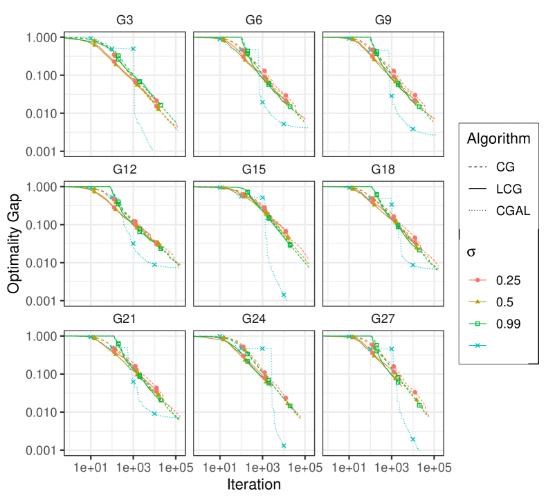
Figure 1: Max-Cut problem: relative gap from SDPT3 solution vs. iteration.

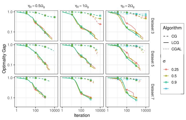
Figure 2: Mixing time problem: relative gap from SDPT3 solution vs. iteration.

5.2 Estimating the mixing time of a Markov chain

Consider a continuous-time Markov chain on a weighted graph, with edge weights representing the transition rates of the process. Let ${\mathbf{P}}(t)=e^{-Lt}$ be the stochastic semi-group of the process, where $L$ is the graph Laplacian. From $L\mathbf{1}=0$ it follows that $\frac{1}{n}\mathbf{1}$ is a stationary distribution of the process. From [7] we have the following bound on the total variation distance of the time $t$ distribution of the Markov process and the stationary distribution $\sup_{\pi}\lVert\pi{\mathbf{P}}(t)-\frac{1}{n}\mathbf{1}\rVert_{\text{TV}}\leq\frac{1}{2}\sqrt{n}e^{-\lambda t}.$ The quantity $T_{\text{mix}}=\lambda$ is called the mixing time. The constant $\lambda$ is the second-largest eigenvalue of the graph Laplacian $L$. To bound this eigenvalue, we follow the SDP-strategy laid out in [31], and in some detail described in Section B in the supplementary materials. In the experiments, we generated random connected undirected graphs with $100-800$ nodes and $10^{3}-10^{4}$ edges, and for each edge $\{i,j\}$ in the graph, we generated a random weight uniformly in $[0,1]$. $\operatorname{\texttt{LCG}}$ exhibits the best computational performance both in the number of iterations and in time. Moreover, for all of the datasets, the primal-dual method $\operatorname{CGAL}$ generated solutions that were far from being feasible. Figure 2 illustrates the optimality gap for the generated results by each method (and the dependence of $\operatorname{\texttt{CG}}$ and $\operatorname{\texttt{LCG}}$ on the starting accuracy $\eta_{0}$), $\operatorname{CGAL}$ only appears in the right most graphs.

6 Complexity Analysis

In this section we give a detailed presentation of the analysis of the iteration complexity of Algorithm 2. The analysis for the inexact version of this scheme is similar, but requires some delicate modifications which we present in detail in Appendix A.

6.1 Analysis of procedure $\operatorname{\texttt{CG}}(x^{0},\varepsilon,t)$

Recall $\Omega_{g}:=\max_{x,y\in\operatorname{dom}(g)\cap\mathsf{X}}\lvert g(x)-g(y)\rvert$ and $\mathsf{C}=\operatorname{dom}(F)\cap\mathsf{X}\cap\operatorname{dom}(g)$. The following estimate can be established as in [41, Prop. 3].

Lemma 6.1.

For all $(x,t)\in\mathsf{C}\times(0,\infty)$, we have

$$t^{-1}\mathtt{e}_{t}(x)\leq\nu/t+\operatorname{\mathsf{Gap}}_{t}(x)+\Omega_{g}.$$ (6.1)

Observe that

$$\mathtt{e}_{t}(x) =\lVert s_{t}(x)-x\rVert_{x}=\sqrt{F^{\prime\prime}(x)[s_{t}(x)-x,s_{t}(x)-x]}$$

$$\geq\nu^{-1/2}\lvert F^{\prime}(x)[s_{t}(x)-x]\rvert$$

$$=\frac{t}{\sqrt{\nu}}\lvert\operatorname{\mathsf{Gap}}_{t}(x)-g(x)+g(s_{t}(x))\rvert$$

$$\geq\frac{t}{\sqrt{\nu}}(\operatorname{\mathsf{Gap}}_{t}(x)-\Omega_{g}).$$ (6.2)

6.1.1 Proof of Proposition 3.3

The proof mainly follows the steps of the proof of Theorem 1 in [41]. The main technical challenge in our analysis is taking care of the penalty parameter $t$.

Lemma 6.2.

At iteration $k$ of Algorithm $\operatorname{\texttt{CG}}(x^{0},\eta,t)$ the following hold:

1. If $\operatorname{\mathsf{Gap}}_{t}(x^{k})>\frac{\nu}{t}+\Omega_{g}$, then the function gap $\Delta_{t}(x^{k}_{t})$ decreases at least linearly at this iteration:

   $$\Delta_{t}(x^{k}_{t})\left[1-\frac{1}{5.3(\nu+t\Omega_{g}+t\Delta_{t}(x^{0}))}\right]\geq\Delta_{t}(x^{k+1}_{t}).$$ (6.3)

   The number of iterations at which linear decrease takes place is at most $K_{t}(x^{0}):=\lceil 5.3(\nu+t\Delta_{t}(x^{0}_{t})+t\Omega_{g})\log(10.6t\Delta_{t}(x^{0}))\rceil$ .

2. If $\operatorname{\mathsf{Gap}}_{t}(x^{k})\leq\frac{\nu}{t}+\Omega_{g}$, then

   $$\frac{1}{\Delta_{t}(x^{k+1}_{t})}\geq\frac{1}{\Delta_{t}(x^{k}_{t})}+\frac{t}{12(\nu+t\Omega_{g})^{2}}$$ (6.4)

Before proving this Lemma, let us explain how we use it to estimate the total number of iterations needed by method $\operatorname{\texttt{CG}}(x^{0},\varepsilon,t)$ until the stopping criterion is satisfied. Motivated by the two different regimes worked out in Lemma 6.2, we define the time windows $\mathbb{K}_{I}(t):=\{k\in\mathbb{N}|\operatorname{\mathsf{Gap}}_{t}(x^{k}_{t})>\mathtt{a}_{t}\}$ (phase I) and $\mathbb{K}_{II}(t):=\{k\in\mathbb{N}|\operatorname{\mathsf{Gap}}_{t}(x^{k}_{t})\leq\mathtt{a}_{t}\}$ (phase II) , where $\mathtt{a}_{t}:=\frac{\nu}{t}+\Omega_{g}$. Part 1 of Lemma 6.2 tells us that $\lvert\mathbb{K}_{I}(t)\rvert\leq K_{t}(x^{0})=\lceil 5.3(\nu+t\Delta_{t}(x^{0}_{t})+t\Omega_{g})\log(10.6t\Delta_{t}(x^{0}_{t}))\rceil$. Thus, to upper bound $R_{G}(x^{0},\eta,t)$ we need also to estimate the reduction in terms of the merit function on phase $\mathbb{K}_{II}(t)$ and obtain the corresponding bound on $\lvert\mathbb{K}_{II}(t)\rvert$.

Proof of Lemma 6.2.

Step 1: Assume iteration $k$ is in phase $\mathbb{K}_{I}(t)$. Set $\mathtt{e}^{k}_{t}\equiv\mathtt{e}_{t}(x^{k}_{t})$ and $G^{k}_{t}\equiv\operatorname{\mathsf{Gap}}_{t}(x^{k}_{t})$. Combining the condition $G^{k}_{t}>\frac{\nu}{t}+\Omega_{g}$ of phase $\mathbb{K}_{I}(t)$ with (6.2), we deduce that $\mathtt{e}^{k}_{t}\geq\sqrt{\nu}\geq 1$. This in turn implies $\frac{tG^{k}_{t}}{\mathtt{e}^{k}_{t}(\mathtt{e}^{k}_{t}+tG^{k}_{t})}<\frac{tG^{k}_{t}}{\mathtt{e}^{k}+tG^{k}_{t}}<1$. Hence, at this iteration algorithm $\operatorname{\texttt{CG}}(x^{0},\varepsilon,t)$ chooses the step sizes $\alpha_{k}=\frac{tG^{k}_{t}}{\mathtt{e}^{k}_{t}(\mathtt{e}^{k}_{t}+tG^{k}_{t})}$. The per-iteration reduction of the potential function can be estimated as follows:

$$V_{t}(x^{k+1}_{t}) \leq V_{t}(x^{k}_{t})-\frac{G^{k}_{t}}{\mathtt{e}^{k}_{t}}\frac{tG^{k}_{t}}{\mathtt{e}_{t}^{k}+tG^{k}_{t}}+\frac{1}{t}\omega_{\ast}\left(\frac{tG^{k}_{t}}{\mathtt{e}_{t}^{k}+tG^{k}_{t}}\right)$$

$$=V_{t}(x^{k}_{t})-\frac{G^{k}_{t}}{\mathtt{e}^{k}_{t}}+\frac{1}{t}\log\left(1+\frac{tG_{t}^{k}}{\mathtt{e}^{k}_{t}}\right)$$

$$=V_{t}(x^{k}_{t})-\frac{1}{t}\omega\left(\frac{tG^{k}_{t}}{\mathtt{e}^{k}_{t}}\right),$$ (6.5)

where $\omega(\tau)=\tau-\log(1+\tau)$. This readily yields $\Delta_{t}(x^{k}_{t})-\Delta_{t}(x^{k+1}_{t})\geq\frac{1}{t}\omega\left(\frac{tG^{k}_{t}}{\mathtt{e}^{k}_{t}}\right)$ and implies that $\{\Delta_{t}(x^{k}_{t})\}_{k\in\mathbb{K}_{I}(t)}$ is monotonically decreasing. For $k\in\mathbb{K}_{I}(t)$, we also see $\frac{tG^{k}_{t}}{\nu+tG^{k}_{t}+t\Omega_{g}}>\frac{1}{2}$. Together with (6.1), this implies

$$\frac{tG_{t}^{k}}{\mathtt{e}^{k}_{t}}\geq\frac{G^{k}_{t}}{\nu/t+G_{t}^{k}+\Omega_{g}}=\frac{tG^{k}_{t}}{\nu+tG_{t}^{k}+t\Omega_{g}}>\frac{1}{2}.$$

Using (3.5), the monotonicity of $\omega(\cdot)$ and that $\omega(\tau)\geq\frac{\tau}{5.3}$ for $\tau\geq 1/2$ (see [41, Prop. 1]), the fact that the function $x\mapsto\frac{x}{a+tx}$ is strictly increasing for $t,a>0$, we arrive at

$$\Delta_{t}(x^{k}_{t})-\Delta_{t}(x^{k+1}_{t})\geq\frac{1}{5.3}\frac{G^{k}_{t}}{\nu+tG^{k}_{t}+t\Omega_{g}}\geq\frac{\Delta_{t}(x^{k}_{t})}{5.3(\nu+t\Omega_{g}+t\Delta_{t}(x^{k}_{t}))}.$$

Coupled with $\Delta_{t}(x^{k}_{t})\leq\Delta_{t}(x^{0}_{t}$), we conclude

$$\Delta_{t}(x^{k}_{t})\left[1-\frac{1}{5.3(\nu+t\Omega_{g}+t\Delta_{t}(x^{0}_{t}))}\right]\geq\Delta_{t}(x^{k+1}_{t}).$$

Define $q_{t}:=\frac{1}{5.3(\nu+t\Omega_{g}+t\Delta_{t}(x^{0}_{t}))}\in(0,1)$ (since $\nu\geq 1$), to arrive at the recursion

$$\Delta_{t}(x^{k}_{t})\leq(1-q_{t})^{k}\Delta_{t}(x^{0}_{t})\leq\exp(-q_{t}k)\Delta_{t}(x^{0}_{t}).$$

Furthermore,

$$\Delta_{t}(x^{k}_{t}) \geq\Delta_{t}(x^{k}_{t})-\Delta_{t}(x^{k+1}_{t})\geq\frac{G_{t}^{k}}{5.3(\nu+tG^{k}_{t}+t\Omega_{g})}\geq\frac{1}{10.6t}.$$

Hence, $\frac{1}{10.6t\Delta_{t}(x^{0}_{t})}\leq\exp(-q_{t}k)$, so that $K_{t}(x^{0}_{t}):=\lceil 5.3(\nu+t\Delta_{t}(x^{0}_{t})+t\Omega_{g})\log(10.6t\Delta_{t}(x^{0}_{t}))\rceil$ defines an upper bound for the cardinality of the set $\mathbb{K}_{I}(t)$. This proves Part 1 of Lemma 6.2.

Step 2: Assume that at iteration $k$ we have $G^{k}_{t}\leq\mathtt{a}_{t}$. We have to distinguish the iterates using large steps $(\alpha_{k}=1$), from those using short steps ($\alpha_{k}<1$).

Let us first consider the case where $\alpha_{k}=1$. Then, $tG^{k}_{t}\geq\mathtt{e}^{k}_{t}(tG^{k}_{t}+\mathtt{e}^{k}_{t})$, which implies $\mathtt{e}^{k}_{t}\in(0,1)$, and $G^{k}_{t}\geq\frac{(\mathtt{e}^{k}_{t})^{2}}{t(1-\mathtt{e}^{k}_{t})}$. Moreover, using (2.7), we readily obtain

$$V_{t}(x^{k+1}_{t}) \leq V_{t}(x^{k}_{t})-G^{k}_{t}+\frac{1}{t}\omega_{\ast}(\mathtt{e}^{k}_{t})$$

$$\leq V_{t}(x^{k}_{t})-G^{k}_{t}+\frac{1}{t}\frac{(\mathtt{e}^{k}_{t})^{2}}{2(1-\mathtt{e}^{k}_{t})}$$

$$\leq V_{t}(x^{k}_{t})-\frac{G_{t}^{k}}{2}.$$

Therefore,

$$\Delta_{t}(x^{k}_{t})-\Delta_{t}(x^{k+1}_{t}) \geq\frac{G_{t}^{k}}{2}\geq\frac{1}{2}\frac{(G_{t}^{k})^{2}}{\nu/t+\Omega_{g}}=\frac{1}{2}\frac{t(G^{k}_{t})^{2}}{\nu+t\Omega_{g}}$$

$$\geq\frac{1}{12}\frac{t(G^{k}_{t})^{2}}{(\nu+t\Omega_{g})^{2}}.$$

In the regime where $\alpha_{k}<1$, we obtain the estimate $\Delta_{t}(x^{k}_{t})-\Delta_{t}(x^{k+1}_{t})\geq\frac{1}{12}\frac{t(G^{k}_{t})^{2}}{(\nu+t\Omega_{g})^{2}}$, by following the same reasoning as in [41]. Using the relation $G^{k}_{t}\geq\Delta_{t}(x^{k}_{t})\geq\Delta_{t}(x^{k+1}_{t})$, we conclude

$$\frac{1}{\Delta_{t}(x^{k+1}_{t})}-\frac{1}{\Delta_{t}(x^{k}_{t})}\geq\frac{t}{12(\nu+t\Omega_{g})^{2}}.$$ (6.6)

$\blacksquare$

Given the pair $(t,\eta)\in(0,\infty)^{2}$, denote by $N\equiv N(x^{0}_{t},\eta,t)$ the upper bound in the r.h.s. of (3.8). We know that at most $K\equiv K_{t}(x^{0}_{t})$ of these iterations are in phase I. Then, from the expression for $N$ in (3.8), we see that at least $M=N-K=\lceil 12(\nu+t\Omega_{g})^{2}(\frac{1}{t\eta}-\frac{1}{t\Delta_{t}(x^{0}_{t})})^{+}\rceil$ iterations belong to phase II. Telescoping the inequality (6.6), we get

$$\frac{1}{\Delta_{t}(x^{N}_{t})}\geq\frac{1}{\Delta_{t}(x^{K}_{t})}+\frac{Mt}{12(\nu+t\Omega_{g})^{2}}\geq\frac{1}{\Delta_{t}(x^{0}_{t})}+\frac{Mt}{12(\nu+t\Omega_{g})^{2}}.$$

Substituting the expression for $M$ ensures that $\Delta_{t}(x^{N}_{t})\leq\eta$. This proves that at most $N$ iterations of $\operatorname{\texttt{CG}}(x^{0}_{t},\eta,t)$ is sufficient for the latter guarantee and finishes the proof.

6.1.2 Proof of Proposition 3.2

Let $\{k_{j}(t)\}_{j}$ denote the increasing set of indices enumerating $\mathbb{K}_{II}(t)$. From the analysis of the trajectory given in the previous section, we know that

$$\Delta_{t}(x_{t}^{k_{j+1}(t)})-\Delta_{t}(x^{k_{j}(t)}_{t})\leq-\frac{1}{12}\frac{t(G_{t}^{k_{j}(t)})^{2}}{(\nu+t\Omega_{g})^{2}},\text{ and }G_{t}^{k_{j}(t)}\geq\Delta_{t}(x^{k_{j}(t)}_{t}).$$

Set $d_{j}\equiv\Delta_{t}(x^{k_{j}(t)}_{t})$ and $\frac{1}{M}\equiv\frac{t}{12(\nu+t\Omega_{g})^{2}},\Gamma_{j}\equiv G_{t}^{k_{j}(t)}$. We thus obtain the recursion

$$d_{j+1}\leq d_{j}-\frac{\Gamma_{j}^{2}}{M},\quad\Gamma_{j}\geq d_{j},$$

and we can apply [41, Prop. 2.4] directly to the above recursion to obtain the estimates

$$d_{j}\leq\frac{M}{j},\quad\text{ and }\min\{\Gamma_{0},\ldots,\Gamma_{j}\}\leq\frac{2M}{j}.$$

Therefore, in order to reach an iterate with $\Gamma_{j}=\operatorname{\mathsf{Gap}}_{t}(x^{k_{j}(t)}_{t})\leq\eta$, it is sufficient to run the process until the label $j$ is reached satisfying $\frac{2M}{j}\leq\eta$. Solving this for $j$ yields $j=\lceil\frac{24(\nu+t\Omega_{g})^{2}}{t\eta}\rceil$. Combined with the upper bound obtained for the time $K_{t}(x^{0}_{t})$ the process spends in phase I, we obtain the total complexity estimate postulated in Proposition 3.2.

6.2 Analysis of the outer loop and proof of Theorem 3.4

Let $I\equiv I(\eta_{0},\sigma,\varepsilon)=\lceil\frac{\log(2\eta_{0}/\varepsilon)}{\log(1/\sigma)}\rceil$ denote the a-priori fixed number of updates of the accuracy and homotopy parameter. We set $\hat{x}_{i}\equiv x^{R_{i}}_{t_{i}}$, the last iterate of procedure $\operatorname{\texttt{CG}}(x^{0}_{t_{i}},\eta_{i},t_{i})$ satisfying $\Delta_{t_{i}}(\hat{x}_{i})\leq\operatorname{\mathsf{Gap}}_{t_{i}}(\hat{x}_{i})\leq\eta_{i}$. From this, using the definition of the gap function, we deduce that

$$g(\hat{x}_{i})-g(z^{\ast}(t_{i}))\leq\operatorname{\mathsf{Gap}}_{t_{i}}(\hat{x}_{i})+\frac{1}{t_{i}}F^{\prime}(\hat{x}_{i})[z^{\ast}(t_{i})-\hat{x}_{i}]\leq\eta_{i}+\frac{\nu}{t_{i}}.$$ (6.7)

Hence, using Lemma 2.2, we observe

$$g(\hat{x}_{i})-\operatorname{Opt}=g(\hat{x}_{i})-g(z^{\ast}(t_{i}))+g(z^{\ast}(t_{i}))-\operatorname{Opt}\leq\eta_{i}+\frac{2\nu}{t_{i}}.$$ (6.8)

Since $t_{i}=\frac{2\nu}{\eta_{i}}$, we obtain $g(\hat{x}_{i})-\operatorname{Opt}\leq 2\eta_{i}$. We next estimate the initial gap $\Delta_{t_{i+1}}(x^{0}_{t_{i+1}})=\Delta_{t_{i+1}}(\hat{x}_{i})$ incurred by our warm-start strategy. Observe that

$$V_{t_{i+1}}(x^{0}_{t_{i+1}})-V_{t_{i+1}}(z^{\ast}(t_{i+1})) =V_{t_{i}}(x^{0}_{t_{i+1}})-V_{t_{i}}(z^{\ast}(t_{i+1}))$$

$$+\left(\frac{1}{t_{i+1}}-\frac{1}{t_{i}}\right)(F(x^{0}_{t_{i+1}})-F(z^{\ast}(t_{i+1})))$$

$$\leq V_{t_{i}}(x^{R_{i}}_{t_{i}})-V_{t_{i}}(z^{\ast}(t_{i}))$$

$$+\left(1-\frac{t_{i+1}}{t_{i}}\right)\left(V_{t_{i+1}}(x^{0}_{t_{i+1}})-V_{t_{i+1}}(z^{\ast}(t_{i+1}))\right)$$

$$+(1-\frac{t_{i+1}}{t_{i}})(g(z^{\ast}(t_{i+1}))-g(x^{0}_{t_{i+1}})).$$

Moreover,

$$g(x^{0}_{t_{i+1}})-g(z^{\ast}(t_{i+1}))\leq g(x^{0}_{t_{i+1}})-\operatorname{Opt}\leq\eta_{i}+\frac{2\nu}{t_{i}}=\frac{4\nu}{t_{i}}.$$

Since $t_{i+1}>t_{i}$, the above two inequalities imply

$$\frac{t_{i+1}}{t_{i}}[V_{t_{i+1}}(x^{0}_{t_{i+1}})-V_{t_{i+1}}(z^{\ast}(t_{i+1}))]\leq V_{t_{i}}(x^{R_{i}}_{t_{i}})-V_{t_{i}}(z^{\ast}(t_{i}))+\frac{t_{i+1}-{t_{i}}}{t_{i}^{2}}4\nu.$$

Whence,

$$t_{i+1}\Delta_{t_{i+1}}(x^{0}_{t_{i+1}})\leq t_{i}\Delta_{t_{i}}(x^{R_{i}}_{t_{i}})+\frac{t_{i+1}-{t_{i}}}{t_{i}}4\nu\leq t_{i}\eta_{i}+\frac{t_{i+1}-{t_{i}}}{t_{i}}4\nu=\left(2\frac{t_{i+1}}{t_{i}}-1\right)2\nu.$$ (6.9)

We are now in the position to estimate the total iteration complexity $\texttt{Compl}(x^{0},\varepsilon,f):=\sum_{i=0}^{I}R_{i}\leq\sum_{i=0}^{I}R_{G}(x^{0}_{t_{i}},\eta_{i},t_{i})$ by using Proposition 3.2, and thereby prove Theorem 3.4. We do so by using the updating regime of the sequences $\{t_{i}\}$ and $\{\eta_{i}\}$ explained in Section LABEL:sec:alg. These updating mechanisms imply

$$\sum_{i=1}^{I}R_{i} \leq\sum_{i=1}^{I}5.3\left(\nu+2\nu\left(\frac{2t_{i}}{t_{i-1}}-1\right)+t_{i}\Omega_{g}\right)\log\left(10.6\left(2\nu\left(\frac{2t_{i}}{t_{i-1}}-1\right)\right)\right)$$

$$+\sum_{i=1}^{I}\frac{12}{\nu}(\nu+t_{i}\Omega_{g})^{2}$$

$$\leq\log(21.2(\nu(2/\sigma-1)))\sum_{i=1}^{I}5.3(\nu(4/\sigma-1)+t_{i}\Omega_{g}))+\sum_{i=1}^{I}\frac{24}{\nu}(\nu^{2}+t^{2}_{i}\Omega^{2}_{g})$$

$$\leq{24}{\nu}\times I+21.2\nu/\sigma\log(42.4\nu/\sigma){\color[rgb]{0,0,0}\times I}+{\color[rgb]{0,0,0}5.3}\log(42.4\nu/\sigma)\Omega_{g}\sum_{i=1}^{I}t_{i}+\frac{24\Omega_{g}^{2}}{\nu}\sum_{i=1}^{I}t_{i}^{2}$$

$$\leq{\color[rgb]{0,0,0}\frac{24\nu\log(2\eta_{0}/\varepsilon)}{\log(1/\sigma)}}+\log\left(\frac{42.4\nu}{\sigma}\right)\frac{21.2\nu}{\sigma}{\color[rgb]{0,0,0}\frac{\log(2\eta_{0}/\varepsilon)}{\log(1/\sigma)}}$$

$$+\log\left(\frac{42.4\nu}{\sigma}\right)\frac{{\color[rgb]{0,0,0}21.2}\nu\Omega_{g}}{\varepsilon(1-\sigma)}+\frac{384\Omega_{g}^{2}\nu}{\varepsilon^{2}(1-\sigma^{2})}.$$

In deriving these bounds, we have used the following estimates:

$$\sum_{i=1}^{I}t_{i}=t_{0}\sigma^{-1}\sum_{i=0}^{I-1}(1/\sigma)^{i}\leq t_{0}\frac{\sigma^{-I}}{1-\sigma}\leq\frac{4\nu}{\varepsilon(1-\sigma)},$$

and

$$\sum_{i=1}^{I}t_{i}^{2}=t^{2}_{0}\sum_{i=1}^{I}(1/\sigma)^{2i}=\frac{t^{2}_{0}}{\sigma^{2}}\sum_{i=0}^{I-1}(1/\sigma^{2})^{i}\leq\frac{16\nu^{2}}{\varepsilon^{2}(1-\sigma^{2})}.$$

It remains to bound the complexity at $i=0$. We have

$$R_{0} \leq 5.3(\nu+t_{0}\Delta_{t_{0}}(x^{0}_{t_{0}})+t_{0}\Omega_{g})\log(10.6t_{0}\Delta_{t_{0}}(x^{0}))+\frac{12}{\nu}(\nu+t_{0}\Omega_{g})^{2}$$

$$\leq 5.3(\nu+F(x^{0})-F(z^{\ast}(t_{0}))+2t_{0}\Omega_{g})\log\left(10.6(F(x^{0})-F(z^{\ast}(t_{0}))+t_{0}\Omega_{g})\right)$$

$$+\frac{24}{\nu}(\nu^{2}+t^{2}_{0}\Omega^{2}_{g}).$$

Since $t_{0}=\frac{\nu}{\Omega_{g}}$ and $\eta_{0}=2\Omega_{g}$, we have

$$R_{0}\leq 5.3(3\nu+F(x^{0})-F(z^{\ast}(t_{0})))\log\left(10.6(\nu+F(x^{0})-F(z^{\ast}(t_{0})))\right)+48\nu.$$

Adding the two gives the total complexity bound

$$\texttt{Compl}(x^{0},\varepsilon,f) \leq 5.3(3\nu+F(x^{0})-F(z^{\ast}(t_{0})))\log\left(10.6(\nu+F(x^{0})-F(z^{\ast}(t_{0})))\right)+48\nu$$

$$+\frac{\nu\log(2\eta_{0}/\varepsilon)}{\log(1/\sigma)}\left[24+\log\left(\frac{42.4\nu}{\sigma}\right)\frac{21.2\nu}{\sigma}\right]$$

$$+\log\left(\frac{42.4\nu}{\sigma}\right)\frac{21.2\nu\Omega_{g}}{\varepsilon(1-\sigma)}+\frac{384\Omega_{g}^{2}\nu}{\varepsilon^{2}(1-\sigma^{2})}.$$

$$=O\left(\frac{\Omega_{g}^{2}\nu}{\varepsilon^{2}(1-\sigma^{2})}\right).$$

7 Conclusions

Solving large scale conic-constrained convex programming problems is still a key challenge in mathematical optimization and machine learning. In particular, SDPs with a massive amount of linear constraints appear naturally as convex relaxations of combinatorial optimization problems. For such problems, the development of scalable algorithms is a very active field of research [39, 12]. In this paper, we propose a new path-following/homotopy strategy to solve such massive conic-constrained problems, building on recent advances in projection-free methods for self-concordant minimization [41, 9, 11]. Our scheme possesses favorable theoretical iteration complexity and gives promising results in practice. Future work will focus on improvements of our deployed CndG solver to accelerate the subroutines.

Appendix A Modifications Due to Inexact Oracles

In this appendix we give the missing proofs of the theoretical statements in Sections 3.5 and 3.6. Consider the function $\tilde{\mathtt{e}}_{t}(x):=\lVert\tilde{s}_{t}(x)-x\rVert_{x}$, where $\tilde{s}_{t}(x)$ is any member of the set $\mathcal{L}^{(\delta,\theta)}_{g}(\frac{1}{t}\nabla F(x))$ (cf. Definition 3.5). It is easy to see that Lemma 6.1 translates to the case with inexact oracle feedback as

$$t^{-1}\tilde{\mathtt{e}}_{t}(x)\leq\nu/t+\widetilde{\operatorname{\mathsf{Gap}}}_{t}(x)+\Omega_{g}.$$ (A.1)

Moreover, one can show that

$$\tilde{\mathtt{e}}_{t}(x)\geq\frac{t}{\sqrt{\nu}}\lvert\widetilde{\operatorname{\mathsf{Gap}}}_{t}(x)-\Omega_{g}\rvert.$$ (A.2)

A.1 Proof of Proposition 3.7

The proof of this proposition mimics the proof of the exact regime (cf. Proposition 3.3), with some important twists. We split the analysis into two phases, bound the maximum number of iterations the algorithms can spend on these phases, and add these numbers up to obtain the worst-case upper bound.

First, for a round $k$ of $\texttt{ICG}(x,t,\eta,\delta,\theta)$, we use the abbreviations

$$\tilde{s}_{t}^{k}=\tilde{s}_{t}(x^{k}_{t}),\;\tilde{\mathtt{e}}_{t}^{k}\equiv\lVert\tilde{s}_{t}^{k}-x^{k}_{t}\rVert_{x^{k}_{t}},\;\tilde{G}^{k}_{t}\equiv\widetilde{\operatorname{\mathsf{Gap}}}_{t}(x^{k}_{t}),\;\tilde{\alpha}_{t}^{k}\equiv\tilde{\alpha}_{t}(x^{k}_{t}).$$

We further redefine the phases as $\mathbb{K}_{I}(t):=\{k\in\mathbb{N}|\widetilde{\operatorname{\mathsf{Gap}}}_{t}(x^{k}_{t})>\mathtt{a}_{t}\}$ (phase I) and $\mathbb{K}_{II}(t):=\{k\in\mathbb{N}|\widetilde{\operatorname{\mathsf{Gap}}}_{t}(x^{k}_{t})\leq\mathtt{a}_{t}\}$ (phase II), where $\mathtt{a}_{t}:=\frac{\nu}{t}+\Omega_{g}$.

Note that in the analysis we use the inequality $\Delta_{t}(x^{k}_{t})>\eta+\theta$ since our goal is to estimate the number of iterations to achieve $\Delta_{t}(x^{k}_{t})\leq\eta+\theta$. Moreover, if the stopping condition $\widetilde{\operatorname{\mathsf{Gap}}}_{t}(x^{k}_{t})\equiv\tilde{G}^{k}_{t}\leq\eta\delta$ holds, we obtain by the definition of the ILMO and inequality (3.5) that

$$\eta\delta\geq\widetilde{\operatorname{\mathsf{Gap}}}_{t}(x^{k}_{t})\geq\delta(\operatorname{\mathsf{Gap}}_{t}(x^{k}_{t})-\theta)\geq\delta(\Delta_{t}(x^{k}_{t})-\theta),$$ (A.3)

which implies that $\Delta_{t}(x^{k}_{t})\leq\eta+\theta$. Thus, in the analysis we also use the inequality $\tilde{G}^{k}_{t}>\eta\delta>0$.

Analysis for Phase I

Consider $k\in\mathbb{K}_{I}(t)$. Combining the condition $\tilde{G}^{k}_{t}>\frac{\nu}{t}+\Omega_{g}$ of this phase with (A.2), we deduce that $\tilde{\mathtt{e}}^{k}_{t}\geq\sqrt{\nu}\geq 1$. This in turn implies $\frac{t\tilde{G}^{k}_{t}}{\tilde{\mathtt{e}}^{k}_{t}(\tilde{\mathtt{e}}^{k}_{t}+t\tilde{G}^{k}_{t})}<\frac{t\tilde{G}^{k}_{t}}{\tilde{\mathtt{e}}^{k}+t\tilde{G}^{k}_{t}}<1$. Hence, at this iteration algorithm $\texttt{ICG}(x,t,\eta,\delta,\theta)$ chooses the step size $\tilde{\alpha}_{t}^{k}=\frac{t\tilde{G}^{k}_{t}}{\tilde{\mathtt{e}}^{k}_{t}(\tilde{\tilde{\mathtt{e}}}^{k}_{t}+t\tilde{G}^{k}_{t})}$. The per-iteration reduction of the potential function can then be estimated just as in the derivation of (6.5):

$$V_{t}(x^{k+1}_{t})\leq V_{t}(x^{k}_{t})-\frac{1}{t}\omega\left(\frac{t\tilde{G}^{k}_{t}}{\tilde{\mathtt{e}}_{t}^{k}}\right).$$ (A.4)

Note that the r.h.s. is well-defined since $\tilde{G}^{k}_{t}>\eta\delta>0$ as the stopping condition is not yet achieved. The above inequality, using the definition of the potential function gap as $\Delta_{t}(x^{k}_{t})=V_{t}(x^{k}_{t})-V_{t}(z^{\ast}(t))$, readily yields $\Delta_{t}(x^{k}_{t})-\Delta_{t}(x^{k+1}_{t})\geq\frac{1}{t}\omega\left(\frac{t\tilde{G}^{k}_{t}}{\tilde{\mathtt{e}}^{k}_{t}}\right)$ and, in turn, that $\{\Delta_{t}(x^{k}_{t})\}_{k\in\mathbb{K}_{I}(t)}$ is monotonically decreasing.

Since $k\in\mathbb{K}_{I}(t)$, we have that $\frac{t\tilde{G}^{k}_{t}}{\nu+t\tilde{G}^{k}_{t}+t\Omega_{g}}>\frac{1}{2}$. Together with (A.1), this implies

$$\frac{t\tilde{G}_{t}^{k}}{\tilde{\mathtt{e}}^{k}_{t}}\geq\frac{\tilde{G}^{k}_{t}}{\nu/t+\tilde{G}_{t}^{k}+\Omega_{g}}=\frac{t\tilde{G}^{k}_{t}}{\nu+t\tilde{G}_{t}^{k}+t\Omega_{g}}>\frac{1}{2}.$$

Using the monotonicity of $\omega(\cdot)$ and that $\omega(\tau)\geq\frac{\tau}{5.3}$ for $\tau\geq 1/2$ (see [41, Prop. 1]), we further obtain

$$\Delta_{t}(x^{k}_{t})-\Delta_{t}(x^{k+1}_{t})\geq\frac{1}{t}\omega\left(\frac{t\tilde{G}^{k}_{t}}{\tilde{\mathtt{e}}^{k}_{t}}\right)\geq\frac{\tilde{G}^{k}_{t}}{5.3(\nu+t\Omega_{g}+t\tilde{G}_{t}^{k})}.$$ (A.5)

By our definition of the inexact oracle, inequalities (3.5) and $\Delta_{t}(x^{k}_{t})>\eta+\theta$, we see that

$$\tilde{G}^{k}_{t}\equiv\widetilde{\operatorname{\mathsf{Gap}}}_{t}(x^{k}_{t})\geq\delta(\operatorname{\mathsf{Gap}}_{t}(x^{k}_{t})-\theta)\geq\delta(\Delta_{t}(x^{k}_{t})-\theta)>\eta>0.$$

Combining this, (A.5), and the fact that the function $x\mapsto\frac{x}{a+tx}$ is strictly increasing for $a,t>0$ and $x>0$, we obtain

$$\Delta_{t}(x^{k}_{t})-\Delta_{t}(x^{k+1}_{t})\geq\frac{\delta(\Delta_{t}(x^{k}_{t})-\theta)}{5.3[t\delta(\Delta_{t}(x^{k}_{t})-\theta)+\nu+t\Omega_{g}]}\geq\frac{\delta(\Delta_{t}(x^{k}_{t})-\theta)}{5.3[t\delta(\Delta_{t}(x^{0}_{t})-\theta)+\nu+t\Omega_{g}]},$$ (A.6)

where in the last inequality we used that $\Delta_{t}(x^{k}_{t})>\eta+\theta\geq\theta$ and the monotonicity of $\{\Delta_{t}(x^{k}_{t})\}_{k\in\mathbb{K}_{I}(t)}$.

Rearranging the terms and defining $q:=\frac{\delta}{5.3(t\delta(\Delta_{t}(x^{0}_{t})-\theta)+\nu+t\Omega_{g})}$, which we know to be in $(0,1)$ since $\nu\geq 1$ and $\Delta_{t}(x^{0}_{t})>\eta+\theta$, it follows from the previous display that

$$\Delta_{t}(x^{k+1}_{t})\leq\Delta_{t}(x^{k}_{t})(1-q)+q\theta\leq\Delta_{t}(x^{0}_{t})(1-q)^{k}+\theta\leq\exp(-kq)\Delta_{t}(x^{0}_{t})+\theta.$$ (A.7)

On the other hand, we have

$$\Delta_{t}(x^{k}_{t})\geq\Delta_{t}(x^{k}_{t})-\Delta_{t}(x^{k+1}_{t})\geq\frac{\tilde{G}^{k}_{t}}{5.3(\nu+t\Omega_{g}+t\tilde{G}_{t}^{k})}>\frac{1}{10.6t}$$

since $\frac{t\tilde{G}^{k}_{t}}{\nu+t\tilde{G}^{k}_{t}+t\Omega_{g}}>\frac{1}{2}$ for $k\in\mathbb{K}_{I}(t)$. Moreover, we know that $\Delta_{t}(x^{k}_{t})>\eta+\theta$, which gives us in combination with (A.7)

$$\max\left\{\frac{1}{10.6t},\eta+\theta\right\}\leq\Delta_{t}(x^{k}_{t})\leq\exp(-kq)\Delta_{t}(x^{0}_{t})+\theta.$$ (A.8)

Solving w.r.t. $k$, we see that the number of iterations $k\in\mathbb{K}_{I}(t)$ is bounded as

$$K_{t}(x_{t}^{0})=\left\lceil\frac{5.3(t\delta(\Delta_{t}(x^{0}_{t})-\theta)+\nu+t\Omega_{g})}{\delta}\log\left(\min\left\{\frac{10.6t\Delta_{t}(x^{0}_{t})}{(1-10.6t\theta)_{+}},\frac{\Delta_{t}(x^{0}_{t})}{\eta}\right\}\right)\right\rceil.$$ (A.9)

Analysis for Phase II

Consider $k\in\mathbb{K}_{II}(t)$, which means that $\tilde{G}_{t}^{k}\leq\frac{\nu}{t}+\Omega_{g}$. There are two cases we need to consider depending on the stepsize $\tilde{\alpha}_{t}^{k}$.

First, assume that $\tilde{\alpha}_{t}^{k}=1$. Then $t\tilde{G}_{t}^{k}\geq\tilde{\mathtt{e}}^{k}_{t}(\tilde{\mathtt{e}}_{t}^{k}+t\tilde{G}_{t}^{k})$, which implies $\tilde{\mathtt{e}}_{t}^{k}\in(0,1)$. From there we conclude that $\tilde{G}_{t}^{k}\geq\frac{(\tilde{\mathtt{e}}_{t}^{k})^{2}}{t(1-\tilde{\mathtt{e}}_{t}^{k})}$, and, by (3.6) and (2.7), that

$$V_{t}(x^{k+1}_{t}) \leq V_{t}(x^{k}_{t})-\tilde{G}_{t}^{k}+\frac{1}{t}\omega_{\ast}(\tilde{\mathtt{e}}_{t}^{k})$$

$$\leq V_{t}(x^{k}_{t})-\tilde{G}_{t}^{k}+\frac{1}{t}\frac{(\tilde{\mathtt{e}}^{k}_{t})^{2}}{2(1-\tilde{\mathtt{e}}_{t}^{k})}$$

$$\leq V_{t}(x^{k}_{t})-\frac{\tilde{G}^{k}_{t}}{2}.$$

Therefore, using again that $\tilde{G}_{t}^{k}\leq\frac{\nu}{t}+\Omega_{g}$, we have

$$\Delta_{t}(x^{k}_{t})-\Delta_{t}(x^{k+1}_{t})\geq\frac{\tilde{G}^{k}_{t}}{2}\geq\frac{(\tilde{G}^{k}_{t})^{2}}{2(\nu/t+\Omega_{g})}\geq\frac{t(\tilde{G}^{k}_{t})^{2}}{12(\nu+t\Omega_{g})^{2}}.$$ (A.10)

In particular, we see again that $\Delta_{t}(x^{k}_{t})$ is monotonically decreasing since $\tilde{G}^{k}_{t}>\eta\delta>0$.

Consider now the case where $\tilde{\alpha}_{t}^{k}<1$, i.e., $\tilde{\alpha}_{k}=\frac{t\tilde{G}^{k}_{t}}{\tilde{\mathtt{e}}^{k}_{t}(\tilde{\mathtt{e}}^{k}_{t}+t\tilde{G}^{k}_{t})}$. Then, using this stepsize, just as in the derivation of (6.5) and (A.4), we get

$$V_{t}(x^{k+1}_{t})\leq V_{t}(x^{k}_{t})-\frac{1}{t}\omega\left(\frac{t\tilde{G}^{k}_{t}}{\tilde{\mathtt{e}}_{t}^{k}}\right).$$ (A.11)

Again, since $\tilde{G}_{t}^{k}\leq\frac{\nu}{t}+\Omega_{g}$ for $k\in\mathbb{K}_{II}(t)$, we have $\frac{\tilde{G}^{k}_{t}}{\tilde{G}^{k}_{t}+\nu/t+\Omega_{g}}\leq\frac{1}{2}$. Using the monotonicity of $\omega(\tau)$, inequality (A.1), and that $\omega(\tau)\geq\frac{\tau^{2}}{3}$ for $\tau\leq 1/2$ (see [41, Prop. 1]), we can develop the bound

$$\frac{1}{t}\omega\left(\frac{t\tilde{G}^{k}_{t}}{\tilde{\mathtt{e}}_{t}^{k}}\right)=\frac{1}{t}\omega\left(\frac{\tilde{G}^{k}_{t}}{\tilde{\mathtt{e}}_{t}^{k}/t}\right)\geq\frac{1}{t}\omega\left(\frac{\tilde{G}^{k}_{t}}{\tilde{G}^{k}_{t}+\nu/t+\Omega_{g}}\right)\geq\frac{1}{3t}\left(\frac{\tilde{G}^{k}_{t}}{\tilde{G}^{k}_{t}+\nu/t+\Omega_{g}}\right)^{2}.$$

This and (A.11), again by $\tilde{G}_{t}^{k}\leq\frac{\nu}{t}+\Omega_{g}$, implies that also in this regime we obtain the estimate

$$\Delta_{t}(x^{k}_{t})-\Delta_{t}(x^{k+1}_{t})\geq\frac{t(\tilde{G}^{k}_{t})^{2}}{12(\nu+t\Omega_{g})^{2}}.$$ (A.12)

As we see, the above inequality holds on the whole phase II, both when $\tilde{\alpha}_{t}^{k}<1$ and when $\tilde{\alpha}_{t}^{k}=1$. In particular, since $\tilde{G}^{k}_{t}>\eta\delta>0$, the above inequality implies that the sequence $\{\Delta_{t}(x^{k}_{t})\}_{k\in\mathbb{K}_{II}(t)}$ is monotonically decreasing, which combined with the analysis of phase I means that the whole sequence $\{\Delta_{t}(x^{k}_{t})\}_{k}$ is monotonically decreasing.

Finalizing the proof

Let $K$ denote the number in the r.h.s. of (3.13) and let $\texttt{ICG}(x,t,\eta,\delta,\theta)$ be run for $K$ iterations. Let $N_{t}(x_{t}^{0})=\left\lceil\frac{12(\nu+t\Omega_{g})^{2}}{t\delta^{2}}\left(\frac{1}{\eta}-\frac{1}{\Delta_{t}(x^{0}_{t})-\theta}\right)_{+}\right\rceil$. Then, from the expression for $K$ and the analysis of phase I, we know that at least $N_{t}(x_{t}^{0})+1$ iterations belong to the phase II. If at some of these iterations, we have $\Delta_{t}(x^{k}_{t})\leq\eta+\theta$, the result of the proposition follows. Thus, we assume that for the whole phase II $\Delta_{t}(x^{k}_{t})>\eta+\theta>\theta$. Let $k_{1}(t)<k_{2}(t)<\ldots<k_{N_{t}(x_{t}^{0})+1}(t)$ be an increasing enumeration of the iterates in $\mathbb{K}_{II}(t)$. Then, using the monotonicity of the entire sequence $\{\Delta_{t}(x^{k}_{t})\}_{k}$, calling $\Delta_{t}^{j}\equiv\Delta(x^{k_{j}(t)}_{t})$, we see from (A.12) and (A.3) that, for $j=1,\ldots,N_{t}(x_{t}^{0})$,

$$\Delta^{j}_{t}-\Delta^{j+1}_{t}\geq\Delta^{j}_{t}-\Delta_{t}(x^{k_{j}(t)+1}_{t})\geq\frac{t(\tilde{G}^{k}_{t})^{2}}{12(\nu+t\Omega_{g})^{2}}\geq\frac{t\delta^{2}(\Delta^{j}_{t}-\theta)(\Delta^{j+1}_{t}-\theta)}{12(\nu+t\Omega_{g})^{2}}.$$

This implies since $\Delta_{t}(x^{k}_{t})>\theta$ for $j=1,\ldots,N_{t}(x_{t}^{0})+1$ that

$$\frac{1}{\Delta^{j+1}_{t}-\theta}-\frac{1}{\Delta^{j}_{t}-\theta}\geq\frac{t\delta^{2}}{12(\nu+t\Omega_{g})^{2}},\quad j=1,\ldots,N_{t}(x_{t}^{0}).$$

Telescoping this expression, we see

$$\frac{1}{\Delta^{N_{t}(x_{t}^{0})+1}_{t}-\theta}\geq\frac{N_{t}(x_{t}^{0})t\delta^{2}}{12(\nu+t\Omega_{g})^{2}}+\frac{1}{\Delta_{t}(x_{t}^{0})-\theta}\geq\frac{1}{\eta},$$

which finishes the proof.

A.2 Proof of Proposition 3.6

Our analysis concentrates on the behavior of the algorithm in Phase II since the estimate for number of iterations in Phase I still holds. Here we split the iterates of the set $\mathbb{K}_{II}(t)=\{k_{1}(t),\ldots,k_{p}(t)\}\equiv\{k_{1},\ldots,k_{p}\}$ into two regimes so that $\mathbb{K}_{II}(t)=H_{t}\cup L_{t}$ with $L_{t}:=\{k\in\mathbb{K}_{II}(t)|\Delta_{t}(x^{k}_{t})<\theta\}$ and $H_{t}:=\{k\in\mathbb{K}_{II}(t)|\Delta_{t}(x^{k})\geq\theta\}$. By monotonicity of the potential function gap, we know that the indices of of $H_{t}$ (’high states’) precede those of $L_{t}$ (’low states’). We bound the size of each of these subsets in order to make $\widetilde{\operatorname{\mathsf{Gap}}}_{t}$ smaller than $\eta\delta$. Since the potential function gap is monotonically decreasing, we can organize the iterates on phase II as $H_{t}=\{k_{1},\ldots,k_{q}\}$ and accordingly, $L_{t}=\{k_{q+1},\ldots,k_{p}\}$ for some $q\in\{1,\ldots,p\}$.

Bound of $H_{t}$

For $k_{j}(t)\in H_{t}$ we know that

$$\Delta_{t}(x^{k_{j}(t)}_{t})-\Delta_{t}(x^{k_{j+1}(t)}_{t})\geq\Delta_{t}(x^{k_{j}(t)}_{t})-\Delta_{t}(x^{k_{j}(t)+1}_{t})\geq\frac{t(\tilde{G}^{k_{j}(t)}_{t})^{2}}{12(\nu+t\Omega_{g})^{2}}.$$ (A.13)

Define $d_{j}:=\delta(\Delta_{t}(x^{k_{j}(t)}_{t})-\theta)$ for $j=1,\ldots,q$, so that $d_{j}\geq 0$. Then, we obtain the recursion

$$d_{j+1}-d_{j}\leq-\frac{\Gamma^{2}_{j}}{M}$$

for $j\in\{1,\ldots,q-1\}$ and $\Gamma_{j}\equiv\tilde{G}^{k_{j}(t)}_{t}\geq d_{j}$ and $\frac{1}{M}\equiv\frac{t\delta}{12(\nu+t\Omega_{g})^{2}}$. By [41, Proposition 4], we can conclude that

$$d_{q}<\frac{M}{q-1}\text{ and }\min\{\Gamma_{1},\ldots,\Gamma_{q}\}<\frac{2M}{q-1}.$$

Since we know that $\min\{\Gamma_{1},\ldots,\Gamma_{q}\}\geq\delta\eta$, we obtain the bound

$$q\leq\frac{2M}{\delta\eta}+1=\frac{24(\nu+t\Omega_{g})^{2}}{t\delta^{2}\eta}+1.$$ (A.14)

Bound of $L_{t}$

On this subset we cannot use the same argument as for the iterates in $H_{t}$, since we cannot guarantee that the sequence $d_{j}$ involved in the previous part of the proof is positive. However, we still know that (A.13) applies for the iterates in $L_{t}$. If we telescope this expression over the indices $q+1,\ldots,p$, and using the fact that $\Delta_{t}(x^{k_{j}}(t))\in[0,\theta]$, we see that

$$\theta\geq\Delta_{t}(x_{t}^{k_{q+1}(t)})-\Delta_{t}(x_{t}^{k_{p+1}(t)}) \geq\frac{t(p-q)}{12(\nu+t\Omega_{g})^{2}}\min_{q+1\leq j\leq p}\left(\tilde{G}_{t}^{k_{j}(t)}\right)^{2}$$

$$\geq\frac{t(p-q)\eta^{2}\delta^{2}}{12(\nu+t\Omega_{g})^{2}}$$

It follows

$$(p-q)\leq\frac{12\theta(\nu+t\Omega_{g})^{2}}{t\eta^{2}\delta^{2}}.$$ (A.15)

Combining the branches

Combining the expressions (A.14) and (A.15) together with the bound (A.9) for the length of phase I, we see that

$$R_{\tilde{G},t}(x^{0}_{t},\eta,\delta,\theta) \leq\left\lceil\frac{5.3(t\delta(\Delta_{t}(x^{0}_{t})-\theta)+\nu+t\Omega_{g})}{\delta}\log\left(\min\left\{\frac{10.6t\Delta_{t}(x^{0}_{t})}{(1-10.6t\theta)_{+}},\frac{\Delta_{t}(x^{0}_{t})}{\eta}\right\}\right)\right\rceil$$

$$+\left\lceil\frac{12(\nu+t\Omega_{g})^{2}}{t\delta^{2}\eta}\left(2+\frac{\theta}{\eta}\right)\right\rceil+1$$

A.3 Analysis of the outer loop and proof of Theorem 3.8

We set $\hat{x}_{i}\equiv x^{\tilde{R}_{i}}_{t_{i}}$ the last iterate of procedure $\operatorname{\texttt{ICG}}(x^{0}_{t_{i}},t_{i},\eta_{i},\delta,\theta_{i})$, where $\tilde{R}_{i}$ is at most $R_{\tilde{G},t_{i}}(x^{0}_{t_{i}},\eta_{i},\delta,\theta_{i})$ by Proposition 3.6. Therefore, we know that $\widetilde{\operatorname{\mathsf{Gap}}}_{t_{i}}(\hat{x}_{i})\leq\eta_{i}\delta$, and a-fortiori

$$\Delta_{t_{i}}(\hat{x}_{i})\leq\operatorname{\mathsf{Gap}}_{t_{i}}(\hat{x}_{i})\leq\eta_{i}+\theta_{i}.$$

By eq. Eq. 6.7 and the definition of the $(\delta,\theta_{i})$-ILMO, we obtain

$$g(\hat{x}_{i})-g(z^{\ast}(t_{i})) \leq\operatorname{\mathsf{Gap}}_{t_{i}}(\hat{x}_{i})+\frac{1}{t}F^{\prime}(\hat{x}_{i})[z^{\ast}(t_{i})-\hat{x}_{i}]$$

$$\leq\frac{\widetilde{\operatorname{\mathsf{Gap}}}_{t_{i}}(\hat{x}_{i})}{\delta}+\theta_{i}+\frac{\nu}{t_{i}}$$

$$\leq\eta_{i}+\theta_{i}+\frac{\nu}{t_{i}}.$$

Hence, using Lemma 2.2, we observe

$$g(\hat{x}_{i})-\operatorname{Opt}=g(\hat{x}_{i})-g(z^{\ast}(t_{i}))+g(z^{\ast}(t_{i}))-\operatorname{Opt}\leq\eta_{i}+\theta_{i}+\frac{2\nu}{t_{i}}.$$

Since $t_{i}=\frac{2\nu}{\eta_{i}}$ and $\theta_{i}=\eta_{i}$, we obtain $g(\hat{x}_{i})-\operatorname{Opt}\leq 3\eta_{i}$. The latter, by the choice of the number of restarts $I$ implies that

$$g(\hat{z})-\operatorname{Opt}=g(\hat{x}_{I})-\operatorname{Opt}\leq\varepsilon.$$

Our next goal is to estimate the total number of inner iterations based on the estimation for the first epoch $i=0$ and summation over epochs $i=1,...,I$. For each epoch we use the estimate from Proposition 3.6, which we repeat here for convenience

$$R_{\tilde{G},t_{i}}(x^{0}_{t_{i}},\eta_{i},\delta,\theta_{i}) \leq\left\lceil\frac{5.3(t_{i}\delta(\Delta_{t_{i}}(x^{0}_{i})-\theta_{i})+\nu+t_{i}\Omega_{g})}{\delta}\log\left(\min\left\{\frac{10.6t_{i}\Delta_{t_{i}}(x^{0}_{t_{i}})}{(1-10.6t_{i}\theta_{i})_{+}},\frac{\Delta_{t_{i}}(x^{0}_{t_{i}})}{\eta_{i}}\right\}\right)\right\rceil$$

$$\hskip 16.00003pt+\left\lceil\frac{12(\nu+t_{i}\Omega_{g})^{2}}{t_{i}\delta^{2}\eta_{i}}\left(2+\frac{\theta_{i}}{\eta_{i}}\right)\right\rceil+1.$$ (A.16)

We see that we need to estimate the quantities $t_{i}(\Delta_{t_{i}}(x^{0}_{i})-\theta_{i})$ and $\frac{\Delta_{t_{i}}(x^{0}_{t_{i}})}{\eta_{i}}$, which is our next step. Consider $i\geq 1$ and observe that

$$V_{t_{i+1}}(x^{0}_{t_{i+1}})-V_{t_{i+1}}(z^{\ast}(t_{i+1})) =V_{t_{i}}(x^{0}_{t_{i+1}})-V_{t_{i}}(z^{\ast}(t_{i+1}))$$

$$+\left(\frac{1}{t_{i+1}}-\frac{1}{t_{i}}\right)(F(x^{0}_{t_{i+1}})-F(z^{\ast}(t_{i+1})))$$

$$\leq V_{t_{i}}(x^{R_{i}}_{t_{i}})-V_{t_{i}}(z^{\ast}(t_{i}))$$

$$+\left(1-\frac{t_{i+1}}{t_{i}}\right)\left(V_{t_{i+1}}(x^{0}_{t_{i+1}})-V_{t_{i+1}}(z^{\ast}(t_{i+1}))\right)$$

$$+(1-\frac{t_{i+1}}{t_{i}})(g(z^{\ast}(t_{i+1}))-g(x^{0}_{t_{i+1}})).$$

Moreover,

$$g(x^{0}_{t_{i+1}})-g(z^{\ast}(t_{i+1}))\leq g(x^{0}_{t_{i+1}})-\operatorname{Opt}\leq\eta_{i}+\theta_{i}+\frac{2\nu}{t_{i}}.$$

Since $t_{i+1}>t_{i}$, the above two inequalities imply

$$\frac{t_{i+1}}{t_{i}}[V_{t_{i+1}}(x^{0}_{t_{i+1}})-V_{t_{i+1}}(z^{\ast}(t_{i+1}))]\leq V_{t_{i}}(x^{R_{i}}_{t_{i}})-V_{t_{i}}(z^{\ast}(t_{i}))+\frac{t_{i+1}-{t_{i}}}{t_{i}}(\eta_{i}+\theta_{i}+\frac{2\nu}{t_{i}}).$$

Whence,

$$t_{i+1}(\Delta_{t_{i+1}}(x^{0}_{t_{i+1}})-\theta_{i+1}) \leq t_{i}\Delta_{t_{i}}(x^{R_{i}}_{t_{i}})+(t_{i+1}-t_{i})(\eta_{i}+\theta_{i}+\frac{2\nu}{t_{i}})-t_{i+1}\theta_{i+1}$$

$$\leq t_{i}(\eta_{i}+\theta_{i})+(t_{i+1}-t_{i})(\eta_{i}+\theta_{i}+\frac{2\nu}{t_{i}})-t_{i+1}\theta_{i+1}$$

$$=4\nu+(t_{i+1}-t_{i})\cdot\frac{6\nu}{t_{i}}-2\nu=2\nu+(1/\sigma-1)6\nu=2\nu(3/\sigma-2),$$

where we used our assignments $t_{i+1}=t_{i}/\sigma,\eta_{i}t_{i}=\theta_{i}t_{i}=2\nu$. In the same way, we obtain

$$\frac{\Delta_{t_{i+1}}(x^{0}_{t_{i+1}})}{\eta_{i+1}} \leq\frac{t_{i}}{t_{i+1}\eta_{i+1}}\Delta_{t_{i}}(x^{R_{i}}_{t_{i}})+\frac{t_{i+1}-t_{i}}{t_{i+1}\eta_{i+1}}(\eta_{i}+\theta_{i}+\frac{2\nu}{t_{i}})$$

$$\leq\frac{t_{i}}{t_{i+1}\eta_{i+1}}(\eta_{i}+\theta_{i})+\frac{t_{i+1}-t_{i}}{t_{i+1}\eta_{i+1}}(\eta_{i}+\theta_{i}+\frac{2\nu}{t_{i}})$$

$$=\frac{4\nu}{t_{i+1}\eta_{i+1}}+\frac{t_{i+1}-t_{i}}{t_{i+1}\eta_{i+1}}\frac{6\nu}{t_{i}}=2+(1/\sigma-1)3=(3/\sigma-1),$$

where we again used our assignments $t_{i+1}=t_{i}/\sigma,\eta_{i}t_{i}=\theta_{i}t_{i}=2\nu$.

Using these bounds, our assignments $\eta_{i}=\theta_{i}=2\nu/t_{i}$, we see that $1-10.6t_{i}\theta_{i}<0$ and the bound (A.3) simplifies to

$$R_{\tilde{G},t_{i}}(x^{0}_{t_{i}},\eta_{i},\delta,\theta_{i}) \leq\left\lceil\frac{5.3(2\delta\nu(3/\sigma-2)+\nu+t_{i}\Omega_{g})}{\delta}\log(3/\sigma-1)\right\rceil+\left\lceil\frac{18(\nu+t_{i}\Omega_{g})^{2}}{\nu\delta^{2}}\right\rceil+1$$ (A.17)

$$\leq 3+\frac{5.3(2\delta\nu(3/\sigma-2)+\nu)}{\delta}\log(3/\sigma-1)+\frac{18\nu}{\delta^{2}}$$ (A.18)

$$\hskip 8.00002pt+t_{i}\cdot\left(\frac{5.3\Omega_{g}}{\delta}\log(3/\sigma-1)+\frac{18\Omega_{g}}{\delta^{2}}\right)+t_{i}^{2}\cdot\frac{18\Omega_{g}^{2}}{\nu\delta^{2}}.$$ (A.19)

Using the same bounds for $\sum_{i}t_{i}$, $\sum_{i}t_{i}^{2}$ as in the proof of Theorem 3.4 (see Section 6.2), we obtain that

$$\sum_{i=1}^{I}\tilde{R}_{i} \leq\left(3+\frac{5.3(2\delta\nu(3/\sigma-2)+\nu)}{\delta}\log(3/\sigma-1)+\frac{18\nu}{\delta^{2}}\right)\frac{\log(2\eta_{0}/\varepsilon)}{\log(1/\sigma)}$$

$$\hskip 8.00002pt+\left(\frac{5.3\Omega_{g}}{\delta}\log(3/\sigma-1)+\frac{18\Omega_{g}}{\delta^{2}}\right)\frac{4\nu}{\varepsilon(1-\sigma)}$$

$$\hskip 8.00002pt+\frac{288\nu\Omega_{g}^{2}}{\delta^{2}\varepsilon^{2}(1-\sigma^{2})}.$$ (A.20)

Finally, we estimate $\tilde{R}_{0}$ as follows using (A.3) and that $t_{0}\eta_{0}=2\nu$, $t_{0}=\nu/\Omega_{g}$, $\theta_{0}=\eta_{0}$, $\delta<1$:

$$\tilde{R}_{0} \leq\left\lceil\frac{5.3(t_{0}\delta\Delta_{t_{0}}(x^{0})+\nu+t_{0}\Omega_{g})}{\delta}\log\left(\frac{\Delta_{t_{0}}(x^{0})}{\eta_{0}}\right)\right\rceil+\left\lceil\frac{18(\nu+t_{0}\Omega_{g})^{2}}{\nu\delta^{2}}\right\rceil+1$$

$$\leq\frac{5.3(F(x^{0})-F(z^{*}(t_{0}))+3\nu)}{\delta}\log\left(\frac{F(x^{0})-F(z^{*}(t_{0}))+\nu}{2\nu}\right)+\frac{72\nu}{\delta^{2}}+3.$$

Combining the latter with (A.20), we obtain that the leading complexity term is $O\left(\frac{\nu\Omega_{g}^{2}}{\delta^{2}\varepsilon^{2}(1-\sigma^{2})}\right).$

We remark that assuming that the oracle accuracies $\theta_{i}$ have geometric decay is crucial in order to obtain the same dependence on the accuracy in the complexity as in the exact case. Indeed, if the oracle accuracy is fixed to be $\theta_{i}\equiv\theta$, then the last term in the bound (A.3) contains a term $\frac{12t_{i}^{2}\Omega_{g}^{2}\theta}{2\nu\delta^{2}\eta_{i}}=\frac{12t_{i}^{3}\Omega_{g}^{2}\theta}{4\nu^{2}\delta^{2}}$, which after summation will imply that the leading term in the complexity would be $O(1/\varepsilon^{4})$.

Appendix B Added Details to the Numerical Experiments

In this section we give several examples covered by our optimization template Eq. P and report some preliminary numerical experiments illustrating the practical performance of our method. We implement Algorithm 2 using procedure $\operatorname{\texttt{CG}}$ and $\operatorname{\texttt{LCG}}$ as solvers for the inner loops. We compare the results of our algorithm to two benchmarks: (1) an interior point solution of the problem, and (2) CGAL implemented following the suggestions in [39]. The interior point solution was obtained via CVX [5] version 2.2 with SDPT3 solver version 4.0, the CGAL implementation was taken from [37]. All experiments have been conducted on an Intel(R) Xeon(R) Gold 6254 CPU @3.10GHz server limited to 4 threads per run and 512G total RAM using Matlab R2019b.

B.1 Max Cut Problem

The following class of SDPs is studied in [1]. This SDP arises in many algorithms such as approximating MAXCUT, approximating the CUTNORM of a matrix, and approximating solutions to the little Grothendieck problem [4, 2]. The optimization problem is defined as

$$\max \langle{\mathbf{C}},\mathbf{X}\rangle$$ (MAXQP)

s.t. $$X_{ii}\leq 1\quad i=1,\ldots,n$$

$$X\succeq 0$$

Let $\mathsf{Q}:=\{y\in\mathbb{R}^{n}|y_{i}\leq 1,\;i=1,\ldots,n\}$, and consider the conic hull of $\mathsf{Q}$, defined as $\mathsf{K}:=\{(y,t)\in\mathbb{R}^{n}\times\mathbb{R}|\frac{1}{t}y\in\mathsf{Q},t>0\}\subset\mathbb{R}^{n+1}.$ This set admits the $n$-logarithmically homogenous barrier

$$f(y,t)=-\sum_{i=1}^{n}\log(t-y_{i})=-\sum_{i=1}^{n}\log(1-\frac{1}{t}y_{i})-n\log(t).$$

We can then reformulate (MAXQP) as

$$\max_{\mathbf{X},t} \{g(\mathbf{X},t):=\langle{\mathbf{C}},\mathbf{X}\rangle\}$$ (B.1)

s.t. $$(\mathbf{X},t)\in\mathsf{X}:=\{\mathbf{X}\in\mathcal{S}^{n}\times\mathbb{R}|\mathbf{X}\succeq 0,\;\operatorname{tr}(\mathbf{X})\leq n,t=1\},$$

$$\mathcal{P}(\mathbf{X},t)\in\mathsf{K}$$

where $\mathcal{P}(\mathbf{X},t):=[X_{11};\ldots;X_{nn};t]^{\top}$ is a linear homogenous mapping from $\mathbb{S}^{n}\times\mathbb{R}\to\mathbb{R}^{n+1}$. Set $F(\mathbf{X},t)=f(\mathcal{P}(\mathbf{X},t))$ for $(\mathbf{X},t)\in\mathbb{S}^{n}\times(0,\infty)$.

We apply this formulation to the classical MAXCUT problem in which ${\mathbf{C}}=\frac{1}{4}\mathbf{L}$, where $\mathbf{L}$ is the combinatorial Laplace matrix of an undirected graph $\mathcal{G}=(\mathcal{V},\mathcal{E})$ with vertex set $\mathcal{V}=\{1,\ldots,n\}$ and edge set $\mathcal{E}$. To evaluate the performance, we consider the random graphs G1-G30, published online in [36]. The benchmark solutions for the interior point method are displayed in Table 1. The performance measure we employ to benchmark our experimental results is the relative gap defined as $\frac{g(\mathbf{X})-g(\mathbf{X}^{\text{ref}})}{\lvert g(\mathbf{X}^{\text{ref}})\rvert}$. Table 1 also displays the size of each dataset, the value obtained by solving the Max-Cut SDP relaxation using CVX with the SDPT3 solver, and $\lambda_{\text{min}}(\mathbf{X}^{\operatorname{\texttt{SDPT3}}3})$, that is the minimum eigenvalue of the solution. We observe that for larger graphs the interior-point solver SDPT3 returns infeasible solutions, displaying negative eigenvalues. If this occurs, the value obtained by a corrected solution is used as a reference value instead. This corrected solution $\tilde{\mathbf{X}}^{\operatorname{\texttt{SDPT3}}3}$ is constructed as $\tilde{\mathbf{X}}^{\operatorname{\texttt{SDPT3}}3}=(\mathbf{X}^{\operatorname{\texttt{SDPT3}}3}-\lambda_{\text{min}}(\mathbf{X}^{\operatorname{\texttt{SDPT3}}3})\mathbf{I})/\alpha$, where $\mathbf{I}$ is the identity matrix, and $\alpha=\max_{i\in\{1,\ldots,n\}}\max\{\tilde{X}^{\operatorname{\texttt{SDPT3}}3}_{ii},1\}$ is the minimal number for which $\tilde{X}^{\operatorname{\texttt{SDPT3}}3}_{ii}\leq 1$ for all $i=1,\ldots,n$. Additionally, we compare our solutions to those obtained by CGAL. We note that CGAL is run assuming that all constraints are equality rather than inequality constraints. Moreover, since CGAL does not necessarily generate feasible solutions, its reported solution $\mathbf{X}^{\operatorname{CGAL}}$ is corrected to the feasible solution $\tilde{\mathbf{X}}^{\operatorname{CGAL}}=\mathbf{X}^{\operatorname{CGAL}}/\gamma$, where $\gamma=\max_{i\in\{1,\ldots,n\}}\max\{X^{\operatorname{CGAL}}_{ii},1\}$, and $g(\tilde{\mathbf{X}}^{\operatorname{CGAL}})$ is displayed. We run Algorithm 2 and CGAL on the scaled problem, where the scaling is performed as in the original CGAL code. Moreover, both algorithms use the LMO implementation of the random Lanczos algorithm given as part of the CGAL code.

Figures 3-6 illustrate the performance of our methods for various parameter values and the smaller graphs G1-G30 vs. both iteration and time. Table LABEL:tbl:max_cut collects the performance for $\operatorname{CGAL}$ method and the schemes $\operatorname{\texttt{CG}}$ and $\operatorname{\texttt{LCG}}$ after a certain number of iterations, including the objective function value, relative gap from SDPT3 corrected solution, and time (in seconds), for various scaling factors $\sigma$.

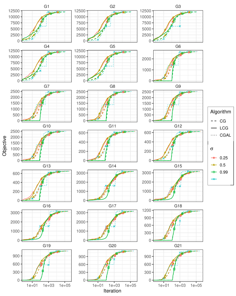
Figure 3: Max-Cut datasets G1-G21 objective function value vs. iteration.

Table 1: Max-Cut datasets

			$\operatorname{\texttt{SDPT3}}3$
Dataset	#Nodes	#Edges	Value	$\lambda_{\text{min}}$	Feas. value
G1	800	19176	12083.2	0	-
G2	800	19176	12089.43	0	-
G3	800	19176	12084.33	0	-
G4	800	19176	12111.5	0	-
G5	800	19176	12100	0	-
G6	800	19176	2667	0	-
G7	800	19176	2494.25	0	-
G8	800	19176	2535.25	0	-
G9	800	19176	12111.5	0	-
G10	800	19176	12111.5	0	-
G11	800	1600	634.83	0	-
G12	800	1600	628.41	0	-
G13	800	1600	651.54	0	-
G14	800	1600	12111.5	0	-
G15	800	4661	3171.56	0	-
G16	800	4672	3175.02	0	-
G17	800	4667	3171.25	0	-
G18	800	4694	1173.75	0	-
G19	800	4661	1091	0	-
G20	800	4672	1119	0	-
G21	800	4667	1112.06	0	-
G22	2000	19990	18276.89	-1	14135.95
G23	2000	19990	18289.22	-1	14142.11
G24	2000	19990	18286.75	-1	9997.75
G25	2000	19990	18293.5	-1	9996
G26	2000	19990	18270.24	-1	14132.87
G27	2000	19990	8304.5	-1	4141.75
G28	2000	19990	8253.5	-1	4100.75
G29	2000	19990	8377.75	-1	4209
G30	2000	19990	8381	-1	4215.5

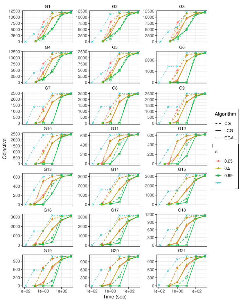
Figure 4: Max-Cut datasets G1-G21 objective function value vs. time.

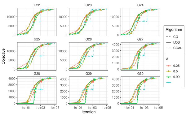
Figure 5: Max-Cut datasets G22-G30 objective function value vs. iteration.

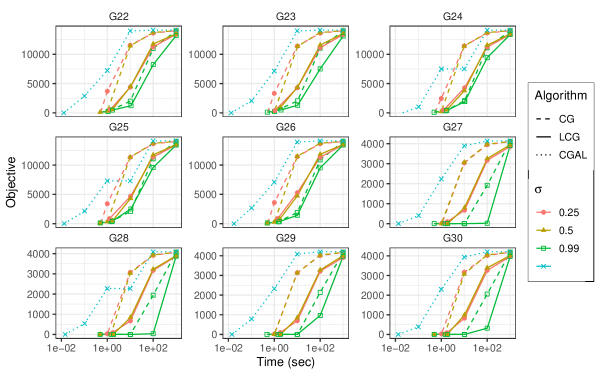
Figure 6: Max-Cut datasets G22-G30 objective function value vs. time.

Table 2: Performance for datasets G1-G30 after a certain number of iterations.

Data	Iter		Alg.	$\operatorname{\texttt{CG}}$			$\operatorname{\texttt{LCG}}$			$\operatorname{CGAL}$
			$\sigma$	0.25	0.5	0.99	0.25	0.5	0.99	-
		$g(z)$
		Gap
		Time
G1	100			7322	7023	6147	8998	9278	6781	6084
				39.40%	41.88%	49.13%	25.54%	23.21%	43.88%	49.65%
				0.9	1.5	15.1	7.2	7.5	21.4	0.2
	1000			11103	11099	10882	11158	11278	10945	11946
				8.11%	8.14%	9.95%	7.65%	6.66%	9.42%	1.13%
				4.8	5.7	41.7	62.8	63.5	101.9	2.7
	10000			11853	11864	11800	11801	11829	11760	12069
				1.91%	1.81%	2.34%	2.34%	2.11%	2.67%	0.12%
				46.3	50.2	103.7	586.4	598.3	657.5	38.8
	1e+05			12027	12030	12015	-	-	-	12082
				0.47%	0.44%	0.57%	-	-	-	0.01%
				761.1	774.6	782.5	-	-	-	635.3
G2	100			7196	7330	6197	8952	9223	6805	3363
				40.47%	39.37%	48.74%	25.95%	23.71%	43.71%	72.18%
				0.8	1.4	15.5	6.7	7.3	21.3	0.2
	1000			11099	11120	10885	11186	11283	10957	11930
				8.20%	8.01%	9.96%	7.47%	6.67%	9.37%	1.32%
				4.6	6.0	43.1	61.1	60.7	102.1	2.9
	10000			11860	11881	11810	11806	11838	11766	12075
				1.90%	1.73%	2.31%	2.35%	2.08%	2.68%	0.12%
				47.4	52.1	107.0	558.7	567.8	627.0	42.0
	1e+05			12030	12038	12019	-	-	-	12088
				0.49%	0.42%	0.58%	-	-	-	0.01%
				664.1	804.1	797.5	-	-	-	685.3
G3	100			7336	7258	6150	9227	8902	6654	6019
				39.30%	39.94%	49.11%	23.64%	26.34%	44.94%	50.19%
				0.8	1.4	15.4	7.7	8.2	21.6	0.2
	1000			11091	11109	10837	11250	11124	10894	6040
				8.22%	8.07%	10.32%	6.90%	7.94%	9.85%	50.02%
				4.8	5.3	43.6	62.3	71.2	98.4	2.6
	10000			11867	11882	11795	11844	11798	11767	12073
				1.80%	1.68%	2.39%	1.99%	2.37%	2.63%	0.09%
				47.1	50.0	111.9	578.5	595.3	639.2	39.2
	1e+05			12026	12036	12014	-	-	-	12083
				0.49%	0.40%	0.58%	-	-	-	0.01%
				773.1	806.3	855.6	-	-	-	646.1
G4	100			7180	6934	5995	8833	9156	6519	4137
				40.71%	42.75%	50.50%	27.07%	24.41%	46.18%	65.85%
				0.8	1.5	15.7	6.7	9.1	23.9	0.2
	1000			11329	11114	10885	11212	11286	10949	11969
				8.20%	8.23%	10.13%	7.43%	6.82%	9.60%	1.18%
				5.0	5.7	44.1	64.7	73.6	109.9	3.1
	10000			11904	11912	11834	11818	11866	11805	12082
				1.71%	1.65%	2.29%	2.43%	2.02%	2.53%	0.24%
				49.7	49.4	105.7	709.4	722.0	709.5	43.9
	1e+05			12051	12062	12043	-	-	-	12110
				0.50%	0.41%	0.56%	-	-	-	0.01%
				774.7	757.6	778.6	-	-	-	702.1
G5	100			7319	7360	6039	8910	9272	6713	4512
				39.51%	39.18%	50.09%	26.37%	23.37%	44.52%	62.71%
				0.8	1.6	15.4	6.8	8.6	23.4	0.2
	1000			11094	11137	10873	11128	11260	10926	11917
				8.31%	7.96%	10.14%	8.03%	6.95%	9.70%	1.51%
				4.8	5.8	43.0	63.3	73.3	108.7	3.0
	10000			11880	11898	11819	11815	11885	11784	12082
				1.81%	1.67%	2.32%	2.36%	1.78%	2.61%	0.15%
				47.4	53.5	106.5	700.9	686.1	708.3	42.6
	1e+05			12040	12053	12033	-	-	-	12099
				0.49%	0.38%	0.55%	-	-	-	0.01%
				766.0	845.9	847.6	-	-	-	691.3
G6	100			1305	1420	23	1721	1822	54	1317
				51.08%	46.75%	99.12%	35.47%	31.68%	97.96%	50.62%
				1.1	1.5	16.7	7.4	9.1	23.8	0.2
	1000			2272	2375	2388	2396	2446	2447	2602
				14.81%	10.95%	10.45%	10.16%	8.27%	8.24%	2.44%
				5.5	6.1	63.7	64.5	70.6	123.7	2.9
	10000			2579	2601	2604	2602	2613	2615	2653
				3.29%	2.46%	2.35%	2.43%	2.02%	1.96%	0.52%
				58.3	64.2	155.7	610.6	665.4	713.7	43.7
G7	100			1187	1349	446	1542	1727	531	1232
				52.39%	45.90%	82.11%	38.19%	30.74%	78.71%	50.61%
				1.0	1.4	15.7	7.0	10.3	25.0	0.2
	1000			2170	2239	2235	2221	2290	2285	2444
				13.01%	10.23%	10.37%	10.93%	8.18%	8.37%	2.00%
				5.1	6.2	59.2	74.8	80.8	134.5	3.1
	10000			2423	2438	2436	2431	2448	2443	2485
				2.86%	2.26%	2.32%	2.55%	1.87%	2.06%	0.37%
				56.3	69.1	143.8	744.4	785.4	807.1	44.0
G8	100			1258	1347	0	1658	1720	66	1245
				50.00%	46.46%	100.00%	34.10%	31.67%	97.36%	50.53%
				1.0	1.5	15.6	7.2	9.1	24.7	0.2
	1000			2197	2251	2252	2263	2307	2307	2439
				12.71%	10.55%	10.51%	10.09%	8.33%	8.31%	3.08%
				5.3	6.4	61.0	71.9	78.6	132.6	2.9
	10000			2442	2456	2458	2456	2467	2468	2501
				2.94%	2.39%	2.34%	2.40%	1.98%	1.93%	0.61%
				59.1	65.9	149.4	723.4	743.9	766.6	43.2
G9	100			1186	1304	342	1625	1694	40	1275
				53.21%	48.57%	86.52%	35.89%	33.20%	98.41%	49.71%
				1.1	1.5	15.5	7.7	8.4	23.8	0.2
	1000			2156	2255	2270	2273	2335	2326	2332
				14.96%	11.04%	10.45%	10.36%	7.89%	8.26%	8.00%
				5.0	6.1	63.3	68.0	71.6	126.5	2.8
	10000			2450	2473	2474	2473	2484	2483	2525
				3.37%	2.45%	2.40%	2.46%	2.01%	2.06%	0.42%
				53.4	62.6	158.0	654.3	680.7	738.8	41.6
G10	100			1218	1334	334	1586	1688	753	1245
				51.16%	46.53%	86.63%	36.42%	32.33%	69.79%	50.07%
				1.1	1.5	16.1	7.4	9.0	24.2	0.2
	1000			2128	2218	2229	2223	2294	2294	2441
				14.67%	11.08%	10.63%	10.88%	8.05%	8.02%	2.13%
				5.1	6.2	59.2	71.9	77.9	130.1	2.8
	10000			2420	2435	2436	2434	2446	2446	2480
				2.97%	2.40%	2.35%	2.40%	1.92%	1.95%	0.55%
				56.6	69.9	146.0	721.3	735.1	779.6	43.1
G11	100			318	349	113	438	449	206	308
				49.84%	45.00%	82.23%	30.93%	29.31%	67.56%	51.43%
				0.4	0.5	4.5	5.1	5.0	9.8	0.1
	1000			552	559	564	565	575	577	583
				13.09%	11.98%	11.22%	10.97%	9.44%	9.16%	8.11%
				2.3	2.8	17.0	44.1	43.4	61.3	1.1
	10000			611	611	613	614	613	614	628
				3.69%	3.70%	3.41%	3.32%	3.51%	3.22%	1.15%
				22.1	25.1	46.0	402.8	414.7	437.8	14.3
	1e+05			628	628	628	-	-	-	629
				1.04%	1.00%	1.00%	-	-	-	0.92%
				252.3	280.2	310.6	-	-	-	216.7
G12	100			301	335	122	424	431	156	296
				52.05%	46.70%	80.63%	32.55%	31.40%	75.24%	52.82%
				0.4	0.5	4.5	5.4	5.0	9.9	0.1
	1000			544	550	555	559	566	567	595
				13.45%	12.50%	11.67%	10.98%	9.93%	9.78%	5.30%
				2.7	2.7	16.9	47.6	44.3	61.3	1.2
	10000			605	604	607	607	606	607	622
				3.75%	3.84%	3.44%	3.38%	3.63%	3.34%	1.01%
				24.6	25.3	44.7	428.1	417.4	458.0	14.3
	1e+05			622	622	622	-	-	-	624
				1.01%	1.08%	1.02%	-	-	-	0.75%
				283.5	278.5	322.2	-	-	-	218.4
G13	100			318	357	132	446	450	215	317
				51.17%	45.15%	79.72%	31.61%	30.87%	67.03%	51.39%
				0.4	0.5	4.3	4.8	5.9	9.5	0.1
	1000			565	572	579	582	588	591	610
				13.25%	12.21%	11.09%	10.73%	9.71%	9.29%	6.34%
				2.4	2.4	16.6	41.5	54.8	66.0	1.2
	10000			626	628	630	629	629	631	645
				3.88%	3.68%	3.32%	3.38%	3.51%	3.21%	0.94%
				21.6	23.7	44.0	413.8	462.5	460.7	14.7
	1e+05			645	645	645	-	-	-	647
				1.06%	1.04%	0.97%	-	-	-	0.70%
				264.2	280.5	336.9	-	-	-	225.0
G14	100			1118	977	330	1311	1309	331	1482
				64.97%	69.39%	89.67%	58.91%	58.99%	89.64%	53.55%
				0.5	0.8	6.2	5.9	6.2	13.1	0.1
	1000			2219	2400	2461	2283	2490	2509	1529
				30.47%	24.79%	22.90%	28.48%	21.97%	21.40%	52.09%
				2.7	3.3	24.3	54.1	56.2	82.1	1.6
	10000			2952	2995	3045	2961	3021	3053	3185
				7.49%	6.16%	4.59%	7.22%	5.34%	4.33%	0.22%
				26.7	27.7	62.1	534.9	551.2	616.5	21.4
	1e+05			3144	3152	3161	-	-	-	3191
				1.49%	1.23%	0.96%	-	-	-	0.02%
				336.7	385.6	472.7	-	-	-	342.3
G15	100			1099	994	272	1272	1201	277	1428
				65.36%	68.65%	91.42%	59.90%	62.15%	91.26%	54.99%
				0.5	0.7	6.0	5.4	5.8	11.6	0.1
	1000			2147	2328	2390	2241	2444	2443	1541
				32.30%	26.61%	24.66%	29.34%	22.93%	22.98%	51.40%
				2.6	3.2	24.0	45.9	49.5	72.0	1.5
	10000			2920	2982	3015	2931	2988	3024	3166
				7.93%	5.99%	4.93%	7.60%	5.78%	4.65%	0.19%
				25.6	30.0	59.6	442.4	459.1	512.9	21.2
	1e+05			3118	3132	3140	-	-	-	3171
				1.70%	1.24%	1.00%	-	-	-	0.02%
				296.1	370.5	470.7	-	-	-	328.8
G16	100			1085	1014	369	1316	1284	371	1467
				65.83%	68.06%	88.37%	58.54%	59.56%	88.32%	53.78%
				0.5	0.6	6.1	5.2	5.3	11.3	0.1
	1000			2127	2379	2440	2322	2487	2491	1497
				33.02%	25.07%	23.15%	26.86%	21.68%	21.55%	52.85%
				3.1	3.0	23.0	45.5	46.9	68.3	1.3
	10000			2920	2996	3024	2946	3007	3031	3168
				8.03%	5.64%	4.76%	7.22%	5.30%	4.53%	0.21%
				26.7	27.6	60.6	439.5	450.8	484.9	18.0
	1e+05			3127	3137	3143	-	-	-	3175
				1.51%	1.19%	1.00%	-	-	-	0.01%
				324.0	375.2	477.0	-	-	-	296.5
G17	100			1095	1053	301	1383	1289	299	1481
				65.47%	66.80%	90.52%	56.41%	59.35%	90.56%	53.30%
				0.5	0.7	6.2	7.2	6.2	12.6	0.1
	1000			2163	2343	2402	2296	2435	2467	1517
				31.78%	26.13%	24.26%	27.61%	23.23%	22.21%	52.17%
				3.0	3.2	24.0	59.6	57.7	83.2	1.6
	10000			2897	2974	3015	2937	2994	3026	3166
				8.64%	6.22%	4.92%	7.40%	5.59%	4.58%	0.17%
				25.4	28.3	61.4	535.6	551.6	600.7	20.7
	1e+05			3120	3132	3139	-	-	-	3171
				1.60%	1.25%	1.02%	-	-	-	0.02%
				338.5	401.5	503.0	-	-	-	331.7
G18	100			531	546	0	680	710	0	562
				54.73%	53.50%	100.00%	42.08%	39.51%	100.00%	52.15%
				0.7	0.7	6.1	6.2	6.4	14.5	0.1
	1000			949	986	998	993	1012	1016	778
				19.19%	16.00%	14.97%	15.37%	13.78%	13.45%	33.74%
				3.5	3.7	26.1	54.8	56.0	88.9	1.5
	10000			1113	1131	1133	1128	1133	1141	1163
				5.21%	3.66%	3.49%	3.91%	3.46%	2.83%	0.94%
				36.0	39.3	74.6	540.7	545.3	615.7	19.3
	1e+05			1161	1164	1165	-	-	-	1166
				1.13%	0.84%	0.78%	-	-	-	0.69%
				457.7	568.7	719.1	-	-	-	314.3
G19	100			511	518	0	595	650	0	536
				53.17%	52.48%	100.00%	45.50%	40.42%	100.00%	50.87%
				0.6	0.8	6.3	6.6	7.2	13.8	0.1
	1000			895	925	923	907	937	952	538
				18.00%	15.27%	15.41%	16.86%	14.10%	12.79%	50.73%
				3.2	3.6	28.2	61.3	66.4	93.1	1.5
	10000			1034	1047	1055	1044	1053	1060	1079
				5.25%	4.05%	3.30%	4.35%	3.46%	2.81%	1.10%
				34.2	39.2	79.4	598.8	614.7	660.7	20.6
	1e+05			1079	1081	1083	-	-	-	1082
				1.09%	0.88%	0.77%	-	-	-	0.86%
				520.4	691.2	823.0	-	-	-	330.3
G20	100			507	526	0	670	661	0	542
				54.73%	53.02%	100.00%	40.08%	40.95%	100.00%	51.53%
				0.5	0.7	6.4	7.3	7.3	14.7	0.1
	1000			894	957	952	941	980	969	797
				20.14%	14.48%	14.95%	15.88%	12.45%	13.43%	28.73%
				3.1	3.9	26.5	66.8	63.1	89.2	1.6
	10000			1063	1080	1079	1075	1086	1086	1109
				4.97%	3.51%	3.53%	3.94%	2.95%	2.93%	0.92%
				34.7	43.2	72.4	625.4	631.6	670.4	21.9
	1e+05			1108	1110	1111	-	-	-	1111
				1.02%	0.82%	0.74%	-	-	-	0.69%
				516.1	629.0	744.3	-	-	-	334.5
G21	100			530	530	0	651	682	0	536
				52.30%	52.30%	100.00%	41.44%	38.70%	100.00%	51.82%
				0.6	0.7	5.9	5.8	5.9	12.3	0.1
	1000			902	950	951	929	974	963	1029
				18.92%	14.56%	14.48%	16.47%	12.44%	13.37%	7.51%
				3.3	3.7	25.7	51.9	50.8	75.3	1.2
	10000			1056	1072	1075	1067	1075	1081	1101
				5.04%	3.64%	3.35%	4.09%	3.36%	2.80%	0.99%
				34.2	43.2	71.0	490.7	474.6	521.7	17.7
	1e+05			1101	1103	1104	-	-	-	1104
				1.00%	0.81%	0.75%	-	-	-	0.73%
				506.1	672.2	695.8	-	-	-	289.9
G22	100			6625	6357	9384	9908	5184	6406	7177
				53.14%	55.03%	33.62%	29.91%	63.33%	54.68%	49.23%
				2.2	3.2	41.8	39.0	46.3	79.6	0.5
	1000			12305	12501	12747	13016	12404	12608	13096
				12.95%	11.56%	9.83%	7.92%	12.25%	10.81%	7.35%
				15.1	16.8	347.8	342.2	139.3	447.0	6.1
	10000			13737	13822	-	-	13776	-	14115
				2.82%	2.22%	-	-	2.55%	-	0.15%
				138.3	144.6	-	-	338.5	-	82.0
G23	100			6623	6456	9547	10036	5316	6560	7065
				53.17%	54.35%	32.49%	29.03%	62.41%	53.61%	50.04%
				2.4	3.4	47.7	44.4	50.8	88.8	0.5
	1000			12346	12547	12780	13105	12395	12631	13903
				12.70%	11.28%	9.63%	7.33%	12.36%	10.69%	1.69%
				16.6	18.3	409.3	401.3	139.2	518.5	6.4
	10000			13762	13838	-	-	13779	-	14121
				2.69%	2.15%	-	-	2.57%	-	0.15%
				152.2	158.4	-	-	350.0	-	79.8
G24	100			5664	6405	9347	9969	6938	9091	7212
				59.94%	54.70%	33.90%	29.50%	50.94%	35.71%	49.00%
				2.3	3.3	43.4	44.8	50.0	90.8	0.5
	1000			12305	12511	12868	13050	12606	12971	7067
				12.98%	11.53%	9.00%	7.71%	10.85%	8.27%	50.03%
				15.8	16.8	383.6	389.7	144.8	533.9	5.9
	10000			13746	13832	-	-	13816	-	14113
				2.79%	2.18%	-	-	2.29%	-	0.20%
				137.5	147.4	-	-	345.9	-	73.4
G25	100			6620	6428	9286	9868	6794	9025	7174
				53.20%	54.56%	34.35%	30.23%	51.97%	36.19%	49.28%
				2.9	3.2	38.5	39.8	49.8	84.3	0.5
	1000			12312	12518	12844	13027	12584	12963	7074
				12.95%	11.50%	9.19%	7.90%	11.03%	8.35%	49.99%
				16.1	17.3	344.9	346.4	144.1	483.6	6.1
	10000			13765	13838	-	-	13815	-	14121
				2.68%	2.17%	-	-	2.33%	-	0.16%
				143.5	147.5	-	-	341.8	-	75.2
G26	100			6634	6325	9381	9806	6610	8953	7075
				53.06%	55.24%	33.63%	30.61%	53.23%	36.65%	49.94%
				2.7	3.7	39.7	39.2	50.6	84.6	0.5
	1000			12294	12520	12859	13026	12554	12952	7066
				13.01%	11.41%	9.02%	7.83%	11.17%	8.35%	50.00%
				15.4	17.1	332.9	332.8	148.1	475.4	5.8
	10000			13746	13828	-	-	13798	-	14110
				2.74%	2.15%	-	-	2.37%	-	0.16%
				140.0	142.6	-	-	347.3	-	73.2
G27	100			1438	1761	2394	2572	0	0	2088
				65.27%	57.48%	42.20%	37.90%	100.00%	100.00%	49.58%
				3.9	4.8	40.6	39.9	49.1	92.2	0.5
	1000			3403	3538	3613	3759	3559	3734	2084
				17.83%	14.57%	12.76%	9.24%	14.08%	9.84%	49.68%
				17.3	19.0	344.8	343.6	182.0	522.7	5.8
	10000			3987	4030	-	-	4031	-	4132
				3.74%	2.71%	-	-	2.67%	-	0.24%
				149.7	161.2	-	-	394.9	-	73.1
G28	100			1426	1713	2382	2506	0	0	2075
				65.23%	58.23%	41.90%	38.90%	100.00%	100.00%	49.40%
				3.4	4.9	36.3	37.1	49.2	93.4	0.5
	1000			3376	3511	3581	3697	3534	3695	2045
				17.68%	14.37%	12.68%	9.85%	13.81%	9.89%	50.13%
				16.6	19.7	313.1	338.7	182.1	533.1	6.0
	10000			3951	3990	-	-	3990	-	4090
				3.64%	2.70%	-	-	2.71%	-	0.27%
				146.6	160.0	-	-	394.7	-	72.8
G29	100			1432	1765	2366	2536	62	254	2117
				65.97%	58.06%	43.78%	39.75%	98.52%	93.97%	49.69%
				3.4	4.3	39.9	39.7	47.2	89.8	0.5
	1000			3452	3580	3659	3768	3614	3798	2104
				17.97%	14.93%	13.07%	10.47%	14.14%	9.77%	50.01%
				17.2	19.2	338.4	351.4	177.8	522.0	5.5
	10000			4047	4071	-	-	4091	-	4196
				3.84%	3.27%	-	-	2.80%	-	0.30%
				150.1	163.8	-	-	391.3	-	71.3
G30	100			1467	1753	2426	2665	19	68	2108
				65.21%	58.42%	42.45%	36.77%	99.55%	98.40%	49.99%
				3.4	4.7	37.0	38.3	48.6	94.9	0.5
	1000			3453	3591	3670	3842	3622	3783	2110
				18.09%	14.81%	12.93%	8.86%	14.09%	10.26%	49.95%
				16.4	19.2	323.7	334.9	180.1	537.4	6.1
	10000			4059	4082	-	-	4101	-	4205
				3.71%	3.18%	-	-	2.72%	-	0.24%
				149.6	162.4	-	-	398.4	-	73.4

B.2 Markov chain mixing rate

We next consider the problem of finding the fastest mixing rate of a Markov chain on a graph [31]. In this problem, a symmetric Markov chain is defined on an undirected graph $G=(\{1,\ldots,n\},\mathcal{E})$. Given $G$ and weights $d_{ij}$ for $\{i,j\}\in\mathcal{E}$, we are tasked with finding the transition rates $w_{ij}\geq 0$ for each $\{i,j\}\in\mathcal{E}$ with weighted sum smaller than 1, that result in the fastest mixing rate. We assume that $\sum_{ij}d^{2}_{ij}=n^{2}$. The mixing rate is given by the second smallest eigenvalue of the graph’s Laplacian matrix, described as

$$L(\mathbf{w})_{ij}=\begin{cases}\sum_{j:\{i,j\}\in\mathcal{E}}w_{ij}&j=i\\ -w_{ij}&\{i,j\}\in\mathcal{E}\\ 0&\text{otherwise}.\end{cases}.$$

From $L\mathbf{1}=0$ it follows that $\frac{1}{n}\mathbf{1}$ is a stationary distribution of the process. From [7], we have the following bound on the total variation distance of the time $t$ distribution of the Markov process and the stationary distribution $\sup_{\pi}\lVert\pi{\mathbf{P}}(t)-\frac{1}{n}\mathbf{1}\rVert_{\text{TV}}\leq\frac{1}{2}\sqrt{n}e^{-\lambda t}.$ The quantity $T_{\text{mix}}=\lambda$ is called the mixing time, and $\lambda\equiv\lambda_{2}(L(\mathbf{w}))$ is the second-largest eigenvalue of the graph Laplacian $L(\mathbf{w})$. To bound this eigenvalue, we follow the strategy laid out in [31]. Thus, the problem can be written as

$$\max_{\mathbf{w}}\quad \lambda_{2}(L(\mathbf{w}))$$

s.t. $$\sum_{\{i,j\}\in\mathcal{E}}d_{ij}^{2}w_{ij}\leq 1$$

$$\mathbf{w}\geq 0.$$

This problem can also alternatively be formulated as

$$\min_{\mathbf{w}}\quad \sum_{\{i,j\}\in\mathcal{E}}d_{ij}^{2}w_{ij}$$

s.t. $$\lambda_{2}(L(\mathbf{w}))\geq 1$$

$$\mathbf{w}\geq 0.$$

Due to the properties of the Laplacian, the first constraint can be reformulated as

$$\min_{\mathbf{w}}\quad \sum_{\{i,j\}\in\mathcal{E}}d_{ij}^{2}w_{ij}$$ (B.2)

s.t. $$L(\mathbf{w})\succeq\mathbf{I}_{n\times n}-\frac{1}{n}\mathbf{1}\mathbf{1}^{\top}$$ (B.3)

$$\mathbf{w}\geq 0.$$ (B.4)

The dual problem is then given by

$$\begin{split}\max_{\mathbf{X}\in\mathbb{S}^{n}_{+}}\quad&\langle\mathbf{I}_{n\times n}-\frac{1}{n}\mathbf{1}\mathbf{1}^{\top},\mathbf{X}\rangle\\ \text{s.t.}\quad&X_{ii}+X_{jj}-2X_{ij}\leq d_{ij}^{2}\qquad\{i,j\}\in\mathcal{E}\end{split}$$ (B.5)

To obtain an SDP within our convex programming model, we combine arguments from [31] and [1]. Let $\mathbf{X}$ be a feasible point for (B.5). Then, there exists a $n\times n$ matrix ${\mathbf{V}}$ such that $\mathbf{X}={\mathbf{V}}{\mathbf{V}}^{\top}$. It is easy to see that multiplying each row of the matrix ${\mathbf{V}}^{\top}=[\mathbf{v}_{1},\ldots,\mathbf{v}_{n}]$ with an orthonormal matrix does not change the feasibility of the candidate solution. Moreover $X_{ij}=\mathbf{v}_{i}^{\top}\mathbf{v}_{j}$ for all $1\leq i,j\leq n$, so that $X_{ii}+X_{jj}-2X_{ij}=\lVert\mathbf{v}_{i}-\mathbf{v}_{j}\rVert^{2}_{2}$. Since shifting each vector $\mathbf{v}_{i}$ by a constant vector $\mathbf{v}$ would not affect the objective or constraints, we can, without loss of generality, set $\mathbf{v}_{1}=\mathbf{0}$. This gives the equivalent optimization problem

$$\begin{split}\max_{\mathbf{v}_{1},\ldots,\mathbf{v}_{n}}\quad&\sum_{i=1}^{n}\lVert\mathbf{v}_{i}\rVert^{2}\\ \text{s.t.}\quad&\lVert\mathbf{v}_{i}-\mathbf{v}_{j}\rVert^{2}\leq d^{2}_{ij}\qquad\{i,j\}\in\mathcal{E},\\ &\mathbf{v}_{i}\in\mathbb{R}^{n},\mathbf{v}_{1}=\mathbf{0}.\end{split}$$ (B.6)

This is the geometric dual derived in [31], which is strongly connected to the geometric embedding of a graph in the plane [18]. Thus, setting again $\mathbf{X}={\mathbf{V}}{\mathbf{V}}^{\top}$, we therefore obtain that $X_{1j}=X_{j1}=0$ for all $i=1,\ldots,n$ thus reducing the dimension of the problem, and (B.7) can be reformulated as follows:

$$\begin{split}\max_{\mathbf{X}\in\mathbb{S}^{n-1}_{+}}\quad&\langle\mathbf{I}_{{n-1}\times{n-1}}-\frac{1}{n}\mathbf{1}\mathbf{1}^{\top},\mathbf{X}\rangle\\ \text{s.t.}\quad&X_{(i-1)(i-1)}+X_{(j-1)(j-1)}-2X_{(i-1)(j-1)}\leq d_{ij}^{2}\qquad\{i,j\}\in\mathcal{E},i,j>1\\ &X_{(j-1)(j-1)}\leq d_{1j}^{2}\qquad\qquad\qquad\qquad\qquad\qquad\{1,j\}\in\mathcal{E}\end{split}$$ (B.7)

Moreover, since $\mathbf{X}\in\mathbb{S}^{n-1}_{+}$, it follows that $2|X_{ij}|\geq-\sqrt{X_{ii}X_{jj}}$ and so for any $\{i,j\}\in\mathcal{E}$ such that $i,j>1$ $\sqrt{X_{(j-1)(j-1)}}\leq\sqrt{X_{(i-1)(i-1)}}+\sqrt{d_{ij}}$. Therefore, since the graph is connected, we can recursively bound each diagonal element of $\mathbf{X}$ and therefore the trace by a constant $\alpha$, and add the trace constraint $\mathsf{X}=\{\mathbf{X}\in\mathbb{S}^{n}|\mathbf{X}\succeq 0,\operatorname{tr}(\mathbf{X})\leq\alpha\}$ to the problem formulation without affecting the optimal values. Moreover, defining $\mathcal{D}:\mathbb{S}^{n-1}\to\mathbb{R}^{\lvert\mathcal{E}\rvert}$ by

$$\mathcal{D}(\mathbf{X})_{\{i,j\}}=\begin{cases}X_{(i-1)(i-1)}+X_{(j-1)(j-1)}-2X_{(i-1)(j-1)},&i,j>0,\\ X_{(j-1)(j-1)},&i=1.\end{cases}$$

Let $\mathsf{Q}=\{\mathbf{y}\in\mathbb{R}^{\lvert\mathcal{E}\rvert}|y_{i,j}\leq d^{2}_{ij},\{i,j\}\in\mathcal{E}\}$ and $\mathsf{K}=\{(y,t)\in\mathbb{R}^{\lvert\mathcal{E}\rvert}\times\mathbb{R}|\frac{1}{t}y\in\mathsf{Q},t>0\}$. This is a closed convex cone with logarithmically homogeneous barrier

$$f(y,t)=-\sum_{\{i,j\}\in\mathcal{E}}\log(td^{2}_{ij}-y_{i,j})=-\sum_{e\in\mathcal{E}}\log(d^{2}_{ij}-\frac{1}{t}y_{i,j})-\lvert\mathcal{E}\rvert\log(t).$$

This gives a logarithmically homogeneous barrier $F(\mathbf{X},t)=f(\mathcal{P}(\mathbf{X},t))$, where $\mathcal{P}(\mathbf{X},t)=[\mathcal{D}(\mathbf{X});t]\in\mathbb{R}^{\lvert\mathcal{E}\rvert}\times\mathbb{R}$. We thus arrive at a formulation of the form of problem (P), which reads explicitly as

$$\begin{split}\min_{\mathbf{X}\in\mathbb{S}^{n}_{+},t>0}\quad&\langle\mathbf{I}_{n\times n}-\frac{1}{n}\mathbf{1}\mathbf{1}^{\top},\mathbf{X}\rangle\\ \text{s.t.}\quad&\mathcal{P}(\mathbf{X},t)\in\mathsf{K},t=1\\ &\mathbf{X}\in\mathsf{X}.\end{split}$$ (B.8)

Dataset	# Nodes	# Edges	SDPT3 Value
1	100	1000	15.62
2	100	2000	7.93
3	200	1000	72.32
4	200	4000	17.84
5	400	1000	388.52
6	400	8000	38.37
7	800	4000	333.25
8	800	16000	80.03

Table 3: Mixing datasets characteristics.

We generated random connected undirected graphs of various sizes, and for each edge $\{i,j\}$ in the graph we generated a random $d_{ij}^{2}$ uniformly in $[0,1]$. Table 3 provides the size of each dataset, and the value obtained by solving the Mixing problem SDP using CVX with the SDPT3 solver. In order to compare to the $\operatorname{CGAL}$ algorithm, we used the normalization guidelines specified in [39], so that the norm of the coefficients vector of each constraint will be equal to each other, and the norm of the constraint matrix and the objective matrix equals 1.

All datasets were run for both $\operatorname{\texttt{CG}}$ and $\operatorname{\texttt{LCG}}$ options with the following choice of parameters $\eta_{0}\in\{0.5\Omega_{g},1\Omega_{g},2\Omega_{g}\}$ and $\sigma\in\{0.9,0.5,0.25\}$. Since $\operatorname{CGAL}$ does not generate feasible solutions, we computed the deviation from feasibility of its outputed solution $\mathbf{X}^{\operatorname{CGAL}}$ by

$$\text{Relative Feasibility Gap}=\gamma(\mathbf{X}^{\operatorname{CGAL}})\equiv\max_{\{i,j\}\in\mathcal{E}}\frac{d_{ij}^{2}-\mathcal{D}(\mathbf{X}^{\operatorname{CGAL}})_{ij}}{d_{ij}^{2}}.$$

We then corrected the solution to a feasible solution $\tilde{\mathbf{X}}^{\operatorname{CGAL}}=\mathbf{X}^{\operatorname{CGAL}}/(\gamma(\mathbf{X}^{\operatorname{CGAL}})+1)$, however in our numerical experiments it turned out that $\gamma$ was extremely large, which resulted in $\tilde{\mathbf{X}}^{\operatorname{CGAL}}$ being very close to the zero matrix with very poor performance. Therefore, we used the following alternative iterative correction method: We set $\hat{\mathbf{X}}^{\operatorname{CGAL},1}=\mathbf{X}^{\operatorname{CGAL}}$, and at each iteration $k$ we identify $\{i,j\}\in\mathcal{E}$ which leads to the maximum value for $\gamma(\hat{\mathbf{X}}^{\operatorname{CGAL},k})$ set $i^{*}=\operatorname*{argmax}_{l\in\{i,j\}}X_{l}l$ and set

$$\hat{\mathbf{X}}^{\operatorname{CGAL},k+1}_{ij}=\begin{cases}\hat{\mathbf{X}}^{\operatorname{CGAL},k+1}_{ij},&i,j\neq i^{*}.\\ \hat{\mathbf{X}}^{\operatorname{CGAL},k+1}_{ij}/(\gamma(\hat{\mathbf{X}}^{\operatorname{CGAL},k})+1),&i=i^{*}\text{ or }j=i^{*}.\end{cases}.$$

We terminate the algorithm when $\gamma(\hat{(}\mathbf{X})^{\operatorname{CGAL},k})=0$. The value of the outputted $\hat{\mathbf{X}}^{\operatorname{CGAL}}$ is then computed.

We stopped each run after it reached at $10000$ iterations, or $3600$ seconds running time. Figures 7-8 illustrate the results for some of the parameter values. Table LABEL:tbl:MixingDataSetsResults displays the numerical values obtained from our experiments with the best configuration of parameters $\eta_{0}$ and $\sigma$.

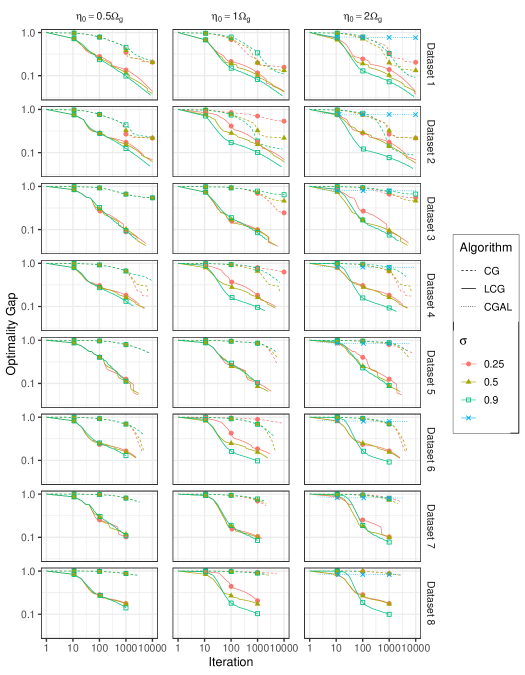
Figure 7: Mixing datasets relative gap from SDPT3 solution vs. iteration for various parameter choices.

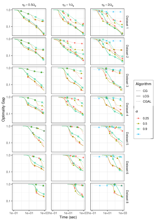
Figure 8: Mixing datasets relative gap from SDPT3 solution vs. time for various parameter choices.

Table 4: Mixing datasets results. For each dataset, time, and algorithm provides the best parameter choice for $\eta_{0}$ and $\sigma$, the function value obtained, the relative gap from the SDPT3 solution, the iteration, and the feasibility gap of the most recent solution.

Dataset	Time	Alg.	$\eta_{0}$ ($x\cdot\Omega_{g}$)	$\sigma$	Obj. Value	Rel. Gap	Iter.	Feas. Gap
1	100	CG	2	0.5	13.03	16.6%	2385	-
		LCG	2	0.9	14.39	7.9%	809	-
		CGAL	-	-	3.68	76.4%	3090	21930.2%
	500	CG	2	0.9	13.96	10.7%	4969	-
		LCG	2	0.25	14.97	4.1%	9001	-
		CGAL	-	-	3.74	76.1%	11460	12304.4%
	1000	CG	2	0.9	14.20	9.1%	9286	-
		LCG	0.5	0.25	15.12	3.2%	13598	-
		CGAL	-	-	3.76	75.9%	19981	8873.5%
2	100	CG	2	0.9	6.71	15.3%	957	-
		LCG	2	0.9	7.26	8.4%	745	-
		CGAL	-	-	1.88	76.2%	2948	19184.7%
	500	CG	2	0.9	7.17	9.5%	4099	-
		LCG	2	0.9	7.49	5.5%	3873	-
		CGAL	-	-	1.90	76.0%	10864	8729.7%
	1000	CG	2	0.9	7.23	8.8%	8024	-
		LCG	2	0.9	7.59	4.3%	7758	-
		CGAL	-	-	1.91	76.0%	18977	6066.0%
3	100	CG	1	0.25	32.86	54.6%	1865	-
		LCG	0.5	0.25	65.70	9.2%	888	-
		CGAL	-	-	15.15	79.1%	1656	44622.3%
	500	CG	1	0.25	54.34	24.9%	8832	-
		LCG	1	0.25	68.88	4.8%	3289	-
		CGAL	-	-	15.30	78.8%	6080	13031.6%
	1000	CG	1	0.25	54.87	24.1%	14128	-
		LCG	1	0.25	69.34	4.1%	5851	-
		CGAL	-	-	15.32	78.8%	10657	7902.7%
4	100	CG	2	0.25	10.28	42.4%	1676	-
		LCG	2	0.9	15.42	13.6%	166	-
		CGAL	-	-	3.33	81.3%	1440	116332.0%
	500	CG	0.5	0.25	14.69	17.7%	4710	-
		LCG	2	0.9	16.15	9.5%	921	-
		CGAL	-	-	3.36	81.2%	5203	57781.9%
	1000	CG	0.5	0.25	14.72	17.5%	6939	-
		LCG	2	0.9	16.47	7.7%	1880	-
		CGAL	-	-	3.36	81.2%	9081	41696.7%
5	100	CG	2	0.25	92.61	76.2%	1289	-
		LCG	1	0.25	340.02	12.5%	415	-
		CGAL	-	-	59.39	84.7%	946	122971.0%
	500	CG	0.5	0.9	163.46	57.9%	4788	-
		LCG	0.5	0.5	360.70	7.2%	1701	-
		CGAL	-	-	59.31	84.7%	3397	126861.0%
	1000	CG	1	0.25	277.79	28.5%	5359	-
		LCG	2	0.25	367.26	5.5%	2937	-
		CGAL	-	-	59.90	84.6%	5939	64948.0%
6	100	CG	1	0.5	10.52	72.6%	751	-
		LCG	2	0.25	30.11	21.5%	256	-
		CGAL	-	-	7.44	80.6%	811	149166.0%
	500	CG	0.5	0.25	28.98	24.5%	2995	-
		LCG	2	0.9	33.59	12.5%	232	-
		CGAL	-	-	7.60	80.2%	3004	103077.0%
	1000	CG	0.5	0.25	32.30	15.8%	4661	-
		LCG	2	0.9	34.24	10.8%	482	-
		CGAL	-	-	7.66	80.0%	5270	68409.9%
7	100	CG	0.5	0.9	35.69	89.3%	496	-
		LCG	1	0.25	276.90	16.9%	82	-
		CGAL	-	-	59.19	82.2%	478	702281.0%
	500	CG	1	0.25	102.57	69.2%	984	-
		LCG	0.5	0.25	295.47	11.3%	616	-
		CGAL	-	-	62.41	81.3%	1766	239810.0%
	1000	CG	1	0.25	152.56	54.2%	2101	-
		LCG	1	0.25	301.48	9.5%	1447	-
		CGAL	-	-	62.78	81.2%	3124	185699.0%
8	100	CG	0.5	0.9	4.49	94.4%	306	-
		LCG	0.5	0.25	55.80	30.3%	66	-
		CGAL	-	-	13.77	82.8%	431	613444.0%
	500	CG	0.5	0.9	12.03	85.0%	1455	-
		LCG	2	0.25	63.64	20.5%	566	-
		CGAL	-	-	13.99	82.5%	1593	282965.0%
	1000	CG	0.5	0.9	15.84	80.2%	2751	-
		LCG	1	0.9	66.98	16.3%	133	-
		CGAL	-	-	14.05	82.4%	2817	243686.0%

In the experiments we observe that the line search version $\operatorname{\texttt{LCG}}$ outperforms $\operatorname{\texttt{CG}}$ by orders of magnitude, although each iteration takes longer. One explanation of this is that the step size policy employed in $\operatorname{\texttt{CG}}$ is based on global optimization ideas which do not take into account the local structure of the problem. Line search captures these local features of the problem much better, leading to better numerical performance. Comparatively, $\operatorname{CGAL}$ performance is very poor, with optimality gaps around $70\%-90\%$, one conjecture for these results is that $\operatorname{CGAL}$ convergence guarantees depend on the magnitude of the dual variables, which in turn depend on the size of the Slater condition gap. Since the right-hand-side of the constraints, $d_{ij}^{2}$ may be very small, this gap will generally be small, and so the norm of the dual variables may be large, leading to a slow convergence. This also explain the difference with the superior performance $\operatorname{CGAL}$ exhibits in the Max-Cut example.

References

• Arora et al. [2005] S. Arora, E. Hazan, and S. Kale. Fast algorithms for approximate semidefinite programming using the multiplicative weights update method. In 46th Annual IEEE Symposium on Foundations of Computer Science (FOCS’05), pages 339–348, 2005. doi: 10.1109/SFCS.2005.35.
• Bandeira et al. [2016] Afonso S. Bandeira, Nicolas Boumal, and Vladislav Voroninski. On the low-rank approach for semidefinite programs arising in synchronization and community detection. In Vitaly Feldman, Alexander Rakhlin, and Ohad Shamir, editors, 29th Annual Conference on Learning Theory, volume 49 of Proceedings of Machine Learning Research, pages 361–382, Columbia University, New York, New York, USA, 23–26 Jun 2016. PMLR. URL https://proceedings.mlr.press/v49/bandeira16.html.
• Boyd and Vandenberghe [2004] Stephen Boyd and Lieven Vandenberghe. Convex optimization. Cambridge university press, 2004. ISBN 1107394007.
• Charikar and Wirth [2004] M. Charikar and A. Wirth. Maximizing quadratic programs: extending grothendieck’s inequality. In 45th Annual IEEE Symposium on Foundations of Computer Science, pages 54–60, 2004. doi: 10.1109/FOCS.2004.39.
• CVX Research [2012] Inc. CVX Research. CVX: Matlab software for disciplined convex programming, version 2.0. http://cvxr.com/cvx, August 2012.
• d’Aspremont et al. [2008] Alexandre d’Aspremont, Francis Bach, and Laurent El Ghaoui. Optimal solutions for sparse principal component analysis. Journal of Machine Learning Research, 9(7), 2008.
• Diaconis and Stroock [1991] Persi Diaconis and Daniel W. Stroock. Geometric bounds for eigenvalues of Markov chains. Annals of Applied Probability, 1:36–61, 1991.
• Dunn and Harshbarger [1978] J. C Dunn and S Harshbarger. Conditional gradient algorithms with open loop step size rules. Journal of Mathematical Analysis and Applications, 62(2):432–444, 1978. doi: https://doi.org/10.1016/0022-247X(78)90137-3. URL https://www.sciencedirect.com/science/article/pii/0022247X78901373.
• Dvurechensky et al. [2020] Pavel Dvurechensky, Petr Ostroukhov, Kamil Safin, Shimrit Shtern, and Mathias Staudigl. Self-concordant analysis of Frank-Wolfe algorithms. In Hal Daume III and Aarti Singh, editors, Proceedings of the 37th International Conference on Machine Learning, volume 119 of Proceedings of Machine Learning Research, pages 2814–2824, Virtual, 13–18 Jul 2020. PMLR. URL http://proceedings.mlr.press/v119/dvurechensky20a.html. arXiv:2002.04320.
• Dvurechensky et al. [2021] Pavel Dvurechensky, Shimrit Shtern, and Mathias Staudigl. First-order methods for convex optimization. EURO Journal on Computational Optimization, 9:100015, 2021. ISSN 2192-4406. doi: https://doi.org/10.1016/j.ejco.2021.100015. URL https://www.sciencedirect.com/science/article/pii/S2192440621001428. arXiv:2101.00935.
• Dvurechensky et al. [2022] Pavel Dvurechensky, Kamil Safin, Shimrit Shtern, and Mathias Staudigl. Generalized self-concordant analysis of frank–wolfe algorithms. Mathematical Programming, 2022. doi: 10.1007/s10107-022-01771-1. URL https://doi.org/10.1007/s10107-022-01771-1.
• Elbassioni et al. [2022] Khaled Elbassioni, Kazuhisa Makino, and Waleed Najy. Finding sparse solutions for packing and covering semidefinite programs. SIAM Journal on Optimization, 32(2):321–353, 2022. doi: 10.1137/20M137570X. URL https://doi.org/10.1137/20M137570X.
• Fawzi et al. [2019] Hamza Fawzi, James Saunderson, and Pablo A Parrilo. Semidefinite approximations of the matrix logarithm. Foundations of Computational Mathematics, 19:259–296, 2019.
• Faybusovich and Zhou [2020] Leonid Faybusovich and Cunlu Zhou. Self-concordance and matrix monotonicity with applications to quantum entanglement problems. Applied Mathematics and Computation, 375:125071, 2020. doi: https://doi.org/10.1016/j.amc.2020.125071. URL https://www.sciencedirect.com/science/article/pii/S0096300320300400.
• Frank and Wolfe [1956] Marguerite Frank and Philip Wolfe. An algorithm for quadratic programming. Naval Research Logistics Quarterly, 3(1-2):95–110, 2019/09/05 1956. doi: 10.1002/nav.3800030109. URL https://doi.org/10.1002/nav.3800030109.
• Freund and Grigas [2016] Robert M Freund and Paul Grigas. New analysis and results for the frank–wolfe method. Mathematical Programming, 155(1-2):199–230, 2016.
• Goemans and Williamson [1995] Michel X Goemans and David P Williamson. Improved approximation algorithms for maximum cut and satisfiability problems using semidefinite programming. Journal of the ACM (JACM), 42(6):1115–1145, 1995.
• Göring et al. [2008] Frank Göring, Christoph Helmberg, and Markus Wappler. Embedded in the shadow of the separator. SIAM Journal on Optimization, 19(1):472–501, 2008. doi: 10.1137/050639430. URL https://doi.org/10.1137/050639430.
• Hale et al. [2008] Elaine T. Hale, Wotao Yin, and Yin Zhang. Fixed-point continuation for $\ell_{1}$-minimization: Methodology and convergence. SIAM Journal on Optimization, 19(3):1107–1130, 2008. doi: 10.1137/070698920. URL https://doi.org/10.1137/070698920.
• Horodecki et al. [1996] Michał Horodecki, Paweł Horodecki, and Ryszard Horodecki. Separability of mixed states: necessary and sufficient conditions. Physics Letters A, 223(1):1–8, 1996. doi: https://doi.org/10.1016/S0375-9601(96)00706-2. URL https://www.sciencedirect.com/science/article/pii/S0375960196007062.
• Iyengar et al. [2011] G. Iyengar, D. J. Phillips, and C. Stein. Approximating semidefinite packing programs. SIAM Journal on Optimization, 21(1):231–268, 2011. doi: 10.1137/090762671. URL https://doi.org/10.1137/090762671.
• Iyengar et al. [2010] Garud Iyengar, David J Phillips, and Cliff Stein. Feasible and accurate algorithms for covering semidefinite programs. Scandinavian Workshop on Algorithm Theory, pages 150–162, 2010.
• Jaggi [2013] Martin Jaggi. Revisiting Frank-Wolfe: Projection-free sparse convex optimization. In International Conference on Machine Learning, pages 427–435, 2013.
• Lacoste-Julien et al. [2013] Simon Lacoste-Julien, Martin Jaggi, Mark Schmidt, and Patrick Pletscher. Block-coordinate Frank-Wolfe optimization for structural SVMs. In Sanjoy Dasgupta and David McAllester, editors, Proceedings of the 30th International Conference on Machine Learning, volume 28 of Proceedings of Machine Learning Research, pages 53–61, Atlanta, Georgia, USA, 2013. PMLR. URL https://proceedings.mlr.press/v28/lacoste-julien13.html.
• Lanckriet et al. [2004] Gert RG Lanckriet, Nello Cristianini, Peter Bartlett, Laurent El Ghaoui, and Michael I Jordan. Learning the kernel matrix with semidefinite programming. Journal of Machine learning research, 5(Jan):27–72, 2004.
• Laurent and Rendl [2005] Monique Laurent and Franz Rendl. Semidefinite programming and integer programming. Handbooks in Operations Research and Management Science, 12:393–514, 2005.
• Nesterov [2018] Yurii Nesterov. Lectures on Convex Optimization, volume 137 of Springer Optimization and Its Applications. Springer International Publishing, 2018.
• Nesterov and Nemirovski [1994] Yurii Nesterov and Arkadi Nemirovski. Interior Point Polynomial methods in Convex programming. SIAM Publications, 1994.
• Nielsen and Chuang [2010] M. Nielsen and I Chuang. Quantum Computation and Quantum Information. Cambridge: Cambridge University Press., 2010.
• Peng and Wei [2007] Jiming Peng and Yu Wei. Approximating k-means-type clustering via semidefinite programming. SIAM Journal on Optimization, 18(1):186–205, 2007. doi: 10.1137/050641983. URL https://doi.org/10.1137/050641983.
• Sun et al. [2006] Jun Sun, Stephen Boyd, Lin Xiao, and Persi Diaconis. The fastest mixing markov process on a graph and a connection to a maximum variance unfolding problem. SIAM Review, 48(4):681–699, 2022/01/12/ 2006. URL http://www.jstor.org/stable/20453871.
• Tibshirani and Taylor [2011] Ryan J. Tibshirani and Jonathan Taylor. The solution path of the generalized lasso. Ann. Statist., 39(3):1335–1371, 2011. doi: 10.1214/11-AOS878. URL https://projecteuclid.org:443/euclid.aos/1304514656.
• Weinberger and Saul [2009] Kilian Q Weinberger and Lawrence K Saul. Distance metric learning for large margin nearest neighbor classification. Journal of machine learning research, 10(2), 2009.
• Wen et al. [2010] Zaiwen Wen, Wotao Yin, Donald Goldfarb, and Yin Zhang. A fast algorithm for sparse reconstruction based on shrinkage, subspace optimization, and continuation. SIAM Journal on Scientific Computing, 32(4):1832–1857, 2010. doi: 10.1137/090747695. URL https://doi.org/10.1137/090747695.
• Xiao and Zhang [2013] Lin Xiao and Tong Zhang. A proximal-gradient homotopy method for the sparse least-squares problem. SIAM Journal on Optimization, 23(2):1062–1091, 2013. doi: 10.1137/120869997. URL https://doi.org/10.1137/120869997.
• [36] Yinyu Ye. GSet random graphs dataset. http://web.stanford.edu/~yyye/yyye/Gset/. Accessed July, 2022.
• [37] Alp Yurtsever. SketchyCGAL MATLAB code. URL https://github.com/alpyurtsever/SketchyCGAL.
• Yurtsever et al. [2018] Alp Yurtsever, Olivier Fercoq, Francesco Locatello, and Volkan Cevher. A conditional gradient framework for composite convex minimization with applications to semidefinite programming. pages 5727–5736. PMLR, 2018. ISBN 2640-3498.
• Yurtsever et al. [2021] Alp Yurtsever, Joel A. Tropp, Olivier Fercoq, Madeleine Udell, and Volkan Cevher. Scalable semidefinite programming. SIAM Journal on Mathematics of Data Science, 3(1):171–200, 2021. doi: 10.1137/19M1305045. URL https://doi.org/10.1137/19M1305045.
• Zhao [2023] Renbo Zhao. An away-step frank-wolfe method for minimizing logarithmically-homogeneous barriers. arXiv preprint arXiv:2305.17808, 2023.
• Zhao and Freund [2022] Renbo Zhao and Robert M. Freund. Analysis of the Frank–Wolfe method for convex composite optimization involving a logarithmically-homogeneous barrier. Mathematical Programming, 2022. doi: 10.1007/s10107-022-01820-9. URL https://doi.org/10.1007/s10107-022-01820-9.
• Zinchenko et al. [2010] Yuriy Zinchenko, Shmuel Friedland, and Gilad Gour. Numerical estimation of the relative entropy of entanglement. Physical Review A, 82(5):052336, 2010.