Maximum of Branching Brownian Motion among mild obstacles

Abstract.

We study the height of the maximal particle at time $t$ of a one dimensional branching Brownian motion with a space-dependent branching rate. The branching rate is set to zero in finitely many intervals (obstacles) of order $t$. We obtain almost sure asymptotics of the first order of the maximum, describe the path of a particle reaching this height and describe its dependence on the size and location of the obstacles.

1. Introduction

Standard branching Brownian motion is a prototype for a spatial branching process, which has been studied extensively in the last decades also due to its connection with the F-KPP equation [21, 28, 24, 25, 26]. It was shown by Bramson [12, 13] that the position of the maximal particle at time $t$ is tight around

$$m(t)=\sqrt{2}t-\frac{3}{2\sqrt{2}}\log(t)$$ (1.1)

and the convergence of the extremal process was proven in [3, 1]. There are several ways to introduce inhomogeneities into branching Brownian motion. Branching Brownian motion with time inhomogeneous variance has been studied extensively in [19, 8, 9, 20, 30, 10]. Certain instances of branching Brownian motion with space inhomogeneous branching rate have been analysed in [7, 33], where the branching rate is a function of the distance to the origin. Moreover, branching Brownian motion with (mild) obstacles has been studied in [17, 31, 18] focusing mainly on the total population size. In the present article, we consider a one dimensional branching Brownian motion for time $t$, in which the branching is suppressed in space intervals of order $t$.

1.1. The model

In this article, we study a one dimensional branching Brownian motion (BBM) with space inhomogeneous branching rate. More precisely, we consider a BBM for a time horizon $t$, that does not branch in some space intervals of order $t$ and otherwise branches at rate 1 into two.

Definition 1.1.

Let $\ell\in\mathbb{N}$. For $i=1,\!...,\ell$, let $a_{i}>0$ and $b_{i}>0$ be some constants. We call $(a_{i},b_{i})_{i=1}^{\ell}$ an obstacle landscape (see Figure 1). BBM among obstacles is denoted by $\{X_{k}(t),k=1,\!...,n(t)\}$ and defined as a one dimensional dyadic BBM with space dependent branching rate $\mathbbm{1}_{K^{\prime}}$ where $K^{\prime}$ is the complement of

$$K=\bigcup_{m=1}^{\ell}\left(\sum_{i=1}^{m-1}(a_{i}+b_{i})t+a_{m}t,\sum_{i=1}^{m}(a_{i}+b_{i})t\right).$$ (1.2)

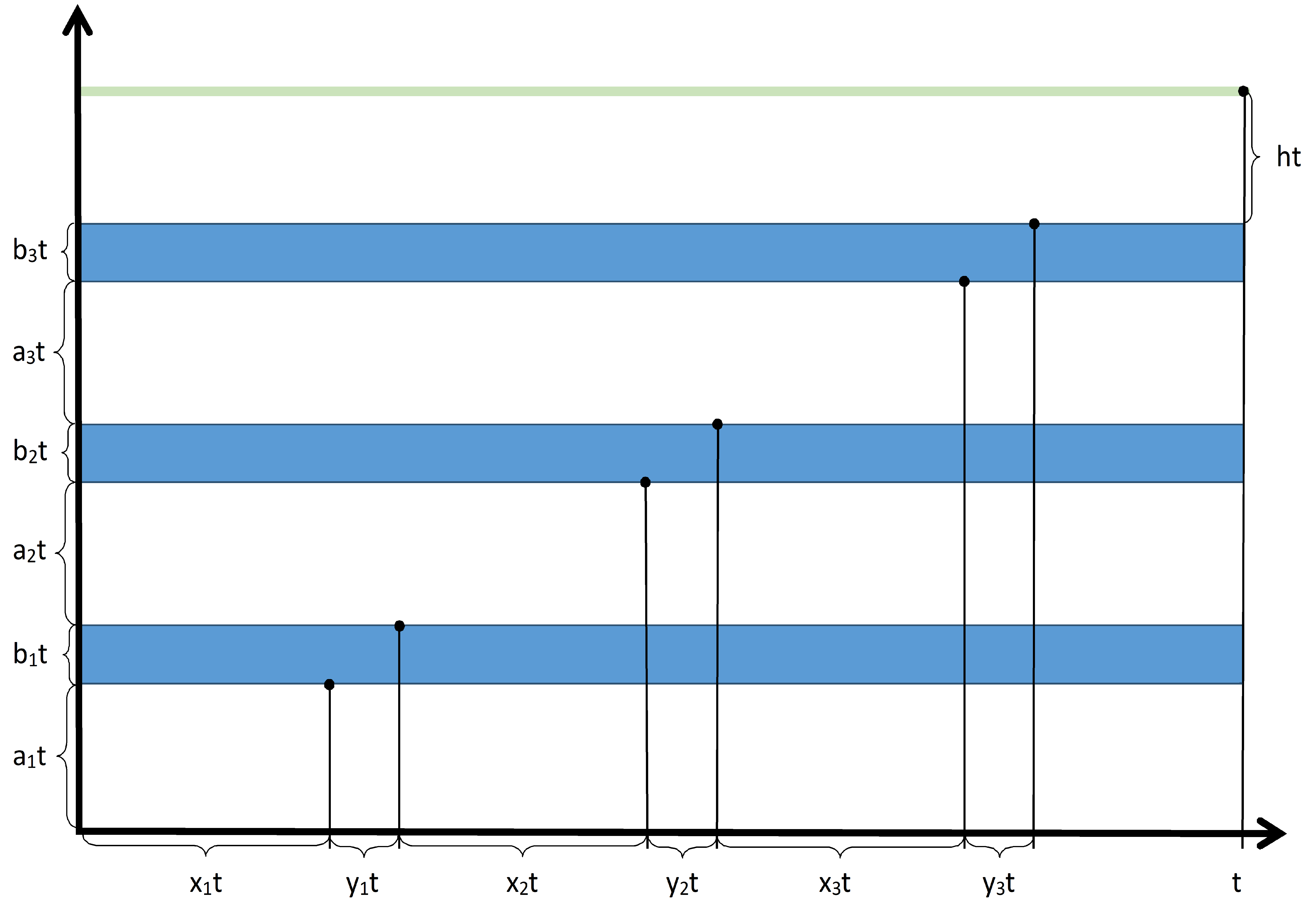
Figure 1. This is an example of $\ell=3$ obstacles. The vertical axis shows space and the horizontal axis time. In the white intervals of size $a_{i}t$ and in $[\sum_{i=1}^{\ell}(a_{i}+b_{i})t,\infty)$ and $(-\infty,0)$, BBM among obstacles branches at rate $1$. In the blue intervals of size $b_{i}t$, it does not branch. The green line is at height $\sum_{i=1}^{\ell}(a_{i}+b_{i})t+ht$.

Remark 1.2.

BBM among obstacles can also be related to F-KPP equations with a spatially inhomogeneous reaction term. Such F-KPP equations have recently been studied in e.g. [16, 23]. Note that the model in Definition 1.1 corresponds to a setting where the inhomogeneity also depends on the total time horizons.

1.2. Main result

In this article, we derive the first order of the position of the maximal particle at time $t$, depending on $a_{i},b_{i},i\leq\ell$.

To state the main result, we first introduce some notation.

We define indices $s_{0}<s_{1}<...<s_{n}<s_{n+1}$ via $s_{0}=0$, $s_{n+1}=\ell$ and

$$\{s_{1},\!...,s_{n}\}=\left\{m\in\{1,...,\ell-1\}:\frac{\sum_{i=1}^{m}b_{i}}{\sum_{i=1}^{m}a_{i}}\geq\frac{\sum_{i=m+1}^{\ell}b_{i}}{\sum_{i=m+1}^{\ell}a_{i}}\right\}.$$ (1.3)

We use them to define indices $0=u_{0}^{*}<u_{1}^{*}<...<u_{n^{*}}^{*}<u_{n^{*}+1}^{*}=\ell$ iteratively.

Definition 1.3.

Let $u_{0}^{*}=0$. Given $u_{0}^{*},\!...,u_{\tilde{i}}^{*}$, we define $u_{\tilde{i}+1}^{*}$ as follows. We pick $\tilde{j}=\inf\{j:s_{j}>u_{\tilde{i}}^{*}\}$, the index of the next candidate. Then we pick, if it exists, $\hat{j}=\sup\{j:j\in\{\tilde{j}+1,\!...,n+1\}\text{ and }\eqref{next ui*}\}$, the largest index such that

$$\frac{\sum_{i=u_{\tilde{i}}^{*}+1}^{s_{j}}b_{i}}{\sum_{i=u_{\tilde{i}}^{*}+1}^{s_{j}}a_{i}}<\frac{\sum_{i=s_{j}+1}^{s_{\hat{j}}}b_{i}}{\sum_{i=s_{j}+1}^{s_{\hat{j}}}a_{i}}\text{ for all }j=\tilde{j},\!...,\hat{j}-1,$$ (1.4)

and set $u_{\tilde{i}+1}^{*}=s_{\hat{j}}$. If such $\hat{j}$ does not exist, we set $u_{\tilde{i}+1}^{*}=s_{\tilde{j}}$. We iterate this until $s_{\tilde{j}}=\ell$ or $s_{\hat{j}}=\ell$.

For $m=u_{i}^{*}+1,\!...,u_{i+1}^{*}$ and $i=0,\!...,n^{*}$, we define

$$\tilde{c}_{i} =\frac{\left(\sum_{j=u_{i}^{*}+1}^{u_{i+1}^{*}}b_{j}\right)^{2}}{2\left(\sum_{j=u_{i}^{*}+1}^{u_{i+1}^{*}}a_{j}\right)^{2}}\quad\mbox{and}\quad f(\tilde{c}_{i})=\sqrt{\frac{1+\tilde{c}_{i}}{2}+\sqrt{\frac{\tilde{c}_{i}^{2}}{4}+\tilde{c}_{i}}}.$$ (1.5)

Moreover, let

$$x_{m}^{*} =a_{m}f(\tilde{c}_{i})\quad\mbox{and}\quad y_{m}^{*}=\frac{b_{m}}{2\frac{\sum_{j=u_{i}^{*}+1}^{u_{i+1}^{*}}a_{j}}{\sum_{j=u_{i}^{*}+1}^{u_{i+1}^{*}}b_{j}}\left(f(\tilde{c}_{i})-\frac{1}{2f(\tilde{c}_{i})}\right)}.$$ (1.6)

The main result is the following.

Theorem 1.4.

Let $(a_{i},b_{i})_{i=1}^{\ell}$ be some obstacle landscape such that $\sum_{i=1}^{\ell}(x_{i}^{*}+y_{i}^{*})\leq 1$. Then we have, almost surely,

$$\lim\limits_{t\to\infty}\frac{\max_{k\leq n(t)}X_{k}(t)}{t}=\sum_{i=1}^{\ell}(a_{i}+b_{i})+h^{*}$$ (1.7)

with $h^{*}=\sqrt{2}\left(1-\sum_{i=1}^{\ell}(x_{i}^{*}+y_{i}^{*})\right)$.

Remark 1.5.

Note that the suppression of branching in intervals of sizes proportional to $t$, lowers the linear order of the maximal particle position. However, the total number of particles is still of the same orderas in standard BBM, as branching is not suppressed in a neighbourhood around zero (whose size is also proportional to $t$). This is in contrast to other models in which branching is reduced, see for example [14, 11] or where particles are absorbed [6, 4, 5, 29] .

Under the additional assumption

$$\frac{\sum_{i=1}^{m}b_{i}}{\sum_{i=1}^{m}a_{i}}<\frac{\sum_{i=m+1}^{\ell}b_{i}}{\sum_{i=m+1}^{\ell}a_{i}}\text{ for all }m=1,\!...,\ell-1.$$ (1.8)

the statement of Theorem 1.4 simplifies to the following.

Corollary 1.6.

Assume (1.8). Then

$$\sum_{i=1}^{\ell}\left(x_{i}^{*}+y_{i}^{*}\right)=\sum_{i=1}^{\ell}a_{i}f(\tilde{c}_{0})+\frac{\left(\sum_{i=1}^{\ell}b_{i}\right)^{2}}{2\sum_{i=1}^{\ell}a_{i}\left(f(\tilde{c}_{0})-\frac{1}{2f(\tilde{c}_{0})}\right)}$$ (1.9)

and $\lim\limits_{t\to\infty}\max_{k\leq n(t)}X_{k}(t)/t$ is almost surely equal to

$$\sum_{i=1}^{\ell}(a_{i}+b_{i})+\sqrt{2}\left(1-\sum_{i=1}^{\ell}a_{i}f(\tilde{c}_{0})-\frac{\left(\sum_{i=1}^{\ell}b_{i}\right)^{2}}{2\sum_{i=1}^{\ell}a_{i}\left(f(\tilde{c}_{0})-\frac{1}{2f(\tilde{c}_{0})}\right)}\right).$$ (1.10)

Note that under Assumption (1.8), we have $\{u_{0}^{*},u_{1}^{*},\!...,u_{n+1}^{*}\}=\{0,\ell\}$.

Remark 1.7.

Note that (1.9) only depends on $\sum_{i=1}^{\ell}a_{i}$, the whole size of the $\ell$ branching areas, and $\sum_{i=1}^{\ell}b_{i}$, the whole size of all obstacles as $x_{m}^{*}$ and $y_{m}^{*}$ are proportional to $a_{m}$, respectively $b_{m}$ (at least for given $\sum_{i=1}^{\ell}a_{i}$ and $\sum_{i=1}^{\ell}b_{i}$).

We can interpret the overall costs of the first $m$ obstacles as the ratio between their size, $\sum_{i=1}^{m}b_{i}$, and the size of the corresponding branching areas, $\sum_{i=1}^{m}a_{i}$. The same applies to the last $\ell-m$ obstacles. Then assumption (1.8) says that the obstacles that a particle has already passed are always less expensive than the obstacles ahead. Hence, it will be worth it to wait for a certain amount of particles above an obstacle to cope with the more expensive remaining way and the minimal time a particle needs to get above all obstacles is

$$\left(\sum_{i=1}^{\ell}a_{i}f(\tilde{c}_{0})+\frac{\left(\sum_{i=1}^{\ell}b_{i}\right)^{2}}{2\sum_{i=1}^{\ell}a_{i}\left(f(\tilde{c}_{0})-\frac{1}{2f(\tilde{c}_{0})}\right)}\right)t.$$ (1.11)

If Assumption (1.8) does not hold, the optimal strategy requires only order one many particles above the $u_{i}^{*}$-th obstacle. Furthermore, we see that between the indices $u_{i}^{*}$ and $u_{i+1}^{*}$, the assumption

$$\frac{\sum_{j=u_{i}^{*}+1}^{m}b_{j}}{\sum_{j=u_{i}^{*}+1}^{m}a_{j}}<\frac{\sum_{j=m+1}^{u_{i+1}^{*}}b_{j}}{\sum_{j=m+1}^{u_{i+1}^{*}}a_{j}}\text{ for all }m=u_{i}^{*}+1,\!...,u_{i+1}^{*}-1$$ (1.12)

of late expensive obstacles holds. Hence, we apply (1.9) to each "block". In particular, the minimal time to get above all obstacles is

$$\sum_{i=1}^{\ell}(x_{i}^{*}+y_{i}^{*})t=\sum_{i=0}^{n^{*}}\left(\sum_{j=u_{i}^{*}+1}^{u_{i+1}^{*}}a_{j}f(\tilde{c}_{i})+\frac{\left(\sum_{j=u_{i}^{*}+1}^{u_{i+1}^{*}}b_{j}\right)^{2}}{2\sum_{j=u_{i}^{*}+1}^{u_{i+1}^{*}}a_{j}\left(f(\tilde{c}_{i})-\frac{1}{2f(\tilde{c}_{i})}\right)}\right)t,$$ (1.13)

the sum of the minimal times the particle needs to cross each block. The time to go through one block as fast as possible depends only on the size of all obstacles in this block, $\sum_{j=u_{i}^{*}+1}^{u_{i+1}^{*}}b_{j}$, and the size of all branching areas in this block, $\sum_{j=u_{i}^{*}+1}^{u_{i+1}^{*}}a_{j}$. Within this block, the optimal times (1.6) are proportional to the size of the corresponding branching area respectively obstacle.

Remark 1.8.

If (1.13) is strictly greater than $t$, we have, almost surely,

$$\lim\limits_{t\to\infty}\frac{\max_{k\leq n(t)}X_{k}(t)}{t}<\sum_{i=1}^{\ell}(a_{i}+b_{i}).$$ (1.14)

To identify the first order of the maximum in this case, one can proceed as follows. For $\hat{\ell}\in\{1,\!...,\ell-1\}$ and $b\in(0,b_{\hat{\ell}}]$, we define $\left(x_{1}^{*}\left(\hat{\ell},b\right),y_{1}^{*}\left(\hat{\ell},b\right),\!...,x_{\hat{\ell}}^{*}\left(\hat{\ell},b\right),y_{\hat{\ell}}^{*}\left(\hat{\ell},b\right)\right)$ for $\left(a_{1},b_{1},\!...,a_{\hat{\ell}-1},b_{\hat{\ell}-1},a_{\hat{\ell}},b\right)$ analogously to $(x_{1}^{*},y_{1}^{*},\!...,x_{\ell}^{*},y_{\ell}^{*})$ for $(a_{i},b_{i})_{i=1}^{\ell}$. Furthermore, we define $\hat{\ell}^{*}=\sup\left\{\hat{\ell}\in\{1,\!...,\ell-1\}:\sum_{i=1}^{\hat{\ell}}\left(x_{i}^{*}\left(\hat{\ell},b_{\hat{\ell}}\right)+y_{i}^{*}\left(\hat{\ell},b_{\hat{\ell}}\right)\right)\leq 1\right\}$, the number of the highest obstacle that can be crossed completely until time $t$. If $\sqrt{2}\left(1-\sum_{i=1}^{\hat{\ell}^{*}}\left(x_{i}^{*}\left(\hat{\ell}^{*},b_{\hat{\ell}^{*}}\right)+y_{i}^{*}\left(\hat{\ell}^{*},b_{\hat{\ell}^{*}}\right)\right)\right)\leq a_{\hat{\ell}^{*}+1}$, we have, almost surely,

$$\lim\limits_{t\to\infty}\frac{\max_{k\leq n(t)}X_{k}(t)}{t}=\sum_{i=1}^{\hat{\ell}^{*}}(a_{i}+b_{i})+\sqrt{2}\left(1-\sum_{i=1}^{\hat{\ell}^{*}}\left(x_{i}^{*}\left(\hat{\ell}^{*},b_{\hat{\ell}^{*}}\right)+y_{i}^{*}\left(\hat{\ell}^{*},b_{\hat{\ell}^{*}}\right)\right)\right).$$ (1.15)

If $\sqrt{2}\left(1-\sum_{i=1}^{\hat{\ell}^{*}}\left(x_{i}^{*}\left(\hat{\ell}^{*},b_{\hat{\ell}^{*}}\right)+y_{i}^{*}\left(\hat{\ell}^{*},b_{\hat{\ell}^{*}}\right)\right)\right)>a_{\hat{\ell}^{*}+1}$, we define
$b^{*}=\sup\left\{b\in\Big{(}0,b_{\hat{\ell}^{*}+1}\Big{]}:\sum_{i=1}^{\hat{\ell}^{*}+1}\left(x_{i}^{*}\left(\hat{\ell}^{*}+1,b\right)+y_{i}^{*}\left(\hat{\ell}^{*}+1,b\right)\right)\leq 1\right\}$ and have, almost surely,

$$\lim\limits_{t\to\infty}\frac{\max_{k\leq n(t)}X_{k}(t)}{t}=\sum_{i=1}^{\hat{\ell}^{*}}(a_{i}+b_{i})+a_{\hat{\ell}^{*}+1}+b^{*}.$$ (1.16)

Outline of the paper. In Section 2, we state some preparatory lemmas, which we need later on. In Section 3, we explain how Theorem 1.4 is connected to solving an optimization problem over possible paths and solve this optimization problem. In Section 4, we prove Theorem 1.4.

2. Preparatory estimates and notation

In this section, we introduce some notation, collect some Gaussian estimates and properties of standard BBM, which we need later.

We use the following notation in the remainder. For functions $f:[0,\infty)\to\mathbb{R}$ and $g:[0,\infty)\to\mathbb{R}$, we write
$f(t)\lesssim g(t)$ if $f(t)<g(t)e^{\delta t}$, as $t\to\infty$, for all $\delta>0$,
$f(t)\gtrsim g(t)$ if $f(t)>g(t)e^{-\delta t}$, as $t\to\infty$, for all $\delta>0$
and $f(t)\approx g(t)$ if $f(t)\lesssim g(t)$ and $f(t)\gtrsim g(t)$.

We need the following elementary Gaussian estimates.

Lemma 2.1.

Let $y>0$ and $b>0$ be some constants, $X\sim\mathcal{N}(0,yt)$ and $Y\sim\mathcal{N}(0,1)$ some centered Gaussian random variables and $f:[0,\infty)\to[0,\infty)$ and $g:[0,\infty)\to[0,\infty)$ some functions with $f(t)=o(t)$ respectively $g(t)=o(t)$. Then we have

$$\mathbb{P}\left(X\in\left[bt-g(t),bt+f(t)\right]\right)\approx e^{-\frac{b^{2}t}{2y}},$$ (2.1)

$$\mathbb{P}\left(X>bt\pm f(t)\right)\lesssim e^{-\frac{b^{2}t}{2y}},$$ (2.2)

$$\mathbb{P}\left(Y>t^{\frac{3}{4}}\right)\lesssim e^{-\frac{t^{\frac{3}{2}}}{2}}.$$ (2.3)

Proof.

(2.2) and (2.3) follow immediately from Gaussian tail estimates. For (2.1), we note that the probability in the right hand side  of (2.1) is bounded from above by $\mathbb{P}\left(X\geq bt-g(t)\right)$. Then (2.1) follows again from a Gaussian tail estimate. ∎

Moreover, we need an estimate on the size of the level sets of a standard binary BBM. For $x\in(0,1)$ and $a>0$, we define

$$\widehat{Z}_{a}(xt) =\#\left\{k\leq\hat{n}(xt):\widehat{X}_{k}(xt)\geq at\right\},$$ (2.4)

$$\widehat{Z}_{a}^{>}(xt) =\#\left\{k\leq\hat{n}(xt):\widehat{X}_{k}(xt)\geq at\text{ and }\exists s\in[0,xt]:\widehat{X}_{k}(s)>\frac{a}{x}s+\delta t\right\},$$ (2.5)

$$\widehat{Z}_{a}^{<}(xt) =\#\left\{k\leq\hat{n}(xt):\widehat{X}_{k}(xt)\geq at\text{ and }\exists s\in[0,xt]:\widehat{X}_{k}(s)<\frac{a}{x}s-\delta t\right\}.$$ (2.6)

The next lemma can be essentially found in [[22], Theorem 1.1] and describes the asymptotic behaviour of $\widehat{Z}_{a}(xt)$.

Lemma 2.2.

For any $x\in(0,1)$ and $a>0$, we have

$$\mathbb{E}\left[\widehat{Z}_{a}(xt)\right]\approx\exp\left(xt-\dfrac{a^{2}t}{2x}\right).$$ (2.7)

For any $x\in(0,1)$ and $a\in(0,\sqrt{2}xt)$, we have, almost surely,

$$\lim\limits_{t\to\infty}\frac{\widehat{Z}_{a}(t)}{\mathbb{E}\left[\widehat{Z}_{a}(t)\right]}=M_{a}\quad\mbox{a.s.}$$ (2.8)

where $M_{a}$ is the almost sure limit, as $t\to\infty$, of the McKean’s martingale

$$M_{a}(t)=\sum_{k=1}^{\hat{n}(t)}\exp\left(-t\left(1+\frac{a^{2}}{2}\right)+a\widehat{X}_{k}(t)\right).$$ (2.9)

For any $x\in(0,1)$, $a\in(0,\sqrt{2}xt)$, $\delta>0$ and $\gamma\in(0,2\delta^{2}/x)$, there exists $C_{1}>0$ such that

$$\mathbb{P}\left(\widehat{Z}_{a}^{>}(xt)>\mathbb{E}\left[\widehat{Z}_{a}(xt)\right]e^{-\gamma t}\right)+\mathbb{P}\left(\widehat{Z}_{a}^{<}(xt)>\mathbb{E}\left[\widehat{Z}_{a}(xt)\right]e^{-\gamma t}\right)\lesssim e^{-C_{1}t}.$$ (2.10)

Proof.

It is well known that, by the many-to-one Lemma,

$$\mathbb{E}\left[\widehat{Z}_{a}(xt)\right]=\mathbb{E}\left[\sum_{k=1}^{\hat{n}(xt)}\mathbbm{1}_{\widehat{X}_{k}(xt)\geq at}\right]\approx\exp\left(xt-\dfrac{a^{2}t}{2x}\right).$$ (2.11)

In [[22], Theorem 1.1], (2.8) is shown.

To show (2.10), we proceed analogously to the proof of [[22], Lemma 2.3]. To bound

$$\mathbb{P}\left(\widehat{Z}_{a}^{>}(xt)>\mathbb{E}\left[\widehat{Z}_{a}(xt)\right]e^{-\gamma t}\right)$$ (2.12)

from above via Markov´s inequality, we compute the expectation of $\widehat{Z}_{a}^{>}(xt)$. By the many-to-one-formula and distinguishing according to the position at time $xt$, we get

$$\mathbb{E}\left[\widehat{Z}_{a}^{>}(xt)\right] =e^{xt}\int_{at}^{\infty}\mathbb{P}\left(\widehat{X}_{1}(xt)\in dy\right)\mathbb{P}\left(\exists s\in[0,xt]:\widehat{X}_{1}(s)>\frac{a}{x}s+\delta t\middle|\widehat{X}_{1}(xt)=y\right)$$ (2.13)

$$=e^{xt}\int_{at}^{\infty}\mathbb{P}\left(\widehat{X}_{1}(xt)\in dy\right)\mathbb{P}\left(\exists s\in[0,xt]:b(s)>l(s)\middle|\widehat{X}_{1}(xt)=y\right)$$ (2.14)

with $b(s)=\widehat{X}_{1}(s)-\frac{s}{xt}\widehat{X}_{1}(xt)$ and $l(s)=(a/x-y/(xt))s+\delta t$. Since $b(s)$ is a Brownian bridge of length $xt$, we compute

$$\mathbb{E}\left[\widehat{Z}_{a}^{>}(xt)\right] =e^{xt}\int_{at}^{\infty}\mathbb{P}\left(\widehat{X}_{1}(xt)\in dy\right)\exp\left(-2\frac{l(0)l(xt)}{xt}\right)$$ (2.15)

$$=e^{xt}\int_{at}^{\infty}\frac{1}{\sqrt{2\pi xt}}\exp\left(-\frac{\left(y-2\delta t\right)^{2}}{2xt}\right)\exp\left(-\frac{2\delta at}{x}\right)dy.$$ (2.16)

By Lemma 2.1, we have

$$\mathbb{E}\left[\widehat{Z}_{a}^{>}(xt)\right] \approx\exp\left(xt-\frac{\left(at-2\delta t\right)^{2}}{2xt}-\frac{2\delta at}{x}\right)=\exp\left(xt-\frac{a^{2}t}{2x}-\frac{2\delta^{2}t}{x}\right).$$ (2.17)

Finally, using Markov´s inequality, (2.17) and (2.7), we get

$$\mathbb{P}\left(\widehat{Z}_{a}^{>}(xt)>\mathbb{E}\left[\widehat{Z}_{a}(xt)\right]e^{-\gamma t}\right)\lesssim\exp\left(-\frac{2\delta^{2}t}{x}+\gamma t\right).$$ (2.18)

The exponent on the r.h.s of (2.18) is strictly negative for all $\gamma<2\delta^{2}/x$. Since $\mathbb{P}\left(\widehat{Z}_{a}^{>}(xt)>\mathbb{E}\left[\widehat{Z}_{a}(xt)\right]e^{-\gamma t}\right)$ can be bounded analogously, we have (2.10). ∎

3. An optimization problem

3.1. Optimization problem connected to Theorem 1.4

Our candidate for the first order of the maximum of BBM among obstacles is $\sum_{i=1}^{\ell}(a_{i}+b_{i})t+h^{*}t$, where $(h^{*})^{2}/2$ is the maximum of

$$\left(1-\sum_{i=1}^{\ell}(x_{i}+y_{i})\right)\left(\sum_{i=1}^{\ell}\left(x_{i}-\frac{a_{i}^{2}}{2x_{i}}-\frac{b_{i}^{2}}{2y_{i}}\right)+1-\sum_{i=1}^{\ell}(x_{i}+y_{i})\right)$$

$$=\left(1-\sum_{i=1}^{\ell}(x_{i}+y_{i})\right)\left(1-\sum_{i=1}^{\ell}\left(y_{i}+\frac{a_{i}^{2}}{2x_{i}}+\frac{b_{i}^{2}}{2y_{i}}\right)\right).$$ (3.1)

over the domain

$$D=\{(x_{1},y_{1},\!...,x_{\ell},y_{\ell})\in\mathbb{R}^{2\ell}:\eqref{domain1},\eqref{domain3},\eqref{domain4}\}$$ (3.2)

with conditions

$$\sum_{i=1}^{m}\left(x_{i}-\frac{a_{i}^{2}}{2x_{i}}-\frac{b_{i}^{2}}{2y_{i}}\right)\geq 0\text{ for all }m=1,\!...,\ell,$$ (3.3)

$$\sum_{i=1}^{\ell}(x_{i}+y_{i})\leq 1,$$ (3.4)

$$x_{i}>0\text{ and }y_{i}>0\text{ for all }i=1,\!...,\ell.$$ (3.5)

We show that the argmax of (3.1) over $D$ equals the argmax of (3.1) over

$$\hat{D}=\{(x_{1},y_{1},\!...,x_{\ell},y_{\ell})\in D:\eqref{domain1}\text{ holds with equality for }m=\ell\}.$$ (3.6)

We briefly explain the heuristics which lead to this optimization problem. Assume that we need time $x_{i}t$ to cross the $i$-th obstacle free area and time $y_{i}t$ to cross the $i$-th obstacle (see Figure 1). By Lemma 2.2, there are approximately $\exp(x_{1}t-a_{1}^{2}t/(2x_{1}))$ particles around $a_{1}t$ at time $x_{1}t$. This implies that there are approximately $\exp(x_{1}t-a_{1}^{2}t/(2x_{1})-b_{1}^{2}t/(2y_{1}))$ offsprings of these particles at height $(a_{1}+b_{1})t$ at time $(x_{1}+y_{1})t$. Iterating this idea, this suggests that approximately $\exp(Jt)$ with

$$J=\sum_{i=1}^{\ell}\left(x_{i}-\frac{a_{i}^{2}}{2x_{i}}-\frac{b_{i}^{2}}{2y_{i}}\right)+\left(1-\sum_{i=1}^{\ell}(x_{i}+y_{i})\right)-\frac{h^{2}}{2\left(1-\sum_{i=1}^{\ell}(x_{i}+y_{i})\right)}$$ (3.7)

particles spend approximately time $x_{i}t$ to cross the $i$-th obstacle free area and time $y_{i}t$ to cross the $i$-th obstacle and reach height $\sum_{i=1}^{\ell}(a_{i}+b_{i})t+ht$. By setting $J=0$, we get, for fixed $(x_{1},y_{1},\!...,x_{\ell},y_{\ell})$, the largest possible $h$ such that there is at least one particle following the strategy. Solving for $h^{2}/2$ gives (3.1).

Next, we find $(x_{1},y_{1},\!...,x_{\ell},y_{\ell})$ that maximize (3.1) under the additional constraint that such particles exist, which leads to the definition of the domain $D$. Condition (3.3) guarantees that our strategy has at least one particle (following the strategy) after the $m$-th obstacle at the desired time. Conditions (3.4) and (3.5) say that the total time is bounded from above by $t$ and the particles spend positive time in the $m$-th branching area respectively obstacle.

Equality in (3.3) for $m=\ell$ means there are order one many particles above all obstacles at time $\sum_{i=1}^{\ell}(x_{i}+y_{i})t$. Furthermore, (3.1) takes the form $(1-\sum_{i=1}^{\ell}(x_{i}+y_{i}))^{2}$, which is maximal if $\sum_{i=1}^{\ell}(x_{i}+y_{i})$ is minimal. That the argmax of (3.1) over $D$ equals the argmax of (3.1) over $\hat{D}$ means that the maximal particle at time $t$ is a descendant of one of the first particles above all obstacles.

In the remainder of this section, we solve the above optimization problem. We use this solution in the proof of Theorem 1.4 in Section 4, making the above heuristics precise.

3.2. Optimization over $\hat{D}$ under Assumption (1.8)

In this subsection, we find the argmin of $\sum_{i=1}^{\ell}(x_{i}+y_{i})$, and hence the argmax of (3.1), over $\hat{D}$ under the additional Assumption (1.8) of late expensive obstacles.

The idea for finding the optimum over $\hat{D}$ is the following. We assume that we have $\approx e^{c_{m-1}t}$ particles above the $(m-1)$-th obstacle at time $\sum_{i=1}^{m-1}(x_{i}+y_{i})t$. Then we choose $x_{m}$ and $y_{m}$ such that we get $\approx e^{c_{m}t}$ particles above the $m$-th obstacle as soon as possible. Afterwards, we optimize over $(c_{1},\!...,c_{\ell-1})$.

To formalize this, we define the following domains. For $m=1,\!...,\ell$, we define

$$D^{m}(c_{m-1},c_{m}) =\{(x_{m},y_{m})\in\mathbb{R}^{2}:\eqref{xmc domain1},\eqref{xmc domain3},\eqref{xmc domain4}\},$$ (3.8)

where

$$c_{m-1}+x_{m}-\frac{a_{m}^{2}}{2x_{m}}-\frac{b_{m}^{2}}{2y_{m}}=c_{m},$$ (3.9)

$$x_{m}+y_{m}\leq N,$$ (3.10)

$$x_{m}>0\text{ and }y_{m}>0,$$ (3.11)

where $N>1$ is some large constant and $c_{\ell}=c_{0}=0$.

Remark 3.1.

The constraints are motivated as follows: Starting with $\approx e^{c_{m-1}t}$ particles above the $(m-1)$-th obstacle and wanting $\approx e^{c_{m}t}$ particles above the $m$-th obstacle as soon as possible, means we want to minimize $x_{m}+y_{m}$ such that (3.9) holds. Condition (3.10) says, for technical reasons, that the total time is bounded from above by $Nt$.

As we let the branching Brownian motion run for a time $t$, we define

$$\widetilde{D} =\{(x_{1},y_{1},...,x_{\ell},y_{\ell})\in\mathbb{R}^{2\ell}:\eqref{domain3}\text{ holds and }$$

$$\qquad\qquad(x_{m},y_{m})\in D^{m}(c_{m-1},c_{m})\text{ for }m=1,...,\ell\}.$$ (3.12)

We have $c_{\ell}=0$, because (3.3) holds with equality for $m=\ell$, and $c_{0}=0$, because we start with one particle at the origin. The remaining $(c_{1},\!...,c_{\ell-1})$ should be in the domain $D^{c}=\{(c_{1},\!...,c_{\ell-1})\in\mathbb{R}^{\ell-1}:\eqref{cm domain1},\eqref{cm domain2}\}$ with conditions

$$c_{m}\geq 0\text{ for all }m=1,\!...,\ell-1,$$ (3.13)

$$\widetilde{D}\text{ is not empty.}$$ (3.14)

Condition (3.13) guarantees that there is at least $\approx 1$ particle above each obstacle. Condition (3.14) says that it is not impossible to find a strategy that corresponds to $(c_{1},\!...,c_{\ell-1})$.

The domains $\widetilde{D}$ and $D^{c}$ are constructed such that they are compatible with the domain $\hat{D}$ in the following sense.

Lemma 3.2.

Set, for $m=1,\!...,\ell$,

$$c_{m}=\sum_{i=1}^{m}\left(x_{i}-\frac{a_{i}^{2}}{2x_{i}}-\frac{b_{i}^{2}}{2y_{i}}\right),$$ (3.15)

and $c_{0}=0$. Then, $(x_{1},y_{1},\!...,x_{\ell},y_{\ell})\in\hat{D}$ if and only if $(c_{1},\!...,c_{\ell-1})\in D^{c}$ and $(x_{1},y_{1},\!...,x_{\ell},y_{\ell})\in\widetilde{D}$ hold.

Proof.

Let $(x_{1},y_{1},\!...,x_{\ell},y_{\ell})\in\hat{D}$. Equality in (3.3) for $m=\ell$ implies $c_{\ell}=0$. Condition (3.9) also holds by (3.15), condition (3.10) by (3.4) and condition (3.11) by (3.5). Hence, $(x_{m},y_{m})\in D^{m}(c_{m-1},c_{m})$ and, by (3.4), $(x_{1},y_{1},\!...,x_{\ell},y_{\ell})\in\widetilde{D}$. Since condition (3.13) holds by (3.3) and $\widetilde{D}$ is not empty, we finally get $(c_{1},\!...,c_{\ell-1})\in D^{c}$. The reverse direction works analogously. ∎

Lemma 3.3.

The domain $D^{c}$ is convex.

Proof.

Let $c^{0}=(c^{0}_{1},\!...,c^{0}_{\ell})$ and $c^{1}=(c^{1}_{1},\!...,c^{1}_{\ell})$ be in $D^{c}$ and $\alpha\in(0,1)$. Then there exist $(x^{0}_{1},y^{0}_{1},\!...,x^{0}_{\ell},y^{0}_{\ell})$ and $(x^{1}_{1},y^{1}_{1},\!...,x^{1}_{\ell},y^{1}_{\ell})$ such that, for all $m=1,\!...,\ell$ and $q\in\{0,1\}$,

$$c^{q}_{m-1}+x^{q}_{m}-\frac{a_{m}^{2}}{2x^{q}_{m}}-\frac{b_{m}^{2}}{2y^{q}_{m}}=c^{q}_{m},$$ (3.16)

$$x^{q}_{m}>0\text{ and }y^{q}_{m}>0,$$ (3.17)

$$\sum_{i=1}^{\ell}(x^{q}_{i}+y^{q}_{i})\leq 1.$$ (3.18)

We have to show that $\alpha c^{0}+(1-\alpha)c^{1}\in D^{c}$. Condition (3.13) is clear. Let $x_{m}=\alpha x^{0}_{m}+(1-\alpha)x^{1}_{m}$. By (3.17), we have $x_{m}>0$ . Choosing

$$y_{m}=\frac{b_{m}^{2}}{2\left(\alpha(c^{0}_{m-1}-c^{0}_{m})+(1-\alpha)(c^{1}_{m-1}-c^{1}_{m})+\alpha x^{0}_{m}+(1-\alpha)x^{1}_{m}-\frac{a_{m}^{2}}{2(\alpha x^{0}_{m}+(1-\alpha)x^{1}_{m})}\right)},$$ (3.19)

implies that

$$\alpha c^{0}_{m-1}+(1-\alpha)c^{1}_{m-1}+\alpha x^{0}_{m}+(1-\alpha)x^{1}_{m}-\frac{a_{m}^{2}}{2(\alpha x^{0}_{m}+(1-\alpha)x^{1}_{m})}-\frac{b_{m}^{2}}{2y_{m}}=\alpha c^{0}_{m}+(1-\alpha)c^{1}_{m}.$$ (3.20)

Since $x-a_{m}^{2}/(2x)$ is concave in $x$, the denominator of (3.19) is bounded from below by

$$2\alpha\left(c^{0}_{m-1}-c^{0}_{m}+x^{0}_{m}-\frac{a_{m}^{2}}{2x^{0}_{m}}\right)+2(1-\alpha)\left(c^{1}_{m-1}-c^{1}_{m}+x^{1}_{m}-\frac{a_{m}^{2}}{2x^{1}_{m}}\right),$$ (3.21)

which is strictly positive by (3.16) and (3.17). Hence, $y_{m}>0$. By concavity of $x-a_{m}^{2}/(2x)$ and convexity of $1/x$, we can bound $y_{m}$ from above

$$y_{m} \leq\frac{b_{m}^{2}}{2\left(\alpha(c^{0}_{m-1}-c^{0}_{m}+x^{0}_{m}-\frac{a_{m}^{2}}{2x^{0}_{m}})+(1-\alpha)(c^{1}_{m-1}-c^{1}_{m}+x^{1}_{m}-\frac{a_{m}^{2}}{2x^{1}_{m}})\right)}$$ (3.22)

$$\leq\alpha y^{0}_{m}+(1-\alpha)y^{1}_{m},$$ (3.23)

by (3.16). Hence, we have

$$\sum_{i=1}^{\ell}(x_{i}+y_{i})\leq\alpha\sum_{i=1}^{\ell}(x^{0}_{i}+y^{0}_{i})+(1-\alpha)\sum_{i=1}^{\ell}(x^{1}_{i}+y^{1}_{i}),$$ (3.24)

which is less or equal to $1$ by (3.18). ∎

Proposition 3.4 shows existence and uniqueness of the best strategy in $\widetilde{D}$ that gets $\approx e^{c_{m}t}$ particles above the $m$-th obstacle given $\approx e^{c_{m-1}t}$ particles above the $(m-1)$-th obstacle. Furthermore, it shows that the argmin satisfies some first order condition. Let $D^{m}_{x}(c_{m-1},c_{m})=\{x\in\mathbb{R}:(x,y)\in D^{m}(c_{m-1},c_{m})\text{ for some }y\in\mathbb{R}\}$.

Proposition 3.4.

Let $(c_{1},\!...,c_{\ell-1})\in D^{c}$. Then there exists exactly one $(x_{1}^{c},y_{1}^{c},\!...,x_{\ell}^{c},y_{\ell}^{c})$ in $\widetilde{D}$ such that $(x_{m}^{c},y_{m}^{c})$ minimizes $x_{m}+y_{m}$ over $D^{m}(c_{m-1},c_{m})$ for all $m=1,...,\ell$. The component $x_{m}^{c}$ is the largest real solution of

$$\frac{b_{m}^{2}}{2\left(c_{m-1}+x_{m}^{c}-\frac{a_{m}^{2}}{2x_{m}^{c}}-c_{m}\right)^{2}}=\frac{1}{1+\frac{a_{m}^{2}}{2(x_{m}^{c})^{2}}}$$ (3.25)

and the only solution of (3.25) in $D^{m}_{x}(c_{m-1},c_{m})$. Moreover, $x_{m}^{c}$ is not a boundary point of $D^{m}_{x}(c_{m-1},c_{m})$.

Proof.

Solving (3.9) for $y_{m}$ gives

$$y_{m}=\frac{b_{m}^{2}}{2\left(c_{m-1}+x_{m}-\frac{a_{m}^{2}}{2x_{m}}-c_{m}\right)}.$$ (3.26)

Hence, we need to minimize

$$x_{m}+\frac{b_{m}^{2}}{2\left(c_{m-1}+x_{m}-\frac{a_{m}^{2}}{2x_{m}}-c_{m}\right)}$$ (3.27)

such that (3.10) and (3.11) hold. Differentiating (3.27) with respect to $x_{m}$ gives the first order condition

$$1-\frac{b_{m}^{2}}{2\left(c_{m-1}+x_{m}-\frac{a_{m}^{2}}{2x_{m}}-c_{m}\right)^{2}}\left(1+\frac{a_{m}^{2}}{2x_{m}^{2}}\right)=0.$$ (3.28)

The second derivative of (3.27) with respect to $x_{m}$ equals

$$\frac{b_{m}^{2}}{\left(c_{m-1}+x_{m}-\frac{a_{m}^{2}}{2x_{m}}-c_{m}\right)^{3}}\left(1+\frac{a_{m}^{2}}{2x_{m}^{2}}\right)^{2}+\frac{b_{m}^{2}}{2\left(c_{m-1}+x_{m}-\frac{a_{m}^{2}}{2x_{m}}-c_{m}\right)^{2}}\left(\frac{a_{m}^{2}}{x_{m}^{3}}\right),$$ (3.29)

which is strictly positive. Hence, (3.27) is strictly convex in $D^{m}_{x}(c_{m-1},c_{m})$ with respect to $x_{m}$ and has a unique minimizer in the closure of $D^{m}_{x}(c_{m-1},c_{m})$.

Now, suppose $x_{m}^{c}\in\partial D^{m}_{x}(c_{m-1},c_{m})$. Within the boundary, $x_{m}\to 0$ or $y_{m}\to 0$ would contradict (3.9) because $x_{m}\leq N$ is not able to compensate $a_{m}^{2}/(2x_{m})\to\infty$ or $b_{m}^{2}/(2y_{m})\to\infty$. Therefore, only equality in (3.10) is relevant. Hence, the minimum of $x_{m}+y_{m}$ over the closure of $D^{m}(c_{m-1},c_{m})$ would be $N$. But then the minimum of $\sum_{i=1}^{\ell}(x_{i}+y_{i})$ over $(x_{1},y_{1},\!...,x_{\ell},y_{\ell})$ such that $(x_{m},y_{m})\in D^{m}(c_{m-1},c_{m})$ for all $m=1,...,\ell$ would be at least $N>1$. In this case, (3.4) could not hold. Consequently, $\widetilde{D}$ would be empty, which contradicts $(c_{1},\!...,c_{\ell-1})\in D^{c}$.

Hence, $x_{m}^{c}$ has to be in the interior of $D^{m}_{x}(c_{m-1},c_{m})$, i.e. $x_{m}^{c}$ is a critical point and satisfies (3.28), which implies (3.25). Moreover, $\sum_{i=1}^{\ell}(x_{i}^{c}+y_{i}^{c})\leq 1$ has to be true, which implies $(x_{1}^{c},y_{1}^{c},\!...,x_{\ell}^{c},y_{\ell}^{c})\in\widetilde{D}$.

If $x_{m}^{c}$ was not the largest real solution of (3.25), we could choose $N$ so large that also this largest solution is in $D_{m}^{x}$. This would be a contradiction because, by strict convexity of (3.27), $x_{m}^{c}$ is the only critical point in $D_{m}^{x}$. ∎

In Corollary 3.5, we show the monotonicity of $x_{m}^{c}$ and $x_{m+1}^{c}$ in $c_{m}$.

Corollary 3.5.

For all $(c_{1},\!...,c_{\ell})$ in the interior of $D^{c}$, we have $\frac{\partial}{\partial c_{m}}x_{m}^{c}\equiv(x_{m}^{c})^{\prime}$ exists and is $\geq 0$. Moreover, $\frac{\partial}{\partial c_{m}}x_{m+1}^{c}\equiv(x_{m+1}^{c})^{\prime}$ exists and is $\leq 0$.

Proof.

Let $(c_{1},\!...,c_{\ell})$ be in the interior of $D^{c}$. We defer the proof of the differentiability of $x_{m}$ and $x_{m+1}$ with respect to $c_{m}$ to Appendix A, see Lemma A.8. To prove $(x_{m}^{c})^{\prime}\geq 0$, we show that $x_{m}^{c}$ is increasing in $c_{m}$. When increasing $c_{m}$, the l.h.s of (3.25) gets larger. As $x-a_{m}^{2}/(2x)$ is increasing in $x$ and $a_{m}^{2}/(2x^{2})$ is decreasing, $x_{m}^{c}$ increases in order to satisfy (3.25).

Similarly, we show that $x_{m+1}^{c}$ is decreasing in $c_{m}$ and hence $(x_{m+1}^{c})^{\prime}\leq 0$. The first order condition for $x_{m+1}^{c}$ has the form

$$\frac{b_{m+1}^{2}}{2\left(c_{m}+x_{m+1}^{c}-\frac{a_{m+1}^{2}}{2x_{m+1}^{c}}-c_{m+1}\right)^{2}}=\frac{1}{1+\frac{a_{m+1}^{2}}{2(x_{m+1}^{c})^{2}}}.$$ (3.30)

Now, the l.h.s of (3.30) gets smaller when increasing $c_{m}$. As $x-a_{m+1}^{2}/(2x)$ is increasing in $x$ and $a_{m+1}^{2}/(2x^{2})$ is decreasing, $x_{m+1}^{c}$ needs to be smaller in order to satisfy (3.30). ∎

Proposition 3.6.

If $\hat{D}$ is not empty and assumption (1.8) holds, then there is exactly one $(c_{1}^{*},\!...,c_{\ell-1}^{*})\in D^{c}$ that minimizes

$$\sum_{m=1}^{\ell}\left(x_{m}^{c}+\frac{b_{m}^{2}}{2\left(c_{m-1}+x_{m}^{c}-\frac{a_{m}^{2}}{2x_{m}^{c}}-c_{m}\right)}\right).$$ (3.31)

This argmin is given by

$$c_{m}^{*} =\frac{\big{(}\sum_{i=1}^{m}a_{i}\big{)}\big{(}\sum_{i=m+1}^{\ell}b_{i}\big{)}-\big{(}\sum_{i=1}^{m}b_{i}\big{)}\big{(}\sum_{i=m+1}^{\ell}a_{i}\big{)}}{\sum_{i=1}^{\ell}b_{i}}\left(f(\tilde{c})-\frac{1}{2f(\tilde{c})}\right)$$ (3.32)

with

$$\tilde{c}=\frac{\left(\sum_{i=1}^{\ell}b_{i}\right)^{2}}{2\left(\sum_{i=1}^{\ell}a_{i}\right)^{2}}\quad\text{and}\quad f(\tilde{c}) =\sqrt{\dfrac{1+\tilde{c}}{2}+\sqrt{\frac{\tilde{c}^{2}}{4}+\tilde{c}}}.$$ (3.33)

The corresponding optimal times are given by

$$x_{m}^{c} =a_{m}f(\tilde{c})\quad\mbox{and}\quad y_{m}^{c}=\frac{b_{m}}{2\frac{\sum_{i=1}^{\ell}a_{i}}{\sum_{i=1}^{\ell}b_{i}}\left(f(\tilde{c})-\frac{1}{2f(\tilde{c})}\right)},$$ (3.34)

for $m=1,\dots,\ell$.

Assumption (1.8) of late expensive obstacles ensures that the optimal $c_{m}^{*}$ is strictly positive. Note that

$$f(\tilde{c})>\frac{1}{\sqrt{2}},$$ (3.35)

because (3.35) is equivalent to $\tilde{c}+\sqrt{\tilde{c}^{2}+2\tilde{c}}>0$, which is true by $\tilde{c}>0$.

Lemma 3.7.

The system of linear equations

$$c_{m}=\frac{b_{m+1}a_{m}-b_{m}a_{m+1}}{b_{m}+b_{m+1}}\left(\dfrac{x_{1}^{c}}{a_{1}}-\frac{a_{1}}{2x_{1}^{c}}\right)+\dfrac{b_{m+1}}{b_{m}+b_{m+1}}c_{m-1}+\dfrac{b_{m}}{b_{m}+b_{m+1}}c_{m+1}$$ (3.36)

for $m=1,\!...,\ell-1$ has exactly one solution, which is given by

$$c_{m}=\frac{\big{(}\sum_{i=1}^{m}a_{i}\big{)}\big{(}\sum_{i=m+1}^{\ell}b_{i}\big{)}-\big{(}\sum_{i=1}^{m}b_{i}\big{)}\big{(}\sum_{i=m+1}^{\ell}a_{i}\big{)}}{\sum_{i=1}^{\ell}b_{i}}\left(\dfrac{x_{1}^{c}}{a_{1}}-\frac{a_{1}}{2x_{1}^{c}}\right).$$ (3.37)

Proof.

The corresponding matrix $(a_{m,j})_{m,j=1}^{\ell-1}$, with
$a_{m,m-1}=-b_{m+1}/(b_{m}+b_{m+1})$ for $m=2,\!...,\ell-1$,
$a_{m,m}=1$ for $m=1,\!...,\ell-1$,
$a_{m,m+1}=-b_{m}/(b_{m}+b_{m+1})$ for $m=1,\!...,\ell-2$ and
$a_{m,j}=0$ else, has full rank. To prove this, one notes that the $m$-th diagonal entry after Gaussian forward elimination is given by

$$\frac{b_{m}\sum_{i=1}^{m+1}b_{i}}{(b_{m}+b_{m+1})\sum_{i=1}^{m}b_{i}},$$ (3.38)

which can be checked by induction. As the expression (3.38) is $\in(0,1)$ for all $m=1,\!...,\ell-1$, the matrix has full rank and the system of equations (3.36) has at most one solution. Plugging (3.37) into (3.36), one checks that it is indeed a solution. ∎

Lemma 3.8.

Assume $(c_{1},\!...,c_{\ell-1})\in D^{c}$ and $c_{m}$ satisfies

$$c_{m}=\frac{\big{(}\sum_{i=1}^{m}a_{i}\big{)}\big{(}\sum_{i=m+1}^{\ell}b_{i}\big{)}-\big{(}\sum_{i=1}^{m}b_{i}\big{)}\big{(}\sum_{i=m+1}^{\ell}a_{i}\big{)}}{\sum_{i=1}^{\ell}b_{i}}\left(\dfrac{x_{m}^{c}}{a_{m}}-\frac{a_{m}}{2x_{m}^{c}}\right),$$ (3.39)

for $m=1,...,\ell-1$. Then we have, for $m=1,\!...,\ell$,

$$x_{m}^{c} =a_{m}f(\tilde{c}),$$ (3.40)

$$y_{m}^{c} =\frac{b_{m}}{2\frac{\sum_{i=1}^{\ell}a_{i}}{\sum_{i=1}^{\ell}b_{i}}\left(f(\tilde{c})-\frac{1}{2f(\tilde{c})}\right)}$$ (3.41)

and $c_{m}$ also satisfies (3.32).

Proof.

Plugging (3.39) for $c_{m}$ into (3.25), the first order condition for $x_{m}$, we get

$$1+\frac{a_{m}^{2}}{2\left(x_{m}^{c}\right)^{2}}=\frac{2}{b_{m}^{2}}\Bigg{[}\frac{\big{(}\sum_{i=1}^{m-1}a_{i}\big{)}\big{(}\sum_{i=m}^{\ell}b_{i}\big{)}-\big{(}\sum_{i=1}^{m-1}b_{i}\big{)}\big{(}\sum_{i=m}^{\ell}a_{i}\big{)}}{\sum_{i=1}^{\ell}b_{i}}$$ (3.42)

$$+a_{m}-\frac{\big{(}\sum_{i=1}^{m}a_{i}\big{)}\big{(}\sum_{i=m+1}^{\ell}b_{i}\big{)}-\big{(}\sum_{i=1}^{m}b_{i}\big{)}\big{(}\sum_{i=m+1}^{\ell}a_{i}\big{)}}{\sum_{i=1}^{\ell}b_{i}}\Bigg{]}^{2}\left(\frac{x_{m}^{c}}{a_{m}}-\frac{a_{m}}{2x_{m}^{c}}\right)^{2}.$$ (3.43)

(3.42) is equivalent to

$$1+\frac{a_{m}^{2}}{2\left(x_{m}^{c}\right)^{2}}=\frac{2\left({\sum_{i=1}^{\ell}a_{i}}\right)^{2}\left(\frac{x_{m}^{c}}{a_{m}}-\frac{a_{m}}{2x_{m}^{c}}\right)^{2}}{\left({\sum_{i=1}^{\ell}b_{i}}\right)^{2}}.$$ (3.44)

Setting $z=x_{m}^{c}/a_{m}$ and $\tilde{c}=(b_{1}+...+b_{\ell})^{2}/(2(a_{1}+...+a_{\ell})^{2})$, we write (3.44) as

$$1+\frac{1}{2z^{2}}=\frac{1}{\tilde{c}}\left(z-\frac{1}{2z}\right)^{2},$$ (3.45)

which is equivalent to $0=z^{4}-(1+\tilde{c})z^{2}+1/4-\tilde{c}/2$. We have

$$\frac{\left(x_{m}^{c}\right)^{2}}{a_{m}^{2}}=z^{2} =\dfrac{1+\tilde{c}}{2}\text{ }^{+}_{-}\sqrt{\frac{\tilde{c}^{2}}{4}+\tilde{c}}.$$ (3.46)

As $x_{m}>0$, we only need to consider the positive root $\sqrt{(1+\tilde{c})/2-\sqrt{\tilde{c}^{2}/4+\tilde{c}}}$ . If $\sqrt{(1+\tilde{c})/2-\sqrt{\tilde{c}^{2}/4+\tilde{c}}}$ is in $D^{m}_{x}(c_{m-1},c_{m})$, this implies that it is in $D^{m}_{x}(c_{m-1},c_{m})$ too, for $N$ large enough. This would lead to a contradiction as there is only one solution of (3.25) in $D^{m}_{x}(c_{m-1},c_{m})$ by Proposition 3.4. Hence, we have (3.40), i.e. $x_{m}^{c}=a_{m}z=a_{m}f(\tilde{c})$ with

$$f(\tilde{c})=\sqrt{\dfrac{1+\tilde{c}}{2}+\sqrt{\frac{\tilde{c}^{2}}{4}+\tilde{c}}}.$$ (3.47)

Plugging (3.39) into (3.26), we get

$$y_{m}^{c}= \frac{b_{m}^{2}}{2}\times\Bigg{[}\frac{\big{(}\sum_{i=1}^{m-1}a_{i}\big{)}\big{(}\sum_{i=m}^{\ell}b_{i}\big{)}-\big{(}\sum_{i=1}^{m-1}b_{i}\big{)}\big{(}\sum_{i=m}^{\ell}a_{i}\big{)}}{\sum_{i=1}^{\ell}b_{i}}+a_{m}$$ (3.48)

$$-\frac{\big{(}\sum_{i=1}^{m}a_{i}\big{)}\big{(}\sum_{i=m+1}^{\ell}b_{i}\big{)}-\big{(}\sum_{i=1}^{m}b_{i}\big{)}\big{(}\sum_{i=m+1}^{\ell}a_{i}\big{)}}{\sum_{i=1}^{\ell}b_{i}}\Bigg{]}^{-1}\left(\frac{x_{m}^{c}}{a_{m}}-\frac{a_{m}}{2x_{m}^{c}}\right)^{-1}.$$

If we cancel all terms that arise with both signs, simplify the fraction and use (3.40), we get (3.41). That $c_{m}$ satisfies (3.32), follows by plugging (3.40) into (3.39). ∎

Proof of Proposition 3.6 .

Assume that the interior of $D^{c}$ is not empty. (At the end of this proof, we will justify that this assumption does not cause a loss of generality.) Taking the derivative of (3.31) with respect to $c_{m}$ gives the first order condition

$$\left(x_{m}^{c}\right)^{\prime}-\frac{b_{m}^{2}}{2\left(c_{m-1}+x_{m}^{c}-\frac{a_{m}^{2}}{2x_{m}^{c}}-c_{m}\right)^{2}}\left(\left(x_{m}^{c}\right)^{\prime}+\frac{a_{m}^{2}}{2\left(x_{m}^{c}\right)^{2}}\left(x_{m}^{c}\right)^{\prime}-1\right)+\left(x_{m+1}^{c}\right)^{\prime}\\ -\frac{b_{m+1}^{2}}{2\left(c_{m}+x_{m+1}^{c}-\frac{a_{m+1}^{2}}{2x_{m+1}^{c}}-c_{m+1}\right)^{2}}\left(1+\left(x_{m+1}^{c}\right)^{\prime}+\frac{a_{m+1}^{2}}{2\left(x_{m+1}^{c}\right)^{2}}\left(x_{m+1}^{c}\right)^{\prime}\right)=0.$$ (3.49)

By plugging (3.25) into (3.49), we obtain

$$0= \frac{1}{1+\frac{a_{m}^{2}}{2\left(x_{m}^{c}\right)^{2}}}-\frac{1}{1+\frac{a_{m+1}^{2}}{2\left(x_{m+1}^{c}\right)^{2}}}.$$ (3.50)

We note that (3.50) holds if and only if

$$\frac{a_{m}}{x_{m}^{c}}=\frac{a_{m+1}}{x_{m+1}^{c}}.$$ (3.51)

The second derivative of (3.31) with respect to $c_{m}$ equals

$$\frac{1}{\left(1+\frac{a_{m}^{2}}{2\left(x_{m}^{c}\right)^{2}}\right)^{2}}\frac{a_{m}^{2}}{\left(x_{m}^{c}\right)^{3}}\left(x_{m}^{c}\right)^{\prime}-\frac{1}{\left(1+\frac{a_{m+1}^{2}}{2\left(x_{m+1}^{c}\right)^{2}}\right)^{2}}\frac{a_{m+1}^{2}}{\left(x_{m+1}^{c}\right)^{3}}\left(x_{m+1}^{c}\right)^{\prime}$$ (3.52)

and is non-negative, because $\left(x_{m}^{c}\right)^{\prime}\geq 0$ and $\left(x_{m+1}^{c}\right)^{\prime}\leq 0$ by Corollary 3.5. Hence, (3.31) is weakly convex with respect to $c_{m}$ in the relevant domain $D^{c}$. We will see soon that (3.31) has exactly one critical point in $D^{c}$. Because of this uniqueness, the weak convexity of (3.31) and Lemmas 3.3 and A.7, the desired minimum has to be attained at this critical point.

If we combine (3.25) and (3.51), we see that the critical $(c_{1},\!...,c_{\ell-1})$ has to satisfy

$$\frac{b_{m}}{c_{m-1}+x_{m}^{c}-\frac{a_{m}^{2}}{2x_{m}^{c}}-c_{m}}=\frac{b_{m+1}}{c_{m}+x_{m+1}^{c}-\frac{a_{m+1}^{2}}{2x_{m+1}^{c}}-c_{m+1}}.$$ (3.53)

We solve this for $c_{m}$ and use (3.51) again to get the system of linear equations

$$c_{m}= \frac{b_{m+1}\left(c_{m-1}+x_{m}^{c}-\frac{a_{m}^{2}}{2x_{m}^{c}}\right)-b_{m}\left(x_{m+1}^{c}-\frac{a_{m+1}^{2}}{2x_{m+1}^{c}}-c_{m+1}\right)}{b_{m}+b_{m+1}}$$ (3.54)

$$= \frac{b_{m+1}a_{m}-b_{m}a_{m+1}}{b_{m}+b_{m+1}}\left(\dfrac{x_{1}^{c}}{a_{1}}-\frac{a_{1}}{2x_{1}^{c}}\right)+\dfrac{b_{m+1}}{b_{m}+b_{m+1}}c_{m-1}+\dfrac{b_{m}}{b_{m}+b_{m+1}}c_{m+1}$$ (3.55)

for $m=1,\!...,\ell-1$. By Lemma 3.7, the unique solution of (3.55) is given by (3.37). By (3.51), it also satisfies (3.39). Hence, our candidates for the optimal times are given in Lemma 3.8 with $c_{m}$ satisfying (3.32).

It remains to show that the candidate given by (3.32) is in $D^{c}$. First, $c_{m}\geq 0$ follows by (1.8) and (3.35). We prove that $\tilde{D}$ is not empty by showing that the candidate satisfying (3.40) and (3.41) is an element of $\tilde{D}$. Condition (3.9) holds by construction of $y_{m}^{c}$ via (3.26). Condition (3.11) follows by (3.35). To get (3.10) and in particular (3.4), we need

$$\sum_{i=1}^{\ell}(x_{i}^{c}+y_{i}^{c})=\sum_{i=1}^{\ell}a_{i}f(\tilde{c})+\frac{\left(\sum_{i=1}^{\ell}b_{i}\right)^{2}}{2\sum_{i=1}^{\ell}a_{i}\left(f(\tilde{c})-\frac{1}{2f(\tilde{c})}\right)}\leq 1.$$ (3.56)

If we already knew that (3.56) was true, we could argue as follows: The candidate given by (3.32) is in $D^{c}$ with optimal times (3.40) and (3.41). Furthermore, it is a critical point, because it satisfies (3.51) by (3.40). As already mentioned, uniqueness of this critical point and weak convexity of (3.31) imply that the argmin of (3.31) over $D^{c}$ is given by (3.32).

We show that (3.56) is indeed true. Therefore, we define the domain $\hat{D}^{n}=\{(x_{1},y_{1},\!...,x_{\ell},y_{\ell})\in\mathbb{R}^{2\ell}:\eqref{domain1},\sum_{i=1}^{\ell}(x_{i}+y_{i})\leq n,\eqref{domain4},\eqref{domain1}\text{ holds with equality for }m=\ell\}$. It is almost the same definition as for $\hat{D}$ but the total time is bounded from above by $nt$ instead of $t$. We choose $n>1$ so large that the candidate on the l.h.s of (3.56) is smaller than $n$ and $\hat{D}^{n}$ is not empty. (For example, choose $n$ as the maximum of the l.h.s of (3.56) and $\sum_{i=1}^{\ell}(2a_{i}+b_{i}^{2}/(3.5a_{i}))$. Then $\hat{D}^{n}$ is not empty because it contains $(2a_{1},b_{1}^{2}/(3.5a_{1}),\!...,2a_{\ell},b_{\ell}^{2}/(3.5a_{\ell}))$.)

Then all entire results in Subsection 3.2 carry over if we adapt the definition of $\widetilde{D}$ and ensure $N>n$ in (3.10). Hence, the minimum of $\sum_{i=1}^{\ell}(x_{i}+y_{i})$ over $\hat{D}^{n}$ is the l.h.s of (3.56). Since $\hat{D}$ is a subset of $\hat{D}^{n}$, we have

$$\min\left\{\sum_{i=1}^{\ell}(x_{i}+y_{i}):(x_{1},y_{1},\!...,x_{\ell},y_{\ell})\in\hat{D}\right\}\\ \geq\min\left\{\sum_{i=1}^{\ell}(x_{i}+y_{i}):(x_{1},y_{1},\!...,x_{\ell},y_{\ell})\in\hat{D}^{n}\right\}.$$ (3.57)

By (3.4), this implies that $\hat{D}$ is not empty if and only if (3.56) is true. Since we assumed non-emptiness of $\hat{D}$, the claim follows. (Looking at $\hat{D}^{n}$ also justifies that we can assume non emptiness of the interior of $D^{c}$ without a loss of generality.) ∎

Corollary 3.9.

For any obstacle landscape $(a_{i},{b}_{i})_{i=1}^{\ell}$ satisfying assumption (1.8), the domain $\hat{D}$ is not empty if and only if

$$\sum_{i=1}^{\ell}a_{i}f(\tilde{c})+\frac{\left(\sum_{i=1}^{\ell}b_{i}\right)^{2}}{2\sum_{i=1}^{\ell}a_{i}\left(f(\tilde{c})-\frac{1}{2f(\tilde{c})}\right)}\leq 1.$$ (3.58)

The main result of this subsection is the following.

Theorem 3.10.

If $\hat{D}$ is not empty and assumption (1.8) holds, then the maximum of (3.1) over $\hat{D}$ equals $(h^{*})^{2}/2$ with

$$h^{*} =\sqrt{2}\left(1-\sum_{i=1}^{\ell}(x_{i}^{*}+y_{i}^{*})\right)$$ (3.59)

$$=\sqrt{2}\left(1-\sum_{i=1}^{\ell}a_{i}f(\tilde{c})-\frac{\left(\sum_{i=1}^{\ell}b_{i}\right)^{2}}{2\sum_{i=1}^{\ell}a_{i}\left(f(\tilde{c})-\frac{1}{2f(\tilde{c})}\right)}\right).$$ (3.60)

Proof.

The argmax of (3.1) over $\hat{D}$ equals the argmin of $\sum_{i=1}^{\ell}(x_{i}+y_{i})$ over $\hat{D}$. By Lemma 3.2 and Proposition 3.4, this is equivalent to minimizing $\sum_{i=1}^{\ell}(x_{i}^{c}+y_{i}^{c})$ over $D^{c}$. By Proposition 3.6, this argmin consists of the optimal times in Lemma 3.8. ∎

3.3. Optimization over $\hat{D}$

In this subsection, we find the argmin of $\sum_{i=1}^{\ell}(x_{i}+y_{i})$, and hence the argmax of (3.1), over $\hat{D}$.

We introduce the shorthand notation

$$\sum\nolimits_{m}^{n}=\frac{\sum_{i=m}^{n}b_{i}}{\sum_{i=m}^{n}a_{i}}.$$ (3.61)

We divide the obstacle landscape into blocks and need the following definitions.

Definition 3.11.

We call a sequence of natural numbers $0=u_{0}<u_{1}<...<u_{n_{1}}<u_{n_{1}+1}=\ell$ an admissible division into blocks if

$$\sum\nolimits_{u_{i}+1}^{m}<\sum\nolimits_{m+1}^{u_{i+1}}$$ (3.62)

for all $i=0,\!...,n_{1}$ and $m=u_{i}+1,\!...,u_{i+1}-1$.

Remark 3.12.

(3.62) says that the obstacle landscape $(a_{j},b_{j})_{j={u_{i}+1}}^{u_{i+1}}$ satisfies Assumption (1.8).

Definition 3.13.

For two admissible divisions into blocks, $0=u_{0}<u_{1}<...<u_{n_{1}}<u_{n_{1}+1}=\ell$ and $0=v_{0}<v_{1}<...<v_{n_{2}}<v_{n_{2}+1}=\ell$, we define their intersection

$$\{w_{0},w_{1},\!...,w_{n_{3}+1}\}=\{u_{0},u_{1},\!...,u_{n_{1}+1}\}\cap\{v_{0},v_{1},\!...,v_{n_{2}+1}\},$$ (3.63)

where $0=w_{0}<w_{1}<...<w_{n_{3}}<w_{n_{3}+1}=\ell$.

For any natural numbers $0=u_{0}<u_{1}<...<u_{n_{1}}<u_{n_{1}+1}=\ell$, we define the domain

$$D^{c}_{u_{1},\!...,u_{n_{1}}}=\left\{(c_{1},\!...,c_{\ell-1})\in D^{c}:c_{m}=0\text{ for all }m\in\{u_{1},\!...,u_{n_{1}}\}\right\}.$$ (3.64)

The main result of this subsection is the following.

Theorem 3.14.

If $\hat{D}$ is not empty, the maximum of (3.1) over $\hat{D}$ equals $(h^{*})^{2}/2$ with

$$h^{*}=\sqrt{2}\left(1-\sum_{i=0}^{n^{*}}\left(\sum_{j=u_{i}^{*}+1}^{u_{i+1}^{*}}a_{j}f(\tilde{c}_{i})+\frac{\left(\sum_{j=u_{i}^{*}+1}^{u_{i+1}^{*}}b_{j}\right)^{2}}{2\sum_{j=u_{i}^{*}+1}^{u_{i+1}^{*}}a_{j}\left(f(\tilde{c}_{i})-\frac{1}{2f(\tilde{c}_{i})}\right)}\right)\right).$$ (3.65)

Proof.

The argmax of (3.1) over $\hat{D}$ equals the argmin of $\sum_{i=1}^{\ell}(x_{i}+y_{i})$ over $\hat{D}$. By Lemma 3.2 and Proposition 3.4, this is equivalent to minimizing $\sum_{i=1}^{\ell}(x_{i}^{c}+y_{i}^{c})$ over $D^{c}$. By Theorem 3.10, we already know that (3.65) is optimal if assumption (1.8) holds.

If assumption (1.8) does not hold, we can apply the following lemma, which we will prove later.

Lemma 3.15.

If (1.8) does not hold, there is some $\hat{u}\in\{1,\!...,\ell-1\}$ such that the argmin of $\sum_{i=1}^{\ell}(x_{i}^{c}+y_{i}^{c})$ over $D^{c}$ equals the argmin of $\sum_{i=1}^{\ell}(x_{i}^{c}+y_{i}^{c})$ over $D^{c}_{\hat{u}}$.

If $0<\hat{u}<\ell$ is not admissible, we can apply Lemma 3.15 again. Consequently, there has to be some admissible division into blocks $0=\hat{u}_{0}<\hat{u}_{1}<...<\hat{u}_{\hat{n}}<\hat{u}_{\hat{n}+1}=\ell$ such that $c_{m}^{*}=0$ if and only if $m$ is in the set $\{\hat{u}_{1},\!...,\hat{u}_{\hat{n}}\}$. We want to show that $0=\hat{u}_{0}<\hat{u}_{1}<...<\hat{u}_{\hat{n}}<\hat{u}_{\hat{n}+1}=\ell$ is given by $0=u_{0}^{*}<u_{1}^{*}<...<u_{n^{*}}^{*}<u_{n^{*}+1}^{*}=\ell$, which was introduced in Definition 1.3. We need the following lemmas, which we will prove later.

Lemma 3.16.

The intersection of two admissible divisions into blocks is admissible.

Lemma 3.17.

Let $0=u_{0}<u_{1}<...<u_{n_{1}}<u_{n_{1}+1}=\ell$ and $0=v_{0}<v_{1}<...<v_{n_{2}}<v_{n_{2}+1}=\ell$ be two admissible divisions into blocks such that $D^{c}_{u_{1},\!...,u_{n_{1}}}$ and $D^{c}_{v_{1},\!...,v_{n_{2}}}$ are not empty. Let $0=w_{0}<w_{1}<...<w_{n_{3}}<w_{n_{3}+1}=\ell$ be their intersection. Assume that there are $\hat{i}\in\{1,\!...,n_{1}\}$ and $\hat{j}\in\{1,\!...,n_{2}\}$ such that $u_{\hat{i}}\notin\{w_{1},\!...,w_{n_{3}}\}$ and $v_{\hat{j}}\notin\{w_{1},\!...,w_{n_{3}}\}$. Then we have

$$\min\left\{\sum_{i=1}^{\ell}(x_{i}^{c}+y_{i}^{c}):(c_{1},\!...,c_{\ell-1})\in D^{c}_{u_{1},\!...,u_{n_{1}}}\cup D^{c}_{v_{1},\!...,v_{n_{2}}}\right\}$$

$$>\min\left\{\sum_{i=1}^{\ell}(x_{i}^{c}+y_{i}^{c}):(c_{1},\!...,c_{\ell-1})\in D^{c}_{w_{1},\!...,w_{n_{3}}}\right\},$$ (3.66)

Lemma 3.18.

Recall the definition of $s_{0},s_{1},...,s_{n+1}$ in (1.3). The division into blocks $0=s_{0}<s_{1}<...<s_{n}<s_{n+1}=\ell$ is admissible.

Lemma 3.19.

If there exist some $\tilde{i}\in\{1,\!...,n\}$ and $\tilde{j}\in\{\tilde{i}+2,\!...,n\}$ such that

$$\sum\nolimits_{s_{\tilde{i}}+1}^{s_{i}}<\sum\nolimits_{s_{i}+1}^{s_{\tilde{j}}}\text{ for all }i=\tilde{i}+1,\!...,\tilde{j}-1,$$ (3.67)

then also

$$\sum\nolimits_{s_{\tilde{i}}+1}^{m}<\sum\nolimits_{m+1}^{s_{\tilde{j}}}\text{ for all }m=s_{\tilde{i}}+1,\!...,s_{\tilde{j}}-1.$$ (3.68)

By Lemma 3.16 and Lemma 3.17, the optimal admissible division into blocks $0=\hat{u}_{0}<\hat{u}_{1}<...<\hat{u}_{\hat{n}}<\hat{u}_{\hat{n}+1}=\ell$ is unique and the intersection of all admissible divisions into blocks. Furthermore, $\{\hat{u}_{1},\!...,\hat{u}_{\hat{n}}\}$ is a subset of $\{s_{1},\!...,s_{n}\}$ because $0=s_{0}<s_{1}<...<s_{n}<s_{n+1}=\ell$ is admissible by Lemma 3.18.

We identify $0=\hat{u}_{0}<\hat{u}_{1}<...<\hat{u}_{\hat{n}}<\hat{u}_{\hat{n}+1}=\ell$ by induction. If we already know $\hat{u}_{0},\!...,\hat{u}_{\tilde{i}}$, we find $\hat{u}_{\tilde{i}+1}$ as follows. We pick $\tilde{j}=\inf\{j:s_{j}>\hat{u}_{\tilde{i}}\}$, the index of the next candidate. By Lemma 3.16 and Lemma 3.18, we know that $s_{\tilde{j}}\notin\{\hat{u}_{0},\!...,\hat{u}_{\hat{n}+1}\}$ if and only if there exist $i_{1}<\tilde{j}<i_{2}$ such that

$$\sum\nolimits_{s_{i_{1}}+1}^{m}<\sum\nolimits_{m+1}^{s_{i_{2}}}\text{ for all }m=s_{i_{1}}+1,\!...,s_{i_{2}}-1.$$ (3.69)

Furthermore, we know $s_{i_{1}}=\hat{u}_{\tilde{i}}$ because otherwise $\hat{u}_{\tilde{i}}\notin\{\hat{u}_{0},\!...,\hat{u}_{\hat{n}+1}\}$. If $i_{2}$ does not exist, we have $s_{\tilde{j}}=\hat{u}_{\tilde{i}+1}$. If it exists, we pick the largest one, $\hat{j}=\sup\{i_{2}:i_{2}\in\{\tilde{j}+1,\!...,n+1\}\text{ and }\eqref{long condition}\}$, and have $s_{\hat{j}}=\hat{u}_{\tilde{i}+1}$. (By definition of $\hat{j}$, we have $s_{\hat{j}}\in\{\hat{u}_{0},\!...,\hat{u}_{\hat{n}+1}\}$ and $s_{j}\notin\{\hat{u}_{0},\!...,\hat{u}_{\hat{n}+1}\}$ for all $j=\tilde{j},\!...,\hat{j}-1$.) We iterate this until $s_{\tilde{j}}=\ell$ or $s_{\hat{j}}=\ell$. By Lemma 3.19, it is sufficient to check (3.69) only for $m\in\{s_{1},\!...,s_{n}\}$. Hence, the optimal division into blocks $0=\hat{u}_{0}<\hat{u}_{1}<...<\hat{u}_{\hat{n}}<\hat{u}_{\hat{n}+1}=\ell$ is given by $0=u_{0}^{*}<u_{1}^{*}<...<u_{n^{*}}^{*}<u_{n^{*}+1}^{*}=\ell$.

By Theorem 3.10 and the admissibility of $0=u_{0}^{*}<u_{1}^{*}<...<u_{n^{*}}^{*}<u_{n^{*}+1}^{*}=\ell$, the optimal times are

$$x_{m}^{*}=a_{m}f(\tilde{c}_{i}),\quad\mbox{and}\quad y_{m}^{*}=\frac{b_{m}}{2\frac{\sum_{j=u_{i}^{*}+1}^{u_{i+1}^{*}}a_{j}}{\sum_{j=u_{i}^{*}+1}^{u_{i+1}^{*}}b_{j}}\left(f(\tilde{c}_{i})-\frac{1}{2f(\tilde{c}_{i})}\right)}$$ (3.70)

$$\text{with }f(\tilde{c}_{i})=\sqrt{\frac{1+\tilde{c}_{i}}{2}+\sqrt{\frac{\tilde{c}_{i}^{2}}{4}+\tilde{c}_{i}}}\quad\text{and }\quad\tilde{c}_{i}=\frac{\left(\sum_{j=u_{i}^{*}+1}^{u_{i+1}^{*}}b_{j}\right)^{2}}{2\left(\sum_{j=u_{i}^{*}+1}^{u_{i+1}^{*}}a_{j}\right)^{2}}$$ (3.71)

for all $m=u_{i}^{*}+1,\!...,u_{i+1}^{*}$ and $i=0,\!...,n^{*}$. Hence, the maximum of (3.1) over $\hat{D}$ equals $(h^{*})^{2}/2$ where $h^{*}=\sqrt{2}(1-\sum_{i=1}^{\ell}(x_{i}^{*}+y_{i}^{*}))$ is equal to (3.65). ∎

Corollary 3.20.

For any obstacle landscape $(a_{i},{b}_{i})_{i=1}^{\ell}$, the domain $\hat{D}$ is not empty if and only if

$$\sum_{i=0}^{n^{*}}\left(\sum_{j=u_{i}^{*}+1}^{u_{i+1}^{*}}a_{j}f(\tilde{c}_{i})+\frac{\left(\sum_{j=u_{i}^{*}+1}^{u_{i+1}^{*}}b_{j}\right)^{2}}{2\sum_{j=u_{i}^{*}+1}^{u_{i+1}^{*}}a_{j}\left(f(\tilde{c}_{i})-\frac{1}{2f(\tilde{c}_{i})}\right)}\right)\leq 1.$$ (3.72)

Proof.

The claim follows analogously to Corollary 3.9 by looking at $\hat{D}^{n}$. ∎

It remains to prove the five lemmas that we used in the proof of Theorem 3.22.

Proof of Lemma 3.15.

First, we show that the argmin has to be in the boundary of $D^{c}$ if (1.8) does not hold. Recall the definitions of $D^{c}=\{(c_{1},\!...,c_{\ell-1})\in\mathbb{R}^{\ell-1}:\eqref{cm domain1},\eqref{cm domain2}\}$ and $\widetilde{D}$, which is defined in (3.2). In the proof of Proposition 3.6, we saw that a critical point would have to satisfy (3.55). By Lemma 3.7, the unique solution of (3.55) is given by (3.32). But (3.32) is not strictly positive if assumption (1.8) does not hold. Hence, by condition (3.13), there is no critical point in the interior of $D^{c}$ and the argmin has to be in the boundary.

Next, we show that there is some $\hat{u}\in\{1,\!...,\ell-1\}$ such that $c_{\hat{u}}^{*}=0$. Assume w.l.o.g. that the minimum of $\sum_{i=1}^{\ell}(x_{i}^{c}+y_{i}^{c})$ over $D^{c}$ is strictly smaller than $1$. Let $(\hat{c}_{1},\!...,\hat{c}_{\ell-1})$ be in the boundary of $D^{c}$ such that $\hat{c}_{m}>0$ for $m=1,\!...,\ell-1$. Suppose that $(\hat{c}_{1},\!...,\hat{c}_{\ell-1})$ is the argmin of $\sum_{i=1}^{\ell}(x_{i}^{c}+y_{i}^{c})$ over $D^{c}$. For $m=1,...,\ell$, let $(x_{m}^{\hat{c}},y_{m}^{\hat{c}})$ be the argmin of $x_{m}+y_{m}$ over $D^{m}(\hat{c}_{m-1},\hat{c}_{m})$.

Note that $D^{m}_{x}(\hat{c}_{m-1},\hat{c}_{m})$ is a closed interval by Lemma A.2. By Proposition 3.4, there is some $\epsilon>0$ such that $\{x_{m}:|x_{m}-x_{m}^{\hat{c}}|<4\epsilon\}\subset D^{m}_{x}(\hat{c}_{m-1},\hat{c}_{m})$ for $m=1,\!...,\ell$. Since the minimum of $\sum_{i=1}^{\ell}(x_{i}^{c}+y_{i}^{c})$ over $D^{c}$ is strictly smaller than $1$, we can choose $\epsilon>0$ so small that also $\sum_{m=1}^{\ell}(x_{m}+y_{m})<1$ for all $(x_{m},y_{m})\in D^{m}(\hat{c}_{m-1},\hat{c}_{m})$ with $x_{m}\in\{x_{m}:|x_{m}-x_{m}^{\hat{c}}|<\epsilon\}$. By Lemma A.3 and its analogue for $c_{m-1}$, there exists $\delta>0$ such that for all $(c_{1},\!...,c_{\ell-1})$ satisfying $|c_{m}-\hat{c}_{m}|<\delta$ for $m=1,\!...,\ell-1$, we have $\{x_{m}:|x_{m}-x_{m}^{\hat{c}}|<\epsilon\}\subset D^{m}_{x}(c_{m-1},c_{m})$. Since $\hat{c}_{m}>0$, we can choose $\delta>0$ so small that also $c_{m}>0$ for all $|c_{m}-\hat{c}_{m}|<\delta$. This is a contradiction because we supposed that $(\hat{c}_{1},\!...,\hat{c}_{\ell-1})$ is in the boundary of $D^{c}$. Hence, $(\hat{c}_{1},\!...,\hat{c}_{\ell-1})$ can not be optimal and there has to be some $\hat{u}$ such that $c_{\hat{u}}^{*}=0$. ∎

For the other four lemmas, we use the following simple implications. For any $\hat{a}_{i},\hat{b}_{i}>0$, we have

$$\left[\frac{\hat{b}_{1}}{\hat{a}_{1}}<\frac{\hat{b}_{2}+\hat{b}_{3}}{\hat{a}_{2}+\hat{a}_{3}}\text{ and }\frac{\hat{b}_{2}}{\hat{a}_{2}}<\frac{\hat{b}_{3}}{\hat{a}_{3}}\right]\Rightarrow\frac{\hat{b}_{1}+\hat{b}_{2}}{\hat{a}_{1}+\hat{a}_{2}}<\frac{\hat{b}_{3}}{\hat{a}_{3}},$$ (3.73)

$$\left[\frac{\hat{b}_{1}+\hat{b}_{2}}{\hat{a}_{1}+\hat{a}_{2}}<\frac{\hat{b}_{3}}{\hat{a}_{3}}\text{ and }\frac{\hat{b}_{1}}{\hat{a}_{1}}<\frac{\hat{b}_{2}}{\hat{a}_{2}}\right]\Rightarrow\frac{\hat{b}_{1}}{\hat{a}_{1}}<\frac{\hat{b}_{2}+\hat{b}_{3}}{\hat{a}_{2}+\hat{a}_{3}},$$ (3.74)

$$\left[\frac{\hat{b}_{1}}{\hat{a}_{1}}<\frac{\hat{b}_{2}}{\hat{a}_{2}}\text{ and }\frac{\hat{b}_{2}}{\hat{a}_{2}}<\frac{\hat{b}_{3}}{\hat{a}_{3}}\right]\Rightarrow\left[\frac{\hat{b}_{1}}{\hat{a}_{1}}<\frac{\hat{b}_{2}+\hat{b}_{3}}{\hat{a}_{2}+\hat{a}_{3}}\text{ and }\frac{\hat{b}_{1}+\hat{b}_{2}}{\hat{a}_{1}+\hat{a}_{2}}<\frac{\hat{b}_{3}}{\hat{a}_{3}}\right],$$ (3.75)

$$\left[\frac{\hat{b}_{1}+\hat{b}_{2}}{\hat{a}_{1}+\hat{a}_{2}}<\frac{\hat{b}_{3}}{\hat{a}_{3}}\text{ and }\left[\frac{\hat{b}_{1}}{\hat{a}_{1}}\geq\frac{\hat{b}_{2}}{\hat{a}_{2}}\text{ or }\frac{\hat{b}_{1}}{\hat{a}_{1}}\geq\frac{\hat{b}_{2}+\hat{b}_{3}}{\hat{a}_{2}+\hat{{}_{3}}}\right]\right]\Rightarrow\frac{\hat{b}_{2}}{\hat{a}_{2}}<\frac{\hat{b}_{3}}{\hat{a}_{3}},$$ (3.76)

$$\left[\frac{\hat{b}_{1}}{\hat{a}_{1}}<\frac{\hat{b}_{2}+\hat{b}_{3}}{\hat{a}_{2}+\hat{a}_{3}}\text{ and }\left[\frac{\hat{b}_{2}}{\hat{a}_{2}}\geq\frac{\hat{b}_{3}}{\hat{a}_{3}}\text{ or }\frac{\hat{b}_{1}+\hat{b}_{2}}{\hat{a}_{1}+\hat{a}_{2}}\geq\frac{\hat{b}_{3}}{\hat{a}_{3}}\right]\right]\Rightarrow\frac{\hat{b}_{1}}{\hat{a}_{1}}<\frac{\hat{b}_{2}}{\hat{a}_{2}},$$ (3.77)

as well as

$$\left[\frac{\hat{b}_{1}}{\hat{a}_{1}}\geq\frac{\hat{b}_{2}+\hat{b}_{3}}{\hat{a}_{2}+\hat{a}_{3}}\text{ and }\frac{\hat{b}_{2}}{\hat{a}_{2}}\geq\frac{\hat{b}_{3}}{\hat{a}_{3}}\right]\Rightarrow\frac{\hat{b}_{1}+\hat{b}_{2}}{\hat{a}_{1}+\hat{a}_{2}}\geq\frac{\hat{b}_{3}}{\hat{a}_{3}},$$ (3.78)

$$\left[\frac{\hat{b}_{1}+\hat{b}_{2}}{\hat{a}_{1}+\hat{a}_{2}}\geq\frac{\hat{b}_{3}}{\hat{a}_{3}}\text{ and }\frac{\hat{b}_{1}}{\hat{a}_{1}}\geq\frac{\hat{b}_{2}}{\hat{a}_{2}}\right]\Rightarrow\frac{\hat{b}_{1}}{\hat{a}_{1}}\geq\frac{\hat{b}_{2}+\hat{b}_{3}}{\hat{a}_{2}+\hat{a}_{3}},$$ (3.79)

$$\left[\frac{\hat{b}_{1}}{\hat{a}_{1}}\geq\frac{\hat{b}_{2}}{\hat{a}_{2}}\text{ and }\frac{\hat{b}_{2}}{\hat{a}_{2}}\geq\frac{\hat{b}_{3}}{\hat{a}_{3}}\right]\Rightarrow\left[\frac{\hat{b}_{1}+\hat{b}_{2}}{\hat{a}_{1}+\hat{a}_{2}}\geq\frac{\hat{b}_{3}}{\hat{a}_{3}}\text{ and }\frac{\hat{b}_{1}}{\hat{a}_{1}}\geq\frac{\hat{b}_{2}+\hat{b}_{3}}{\hat{a}_{2}+\hat{a}_{3}}\right],$$ (3.80)

$$\left[\frac{\hat{b}_{1}}{\hat{a}_{1}}\geq\frac{\hat{b}_{2}+\hat{b}_{3}}{\hat{a}_{2}+\hat{a}_{3}}\text{ and }\left[\frac{\hat{b}_{2}}{\hat{a}_{2}}<\frac{\hat{b}_{3}}{\hat{a}_{3}}\text{ or }\frac{\hat{b}_{1}+\hat{b}_{2}}{\hat{a}_{1}+\hat{a}_{2}}<\frac{\hat{b}_{3}}{\hat{a}_{3}}\right]\right]\Rightarrow\frac{\hat{b}_{1}}{\hat{a}_{1}}\geq\frac{\hat{b}_{2}}{\hat{a}_{2}},$$ (3.81)

$$\left[\frac{\hat{b}_{1}+\hat{b}_{2}}{\hat{a}_{1}+\hat{a}_{2}}\geq\frac{\hat{b}_{3}}{\hat{a}_{3}}\text{ and }\left[\frac{\hat{b}_{1}}{\hat{a}_{1}}<\frac{\hat{b}_{2}}{\hat{a}_{2}}\text{ or }\frac{\hat{b}_{1}}{\hat{a}_{1}}<\frac{\hat{b}_{2}+\hat{b}_{3}}{\hat{a}_{2}+\hat{a}_{3}}\right]\right]\Rightarrow\frac{\hat{b}_{2}}{\hat{a}_{2}}\geq\frac{\hat{b}_{3}}{\hat{a}_{3}}.$$ (3.82)

Looking at equations like (1.8), these implications allow us to "shift" the inequality symbols and to "add" or "remove" terms on one side.

Proof of Lemma 3.16.

Let $0=u_{0}<u_{1}<...<u_{n_{1}}<u_{n_{1}+1}=\ell$ and $0=v_{0}<v_{1}<...<v_{n_{2}}<v_{n_{2}+1}=\ell$ be admissible. First, assume $\{u_{0},u_{1},\!...,u_{n_{1}+1}\}\cap\{v_{0},v_{1},\!...,v_{n_{2}+1}\}=\{0,\ell\}$. We show

$$\sum\nolimits_{1}^{m}<\sum\nolimits_{m+1}^{\ell}\text{ for all }m=1,\!...,\ell-1.$$ (3.83)

We pick w.l.o.g. $j\geq 1$ such that $u_{j}<v_{1}<u_{j+1}$ and show

$$\sum\nolimits_{1}^{m}<\sum\nolimits_{m+1}^{u_{j+1}}\text{ for all }m=1,\!...,u_{j+1}-1.$$ (3.84)

Since $0=u_{0}<u_{1}<...<u_{n_{1}}<u_{n_{1}+1}=\ell$ and $0=v_{0}<v_{1}<...<v_{n_{2}}<v_{n_{2}+1}=\ell$ are admissible, we have

$$\sum\nolimits_{u_{j}+1}^{m}<\sum\nolimits_{m+1}^{u_{j+1}} \text{ for all }m=u_{j}+1,\!...,u_{j+1}-1,$$ (3.85)

$$\sum\nolimits_{1}^{m}<\sum\nolimits_{m+1}^{v_{1}} \text{ for all }m=1,\!...,v_{1}-1.$$ (3.86)

By (3.85) for $m=v_{1}$, (3.86) for $m=u_{j}$ and implication (3.75), we have (3.84) for $m=u_{j}$. From this we get (3.84) for $m=u_{j},\!...,u_{j+1}-1$ by (3.85) and implication (3.73). In particular, (3.84) holds for $m=v_{1}$, which implies (3.84) for $m=1,\!...,v_{1}$ by (3.86) and implication (3.74).

Next, we pick $i$ such that $v_{i}<u_{j+1}<v_{i+1}$, if it exists, and get analogously

$$\sum\nolimits_{1}^{m}<\sum\nolimits_{m+1}^{v_{i+1}}\text{ for all }m=1,...,v_{i+1}-1.$$ (3.87)

Iterating this, we finally have (3.83). If $\{u_{0},u_{1},\!...,u_{n_{1}+1}\}\cap\{v_{0},v_{1},\!...,v_{n_{2}+1}\}=\{0,\ell_{1},\!...,\ell_{\tilde{n}},\ell\}$ with $0<\ell_{1}<...<\ell_{\tilde{n}}<\ell$, one can apply the procedure to each of the landscapes $(a_{i},b_{i})_{i=1}^{\ell_{1}}$, $(a_{i},b_{i})_{i=\ell_{1}+1}^{\ell_{2}}$,…,$(a_{i},b_{i})_{i=\ell_{\tilde{n}}+1}^{\ell}$. ∎

Proof of Lemma 3.17.

Since $D^{c}_{u}$ and $D^{c}_{v}$ are subsets of $D^{c}_{w}$, we almost have (3.66), but possibly with equality.

By definition of $D^{c}$, finding the optimal $(c_{1},\!...,c_{\ell-1})\in D^{c}_{w}$ is equivalent to finding all optimal times for a BBM among obstacles $(a_{j},b_{j})_{j={w_{i}+1}}^{w_{i+1}}$. By Lemma 3.16, the obstacle landscape $(a_{j},b_{j})_{j={w_{i}+1}}^{w_{i+1}}$ satisfies the assumption of late expensive obstacles. Hence, by Proposition 3.6, the unique optimal $(c_{1},\!...,c_{\ell-1})\in D^{c}_{w}$ has to satisfy $c_{m}>0$ for all $m=w_{i}+1,\!...,w_{i+1}-1$ and $i=0,\!...,n_{3}$. By existence of $\hat{i}$ and $\hat{j}$, we get the strict inequality (3.66). ∎

Proof of Lemma 3.18.

We have to show

$$\sum\nolimits_{s_{i}+1}^{m}<\sum\nolimits_{m+1}^{s_{i+1}}\text{ for all }i=0,\!...,n\text{ and }m=s_{i}+1,\!...,s_{i+1}-1.$$ (3.88)

By definition of $\{s_{1},\!...,s_{n}\}$, we have

$$\sum\nolimits_{1}^{m}<\sum\nolimits_{m+1}^{\ell}\text{ if and only if }m\notin\{s_{1},\!...,s_{n}\}.$$ (3.89)

Now (3.89) and implication (3.76) respectively (3.77) imply

$$\sum\nolimits_{s_{i}+1}^{m}<\sum\nolimits_{m+1}^{\ell} \text{ for all }m=s_{i}+1,\!...,s_{i+1}-1,$$ (3.90)

$$\sum\nolimits_{1}^{m}<\sum\nolimits_{m+1}^{s_{i+1}} \text{ for all }m=s_{i}+1,\!...,s_{i+1}-1.$$ (3.91)

Using (3.91), (3.89) and implication (3.82), we get

$$\sum\nolimits_{m+1}^{s_{i+1}}\geq\sum\nolimits_{s_{i+1}+1}^{\ell}\text{ for all }m=s_{i}+1,\!...,s_{i+1}-1,$$ (3.92)

which leads, in combination with (3.90) and implication (3.77), to (3.88). ∎

Proof of Lemma 3.19.

Assume the statement was false. We show that this contradicts Lemma 3.18.

Then there exists some $i\in\{\tilde{i}+1,\!...,\tilde{j}-1\}$ and $m\in\{s_{i}+1,\!...,s_{i+1}-1\}$ such that

$$\sum\nolimits_{s_{\tilde{i}}+1}^{m}\geq\sum\nolimits_{m+1}^{s_{\tilde{j}}}.$$ (3.93)

By (3.67) and implication (3.81) respectively (3.82), this would imply

$$\sum\nolimits_{s_{\tilde{i}}+1}^{m}\geq\sum\nolimits_{m+1}^{s_{i+1}},\quad\mbox{and}\quad\sum\nolimits_{s_{i}+1}^{m}\geq\sum\nolimits_{m+1}^{s_{\tilde{j}}}.$$ (3.94)

Now (3.94), (3.67) and implication (3.77) would lead to

$$\sum\nolimits_{s_{\tilde{i}}+1}^{s_{i}}<\sum\nolimits_{s_{i}+1}^{m}.$$ (3.95)

Together with with (3.94) and implication (3.82), we get

$$\sum\nolimits_{s_{i}+1}^{m}\geq\sum\nolimits_{m+1}^{s_{i+1}}.$$ (3.96)

This his is a contradiction to the admissibility of $0=s_{0}<s_{1}<...<s_{n}<s_{n+1}=\ell$ and the claim follows. ∎

The example in Figure 2 illustrates the idea of dividing the obstacle landscape into blocks.

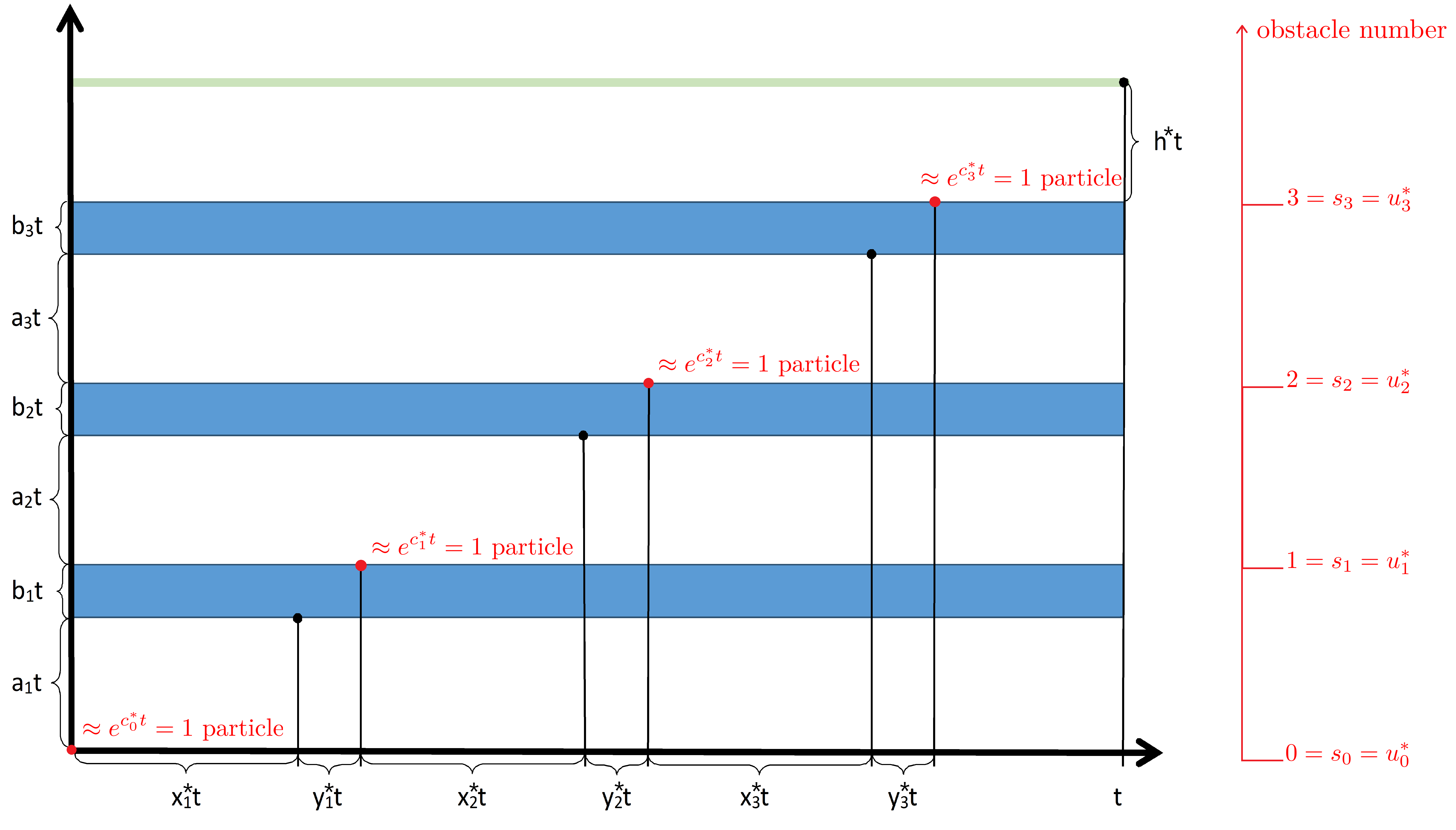
Figure 2. In our example, we have $a_{1}=a_{2}=a_{3}$ and $b_{1}=b_{2}=b_{3}$. As illustrated on the red axis, this implies $\{s_{1},\!...,s_{n}\}=\{1,2\}$ and also $0=u_{0}^{*}<1=u_{1}^{*}<2=u_{2}^{*}<3=u_{3}^{*}$. I.e. each obstacle and the corresponding branching area build a separate block. Heuristically, the optimal strategy has $\approx 1$ particle at the red dots.

3.4. Maximal particle as a descendant of one of the first particles above all obstacles

In this subsection, we show that the argmax of (3.1) over $\hat{D}$ equals the argmax of (3.1) over $D$. We start with a lemma relating the two domains to each other.

Lemma 3.21.

The domain $\hat{D}$ is not empty if and only if $D$ is not empty. Furthermore, we have

$$\sum_{i=1}^{\ell}(x_{i}^{*}+y_{i}^{*})\leq\sum_{i=1}^{\ell}(x_{i}+y_{i}),$$ (3.97)

for all $(x_{1},y_{1},\!...,x_{\ell},y_{\ell})\in D$.

Proof.

$\hat{D}$ is a subset of $D$ by definition. Conversely, for all $(x_{1},y_{1},\!...,x_{\ell},y_{\ell})\in D$ we have that

$$\left(x_{1},y_{1},\!...,x_{\ell},\frac{b_{\ell}^{2}}{2\left(\sum_{i=1}^{\ell-1}\left(x_{i}-\frac{a_{i}^{2}}{2x_{i}}-\frac{b_{i}^{2}}{2y_{i}}\right)+x_{\ell}-\frac{a_{\ell}^{2}}{2x_{\ell}}\right)}\right)\in\hat{D}.$$ (3.98)

Since the last entry of (3.98) is not greater than $y_{\ell}$, (3.97) follows by Theorem 3.14. ∎

Now, we state the main result of this section. Our candidate for the first order of the maximum of BBM among obstacles is $\sum_{i=1}^{\ell}(a_{i}+b_{i})t+h^{*}t$ where $h^{*}$ is equal to (3.99).

Theorem 3.22.

If $D$ is not empty, the maximum of (3.1) over $D$ equals $(h^{*})^{2}/2$ with

$$h^{*}=\sqrt{2}\left(1-\sum_{i=0}^{n^{*}}\left(\sum_{j=u_{i}^{*}+1}^{u_{i+1}^{*}}a_{j}f(\tilde{c}_{i})+\frac{\left(\sum_{j=u_{i}^{*}+1}^{u_{i+1}^{*}}b_{j}\right)^{2}}{2\sum_{j=u_{i}^{*}+1}^{u_{i+1}^{*}}a_{j}\left(f(\tilde{c}_{i})-\frac{1}{2f(\tilde{c}_{i})}\right)}\right)\right).$$ (3.99)

Proof.

Assume w.l.o.g. $\sum_{i=1}^{\ell}\left(x_{i}^{*}+y_{i}^{*}\right)<1$. (Otherwise $D$ and $\hat{D}$ consist of only one element.) The claim follows by Theorem 3.14 if we show

$$\left(1-\sum_{i=1}^{\ell}(x_{i}^{*}+y_{i}^{*})\right)^{2}>\left(1-\sum_{i=1}^{\ell}(x_{i}+y_{i})\right)\left(1-\sum_{i=1}^{\ell}\left(y_{i}+\frac{a_{i}^{2}}{2x_{i}}+\frac{b_{i}^{2}}{2y_{i}}\right)\right)$$ (3.100)

for all $(x_{1},y_{1},\!...,x_{\ell},y_{\ell})\in D$ that do not satisfy (3.3) with equality for $m=\ell$. If some $(x_{1},y_{1},\!...,x_{\ell},y_{\ell})$ in the interior of $D$ maximized (3.1) over $D$, it would be a critical point. In particular, the derivative of (3.1) with respect to $x_{1}$ would have to satisfy

$$-\left(1-\sum_{i=1}^{\ell}\left(y_{i}+\frac{a_{i}^{2}}{2x_{i}}+\frac{b_{i}^{2}}{2y_{i}}\right)\right)+\left(1-\sum_{i=1}^{\ell}(x_{i}+y_{i})\right)\dfrac{a_{1}^{2}}{2x_{1}^{2}}=0.$$ (3.101)

Plugging (3.101) into (3.100), it remains to show

$$\left(1-\sum_{i=1}^{\ell}(x_{i}^{*}+y_{i}^{*})\right)^{2}>\left(1-\sum_{i=1}^{\ell}(x_{i}+y_{i})\right)^{2}\dfrac{a_{1}^{2}}{2x_{1}^{2}}.$$ (3.102)

By (3.3) and $y_{1}>0$, we have $x_{1}>a_{1}/\sqrt{2}$, which implies $a_{1}^{2}/(2x_{1}^{2})<1$. Furthermore, we have $1-\sum_{i=1}^{\ell}(x_{i}^{*}+y_{i}^{*})\leq 1-\sum_{i=1}^{\ell}(x_{i}+y_{i})$ by (3.97). Consequently, (3.102) is indeed true.

It remains to look at the boundary of $D$. $x_{i}\to 0$ or $y_{i}\to 0$ would contradict (3.3) because $x_{1}+...+x_{\ell}\leq 1$ is not able to compensate $a_{i}^{2}/(2x_{i})\to\infty$ or $b_{i}^{2}/(2y_{i})\to\infty$. Equality in (3.4) would imply that the r.h.s of (3.100) equals $0$ whereas the l.h.s is assumed to be strictly positive. If (3.3) holds with equality for some $\tilde{m}<\ell$, we have to show

$$\left(1-\sum_{i=1}^{\ell}(x_{i}^{*}+y_{i}^{*})\right)^{2}>\\ \left(1-\sum_{i=1}^{\ell}(x_{i}+y_{i})\right)\left(\sum_{i=\tilde{m}+1}^{\ell}\left(x_{i}-\frac{a_{i}^{2}}{2x_{i}}-\frac{b_{i}^{2}}{2y_{i}}\right)+1-\sum_{i=1}^{\ell}(x_{i}+y_{i})\right).$$ (3.103)

If one wants to maximize the r.h.s. of (3.103) for given $(x_{1},y_{1},\!...,x_{\tilde{m}},y_{\tilde{m}})$, one can argue as above: If an interior solution was optimal, it would have to be a critical point and satisfy the first order condition with respect to $x_{\tilde{m}+1}$, which is given by

$$\left(\sum_{i=\tilde{m}+1}^{\ell}\left(x_{i}-\frac{a_{i}^{2}}{2x_{i}}-\frac{b_{i}^{2}}{2y_{i}}\right)+1-\sum_{i=1}^{\ell}(x_{i}+y_{i})\right)=\left(1-\sum_{i=1}^{\ell}(x_{i}+y_{i})\right)\frac{a_{\tilde{m}+1}^{2}}{2x_{\tilde{m}+1}^{2}}.$$ (3.104)

Plugging (3.104) into (3.103), we have to show

$$\left(1-\sum_{i=1}^{\ell}(x_{i}^{*}+y_{i}^{*})\right)^{2}>\left(1-\sum_{i=1}^{\ell}(x_{i}+y_{i})\right)^{2}\frac{a_{\tilde{m}+1}^{2}}{2x_{\tilde{m}+1}^{2}}.$$ (3.105)

This is true as $x_{\tilde{m}+1}>a_{\tilde{m}+1}/\sqrt{2}$, by (3.3) for $m=\tilde{m}+1$ and the choice of $\tilde{m}$, and $1-\sum_{i=1}^{\ell}(x_{i}^{*}+y_{i}^{*})\geq 1-\sum_{i=1}^{\ell}(x_{i}+y_{i})$ by (3.97). Hence, to show (3.100), we only have to consider those elements with equality in (3.3) for some $m>\tilde{m}$. Iterating this argument, one gets (3.100) for all elements in $D$ that do not satisfy (3.3) with equality for $m=\ell$. ∎

4. Proof of Theorem 1.4

4.1. Upper bound

We prove that, as $t\to\infty$, there exists almost surely no particle above $\sum_{i=1}^{\ell}(a_{i}+b_{i})t+(h^{*}+\epsilon)t$ (indicated by the horizontal red line in Figure 3) at time $t$.

Proposition 4.1.

Let $(a_{i},b_{i})_{i=1}^{\ell}$ be some obstacle landscape such that $\sum_{i=1}^{\ell}(x_{i}^{*}+y_{i}^{*})\leq 1$. Then, for any $\epsilon>0$, we have, almost surely,

$$\lim\limits_{t\to\infty}\frac{\max_{k\leq n(t)}X_{k}(t)}{t}<\sum_{i=1}^{\ell}(a_{i}+b_{i})+h^{*}+\epsilon.$$ (4.1)

Proof.

We show that for all $\epsilon>0$, there exists some constant $C_{2}>0$ such that

$$\mathbb{P}\left(\exists k\leq n(t):X_{k}(t)\geq\left(\sum_{i=1}^{\ell}(a_{i}+b_{i})+h^{*}+\epsilon\right)t\right)\lesssim e^{-C_{2}t}.$$ (4.2)

Since the r.h.s of (4.2) is integrable with respect to $t$, (4.1) follows by the Borel-Cantelli Lemma and approximation arguments (see e.g. [2]). We define, for $m=1,\!...,\ell$ and $k=1,\!...,n(t)$,

$$\tau_{2m-1}^{k} =\sup\left\{s\leq t:X_{k}(s)\leq\sum_{i=1}^{m-1}(a_{i}+b_{i})t+a_{m}t\right\},$$ (4.3)

$$\tau_{2m}^{k} =\inf\left\{s\geq\tau_{2m-1}^{k}:X_{k}(s)\geq\sum_{i=1}^{m}(a_{i}+b_{i})t\right\},$$ (4.4)

$$\mathcal{X}(k) =\left\{X_{k}(t)\geq\left(\sum_{i=1}^{\ell}(a_{i}+b_{i})+h^{*}+\epsilon\right)t\right\},$$ (4.5)

$$\mathcal{X}(k,n_{1},\!...,n_{2\ell}) =\mathcal{X}(k)\cap\left\{\tau_{i}^{k}\in[n_{i}-1,n_{i}]\text{ for all }i=1,\!...,2\ell\right\}.$$ (4.6)

The events $\mathcal{X}(k)$ and $\mathcal{X}(k,n_{1},\dots,n_{2l})$ are visualised in Figure 3.

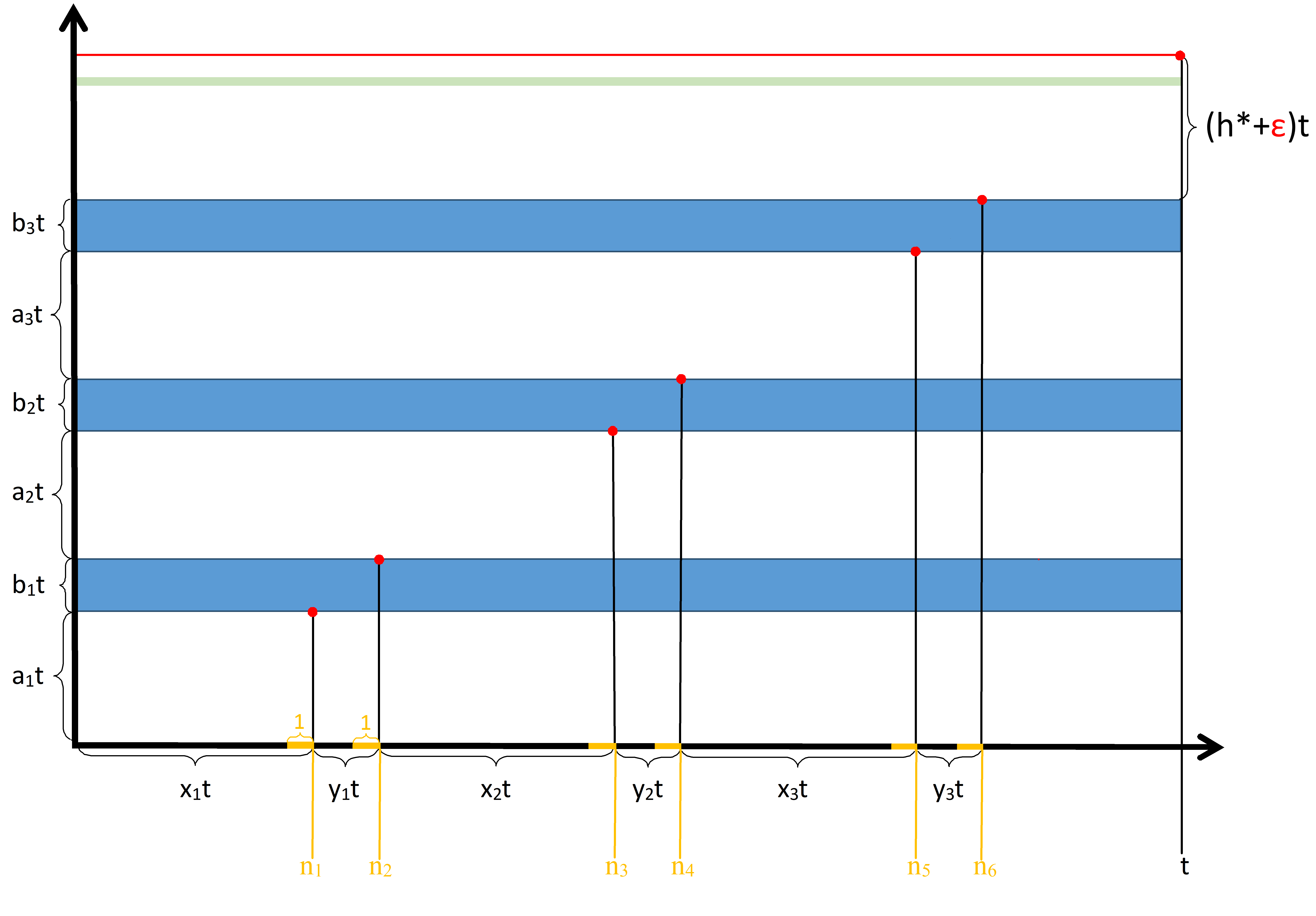
Figure 3. The horizontal red line is at height $\sum_{i=1}^{\ell}(a_{i}+b_{i})t+(h^{*}+\epsilon)t$. A particle follows the strategy marked with red dots if its last time below the $m$-th obstacle is in the interval $[n_{2m-1}-1,n_{2m-1}]$ and its next time above the $m$-th obstacle is in the interval $[n_{2m}-1,n_{2m}]$. At time $t$ it is above the horizontal red line.

The endpoints $(n_{1},\!...,n_{2\ell})$ of the intervals are in the domain

$$D_{1}=\left\{(n_{1},\!...,n_{2\ell})\in([1,t]\cap\mathbb{N})^{2\ell}:n_{1}\leq...\leq n_{2\ell}\right\}.$$ (4.7)

We rewrite the probability in (4.2) as

$$\mathbb{P}\left(\sum_{k=1}^{n(t)}\mathbbm{1}_{\mathcal{X}(k)}\geq 1\right) \leq\sum_{(n_{1},\!...,n_{2\ell})\in D_{1}}\mathbb{P}\left(\sum_{k=1}^{n(t)}\mathbbm{1}_{\mathcal{X}(k,n_{1},\!...,n_{2\ell})}\geq 1\right),$$ (4.8)

by a union bound. From now on, we set

$$(x_{1},y_{1},\!...,x_{\ell},y_{\ell})=\left(\frac{n_{1}}{t},\frac{n_{2}-n_{1}}{t},\!...,\frac{n_{2\ell-1}-n_{2\ell-2}}{t},\frac{n_{2\ell}-n_{2\ell-1}}{t}\right).$$ (4.9)

Furthermore, we define

$$D_{2}= \Big{\{}(n_{1},\!...,n_{2\ell})\in D_{1}:(x_{1},y_{1},\!...,x_{\ell},y_{\ell})\in D\Big{\}},$$ (4.10)

$$D_{3}= \Big{\{}(n_{1},\!...,n_{2\ell})\in D_{1}:(x_{1},y_{1},\!...,x_{\ell},y_{\ell})\text{ does not satisfy }\eqref{domain4}\Big{\}},$$ (4.11)

$$D_{4}= \Big{\{}(n_{1},\!...,n_{2\ell})\in D_{1}:(x_{1},y_{1},\!...,x_{\ell},y_{\ell})\text{ satisfies }\eqref{domain4}\text{ but not }\eqref{domain1}\Big{\}}.$$ (4.12)

The domain $D_{2}$ considers those elements of $D_{1}$ that correspond to the domain $D$ of the optimization problem in Section 3. The other domains are related to violating a condition of $D$. (Condition (3.4) can not be violated because of $n_{1}\leq...\leq n_{2\ell}$.) As $D_{1}=D_{2}\cup D_{3}\cup D_{4}$, (4.2) follows, once we have proven the following three lemmas.

Lemma 4.2.

Under the assumption of Proposition 4.13, there is some constant $C_{3}>0$, depending on $\epsilon$, such that

$$\sum_{(n_{1},\!...,n_{2\ell})\in D_{2}}\mathbb{P}\left(\sum_{k=1}^{n(t)}\mathbbm{1}_{\mathcal{X}(k,n_{1},\!...,n_{2\ell})}\geq 1\right)\lesssim e^{-C_{3}t}.$$ (4.13)

Lemma 4.3.

Under the assumption of Proposition 4.13, there is some constant $C_{4}>0$ such that

$$\sum_{(n_{1},\!...,n_{2\ell})\in D_{3}}\mathbb{P}\left(\sum_{k=1}^{n(t)}\mathbbm{1}_{\mathcal{X}(k,n_{1},\!...,n_{2\ell})}\geq 1\right)\lesssim e^{-C_{4}t}.$$ (4.14)

Lemma 4.4.

Under the assumption of Proposition 4.13, there is some constant $C_{5}>0$, depending on $\epsilon$, such that

$$\sum_{(n_{1},\!...,n_{2\ell})\in D_{4}}\mathbb{P}\left(\sum_{k=1}^{n(t)}\mathbbm{1}_{\mathcal{X}(k,n_{1},\!...,n_{2\ell})}\geq 1\right)\lesssim e^{-C_{5}t}.$$ (4.15)

∎

Proof of Lemma 4.2.

By Markov’s inequality, we have

$$\sum_{(n_{1},\!...,n_{2\ell})\in D_{2}}\mathbb{P}\left(\sum_{k=1}^{n(t)}\mathbbm{1}_{\mathcal{X}(k,n_{1},\!...,n_{2\ell})}\geq 1\right)\leq t^{2\ell}\max\limits_{(n_{1},\!...,n_{2\ell})\in D_{2}}\mathbb{E}\left[\sum_{k=1}^{n(t)}\mathbbm{1}_{\mathcal{X}(k,n_{1},\!...,n_{2\ell})}\right].$$ (4.16)

Next, we bound the expectation on the r.h.s. in (4.16) from above. Comparing BBM among obstacles with standard BBM and using (2.7), we get

$$\mathbb{E}\left[\sum_{k=1}^{n(x_{1}t)}\mathbbm{1}_{\left\{\tau_{1}^{k}\in[n_{1}-1,n_{1}]\right\}}\right]\lesssim\exp\left(x_{1}t-\frac{a_{1}^{2}t}{2x_{1}}\right).$$ (4.17)

Next, note that the contribution of particles with location above $a_{1}t+t^{(3/4)}$ to the expectation in (4.17) is negligible compared to the r.h.s of (4.17), as by Lemma 2.1

$$\mathbb{E}\left[\sum_{k=1}^{n(x_{1}t)}\mathbbm{1}_{\left\{\tau_{1}^{k}\in[n_{1}-1,n_{1}]\right\}\cap\left\{X_{k}(x_{1}t)>a_{1}t+t^{\frac{3}{4}}\right\}}\right]\lesssim\exp\left(x_{1}t-\frac{a_{1}^{2}t}{2x_{1}}-\frac{t^{\frac{3}{2}}}{2}\right).$$ (4.18)

Hence, we bound the way to the next branching area from below by $b_{1}t-t^{(3/4)}$ and the available time from above by $y_{1}t$. Between $\tau_{1}^{k}$ and $\tau_{2}^{k}$, $X_{k}$ does not branch. Possible branching in the small interval $[\tau_{2}^{k},n_{2}]$ can be taken into the error term. Then we get, by Lemma 2.1,

$$\mathbb{E}\left[\sum_{k=1}^{n\left((x_{1}+y_{1})t\right)}\mathbbm{1}_{\left\{\tau_{1}^{k}\in[n_{1}-1,n_{1}]\right\}\cap\left\{\tau_{2}^{k}\in[n_{2}-1,n_{2}]\right\}}\right]\lesssim\exp\left(x_{1}t-\frac{a_{1}^{2}t}{2x_{1}}-\frac{b_{1}^{2}t}{2y_{1}}\right).$$ (4.19)

Again, only particles in $[(a_{1}+b_{1})t,(a_{1}+b_{1})t+t^{(3/4)}]$ are relevant. Iterating this procedure, we obtain the upper bound

$$\mathbb{E}\left[\sum_{k=1}^{n(t)}\mathbbm{1}_{\mathcal{X}(k,n_{1},\!...,n_{2\ell})}\right]$$

$$\lesssim\exp\Bigg{(}\Bigg{[}\sum_{i=1}^{\ell}\left(x_{i}-\frac{a_{i}^{2}}{2x_{i}}-\frac{b_{i}^{2}}{2y_{i}}\right)+\left(1-\sum_{i=1}^{\ell}(x_{i}+y_{i})\right)-\frac{\left(h^{*}+\epsilon\right)^{2}}{2\left(1-\sum_{i=1}^{\ell}(x_{i}+y_{i})\right)}\Bigg{]}t\Bigg{)}$$

$$\equiv M\left(x_{1},y_{1},\!...,x_{\ell},y_{\ell}\right).$$ (4.20)

Hence, the r.h.s. of (4.16) is bounded from above by

$$\lesssim\max\limits_{(x_{1},y_{1},\!...,x_{\ell},y_{\ell})\in D}M\left(x_{1},y_{1},\!...,x_{\ell},y_{\ell}\right).$$ (4.21)

By Theorem 3.22 and simple algebraic manipulations, (4.21) can be bounded from above by

$$\exp\left(\left[\sum_{i=1}^{\ell}\left(x_{i}^{*}-\frac{a_{i}^{2}}{2x_{i}^{*}}-\frac{b_{i}^{2}}{2y_{i}^{*}}\right)+1-\sum_{i=1}^{\ell}(x_{i}^{*}+y_{i}^{*})-\frac{(h^{*}+\epsilon)^{2}}{2\left(1-\sum_{i=1}^{\ell}(x_{i}^{*}+y_{i}^{*})\right)}\right]t\right).$$ (4.22)

The exponent in (4.22) is strictly negative, because

$$2\left(1-\sum_{i=1}^{\ell}(x_{i}^{*}+y_{i}^{*})\right)\left(\sum_{i=1}^{\ell}\left(x_{i}^{*}-\frac{a_{i}^{2}}{2x_{i}^{*}}-\frac{b_{i}^{2}}{2y_{i}^{*}}\right)+1-\sum_{i=1}^{\ell}(x_{i}^{*}+y_{i}^{*})\right)$$ (4.23)

equals $(h^{*})^{2}$ which is strictly smaller than $(h^{*}+\epsilon)^{2}$. ∎

Proof of Lemma 4.3.

If $(n_{1},\!...,n_{2\ell})\in D_{3}$, we have $n_{i}=n_{i+1}$ for some $i\in\{1,\!...,2\ell\}$. In particular, a whole obstacle or branching area has to be crossed during the time interval $[n_{i}-1,n_{i}]$. For large $t$, the size of this obstacle respectively branching area is bounded from below by $t^{3/4}$. The expected number of particles at time $n_{i}$ is bounded from above by $e^{t}$. Hence, by Markov’s inequality and Lemma 2.1, we bound the l.h.s. in (4.14) from above by

$$t^{2\ell}\max\limits_{(n_{1},\!...,n_{2\ell})\in D_{3}}\mathbb{P}\left(\sum_{k=1}^{n(t)}\mathbbm{1}_{\mathcal{X}(k,n_{1},\!...,n_{2\ell})}\geq 1\right) \lesssim\exp\left(t-\frac{t^{\frac{3}{2}}}{2}\right),$$ (4.24)

which is smaller than $e^{-t}$ for large enough $t$. ∎

Proof of Lemma 4.4.

For $(n_{1},\dots,n_{2l})$ given, let $m_{1}$ be the first index such that (3.3) does not hold. Moreover, we define $m_{j}$ through

$$\sum_{i=m_{j-1}+1}^{m_{j}}\left(x_{i}-\frac{a_{i}^{2}}{2x_{i}}-\frac{b_{i}^{2}}{2y_{i}}\right)<0\quad\text{and}$$

$$\sum_{i=m_{j-1}+1}^{m}\left(x_{i}-\frac{a_{i}^{2}}{2x_{i}}-\frac{b_{i}^{2}}{2y_{i}}\right)\geq 0\text{ for all }m=m_{j-1}+1,\!...,m_{j}-1.$$ (4.25)

For notational convenience, we keep the dependence of $m_{j}$ on $(n_{1},\dots,n_{2l})$ implicit. Next, we define $D_{4}(\delta,+)$ and $D_{4}(\delta,-)$ through

$$D_{4}(\delta,+) =\left\{(n_{1},\dots,n_{2l})\in D_{4}:\exists m_{j}:\sum_{i=m_{j-1}+1}^{m_{j}}\left(x_{i}-\frac{a_{i}^{2}}{2x_{i}}-\frac{b_{i}^{2}}{2y_{i}}\right)<-\delta\right\},$$

$$D_{4}(\delta,-) =D_{4}\setminus D_{4}(\delta,+).$$ (4.26)

For $(n_{1},\dots,n_{2l})\in D_{4}(\delta,+)$ we have, by Markov’s inequality,

$$\sum_{(n_{1},\!...,n_{2\ell})\in D_{4}(\delta,+)}\mathbb{P}\left(\sum_{k=1}^{n(t)}\mathbbm{1}_{\mathcal{X}(k,n_{1},\!...,n_{2\ell})}\geq 1\right)\lesssim\exp\left(-\delta t\right).$$ (4.27)

Let $\overline{D_{4}(\delta,-)}$ be the closure of $D_{4}(\delta,-)$ and let $(\overline{x}_{1},\overline{y}_{1},\!...,\overline{x}_{\ell},\overline{y}_{\ell})$ maximize

$$\sum_{i=1}^{\ell}\left(x_{i}-\frac{a_{i}^{2}}{2x_{i}}-\frac{b_{i}^{2}}{2y_{i}}\right)+1-\sum_{i=1}^{\ell}(x_{i}+y_{i})-\frac{(h^{*}+\epsilon)^{2}}{2\left(1-\sum_{i=1}^{\ell}(x_{i}+y_{i})\right)}$$ (4.28)

over $\overline{D_{4}(\delta,-)}$. Then we have, by Markov’s inequality,

$$\sum_{(n_{1},\!...,n_{2\ell})\in\overline{D_{4}(\delta,-)}}\mathbb{P}\left(\sum_{k=1}^{n(t)}\mathbbm{1}_{\mathcal{X}(k,n_{1},\!...,n_{2\ell})}\geq 1\right)\lesssim\\ \exp\Bigg{[}\Bigg{(}\sum_{i=1}^{\ell}\left(\overline{x}_{i}-\frac{a_{i}^{2}}{2\overline{x}_{i}}-\frac{b_{i}^{2}}{2\overline{y}_{i}}\right)+1-\sum_{i=1}^{\ell}(\overline{x}_{i}+\overline{y}_{i})-\frac{(h^{*}+\epsilon)^{2}}{2\left(1-\sum_{i=1}^{\ell}(\overline{x}_{i}+\overline{y}_{i})\right)}\Bigg{)}t\Bigg{]}.$$ (4.29)

By Theorem 3.22 and simple computations, the maximum of (4.28) over $D$ is attained at $(x_{1}^{*},y_{1}^{*},\!...,x_{\ell}^{*},y_{\ell}^{*})$ and strictly negative. Since $\lim\limits_{\delta\searrow 0}\overline{D_{4}(\delta,-)}\left(\hat{\delta}\right)\subset D_{2}$, we can choose $\delta>0$ so small that the exponent on the r.h.s. of (4.29) is also strictly negative. Combining (4.27) and (4.29), we get (4.15) via a union bound, by choosing $\delta>0$ small enough. ∎

4.2. Lower bound

In this subsection, we prove the following proposition.

Proposition 4.5.

Let $(a_{i},b_{i})_{i=1}^{\ell}$ be some obstacle landscape such that $\sum_{i=1}^{\ell}(x_{i}^{*}+y_{i}^{*})\leq 1$. Then, for any $\epsilon>0$, we have, almost surely,

$$\lim\limits_{t\to\infty}\frac{\max_{k\leq n(t)}X_{k}(t)}{t}>\sum_{i=1}^{\ell}(a_{i}+b_{i})+h^{*}-\epsilon.$$ (4.30)

Before proving Proposition 4.5, we need to introduce some notation. For $\delta>0$ and $C>0$, we define, for $m=1,\!...,\ell$, the intervals

$$I_{m}^{A} =\sum_{i=1}^{m-1}(a_{i}+b_{i})t+\left[(a_{m}-\delta)t,a_{m}t\right],\quad I_{m}^{B}=\sum_{i=1}^{m}(a_{i}+b_{i})t+\left[\delta t,\delta t+C\right].$$ (4.31)

Moreover, we define, for $k\leq n(t)$, the events

$$A_{m}^{k} =\left\{X_{k}\left(\sum_{i=1}^{m-1}(x_{i}^{*}+y_{i}^{*})t+x_{m}^{*}t+\hat{\delta}t\right)\in I_{m}^{A}\right\},$$ (4.32)

$$B_{m}^{k} =\left\{X_{k}\left(\sum_{i=1}^{m}(x_{i}^{*}+y_{i}^{*})t+\hat{\delta}t\right)\in I_{m}^{B}\right\}.$$ (4.33)

To prove Proposition 4.5, we show that there is a particle $X_{k}$ such that $X_{k}\in\bigcap_{m=1}^{\ell}\left(A_{m}^{k}\cap B_{m}^{k}\right)$ and $X_{k}(t)/t$ is larger than the r.h.s. of (4.30).

Proof.

First, assume $\sum_{i=1}^{\ell}(x_{i}^{*}+y_{i}^{*})<1$ and let w.l.o.g. $\epsilon/\sqrt{2}\in(0,1-\sum_{i=1}^{\ell}(x_{i}^{*}+y_{i}^{*}))$. We fix the additional time $\hat{\delta}>0$ such that $\hat{\delta}<\epsilon/\sqrt{2}$.

We introduce some events, see Figure 4 for an illustration.

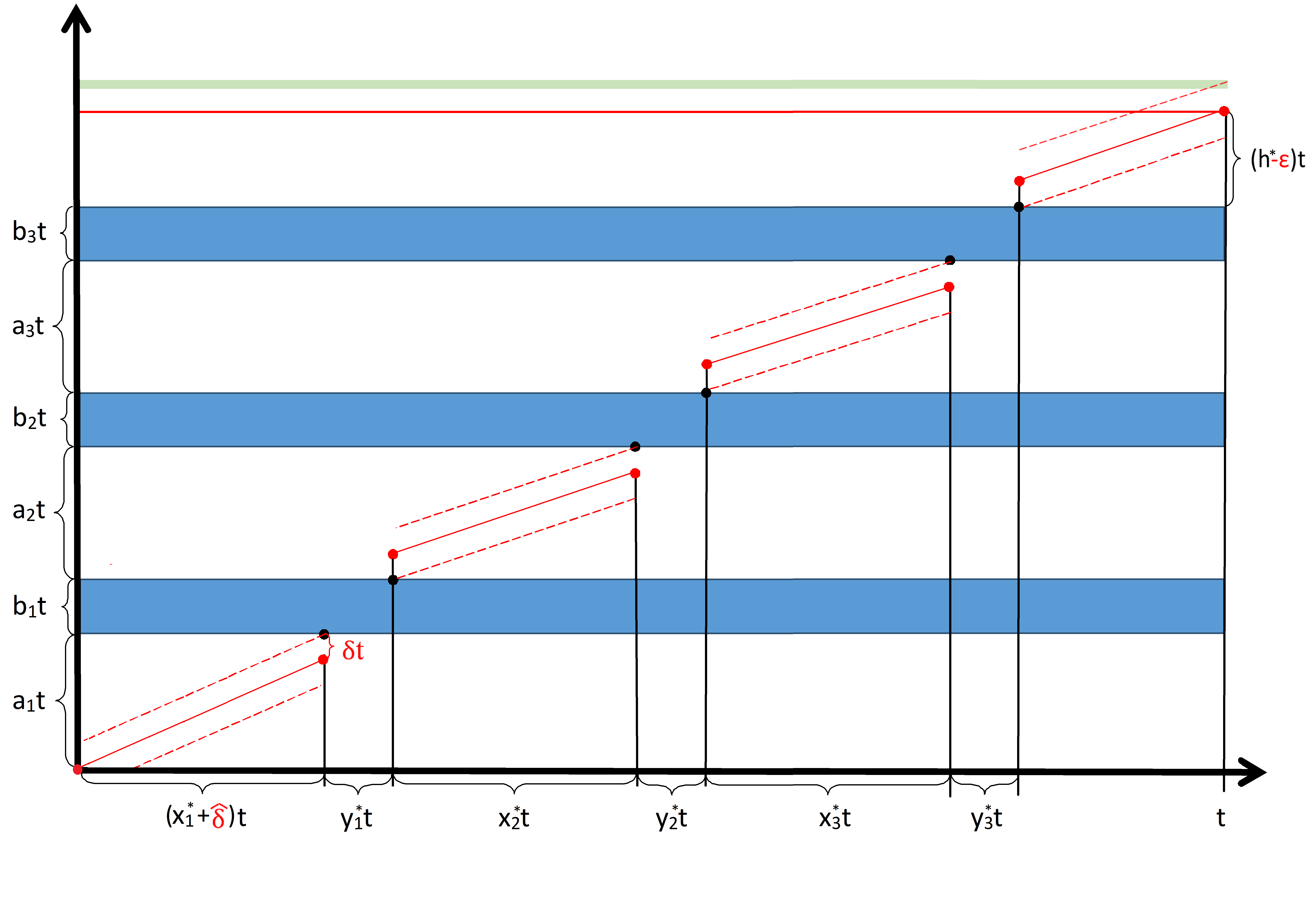
Figure 4. The horizontal red line is at height $\sum_{i=1}^{\ell}(a_{i}+b_{i})t+(h^{*}-\epsilon)t$. To prove Proposition 4.5, we show that a certain number of particles follows the strategy marked with red dots.

We define, for $m=1,\!...,\ell$ and some constant $C>0$,

$$\mathcal{A}_{m} =\left\{\exists t_{0}\forall t>t_{0}:\#\left\{k\leq n\left(\sum_{i=1}^{m-1}(x_{i}^{*}+y_{i}^{*})t+x_{m}^{*}t+\hat{\delta}t\right):A_{m}^{k}\right\}\geq e^{\alpha_{m}t}\right\},$$ (4.34)

$$\mathcal{B}_{m} =\left\{\exists t_{0}\forall t>t_{0}:\#\left\{k\leq n\left(\sum_{i=1}^{m}(x_{i}^{*}+y_{i}^{*})t+\hat{\delta}t\right):B_{m}^{k}\right\}\geq e^{\beta_{m}t}\right\},$$ (4.35)

where

$$\alpha_{m} =\sum_{i=1}^{m}\left(x_{i}^{*}+\hat{\delta}\mathbbm{1}_{i=1}-\frac{(a_{i}-\delta)^{2}}{2(x_{i}^{*}+\hat{\delta}\mathbbm{1}_{i=1})}-\frac{(b_{i}+2\delta)^{2}}{2y_{i}^{*}}\right)+\frac{(b_{m}+2\delta)^{2}}{2y_{m}^{*}}-(2m-1)\gamma,$$ (4.36)

$$\beta_{m} =\alpha_{m}-\frac{(b_{m}+2\delta)^{2}}{2y_{m}^{*}}-\gamma.$$ (4.37)

Moreover, we define

$$\mathcal{H}=\left\{\exists t_{0}\forall t>t_{0}\exists k\leq n(t):X_{k}(t)\geq\left(\sum_{i=1}^{\ell}(a_{i}+b_{i})+h^{*}-\epsilon\right)t\right\}.$$ (4.38)

Since $(x_{1}^{*},y_{1}^{*},\!...,x_{\ell}^{*},y_{\ell}^{*})$ is in $D$, we have

$$\sum_{i=1}^{m}\left(x_{i}^{*}-\frac{a_{i}^{2}}{2x_{i}^{*}}-\frac{b_{i}^{2}}{2y_{i}^{*}}\right)\geq 0\mbox{ and }\sum_{i=1}^{m-1}\left(x_{i}^{*}-\frac{a_{i}^{2}}{2x_{i}^{*}}-\frac{b_{i}^{2}}{2y_{i}^{*}}\right)+x_{m}^{*}-\frac{a_{m}^{2}}{2x_{m}^{*}}\geq 0$$ (4.39)

for all $m=1,\!...,\ell$ . If we replace $x_{1}^{*}t$ by $(x_{1}^{*}+\hat{\delta})t$, the inequalities in (4.39) are strict. By continuity, we can choose the tube width parameter $\delta>0$ and the error parameter $\gamma>0$ so small, depending on $\hat{\delta}$, that $\alpha_{m}>0$ and $\beta_{m}>0$ for all $m=1,\!...,\ell$. The probability of $\mathcal{H}$ should go to one. By monotonicity and the Markov property, we have the lower bound

$$\mathbb{P}\left(\mathcal{H}\right)\geq \mathbb{P}\left(\bigcap_{m=1}^{\ell}\left(\mathcal{A}_{m}\cap\mathcal{B}_{m}\right)\cap\mathcal{H}\right)$$ (4.40)

$$= \mathbb{P}\left(\mathcal{H}\middle|\mathcal{B}_{\ell}\right)\left(\prod_{m=2}^{\ell}\mathbb{P}\left(\mathcal{B}_{m}\middle|\mathcal{A}_{m}\right)\mathbb{P}\left(\mathcal{A}_{m}\middle|\mathcal{B}_{m-1}\right)\right)\mathbb{P}\left(\mathcal{B}_{1}\middle|\mathcal{A}_{1}\right)\mathbb{P}\left(\mathcal{A}_{1}\right).$$ (4.41)

By Lemmas 4.6, 4.7, 4.8 and 2.2, each factor of (4.41) is equal to one. The claim (4.30) follows.

If $\sum_{i=1}^{\ell}(x_{i}^{*}+y_{i}^{*})=1$, one could choose $\hat{\delta}>0$ so small that the inequalities in (4.39) with $b_{\ell}$ replaced by $b_{\ell}-\epsilon$, $x_{1}^{*}$ replaced by $x_{1}^{*}+\hat{\delta}$ and $y_{\ell}^{*}$ replaced by $y_{\ell}^{*}-\hat{\delta}$ are strict. Then one could define $\alpha_{m}$, $\beta_{m}$, $A_{m}^{k}$, $B_{m}^{k}$, $\mathcal{A}_{m}$ and $\mathcal{B}_{m}$ as above but with $b_{\ell}+2\delta$ replaced by $b_{\ell}+\delta-\epsilon$ and $y_{m}^{*}$ replaced by $y_{m}^{*}-\hat{\delta}$. One could choose $\delta>0$ and $\gamma>0$ so small that $\alpha_{m}$ and $\beta_{m}$ are strictly positive. In (4.40), one would have $\mathbb{P}\left(\mathcal{H}\middle|\mathcal{B}_{\ell}\right)=1$ by $\mathcal{B}_{\ell}\subset\mathcal{H}$. The remaining computations would work analogously. ∎

Lemma 4.6.

Under the assumption of Proposition 4.5 and for $\sum_{i=1}^{\ell}(x_{i}^{*}+y_{i}^{*})<1$, we have $\mathbb{P}\left(\mathcal{H}\middle|\mathcal{B}_{\ell}\right)=1$.

Proof.

By Lemma 2.2, we can bound $\mathbb{P}\left(\mathcal{H}\middle|\mathcal{B}_{\ell}\right)$ by considering a BBM without obstacles. We have

$$\mathbb{P}\left(\mathcal{H}\middle|\mathcal{B}_{\ell}\right)\geq\mathbb{P}\Bigg{[}\exists t_{0}\forall t>t_{0}\exists k\leq\hat{n}\left(\left(1-\sum_{i=1}^{\ell}(x_{i}^{*}+y_{i}^{*})-\hat{\delta}\right)t\right):\\ \widehat{X}_{k}\left(\left(1-\sum_{i=1}^{\ell}(x_{i}^{*}+y_{i}^{*})-\hat{\delta}\right)t\right)\geq\left(h^{*}-\epsilon-\delta\right)t\Bigg{]}.$$ (4.42)

Since we chose $\hat{\delta}<\epsilon/\sqrt{2}$, we have

$$\sqrt{2}\left(1-\sum_{i=1}^{\ell}(x_{i}^{*}+y_{i}^{*})-\hat{\delta}\right)>\sqrt{2}\left(1-\sum_{i=1}^{\ell}(x_{i}^{*}+y_{i}^{*})\right)-\epsilon-\delta.$$ (4.43)

Hence, the r.h.s of (4.42) equals one by the tightness of the maximum of homogeneous BBM around $m(t)$, see [13].

∎

Lemma 4.7.

Under the assumption of Proposition 4.5, we have $\mathbb{P}\left(\mathcal{B}_{m}\middle|\mathcal{A}_{m}\right)=1$ for $m=1,\!...,\ell$.

Proof.

We show that

$$1-\mathbb{P}\left(\#\left\{k\leq n\left(\sum_{i=1}^{m}(x_{i}^{*}+y_{i}^{*})t+\hat{\delta}t\right):B_{m}^{k}\right\}\geq e^{\beta_{m}t}\middle|\mathcal{A}_{m}\right)$$ (4.44)

is integrable with respect to $t$. This implies $\mathbb{P}\left(\mathcal{B}_{m}\middle|\mathcal{A}_{m}\right)=1$ for $m=1,\!...,\ell$ by the Borel-Cantelli Lemma and approximation arguments (see e.g. [2]).

For $i=1,\!...,e^{\alpha_{m}t}$ with w.l.o.g. $e^{\alpha_{m}t}\in\mathbb{N}$, we define some independent Gaussian random variables $Y_{i}\sim\mathcal{N}\left(0,y_{m}^{*}t\right)$. By monotonicity, we can ignore possible branching and ask how many of the Gaussian random variables are in $\tilde{I}_{m}^{B}=[(b_{m}+2\delta)t,(b_{m}+2\delta)t+C]$. I.e. we bound (4.44) from above by

$$1-\mathbb{P}\left(\sum_{i=1}^{e^{\alpha_{m}t}}\mathbbm{1}_{Y_{i}\in\tilde{I}_{m}^{B}}\geq e^{\beta_{m}+\gamma t-\gamma t}\right).$$ (4.45)

To apply the Paley-Zygmund inequality, we compute the expectation and the second moment. By Lemma 2.1, we get

$$\mathbb{E}\left[\sum_{i=1}^{e^{\alpha_{m}t}}\mathbbm{1}_{Y_{i}\in\tilde{I}_{m}^{B}}\right]\approx\exp\left({\alpha_{m}t-\frac{(b_{m}+2\delta)^{2}t}{2y_{m}^{*}}}\right)=e^{\beta_{m}+\gamma t}.$$ (4.46)

By Lemma 2.1 and the independence of $Y_{i}$, we have

$$\mathbb{E}\left[\left(\sum_{i=1}^{e^{\alpha_{m}t}}\mathbbm{1}_{Y_{i}\in\tilde{I}_{m}^{B}}\right)^{2}\right]=\mathbb{E}\left[\sum_{i=1}^{e^{\alpha_{m}t}}\sum_{j=1}^{e^{\alpha_{m}t}}\mathbbm{1}_{Y_{i}\in\tilde{I}_{m}^{B}}\mathbbm{1}_{Y_{j}\in\tilde{I}_{m}^{B}}\right]$$ (4.47)

$$\approx e^{\beta_{m}+\gamma t}+e^{2(\beta_{m}+\gamma t)}-\exp\left({\alpha_{m}t-2\frac{(b_{m}+2\delta)^{2}t}{2y_{m}^{*}}}\right),$$ (4.48)

where the first summand of (4.48) considers the diagonal and the second and third summands consider all the other terms. Hence, by the Paley-Zygmund inequality, we can bound (4.45) from above by

$$1-\mathbb{P}\left(\sum_{i=1}^{e^{\alpha_{m}t}}\mathbbm{1}_{Y_{i}\in\tilde{I}_{m}^{B}}\geq e^{\beta_{m}+\gamma t-\gamma t}\right)\leq 1-\left(1-e^{-\gamma t}\right)^{2}\frac{e^{2(\beta_{m}+\gamma)t}}{e^{(\beta_{m}+\gamma)t}+e^{2(\beta_{m}+\gamma)t}}.$$ (4.49)

Let $C_{6}>0$. The r.h.s of (4.49) is smaller than $e^{-C_{6}t}$ if and only if

$$1-e^{-C_{6}t}+e^{-(\beta_{m}+\gamma)t}-e^{-(\beta_{m}+\gamma+C_{6})t}<1+e^{-2\gamma t}-2e^{-\gamma t}.$$ (4.50)

By definition of $\beta_{m}>0$, we can choose $\gamma>0$ so small that still $\beta_{m}>0$ but also $\beta_{m}+\gamma>2\gamma$ for all $m=1,\!...,\ell-1$. Afterwards, we choose $C_{6}>0$ such that $C_{6}<\gamma$. Then (4.50) is indeed true and we can bound (4.44) from above by $e^{-C_{6}t}$. ∎

Lemma 4.8.

Under the assumption of Proposition 4.5, we have $\mathbb{P}\left(\mathcal{A}_{m}\middle|\mathcal{B}_{m-1}\right)=1$ for $m=2,\!...,\ell$.

Proof.

This proof is similar to the one of Lemma 4.7. We want to show that

$$1-\mathbb{P}\left(\#\left\{k\leq n\left(\sum_{i=1}^{m-1}(x_{i}^{*}+y_{i}^{*})t+x_{m}^{*}t+\hat{\delta}t\right):A_{m}^{k}\right\}\geq e^{\alpha_{m}t}\middle|\mathcal{B}_{m-1}\right)$$ (4.51)

is integrable with respect to $t$. This implies $\mathbb{P}\left(\mathcal{A}_{m}\middle|\mathcal{B}_{m-1}\right)=1$ for $m=2,\!...,\ell$ by the Borel-Cantelli Lemma and approximation arguments (see e.g. [2]).

We look at $e^{\beta_{m-1}t}$ independent BBMs that start in $0$ without obstacles. Denote by $\mathcal{Y}_{i}$ the event that the $i$-th BBM has at least $\exp(x_{m}^{*}t-(a_{m}-\delta)^{2}t/(2x_{m}^{*})-\gamma t/3)$ particles in $[(a_{m}-\delta)t,a_{m}t]$ at time $x_{m}^{*}t$. By Lemma 2.2, we can bound (4.51) from above by

$$1-\mathbb{P}\left(\sum_{i=1}^{e^{\beta_{m-1}t}}\mathbbm{1}_{\mathcal{Y}_{i}}\geq e^{(\beta_{m-1}-2\gamma/3)t}\right).$$ (4.52)

Since, by Lemma 2.2, $\mathbb{P}(\mathcal{Y}_{i})\to 1$, as $t\to\infty$, it can be bounded from below by $\exp(-\gamma t/3)$ for large enough $t$. Analogously to (4.49), we can bound the probability in (4.52) from below by

$$\mathbb{P}\left(\sum_{i=1}^{e^{\beta_{m-1}t}}\mathbbm{1}_{\mathcal{Y}_{i}}\geq\mathbb{P}\left(\mathcal{Y}_{i}\right)e^{(\beta_{m-1}-\gamma/3)t}\right) \geq\left(1-e^{-\gamma t/3}\right)^{2}\frac{e^{2\beta_{m-1}t}\mathbb{P}\left(\mathcal{Y}_{i}\right)^{2}}{e^{\beta_{m-1}t}\mathbb{P}\left(\mathcal{Y}_{i}\right)+e^{2\beta_{m-1}t}\mathbb{P}\left(\mathcal{Y}_{i}\right)^{2}},$$ (4.53)

using Paley-Zygmunds inequality and the independence of the BBMs. Let $C_{7}>0$. The expression (4.53) is smaller than $e^{-C_{7}t}$ if and only if

$$e^{-\beta_{m-1}t}-e^{-(C_{7}+\beta_{m-1})t}-e^{-C_{7}t}\mathbb{P}(\mathcal{Y}_{i})\leq e^{-\frac{2}{3}\gamma t}\mathbb{P}(\mathcal{Y}_{i})-2e^{-\frac{\gamma}{3}t}\mathbb{P}(\mathcal{Y}_{i}).$$ (4.54)

By definition of $\beta_{m-1}>0$, we can choose $\gamma>0$ so small that still $\beta_{m-1}>0$ but also $2\gamma/3<\beta_{m-1}$ for all $m=2,\!...,\ell$. Afterwards, we choose $C_{7}>0$ such that $C_{7}<\gamma/3$. Then (4.54) is indeed true and we can bound (4.51) from above by $e^{-C_{7}t}$. ∎

Appendix A Differentiability of $x_{m}^{c}$

In this appendix, we show differentiability of $x_{m}^{c}$ with respect to $c_{m}$. Differentiability of $x_{m}^{c}$ with respect to $c_{m-1}$ can be proved analogously. For $(c_{1},\!...,c_{\ell})\in D^{c}$, we define $\mathcal{I}(c_{m})=\{C\in\mathbb{R}:(c_{1},\!...,c_{m-1},C,c_{m+1},\!...,c_{\ell})\in D^{c}\}$. First, we show that $x_{m}(C)$ is continuous in $C$ on $\mathcal{I}(c_{m})$ and a simple root of some polynomial. Then we use the implicit function theorem to show differentiability in the interior of $\mathcal{I}(c_{m})$. We start with some auxiliary results.

Corollary A.1.

For all $(c_{1},\!...,c_{\ell})\in D^{c}$, $\mathcal{I}(c_{m})$ is an interval.

Proof.

The claim follows from Lemma 3.3. ∎

Lemma A.2.

For all $C\in\mathcal{I}(c_{m})$, the domain $D^{m}_{x}(c_{m-1},C)$ is a closed interval.

Proof.

Connectivity of $D^{m}_{x}(c_{m-1},C)$ can be proved analogously to the proof of Lemma 3.3. To show that $D^{m}_{x}(c_{m-1},C)$ is closed, let $x_{m}^{i}\in D^{m}_{x}(c_{m-1},C)$ be some convergent sequence. We have

$$c_{m-1}+x_{m}^{i}-\frac{a_{m}^{2}}{2x_{m}^{i}}-\frac{b_{m}^{2}}{2y_{m}^{i}}=C,$$ (A.1)

$$x_{m}^{i}+y_{m}^{i}\leq N,$$ (A.2)

$$x_{m}^{i}>0\text{ and }y_{m}^{i}>0$$ (A.3)

with

$$y_{m}^{i}=\frac{b_{m}^{2}}{2\left(c_{m-1}-C+x_{m}^{i}-\frac{a_{m}^{2}}{2x_{m}^{i}}\right)}.$$ (A.4)

Let $\hat{x}=\lim\limits_{i\to\infty}x_{m}^{i}$. By (A.1), it is not possible that $\hat{x}=0$ because $x_{m}^{i}\leq N$ is not able to compensate $a_{m}^{2}/(2x_{m}^{i})\to\infty$. Furthermore, the denominator of (A.4) can not converge to $0$ because $y_{m}^{i}\leq N$. Hence, $\hat{y}=\lim\limits_{i\to\infty}y_{m}^{i}$ is well defined. We have to show

$$c_{m-1}+\hat{x}-\frac{a_{m}^{2}}{2\hat{x}}-\frac{b_{m}^{2}}{2\hat{y}}=C,$$ (A.5)

$$\hat{x}+\hat{y}\leq N,$$ (A.6)

$$\hat{x}>0\text{ and }\hat{y}>0.$$ (A.7)

By (A.1), it is also not possible that $\hat{y}=0$ because $x_{m}^{i}\leq N$ is not able to compensate $b_{m}^{2}/(2y_{m}^{i})\to\infty$. Hence, (A.7) holds. The conditions (A.5) and (A.6) follow from (A.1) and (A.2) by continuity. Hence, $\hat{x}\in D^{m}_{x}(c_{m-1},C)$ and $D^{m}_{x}(c_{m-1},C)$ is closed. ∎

Lemma A.3.

For all $\hat{C}\in\mathcal{I}(c_{m})$, all $\hat{x}\in D^{m}_{x}(c_{m-1},\hat{C})$ and all $\epsilon>0$ such that $\{x\in\mathbb{R}:|x-\hat{x}|<2\epsilon\}\subset D^{m}_{x}(c_{m-1},\hat{C})$, there exists $\delta>0$ such that for all $C\in\mathcal{I}(c_{m})$ with $|C-\hat{C}|<\delta$ we have $\{x\in\mathbb{R}:|x-\hat{x}|<\epsilon\}\subset D^{m}_{x}(c_{m-1},C)$.

Proof.

Since $D^{m}_{x}(c_{m-1},\hat{C})$ is closed by Lemma A.2, we have $\{x\in\mathbb{R}:|x-\hat{x}|\leq 2\epsilon\}\subset D^{m}_{x}(c_{m-1},\hat{C})$. Hence, we have for all $\alpha\in[-2,2]$,

$$c_{m-1}+\hat{x}+\epsilon\alpha-\frac{a_{m}^{2}}{2(\hat{x}+\epsilon\alpha)}-\frac{b_{m}^{2}}{2y(\alpha)}=\hat{C},$$ (A.8)

$$\hat{x}+\epsilon\alpha+y(\alpha)\leq N,$$ (A.9)

$$\hat{x}+\epsilon\alpha>0\text{ and }y(\alpha)>0$$ (A.10)

with

$$y(\alpha)=\frac{b_{m}^{2}}{2\left(c_{m-1}-\hat{C}+\hat{x}+\epsilon\alpha-\frac{a_{m}^{2}}{2(\hat{x}+\epsilon\alpha)}\right)}.$$ (A.11)

We have to show that there is some $\delta>0$ such that for all $\beta\in(-1,1)$ and all $\alpha\in(-1,1)$,

$$c_{m-1}+\hat{x}+\epsilon\alpha-\frac{a_{m}^{2}}{2(\hat{x}+\epsilon\alpha)}-\frac{b_{m}^{2}}{2y(\alpha,\beta)}=\hat{C}+\delta\beta,$$ (A.12)

$$\hat{x}+\epsilon\alpha+y(\alpha,\beta)\leq N,$$ (A.13)

$$\hat{x}+\epsilon\alpha>0\text{ and }y(\alpha,\beta)>0$$ (A.14)

with

$$y(\alpha,\beta)=\frac{b_{m}^{2}}{2\left(c_{m-1}-\hat{C}-\delta\beta+\hat{x}+\epsilon\alpha-\frac{a_{m}^{2}}{2(\hat{x}+\epsilon\alpha)}\right)}.$$ (A.15)

For $\alpha\in[-2,2]$, we define $F_{0}(\alpha)=2\left(c_{m-1}-\hat{C}+\hat{x}+\epsilon\alpha-\frac{a_{m}^{2}}{2(\hat{x}+\epsilon\alpha)}\right)$ and $\alpha^{0}=\text{argmin}\{F_{0}(\alpha):\alpha\in[-2,2]\}$. Note that $\alpha^{0}$ is well defined because $F_{0}$ is strictly concave on $[-2,2]$ by (A.10). By (A.10) and (A.11), we have $F_{0}(\alpha^{0})>0$. Let $\hat{\delta}>0$ be so small that also $F_{0}(\alpha^{0})-2\hat{\delta}>0$. Then we have

$$\frac{b_{m}^{2}}{2\left(c_{m-1}-\hat{C}-\hat{\delta}\beta+\hat{x}+\epsilon\alpha-\frac{a_{m}^{2}}{2(\hat{x}+\epsilon\alpha)}\right)}\geq\frac{b_{m}^{2}}{F_{0}(\alpha^{0})-2\hat{\delta}}>0$$ (A.16)

for all $\beta\in[-1,1]$ and all $\alpha\in[-2,2]$.

For $\delta\in(0,\hat{\delta})$ and $\alpha\in[-2,2]$, we define

$$F_{1}(\delta,\alpha)=\hat{x}+\epsilon\alpha+\frac{b_{m}^{2}}{2\left(c_{m-1}-\hat{C}-\delta+\hat{x}+\epsilon\alpha-\frac{a_{m}^{2}}{2(\hat{x}+\epsilon\alpha)}\right)}.$$ (A.17)

By (3.29) in the proof of Proposition 3.4, $F_{1}(0,\alpha)$ is strictly convex in $\alpha$ on $[-2,2]$. Hence, $\alpha^{1}=\text{argmax}\{F_{1}(0,\alpha):\alpha\in[-1,1]\}$ is well defined and satisfies $F_{1}(0,\alpha^{1})<F_{1}(0,2)\leq N$ or $F_{1}(0,\alpha^{1})<F_{1}(0,-2)\leq N$.

The derivative of $F_{1}$ with respect to $\delta$ is equal to

$$\partial_{\delta}F_{1}(\delta,\alpha)=\frac{b_{m}^{2}}{2\left(c_{m-1}-\hat{C}-\delta+\hat{x}+\epsilon\alpha-\frac{a_{m}^{2}}{2(\hat{x}+\epsilon\alpha)}\right)^{2}}.$$ (A.18)

We bound $\partial_{\delta}F_{1}(\delta,\alpha)$ from above by $L=\partial_{\delta}F_{1}(\hat{\delta},\alpha^{0})$. Then we have

$$|F_{1}(\delta,\alpha)-F_{1}(0,\alpha)|\leq L\delta.$$ (A.19)

Hence, for $\delta<\min\{\hat{\delta},(N-F_{1}(0,\alpha^{1}))/L\}$, we have

$$\hat{x}+\epsilon\alpha+y(\alpha,\beta) =\hat{x}+\epsilon\alpha+\frac{b_{m}^{2}}{2\left(c_{m-1}-\hat{C}-\delta\beta+\hat{x}+\epsilon\alpha-\frac{a_{m}^{2}}{2(\hat{x}+\epsilon\alpha)}\right)}\leq F_{1}(\delta,\alpha),$$ (A.20)

which is bounded from above by $F_{1}(\delta,\alpha)\leq F_{1}(0,\alpha)+L\delta\leq N$, for all $\beta\in(-1,1)$ and all $\alpha\in(-1,1)$. ∎

Looking at the first order condition (3.25) with $c_{m}$ replaced by $C$ is equivalent to looking at roots of the polynomial

$$x^{4}+2(c_{m-1}-C)x^{3}+\left((c_{m-1}-C)^{2}-a_{m}^{2}-\frac{b_{m}^{2}}{2}\right)x^{2}-a_{m}^{2}(c_{m-1}-C)x+\frac{a_{m}^{2}}{4}(a_{m}^{2}-b_{m}^{2}).$$ (A.21)

By Proposition 3.4, we have the following corollary.

Corollary A.4.

For all $C\in\mathcal{I}(c_{m})$, $x_{m}(C)$ is the largest real root of (A.21), the only root of (A.21) in $D^{m}_{x}(c_{m-1},C)$ and not a boundary point of $D^{m}_{x}(c_{m-1},C)$.

Lemma A.5.

The four roots of (A.21) are continuous in $C$ on $\mathbb{R}$.

Proof.

The coefficients of (A.21) are continuous in $C$ on $\mathbb{R}$. This implies continuity of the roots by [II 5.2, [27]]. ∎

Lemma A.6.

Let $p(x)=a(4)x^{4}+a(3)x^{3}+a(2)x^{2}+a(1)x^{1}+a(0)$ be some polynomial with real coefficients $a(0),a(1),a(2),a(3),a(4)$ and $a(4)\neq 0$. Let $\Delta$ be the discriminant of $p$. Assume

$$8a(4)a(2)-3a(3)^{2}<0,$$ (A.22)

$$64a(4)^{3}a(0)-16a(4)^{2}a(2)^{2}+16a(4)a(3)^{2}a(2)-16a(4)^{2}a(3)a(1)-3a(3)^{4}<0.$$ (A.23)

Furthermore, assume that $\Delta=0$ implies $a(2)^{2}-3a(3)a(1)+12a(4)a(0)\neq 0$. Then $p$ has four simple real roots if $\Delta>0$, two simple real roots and two complex roots if $\Delta<0$, and two simple real roots and one real double root if $\Delta=0$.

Proof.

The claim is a special case of [32]. ∎

Now, we use these auxiliary results to prove continuity and simplicity of $x_{m}(C)$.

Lemma A.7.

For all $(c_{1},\!...,c_{\ell})\in D^{c}$, $x_{m}(C)$ is continuous in $C$ on $\mathcal{I}(c_{m})$ and a simple root of (A.21).

Proof.

We compute

$$\Delta=\frac{1}{4}\Big{(}64a_{m}^{8}b_{m}^{4}-48a_{m}^{6}b_{m}^{6}+96a_{m}^{6}b_{m}^{4}(c_{m-1}-C)^{2}-15a_{m}^{4}b_{m}^{8}-48a_{m}^{4}b_{m}^{6}(c_{m-1}-C)^{2}\\ +48a_{m}^{4}b_{m}^{4}(c_{m-1}-C)^{4}-a_{m}^{2}b_{m}^{10}+6a_{m}^{2}b_{m}^{8}(c_{m-1}-C)^{2}-12a_{m}^{2}b_{m}^{6}(c_{m-1}-C)^{4}+8a_{m}^{2}b_{m}^{4}(c_{m-1}-C)^{6}\Big{)},$$ (A.24)

the discriminant of (A.21). Note that $\Delta$ is continuous in $C$ on $\mathbb{R}$ and there are at most six $C$ such that $\Delta=0$. Between these roots, $\Delta$ does not change its sign. By elementary algebraic manipulations and Lemma A.6, we have three cases:

$\Delta>0$	(A.21) has four simple real roots
$\Delta<0$	(A.21) has two simple real roots and two complex roots
$\Delta=0$	(A.21) has one double real root and two simple real roots

Within each connected component of $\{C\in\mathcal{I}(c_{m}):\Delta>0\}$, the four roots of (A.21) can not change their order by Lemma A.5. Since $x_{m}(C)$ is the largest one by Corollary A.4, $x_{m}(C)$ is continuous in $C$ on $\{C\in\mathcal{I}(c_{m}):\Delta>0\}$ and a simple root.

Assume there exists a sequence $C(i)$ such that $C(i)$ is in the same connected component of $\{C\in\mathcal{I}(c_{m}):\Delta>0\}$ for all $i$ and, as $i\to\infty$, we have $C(i)\to\hat{C}\in\mathcal{I}(c_{m})$ and $\Delta\searrow 0$. Then the roots of (A.21) stay real and simple, do not change their order and two of them converge to the same real number. By Corollary A.4, the root that represents $x_{m}(C(i))$ is in the interior of $D^{m}_{x}(c_{m-1},C(i))$ and the only root in $D^{m}_{x}(c_{m-1},C(i))$. By Lemmas A.2, A.3 and A.5, the limit of the root that represents $x_{m}(C(i))$ for all $i$ is in $D^{m}_{x}(c_{m-1},\hat{C})$. By Corollary A.4, there is only one root in $D^{m}_{x}(c_{m-1},\hat{C})$ and this root is not a boundary point. Hence, the double root can not be in $D^{m}_{x}(c_{m-1},\hat{C})$ and $\lim\limits_{i\to\infty}x_{m}(C(i))=x_{m}(\hat{C})$ is a simple root.

Within each connected component of $\{C\in\mathcal{I}(c_{m}):\Delta<0\}$, the two real roots of (A.21) can not change their order or become non real by Lemma A.5. Since $x_{m}(C)$ is the larger one by Corollary A.4, $x_{m}(C)$ is continuous in $C$ on $\{C\in\mathcal{I}(c_{m}):\Delta<0\}$ and a simple root.

Assume there exists a sequence $C(i)$ such that $C(i)$ is in the same connected component of $\{C\in\mathcal{I}(c_{m}):\Delta<0\}$ for all $i$ and, as $i\to\infty$, we have $C(i)\to\hat{C}\in\mathcal{I}(c_{m})$ and $\Delta\nearrow 0$. Then the two complex roots become a real double root and the other roots stay simple and real. As in the case of $\Delta\searrow 0$, the limit of the root that represents $x_{m}(C(i))$ for all $i$ is in the interior of $D^{m}_{x}(c_{m-1},\hat{C})$ and the only root in $D^{m}_{x}(c_{m-1},\hat{C})$. Hence, the double root can not be in $D^{m}_{x}(c_{m-1},\hat{C})$ and $\lim\limits_{i\to\infty}x_{m}(C(i))=x_{m}(\hat{C})$ is a simple root. ∎

Lemma A.8.

For all $(c_{1},\!...,c_{\ell})$ in the interior of $D^{c}$, $x_{m}^{c}$ is differentiable with respect to $c_{m}$.

Proof.

Assume $(c_{1},\!...,c_{\ell})$ is in the interior of $D^{c}$. To apply the implicit function theorem, we introduce some notation. We define $V=\{x\in\mathbb{R}:|x-x_{m}(c_{m})|<\epsilon\}$ and $U=\{C\in\mathcal{I}(c_{m}):|C-c_{m}|<\delta\}$. Let $\epsilon>0$ be so small that the distance of $V$ to the boundary of $D^{m}_{x}(c_{m-1},c_{m})$ is at least $\epsilon$. This is possible because $x_{m}(c_{m})$ is not a boundary point by Corollary A.4. Then we choose $\delta>0$ so small that two things hold. First, $U$ is in the interior of $\mathcal{I}(c_{m})$. This is possible because $(c_{1},\!...,c_{\ell})$ is in the interior of $D^{c}$. Secondly, for all $C\in U$, $V$ is a subset of the interior of $D^{m}_{x}(c_{m-1},C)$. This is possible by Lemma A.3. Furthermore, we define the function $F:U\times V\to\mathbb{R}$ such that $F(C,x)$ is equal to (A.21).

We have $F(c_{m},x_{m}(c_{m}))=0$. Since $x_{m}(c_{m})$ is a simple root by Lemma A.7, we also have partial $\partial_{x}F(c_{m},x_{m}(c_{m}))\neq 0$ by [Proposition 1.49, [15]]. By the implicit function theorem, there exist open neighbourhoods $U_{0}\subset U$ of $c_{m}$ and $V_{0}\subset V$ of $x_{m}(c_{m})$ and a unique continuously differentiable function $\hat{F}:U_{0}\to V_{0}$ such that $\hat{F}(c_{m})=x_{m}(c_{m})$ and $F(c,x)=0$ if and only if $x=\hat{F}(C)$.

By Corollary A.4, $x_{m}(C)$ is the only root in $D^{m}_{x}(c_{m-1},C)$. Our construction ensures $V_{0}\subset V\subset D^{m}_{x}(c_{m-1},C)$ for all $C\in U$. By Lemma A.7, there exists an open neighbourhood $U_{1}\subset U_{0}$ of $c_{m}$ such that $x_{m}(C)\in V_{0}$ for all $C\in U_{1}$. This implies $\hat{F}(C)=x_{m}(C)$ for all $C\in U_{1}$. Hence, $x_{m}^{c}=x_{m}(c_{m})$ is differentiable with respect to $c_{m}$. ∎

References

- [1] E. Aïdékon, J. Berestycki, E. Brunet, and Z. Shi. Branching Brownian motion seen from its tip. Probab. Theor. Rel. Fields, 157:405–451, 2013.
- [2] L.-P. Arguin, A. Bovier, and N. Kistler. Genealogy of extremal particles of branching Brownian motion. Comm. Pure Appl. Math., 64(12):1647–1676, 2011.
- [3] L.-P. Arguin, A. Bovier, and N. Kistler. The extremal process of branching Brownian motion. Probab. Theor. Rel. Fields, 157:535–574, 2013.
- [4] J. Berestycki, N. Berestycki, and J. Schweinsberg. The genealogy of branching Brownian motion with absorption. Ann. Probab., 41(2):527–618, 2013.
- [5] J. Berestycki, N. Berestycki, and J. Schweinsberg. Critical branching Brownian motion with absorption: survival probability. Probab. Theory Related Fields, 160(3-4):489–520, 2014.
- [6] J. Berestycki, N. Berestycki, and J. Schweinsberg. Critical branching Brownian motion with absorption: particle configurations. Ann. Inst. Henri Poincaré Probab. Stat., 51(4):1215–1250, 2015.
- [7] J. Berestycki, E. Brunet, J. W. Harris, S. C. Harris, and M. I. Roberts. Growth rates of the population in a branching Brownian motion with an inhomogeneous breeding potential. Stochastic Process. Appl., 125(5):2096–2145, 2015.
- [8] A. Bovier and L. Hartung. The extremal process of two-speed branching Brownian motion. Electron. J. Probab., 19:no. 18, 28, 2014.
- [9] A. Bovier and L. Hartung. Variable speed branching Brownian motion 1. Extremal processes in the weak correlation regime. ALEA Lat. Am. J. Probab. Math. Stat., 12(1):261–291, 2015.
- [10] A. Bovier and L. Hartung. From 1 to 6: a finer analysis of perturbed branching Brownian motion. Comm. Pure Appl. Math., 73(7):1490–1525, 2020.
- [11] A. Bovier and L. Hartung. Branching Brownian motion with self repulsion. arXiv e-prints, 2102.07128, Feb. 2021.
- [12] M. D. Bramson. Maximal displacement of branching Brownian motion. Comm. Pure Appl. Math., 31(5):531–581, 1978.
- [13] M. D. Bramson. Convergence of solutions of the Kolmogorov equation to travelling waves. Mem. Amer. Math. Soc., 44(285):iv+190, 1983.
- [14] X. Chen, H. He, and B. Mallein. Branching Brownian motion conditioned on small maximum. arXiv preprint arXiv:2007.00405, 2020.
- [15] V. Diekert, M. Kufleitner, G. Rosenberger, and U. Hertrampf. Discrete Algebraic Methods. Walter de Gruyter, Berlin/Boston, 2016.
- [16] A. Drewitz and L. Schmitz. Invariance principles and Log-distance of F-KPP fronts in a random medium. arXiv e-prints, page arXiv:2102.01047, Feb. 2021.
- [17] J. Engländer. Spatial branching in random environments and with interaction, volume 20 of Advanced Series on Statistical Science & Applied Probability. World Scientific Publishing Co. Pte. Ltd., Hackensack, NJ, 2015.
- [18] J. Engländer and F. den Hollander. Survival asymptotics for branching Brownian motion in a Poissonian trap field. Markov Process. Related Fields, 9(3):363–389, 2003.
- [19] M. Fang and O. Zeitouni. Branching random walks in time inhomogeneous environments. Electron. J. Probab., 17:no. 67, 18, 2012.
- [20] M. Fang and O. Zeitouni. Slowdown for time inhomogeneous branching Brownian motion. J. Stat. Phys., 149(1):1–9, 2012.
- [21] R. Fisher. The wave of advance of advantageous genes. Ann. Eugen., 7:355–369, 1937.
- [22] C. Glenz, N. Kistler, and M. A. Schmidt. High points of branching Brownian motion and McKean’s martingale in the Bovier-Hartung extremal process. Electron. Commun. Probab., 23:Paper No. 86, 12, 2018.
- [23] F. Hamel and G. Nadin. Diameters of the level sets for reaction-diffusion equations in nonperiodic slowly varying media *. arXiv e-prints, page arXiv:2105.08359, May 2021.
- [24] N. Ikeda, M. Nagasawa, and S. Watanabe. Branching Markov processes. I. J. Math. Kyoto Univ., 8:233–278, 1968.
- [25] N. Ikeda, M. Nagasawa, and S. Watanabe. Markov branching processes II. J. Math. Kyoto Univ., 8:365–410, 1968.
- [26] N. Ikeda, M. Nagasawa, and S. Watanabe. Branching Markov processes. III. J. Math. Kyoto Univ., 9:95–160, 1969.
- [27] T. Kato. Perturbation theory for linear operators; 2nd ed. Grundlehren der mathematischen Wissenschaften : a series of comprehensive studies in mathematics, vol. 132. Springer, Berlin, 1976.
- [28] A. Kolmogorov, I. Petrovsky, and N. Piscounov. Etude de l’équation de la diffusion avec croissance de la quantité de matière et son application à un problème biologique. Moscou Universitet, Bull. Math., 1:1–25, 1937.
- [29] P. Maillard and J. Schweinsberg. Yaglom-type limit theorems for branching Brownian motion with absorption. arXIv e-print, 2010.16133, 2020.
- [30] P. Maillard and O. Zeitouni. Slowdown in branching Brownian motion with inhomogeneous variance. Ann. Inst. Henri Poincaré Probab. Stat., 52(3):1144–1160, 2016.
- [31] M. Öz, M. Çağlar, and J. Engländer. Conditional speed of branching Brownian motion, skeleton decomposition and application to random obstacles. Ann. Inst. Henri Poincaré Probab. Stat., 53(2):842–864, 2017.
- [32] E. L. Rees. Graphical discussion of the roots of a quartic equation. The American Mathematical Monthly, 29(2):51–55, 1922.
- [33] M. I. Roberts and J. Schweinsberg. A Gaussian particle distribution for branching Brownian motion with an inhomogeneous branching rate. Electron. J. Probab., 26:Paper No. 103, 76, 2021.