gamma-UPC: Automated generation of exclusive photon-photon processes in
ultraperipheral proton and nuclear collisions with varying form factors

Abstract

The automated generation of arbitrary exclusive final states produced via photon fusion in ultraperipheral high-energy collisions of protons and/or nuclei, A  B $\xrightarrow{\gamma\gamma}$ A  $X$  B, is implemented in the MadGraph5_aMC@NLO and HELAC-Onia Monte Carlo codes. Cross sections are calculated in the equivalent photon approximation using $\gamma$ fluxes derived from electric dipole and charge form factors, and incorporating hadronic survival probabilities. Multiple examples of $\gamma\gamma$ cross sections computed with this setup, named gamma-UPC, are presented for proton-proton, proton-nucleus, and nucleus-nucleus ultraperipheral collisions (UPCs) at the Large Hadron Collider and Future Circular Collider. Total photon-fusion cross sections for the exclusive production of spin-0, 2 resonances (quarkonia, ditauonium, and Higgs boson; as well as axions and gravitons), and for pairs of particles ($\mathrm{J}/\psi\mathrm{J}/\psi$, WW, ZZ, Z$\gamma$, $t\overline{t}$, HH) are presented. Differential cross sections for exclusive dileptons and light-by-light scattering are compared to LHC data. This development paves the way for the upcoming automatic event generation of any UPC final state with electroweak corrections at next-to-leading-order accuracy and beyond.

I Introduction

The electromagnetic field of any charged particle accelerated at high energies can be identified in the equivalent photon approximation (EPA) vonWeizsacker:1934nji ; Williams:1934ad as a flux of quasireal photons Brodsky:1971ud ; Budnev:1975poe whose intensity is proportional to the square of its electric charge, $Z^{2}$. Although high-energy photon-photon processes have been studied in $e^{+}e^{-}$ and $e$-p collisions since more than thirty years ago Vermaseren:1982cz ; Schuler:1997ex ; Uehara:1996bgt , as well as in the last twenty years with heavy ions at the Relativistic Heavy Ion Collider (RHIC) Bertulani:2005ru , this physics domain has received a particularly strong boost in the last ten years thanks to the greatly extended center-of-mass (c.m.) energies and luminosities accessible in collisions with hadron beams at the Large Hadron Collider (LHC). The multi-TeV energies and high-luminosity beams available at the LHC, and the possibility of accelerating not just protons but heavy ions with charges up to $Z=82$ for lead (Pb) ions, has enabled a multitude of novel $\gamma\gamma$-collision measurements in ultraperipheral collisions (UPCs) of proton-proton (p-p), proton-nucleus (p-A), and nucleus-nucleus (A-A) as anticipated in Baltz:2007kq ; dEnterria:2008puz ; deFavereaudeJeneret:2009db . A nonexhaustive list of photon-fusion processes observed for the first time at the LHC includes light-by-light (LbL) scattering $\gamma\gamma\to\gamma\gamma$ ATLAS:2017fur ; CMS:2018erd ; ATLAS:2019azn ; ATLAS:2020hii , high-mass dileptons $\gamma\gamma\to\ell^{+}\ell^{-}$ CMS:2018erd ; ATLAS:2015wnx ; ATLAS:2017sfe ; CMS:2018uvs ; ATLAS:2020epq ; ATLAS:2022ryk ; CMS:2022arf , and W-boson pair $\gamma\gamma\to\mathrm{W^{+}W^{-}}$ CMS:2013hdf ; CMS:2016rtz ; ATLAS:2016lse production.

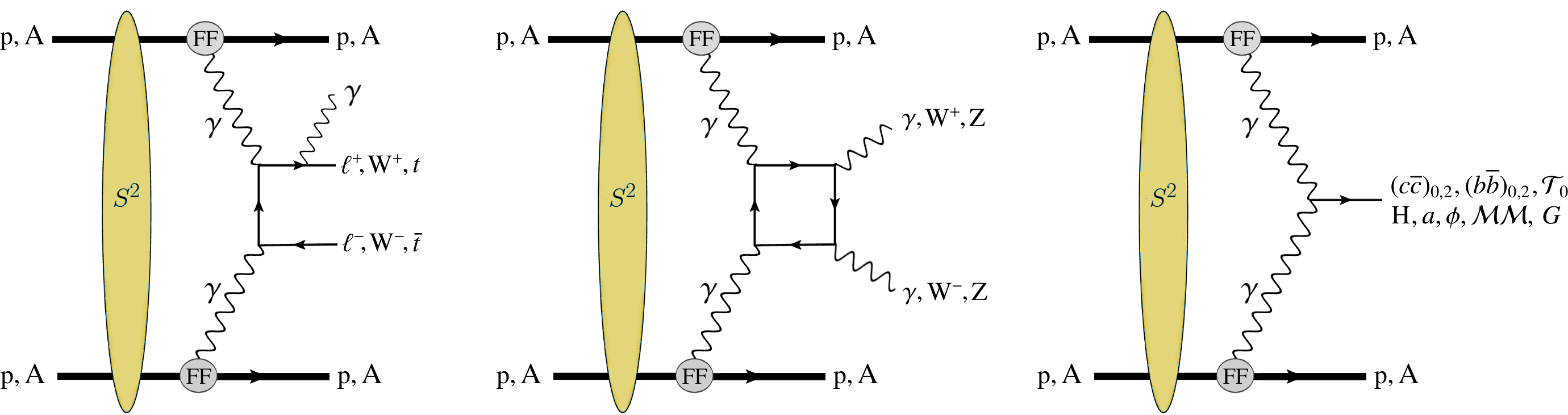
Figure 1: Typical exclusive $\gamma\gamma$ collision processes in UPCs of proton and ions (with form factors FF and survival probabilities $S^{2}$) that can be automatically generated with the gamma-UPC code: $t$-channel charged particle pair production with final-state photon radiation (left), box diagrams for diboson production (center), and resonant production of SM and BSM spin-even states (right).

Competitive searches for anomalous quartic gauge couplings (aQGC) dEnterria:2013zqi ; Pierzchala:2008xc , axion-like-particles (ALPs) Knapen:2016moh , Born–Infeld (BI) extensions of Quantum Electrodynamics (QED) Ellis:2017edi , or anomalous $\tau$ electromagnetic (e.m.) moments delAguila:1991rm ; Atag:2010ja ; Beresford:2019gww ; Dyndal:2020yen have thereby been performed, and many more studies of the Standard Model (SM) and beyond (BSM) are open to study in the near future Bruce:2018yzs ; Klein:2020nvu ; dEnterria:2022sut . Multiple SM and BSM $\gamma\gamma$ processes accessible in UPCs at hadron colliders are displayed in Fig. 1 and listed in Table 1.

Table 1: Gold-plated SM and BSM processes accessible via photon-photon collisions in UPCs at hadron colliders.

Process	Physics motivation
$\gamma\gamma\to e^{+}e^{-},\mu^{+}\mu^{-}$	“Standard candles” for proton/nucleus $\gamma$ fluxes, EPA calculations, and higher-order QED corrections
$\gamma\gamma\to\tau^{+}\tau^{-}$	Anomalous $\tau$ lepton e.m. moments delAguila:1991rm ; Atag:2010ja ; Beresford:2019gww ; Dyndal:2020yen
$\gamma\gamma\to\gamma\gamma$	aQGC dEnterria:2013zqi , ALPs Knapen:2016moh , BI QED Ellis:2017edi , noncommut. interactions Horvat:2020ycy , extra dims. Atag:2010bh ,…
$\gamma\gamma\to\mathcal{T}_{0}$	Ditauonium properties (heaviest QED bound state) dEnterria:2022ysg ; dEnterria:2022alo
$\gamma\gamma\to(c\overline{c})_{0,2},(b\overline{b})_{0,2}$	Properties of scalar and tensor charmonia and bottomonia  Yu:2017rfi ; Chapon:2020heu
$\gamma\gamma\to\mathrm{XYZ}$	Properties of spin-even XYZ heavy-quark exotic states Goncalves:2021ytq
$\gamma\gamma\to\mathrm{VM\,VM}$	(with $\mathrm{VM}=\rho,\omega,\phi,\,\mathrm{J}/\psi,\Upsilon$): BFKL-Pomeron dynamics Kwiecinski:1998sa ; Kwiecinski:1999hg ; Chernyak:2014wra ; Goncalves:2015sfy
$\gamma\gamma\to\mathrm{W}^{+}\mathrm{W}^{-},\,\mathrm{Z}\mathrm{Z},\,\mathrm{Z}\gamma,\cdots$	anomalous quartic gauge couplings Pierzchala:2008xc ; deFavereaudeJeneret:2009db ; Chapon:2009hh ; Baldenegro:2017aen
$\gamma\gamma\to\mathrm{H}$	Higgs-$\gamma$ coupling, total H width dEnterria:2009cwl ; dEnterria:2019jty
$\gamma\gamma\to\mathrm{HH}$	Higgs potential Belusevic:2004pz , quartic $\gamma\gamma\mathrm{HH}$ coupling
$\gamma\gamma\to t\overline{t}$	anomalous top-quark e.m. couplings deFavereaudeJeneret:2009db ; dEnterria:2009cwl
$\gamma\gamma\to\tilde{\ell}\tilde{\ell},\,\tilde{\chi}^{+}\tilde{\chi}^{-},\,\mathrm{H^{++}H^{--}}$	SUSY pairs: slepton deFavereaudeJeneret:2009db ; Beresford:2018pbt ; Harland-Lang:2018hmi , chargino deFavereaudeJeneret:2009db ; Godunov:2019jib , doubly-charged Higgs bosons deFavereaudeJeneret:2009db ; Babu:2016rcr .
$\gamma\gamma\to a,\phi,\mathcal{MM},\,G$	ALPs Knapen:2016moh ; Goncalves:2021pdc , radions Lietti:2002rq , monopoles Kurochkin:2006jr ; Dougall:2007tt ; Baines:2018ltl ; MoEDAL:2019ort , gravitons Atwood:1999zg ; Zhou:2007wfr ; Inan:2012zz ,…

The photons coherently emitted from a charged hadron must have a wavelength larger than the size of the latter, such that they do not resolve the individual hadron constituents (partons or nucleons in the case of protons or nuclei, respectively) but see the coherent action of them. Such coherence emission condition forces the photons to be almost on-mass shell, limiting their virtuality $Q^{2}=-q^{2}$ to very low values $Q^{2}<1/R^{2}$, where $R$ is the charge radius: $Q^{2}\approx~{}0.08$ GeV² for protons with $R\approx~{}0.7$ fm, and $Q^{2}<$ 4$\cdot 10^{-3}$ GeV² for nuclei with $R_{\mathrm{A}}\approx 1.2\,A^{1/3}$ fm, for mass number $A>$ 16. With the hadrons interacting only electromagnetically at large impact parameters without hadronic overlap, and surviving the emission of the quasireal photon, the $\gamma\gamma$ production processes are called exclusive or elastic (when only one hadron survives the UPC, the processes are called semiexclusive or semielastic). The photon spectra in the longitudinal direction have a typical $E_{\gamma}^{-1}$ bremsstrahlung-like spectrum up to energies of the order of $E_{\gamma}^{\text{max}}\approx\gamma_{\mathrm{L}}/R$, where $\gamma_{\mathrm{L}}=E_{\text{beam}}/m_{\text{p,N}}$ is the Lorentz relativistic factor of the proton (mass m${}_{\text{p}}$ = 0.9383 GeV) or ion (nucleon mass m${}_{\text{N}}$ = 0.9315 GeV), beyond which the $\gamma$ flux is further exponentially suppressed. The photon energies determine the rapidity of the produced system, $y=0.5\,\ln(E_{\gamma_{1}}/E_{\gamma_{2}})$, and the c.m. energy $W_{\gamma\gamma}=m_{\gamma\gamma}=\sqrt{4E_{\gamma_{1}}E_{\gamma_{2}}}$ which, for symmetric systems, is maximal at $y=0$ when $E_{\gamma_{1}}^{\text{max}}=E_{\gamma_{2}}^{\text{max}}\approx\gamma/b_{\text{min}}$ with $b_{\text{min}}$ the minimum impact parameter between the two charges of radius $R_{\mathrm{A,B}}$. Table 2 summarizes the typical parameters for p-p, p-A, and A-A UPCs at the LHC and Future Circular Collider (FCC) energies, illustrating the impressive range of maximum photon-photon c.m. energies $\sqrt{s_{{}_{\gamma\,\gamma}}}\approx 0.2$–30 TeV covered. The HL-LHC integrated luminosities for light-ion runs are taken from Bruce:2018yzs ; dEnterria:2022sut , although there are intriguing proposals to significantly enhance them for Ca-Ca collisions Krasny:2020wgx . Compared to the $e^{+}e^{-}$ and p-p cases, the main advantage of studies of photon-fusion processes via A-A UPCs is the lack of pileup collisions and the huge $Z^{2}$ photon-flux boost that leads to $\gamma\gamma$ cross sections comparatively enhanced by factors of up to $Z^{4}\approx 50\cdot 10^{6}$ for Pb-Pb. On the other hand, proton beams at the LHC feature $\mathcal{O}(10^{8})$ larger $\mathcal{L}_{\mathrm{\tiny{int}}}$, have forward proton detectors available to tag such collisions at high masses CMS:2021ncv ; Tasevsky:2015xya , and have harder $\gamma$ spectra compared to the heavy-ion case. All such p-p differences eventually compensate for the Pb-Pb advantages above $W_{\gamma\gamma}\equiv\sqrt{s_{{}_{\gamma\,\gamma}}}\approx~{}100$–300 GeV (depending on single- or double-proton tagging) CMS:2021ncv ; Bruce:2018yzs . Adding forward downstream proton spectrometers at 400 m in the LHC tunnel would cover collisions down to $W_{\gamma\gamma}\approx 50$ GeV FP420RD:2008jqg .

Table 2: Summary of the generic characteristics of photon-photon collisions in ultraperipheral proton and nuclear collisions at HL-LHC Bruce:2018yzs ; dEnterria:2022sut and FCC FCC:2018vvp ; Dainese:2016gch energies. For each colliding system, we quote its (i) nucleon-nucleon (NN) c.m. energy $\sqrt{s_{{}_{\text{NN}}}}$, (ii) integrated luminosity per typical run $\mathcal{L}_{\mathrm{\tiny{int}}}$, (iii) beam energies $\rm E_{beam}$, (iv) Lorentz factor $\gamma_{\mathrm{L}}$, (v) effective charge radius $R_{\mathrm{A}}$, (vi) photon “maximum” energy $E_{\gamma}^{\text{max}}$ in the c.m. frame, and (vii) “maximum” photon-photon c.m. energy $\sqrt{s_{\gamma\gamma}^{\text{max}}}$.

System	$\sqrt{s_{{}_{\text{NN}}}}$	$\mathcal{L}_{\mathrm{\tiny{int}}}$	$E_{\text{beam1}}+E_{\text{beam2}}$	$\gamma_{\mathrm{L}}$	$R_{\mathrm{A}}$	$E_{\gamma}^{\text{max}}$	$\sqrt{s_{\gamma\gamma}^{\text{max}}}$
Pb-Pb	5.52  TeV	5 nb-1	2.76 + 2.76 TeV	2960	7.1 fm	80 GeV	160 GeV
Xe-Xe	5.86 TeV	30 nb-1	2.93 + 2.93 TeV	3150	6.1 fm	100 GeV	200 GeV
Kr-Kr	6.46 TeV	120 nb-1	3.23 + 3.23 TeV	3470	5.1 fm	136 GeV	272 GeV
Ar-Ar	6.3  TeV	1.1 pb-1	3.15 + 3.15 TeV	3390	4.1 fm	165 GeV	330 GeV
Ca-Ca	7.0  TeV	0.8 pb-1	3.5 + 3.5 TeV	3760	4.1 fm	165 GeV	330 GeV
O-O	7.0  TeV	12.0 pb-1	3.5 + 3.5 TeV	3760	3.1 fm	240 GeV	490 GeV
p-Pb	8.8 TeV	1 pb-1	7.0 + 2.76 TeV	7450, 2960	0.7, 7.1 fm	2.45 TeV, 130 GeV	2.6 TeV
p-p	14 TeV	150 fb-1	7.0 + 7.0 TeV	7450	0.7 fm	2.45 TeV	4.5 TeV
Pb-Pb	39.4 TeV	110 nb-1	19.7 + 19.7 TeV	21 100	7.1 fm	600 GeV	1.2 TeV
p-Pb	62.8 TeV	29 pb-1	50. + 19.7 TeV	53 300, 21 100	0.7,7.1 fm	15.2 TeV, 600 GeV	15.8 TeV
p-p	100 TeV	1 ab-1	50. + 50. TeV	53 300	0.7 fm	15.2 TeV	30.5 TeV

Studies of photon-photon physics in UPCs with hadron beams at RHIC, LHC, and FCC have been so far carried out mostly employing dedicated Monte Carlo (MC) event generators such as Starlight Klein:2016yzr , Superchic Harland-Lang:2020veo , or fpmc (for p-p UPCs only) Boonekamp:2011ky , where a subset of selectable physical processes has been previously coded at leading-order (LO) QED accuracy. There is an increasing experimental and phenomenological need to have at hand more versatile MC generators that can automatically produce any final state of interest, including new SM and BSM signals, as well as any potential backgrounds (including, e.g., the generation of additional photon and/or gluon emissions from the final state particles), and that can be extended to include next-to-leading (NLO) pure QED or full electroweak (EW) corrections. Standard MC tools to automatically generate any collider final state of interest are MadGraph5_aMC@NLO (called MG5_aMC hereafter) Alwall:2011uj ; Alwall:2014hca for generic SM/BSM studies, and HELAC-Onia Shao:2012iz ; Shao:2015vga for dedicated studies of charmonium and bottomonium physics. At variance with the UPC-only MC generators, MG5_aMC and HELAC-Onia can not only produce any arbitrary final state but also generate events with additional higher-order real (photon and/or gluon) emissions, MG5_aMC is extendable to include also full NLO (real and virtual) EW corrections Frederix:2018nkq , and their full events are by default output in a convenient Les Houches Event (LHE) format Alwall:2006yp that can be automatically interfaced to external codes for the subsequent showering and hadronization (in the case of partonic final states) and/or decay of the produced particles.

In the case of p-p collisions, the MG5_aMC  generator already contains the possibility to produce arbitrary photon-induced final states via two different setups. The first one uses the inclusive photon distribution function (PDF) of the proton Frederix:2018nkq , such as the LuxQED Manohar:2016nzj , NNPDF31luxQED Bertone:2017bme , MMHT2015qed Harland-Lang:2019pla or CT18lux Xie:2021equ ones, where the photon is mostly emitted from the individual partons of the proton, which does not survive the QED interaction. The second setup, which is the main subject of this work, deals with the EPA case where only the coherent $\gamma$ emission by the proton is considered. The $\gamma$ flux currently implemented in MG5_aMC, dubbed “improved Weizsäcker-Williams” (iWW) (following Frixione:1993yw ), is obtained from the proton elastic electric ($E$) and magnetic ($M$) form factors in the dipole approximation, $F_{M}=G_{M}^{2}$ and $F_{E}=(4m_{\mathrm{p}}^{2}G_{E}^{2}+Q^{2}G_{M}^{2})/(4m_{\mathrm{p}}^{2}+Q^{2})$ where $G_{E}$ and $G_{M}$ are the “Sachs” form factors related by $G_{E}^{2}=G_{M}^{2}/7.78=(1+Q^{2}/Q_{0}^{2})^{-4}$, with $Q_{0}^{2}\approx 0.71\,\text{GeV}^{2}$. The photon number density as a function of the fraction of the proton energy carried by the photon, $x=E_{\gamma}/E_{\mathrm{p}}$, reads Budnev:1975poe

$$n_{\gamma/\mathrm{p}}^{\mathrm{iWW}}(x) = \frac{\alpha}{\pi}\,(1-x)\;\left[\varphi\left(x,Q^{2}_{\text{max}}/Q_{0}^{2}\right)-\varphi\left(x,Q^{2}_{\text{min}}/Q_{0}^{2}\right)\right]\;,\mbox{with}$$ (2)

$$\varphi(x,Q)=(1+c_{1}\,\vary)\,\left[-\ln\,\tfrac{1+Q}{Q}+\sum_{k=1}^{3}\tfrac{1}{k\,(1+Q)^{k}}\right]\,+\,\tfrac{(1-c_{2})\,\vary}{4Q(1+Q)^{3}}\,+c_{3}\,\left(1+\tfrac{\vary}{4}\right)\,\left[\ln\,\tfrac{(1+Q)-c_{2}}{1+Q}+\sum_{k=1}^{3}\tfrac{c_{2}^{k}}{k(1+Q)^{k}}\right]$$

where $\alpha=1/137.036$ is the QED coupling, $\vary=x^{2}/(1-x)$, and $c_{1}=(1+7.78)/4+4\,m_{\mathrm{p}}^{2}/Q_{0}^{2}\approx 7.16$, $c_{2}=1-4m_{\mathrm{p}}^{2}/Q_{0}^{2}\approx-3.96$, and $c_{3}=(7.78-1)/c_{2}^{4}\approx 0.028$ are constants. The minimum momentum transfer squared is a function of $x$ and the proton mass, $Q^{2}_{\text{min}}\approx(xm_{\mathrm{p}})^{2}/(1-x)$, and a value of $Q^{2}_{\text{max}}\approx 1$–2 GeV² is usually taken to warrant the “onshellness” of the photon. However, as we discuss below, the current MG5_aMC implementation of p-p UPCs deFavereaudeJeneret:2009db does not explicitly consider the survival of the protons, a fact that does not warrant the exclusivity condition of the final state. Accounting for such effects has been usually done by introducing a correction factor to the cross section, called the “survival probability” $S^{2}$ Dokshitzer:1987nc , which corresponds to the probability that both scattered protons do not dissociate due to secondary soft hadronic interactions (yellow “blob” in the Fig. 1 diagrams). Calculations of the survival factors are usually done in the impact parameter space, assuming factorization as in the EPA. Since the photon $Q$ is inversely proportional to the impact parameter of the p-p collision, which is usually much larger than the range of strong interactions, the proton survival probability in e.m. interactions has been so far de facto taken as $S^{2}_{\gamma\gamma}=1$ in MG5_aMC. However, since the average $Q^{2}$ increases with $\gamma$ energy, one expects a decreasing survival probability for processes with larger $W_{\gamma\gamma}$. Therefore, the current MG5_aMC EPA setup should be considered as just providing a reasonable upper value of the cross section for high-mass exclusive $\gamma\gamma$ processes in p-p UPCs.

This paper provides a description of the new ingredients that have been incorporated into the MG5_aMC and HELAC-Onia MC codes in order to be able to generate any exclusive photon-photon final state of interest, not only with proton but also with nuclear beams, including two modelings of the underlying hadronic form factors and associated survival probabilities (represented, respectively, by the grey circle and the yellow “blob” in the diagrams of Fig. 1). The paper is organized as follows. Section II provides a short reminder of the basic expressions to compute photon-fusion cross sections in the EPA framework. Section III describes the new gamma-UPC proton and heavy-ion EPA photon fluxes incorporated into MG5_aMC/HELAC-Onia based on the standard electric dipole form factor (EDFF) as well as on the charge form factor (ChFF), and associated survival factors for p-p, p-A, and A-A collisions. Results for a broad selection of exclusive $\gamma\gamma$ processes at hadron colliders are presented in Sections IV and V, including total cross sections for a large variety of resonances with even charge-conjugation ($C$) quantum number, BSM particles, as well as differential distributions for LbL and exclusive $\ell^{+}\ell^{-}$ production. Predictions for the latter are compared to the LHC data as well as to those of the Starlight and Superchic models. For all our calculations, the EDFF- and ChFF-based results are confronted and half the difference between their numerical cross sections is taken as indicative of the associated FF and $S^{2}$ uncertainties. Details on the gamma-UPC code output and ongoing developments of the framework to be implemented in upcoming releases are discussed in Section VI. The paper is closed with a summary in Section VII, and an appendix A with basic instructions to compile and run the code.

II Theoretical $\gamma\gamma$ cross sections

In the EPA framework, the exclusive production cross section of a final state $X$ via photon fusion in an UPC of hadrons A and B with charges $Z_{1,2}$, A  B $\xrightarrow{\gamma\gamma}$ A  $X$  B, factorizes into the product of the elementary cross section at a given $\gamma\gamma$ c.m. energy, $\sigma_{\gamma\gamma\to X}(W_{\gamma\gamma})$, convolved with the two-photon differential distribution of the colliding beams,

$$\sigma(\mathrm{A}\;\mathrm{B}\,\xrightarrow{\gamma\gamma}\mathrm{A}\;X\;\mathrm{B})=\int\frac{dE_{\gamma_{1}}}{E_{\gamma_{1}}}\frac{dE_{\gamma_{2}}}{E_{\gamma_{2}}}\,\frac{\mathrm{d}^{2}N^{(\mathrm{AB})}_{\gamma_{1}/\mathrm{Z}_{1},\gamma_{2}/\mathrm{Z}_{2}}}{\mathrm{d}E_{\gamma_{1}}\mathrm{d}E_{\gamma_{2}}}\sigma_{\gamma\gamma\to X}(W_{\gamma\gamma})\,.$$ (3)

where

$$\frac{\mathrm{d}^{2}N^{(\mathrm{AB})}_{\gamma_{1}/\mathrm{Z}_{1},\gamma_{2}/\mathrm{Z}_{2}}}{\mathrm{d}E_{\gamma_{1}}\mathrm{d}E_{\gamma_{2}}}=\int{\mathrm{d}^{2}\boldsymbol{b}_{1}\mathrm{d}^{2}\boldsymbol{b}_{2}\,P_{\text{no\,inel}}(\boldsymbol{b}_{1},\boldsymbol{b}_{2})\,N_{\gamma_{1}/\mathrm{Z}_{1}}(E_{\gamma_{1}},\boldsymbol{b}_{1})N_{\gamma_{2}/\mathrm{Z}_{2}}(E_{\gamma_{2}},\boldsymbol{b}_{2})}\,.$$ (4)

is derived from the convolution of the two photon number densities $N_{\gamma_{i}/\mathrm{Z}_{i}}(E_{\gamma_{i}},\boldsymbol{b}_{i})$ with energies $E_{\gamma_{1,2}}$ at impact parameters $\boldsymbol{b}_{1,2}$ from hadrons A and B, respectively; and $P_{\text{no\,inel}}(\boldsymbol{b}_{1},\boldsymbol{b}_{2})$ encodes the probability of hadrons A and B to remain intact after their interaction, which depends on their relative impact parameters. The $\gamma\gamma$ survival factor can then be written as

$$S^{2}_{\gamma\gamma}=\frac{\int{\mathrm{d}^{2}\boldsymbol{b}_{1}\mathrm{d}^{2}\boldsymbol{b}_{2}\,P_{\text{no\,inel}}(\boldsymbol{b}_{1},\boldsymbol{b}_{2})\,N_{\gamma_{1}/\mathrm{Z}_{1}}(E_{\gamma_{1}},\boldsymbol{b}_{1})N_{\gamma_{2}/\mathrm{Z}_{2}}(E_{\gamma_{2}},\boldsymbol{b}_{2})}}{\int{\mathrm{d}^{2}\boldsymbol{b}_{1}\mathrm{d}^{2}\boldsymbol{b}_{2}\,N_{\gamma_{1}/\mathrm{Z}_{1}}(E_{\gamma_{1}},\boldsymbol{b}_{1})N_{\gamma_{2}/\mathrm{Z}_{2}}(E_{\gamma_{2}},\boldsymbol{b}_{2})}},$$ (5)

where the numerator is the two-photon density accounting for finite-size effects, Eq. (4), and the denominator represents the integral of the two photon fluxes over all impact parameters without hadronic overlap constraint. The role of the modeling of $S^{2}_{\gamma\gamma}$ in p-p UPCs cross sections at the LHC has been discussed in Dyndal:2014yea ; Harland-Lang:2021ysd .

In the case of p-p UPCs calculations that ignore the hadronic-nonoverlap condition, the $\gamma$ flux has no explicit dependence on the impact parameter, i.e., $n_{\gamma}(E_{\gamma})=\int{N_{\gamma/\mathrm{p}}(E_{\gamma},\boldsymbol{b})\,\mathrm{d}^{2}\boldsymbol{b}}$, the survival factor is unity, and the two-photon distribution just factorizes as the product of two PDF-like photon distributions,

$$\frac{\mathrm{d}^{2}N^{(\mathrm{pp,factorized})}_{\gamma_{1}/\mathrm{Z}_{1},\gamma_{2}/\mathrm{Z}_{2}}}{\mathrm{d}E_{\gamma_{1}}\mathrm{d}E_{\gamma_{2}}}=n_{\gamma/\mathrm{p}}(x_{1})\,n_{\gamma/\mathrm{p}}(x_{2})\,,$$ (6)

where $n_{\gamma/\mathrm{p}}(x)$ is given by Eq. (2) for the EPA case, or by LuxQED-type PDFs for inclusive $\gamma\gamma$ collisions, in the current MG5_aMC implementation.

A particular case of interest in two-photon physics is the production of spin-0 and spin-2 resonances since, for real photons, the $\gamma\gamma\to$ vector process is forbidden by the Landau–Yang theorem Landau:1948kw ; Yang:1950rg . The cross section for the exclusive production of a $C$-even resonance $X$ (with spin $J$, and $\Gamma_{\gamma\gamma}(X)$ two-photon width) through $\gamma\gamma$ fusion in an UPC of charged particles A and B, is given by Budnev:1975poe

$$\sigma(\mathrm{A}\;\mathrm{B}\,\xrightarrow{\gamma\gamma}\mathrm{A}\;X\;\mathrm{B})=4\pi^{2}(2J+1)\frac{\Gamma_{\gamma\gamma}(X)}{m_{X}^{2}}\left.\frac{\mathrm{d}{\mathcal{L}}^{(\mathrm{A}\,\mathrm{B})}_{\gamma\gamma}}{\mathrm{d}W_{\gamma\gamma}}\right|_{W_{\gamma\gamma}=m_{X}},$$ (7)

where $\frac{d{\mathcal{L}}^{(\mathrm{A\,B})}_{\gamma\gamma}}{dW_{\gamma\gamma}}\big{|}_{W_{\gamma\gamma}=m_{X}}$ is the value of the effective two-photon luminosity at the resonance mass $m_{X}$, amounting to

$$\frac{\mathrm{d}{\mathcal{L}}^{(\mathrm{AB})}_{\gamma\gamma}}{\mathrm{d}W_{\gamma\gamma}} = \frac{2W_{\gamma\gamma}}{s_{{}_{\mathrm{NN}}}}\int{\frac{\mathrm{d}E_{\gamma_{1}}}{E_{\gamma_{1}}}\frac{\mathrm{d}E_{\gamma_{2}}}{E_{\gamma_{2}}}\delta\left(\frac{W_{\gamma\gamma}^{2}}{s_{{}_{\mathrm{NN}}}}-\frac{4E_{\gamma_{1}}E_{\gamma_{2}}}{s_{{}_{\mathrm{NN}}}}\right)\frac{\mathrm{d}^{2}N^{(\mathrm{AB})}_{\gamma_{1}/\mathrm{Z}_{1},\gamma_{2}/\mathrm{Z}_{2}}}{\mathrm{d}E_{\gamma_{1}}\mathrm{d}E_{\gamma_{2}}}}\,.$$ (8)

The expressions above, Eqs. (3)–(4) and Eqs. (7)–(8), are valid for any colliding system with the appropriate (charged lepton, proton, and/or heavy ion) photon fluxes and survival probabilities. For $e^{+}e^{-}$ beams, the photon flux in the WW approximation Kniehl:1996we is commonly used (also cf. Eq. (3) of Flore:2020jau ) in Eq. (6), with the maximum virtuality usually set to $Q^{2}_{\mathrm{max}}\approx 1$ GeV² when focusing on quasireal photon scatterings without the need to tag the $e^{\pm}$ transversely scattered at large angles. For proton beams one normally employs the $\gamma$ spectrum obtained from its elastic form factor, Eq. (2), whereas the impact-parameter-dependent expression from $b_{\text{min}}$ to infinity is used for the $\gamma$ spectrum of heavy ions Bertulani:1987tz . As aforementioned, in the case of proton and nuclear beams, an extra requirement needs however to be imposed to ensure that the collisions are truly exclusive, namely that they occur without hadronic interactions and subsequent breakup of the colliding particle beams. In the next section, we discuss the new photon fluxes and nonoverlap conditions incorporated into the MG5_aMC and HELAC-Onia generators.

III Effective photon-photon luminosities

At variance with photon-photon processes from pointlike emitters, the effective $\gamma\gamma$ luminosity in UPCs with hadrons cannot be just simply factorized as a direct convolution of the product of the photon densities of the two beams, such as in Eq. (6), because of their finite transverse profile and the consequent nonzero probability of concomitant hadronic interactions that can break the exclusivity condition. In past $\gamma\gamma$-fusion studies with MG5_aMC (see e.g. dEnterria:2009cwl ; dEnterria:2013zqi ; dEnterria:2019jty ), this effect has been often only partially accounted for either by imposing a maximum $Q^{2}_{\mathrm{max}}\approx 1$ GeV² value for the photon flux in p-p UPCs (a choice that de facto removes the most central $\gamma\gamma$ collisions with potential hadronic overlap), or by restricting the range of minimum impact parameters in the $\gamma$ fluxes to $b_{\text{min}}=R_{\mathrm{A,B}}$ plus an effective correction equivalent to the geometrical condition $|\boldsymbol{b}_{1}-\boldsymbol{b}_{2}|>R_{\mathrm{A}}+R_{\mathrm{B}}$ Cahn:1990jk in the case of p-A and A-A UPCs. A more realistic approach is considered here, similar to the ones implemented in the Starlight and Superchic MC generators. The two-photon differential yield (4), is now given by

$$\frac{\mathrm{d}^{2}N^{(\mathrm{AB})}_{\gamma_{1}/\mathrm{Z}_{1},\gamma_{2}/\mathrm{Z}_{2}}}{\mathrm{d}E_{\gamma_{1}}\mathrm{d}E_{\gamma_{2}}} = \int{\mathrm{d}^{2}\boldsymbol{b}_{1}\mathrm{d}^{2}\boldsymbol{b}_{2}\,P_{\text{no\,inel}}\left(\left|\boldsymbol{b}_{1}-\boldsymbol{b}_{2}\right|\right)\,N_{\gamma_{1}/\mathrm{Z}_{1}}(E_{\gamma_{1}},\boldsymbol{b}_{1})N_{\gamma_{2}/\mathrm{Z}_{2}}(E_{\gamma_{2}},\boldsymbol{b}_{2})\,\theta(b_{1}-\epsilon R_{\mathrm{A}})\theta(b_{2}-\epsilon R_{\mathrm{B}})}\,.$$ (9)

In this expression, $\theta(b_{1,2}-\epsilon R_{\mathrm{A,B}})$ is the Heaviside step function, and the $\epsilon>0$ parameter can be used to restrict the range of impact parameters depending on the concrete implementation of the photon EPA fluxes as explained below; and $P_{\text{no\,inel}}(b)$ is the probability to have no inelastic hadronic interaction at impact parameter $b$ given by standard opacity (optical density) or eikonal expressions Glauber:1970jm :

$$P_{\text{no\,inel}}\left(b\right) = \left\{\begin{array}[]{ll}e^{-\,\sigma^{\mathrm{NN}}_{\text{inel}}\cdot T_{\mathrm{AB}}(b)},&\text{for nucleus-nucleus UPCs}\\ e^{-\,\sigma^{\mathrm{NN}}_{\text{inel}}\cdot T_{\mathrm{A}}(b)},&\text{for proton-nucleus UPCs}\\ \left|1-\Gamma(s_{{}_{\text{NN}}},b)\right|^{2},\;\mbox{ with }\;\Upgamma(s_{{}_{\mathrm{NN}}},b)\propto e^{-b^{2}/(2b_{0})}&\text{for p-p\ UPCs}\\ \end{array}\right..$$ (13)

Here $T_{\mathrm{A}}(b)$ and $T_{\mathrm{AB}}(b)$ are the nuclear thickness and overlap functions respectively, commonly derived from the hadron transverse density profile via a Glauber MC model Loizides:2017ack ; dEnterria:2020dwq , $\sigma^{\mathrm{NN}}_{\text{inel}}\equiv\sigma^{\mathrm{NN}}_{\text{inel}}(\!\sqrt{s_{{}_{\text{NN}}}})$ is the inelastic NN scattering cross section parametrized as a function of $\sqrt{s_{{}_{\text{NN}}}}$ as in dEnterria:2020dwq , and $\Upgamma(s_{{}_{\mathrm{NN}}},b)$ is the Fourier transform of the p-p elastic scattering amplitude modelled by an exponential function Frankfurt:2006jp with inverse slope $b_{0}\equiv b_{0}(\!\sqrt{s_{{}_{\text{NN}}}})$ dependent on the NN c.m. energy. Figure 2 shows a compilation of all measurements of the $b_{0}$ slope extracted in elastic scattering measurements at low $-t\lesssim 0.3$ GeV² in p-p TOTEM:2012oyl ; TOTEM:2013lle ; TOTEM:2017asr ; TOTEM:2018psk ; STAR:2020phn ; ATLAS:2014vxr ; ATLAS:2016ygv and p-$\overline{\mathrm{p}}$ ParticleDataGroup:2010dbb collisions as a function of $\sqrt{s_{{}_{\text{NN}}}}$. In principle, the elastic slope is defined at zero exchanged momenta ($t=0$), but the experimental determinations of $b_{0}$ depend on the actual chosen $|t|$-range used to extract it, and whether or not local deviations of the data from a pure exponential due to Coulomb-nuclear interference are taken into account. These facts explain some of the relative large dispersion of slopes measured at the same $\sqrt{s}$ value, and uncertainties beyond the plotted experimental error bars should be expected in some cases. The experimental data have been fit here to the functional form $b_{0}(\sqrt{s_{{}_{\text{NN}}}})=A+B\,\ln(s_{{}_{\text{NN}}})+C\ln^{2}(s_{{}_{\text{NN}}})$, yielding $A=9.81$ GeV^-2, $B=0.211$ GeV^-2, and $C=0.0185$ GeV^-2 (for $s_{{}_{\text{NN}}}$ measured in GeV²) with goodness-of-fit per degree-of-freedom of $\chi^{2}/N_{\mathrm{dof}}=2.3$. Whereas a simple logarithmic dependence $\ln(s_{{}_{\text{NN}}})$ is expected in the case of one-Pomeron exchange, the fit needs an extra $\ln^{2}(s_{{}_{\text{NN}}})$ term to reproduce the highest c.m. energy data, a manifestation of the increasing role of multi-Pomeron exchanges at LHC energies and beyond Schegelsky:2011aa . Such a fit predicts $b_{0}=20.6,24.5$ GeV^-2 for p-p collisions at LHC(14 TeV) and FCC(100 TeV), respectively. The photon number densities, $N_{\gamma/\mathrm{Z}}(E_{\gamma},b)$, the key ingredient of Eq. (9), have been implemented as discussed next.

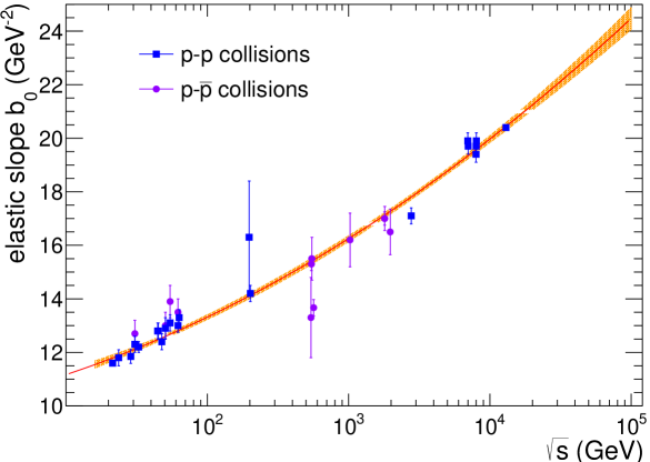
Figure 2: Measurements of the low-$|t|$ exponential elastic slope $b_{0}$ in p-p TOTEM:2012oyl ; TOTEM:2013lle ; TOTEM:2017asr ; TOTEM:2018psk ; STAR:2020phn ; ATLAS:2014vxr ; ATLAS:2016ygv and p-$\overline{\mathrm{p}}$ ParticleDataGroup:2010dbb collisions as a function of $\sqrt{s}=\sqrt{s_{{}_{\text{NN}}}}$ (individual data points at the same $\sqrt{s}$ have been slightly shifted to the left or right to improve visibility). The orange curve shows our fit to the data, $b_{0}=A+B\,\ln(s_{{}_{\text{NN}}})+C\ln^{2}(s_{{}_{\text{NN}}})$, with the parameters given in the text.

The first $\gamma$ flux considered in this work, and commonly used in the literature, is derived from the electric dipole form factor (EDFF) of the emitting hadron. For ion beams with charge number $Z$ and Lorentz boost $\gamma_{\mathrm{L}}$, the photon number density at impact parameter $b$ obtained from its corresponding EDFF reads

$$N^{\text{EDFF}}_{\gamma/\mathrm{Z}}(E_{\gamma},b) = \frac{Z^{2}\alpha}{\pi^{2}}\frac{\xi^{2}}{b^{2}}\left[K_{1}^{2}(\xi)+\frac{1}{\gamma_{\mathrm{L}}^{2}}K_{0}^{2}(\xi)\right]\,,$$ (14)

where $\xi=E_{\gamma}b/\gamma_{\mathrm{L}}$, and $K_{i}$’s are modified Bessel functions Baltz:2007kq . The first term inside the parentheses gives the flux of transversely polarized photons with respect to the ion direction, which dominates for relativistic nuclei, while the second one is the flux for longitudinally polarized photons. As aforementioned, the flux is exponentially suppressed for $E_{\gamma}\gtrsim\gamma_{\mathrm{L}}/b$ (corresponding to the $E_{\gamma}^{\mathrm{max}}$ values of Table 2). Since the EDFF photon number density is divergent when $b\to 0$ (Fig. 3, blue dashed curves), the $\epsilon$ parameter in the integral Eq. (9) is usually taken as unity ($\epsilon^{\text{EDFF}}=1$), which is equivalent to restricting the integration to impact parameters $b_{1,2}>R_{\mathrm{A,B}}$ (vertical dashed lines in Fig. 3, where we have taken the radius parameters as those of the corresponding Woods-Saxon nuclear profiles in Table 3).

For proton UPC fluxes, the same expression (14) is applicable using $Z=1$. However, the EDFF flux for protons assuming 100% survival probability (setting $P_{\text{no\,inel}}=1$ in Eq. (5)) is not identical to the $b$-independent flux given by Eq. (2). Indeed, for $P_{\text{no\,inel}}=1$, one can analytically integrate (14) over $b$, and obtain the effective photon PDF as

$$n_{\gamma/\mathrm{p}}^{\mathrm{EDFF}}(x)=n_{\gamma/\mathrm{p}}(xR_{\mathrm{p}}m_{\mathrm{p}}),\;\mbox{ with }\;n_{\gamma/\mathrm{p}}(\chi)=\frac{2\alpha}{\pi}\left[\chi K_{0}(\chi)K_{1}(\chi)-\left(1-\gamma_{\mathrm{L}}^{-2}\right)\frac{\chi^{2}}{2}\left(K_{1}^{2}(\chi)-K_{0}^{2}(\chi)\right)\right]\,,$$ (15)

which is different than $n_{\gamma/\mathrm{p}}^{\mathrm{iWW}}(x)$ in Eq. (2) that keeps an explicit dependence on the photon (maximum and minimum) virtualities.

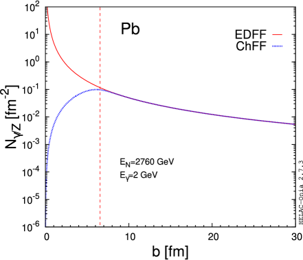
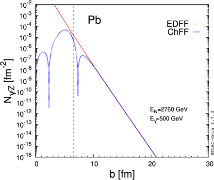
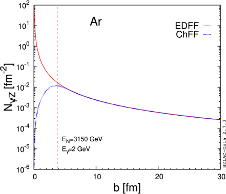
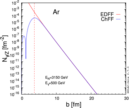
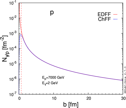
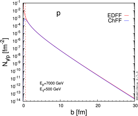
Figure 3: Comparison of the photon number densities at low ($E_{\gamma}=2$ GeV, left) and high ($E_{\gamma}=500$ GeV, right) energies as functions of the impact parameter $b$, obtained with the two form factors considered here (EDFF, red solid, and ChFF, blue dashed) for Pb ions at $2.76$ TeV (top), Ar at $3.15$ TeV (middle), and proton at $7$ TeV (bottom). The vertical dashed red lines at $b\approx R_{\mathrm{A}}$ indicate the threshold lower-limit imposed on the integral of the EDFF fluxes.

The second photon flux implemented in our code is that derived from the integral over the charge form factor (ChFF) of the nucleus Vidovic:1992ik [cf. Eq. (43) there], i.e.,

$$N^{\text{ChFF}}_{\gamma/\mathrm{Z}}(E_{\gamma},b) = \frac{Z^{2}\alpha}{\pi^{2}}\left|\int_{0}^{+\infty}{\frac{dk_{\perp}k_{\perp}^{2}}{k_{\perp}^{2}+E_{\gamma}^{2}/\gamma_{\mathrm{L}}^{2}}F_{\text{ch,A}}\left(\sqrt{k_{\perp}^{2}+E_{\gamma}^{2}/\gamma_{\mathrm{L}}^{2}}\right)}\,J_{1}\left(bk_{\perp}\right)\right|^{2}\,,$$ (16)

where $F_{\text{ch,A}}$ is the ChFF of the ion A emitting the photon, $k_{\perp}$ is the photon transverse momentum, related to its virtuality as $Q^{2}=k_{\perp}^{2}+E_{\gamma}^{2}/\gamma_{\mathrm{L}}^{2}$, and $J_{1}$ is the Bessel function of the first kind. The ChFF can be related to the transverse density profile of the radiating ion A, via

$$F_{\text{ch,A}}(q) = \int{\mathrm{d}^{3}\boldsymbol{r}e^{i\boldsymbol{q}\cdot\boldsymbol{r}}\rho_{\mathrm{A}}(\boldsymbol{r})}=\frac{4\pi}{q}\int_{0}^{+\infty}{\mathrm{d}r\rho_{\mathrm{A}}(r)r\sin{\left(qr\right)}}\,,$$ (17)

with $q=\sqrt{k_{\perp}^{2}+m_{\mathrm{N}}^{2}x^{2}}$, where the particle density $\rho_{\mathrm{A}}$ is normalized to unity

$$\int{\mathrm{d}^{3}\boldsymbol{r}\rho_{\mathrm{A}}(\boldsymbol{r})} = 1,$$ (18)

and the last equality of (17) applies for isotropic $\rho_{\mathrm{A}}$ densities. A more generic density profile of nuclei is given by the $3$-parameter Woods-Saxon function DeJager:1974liz ; DeVries:1987atn

$$\rho_{\mathrm{A}}(r) = \rho_{\mathrm{0,\mathrm{A}}}\frac{1+w_{\mathrm{A}}\left(r/R_{\mathrm{A}}\right)^{2}}{1+\exp{\left(\frac{r-R_{\mathrm{A}}}{a_{\mathrm{A}}}\right)}},$$ (19)

with $\rho_{\mathrm{0,\mathrm{A}}}$ a normalization constant so that Eq. (18) is fulfilled, and typical radial parameters ($R_{\mathrm{A}}$, $a_{\mathrm{A}}$, and $w_{\mathrm{A}}$) listed in Table 3 for various nuclei.

Table 3: Parameters of the Woods-Saxon profile, Eq. (19), for a variety of nuclei implemented in our code. For each ion we quote its mass number, charge, and radial parameters $R_{\mathrm{A}}$, $a_{\mathrm{A}}$, and $w_{\mathrm{A}}$ from Refs. DeJager:1974liz ; DeVries:1987atn ; Loizides:2017ack .

Nucleus	$A$	$Z$	$R_{\mathrm{A}}$ [fm]	$a_{\mathrm{A}}$ [fm]	$w_{\mathrm{A}}$
O	16	8	$2.608$	$0.513$	$-0.051$
Ar	40	18	$3.766$	$0.586$	$-0.161$
Ca	40	20	$3.766$	$0.586$	$-0.161$
Kr	78	36	$4.5$	$0.5$	$0$
Xe	129	54	$5.36$	$0.59$	$0$
Pb	208	82	$6.624$	$0.549$	$0$

Plugging into Eq. (17) the 3-parameter Woods-Saxon function above, the following analytic ChFF formula can be derived:

$$F_{\text{ch},A}(q) = \frac{4\pi^{2}\rho_{0,\mathrm{A}}a_{\mathrm{A}}^{3}}{q^{2}a_{\mathrm{A}}^{2}\sinh^{2}{(\pi qa_{\mathrm{A}})}}\left\{\pi qa_{\mathrm{A}}\cosh{(\pi qa_{\mathrm{A}})}\sin{(qR_{\mathrm{A}})}\left[1-\frac{w_{\mathrm{A}}a_{\mathrm{A}}^{2}}{R_{\mathrm{A}}^{2}}\left(\frac{6\pi^{2}}{\sinh^{2}{(\pi qa_{\mathrm{A}})}}+\pi^{2}-3\frac{R_{\mathrm{A}}^{2}}{a_{\mathrm{A}}^{2}}\right)\right]\right.$$ (20)

$$\left.-qR_{\mathrm{A}}\sinh{(\pi qa_{\mathrm{A}})}\cos{(qR_{\mathrm{A}})}\left[1-\frac{w_{\mathrm{A}}a_{\mathrm{A}}^{2}}{R_{\mathrm{A}}^{2}}\left(\frac{6\pi^{2}}{\sinh^{2}{(\pi qa_{\mathrm{A}})}}+3\pi^{2}-\frac{R_{\mathrm{A}}^{2}}{a_{\mathrm{A}}^{2}}\right)\right]\right\}$$

$$+\underbrace{8\pi\hat{\rho}_{0,\mathrm{A}}a_{\mathrm{A}}^{3}\sum_{n=1}^{+\infty}{(-1)^{n-1}\frac{ne^{-n\frac{R_{\mathrm{A}}}{a_{\mathrm{A}}}}}{\left(n^{2}+q^{2}a_{\mathrm{A}}^{2}\right)^{2}}\left[1+12\frac{w_{\mathrm{A}}a_{\mathrm{A}}^{2}}{R_{\mathrm{A}}^{2}}\frac{n^{2}-q^{2}a_{\mathrm{A}}^{2}}{(n^{2}+q^{2}a_{\mathrm{A}}^{2})^{2}}\right]}}_{F_{\text{ch},A,2}(q)}$$

$$= F_{\text{ch},A,1}(q)+F_{\text{ch},A,2}(q),$$

which has been conveniently split into the last sum of two terms because the expression for $w_{\mathrm{A}}=0$ is already known from Ref. Maximon:1966sqn [cf. Eqs. (1) and (20) there], and we are also able to analytically work out the integral in Eq. (16) for the second term $F_{\text{ch,A,2}}(q)$, as follows

$$\int_{0}^{+\infty}{\frac{dk_{\perp}k_{\perp}^{2}}{k_{\perp}^{2}+\frac{E_{\gamma}^{2}}{\gamma_{\mathrm{L}}^{2}}}F_{\text{ch},A,2}\left(\sqrt{k_{\perp}^{2}+\frac{E_{\gamma}^{2}}{\gamma_{\mathrm{L}}^{2}}}\right)J_{1}(bk_{\perp})}=$$ (21)

$$= \frac{E_{\gamma}}{\gamma_{\mathrm{L}}}8\pi\rho_{0,\mathrm{A}}a_{\mathrm{A}}^{3}\sum_{n=1}^{+\infty}{(-1)^{n-1}ne^{-n\frac{R_{\mathrm{A}}}{a_{\mathrm{A}}}}\left\{\left[\frac{K_{1}(\xi)}{n^{4}}-\sqrt{1+n^{2}\tilde{a}_{\mathrm{A}}^{-2}}\frac{K_{1}\left(\tilde{B}_{n}\right)}{n^{4}}-\frac{\xi}{2n^{2}\tilde{a}_{\mathrm{A}}^{2}}K_{0}\left(\tilde{B}_{n}\right)\right]\right.}$$

$$+12\frac{w_{\mathrm{A}}a_{\mathrm{A}}^{2}}{R_{\mathrm{A}}^{2}}\left[\frac{K_{1}(\xi)}{n^{6}}-\left(\frac{1}{n^{6}}+\frac{\xi^{2}(5n^{2}+3\tilde{a}_{\mathrm{A}}^{2})}{24n^{2}(n^{2}+\tilde{a}_{\mathrm{A}}^{2})^{2}\tilde{a}_{\mathrm{A}}^{2}}\right)\sqrt{1+n^{2}\tilde{a}_{\mathrm{A}}^{-2}}K_{1}(\tilde{B}_{n})\right.\left.\left.-\left(\frac{\xi}{2n^{4}\tilde{a}_{\mathrm{A}}^{2}}+\frac{\xi^{3}}{24(\tilde{a}_{\mathrm{A}}^{2}+n^{2})\tilde{a}_{\mathrm{A}}^{4}}\right)K_{0}(\tilde{B}_{n})\right]\right\}$$

$$= -\frac{E_{\gamma}}{\gamma_{\mathrm{L}}}8\pi\rho_{0,\mathrm{A}}a_{\mathrm{A}}^{3}K_{1}(\xi)\left[\text{Li}_{3}\left(-e^{-\frac{R_{\mathrm{A}}}{a_{\mathrm{A}}}}\right)+12\frac{w_{\mathrm{A}}a_{\mathrm{A}}^{2}}{R_{\mathrm{A}}^{2}}\text{Li}_{5}\left(-e^{-\frac{R_{\mathrm{A}}}{a_{\mathrm{A}}}}\right)\right]$$

$$+\frac{E_{\gamma}}{\gamma_{\mathrm{L}}}8\pi\rho_{0,\mathrm{A}}a_{\mathrm{A}}^{3}\sum_{n=1}^{+\infty}{(-1)^{n-1}ne^{-n\frac{R_{\mathrm{A}}}{a_{\mathrm{A}}}}\left\{\left[-\sqrt{1+n^{2}\tilde{a}_{\mathrm{A}}^{-2}}\frac{K_{1}\left(\tilde{B}_{n}\right)}{n^{4}}-\frac{\xi}{2n^{2}\tilde{a}_{\mathrm{A}}^{2}}K_{0}\left(\tilde{B}_{n}\right)\right]\right.}$$

$$+12\frac{w_{\mathrm{A}}a_{\mathrm{A}}^{2}}{R_{\mathrm{A}}^{2}}\left[-\left(\frac{1}{n^{6}}+\frac{\xi^{2}(5n^{2}+3\tilde{a}_{\mathrm{A}}^{2})}{24n^{2}(n^{2}+\tilde{a}_{\mathrm{A}}^{2})^{2}\tilde{a}_{\mathrm{A}}^{2}}\right)\sqrt{1+n^{2}\tilde{a}_{\mathrm{A}}^{-2}}K_{1}(\tilde{B}_{n})\right.\left.\left.-\left(\frac{\xi}{2n^{4}\tilde{a}_{\mathrm{A}}^{2}}+\frac{\xi^{3}}{24(\tilde{a}_{\mathrm{A}}^{2}+n^{2})\tilde{a}_{\mathrm{A}}^{4}}\right)K_{0}(\tilde{B}_{n})\right]\right\},$$

where we have used the notations $\tilde{a}_{\mathrm{A}}=a_{\mathrm{A}}\,E_{\gamma}/\gamma_{\mathrm{L}}$ and $\tilde{B}_{n}=\xi\sqrt{1+n^{2}\tilde{a}_{\mathrm{A}}^{-2}}$, and $\text{Li}_{m}$’s are standard polylogarithms of order $m$. We opt for numerically integrating $F_{\text{ch},A,1}$ in Eq. (16), which is however nontrivial because the integrand involves highly oscillatory trigonometric functions and the $J_{1}$ Bessel function. Finally, we can solve $\rho_{0,\mathrm{A}}$ from the normalization condition Eq. (18), yielding

$$\rho_{0,\mathrm{A}} = \frac{1}{-8\pi a_{\mathrm{A}}^{3}\left[\text{Li}_{3}\left(-e^{\frac{R_{\mathrm{A}}}{a_{\mathrm{A}}}}\right)+12\frac{w_{\mathrm{A}}a_{\mathrm{A}}^{2}}{R_{\mathrm{A}}^{2}}\text{Li}_{5}\left(-e^{\frac{R_{\mathrm{A}}}{a_{\mathrm{A}}}}\right)\right]}\,.$$ (22)

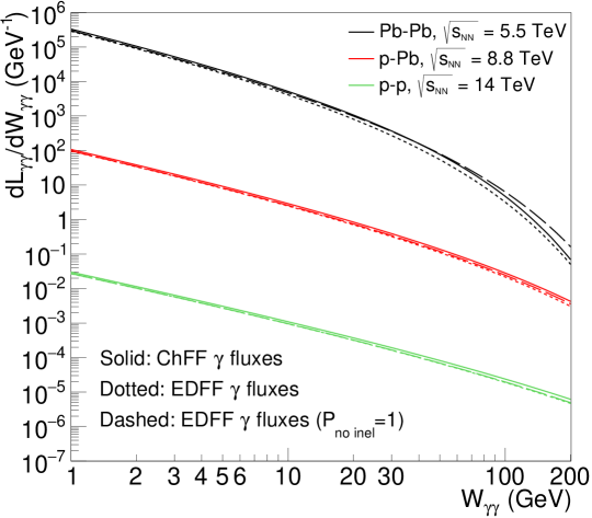
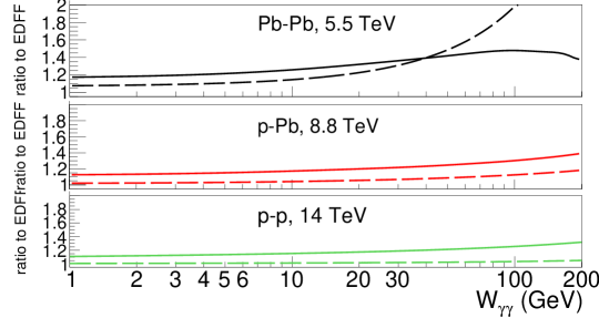
Figure 4: Comparison of the effective photon-photon luminosities $\mathrm{d}{\mathcal{L}}_{\gamma\gamma}/\mathrm{d}W_{\gamma\gamma}$ as a function of $W_{\gamma\gamma}$, Eq. (8), for ultraperipheral Pb-Pb, p-Pb, and p-p collisions at the LHC. The solid curves are obtained using ChFF, the dotted curves using EDFF, and the dashed curves using EDFF fluxes with $P_{\text{no\,inel}}=1$. The lower insets show the corresponding ratios over the EDFF-based luminosities.

For the proton case, we implement in Eq. (16) the dipole form factor Klein:2003vd

$$F_{\text{ch},\mathrm{p}}(q) = \frac{1}{\left(1+q^{2}a_{\mathrm{p}}^{2}\right)^{2}}$$ (23)

with $a_{\mathrm{p}}^{-2}=Q_{0}^{2}=0.71~{}\text{GeV}^{2}$, resulting in the following ChFF $\gamma$ number density for the proton

$$N_{\gamma/\mathrm{p}}^{\text{ChFF}}(E_{\gamma},b) = \frac{\alpha}{\pi^{2}}\frac{\xi^{2}}{b^{2}}\left\{\left[K_{1}(\xi)-\sqrt{1+\tilde{a}_{\mathrm{p}}^{-2}}K_{1}\left(\xi\sqrt{1+\tilde{a}_{\mathrm{p}}^{-2}}\right)\right]-\frac{\xi}{2\tilde{a}_{\mathrm{p}}^{2}}K_{0}\left(\xi\sqrt{1+\tilde{a}_{\mathrm{p}}^{-2}}\right)\right\}^{2}\,,$$ (24)

where $\tilde{a}_{\mathrm{p}}=a_{\mathrm{p}}\,E_{\gamma}/\gamma_{\mathrm{L}}$. In the limit $a_{\mathrm{p}}\to 0$, the ChFF flux reproduces the transversely polarized part of the EDFF flux, Eq. (14).

For the charge form factor, we can safely set the $\epsilon$ parameter to zero in Eq. (9), i.e., $\epsilon^{\text{ChFF}}=0$, because the photon number densities are well-behaved for $b\to 0$, as can be seen by the blue dashed lines in Fig. 3. The ChFF is more realistic than the EDFF as it allows considering also the photon flux within the nuclei, namely for $b<R_{\mathrm{A}}$, which e.g. enables the interpretation of the exclusive dimuon ATLAS measurement Burmasov:2021phy , as pointed out earlier by Ref. Baltz:2009jk . We stress the difference with respect to Ref. Burmasov:2021phy , as we have extended the fluxes for the generic $w_{\mathrm{A}}\neq 0$ ion profile case, and also kept the higher-order terms in $e^{-n\frac{R_{\mathrm{A}}}{a_{\mathrm{A}}}}$ for $n>1$ in the ChFF $F_{\text{ch},A}(q)$ function.

Figure 3 shows the EDFF (red solid) and ChFF (blue dashed) photon number densities for Pb (top), Ar (middle), and p (bottom) ions at LHC energies, for two indicative low ($E_{\gamma}=2$ GeV) and very high ($E_{\gamma}=500$ GeV) photon energies. The fluxes have clearly different shapes at low impact parameters: a continuous powerlaw-like decrease (divergent for $b\to 0$) in the EDFF case, and a rising ChFF flux with impact parameter up to a few fm followed by a falloff that is very similar to the EDFF one. However, the $b_{1,2}>R_{\mathrm{A,B}}$ requirement (indicated by the vertical dashed lines in the plots) implemented in the EDFF two-photon integral, Eq. (9), renders such low-$b$ flux differences with the ChFF case less relevant in terms of actual photon-photon luminosities. At very high $\gamma$ energies, one can see that the ChFF fluxes for heavy ions show an oscillatory pattern, which is however unlikely to have any experimental impact given the large beam luminosities needed to reach such high $E_{\gamma}$ values.

The effective photon-photon luminosities $\mathrm{d}{\mathcal{L}}_{\gamma\gamma}/\mathrm{d}W_{\gamma\gamma}$ for p-p, p-Pb, and Pb-Pb UPCs at the LHC, as obtained from Eq. (8) using the EDFF (with and without the hadronic nonoverlap requirement) and ChFF functions, are shown in Fig. 4. In the lower insets of Fig. 4, the corresponding ratios over the EDFF $\gamma\gamma$ luminosity results are plotted. The first observation is that, as expected, the $P_{\text{no\,inel}}\neq 1$ requirement (dashed curves) reduces the photon-photon luminosities for increasing $W_{\gamma\gamma}$ values (i.e., for lower impact parameters), in particular for Pb-Pb UPCs where the nonoverlap condition depletes the effective luminosity by 50% above $W_{\gamma\gamma}\approx 50$ GeV, and by about a factor of three above 200 GeV (the impact of the nonoverlap requirement for the $\gamma\gamma$ luminosity of p-p collisions is much smaller, leading to a 1–5% reduction over the considered mass range). The second observation is that the ChFF-based luminosities (solid curves) are overall larger than their EDFF counterparts by 10–30% for p-p and p-Pb UPCs, and by 15–50% for Pb-Pb UPCs for small–large masses, respectively. As we will see in the next section, this implies that the ChFF cross sections for increasingly heavier final states are larger by about 10–20% (for p-p and p-Pb UPCs at the LHC) and 20–40% (for Pb-Pb UPCs at the LHC) than the EDFF ones. In addition, Fig. 5 shows a comparison of the EDFF and ChFF effective photon-photon luminosities $\mathrm{d}{\mathcal{L}}_{\gamma\gamma}/\mathrm{d}W_{\gamma\gamma}$ derived for UPCs with lighter heavy-ion systems at the LHC (Xe-Xe, Kr-Kr, Ar-Ar, Ca-Ca, and O-O; left), and for p-p, p-Pb, and Pb-Pb UPCs at the FCC (right). All such colliding systems are incorporated by default in the gamma-UPC code. The theoretical precision of the EDFF- and ChFF-based predictions are being quantitatively estimated by varying all underlying gamma-UPC model input parameters within their uncertainties, and will be presented in an upcoming work inpreparation .

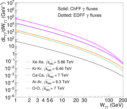
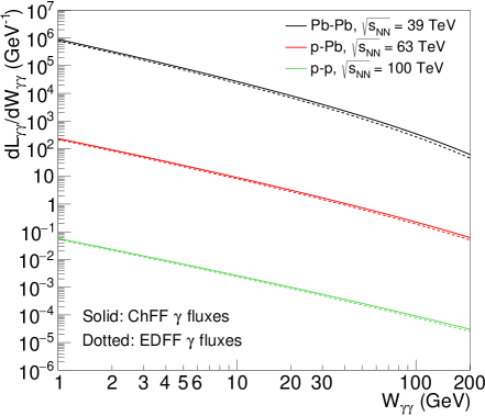
Figure 5: Comparison of the effective photon-photon luminosities $\mathrm{d}{\mathcal{L}}_{\gamma\gamma}/\mathrm{d}W_{\gamma\gamma}$ as a function of $W_{\gamma\gamma}$, Eq. (8), for UPCs of various ion species at the LHC (left) and for p-p, p-Pb, and Pb-Pb collisions at the FCC (right). Solid and dotted curves are obtained using ChFF and EDFF photon fluxes, respectively.

IV Total photon-photon cross sections results

In this section we present predictions for total photon-fusion cross sections at LHC and FCC energies for a large variety of spin-even (scalar or tensor) resonances; for pairs of $\mathrm{J}/\psi$ mesons, W bosons, Z bosons, and top quarks; and for axionlike particles and massive gravitons; all produced in p-p, p-A, and A-A UPCs. In all cases, results derived with EDFF and ChFF photon fluxes are presented.

IV.1 $C$-even resonances

Table 4: List of all known $C$-even resonances above $m_{X}\approx 3$ GeV that can be produced via two-photon fusion. For each particle, we quote its $J^{PC}$ quantum numbers, mass $m_{X}$, and diphoton partial width $\Gamma_{\gamma\gamma}$ from measurements Zyla:2020zbs or theoretical predictions (for $\mathrm{\eta_{b}(2\mathrm{S})}$, $\mathrm{\chi_{b0}},\mathrm{\chi_{b2}}$, $\mathcal{T}_{0}$, and H, see text for details).

Resonance	$J^{PC}$	$m_{X}$ (GeV)	$\Gamma_{\gamma\gamma}$ (MeV)
$\mathrm{\eta_{c}(1\mathrm{S})}$	$0^{-+}$	$2.9839\pm 0.0005$	$(5.06\pm 0.34)\cdot 10^{-3}$
$\mathrm{\eta_{c}(2\mathrm{S})}$	$0^{-+}$	$3.6375\pm 0.0011$	$(2.15\pm 1.47)\cdot 10^{-3}$
$\mathrm{\chi_{c0}}$	$0^{++}$	$3.41471\pm 0.00030$	$(2.203\pm 0.097)\cdot 10^{-3}$
$\mathrm{\chi_{c2}}$	$2^{++}$	$3.55617\pm 0.00007$	$(5.614\pm 0.197)\cdot 10^{-4}$
$\mathcal{T}_{0}$	$0^{-+}$	$3.5537\pm 0.0002$	$1.83\cdot 10^{-8}$
$\mathrm{\eta_{b}(1\mathrm{S})}$	$0^{-+}$	$9.3987\pm 0.0020$	$(4.8^{+2.5}_{-2.0})\cdot 10^{-4}$
$\mathrm{\eta_{b}(2\mathrm{S})}$	$0^{-+}$	$9999\pm 4$	$(2.4^{+1.2}_{-1.0})\cdot 10^{-4}$
$\mathrm{\chi_{b0}}$	$0^{++}$	$9.85944\pm 0.00052$	$(0.15^{+0.05}_{-0.03})\cdot 10^{-3}$
$\mathrm{\chi_{b2}}$	$2^{++}$	$9.91221\pm 0.00040$	$(9.3^{+1.3}_{-6.2})\cdot 10^{-6}$
H	$0^{++}$	$125.250\pm 0.170$	$(9.3\pm 0.2)\cdot 10^{-3}$

The cross section for the exclusive production of a $C$-even resonance $X$ through $\gamma\gamma$ fusion in an UPC is given by Eq. (7), and is completely determined from its spin $J=0,2$, two-photon width $\Gamma_{\gamma\gamma}(X)$, and the photon-photon effective luminosity of the colliding system at the particle mass. In Table 4, we list the relevant properties of all presently known scalar and tensor resonances from $m_{X}\approx 3$ GeV up to the Higgs boson. Except for the Higgs and ditauonium cases, the rest of spin-even particles over this mass range are charmonium and bottomonium bound states. Masses are precisely determined for all the particles, although not all their two-photon widths have been experimentally measured Zyla:2020zbs . All charmonium resonances have diphoton widths known to within 3–6% except for $\mathrm{\eta_{c}(2\mathrm{S})}$, which is badly known and has a $\pm 60\%$ uncertainty presently. The $\gamma\gamma$ decays of four $b\overline{b}$ resonances ($\mathrm{\eta_{b}(1\mathrm{S})}$, $\mathrm{\eta_{b}(2\mathrm{S})}$, $\mathrm{\chi_{b0}}$, $\mathrm{\chi_{b2}}$) remain unobserved so far. For the $\mathrm{\eta_{b}(1\mathrm{S})}$ and $\mathrm{\eta_{b}(2\mathrm{S})}$ cases, predictions exist in nonrelativistic QCD (NRQCD) for their two-photon partial widths Chung:2010vz ; Penin:2004ay . Due to the spin symmetry of heavy quarks, the two-photon $\mathrm{\eta_{b}(1\mathrm{S})}\to\gamma\gamma$ and leptonic $\mathrm{\eta_{b}(1\mathrm{S})}\to\ell^{+}\ell^{-}$ decay widths are proportional to the same wavefunction at NLO accuracy. This suggests that the decay ratio $\Gamma(n^{3}\mathrm{S}_{1}\to e^{+}e^{-})/\Gamma(n^{1}\mathrm{S}_{0}\to\gamma\gamma)$ is more appropriate to obtain reliable results, stable against the renormalization scale variations. The diphoton partial width of $\Gamma(\mathrm{\eta_{b}(2\mathrm{S})}\to\gamma\gamma)$ is thus evaluated by rescaling $\Gamma(\mathrm{\eta_{b}(1\mathrm{S})}\to\gamma\gamma)$ with the wavefunctions at origin in the Buchmüller-Tye potential model Eichten:1995ch . The diphoton widths of $\mathrm{\chi_{b0}}$, $\mathrm{\chi_{b2}}$ and the Higgs boson are from Wang:2018rjg and LHCHiggsCrossSectionWorkingGroup:2016ypw , respectively. The one from ditauonium ($\mathcal{T}_{0}$) has been derived in dEnterria:2022alo .

Table 5 lists the theoretical predictions for the total photon-fusion cross sections for ten scalar/tensor resonances produced in UPCs for various colliding systems at LHC and FCC c.m. energies, derived using Eq. (7) and the properties listed in Table 4, for EDFF and ChFF $\gamma$ fluxes. Uncertainties in the cross sections (not quoted) are dominated by the propagated uncertainty of the corresponding $\Gamma_{\gamma\gamma}$ widths and vary between 5% and 100%. One can see first, as expected from Eq. (7), that all cross sections decrease rapidly with resonance mass due to the intrinsic $\propto\!m_{X}^{-2}$ dependence of the photon-fusion cross section as well as the steep decrease with $W_{\gamma\gamma}$ of the two-photon effective luminosities (Figs. 4 and 5). Second, one can also see that the cross sections obtained with EDFF are systematically lower by 15–25% compared to the ChFF ones: heavier systems featuring larger differences, as indicated by the ratios of ChFF/EDFF two-photon luminosities shown in the bottom panels of Fig. 4. Lastly, for the p-p UPC case, the iWW cross sections derived neglecting hadronic overlaps overestimate the EDFF (ChFF) results by 15–30% (8–15%), whereas ignoring the survival factors ($S^{2}_{\gamma\gamma}=1$) leads to a relatively moderate rise in the cross sections (by 2–8%, increasing with $m_{X}$) compared to the default EDFF values.

Table 5: Total photon-fusion cross sections for all known spin-even resonances with masses above $m_{X}\approx 3$ GeV (Table 4) in UPCs for various colliding systems at LHC and FCC c.m. energies. Results derived with EDFF and ChFF are shown for all systems. Associated uncertainties (not quoted) are discussed in the text. In the p-p case, we list also the iWW results using the MG5_aMC default EPA flux, Eq. (2), as well as the EDFF cross sections assuming 100% survival probability ($S^{2}_{\gamma\gamma}=1$).

Colliding	Form	gamma-UPC  $\sigma(\gamma\gamma\to X)$
system	factor	$\mathrm{\eta_{c}(1\mathrm{S})}$	$\mathrm{\eta_{c}(2\mathrm{S})}$	$\mathrm{\chi_{c0}}$	$\mathrm{\chi_{c2}}$	$\mathrm{\eta_{b}(1\mathrm{S})}$	$\mathrm{\eta_{b}(2\mathrm{S})}$	$\mathrm{\chi_{b0}}$	$\mathrm{\chi_{b2}}$	$\mathcal{T}_{0}$	H
p-p, 14 TeV	iWW	61 pb	13 pb	17 pb	19 pb	110 fb	44 fb	29 fb	8.9 fb	0.12 fb	0.17 fb
	EDFF ($S^{2}_{\gamma\gamma}=1$)	51 pb	11 pb	14 pb	15 pb	88 fb	35 fb	23 fb	7.1 fb	0.10 fb	0.12 fb
	EDFF	50 pb	11 pb	14 pb	15 pb	86 fb	35 fb	23 fb	7.0 fb	0.10 fb	0.11 fb
	ChFF	56 pb	12 pb	15 pb	17 pb	99 fb	40 fb	26 fb	8.0 fb	0.11 fb	0.14 fb
p-Pb, 8.8 TeV	EDFF	0.16 $\mu$b	33 nb	43 nb	46 nb	0.23 nb	92 pb	60 pb	18 pb	0.31 pb	0.11 pb
	ChFF	0.18 $\mu$b	38 nb	49 nb	53 nb	0.27 nb	106 pb	70 pb	21 pb	0.35 pb	0.14 pb
O-O, 7 TeV	EDFF	76 nb	16 nb	21 nb	23 nb	0.10 nb	42 pb	28 pb	8.5 pb	0.15 pb	31 fb
	ChFF	82 nb	17 nb	22 nb	24 nb	0.11 fb	44 pb	29 pb	9.0 pb	0.16 pb	32 fb
Ca-Ca, 7 TeV	EDFF	2.5 $\mu$b	0.50 $\mu$b	0.63 $\mu$b	0.70 $\mu$b	3.1 nb	1.2 nb	0.81 nb	0.25 nb	4.6 pb	0.48 pb
	ChFF	2.7 $\mu$b	0.58 $\mu$b	0.74 $\mu$b	0.81 $\mu$b	3.5 nb	1.4 nb	0.91 nb	0.29 nb	5.2 pb	0.62 pb
Ar-Ar, 6.3 TeV	EDFF	1.5 $\mu$b	0.31 $\mu$b	0.40 $\mu$b	0.42 $\mu$b	1.8 nb	0.73 nb	0.48 nb	0.15 nb	2.9 pb	0.25 pb
	ChFF	1.6 $\mu$b	0.34 $\mu$b	0.44 $\mu$b	0.49 $\mu$b	2.1 nb	0.83 nb	0.55 nb	0.17 nb	3.1 pb	0.31 pb
Kr-Kr, 6.46 TeV	EDFF	22 $\mu$b	4.4 $\mu$b	5.9 $\mu$b	6.3 $\mu$b	25 nb	10 nb	6.7 nb	1.9 nb	41 pb	2.5 pb
	ChFF	25 $\mu$b	5.1 $\mu$b	6.4 $\mu$b	7.0 $\mu$b	31 nb	12 nb	7.9 nb	2.3 nb	46 pb	3.4 pb
Xe-Xe, 5.86 TeV	EDFF	89 $\mu$b	18 $\mu$b	24 $\mu$b	26 $\mu$b	98 nb	38 nb	26 nb	7.7 nb	0.16 nb	4.8 pb
	ChFF	101 $\mu$b	21 $\mu$b	27 $\mu$b	29 $\mu$b	116 nb	46 nb	31 nb	9.2 nb	0.19 nb	6.2 pb
Pb-Pb, 5.52 TeV	EDFF	0.39 mb	79 $\mu$b	0.10 mb	0.11 mb	0.40 $\mu$b	0.15 $\mu$b	0.10 $\mu$b	31 nb	0.71 nb	9.3 pb
	ChFF	0.46 mb	95 $\mu$b	0.12 mb	0.13 mb	0.50 $\mu$b	0.19 $\mu$b	0.13 $\mu$b	38 nb	0.86 nb	13 pb
p-p, 100 TeV	iWW	0.13 nb	28 pb	35 pb	39 pb	0.26 pb	104 fb	69 fb	21 fb	0.26 fb	0.65 fb
	EDFF ($S^{2}_{\gamma\gamma}=1$)	0.11 nb	24 pb	30 pb	34 pb	0.22 pb	88 fb	58 fb	18 fb	0.22 fb	0.51 fb
	EDFF	0.11 nb	24 pb	30 pb	33 pb	0.21 pb	87 fb	57 fb	17 fb	0.22 fb	0.49 fb
	ChFF	0.12 nb	26 pb	33 pb	37 pb	0.24 pb	96 fb	63 fb	19 fb	0.24 fb	0.57 fb
p-Pb, 62.8 TeV	EDFF	0.41 $\mu$b	89 nb	0.11 $\mu$b	0.13 $\mu$b	0.75 nb	0.29 nb	0.19 nb	60 pb	0.82 pb	1.1 pb
	ChFF	0.46 $\mu$b	100 nb	$0.13$ $\mu$b	0.14 $\mu$b	0.83 nb	0.33 nb	0.22 nb	67 pb	0.91 pb	1.4 pb
Pb-Pb, 39.4 TeV	EDFF	1.3 mb	0.29 mb	0.37 mb	0.41 mb	2.1 $\mu$b	0.85 $\mu$b	0.57 $\mu$b	0.17 $\mu$b	2.7 nb	1.5 nb
	ChFF	1.6 mb	0.33 mb	0.43 mb	0.47 mb	2.5 $\mu$b	1.0 $\mu$b	0.66 $\mu$b	0.19 $\mu$b	3.1 nb	1.9 nb

If one would naively take the average of EDFF and ChFF cross sections as the central prediction, and half their difference as their associated uncertainty, one would assign theoretical uncertainties linked to the choice of the photon flux varying over 12–25% for Pb-Pb, 7–15% for p-Pb, and 6–12% for p-p UPCs in $\gamma\gamma\to X$ processes at low ($m_{X}\approx 10$ GeV) and high ($m_{X}\approx 100$ GeV) masses. Such uncertainties can nonetheless be significantly reduced by taking ratios of two exclusive photon-photon cross sections (e.g. by using exclusive dimuon production as a reference baseline process in the denominator) at the same $W_{\gamma\gamma}$. Such results are consistent with the $\mathcal{O}(10\%)$ theoretical uncertainties often quoted in UPC studies at the LHC.

Given the LHC integrated luminosities per system listed in Table 2, the cross sections of Table 4 indicate that most quarkonium $C$-even resonances should be in principle measurable in UPCs at the LHC (at least, in their dominant (hadronic) decay modes). A caveat is needed for p-p collisions, because their production via central exclusive (gluon-induced) processes has much larger cross sections Harland-Lang:2010ajr than via photon fusion, although imposing low final-state acoplanarities in their decay final states would largely reduce the former. Given their comparatively low masses $\mathcal{O}(3$–4 GeV), charmonium scalar and tensor resonances (as well as ditauonium dEnterria:2022ysg ) can only be likely triggered-on and reconstructed at ALICE ALICE:2008ngc and LHCb LHCb:2008vvz with the required precision; whereas bottomonium bound states are also accessible to ATLAS ATLAS:2008xda and CMS CMS:2008xjf . On the other hand, the $\gamma\gamma$ production of the Higgs boson seems out of reach at the LHC, and one would need a machine like the FCC to observe it dEnterria:2019jty . The motivation to perform studies of the scalar and tensor quarkonia via UPCs at the LHC listed in Table 5 is driven by the fact that several important parameters of the states either need to be measured for the first time, or have conflicting experimental results in need of resolution. Examples include the poorly known diphoton width of $\mathrm{\eta_{c}(2\mathrm{S})}$, the masses and widths of $\eta_{b}$ states, the $\chi_{\mathrm{c,b};0}$ widths, evidence for $\eta_{b}(2\mathrm{S})$ (which is below the 5-standard-deviations threshold today), the transitions between $\chi_{b}$ states, etc. Ultimately, the best way to produce $\eta_{b}$ states is at Belle II via $\Upsilon(4\mathrm{S})$ decays, where about four million $\mathrm{\eta_{b}(1\mathrm{S})}$ are expected with the total integrated luminosity of 50 ab^-1 Kou:2018nap , but our work here motivates to follow up an alternative unexplored pathway for their study via photon-fusion production in UPCs at the LHC.

IV.2 Exclusive di-$\mathrm{J}/\psi$ mesons

The exclusive production of a pair of J$/\psi$ mesons, both in central production Harland-Lang:2014efa and $\gamma\gamma$ fusion Kwiecinski:1999hg , is an interesting process for the study of BFKL-Pomeron dynamics Kwiecinski:1998sa ; Kwiecinski:1999hg ; Chernyak:2014wra ; Goncalves:2015sfy . Such a process has been observed by the LHCb Collaboration LHCb:2014zwa in p-p at $\sqrt{s}=7$ and 8 TeV where central exclusive production dominates. With the gamma-UPC $+$ HELAC-Onia setup, one can easily obtain a theoretical prediction for the $\gamma\gamma\to\mathrm{J}/\psi\mathrm{J}/\psi$ process in p-p, p-Pb, and Pb-Pb UPCs at the LHC. The corresponding cross sections are listed in Table 6 at LO accuracy with about $+50\%,-20\%$ theoretical uncertainties derived by varying the default renormalization scale within a factor of two to estimate the impact of missing higher-order corrections. For the total integrated Pb-Pb luminosity of $\mathcal{L}_{\mathrm{\tiny{int}}}=10$ nb^-1, one should expect about 15 exclusive double-$\mathrm{J}/\psi$ events produced in the combined dielectron and dimuon $\mathrm{J}/\psi$ decay channels in ALICE (although the actual measurable yields should be smaller taking into account detector acceptance and efficiencies).

Table 6: Total cross sections for $\gamma\gamma\to\mathrm{J}/\psi\mathrm{J}/\psi$ in UPCs at the LHC, computed with EDFF and ChFF $\gamma$ fluxes and their average. The quoted asymmetric uncertainty is derived from the renormalization scale variation.

Process: $\gamma\gamma\to\mathrm{J}/\psi\mathrm{J}/\psi$	gamma-UPC $\sigma$
Colliding system, c.m. energy	EDFF	ChFF	average
p-p at 14 TeV	$20_{-6}^{+11}$ fb	$23_{-7}^{+13}$ fb	$22_{-7}^{+12}\pm 2$ fb
p-Pb at 8.8 TeV	$55_{-16}^{+30}$ pb	$64_{-18}^{+35}$ pb	$60_{-17}^{+32}\pm 4$ pb
Pb-Pb at 5.52 GeV	$103_{-29}^{+57}$ nb	$128_{-36}^{+71}$ nb	$115_{-32}^{+64}\pm 12$ nb

IV.3 $\gamma\gamma\to\mathrm{W^{+}W^{-}}$

The production of a pair of W bosons via photon-photon scattering constitutes a neat final state for the study of quartic gauge couplings (QGC) in the SM and searches for BSM effects Pierzchala:2008xc ; Maniatis:2008zz ; deFavereaudeJeneret:2009db ; Chapon:2009hh ; Baldenegro:2017aen ; Bailey:2022wqy . The latter can be encoded into two dimension-6 operators $c_{WWW},c_{\tilde{W}WW}$ of the extended Lagrangian, as follows Degrande:2012wf

$$\mathcal{L} \supset \frac{c_{WWW}}{\Lambda^{2}}\mathrm{Tr}\left[W_{\mu\nu}W^{\nu\rho}W_{\rho}^{\mu}\right]+\frac{c_{\tilde{W}WW}}{\Lambda^{2}}\mathrm{Tr}\left[\tilde{W}_{\mu\nu}W^{\nu\rho}W_{\rho}^{\mu}\right],$$ (25)

where $\Lambda$ represents the BSM scale and $W_{\mu\nu}$ ($\tilde{W}_{\mu\nu}$) is the (dual) field strength of SU(2)_L. The trace $\mathrm{Tr}$ applies in the isospin space of SU(2). The total $\gamma\gamma\to\,$WW cross section can then be generically written as

$$\sigma = \sigma_{\mathrm{SM}}+\left(\frac{c_{WWW}}{\Lambda^{2}}\times 1~{}\mathrm{TeV}^{2}\right)\sigma_{WWW}+\left(\frac{c_{\tilde{W}WW}}{\Lambda^{2}}\times 1~{}\mathrm{TeV}^{2}\right)\sigma_{\tilde{W}WW}+\mathcal{O}(\Lambda^{-4}).$$ (26)

The second operator in Eq. (25) is CP odd, and its interference with the SM amplitude translates into $\sigma_{\tilde{W}WW}=0$ in the total phase-space integrated cross section. However, if one looks at asymmetry observables Degrande:2021zpv , one is able to probe the CP-violating effect. Table 7 lists the expected SM cross sections $\sigma_{\mathrm{SM}}$ and QGC $\sigma_{WWW}$ contributions for $m_{\mathrm{W}}=80.419$ GeV and $c_{WWW}/\Lambda^{2}=1~{}\mathrm{TeV}^{-2}$.

Table 7: Total SM cross sections, and QGC $\sigma_{WWW}$ contributions, for $\gamma\gamma\to\mathrm{W^{+}W^{-}}$ in UPCs at the LHC and the FCC-hh, computed with EDFF and ChFF $\gamma$ fluxes and their average.

Process: $\gamma\gamma\to\mathrm{W^{+}W^{-}}$	gamma-UPC EDFF		gamma-UPC ChFF		gamma-UPC average
Colliding system, c.m. energy	$\sigma_{\mathrm{SM}}$	$\sigma_{WWW}$	$\sigma_{\mathrm{SM}}$	$\sigma_{WWW}$	$\sigma_{\mathrm{SM}}$	$\sigma_{WWW}$
p-p at 14 TeV	52.4 fb	44.7 ab	73.6 fb	60.6 ab	$63\pm 11$ fb	$53\pm 8$ ab
p-Pb at 8.8 TeV	20.9 pb	23.1 fb	30.3 pb	32.8 fb	$26\pm 5$ pb	$28\pm 5$ fb
Pb-Pb at 5.52 TeV	233 pb	330 fb	321 pb	458 fb	$277\pm 44$ pb	$394\pm 64$ fb
p-p at 100 TeV	460 fb	291 ab	572 fb	351 ab	$516\pm 56$ fb	$320\pm 30$ ab
p-Pb at 62.8 TeV	650 pb	516 fb	814 pb	634 fb	$730\pm 80$ pb	$575\pm 60$ fb
Pb-Pb at 39.4 TeV	351 nb	368 pb	485 nb	504 pb	$420\pm 65$ nb	$436\pm 68$ pb

In this particular case, the impact of BSM effects on the total cross section is at the permille level, whereas differences due to the $\gamma$ photon flux (EDFF or ChFF) are at the $\mathcal{O}(30\%)$, calling for the need of differential observables more sensitive to aQGC.

IV.4 $\gamma\gamma\to\mathrm{Z}\gamma$ and $\gamma\gamma\to\mathrm{ZZ}$

The UPC $\gamma\gamma\to\mathrm{Z}\gamma$ and $\gamma\gamma\to\mathrm{ZZ}$ processes are loop-induced in the SM and particularly sensitive to aQGC effects Gounaris:1999ux ; Pierzchala:2008xc ; deFavereaudeJeneret:2009db ; Chapon:2009hh ; Baldenegro:2017aen . In addition, they constitute a continuum background for any search for resonances decaying into the same final states. The SM cross sections, computed with MadGraph5_aMC@NLO v2.6.6 Alwall:2014hca ; Hirschi:2015iia and our gamma-UPC setup, are tiny as can be seen in Tables 8 and 9, and would require FCC energies and luminosities for their observation. Obviously, the observation of any signal with the expected LHC luminosities would be an indication of a BSM-related enhancement.

Table 8: Total SM cross sections for $\gamma\gamma\to Z\gamma$ in UPCs at the LHC and the FCC-hh, computed with EDFF and ChFF $\gamma$ fluxes and their average.

Process: $\gamma\gamma\to Z\gamma$	gamma-UPC $\sigma$
Colliding system, c.m. energy	EDFF	ChFF	average
p-p at 14 TeV	36.2 ab	44.7 ab	$40.5\pm 4.3$ ab
p-Pb at 8.8 TeV	10.3 fb	15.6 fb	$13.0\pm 2.6$ fb
Pb-Pb at 5.52 TeV	109 fb	152 fb	$130\pm 22$ fb
p-p at 100 TeV	350 ab	440 ab	$400\pm 50$ ab
p-Pb at 62.8 TeV	437 fb	540 fb	$490\pm 50$ fb
Pb-Pb at 39.4 TeV	169 pb	217 pb	$195\pm 25$ pb

Table 9: Total SM cross sections for $\gamma\gamma\to ZZ$ in UPCs at the LHC and the FCC-hh, computed with EDFF and ChFF $\gamma$ fluxes and their average.

Process: $\gamma\gamma\to ZZ$	gamma-UPC $\sigma$
Colliding system, c.m. energy	EDFF	ChFF	average
p-p at 14 TeV	52.8 ab	78.4 ab	$66\pm 13$ ab
p-Pb at 8.8 TeV	12.3 fb	18.8 fb	$15.5\pm 3.2$ fb
Pb-Pb at 5.52 TeV	46.8 fb	63.2 fb	$55\pm 8$ fb
p-p at 100 TeV	664 ab	854 ab	$760\pm 90$ ab
p-Pb at 62.8 TeV	684 fb	940 fb	$810\pm 130$ fb
Pb-Pb at 39.4 TeV	217 pb	296 pb	$260\pm 40$ pb

IV.5 $\gamma\gamma\to t\overline{t}$

Table 10 lists the SM cross sections for the photon-fusion production of a pair of top quarks in UPCs with protons and ions at LHC and FCC computed at LO and NLO pQCD accuracy with our setup. This process probes anomalous top-quark e.m. couplings deFavereaudeJeneret:2009db ; dEnterria:2009cwl . The NLO corrections augment the theoretical cross sections by about 50% and have only few percent uncertainties due to missing higher-order terms (evaluated here by varying the default renormalization scale within a factor of two). This result emphasizes the need to include NLO corrections for the accurate calculation of cross sections for any hadronic final state in UPCs. At the LHC, the cross sections are in the fb range and can only be observed in p-p collisions with forward proton tagging (for which the acceptance should be large, given the heavy mass of the central $t\overline{t}$ system).

Table 10: Total LO and NLO QCD cross sections for $\gamma\gamma\to t\overline{t}$ in UPCs at the LHC, computed with EDFF and ChFF $\gamma$ fluxes, and their average for the NLO case. The quoted asymmetric NLO uncertainty is derived from the renormalization scale variation.

Process: $\gamma\gamma\to t\overline{t}$	gamma-UPC $\sigma_{\mathrm{LO}}$		gamma-UPC $\sigma_{\mathrm{NLO}}$
Colliding system, c.m. energy	EDFF	ChFF	EDFF	ChFF	average
p-p at 14 TeV	$0.164$ fb	$0.238$ fb	$0.198_{-0.003}^{+0.004}$ fb	$0.287_{-0.004}^{+0.005}$ fb	$0.242_{-0.004}^{+0.005}\pm 0.045$ fb
p-Pb at 8.8 TeV	$28.3$ fb	$46.4$ fb	$36.5_{-0.7}^{+0.8}$ fb	$59.3_{-1.1}^{+1.3}$ fb	$48_{-0.9}^{+1.0}\pm 11$ fb
Pb-Pb at 5.52 TeV	$9.23$ fb	$13.6$ fb	$12.6_{-0.3}^{+0.4}$ fb	$18.8_{-0.4}^{+0.5}$ fb	$15.7_{-0.4}^{+0.5}\pm 3.1$ fb
p-p at 100 TeV	$1.86$ fb	$2.29$ fb	$2.19_{-0.03}^{+0.03}$ fb	$2.70_{-0.03}^{+0.04}$ fb	$2.45_{-0.03}^{+0.04}\pm 0.26$ fb
p-Pb at 62.8 TeV	$2.38$ pb	$3.05$ pb	$2.86_{-0.04}^{+0.05}$ pb	$3.62_{-0.05}^{+0.06}$ pb	$3.24_{-0.05}^{+0.06}\pm 0.38$ pb
Pb-Pb at 39.4 TeV	$0.66$ nb	$0.95$ nb	$0.830_{-0.015}^{+0.018}$ nb	$1.19_{-0.02}^{+0.03}$ nb	$1.00_{-0.02}^{+0.03}\pm 0.18$ nb

IV.6 $\gamma\gamma\to\mathrm{HH}$

Table 11 lists the SM cross sections for the photon-fusion production of a pair of Higgs bosons in UPCs with protons and ions at LHC and FCC, a process that probes the Higgs potential Belusevic:2004pz and the quartic $\gamma\gamma\mathrm{HH}$ coupling. The SM double-Higgs cross sections are in the sub-attobarn range and will likely remain unobservable in such a production mode. Even in the most favourable case of p-p collisions at FCC with forward proton taggers to remove backgrounds, one expects $N_{\mathrm{HH}}\approx 1~{}\mathrm{ab}\times 20~{}\mathrm{ab}^{-1}\times\mathcal{B}(H\to b\overline{b})^{2}\approx 7$ events in the dominant 4 b-jets decay channel (on top of a much larger expected $\gamma\gamma\to 2(b\overline{b})$ continuum background).

Table 11: Total cross sections for $\gamma\gamma\to\mathrm{HH}$ in UPCs at the LHC, computed with EDFF and ChFF $\gamma$ fluxes and their average.

Process: $\gamma\gamma\to\mathrm{HH}$	gamma-UPC $\sigma$
Colliding system, c.m. energy	EDFF	ChFF	average
p-p at 14 TeV	$0.080$ ab	$0.12$ ab	$0.10\pm 0.02$ ab
p-Pb at 8.8 TeV	$18.2$ ab	$28.6$ ab	$23.4\pm 5.2$ ab
Pb-Pb at 5.52 TeV	$21.6$ ab	$29.0$ ab	$25.3\pm 3.7$ ab
p-p at 100 TeV	$0.88$ ab	$1.09$ ab	$1.0\pm 0.1$ ab
p-Pb at 62.8 TeV	$1.14$ fb	$1.46$ fb	$1.3\pm 0.2$ fb
Pb-Pb at 39.4 TeV	$0.38$ pb	$0.54$ pb	$0.46\pm 0.08$ pb

IV.7 Axion-like particles

The photon-fusion production of axion-like particles in UPCs decaying back into two photons, provides arguably the most competitive search channel over the ALP mass range $m_{a}\approx 1$–100 GeV at present and future hadron colliders Knapen:2016moh ; dEnterria:2021ljz . The effective Lagrangian for an ALP of mass $m_{a}$ preferentially coupling to photons reads

$$\mathcal{L} \supset \frac{1}{2}\partial_{\mu}a\partial^{\mu}a-\frac{m_{a}^{2}}{2}a^{2}-\frac{g_{a\gamma}}{4}aF^{\mu\nu}\tilde{F}_{\mu\nu}$$ (27)

where $a$ is the ALP field, $F^{\mu\nu}\,(\tilde{F}_{\mu\nu})$ is the photon field strength (dual) tensor, and the dimensionful ALP-photon coupling strength $g_{a\gamma}\propto 1/\Lambda$ is inversely proportional to the high-energy scale $\Lambda$ associated with the spontaneous breaking of a new global U$(1)$ approximate symmetry. This Lagrangian determines the ALP photon-fusion production cross section and its corresponding diphoton decay width, which is $\Gamma_{a\to\gamma\gamma}=g_{a\gamma}^{2}m_{a}^{3}/(64\pi)$. Exclusive searches in Pb-Pb UPCs provide today the best exclusion limits for ALP masses $m_{a}\approx 5$–100 GeV for axion-photon couplings down to $g_{a\gamma}\approx 0.1$ TeV^-1 Knapen:2016moh ; CMS:2018erd ; ATLAS:2020hii . For such a value of $g_{a\gamma}$, Fig. 6 shows the expected $\gamma\gamma\to a\to\gamma\gamma$ cross sections in p-p, p-Pb, and Pb-Pb UPCs at the LHC, as a function of ALP mass, for the EDFF and ChFF $\gamma$ fluxes. The hatched area around the p-p luminosities indicate that for the range of masses below $m_{a}\approx 300$ GeV, ALP detection is hindered in p-p UPCs due to pileup and lack of proton tagging acceptance. The plot confirms that Pb-Pb UPCs provide the most competitive means to search for ALPs in the region $m_{a}\approx 1$–100 GeV, but that p-p UPCs will rapidly take over beyond this mass with the full LHC integrated luminosity and forward proton taggers to remove pileup background Baldenegro:2018hng , probing ALP masses above a few TeV.

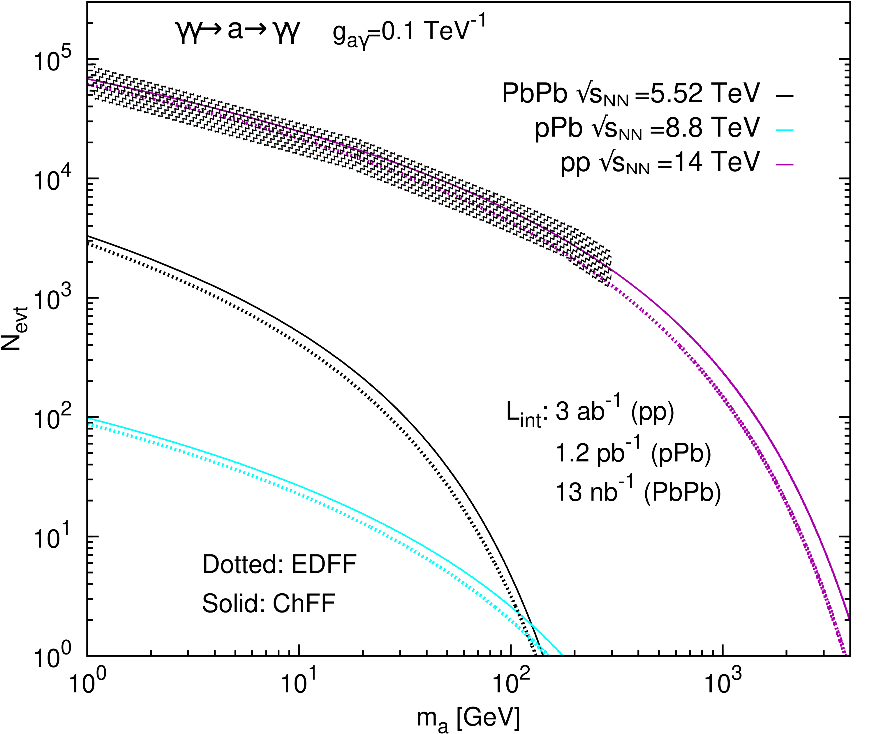
Figure 6: Total number of ALPs events expected via $\gamma\gamma\to a\to\gamma\gamma$ in p-p, p-Pb, and Pb-Pb UPCs at the LHC as a function of ALP mass, for fixed ALP-photon coupling $g_{a\gamma}=0.1~{}\text{TeV}^{-1}$ (approximately corresponding to the current experimental limits over this mass range dEnterria:2021ljz ) computed with EDFF (dotted) and ChFF (solid) $\gamma$ fluxes. The hatched area around the p-p curve indicates the range of masses below $m_{a}\approx 300$ GeV where the detection is hindered due to pileup and lack of proton tagging acceptance.

IV.8 Massive gravitons

The production of spin-2 massive gravitons in UPCs can be also computed with our setup. We consider the effective field theory of a massive graviton $G$ interacting with the photon field, where the kinetic term of $G$ is the well-known Fierz–Pauli Lagrangian with the positive-energy condition $\partial_{\mu}G^{\mu\nu}=0$. The interaction between the $G$ and $\gamma$ is then described by the Lagrangian Das:2016pbk

$$\mathcal{L} \supset -\frac{\kappa_{\gamma}}{\Lambda}T_{\mu\nu}^{\gamma}G^{\mu\nu},$$ (28)

where $T_{\mu\nu}^{\gamma}$ is the energy-momentum tensor of the photon, and $\kappa_{\gamma}/\Lambda$ the effective graviton-photon coupling. The LO decay width is given by $\Gamma_{G\to\gamma\gamma}=\kappa_{\gamma}^{2}m_{G}^{3}/(80\pi\Lambda^{2})$. The number of total events of $\gamma\gamma\to G$ at the LHC are displayed in Fig. 7 for a choice of coupling $\kappa_{\gamma}/\Lambda=1~{}\mathrm{TeV}^{-1}$ in p-p, p-Pb, and Pb-Pb UPCs, as a function of $G$ mass, for the EDFF and ChFF $\gamma$ fluxes. The hatched area around the p-p luminosities indicate that for the range of masses below $m_{G}\approx 300$ GeV, graviton detection is hindered in p-p UPCs due to pileup and lack of proton tagging acceptance. As for ALPs, the plot confirms that Pb-Pb UPCs provide the most competitive means to search for massive gravitons in the region $m_{G}\approx 1$–100 GeV, but that searches with p-p UPCs can eventually reach $m_{G}$ values in the multi-TeV scale, with the full LHC integrated luminosity and forward proton taggers to remove pileup background.

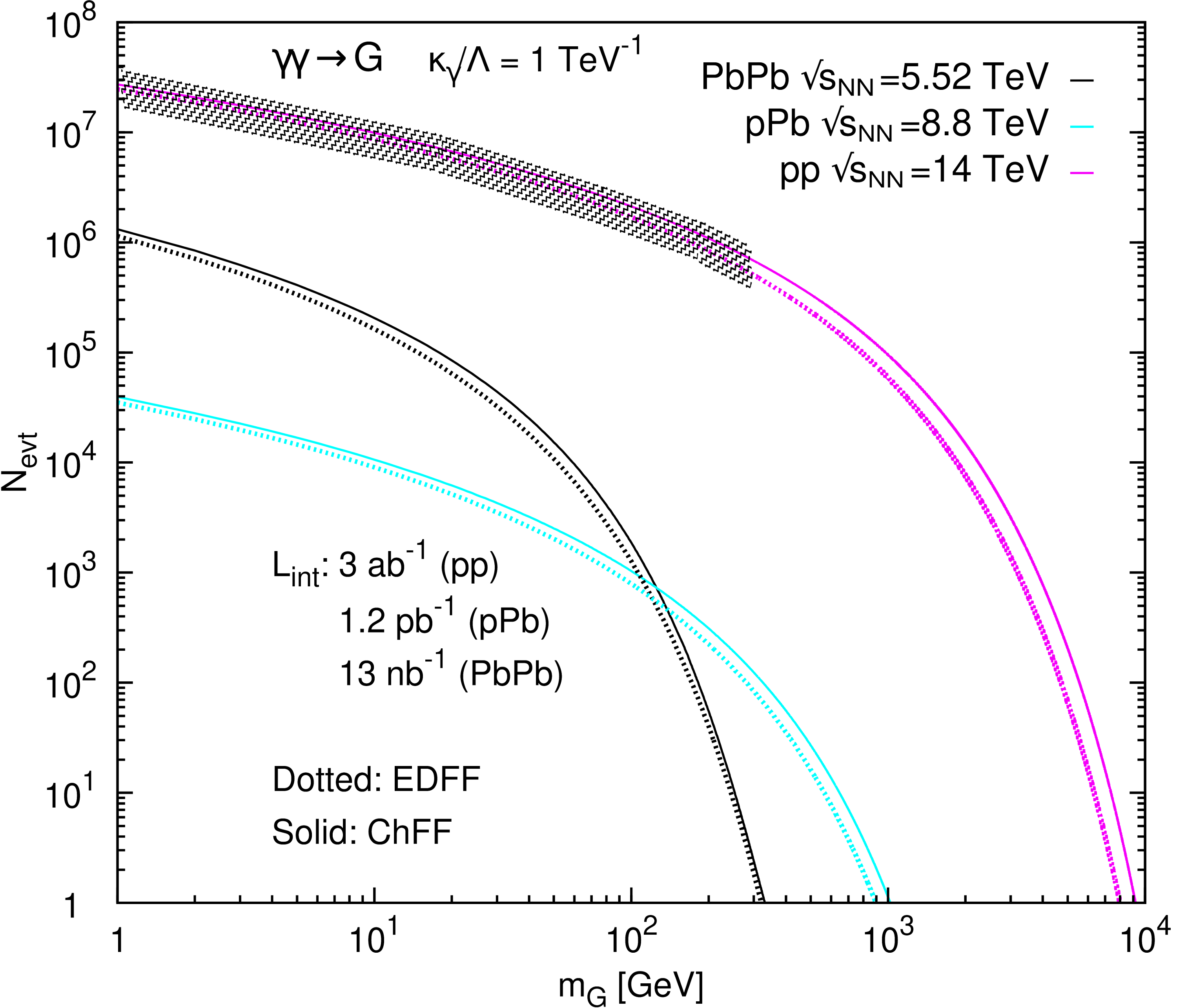
Figure 7: Total number graviton events expected via $\gamma\gamma\to G$ in p-p, p-Pb, and Pb-Pb UPCs at the LHC, as a function of graviton mass, for fixed $\kappa_{\gamma}/\Lambda=1~{}\mathrm{TeV}^{-1}$ graviton-photon coupling computed with EDFF (dotted) and ChFF (solid) $\gamma$ fluxes. The hatched area around the p-p curve indicates the range of masses below $m_{G}\approx 300$ GeV where the detection is hindered due to pileup and lack of proton tagging acceptance.

V Differential photon-photon cross section results: Data vs. gamma-UPC

In this section we present differential cross sections for exclusive dileptons, $\gamma\gamma\to\ell^{+}\ell^{-}$ and light-by-light scattering, $\gamma\gamma\to\gamma\gamma$, in Pb-Pb UPCs at $\sqrt{s_{{}_{\text{NN}}}}=5.02$ TeV where our calculations can be compared to existing LHC data and to alternative predictions from the UPC-dedicated Starlight and Superchic MC generators. In all cases, gamma-UPC results derived with EDFF and ChFF photon fluxes are presented.

V.1 Exclusive dielectrons in Pb-Pb UPCs $\sqrt{s_{{}_{\text{NN}}}}=5.02$ TeV

The exclusive production of electron-positron pairs in photon-photon collisions, $\gamma\gamma\to e^{+}e^{-}$, known as the Breit–Wheeler (B–W) process Breit:1934zz , is the simplest elementary process in two-photon physics. In addition, the B–W continuum constitutes a background for the measurement of multiple dielectron resonances (in particular vector meson ones produced via exclusive photon-hadron collisions), which needs to be properly understood and subtracted. The simplicity and large cross section of the B–W process has facilitated its measurement in hadronic UPCs multiple times (by the WA93 Vane:1992ms , CERES/NA45 CERESNA45:1994cpb , STAR STAR:2004bzo ; STAR:2019wlg , PHENIX PHENIX:2009xtn , CDF CDF:2006apx , ALICE ALICE:2013wjo , CMS CMS:2012cve ; CMS:2018erd ; CMS:2018uvs , and ATLAS ATLAS:2015wnx ; ATLAS:2017fur ; ATLAS:2020mve experiments), and has become a clean final state to test the theoretical ingredients of UPC cross section calculations.

Table 12: Fiducial exclusive dielectron cross sections measured in Pb-Pb UPCs at $\sqrt{s_{{}_{\text{NN}}}}=5.02$ TeV ($E_{\mathrm{T}}^{e}>2$ GeV , $|y^{e}|<2.4$, $m_{e^{+}e^{-}}>5$ GeV, $p_{\mathrm{T},e^{+}e^{-}}<1$ GeV), compared to the theoretical gamma-UPC results obtained with EDFF and ChFF $\gamma$ fluxes (and their average), and to the Starlight and Superchic MC predictions.

Process, system	Scaled CMS data CMS:2018erd	gamma-UPC $\sigma$			Starlight $\sigma$	Superchic $\sigma$
		EDFF	ChFF	average
$\gamma\gamma\to e^{+}e^{-}$, Pb-Pb at 5.02 TeV	$275\pm 55$ $\mu$b	272 $\mu$b	326 $\mu$b	$298\pm 28$ $\mu$b	285 $\mu$b	318 $\mu$b

Table 12 lists the integrated fiducial cross sections, measured by CMS in Pb-Pb UPCs at $\sqrt{s_{{}_{\text{NN}}}}=5.02$ TeV CMS:2018erd compared to our gamma-UPC calculations with the two form factors (and their average), as well as to the Starlight 3.0 Klein:2016yzr and Superchic 3.03 Harland-Lang:2018iur predictions. For comparison purposes, the original CMS experimental uncorrected yields have been scaled to a fully corrected cross section by using their known ratio to the corresponding reconstructed Starlight result over the measured fiducial phase space ($E_{\mathrm{T}}^{e}>2$ GeV , $|y^{e}|<2.4$, $m_{e^{+}e^{-}}>5$ GeV, $p_{\mathrm{T},e^{+}e^{-}}<1$ GeV) CMS:2018erd . The first observation is that the EDFF and Starlight (as well as ChFF and Superchic) results are very similar, and the data seem to fall in between all predictions. In Fig. 8, we plot the B–W differential distributions as a function of dielectron invariant mass (left) and rapidity (right) compared to all theoretical predictions. Within the current experimental uncertainties, all calculations are consistent with the measurement, calling for upcoming higher-precision B–W measurements (e.g. in the higher $m_{e^{+}e^{-}}\gtrsim 8$ GeV mass region which features smaller systematic uncertainties) to be able to better discriminate among the different model ingredients.

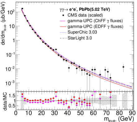
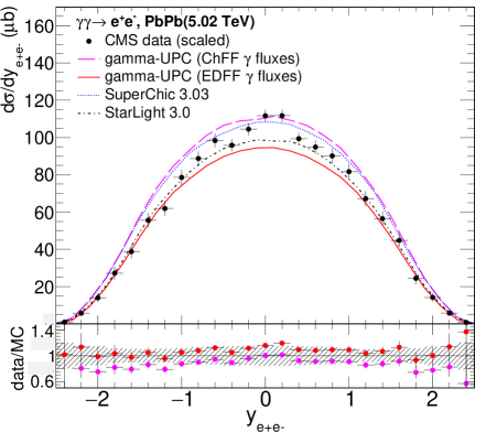
Figure 8: Comparison of the differential fiducial cross sections for exclusive $e^{+}e^{-}$ production in Pb-Pb UPCs at $\sqrt{s_{{}_{\text{NN}}}}=5.02$ TeV as a function of pair invariant mass (left) and rapidity (left) predicted by gamma-UPC (EDFF and ChFF $\gamma$ fluxes), Starlight, and Superchic. The data points show the CMS results CMS:2018erd scaled as explained in the text. The bottom insets show the ratio of the CMS results (with associated systematic uncertainties indicated by hashed boxes) to the EDFF (red) and ChFF (purple) gamma-UPC predictions.

V.2 Exclusive dimuons in Pb-Pb UPCs at $\sqrt{s_{{}_{\text{NN}}}}=5.02$ TeV

Like its dielectron counterpart, the exclusive dimuon production in UPCs is also a clean standard-candle process that can be used to calibrate our theoretical understanding of EPA fluxes, survival probabilities, higher-order QED corrections, etc. At the LHC, the process has been measured with proton CMS:2011vma ; ATLAS:2015wnx ; ATLAS:2017sfe ; CMS:2018uvs ; ATLAS:2020mve and nuclear beams CMS:2020skx ; ATLAS:2020epq , and a detailed discussion of the Superchic and Starlight predictions confronted to the differential ATLAS data has been presented in Harland-Lang:2021ysd . In Table 13, we compare the integrated fiducial cross section measured in Pb-Pb UPCs at $\sqrt{s_{{}_{\text{NN}}}}=5.02$ TeV to the gamma-UPC, Starlight, and Superchic predictions. The results with ChFF flux (and Superchic) seem to overshoot the total fiducial cross section of the ATLAS measurement by 18%, while the EDFF (and Starlight) cross section undershots it by 6%. The ChFF and EDFF average agrees perfectly with the data.

Table 13: Fiducial exclusive dimuon cross sections measured in Pb-Pb UPCs at $\sqrt{s_{{}_{\text{NN}}}}=5.02$ TeV (with $p_{\mathrm{T}}^{\mu}>4$ GeV, $|\eta^{\mu}|<2.4$, $m_{\mu^{+}\mu^{-}}>10$ GeV, $p_{\mathrm{T},\mu^{+}\mu^{-}}<2$ GeV), compared to the theoretical gamma-UPC results obtained with EDFF and ChFF $\gamma$ fluxes (and their average), as well as with the Starlight and Superchic MC predictions.

Process, system	ATLAS data ATLAS:2020epq	gamma-UPC $\sigma$			Starlight $\sigma$	Superchic $\sigma$
		EDFF	ChFF	average
$\gamma\gamma\to\mu^{+}\mu^{-}$, Pb-Pb at 5.02 TeV	$34.1\pm 0.8$ $\mu$b	$32.1$ $\mu$b	$40.4$ $\mu$b	$36.2\pm 4.2$ $\mu$b	$32.1$ $\mu$b	$38.9$ $\mu$b

In Fig. 9, the differential cross sections of exclusive dimuons measured by ATLAS as a function of invariant mass (top), pair rapidity (second row), and cosine of the pair polar angle (third and bottom rows) are plotted in different regions of phase space (from left to right) compared to the corresponding gamma-UPC results with EDFF and ChFF $\gamma$ fluxes, and to these same predictions but normalized (nEDFF and nChFF) to match the measured fiducial cross section. The $\chi^{2}$ goodness-of-fit, determined considering only experimental uncertainties, and number of data points for the rescaled theoretical predictions with respect to the experimental data are listed in each panel. The total $\chi^{2}$ for the overall predictions with nEDFF and nChFF fluxes are respectively $393$ and $327$ for $191$ data points. Namely, the data-theory comparison is slightly better with nChFF than nEDFF fluxes, indicating that the ChFF spectrum provides a better shape agreement with the data. Figure 10 shows the differential exclusive-dimuon cross section as a function of mininum (left) and maximum (right) initial photon energy in data and theory.

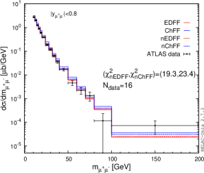
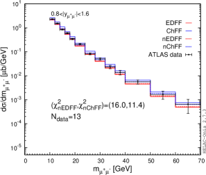
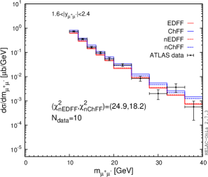
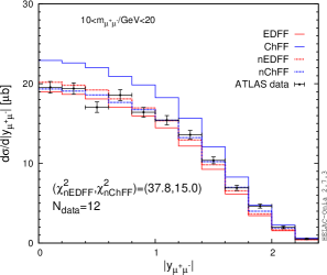
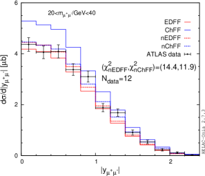
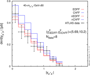
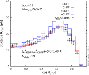
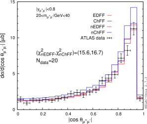
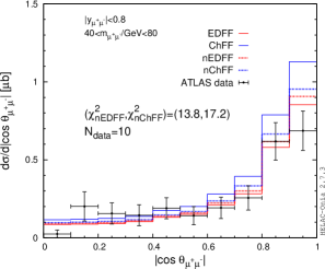
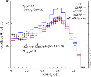
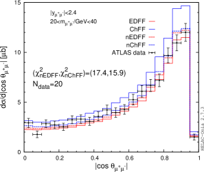
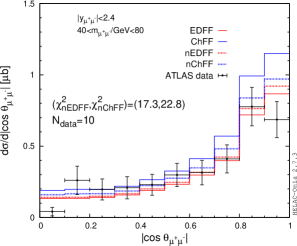
Figure 9: Differential cross section of exclusive dimuon production in Pb-Pb UPCs $\sqrt{s_{{}_{\text{NN}}}}=5.02$ TeV as a function of various kinematic variables in different regions of phase space. The data (black points) ATLAS:2020epq are compared to gamma-UPC predictions (histograms) with EDFF and ChFF fluxes. The dotted histograms, nEDFF and nChFF, have been obtained normalizing the EDFF and ChFF predictions, respectively, to match the measured total fiducial cross section. Data-theory $\chi^{2}$ values are quoted for nEDFF and nChFF fluxes.

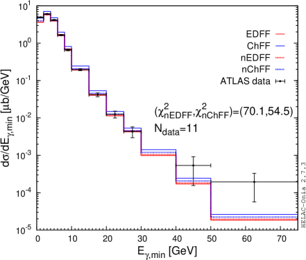
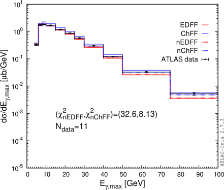
Figure 10: Differential cross section in terms of minimum (left) and maximum (right) initial photon energies in exclusive dimuon production in Pb-Pb UPCs at $\sqrt{s_{{}_{\text{NN}}}}=5.02$ TeV. The data (black points) ATLAS:2020epq are compared to the histograms with the gamma-UPC predictions normalized (nEDFF and nChFF) and not (EDFF and ChFF) to the measured fiducial cross sections. Data-theory $\chi^{2}$ values are quoted for nEDFF and nChFF fluxes

V.3 Light-by-light scattering in Pb-Pb UPCs at $\sqrt{s_{{}_{\text{NN}}}}=5.02$ TeV

The loop-induced LbL signal is generated with gamma-UPC plus MadGraph5_aMC@NLO v2.6.6 Alwall:2014hca ; Hirschi:2015iia with the virtual box contributions computed at leading order. Table 14 compares the integrated fiducial cross sections measured by ATLAS ATLAS:2020hii with the gamma-UPC using EDFF and ChFF $\gamma$ fluxes and the Superchic predictions. The measured cross section is about 2 standard deviations above the gamma-UPC and Superchic predictions.

Table 14: Fiducial light-by-light cross sections measured in Pb-Pb UPCs at $\sqrt{s_{{}_{\text{NN}}}}=5.02$ TeV (with $E_{\mathrm{T}}^{\gamma}>2.5$ GeV , $|\eta^{\gamma}|<2.4$, $m_{\gamma\gamma}>5$ GeV, $p_{\mathrm{T},\gamma\gamma}<1$ GeV), compared to the theoretical gamma-UPC results obtained with EDFF and ChFF $\gamma$ fluxes (and their average), as well as with the Superchic MC prediction.

Process, system	ATLAS data ATLAS:2020hii	gamma-UPC $\sigma$			Superchic $\sigma$
		EDFF	ChFF	average
$\gamma\gamma\to\gamma\gamma$, Pb-Pb at 5.02 TeV	$120\pm 22$ nb	$63$ nb	$76$ nb	$70\pm 7$ nb	$78\pm 8$ nb

In Fig. 11, the differential LbL cross sections measured by ATLAS as a function of invariant mass (top left), single photon $p_{\mathrm{T}}$ (top right), pair rapidity (bottom left), and cosine of the pair polar angle (bottom right) are compared to the corresponding gamma-UPC results with absolute (EDFF and ChFF) and normalized (nEDFF and nChFF) $\gamma$ fluxes. The overall $\chi^{2}$ is $9.58$ and $10.1$ for nEDFF and nChFF fluxes, respectively, with $17$ data points. The data-theory $\chi^{2}$ comparisons are very similar for nChFF and nEDFF fluxes ($\chi^{2}/N_{\text{data}}\approx 0.6$) indicating that both reproduce well the shapes of the LbL distributions measured in data within the relatively large experimental uncertainties. More accurate and precise LbL data are needed in order to understand if the moderate “excess” apparent in the first mass bin ($m_{\gamma\gamma}=5$–10 GeV) with respect to the predictions is real.

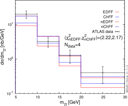
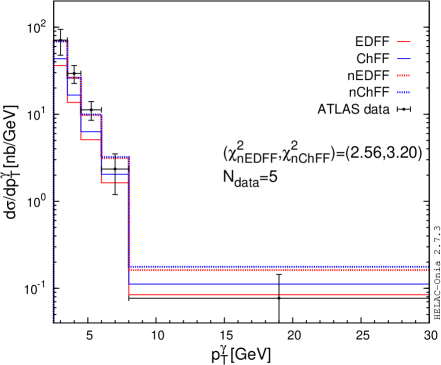
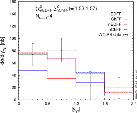
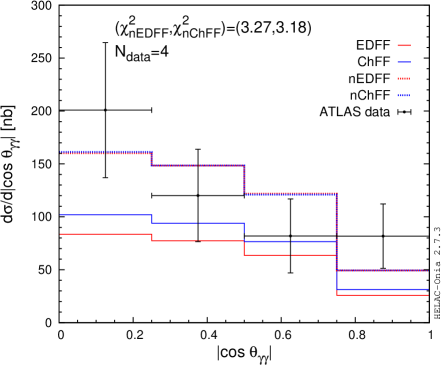
Figure 11: Differential cross sections for light-by-light scattering as a function of various diphoton variables measured in Pb-Pb UPCs at $\sqrt{s_{{}_{\text{NN}}}}=5.02$ TeV (black data points) ATLAS:2020hii compared to our theoretical predictions (red and blue solid-line histograms for EDFF and ChFF, respectively). The dotted histograms (labeled as normalized EDFF and ChFF, nEDFF and nChFF, respectively) are the same predictions rescaled to match the experimental value of the fiducial cross section.

VI gamma-UPC output and upcoming improvements

The first release of the gamma-UPC code contains all the theoretical ingredients described previously in Sections II and III that lead to the results presented in Sections IV and V. Such a code provides the baseline framework to compute the production cross section and event generation of any UPC final state of interest at the LHC and other hadron colliders (RHIC, FCC,…). We provide next a few more details on the gamma-UPC event generation output and ongoing/future developments.

The output of gamma-UPC is not just the photon-fusion fiducial or differential cross sections (in pb units) for the chosen process, but also unweighted MC events are generated in LHE format Alwall:2006yp using the default machinery of the MadGraph5_aMC@NLO and HELAC-Onia codes. The produced LHE output file contains the standard input kinematics and cross section of the generated process in the <init> block, as well as the four-momenta of all produced central particles for each <event>. In the p-p case, since most of the exclusive photon-photon processes are measured at the LHC employing forward proton tagging to get rid of the large pileup background, the gamma-UPC code can also provide as output the 4-momenta kinematics of the two outgoing protons (in the form of a second ancillary LHE file). Such information can then be used to transport the protons, through the beamline magnetic lattice, from the interaction point up to the down- and up-stream taggers in order to determine the experimental acceptance and efficiency of the latter for the physics process in question CMS:2021ncv ; Tasevsky:2015xya .

Further improvements and extensions of gamma-UPC are ongoing or under consideration and will likely be part of a second release of the code, among which:

1. Nonzero photon transverse momentum $\boldsymbol{k_{\perp}}$: Although our ChFF flux, Eq. (16), contains an explicit dependence on the photon $k_{\perp}$ (related to the photon virtuality via $Q^{2}=k_{\perp}^{2}+E_{\gamma}^{2}/\gamma_{\mathrm{L}}^{2}$), our cross sections are fully integrated over the $Q$ and $k_{\perp}$ of the colliding photons, and therefore the centrally produced system $\gamma\gamma\to X$ is produced at rest, $p_{\mathrm{T}}^{X}=0$. As the photon density follows a $1/k_{\perp}^{2}$ dependence and the $k_{\perp}$ values are many orders-of-magnitude smaller than the longitudinal photon energy, the approximation that both photons are real ($Q\approx 0$) has no actual numerical impact on the computed cross sections. In addition, the assumption that the colliding photons have zero $k_{\perp}$, i.e., that the central system is produced exactly at rest, has no real experimental implication either because the detector resolution smears out the energies of the decay products of the central system leading to $p_{\mathrm{T}}^{X}$ values that, though nonzero, are still well below $p_{\mathrm{T}}^{X}\approx 1$ GeV (the usual upper limit imposed in the experimental analyses to remove nonexclusive backgrounds). Nonetheless, as discussed in the introduction, in reality the colliding photons can have very small but nonzero virtualities up to about $Q^{2}<1/R^{2}\approx~{}0.08$ GeV² for protons and $Q^{2}<10^{-3}$ GeV² for Pb nuclei, and the next release of the code will include the impact of this small (few tens or hundred MeV) extra photon $k_{\perp}$ in the MC event generator output.

2. Semiexclusive photon-photon processes: Our calculations use the elastic $\gamma$ fluxes for both hadrons, but $\gamma\gamma$ collisions can also occur in semielastic processes where one of the photons is emitted from the constituents (partons or nucleons in p-p or A-A UPCs, respectively) of one of the hadrons leading to its breakup. Although the cross sections for such semiexclusive collisions are suppressed compared to the fully coherent cases (e.g. they scale at most as $Z^{3}$ compared to the $Z^{4}$ dependence of the A-A UPCs case), they can constitute a background to the elastic cross sections in the absence of detectors at very forward angles (Roman Pots and Zero Degree Calorimeters for p-p and A-A UPCs, respectively) that can be used to veto activity from the hadronic breakup. Our setup can be easily extended to incorporate semiexclusive collisions of inelastic photons from the hadron constituents, on the one hand, with elastic photons from the other intervening hadron, on the other.

3. NLO QED and weak corrections: The availability of full NLO corrections accounting for virtual and real QED and weak emissions is a requirement for accurate and precise calculations of photon-photon cross sections. In particular when comparing the data to theory to extract precision SM parameters (such as e.g. the $g-2$ of the tau lepton via $\gamma\gamma\to\tau^{+}\tau^{-}$ delAguila:1991rm ; Atag:2010ja ; Beresford:2019gww ; Dyndal:2020yen ) and/or to search for absolute or differential cross section deviations from the SM prediction due to new physics contributions. Theoretical developments in this direction are already part of MadGraph5_aMC@NLO Frederix:2018nkq and need to be properly interfaced with the gamma-UPC setup to account for the particularities of photon-photon collisions.

4. Electroweak boson fusion processes with elastic photons: Photon-photon collisions are actually a fraction of the multiple combinations of fusion processes among electroweak vector bosons (W, Z, and $\gamma$). Interesting possibilities exist if one considers semiexclusive photon-V collisions where the photon is radiated coherently from one hadron, and the weak boson V = W or Z is emitted from the constituent partons of the other. Such “hybrid” photon-W collisions at hadron colliders have been considered in the literature Alva:2014gxa and can be also in principle incorporated into our gamma-UPC setup by combining the equivalent W flux (the effective W/Z fluxes from leptons have been implemented in MG5_aMC recently Ruiz:2021tdt ) or Z flux (for loop-induced $\gamma-Z$ fusion) from one hadron with the coherent photon of the other hadron.

5. UPCs in electron-proton,nucleus collisions: The photon flux of an electron has larger virtualities than that of a hadron beam, but photon-photon collisions have been studied at electron-proton colliders for a long time Vermaseren:1982cz ; Schuler:1997ex . The planned Electron-Ion-Collider (EIC) AbdulKhalek:2021gbh will allow for the first time to study $\gamma\gamma$ collisions issuing from the fusion of $e^{\pm}$ and heavy-ion photon fluxes, providing novel opportunities for studies of interest Chwastowski:2022fzk ; Davoudiasl:2021mjy . The extension of gamma-UPC to handle and combine the incoming fluxes of photons from electrons and protons or heavy-ions is also under consideration to facilitate the preparation of EIC feasibility studies.

6. Forward neutron emission: The exclusive photon-photon fusion cross sections calculated with gamma-UPC are fully inclusive with respect to any additional potential electromagnetic soft excitation(s) of the colliding nuclei (which in principle completely factorize from the photon-photon fusion process itself), and which may lead to later-time nuclear deexcitations with very forward neutron emission. For this reason, the data–theory comparisons shown in Figs. 8– 11 are fully inclusive in forward neutron topology. However, one of the main advantages of generating $\gamma\gamma$ collisions with the dedicated Starlight MC code is the possibility of calculating cross sections for UPCs with ions including or vetoing the concurrent emission of $Xn$ (with $X=0,1,\cdots$) forward neutrons from one or both interacting ions. Events with neutron multiplicity indicate the presence of mutual e.m. excitation of the passing-by ions, or their nuclear breakup. Experimentally, such neutrons are usually detected in Zero Degree Calorimeters (ZDCs) ALICE:1999edx ; Adler:2000bd ; Grachov:2006ke ; White:2010zzd and their veto helps to reduce nonexclusive backgrounds. A dedicated stand-alone MC code exists, called nOOn, for the calculation of forward neutron emission in UPCs with heavy ions Broz:2019kpl that can be eventually combined with the gamma-UPC setup.

These upcoming expected improvements will be reported in the gamma-UPC code version information at the http://cern.ch/hshao/gammaupc.html webpage.

VII Summary

We have presented a new phenomenological code development that is able of automatically generating arbitrary photon-photon collision events in ultraperipheral collisions (UPCs) of protons and heavy ions, A  B $\xrightarrow{\gamma\gamma}$ A  $X$  B, at high energies. Two types of elastic photon fluxes, as well as associated survival probabilities of the photon-emitting hadrons, have been implemented into the MadGraph5_aMC@NLO and HELAC-Onia codes, based on the electric-dipole (EDFF) and charge (ChFF) form factors for proton and light and heavy nuclei. This setup, named gamma-UPC (downloadable from http://cern.ch/hshao/gammaupc.html), can compute the cross sections and generate any exclusive final state of interest producing SM (in particular quarkonia) and BSM particles in UPCs at high energies, including higher-order real corrections for processes with extra photons and/or gluons emitted. From the differences found between the EDFF- and ChFF-based results, theoretical uncertainties in the cross sections linked to the elastic $\gamma$ spectrum and hadron survival probabilities for $\gamma\gamma\to X$ processes at low ($m_{X}\approx 10$ GeV) and high ($m_{X}\approx 100$ GeV) masses are estimated to vary over 12–25% for Pb-Pb, 7–15% for p-Pb, and 6–12% for p-p UPCs. Such uncertainties can nonetheless be significantly reduced by taking ratios of two exclusive $\gamma\gamma$ cross sections (e.g. by using exclusive dimuon production as a reference baseline process in the denominator) at the same photon-photon c.m. energy $W_{\gamma\gamma}$.

Illustrative examples of $\gamma\gamma$ cross sections computed with this setup have been shown for proton-proton, proton-nucleus, and nucleus-nucleus UPCs at the Large Hadron Collider (LHC) and Future Circular Collider (FCC). Total photon-fusion cross sections for the exclusive production of spin-0, 2 resonances (four charmonium states, four bottomonium states, paraditauonium, and the Higgs boson), as well as for pairs of SM particles ($\mathrm{J}/\psi\mathrm{J}/\psi$, WW, ZZ, Z$\gamma$, $t\overline{t}$, HH) and for BSM particles (axionlike and massive gravitons) have been presented. All such processes provide valuable novel SM tests ($\tau$ and top-quark electromagnetic moments, quartic gauge couplings, properties of QCD and QED bound states, etc.) and unique BSM searches. Differential cross sections for the production of exclusive dielectrons, dimuons, and light-by-light scattering have been compared to existing LHC Pb-Pb data as well as to predictions from other UPC-dedicated MC models such as Starlight and Superchic. These more detailed comparisons indicate that, for the processes implemented in the two latter MC codes, the gamma-UPC EDFF and ChFF results are, respectively, very consistent with the Starlight and Superchic ones (and can be, therefore, used as “proxies” of the latter whenever the physics process is not available in them).

Ongoing and upcoming developments that will extend the gamma-UPC features (semiexclusive collisions, weak-boson fusion processes, UPCs in e-p,A, etc.) have been also outlined. This code provides a novel useful tool for carrying out studies of any arbitrary final state produced in photon-photon collision at hadron colliders, providing not only the cross section calculation and automatic generation of events for any SM/BSM signal of interest, but also of any potential associated backgrounds. The upcoming incorporation of full electroweak corrections at next-to-leading-order accuracy and beyond in MadGraph5_aMC@NLO will allow for a reduction of theoretical uncertainties and the possibility of carrying out more precise SM tests, and BSM searches, with exclusive photon-photon processes employing our setup.

Acknowledgments.—

Support from the European Union’s Horizon 2020 research and innovation program (grant agreement No.824093, STRONG-2020, EU Virtual Access “NLOAccess”), the French ANR (grant ANR-20-CE31-0015, “PrecisOnium”), and the CNRS IEA (grant No.205210, “GlueGraph"), are acknowledged.

Appendix A Basic code instructions

The gamma-UPC code is written in Fortran90. A brief set of instructions on how to compile and run gamma-UPC stand-alone, or with MadGraph5_aMC@NLO or HELAC-Onia are provided below. More technical details can be found at http://cern.ch/hshao/gammaupc.html, where the code can be downloaded.

A.1 Standalone usage

The gamma-UPC can be run stand-alone. This package contains a module, test.f90, which acts as the driver when working in this mode. The code is compiled with the usual shell command

⬇

> make test

We assume a gfortran compiler. The test program embedded in test.f90 can be run by executing:

⬇

> ./test

If one just compiles the code via

⬇

> make

a static library libgammaUPC.a will be generated. The gamma-UPC subroutines can be accessed by including the Fortran90 module via

⬇

USE ElasticPhotonPhotonFlux

The common parameters of defining the two beams can be found in run90.inc via

⬇

INCLUDE ‘run90.inc‘

The energies per nucleon of the two beams are ebeam(1) and ebeam(2) in units of GeV, while the nuclear mass and charge numbers of the first (second) beam are defined via the integers nuclearA_beam1 (nuclearA_beam2) and nuclearZ_beam1 (nuclearZ_beam2), respectively. The value of $\alpha$ can be changed from its default of $1/137$ by assigning alphaem_elasticphoton a new value. The bool flag USE_CHARGEFORMFACTOR4PHOTON is used to select EDFF (.FALSE.) or ChFF (.TRUE.) $\gamma$ fluxes. After the above preparation, one can call the function dLgammagammadW_UPC to obtain the effective two-photon luminosity at a given resonance mass m, i.e. $\frac{d{\mathcal{L}}^{(\mathrm{A\,B})}_{\gamma\gamma}}{dW_{\gamma\gamma}}\big{|}_{W_{\gamma\gamma}=m}$, as follows:

⬇

dLdW=dLgammagammadW_UPC(m,icoll,1)

where the icoll$=1,2,3$ argument applies to p-p, p-A, A-B collisions, respectively. The two-photon differential distribution normalized by $(x_{1}x_{2})$, i.e., $\frac{1}{x_{1}x_{2}}\frac{\mathrm{d}^{2}N^{(\mathrm{AB})}_{\gamma_{1}/\mathrm{Z}_{1},\gamma_{2}/\mathrm{Z}_{2}}}{\mathrm{d}E_{\gamma_{1}}\mathrm{d}E_{\gamma_{2}}}$ can be accessed via

⬇

dNpp=PhotonPhotonFlux_pp(x1,x2)

dNpA=PhotonPhotonFlux_pA_WoodsSaxon(x1,x2)

dNAB=PhotonPhotonFlux_AB_WoodsSaxon(x1,x2)

for p-p, p-A, A-B collisions respectively, where x1 and x2 are the fractions $x_{1}$ and $x_{2}$ of the hadron energy carried out by the photons, for the two incoming beams. The initialization for generating grids in the first call may take a few minutes. However, the numerical evaluations should be fast enough and suitable for the numerical phase space integrations as long as the grids have been successfully produced.

A.2 Usage of gamma-UPC in HELAC-Onia

The program gamma-UPC has been integrated into HELAC-Onia Shao:2012iz ; Shao:2015vga for the exclusive two-photon production of quarkonia bound states, and easily extendable to any spin-even resonance by introducing a “fake” $q\overline{q}$ state with any arbitrary mass and diphoton width, as e.g. done for ditauonium dEnterria:2022ysg . A few parameters need to be specified before launching the jobs, as follows:

⬇

HO> set colpar = 14

HO> set nuclearA_beam1 = <an integer>

HO> set nuclearA_beam2 = <an integer>

HO> set nuclearZ_beam1 = <an integer>

HO> set nuclearZ_beam2 = <an integer>

HO> set UPC_photon_flux_type = <an integer between 1 to 6>

where the nuclearA_beam1 (nuclearA_beam2) and nuclearZ_beam1 (nuclearZ_beam2) integers are nuclear mass and atomic numbers for the first (second) beam, respectively. The parameter UPC_photon_flux_type determines the usage of the UPC photon-photon fluxes as explained in input/default.inp. Namely, setting UPC_photon_flux_type=$1,6$ selects EDFF and ChFF fluxes, respectively, with their corresponding hadronic-nonoverlap requirement. In such a case, the two initial particles must be photons. The parameters energy_beam1 and energy_beam2 (in GeV/nucleon) are interpreted as the energy of the beams per nucleon.

A.3 Usage of gamma-UPC in MadGraph5_aMC@NLO

One can also directly call gamma-UPC within MadGraph5_aMC@NLO Alwall:2014hca for the exclusive two-photon production of any SM or BSM final state. The two initial particles of the generated process must be two photons. In order to call gamma-UPC, one needs to specify the following parameters in run_card.dat, taking here p-Pb UPCs at $\sqrt{s_{\rm NN}}=8.16$ TeV as an example:

#*********************************************************************
# Collider type and energy                                           *
# lpp: 0=No PDF, 1=proton, -1=antiproton,                            *
#                2=elastic photon of proton/ion beam                 *
#             +/-3=PDF of electron/positron beam                     *
#             +/-4=PDF of muon/antimuon beam                         *
#*********************************************************************
  2     = lpp1 ! beam 1 type
  2     = lpp2 ! beam 2 type
  7000.0        = ebeam1 ! beam 1 total energy in GeV
  574080.0      = ebeam2 ! beam 2 total energy in GeV

#*********************************************************************
# PDF CHOICE: this automatically fixes alpha_s and its evol.         *
# pdlabel: lhapdf=LHAPDF (installation needed) [1412.7420]           *
#          iww=Improved Weizsaecker-Williams Approx.[hep-ph/9310350] *
#          eva=Effective W/Z/A Approx.       [2111.02442]            *
#          edff=EDFF in gamma-UPC            [2207.03012]            *
#          chff=ChFF in gamma-UPC            [2207.03012]            *
#          none=No PDF, same as lhapdf with lppx=0                   *
#*********************************************************************
  edff  = pdlabel ! PDF set

#*********************************************************************
# Heavy ion PDF / rescaling of PDF                                   *
#*********************************************************************
  1    = nb_proton1 # number of protons for the first beam
  0    = nb_neutron1 # number of neutrons for the first beam
  82   = nb_proton2 # number of protons for the second beam
  126  = nb_neutron2 # number of neutrons for the second beam

Note that unlike the previous two cases (running stand-alone and with HELAC-Onia), the energy of the ion beam is its total energy (namely, $A\times E_{\mathrm{beam}}$, where $A=Z+N$ is the sum of the number of protons and neutrons, i.e., the total number of nucleons) instead of the energy per nucleon. The two beam types (lpp1,lpp2) must be chosen as $2$, and pdlabel can be either iww [cf. Eq. (2)], edff (EDFF), or chff (ChFF) elastic photon fluxes. Note that the iww choice is not applicable for ion beams, but only for protons. The parameters nb_proton$i$ and nb_neutron$i$ set the numbers of protons and neutrons, respectively, in the $i$th beam. These are hidden parameters in run_card.dat, which can be explicitly shown by using the prompt command ‘update ion_pdf’ when editing the cards.

References

- (1) C. F. von Weizsäcker, “Radiation emitted in collisions of very fast electrons,” Z. Phys. 88 (1934) 612.
- (2) E. J. Williams, “Nature of the high-energy particles of penetrating radiation and status of ionization and radiation formulae,” Phys. Rev. 45 (1934) 729.
- (3) S. J. Brodsky, T. Kinoshita, and H. Terazawa, “Two Photon Mechanism of Particle Production by High-Energy Colliding Beams,” Phys. Rev. D 4 (1971) 1532.
- (4) V. M. Budnev, I. F. Ginzburg, G. V. Meledin, and V. G. Serbo, “The Two photon particle production mechanism. Physical problems. Applications. Equivalent photon approximation,” Phys. Rept. 15 (1975) 181.
- (5) J. A. M. Vermaseren, “Two Photon Processes at Very High-Energies,” Nucl. Phys. B 229 (1983) 347.
- (6) G. A. Schuler, “Two photon physics with GALUGA 2.0,” Comput. Phys. Commun. 108 (1998) 279, arXiv:hep-ph/9710506.
- (7) S. Uehara, “TREPS: A Monte-Carlo Event Generator for Two-photon Processes at Colliders using an Equivalent Photon Approximation,” arXiv:1310.0157 [hep-ph].
- (8) C. A. Bertulani, S. R. Klein, and J. Nystrand, “Physics of ultra-peripheral nuclear collisions,” Ann. Rev. Nucl. Part. Sci. 55 (2005) 271, arXiv:nucl-ex/0502005.
- (9) A. J. Baltz, “The physics of ultraperipheral collisions at the LHC,” Phys. Rept. 458 (2008) 1, arXiv:0706.3356 [nucl-ex].
- (10) D. d’Enterria, M. Klasen, and K. Piotrzkowski, “High-Energy Photon Collisions at the LHC,” Nucl. Phys. B Proc. Suppl. 179 (2008) 1.
- (11) J. de Favereau de Jeneret, V. Lemaitre, Y. Liu, S. Ovyn, T. Pierzchala, K. Piotrzkowski, X. Rouby, N. Schul, and M. Vander Donckt, “High energy photon interactions at the LHC,” arXiv:0908.2020 [hep-ph].
- (12) ATLAS Collaboration, M. Aaboud et al., “Evidence for light-by-light scattering in heavy-ion collisions with the ATLAS detector at the LHC,” Nature Phys. 13 (2017) 852, arXiv:1702.01625 [hep-ex].
- (13) CMS Collaboration, A. M. Sirunyan et al., “Evidence for light-by-light scattering and searches for axion-like particles in ultraperipheral PbPb collisions at TeV,” Phys. Lett. B 797 (2019) 134826, arXiv:1810.04602 [hep-ex].
- (14) ATLAS Collaboration, G. Aad et al., “Observation of light-by-light scattering in ultraperipheral Pb+Pb collisions with the ATLAS detector,” Phys. Rev. Lett. 123 (2019) 052001, arXiv:1904.03536 [hep-ex].
- (15) ATLAS Collaboration, G. Aad et al., “Measurement of light-by-light scattering and search for axion-like particles with 2.2 nb-1 of Pb+Pb data with the ATLAS detector,” JHEP 11 (2021) 050, arXiv:2008.05355 [hep-ex].
- (16) ATLAS Collaboration, G. Aad et al., “Measurement of exclusive production in proton-proton collisions at TeV with the ATLAS detector,” Phys. Lett. B 749 (2015) 242, arXiv:1506.07098 [hep-ex].
- (17) ATLAS Collaboration, M. Aaboud et al., “Measurement of the exclusive process in proton-proton collisions at TeV with the ATLAS detector,” Phys. Lett. B 777 (2018) 303, arXiv:1708.04053 [hep-ex].
- (18) CMS, TOTEM Collaboration, A. M. Sirunyan et al., “Observation of proton-tagged, central (semi)exclusive production of high-mass lepton pairs in pp collisions at 13 TeV with the CMS-TOTEM precision proton spectrometer,” JHEP 07 (2018) 153, arXiv:1803.04496 [hep-ex].
- (19) ATLAS Collaboration, G. Aad et al., “Exclusive dimuon production in ultraperipheral Pb+Pb collisions at TeV with ATLAS,” Phys. Rev. C 104 (2021) 024906, arXiv:2011.12211 [nucl-ex].
- (20) ATLAS Collaboration, “Observation of the process in Pb+Pb collisions and constraints on the -lepton anomalous magnetic moment with the ATLAS detector,” arXiv:2204.13478 [hep-ex].
- (21) CMS Collaboration, “Observation of lepton pair production in ultraperipheral lead-lead collisions at TeV,” arXiv:2206.05192 [nucl-ex].
- (22) CMS Collaboration, S. Chatrchyan et al., “Study of exclusive two-photon production of in pp collisions at TeV and constraints on anomalous quartic gauge couplings,” JHEP 07 (2013) 116, arXiv:1305.5596 [hep-ex].
- (23) CMS Collaboration, V. Khachatryan et al., “Evidence for exclusive production and constraints on anomalous quartic gauge couplings in pp collisions at and 8 TeV,” JHEP 08 (2016) 119, arXiv:1604.04464 [hep-ex].
- (24) ATLAS Collaboration, M. Aaboud et al., “Measurement of exclusive production and search for exclusive Higgs boson production in pp collisions at TeV using the ATLAS detector,” Phys. Rev. D 94 (2016) 032011, arXiv:1607.03745 [hep-ex].
- (25) D. d’Enterria and G. G. da Silveira, “Observing light-by-light scattering at the Large Hadron Collider,” Phys. Rev. Lett. 111 (2013) 080405, arXiv:1305.7142 [hep-ph]. [Erratum: Phys. Rev. Lett. 116 (2016) 129901].
- (26) T. Pierzchala and K. Piotrzkowski, “Sensitivity to anomalous quartic gauge couplings in photon-photon interactions at the LHC,” Nucl. Phys. B Proc. Suppl. 179-180 (2008) 257, arXiv:0807.1121 [hep-ph].
- (27) S. Knapen, T. Lin, H. K. Lou, and T. Melia, “Searching for Axionlike Particles with Ultraperipheral Heavy-Ion Collisions,” Phys. Rev. Lett. 118 (2017) 171801, arXiv:1607.06083 [hep-ph].
- (28) J. Ellis, N. E. Mavromatos, and T. You, “Light-by-Light Scattering Constraint on Born-Infeld Theory,” Phys. Rev. Lett. 118 (2017) 261802, arXiv:1703.08450 [hep-ph].
- (29) F. del Aguila, F. Cornet, and J. I. Illana, “The Possibility of using a large heavy ion collider for measuring the electromagnetic properties of the tau-lepton,” Phys. Lett. B 271 (1991) 256.
- (30) S. Atag and A. A. Billur, “Possibility of Determining Lepton Electromagnetic Moments in Process at the CERN-LHC,” JHEP 11 (2010) 060, arXiv:1005.2841 [hep-ph].
- (31) L. Beresford and J. Liu, “New physics and tau using LHC heavy ion collisions,” Phys. Rev. D 102 (2020) 113008, arXiv:1908.05180 [hep-ph].
- (32) M. Dyndal, M. Klusek-Gawenda, M. Schott, and A. Szczurek, “Anomalous electromagnetic moments of lepton in reaction in Pb+Pb collisions at the LHC,” Phys. Lett. B 809 (2020) 135682, arXiv:2002.05503 [hep-ph].
- (33) R. Bruce et al., “New physics searches with heavy-ion collisions at the CERN Large Hadron Collider,” J. Phys. G 47 (2020) 060501, arXiv:1812.07688 [hep-ph].
- (34) S. Klein et al., “New opportunities at the photon energy frontier,” arXiv:2009.03838 [hep-ph].
- (35) D. d’Enterria et al., “Opportunities for new physics searches with heavy ions at colliders,” in 2022 Snowmass Summer Study. (Mar. 2022). arXiv:2203.05939 [hep-ph].
- (36) R. Horvat, D. Latas, J. Trampetić, and J. You, “Light-by-Light Scattering and Spacetime Noncommutativity,” Phys. Rev. D 101 (2020) 095035, arXiv:2002.01829 [hep-ph].
- (37) S. Atag, S. C. Inan, and I. Sahin, “Extra dimensions in process at the CERN-LHC,” JHEP 09 (2010) 042, arXiv:1005.4792 [hep-ph].
- (38) D. d’Enterria and H.-S. Shao, “Observing true tauonium via two-photon fusion at e+e- and hadron colliders,” Phys. Rev. D 105 (2022) 093008, arXiv:2202.02316 [hep-ph].
- (39) D. d’Enterria, R. Perez-Ramos, and H.-S. Shao, “Ditauonium spectroscopy,” arXiv:2204.07269 [hep-ph].
- (40) G.-M. Yu, Y.-C. Yu, Y.-D. Li, and J.-S. Wang, “Charmonium production in ultra-peripheral heavy ion collisions with two-photon processes,” Nucl. Phys. B 917 (2017) 234, arXiv:1703.06620 [hep-ph].
- (41) E. Chapon et al., “Prospects for quarkonium studies at the high-luminosity LHC,” Prog. Part. Nucl. Phys. 122 (2022) 103906, arXiv:2012.14161 [hep-ph].
- (42) V. P. Gonçalves and B. D. Moreira, “Fully-heavy tetraquark production by interactions in hadronic collisions at the LHC,” Phys. Lett. B 816 (2021) 136249, arXiv:2101.03798 [hep-ph].
- (43) J. Kwiecinski and L. Motyka, “Diffractive production in high-energy collisions as a probe of the QCD pomeron,” Phys. Lett. B 438 (1998) 203, arXiv:hep-ph/9806260.
- (44) J. Kwiecinski, L. Motyka, and A. De Roeck, “The QCD pomeron at TESLA: Motivation and exclusive production,” in 2nd Workshop of the 2nd Joint ECFA / DESY Study on Physics and Detectors for a Linear Electron Positron Collider, p. 556. 10, 1999. arXiv:hep-ph/0001180.
- (45) V. L. Chernyak and S. I. Eidelman, “Hard exclusive two photon processes in QCD,” Prog. Part. Nucl. Phys. 80 (2015) 1, arXiv:1409.3348 [hep-ph].
- (46) V. P. Goncalves, B. D. Moreira, and F. S. Navarra, “Double vector meson production in interactions at hadronic colliders,” Eur. Phys. J. C 76 (2016) 103, arXiv:1512.07482 [hep-ph].
- (47) E. Chapon, C. Royon, and O. Kepka, “Anomalous quartic W W, ZZ, and trilinear WW couplings in two-photon processes at high luminosity at the LHC,” Phys. Rev. D 81 (2010) 074003, arXiv:0912.5161 [hep-ph].
- (48) C. Baldenegro, S. Fichet, G. von Gersdorff, and C. Royon, “Probing the anomalous Z coupling at the LHC with proton tagging,” JHEP 06 (2017) 142, arXiv:1703.10600 [hep-ph].
- (49) D. d’Enterria and J.-P. Lansberg, “Study of Higgs boson production and its decay in processes in proton-nucleus collisions at the LHC,” Phys. Rev. D 81 (2010) 014004, arXiv:0909.3047 [hep-ph].
- (50) D. d’Enterria, D. E. Martins, and P. Rebello Teles, “Higgs boson production in interactions with proton, light-ion, and heavy-ion beams at current and future colliders,” Phys. Rev. D 101 (2020) 033009, arXiv:1904.11936 [hep-ph].
- (51) R. Belusevic and G. Jikia, “Higgs selfcoupling in collisions,” Phys. Rev. D 70 (2004) 073017, arXiv:hep-ph/0403303.
- (52) L. Beresford and J. Liu, “Search Strategy for Sleptons and Dark Matter Using the LHC as a Photon Collider,” Phys. Rev. Lett. 123 (2019) 141801, arXiv:1811.06465 [hep-ph].
- (53) L. Harland-Lang, V. Khoze, M. Ryskin, and M. Tasevsky, “LHC Searches for Dark Matter in Compressed Mass Scenarios: Challenges in the Forward Proton Mode,” JHEP 04 (2019) 010, arXiv:1812.04886 [hep-ph].
- (54) S. Godunov, V. Novikov, A. Rozanov, M. Vysotsky, and E. Zhemchugov, “Quasistable charginos in ultraperipheral proton-proton collisions at the LHC,” JHEP 01 (2020) 143, arXiv:1906.08568 [hep-ph].
- (55) K. Babu and S. Jana, “Probing Doubly Charged Higgs Bosons at the LHC through Photon Initiated Processes,” Phys. Rev. D 95 (2017) 055020, arXiv:1612.09224 [hep-ph].
- (56) V. P. Goncalves, D. E. Martins, and M. S. Rangel, “Searching for axionlike particles with low masses in pPb and PbPb collisions,” Eur. Phys. J. C 81 (2021) 522, arXiv:2103.01862 [hep-ph].
- (57) S. M. Lietti and C. G. Roldao, “Radion and Higgs signals in peripheral heavy ion collisions at the LHC,” Phys. Lett. B 540 (2002) 252, arXiv:hep-ph/0205256.
- (58) Y. Kurochkin, I. Satsunkevich, D. Shoukavy, N. Rusakovich, and Y. Kulchitsky, “On production of magnetic monopoles via fusion at high energy p p collisions,” Mod. Phys. Lett. A 21 (2006) 2873.
- (59) T. Dougall and S. D. Wick, “Dirac magnetic monopole production from photon fusion in proton collisions,” Eur. Phys. J. A 39 (2009) 213, arXiv:0706.1042 [hep-ph].
- (60) S. Baines, N. E. Mavromatos, V. A. Mitsou, J. L. Pinfold, and A. Santra, “Monopole production via photon fusion and Drell–Yan processes: MadGraph implementation and perturbativity via velocity-dependent coupling and magnetic moment as novel features,” Eur. Phys. J. C 78 (2018) 966, arXiv:1808.08942 [hep-ph]. [Erratum: EPJC 79 (2019) 166].
- (61) MoEDAL Collaboration, B. Acharya et al., “Magnetic Monopole Search with the Full MoEDAL Trapping Detector in 13 TeV pp Collisions Interpreted in Photon-Fusion and Drell-Yan Production,” Phys. Rev. Lett. 123 (2019) 021802, arXiv:1903.08491 [hep-ex].
- (62) D. Atwood, S. Bar-Shalom, and A. Soni, “Graviton production by two photon processes in Kaluza-Klein theories with large extra dimensions,” arXiv:hep-ph/9903538.
- (63) Y.-J. Zhou, W.-G. Ma, L. Han, and R.-Y. Zhang, “Associated production of graviton with pair via photon-photon collisions at a linear collider,” Phys. Rev. D 76 (2007) 054003, arXiv:0708.1195 [hep-ph].
- (64) S. C. Inan, “Direct Graviton Production via Photon-Photon Fusion at the CERN-LHC,” Chin. Phys. Lett. 29 (2012) 031301.
- (65) M. W. Krasny, A. Petrenko, and W. Płaczek, “High-luminosity Large Hadron Collider with laser-cooled isoscalar ion beams,” Prog. Part. Nucl. Phys. 114 (2020) 103792, arXiv:2003.11407 [physics.acc-ph].
- (66) CMS Collaboration, “The CMS Precision Proton Spectrometer at the HL-LHC – Expression of Interest,” arXiv:2103.02752 [physics.ins-det].
- (67) ATLAS Collaboration, M. Taševský, “Status of the AFP project in the ATLAS experiment,” AIP Conf. Proc. 1654 (2015) 090001.
- (68) FP420 R&D Collaboration, M. G. Albrow et al., “The FP420 R&D Project: Higgs and New Physics with forward protons at the LHC,” JINST 4 (2009) T10001, arXiv:0806.0302 [hep-ex].
- (69) FCC Collaboration, A. Abada et al., “FCC-hh: The Hadron Collider: Future Circular Collider Conceptual Design Report Volume 3,” Eur. Phys. J. ST 228 (2019) 755.
- (70) A. Dainese et al., “Heavy ions at the Future Circular Collider,” arXiv:1605.01389 [hep-ph].
- (71) S. R. Klein, J. Nystrand, J. Seger, Y. Gorbunov, and J. Butterworth, “STARlight: A Monte Carlo simulation program for ultra-peripheral collisions of relativistic ions,” Comput. Phys. Commun. 212 (2017) 258, arXiv:1607.03838 [hep-ph].
- (72) L. A. Harland-Lang, M. Tasevsky, V. A. Khoze, and M. G. Ryskin, “A new approach to modelling elastic and inelastic photon-initiated production at the LHC: SuperChic 4,” Eur. Phys. J. C 80 (2020) 925, arXiv:2007.12704 [hep-ph].
- (73) M. Boonekamp, A. Dechambre, V. Juranek, O. Kepka, M. Rangel, C. Royon, and R. Staszewski, “FPMC: A Generator for forward physics,” arXiv:1102.2531 [hep-ph].
- (74) J. Alwall, M. Herquet, F. Maltoni, O. Mattelaer, and T. Stelzer, “MadGraph 5 : Going Beyond,” JHEP 06 (2011) 128, arXiv:1106.0522 [hep-ph].
- (75) J. Alwall, R. Frederix, S. Frixione, V. Hirschi, F. Maltoni, O. Mattelaer, H. S. Shao, T. Stelzer, P. Torrielli, and M. Zaro, “The automated computation of tree-level and next-to-leading order differential cross sections, and their matching to parton shower simulations,” JHEP 07 (2014) 079, arXiv:1405.0301 [hep-ph].
- (76) H.-S. Shao, “HELAC-Onia: An automatic matrix element generator for heavy quarkonium physics,” Comput. Phys. Commun. 184 (2013) 2562, arXiv:1212.5293 [hep-ph].
- (77) H.-S. Shao, “HELAC-Onia 2.0: an upgraded matrix-element and event generator for heavy quarkonium physics,” Comput. Phys. Commun. 198 (2016) 238, arXiv:1507.03435 [hep-ph].
- (78) R. Frederix, S. Frixione, V. Hirschi, D. Pagani, H. S. Shao, and M. Zaro, “The automation of next-to-leading order electroweak calculations,” JHEP 07 (2018) 185, arXiv:1804.10017 [hep-ph]. [Erratum: JHEP 11 (2021) 085].
- (79) J. Alwall et al., “A Standard format for Les Houches event files,” Comput. Phys. Commun. 176 (2007) 300–304, arXiv:hep-ph/0609017.
- (80) A. Manohar, P. Nason, G. P. Salam, and G. Zanderighi, “How bright is the proton? A precise determination of the photon parton distribution function,” Phys. Rev. Lett. 117 (2016) 242002, arXiv:1607.04266 [hep-ph].
- (81) NNPDF Collaboration, V. Bertone, S. Carrazza, N. P. Hartland, and J. Rojo, “Illuminating the photon content of the proton within a global PDF analysis,” SciPost Phys. 5 (2018) 008, arXiv:1712.07053 [hep-ph].
- (82) L. A. Harland-Lang, A. D. Martin, R. Nathvani, and R. S. Thorne, “Ad Lucem: QED Parton Distribution Functions in the MMHT Framework,” Eur. Phys. J. C 79 (2019) 811, arXiv:1907.02750 [hep-ph].
- (83) CTEQ-TEA Collaboration, K. Xie, T. J. Hobbs, T.-J. Hou, C. Schmidt, M. Yan, and C. P. Yuan, “Photon PDF within the CT18 global analysis,” Phys. Rev. D 105 (2022) 054006, arXiv:2106.10299 [hep-ph].
- (84) S. Frixione, M. L. Mangano, P. Nason, and G. Ridolfi, “Improving the Weizsäcker-Williams approximation in electron-proton collisions,” Phys. Lett. B 319 (1993) 339, arXiv:hep-ph/9310350.
- (85) A1 Collaboration, J. C. Bernauer et al., “Electric and magnetic form factors of the proton,” Phys. Rev. C 90 (2014) 015206, arXiv:1307.6227 [nucl-ex].
- (86) J. Alwall, P. Demin, S. de Visscher, R. Frederix, M. Herquet, F. Maltoni, T. Plehn, D. L. Rainwater, and T. Stelzer, “MadGraph/MadEvent v4: The New Web Generation,” JHEP 09 (2007) 028, arXiv:0706.2334 [hep-ph].
- (87) Y. L. Dokshitzer, S. I. Troian, and V. A. Khoze, “Collective QCD effects in the structure of final multi-hadron states. (In Russian),” Sov. J. Nucl. Phys. 46 (1987) 712.
- (88) M. Dyndal and L. Schoeffel, “The role of finite-size effects on the spectrum of equivalent photons in proton–proton collisions at the LHC,” Phys. Lett. B 741 (2015) 66, arXiv:1410.2983 [hep-ph].
- (89) L. A. Harland-Lang, V. A. Khoze, and M. G. Ryskin, “Elastic photon-initiated production at the LHC: the role of hadron-hadron interactions,” SciPost Phys. 11 (2021) 064, arXiv:2104.13392 [hep-ph].
- (90) L. D. Landau, “On the angular momentum of a system of two photons,” Dokl. Akad. Nauk SSSR 60 (1948) 207.
- (91) C.-N. Yang, “Selection rules for the dematerialization of a particle into two photons,” Phys. Rev. 77 (1950) 242.
- (92) B. A. Kniehl, G. Kramer, and M. Spira, “Large photoproduction of D∗± mesons in e-p collisions,” Z. Phys. C 76 (1997) 689, arXiv:hep-ph/9610267.
- (93) C. Flore, J.-P. Lansberg, H.-S. Shao, and Y. Yedelkina, “Large- inclusive photoproduction of in electron-proton collisions at HERA and the EIC,” Phys. Lett. B 811 (2020) 135926, arXiv:2009.08264 [hep-ph].
- (94) C. A. Bertulani and G. Baur, “Electromagnetic Processes in Relativistic Heavy Ion Collisions,” Phys. Rept. 163 (1988) 299.
- (95) R. N. Cahn and J. D. Jackson, “Realistic equivalent photon yields in heavy ion collisions,” Phys. Rev. D 42 (1990) 3690.
- (96) R. J. Glauber and G. Matthiae, “High-energy scattering of protons by nuclei,” Nucl. Phys. B 21 (1970) 135.
- (97) C. Loizides, J. Kamin, and D. d’Enterria, “Improved Monte Carlo Glauber predictions at present and future nuclear colliders,” Phys. Rev. C 97 (2018) 054910, arXiv:1710.07098 [nucl-ex]. [Erratum: Phys. Rev. C 99 (2019) 019901].
- (98) D. d’Enterria and C. Loizides, “Progress in the Glauber model at collider energies,” Ann. Rev. Nucl. Part. Sci. 71 (2021) 315, arXiv:2011.14909 [hep-ph].
- (99) L. Frankfurt, C. E. Hyde, M. Strikman, and C. Weiss, “Generalized parton distributions and rapidity gap survival in exclusive diffractive p-p scattering,” Phys. Rev. D 75 (2007) 054009, arXiv:hep-ph/0608271 [hep-ph].
- (100) TOTEM Collaboration, G. Antchev et al., “Luminosity-Independent Measurement of the Proton-Proton Total Cross Section at TeV,” Phys. Rev. Lett. 111 (2013) 012001.
- (101) TOTEM Collaboration, G. Antchev et al., “Measurement of proton-proton elastic scattering and total cross-section at TeV,” EPL 101 (2013) 21002.
- (102) TOTEM Collaboration, G. Antchev et al., “First measurement of elastic, inelastic and total cross-section at TeV by TOTEM and overview of cross-section data at LHC energies,” Eur. Phys. J. C 79 (2019) 103, arXiv:1712.06153 [hep-ex].
- (103) TOTEM Collaboration, G. Antchev et al., “Elastic differential cross-section at TeV and implications on the existence of a colourless C-odd three-gluon compound state,” Eur. Phys. J. C 80 (2020) 91, arXiv:1812.08610 [hep-ex].
- (104) STAR Collaboration, J. Adam et al., “Results on total and elastic cross sections in proton–proton collisions at = 200 GeV,” Phys. Lett. B 808 (2020) 135663, arXiv:2003.12136 [hep-ex].
- (105) ATLAS Collaboration, G. Aad et al., “Measurement of the total cross section from elastic scattering in pp collisions at TeV with the ATLAS detector,” Nucl. Phys. B 889 (2014) 486, arXiv:1408.5778 [hep-ex].
- (106) ATLAS Collaboration, M. Aaboud et al., “Measurement of the Inelastic Proton-Proton Cross Section at TeV with the ATLAS Detector at the LHC,” Phys. Rev. Lett. 117 (2016) 182002, arXiv:1606.02625 [hep-ex].
- (107) Particle Data Group Collaboration, K. Nakamura et al., “Review of particle physics,” J. Phys. G 37 (2010) 075021.
- (108) V. A. Schegelsky and M. G. Ryskin, “The diffraction cone shrinkage speed up with the collision energy,” Phys. Rev. D 85 (2012) 094024, arXiv:1112.3243 [hep-ph].
- (109) M. Vidovic, M. Greiner, C. Best, and G. Soff, “Impact parameter dependence of the electromagnetic particle production in ultrarelativistic heavy ion collisions,” Phys. Rev. C 47 (1993) 2308.
- (110) C. W. De Jager, H. De Vries, and C. De Vries, “Nuclear charge and magnetization density distribution parameters from elastic electron scattering,” Atom. Data Nucl. Data Tabl. 14 (1974) 479. [Erratum: Atom. Data Nucl. Data Tabl. 16 (1975) 580].
- (111) H. De Vries, C. W. De Jager, and C. De Vries, “Nuclear charge and magnetization density distribution parameters from elastic electron scattering,” Atom. Data Nucl. Data Tabl. 36 (1987) 495.
- (112) L. C. Maximon and R. A. Schrack, “The form factor of the Fermi model spatial distribution,” J. Res. Natl. Bur. Stand. B 70 (1966) 7.
- (113) S. R. Klein and J. Nystrand, “Photoproduction of quarkonium in proton-proton and nucleus-nucleus collisions,” Phys. Rev. Lett. 92 (2004) 142003, arXiv:hep-ph/0311164 [hep-ph].
- (114) N. Burmasov, E. Kryshen, P. Buehler, and R. Lavicka, “Upcgen: a Monte Carlo simulation program for dilepton pair production in ultra-peripheral collisions of heavy ions,” arXiv:2111.11383 [hep-ph].
- (115) A. J. Baltz, Y. Gorbunov, S. R. Klein, and J. Nystrand, “Two-Photon Interactions with Nuclear Breakup in Relativistic Heavy Ion Collisions,” Phys. Rev. C 80 (2009) 044902, arXiv:0907.1214 [nucl-ex].
- (116) D. d’Enterria, P. Rebello-Telles, and H.-S. Shao, “Theoretical uncertainties in the modeling of elastic photon-photon collisions at hadron colliders.” in preparation.
- (117) PDG Collaboration, P. A. Zyla et al., “Review of Particle Physics,” PTEP 2020 (2020) 083C01.
- (118) LHCb Collaboration, R. Aaij et al., “A model-independent study of resonant structure in decays,” Phys. Rev. Lett. 125 (2020) 242001, arXiv:2009.00025 [hep-ex].
- (119) LHCb Collaboration, R. Aaij et al., “Amplitude analysis of the decay,” Phys. Rev. D 102 (2020) 112003, arXiv:2009.00026 [hep-ex].
- (120) H. S. Chung, J. Lee, and C. Yu, “NRQCD matrix elements for -wave bottomonia and with relativistic corrections,” Phys. Lett. B 697 (2011) 48, arXiv:1011.1554 [hep-ph].
- (121) A. A. Penin, A. Pineda, V. A. Smirnov, and M. Steinhauser, “Spin dependence of heavy quarkonium production and annihilation rates: Complete next-to-next-to-leading logarithmic result,” Nucl. Phys. B 699 (2004) 183, arXiv:hep-ph/0406175. [Erratum: Nucl. Phys. B 829 (2010) 398].
- (122) E. J. Eichten and C. Quigg, “Quarkonium wave functions at the origin,” Phys. Rev. D 52 (1995) 1726, arXiv:hep-ph/9503356.
- (123) J.-Z. Wang, Z.-F. Sun, X. Liu, and T. Matsuki, “Higher bottomonium zoo,” Eur. Phys. J. C 78 (2018) 915, arXiv:1802.04938 [hep-ph].
- (124) LHC Higgs Cross Section Working Group Collaboration, D. de Florian et al., “Handbook of LHC Higgs Cross Sections: 4. Deciphering the Nature of the Higgs Sector,” arXiv:1610.07922 [hep-ph].
- (125) L. A. Harland-Lang, V. A. Khoze, M. G. Ryskin, and W. J. Stirling, “Standard candle central exclusive processes at the Tevatron and LHC,” Eur. Phys. J. C 69 (2010) 179, arXiv:1005.0695 [hep-ph].
- (126) ALICE Collaboration, K. Aamodt et al., “The ALICE experiment at the CERN LHC,” JINST 3 (2008) S08002.
- (127) LHCb Collaboration, A. A. Alves, Jr. et al., “The LHCb Detector at the LHC,” JINST 3 (2008) S08005.
- (128) ATLAS Collaboration, G. Aad et al., “The ATLAS Experiment at the CERN Large Hadron Collider,” JINST 3 (2008) S08003.
- (129) CMS Collaboration, S. Chatrchyan et al., “The CMS Experiment at the CERN LHC,” JINST 3 (2008) S08004.
- (130) Belle II Collaboration, W. Altmannshofer et al., “The Belle II Physics Book,” PTEP 2019 (2019) 123C01, arXiv:1808.10567 [hep-ex]. [Erratum: PTEP 2020 (2020) 029201].
- (131) L. A. Harland-Lang, V. A. Khoze, and M. G. Ryskin, “Exclusive production of double J/ mesons in hadronic collisions,” J. Phys. G 42 (2015) 055001, arXiv:1409.4785 [hep-ph].
- (132) LHCb Collaboration, R. Aaij et al., “Observation of charmonium pairs produced exclusively in pp collisions,” J. Phys. G 41 (2014) 115002, arXiv:1407.5973 [hep-ex].
- (133) M. Maniatis, A. von Manteuffel, and O. Nachtmann, “Anomalous couplings in at LHC and ILC,” Nucl. Phys. B Proc. Suppl. 179 (2008) 104.
- (134) S. Bailey and L. A. Harland-Lang, “Modeling W+W- production with rapidity gaps at the LHC,” Phys. Rev. D 105 (2022) 093010, arXiv:2201.08403 [hep-ph].
- (135) C. Degrande, N. Greiner, W. Kilian, O. Mattelaer, H. Mebane, T. Stelzer, S. Willenbrock, and C. Zhang, “Effective Field Theory: A Modern Approach to Anomalous Couplings,” Annals Phys. 335 (2013) 21, arXiv:1205.4231 [hep-ph].
- (136) C. Degrande and J. Touchèque, “A reduced basis for CP violation in SMEFT at colliders and its application to diboson production,” JHEP 04 (2022) 032, arXiv:2110.02993 [hep-ph].
- (137) G. J. Gounaris, J. Layssac, P. I. Porfyriadis, and F. M. Renard, “The Z process at high-energies and the search for virtual SUSY effects,” Eur. Phys. J. C 10 (1999) 499, arXiv:hep-ph/9904450.
- (138) V. Hirschi and O. Mattelaer, “Automated event generation for loop-induced processes,” JHEP 10 (2015) 146, arXiv:1507.00020 [hep-ph].
- (139) D. d’Enterria, “Collider constraints on axion-like particles,” in FIPS 2020, CERN. 2021. arXiv:2102.08971 [hep-ex].
- (140) C. Baldenegro, S. Fichet, G. von Gersdorff, and C. Royon, “Searching for axion-like particles with proton tagging at the LHC,” JHEP 06 (2018) 131, arXiv:1803.10835 [hep-ph].
- (141) G. Das, C. Degrande, V. Hirschi, F. Maltoni, and H.-S. Shao, “NLO predictions for the production of a spin-two particle at the LHC,” Phys. Lett. B 770 (2017) 507, arXiv:1605.09359 [hep-ph].
- (142) G. Breit and J. A. Wheeler, “Collision of two light quanta,” Phys. Rev. 46 (1934) 1087.
- (143) C. R. Vane et al., “Electron positron pair production in Coulomb collisions of ultrarelativistic sulphur ions with fixed targets,” Phys. Rev. Lett. 69 (1992) 1911.
- (144) CERES/NA45 Collaboration, R. Bauer et al., “Measurement of electromagnetically produced pairs in distant S-Pt collisions,” Phys. Lett. B 332 (1994) 471.
- (145) STAR Collaboration, J. Adams et al., “Production of pairs accompanied by nuclear dissociation in ultra-peripheral heavy ion collision,” Phys. Rev. C 70 (2004) 031902, arXiv:nucl-ex/0404012.
- (146) STAR Collaboration, J. Adam et al., “Measurement of Momentum and Angular Distributions from Linearly Polarized Photon Collisions,” Phys. Rev. Lett. 127 (2021) 052302, arXiv:1910.12400 [nucl-ex].
- (147) PHENIX Collaboration, S. Afanasiev et al., “Photoproduction of and of high mass in ultra-peripheral Au+Au collisions at GeV,” Phys. Lett. B 679 (2009) 321, arXiv:0903.2041 [nucl-ex].
- (148) CDF Collaboration, A. Abulencia et al., “Observation of Exclusive Electron-Positron Production in Hadron-Hadron Collisions,” Phys. Rev. Lett. 98 (2007) 112001, arXiv:hep-ex/0611040.
- (149) ALICE Collaboration, E. Abbas et al., “Charmonium and pair photoproduction at mid-rapidity in ultra-peripheral Pb-Pb collisions at TeV,” Eur. Phys. J. C 73 (2013) 2617, arXiv:1305.1467 [nucl-ex].
- (150) CMS Collaboration, S. Chatrchyan et al., “Search for exclusive or semi-exclusive photon pair production and observation of exclusive and semi-exclusive electron pair production in pp collisions at TeV,” JHEP 11 (2012) 080, arXiv:1209.1666 [hep-ex].
- (151) ATLAS Collaboration, G. Aad et al., “Observation and Measurement of Forward Proton Scattering in Association with Lepton Pairs Produced via the Photon Fusion Mechanism at ATLAS,” Phys. Rev. Lett. 125 (2020) 261801, arXiv:2009.14537 [hep-ex].
- (152) L. A. Harland-Lang, V. A. Khoze, and M. G. Ryskin, “Exclusive LHC physics with heavy ions: SuperChic 3,” Eur. Phys. J. C 79 (2019) 39, arXiv:1810.06567 [hep-ph].
- (153) CMS Collaboration, S. Chatrchyan et al., “Exclusive photon-photon production of muon pairs in proton-proton collisions at TeV,” JHEP 01 (2012) 052, arXiv:1111.5536 [hep-ex].
- (154) CMS Collaboration, A. M. Sirunyan et al., “Observation of Forward Neutron Multiplicity Dependence of Dimuon Acoplanarity in Ultraperipheral Pb-Pb Collisions at TeV,” Phys. Rev. Lett. 127 (2021) 122001, arXiv:2011.05239 [hep-ex].
- (155) D. Alva, T. Han, and R. Ruiz, “Heavy Majorana neutrinos from W fusion at hadron colliders,” JHEP 02 (2015) 072, arXiv:1411.7305 [hep-ph].
- (156) R. Ruiz, A. Costantini, F. Maltoni, and O. Mattelaer, “The Effective Vector Boson Approximation in High-Energy Muon Collisions,” arXiv:2111.02442 [hep-ph].
- (157) R. Abdul Khalek et al., “Science Requirements and Detector Concepts for the Electron-Ion Collider: EIC Yellow Report,” arXiv:2103.05419 [physics.ins-det].
- (158) J. J. Chwastowski, K. Piotrzkowski, and M. Przybycien, “Exclusive Lepton Pair Production at the Electron-Ion Collider – A Powerful Research Tool,” arXiv:2206.02466 [hep-ph].
- (159) H. Davoudiasl, R. Marcarelli, and E. T. Neil, “Lepton-Flavor-Violating ALPs at the Electron-Ion Collider: A Golden Opportunity,” arXiv:2112.04513 [hep-ph].
- (160) ALICE Collaboration, G. Dellacasa et al., “ALICE Technical Design Report of the zero degree calorimeter (ZDC),” CERN-LHCC-99-05 . http://cds.cern.ch/record/381433.
- (161) C. Adler, A. Denisov, E. Garcia, M. J. Murray, H. Strobele, and S. N. White, “The RHIC zero degree calorimeter,” Nucl. Instrum. Meth. A 470 (2001) 488, arXiv:nucl-ex/0008005.
- (162) CMS Collaboration, O. A. Grachov, M. J. Murray, A. S. Ayan, P. Debbins, E. Norbeck, Y. Onel, and D. d’Enterria, “Status of zero degree calorimeter for CMS experiment,” AIP Conf. Proc. 867 (2006) 258, arXiv:nucl-ex/0608052.
- (163) S. White, “The ATLAS zero degree calorimeter,” Nucl. Instrum. Meth. A 617 (2010) 126.
- (164) M. Broz, J. G. Contreras, and J. D. Tapia Takaki, “A generator of forward neutrons for ultra-peripheral collisions: nOOn,” Comput. Phys. Commun. 253 (2020) 107181, arXiv:1908.08263 [nucl-th].