Impact of Internal Algebraic Variable Treatment on Transient Stability Simulation Performance

Abstract

It is a general notion that, in transient stability simulations, reducing the number of algebraic variables for the differential-algebraic equations (DAE) can improve the simulation performance. Many simulation programs split algebraic variables internal to a dynamic model from the full DAE and evaluate them outside each iterative step, using results from the previous iteration. The updated internal variables are then treated as constants when solving for the current iteration. This letter discusses how such a split formulation can impact simulation performance. Case studies using various systems with synchronous generator and converter models demonstrate the impact of the split on the convergence pattern and simulation performance.

I Introduction

Numerical simulation is a widely used yet computationally challenging technique for power system transient stability assessment. The simulation process essentially solves differential-algebraic equations (DAE) for the network and dynamic devices. Algebraic variables are the instantaneous quantities in the time horizon of electromechanical transient, and the corresponding algebraic equations are hard constraints that the solutions need to satisfy. Since common DAE solvers utilize Newton’s method to solve the DAE or the algebraic equations (AE), the number of algebraic variables can affect the size of the AE and thus the computational performance.

The most well-known algebraic variables are the bus voltage phasors that correspond to network equations. Also, there exist algebraic variables in dynamic models (termed as “internal algebraic variables”) to describe physical or mathematical relationships. In a generator, for instance, the bus voltage projected to the d-axis is

$$v_{d}=v\cos(\delta-\theta)$$ (1)

where $v$ is the voltage magnitude, $\theta$ is the bus phase angle, and $\delta$ is the rotor angle. The algebraic variable $v_{d}$ and the equation is trivial because one can substitute $v_{d}$ for the full equation to eliminate it.

Not all internal algebraic variables can be eliminated, because not all algebraic variables have an explicit solution. For example, the stator electrical equations for the two-axis generator is given by

$$\begin{array}[]{ll}0=v_{q}+r_{a}I_{q}-e^{\prime}_{q}+x^{\prime}_{d}I_{d}\\ 0=v_{d}+r_{a}I_{d}-e^{\prime}_{d}-x^{\prime}_{q}I_{q}\end{array}$$ (2)

where $e^{\prime}_{q}$ and $e^{\prime}_{d}$ are differential states for the rotor transient voltages. One will not be able to eliminate $I_{q}$ and $I_{d}$ because they are used to compute $\dot{e}^{\prime}_{q}$ and $\dot{e}^{\prime}_{d}$. In this example, $I_{q}$ and $I_{d}$ are algebraic variables internal to the generator, as opposed to bus voltages that are shared across devices. For generality, the vector of internal algebraic equations $\textbf{g}_{i}$ is given by

$$\bm{0}=\bm{g}_{i}(\bm{x},\bm{y}_{i},\bm{y}_{e})$$ (3)

where $\bm{x}$ is the vector of state variables, and $\bm{y}_{i}$ and $\bm{y}_{e}$ are the vectors of internal and external algebraic variables, respectively.

There are two ways of treating internal algebraic variables and the corresponding equations, resulting in two categories of DAE formulations. The first category extends network equations to form the generalized algebraic equations that include the internal ones [1]. Assuming the simultaneous solution method, this formulation will incorporate the derivative information of the internal variables in the full Jacobian matrix and can thus obtain consistent solutions. This is termed the full DAE formulation, given by

$$\begin{array}[]{ll}\dot{\bm{x}}=\bm{f}(\bm{x},\bm{y}_{i},\bm{y}_{e})\\ \bm{0}=\bm{g}(\bm{x},\bm{y}_{i},\bm{y}_{e})\end{array}$$ (4)

where $\bm{g}$ is the compact notation for $\bm{g}_{i}$ and $\bm{g}_{e}$.

The second approach is to split internal algebraic equations from the full DAE by rewriting internal algebraic variables in explicit forms. The split equations will be evaluated using solutions from the previous iteration. Introduce a superscript $k-1$ to denote the previous iteration, the internal variables are given by

$$\bm{y}_{i}^{(k)}=\hat{\bm{g}}(\bm{x}_{i}^{(k-1)},\bm{y}_{i}^{(k-1)},\bm{y}_{e}^{(k-1)})$$ (5)

which will be used to solve the following DAE:

$$\begin{array}[]{ll}\dot{\bm{x}}^{(k)}&=\bm{f}(\bm{x}^{(k)},\bm{y}^{(k)}_{i},\bm{y}^{(k)}_{e})\\ \bm{0}&=\bm{g}_{e}(\bm{x}^{(k)},\bm{y}^{(k)}_{i},\bm{y}^{(k)}_{e})\end{array}$$ (6)

Note that the solutions $\bm{x}^{(k)},\bm{y}^{(k)}_{i},\bm{y}^{(k)}_{e}$ from (5)- (6) will not simultaneously satisfy (4). In other words, there is a gap between the solutions of (4) and (5)-(6). The size of the gap depend on the variable scale and function characteristics, such as linearity.

If all internal algebraic equations are split, then $\bm{g}_{e}$ becomes the network equations, namely, $\bm{0}=\bm{I}-\bm{YV}$. The split formulation is not unique. One can split all the internal algebraic equations as in [2] or split a subset, which will be discussed in Section III.

This letter investigates the impacts of the two approaches to handling internal algebraic variables on the simulation performance. Section II briefly analyzes the characteristics of the two approaches. Section III presents extensive case studies on representative small, medium, and large systems using the two formulations on synchronous and renewable generators. Section IV concludes the study.

II Characteristics of the Full and the Split Formulations

The split DAE formulation is widely used in commercial and open-source tools [2] because of the following advantages:

1. Simple to implement: only the explicit equation needs to be implemented. No partial derivatives are required, meaning that less programming is needed for the derivative functions.

2. The same network equations and the derivatives can be used for the algebraic equations. It avoids the efforts to resize, compute, and assemble new Jacobian matrices.

The full DAE is used in [3, 1] with these characteristics:

1. Consistent solutions can be obtained for states, and internal and external algebraic variables because the derivative information for all equations are reflected in the full Jacobian.

2. The Jacobian matrix is larger due to the larger number of algebraic variables in the DAE. It leads to longer matrix factorization time since LU methods have a complexity of $\mathcal{O}(n^{3})$.

In terms of performance, there is a trade-off between a smaller matrix size for quick factorization and fewer iterations for fewer function calls. Also, the implementation complexity and the reuse of the network solver need to be considered. Since there is no analytical formula to quantify such a trade-off, the impacts of the two formulations will be studied by numerical simulations of systems of various sizes.

III Case Studies

Case studies are performed by splitting variables internal to the round-rotor synchronous generator model (GENROU) and the generic renewable models (REGC_A and REEC_A). Simulations are performed in the opensource ANDES tool [3] on Intel i9-10920X running Debian 12. All test cases are available in the repository [4].

The implicit trapezoidal method is used to integrate the DAE, using a convergence tolerance of $10^{-4}$. To reduce the number of matrix factorizations, a “dishonest” method is applied to rebuild and factorize the Jacobian matrix every three iterations beyond the third. Also, to improve convergence, the Jacobian matrix will be rebuilt and factorized honestly within 0.1 sec of disturbances.

III-A GENROU Model

The split is performed on the flux linkage equations of

$$\begin{array}[]{lll}\psi_{aq}&=&\gamma_{q1}e^{\prime}_{d}+e^{\prime\prime}_{q}\left(1-\gamma_{q1}\right)\\ \psi_{ad}&=&\gamma_{d1}e^{\prime}_{q}+\gamma_{d2}e^{\prime\prime}_{d}\left(x^{\prime}_{d}-x_{l}\right)\\ \psi_{a}&=&\sqrt{\psi_{ad}^{2}+\psi_{aq}^{2}}\end{array}$$ (7)

where $\gamma_{d1}$, $\gamma_{q1}$, $x^{\prime}_{d}$, $x_{l}$ are parameters, and $e^{\prime}_{d}$, $e^{\prime}_{q}$, $e^{\prime\prime}_{d}$ and $e^{\prime\prime}_{q}$ are state variables [1]. These equations are necessary to compute $\psi_{a}$ as the input for the saturation function.

III-A1 IEEE 14-bus system

Five GENROU devices and multiple generator controllers exist in this system. The full DAE model consists of 30 states and 119 algebraic variables, while the split model has 104 algebraic variables. The simulated disturbances are a line trip at $t=0.1~{}\rm sec$ and a reconnection at $t=0.2~{}\rm sec$.

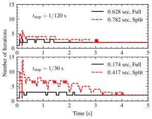
Figure 1: Statistics of the simulation performance for the IEEE 14-bus system using different integration step sizes.

Figure 1 compares the number of iterations and simulation time for the full and the split formulations in the IEEE 14-bus system. Two simulation step sizes are compared, namely, $1/120~{}\rm sec$ and $1/30~{}\rm sec$, where the former is widely used in commercial tools. It is expected that reducing the step size by a factor of four would result in four times the computational load in residual building and equation solving but partially compensated by the reduction in iteration number. Both the full and split formulations with different step sizes yield the same dynamic response trajectory and are thus omitted due to page limits.

The following characteristics are observed and analyzed:

1. The more efficient approach is full DAE formulation with a relatively large step size. Even with 15 more algebraic variables, the full DAE is considerably and consistently faster.

2. A small step size reduces the number of iterations due to the reduced gap between the split equations and the DAE. But it increases the computation time due to the step number increase.

3. The split DAE benefits less than the full formulation from a larger step size due to the increased difficulty in convergence.

III-A2 CURENT North America 944-bus model

This test system is a medium-size case with a large variety of generator, exciter, turbine governor, and power system stabilizer models. A total of 76 GENROU devices are in use. The applied disturbances are a bus-to-ground fault at $t=0.1~{}\rm sec$ and its clearance by a line trip at $t=0.2~{}\rm sec$.

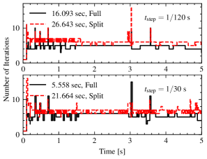
Figure 2: Simulation performance of the CURENT 944-bus system.

Figure 2 shows the computational performance for the CURENT system. Due to the model complexity such as limiters, the iteration counts do not exhibit decreasing trend for the five seconds simulated. It can be observed that the full DAE with a large step size is leading in performance. Also, the split DAE benefits even less from the step size reduction, merely reducing the time from $26.64~{}\rm sec$ to $21.66~{}\rm sec$ due to the increased number of iterations.

III-A3 Fictitious Polish 9241-bus system

This case is created from the 9241-bus system [5] by adding generators, exciters, and turbine governors with generic parameters to represent large systems. The full DAE of the system consists of 14,450 states and 61,833 algebraic variables, including those for 1,445 GENROU devices. The applied disturbance is a generator trip at Bus 190 at $t=0.1~{}\rm sec$.

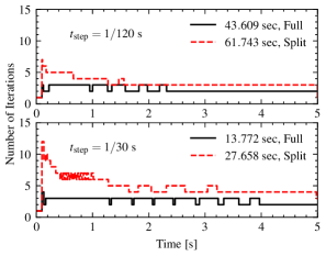
Figure 3: Simulation performance of the 9241-bus system.

The full and split formulations yield the same transient trajectories for the two step sizes. The computational performance follows the same observations as the previous two cases. Comparing all the three test cases, we observe and generalize the following:

1. The full DAE can consistently scale by roughly a factor of three, namely, increasing the step size from $1/120~{}\rm sec$ to $1/30~{}\rm sec$ reduces the run time by 3x. The factor of three is a result of roughly a quarter of the computational load that is offset by a slightly higher iteration count.

2. The split DAE is less deterministic in terms of computational scalability. The speed-up factor for a quadruple step size reduces the run time by approximately half at most, depending on the system dynamics.

III-B Renewable Generation Models

The full and split formulation of the renewable energy converter model (REGC_A) and its electric control model (REEC_A) are compared. For the REGC_A model, the low-voltage active power management output equations are split. For the REEC_A model, the voltage deviation equation, and the additional current injection equations are split. Note that all these equations are linear. Simulations are first performed using the IEEE 14-bus system, where 80% of the capacity on Bus 3 is replaced with two converters. A bus-to-ground fault is applied to Bus 6, followed by a line trip to clear the fault.

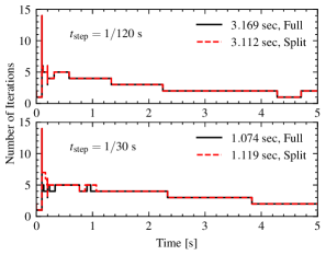
Figure 4: Simulation performance of the IEEE 14-bus system with renewables.

Figure 4 plots the simulation performance for the two formulations with different step sizes. In this case, the split formulation has much less impact compared with those for the GENROU model. Still, for $t=1/30~{}\rm sec$, multiple runs show that the split formulation is consistently slower by several percent. For $t=1/120~{}\rm s$, the two formulations are close in performance with no consistent winner.

The minor performance difference is due to the linearity of the equations that are split, as well as the relatively small size of the test system. Input changes to these equations result in linear corrections to the output, so that the gap between the split variables and the full DAE solution can remain small. Also, for $t=1/120~{}\rm sec$, given the same iteration count shown in Figure 4, the full DAE formulation with a larger DAE require more time to build, factorize, and solve.

Next, the performance of the full and the split formulations are compared using the 9241-bus system. A pair of renewable energy converters and electrical control models are attached to each bus with a synchronous generator to substitute for 10% of the active and reactive power outputs. The number of algebraic equations for the full DAE and the split DAE is 116,743 and 110,963, respectively. Both formulations have 28,900 differential states. A bus-to-ground fault is applied at Bus 4 at $t=0.1~{}\rm sec$ and cleared at $t=0.2~{}\rm sec$.

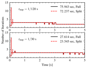
Figure 5: Simulation performance of the 9241-bus system with renewables.

Figure 5 shows the performance results. In this case, even for the step size of $1/30~{}\rm sec$, the convergence patterns are similar for both formulations. In other words, the split of the linear equations does not incur significant difficulty in convergence. Regardless of the step size, the full DAE formulation is consistently slower than the split formulation due to the larger size of the DAE.

IV Conclusions

This letter investigates the impact of the treatment of internal algebraic variables on transient simulation performance. The impacts are studied on synchronous generator models and renewable converter models in systems of various sizes. Our conclusions are:

1. The performance of the full and the split formulations depend on the equations being split and the size of the system.

2. For nonlinear algebraic equations like the flux linkage equations the synchronous generators, the more computationally efficient approach is to keep the variables in the DAE so that the iteration count can remain low when a large step size is applied.

3. Splitting linear equations, such as the ones in the converters, from the full DAE does not incur significant increases in the iteration count but can reduce the size of the Jacobian matrix, which is a significant factor for large systems.

References

- [1] Federico Milano “Power System Modelling and Scripting” In Power System Modelling and Scripting Berlin, Heidelberg: Springer, 2010
- [2] Peter W. Sauer, M. A. Pai and J. H. Chow “Power System Dynamics and Stability: With Synchrophasor Measurement and Power System Toolbox” Hoboken, NJ, USA: IEEE Press, Wiley, 2017
- [3] Hantao Cui, Fangxing Li and Kevin Tomsovic “Hybrid Symbolic-Numeric Framework for Power System Modeling and Analysis” In IEEE Transactions on Power Systems 36.2, 2021
- [4] Hantao Cui “ANDES - Python Software for Symbolic Power System Modeling and Numerical Analysis” URL: https://github.com/cuihantao/andes
- [5] Ray Daniel Zimmerman, Carlos Edmundo Murillo-Sánchez and Robert John Thomas “MATPOWER: Steady-State Operations, Planning, and Analysis Tools for Power Systems Research and Education” In IEEE Transactions on Power Systems 26.1, 2011, pp. 12–19