Degrees of Freedom and Information Criteria for
the Synthetic Control Method

Abstract

We provide an analytical characterization of the model flexibility of the synthetic control method (SCM) in the familiar form of degrees of freedom. We obtain estimable information criteria. These may be used to circumvent cross-validation when selecting either the weighting matrix in the SCM with covariates, or the tuning parameter in model averaging or penalized variants of SCM. We assess the impact of car license rationing in Tianjin and make a novel use of SCM; while a natural match is available, it and other donors are noisy, inviting the use of SCM to average over approximately matching donors. The very large number of candidate donors calls for model averaging or penalized variants of SCM and, with short pre-treatment series, model selection per information criteria outperforms that per cross-validation.

Keywords: Synthetic Controls, Model Selection, Information Criteria, Degrees of Freedom, Lagrange Multiplier Theory, Chinese Automotive Industry.

1 Introduction

The synthetic control method has become a standard regression tool in economics, political science, and a handful of other fields. See abadie2021using for a recent survey and pedagogical introduction. As such, methodological research has endeavored to append the synthetic control estimator with standard regression output. This includes confidence intervals, $p$-values, etc Abadie . (2010); Chernozhukov . (2018); Cattaneo . (2021).

Our primary contribution is to produce one such standard regression output statistic, the degrees of freedom. We find that the degrees of freedom, or effective number of estimated parameters, of the synthetic control method without covariates is one less than the expected number of donors having nonzero estimated coefficients. We obtain a more general result covering the case with covariates, where an interesting phase transition is uncovered.

Our motivation for producing this as of yet unavailable statistic is two-fold. First, the question “does the synthetic control method overfit?” is, as we argue below, nontrivial and important. The degrees of freedom offer a clear cut and intuitive answer to that question. We find that SCM does not overfit in most seminal applications we revisited. It does however overfit in “high-dimensional” applications such as the one we investigate in this paper.

Second, we produce information criteria for synthetic control methods. We find that, in applications with very many donors and short pre-treatment series, overfitting (through model selection flexibility) does arise and regularization is required. The short pre-treatment series make it such that cross-validation strategies perform poorly. An information criterion, which assesses the out-of-sample performance of the estimator evaluated on the entire pre-treatment data, is expected to do better. Equipped with closed form expressions for the degree of freedom that have sample analogs, we produce just such information criteria and indeed observe (in simulation and placebo cases) that they outperform cross-validation in terms of producing accurate counterfactual time series and treatment effect estimates.

Importantly, the produced information criteria can also be used to select the weighting matrix in the synthetic control problem with covariates, see problem formulation (3)-(5).

Degrees of freedom

Degrees of freedom expressions are inherently interesting for the synthetic control method. Indeed, consider two of the more striking –and attractive– features of the synthetic control method, typically at display in its standard output. We reproduce in Figure 1 the output of abadie2010synthetic as an example. First, the fitted regression coefficient estimates typically exhibit substantial sparsity; the synthetic control is a linear combination of a few donors, with many donors getting an estimated weight of zero. Second, the observed and fitted paths, before treatment, often suggest a high in-sample fit, as is the case in Figure 1.

These two features capture our motivation for inquiring into the degrees of freedom of the synthetic control method. The high degree of sparsity in the estimated regression coefficients suggests the possibility of extensive implicit model selection. Given that the series being fitted are often short, one may worry that this additional model flexibility brings about overfitting, and that this in fact what explains the surprising quality of the in-sample fit, hence casting doubt on the quality of the forecast and treatment effect estimates.

The question “does synthetic control overfit?” thus stands open. On the one hand, best subset selection with sample size and number of active independent variables typical of synthetic control applications would be expected to overfit (see Figure 2). On the other hand, placebo exercises in which one forecasts non-treated series and compares the forecasted to the realized series often suggest a reasonable quality of forecast (e.g., abadie2010synthetic). This motivates the development of an analytical measure of the model flexibility of the method, the most compelling of which is, in our opinion, its degrees of freedom.

Information criteria

The wide applicability of the synthetic control method has brought applied analysts to consider “high-dimensional” applications –i.e., with many donors– even though the training, or pre-treatement, period may be short. Such applications of course raise a priori concerns about overfitting, and these have brought about the development of penalized (abadie2021penalized) and model averaging (kellogg2020combining) methods, all of which require the specification of a tuning parameter. Typically, such tuning parameters are estimated by cross-validation, with different specific algorithms proposed by different authors, see Table 1.

CV method	Reference
Rolling window	kellogg2020combining
Pre-Intervention Holdout Validation on the Treated	abadie2015comparative, xu2017generalized,
	abadie2021penalized,
	ben2021augmented
Leave-one-out Validation on the Untreated	doudchenko2016balancing,
	abadie2021penalized

Table 1: Survey of cross-validation procedures suggested in the synthetic controls literature.

Cross-validation is also called upon in synthetic control applications to estimate the weighting matrix of the inner-problem in the synthetic control method with covariates. See (3)-(5) below for details about the construction of synthetic controls using covariates.

However, cross-validation is often ill-suited for model selection with the synthetic control method. Predominant cross-validation strategies for the synthetic control method are collected in Table 1. On the one hand, “pre-intervention holdout validation on the treated” is a data-splitting procedure; the estimator is trained on a first half of the pre-treatment data, and the second half is used as a test set. As such, we may expect it to be severely biased with short pre-treatment series; conceptually, the synthetic control method trained on, say, half of the pre-treatment data may behave very differently than that trained on the whole pre-treatment data. On the other hand, the “leave-one-out validation on the untreated” approach treats a donor as a placebo to-be-treated unit, and uses the post-treatment data as a test set. It ignores the true to-be-treated unit, and averages over the post-treatment forecast error of a selection of such placebo to-be-treated units. It relies on the assumption that, in the absence of a treatment effect, the conditional distribution of any donor –perhaps after some preselection– given the other donors is the same as that of the to-be-treated unit given the donors. Since we typically conceive of the to-be-treated unit as being in or near the convex hull formed by the active donors (abadie2021using), this comes as a rather unpalatable assumption.

As investigated in kellogg2020combining, the pre-intervention holdout approach may produce a misleading estimate of the prediction mean-squared error. kellogg2020combining instead propose to use rolling-window cross-validation which they find to perform best, at least for the MASC estimator (defined below). As detailed below, the procedure remains data hungry, and we are well motivated to consider out-of-sample error estimation methods that assess the performance of the synthetic control method trained on the entire pre-treatment data of the to-be-treated unit itself.

A classical alternative to cross-validation is to compare models using an information criterion (claeskens2008model). Information criteria append to the in-sample loss a penalty for model flexibility, thus allowing for the comparison of models of different flexibility while training them on the entire pre-treatment data.

The challenge in producing information criteria is to give a computable expression for a penalty term capturing model flexibility. As detailed in Section 3 below, this exercise is intimately tied to the estimation of degrees of freedom.

Impact of rationing on the demand for cars

The aforementioned methodological developments are of general interest but were, for the authors, motivated by the analysis of the market for new automobiles in China after the introduction of rationing. We investigate model specific changes in sales in Tianjin following the introduction of a lottery-auction hybrid for the distribution of car licenses. In order to build counterfactual –as if there had been no rationing– time series for each individual car model, the synthetic control method turns out to be a natural choice but falls prey to overfitting, and penalized synthetic controls (abadie2021penalized) and model-averaged synthetic controls (kellogg2020combining) are more reliable. However, cross-validation performs poorly for tuning parameter estimation and we are able to carry out a more robust analysis using our information criteria instead. We present model specific treatment effects of the policy, thus allowing for a detailed study of the market for new cars in Tianjin.

This is a novel, or at least uncommon, application of the synthetic control method. While a natural match is available –the same car model in an untreated city– it is very noisy. By instead averaging over many approximate matches, we can produce a synthetic control having a much smaller variance than the natural donor does, at a relatively small cost in bias.

Our methodological contributions can be succinctly summarized as follows. We produce information criteria for the synthetic control method. In the classical case of the synthetic control method with covariates, this allows for the selection of the weighting matrix. In the case of the penalized synthetic control method as well as that of the model averaged synthetic control method, this allows for the selection of the tuning parameter controlling model selection. Importantly, model selection based on the information criteria circumvents cross-validation, which we argue and demonstrate can be misleading in practice. We furthermore produce closed form degrees of freedom estimates for the synthetic control method, with or without covariates, as well as for its penalized and model averaged extensions. These may be reported, for instance, alongside output such as that in Figure 1.

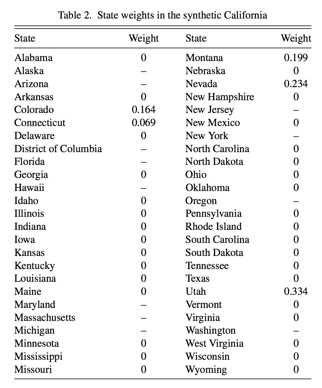
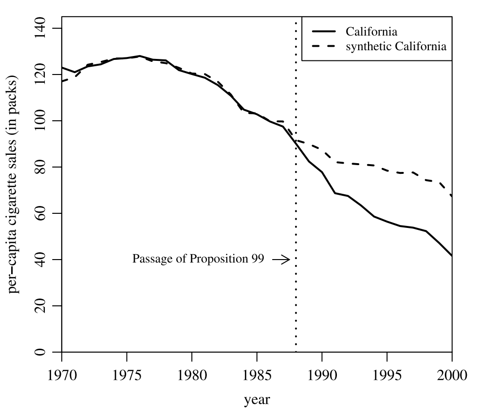
Figure 1: Synthetic control output of California Proposition 99 investigation.

The remainder of the article is divided as follows. Section 2 defines the synthetic control method and its penalized and model averaging extensions. Section 3 produces the information criteria and degrees of freedom estimates for the different methods. Section 4 uses some of the herein developed methodology to study the impact of license rationing on the sales of individual car models in Tianjin. Section 5 discusses and concludes.

2 The Synthetic Control Method

We are interested in the classical synthetic control method, and particularly interested in its penalized and model averaging extensions.

2.1 The Synthetic Control Method without Covariates

Given an observed series $\mathbf{Y}\in\mathbb{R}^{n}$ and $p$ observed series from “donors” collected as a matrix $\mathbf{X}\in\mathbb{R}^{n\times p}$, the vector of optimal donor weights $\hat{\beta}$ is the solution of the program

$$\min_{\beta}\left\|\mathbf{Y}-\mathbf{X}\beta\right\|_{2}$$ (1)

subject to

$$\mathbf{1}_{p}^{T}\beta=1,\ \beta\geq 0,$$ (2)

where the inequality applies pointwise to vectors.

The standard regression output of the synthetic control method contains a table of regression coefficient estimates, as well as a plot of the observed series before and after treatment, overlaid with the treated unit’s series fitted by synthetic control method before treatment, and forecasted after treatment. Because the forecasted series is a function of untreated units –called “donors”– estimated on pre-treatment data, it is interpreted as forecasting a non-treated counterfactual –a “synthetic control”– for the treated unit. The difference between the realized and forecasted series provides an estimate of the treatment effect.

2.2 The Synthetic Control Method with Covariates

In some cases, $n_{cov}$ “covariate” variables are believed to satisfy –at least approximately– the same linear relationship as the aforementioned series, and the coefficient $\beta$ is constrained to be a synthetic control solution for these covariates. Let the matrix $\mathbf{D}\in\mathbb{R}^{n_{\mathrm{cov}}\times p}$ and the vector $\mathbf{Z}\in\mathbb{R}^{n_{\mathrm{cov}}}$ collect the independent and dependent covariate variables, respectively. The optimal solution $\hat{\beta}$ is then obtained by solving the following two-level program,

$$\min_{V,\beta}\left\|\mathbf{Y}-\mathbf{X}\beta\right\|_{2}$$ (3)

subject to

$$\beta\in\arg\min_{\beta}\left\|\mathbf{Z}-\mathbf{D}\beta\right\|_{V}$$ (4)

$$\mathbf{1}_{p}^{T}\beta=1,\ \beta\geq 0,\ V\succeq 0\ \mathrm{and\ diagonal},$$ (5)

where $\left\|\mathbf{A}\right\|_{V}=\mathbf{A}^{T}V\mathbf{A}$ and $\left\|\mathbf{A}\right\|_{2}=\left\|\mathbf{A}\right\|_{I}$ for compatible matrices.

The diagonal matrix $V$ effectively weighs the “observations” of the inner regression problem, and as such some researchers may prefer to consider it as a hyperparameter, to fit using an out-of-sample criteria. Indeed, we may pick $V$ by cross-validation, solving at each iteration the problem (3)-(5) with $V$ fixed. This is a suggestion of abadie2015comparative.

2.3 The Penalized Synthetic Control Method

In settings where there are many donors relative to the number of pre-treatment time periods, one may be concerned about overfitting. Indeed, such a relatively large number of donors makes it more likely to find a linear combination of donors that closely matches the to-be-treated unit, even though they in fact have little predictive power. In particular, a collection of very “far away” donors may give a tight in-sample fit, even though we may have had an a priori belief that such “far away” donors are each poor individual matches and are expected as such to make for a poor synthetic control. We may therefore want to limit the choice of donors by relying on the conventional prior belief that donors more “similar” to the to-be-treated unit make for more reliable donors, in the specific sense that they offer a better out-of-sample forecast.

A natural way to implement such a prior belief for frequentist estimation is to add to the objective function a shrinkage term penalizing coefficients that puts more weight on a priori bad matches. This was suggested in abadie2010synthetic and implemented in abadie2021penalized. The estimator $\hat{\beta}_{\mathrm{pen}}$ is defined as the minimand of the penalized synthetic control objective

$$\min_{\beta}\left\|\mathbf{Y}-\mathbf{X}\beta\right\|_{2}^{2}+\lambda\sum_{i=1}^{p}\beta_{i}\left\|\mathbf{Y}-\mathbf{X}_{i}\right\|_{2}^{2}$$ (6)

subject to

$$\mathbf{1}^{T}\beta=1,\ \beta\geq 0,$$ (7)

where $\mathbf{X}_{j}$ is the $j^{\mathrm{th}}$ column of $\mathbf{X}$. Note that $\lambda$ must be selected by the user.

2.4 The Matching and Synthetic Control Estimator

An alternative to penalizing with matching distance is to instead implement model averaging with the matching estimator. kellogg2020combining argue that the model averaging approach outperforms the penalty approach in some typical applications. Model averaging likewise relies on estimation of out-of-sample fit in order to determine a tuning parameter.

The matching estimator $\hat{\beta}_{\mathrm{ma}}(m)$ solves the problem

$$\min_{\beta}\sum_{i=1}^{p}\beta_{i}\left\|\mathbf{Y}-\mathbf{X}_{i}\right\|_{2}$$

subject to

$$\mathbf{1}^{T}\beta=1,\ 0\leq\beta\leq 1/m,$$

This program is solved by setting $\beta_{i}=1/m$ for the $m$ donor units $i$ with smallest distance $\left\|\mathbf{Y}-\mathbf{X}_{i}\right\|_{2}$, and setting all other entries of $\beta$ to zero.

The matching and synthetic control estimator (MASC) is defined as

$$\hat{\beta}_{\mathrm{masc}}=\lambda\hat{\beta}_{\mathrm{ma}}(m)+(1-\lambda)\hat{\beta}_{\mathrm{sc}},$$ (8)

where $\lambda\in\left[0,1\right]$ is a tuning parameter, $\hat{\beta}^{\mathrm{sc}}$ is the synthetic control regression coefficient, and $\hat{\beta}^{\mathrm{ma}}(m)$ is the matching coefficient from the implementation with $m$ matches. A motivation for model averaging with matching is to tradeoff interpolation and extrapolation biases, see kellogg2020combining for a complete discussion.

Note that the synthetic control method with covariates could be penalized or used as the synthetic control estimate for the MASC estimator. Given theory for the synthetic control method with covariates, the theory for its penalized and model averaging extensions is immediate.

3 Information Criteria and Degrees of Freedom

Because the selection of the tuning parameter $\lambda$ in (6)-(7) and (8), or of the weighting matrix $V$ in (3)-(5), boils down to comparing models of different flexibility, we want to use a measure of out-of-sample performance as our criteria. One such natural notion is the error between the model’s fitted values and the target regression function, the conditional expectation. Specifically, we want to select a model, or tuning parameter, to minimize

$$\mathcal{R}:=E\left\|\hat{\mathbf{Y}}-E\left[\mathbf{Y}\left|\mathbf{X}\right.\right]\right\|_{2}^{2},$$ (9)

where $\hat{\mathbf{Y}}\in\mathbb{R}^{n}$ are the fitted values produced by the selected model. Since the goal is model selection, we will care about the risk only up to a constant. Note that

$$\mathcal{R}\propto E\left\|\mathbf{Y}-\hat{\mathbf{Y}}\right\|_{2}^{2}+2E\left\langle\hat{\mathbf{Y}},\varepsilon\right\rangle,$$ (10)

where $\varepsilon=\mathbf{Y}-E\left[\mathbf{Y}\left|\mathbf{X}\right.\right]$.

The cross-validation approach is understood to estimate

$$\mathcal{CV}:=E\left\|\mathbf{Y}_{\mathrm{new}}-\hat{\mathbf{Y}}_{\mathrm{new}}\right\|_{2}^{2},$$

where $\left(\mathbf{X}_{\mathrm{new}},\mathbf{Y}_{\mathrm{new}}\right)$ is an observation drawn from the same data generating process as, but not included in, the data set which the model forecasting $\mathbf{Y}_{\mathrm{new}}$ with $\hat{\mathbf{Y}}_{\mathrm{new}}$ was trained on. Observe that

$$\mathcal{R}\propto\mathcal{CV},$$

which is to say both the risk estimation approach and the cross-validation approach are maximizing out-of-sample fit according to the same population target, up to proportionality.

Our first contribution will be to produce an estimable expression for (10). To accomplish this, we rely on modern theory for degrees of freedom (meyer2000degrees, zou2007degrees) based on Stein’s lemma and the computation of divergences. Stein’s lemma requires the Gaussian assumption

$$\mathbf{Y}|\mathbf{X}\sim N\left(E\left[\mathbf{Y}|\mathbf{X}\right],\Sigma_{Y|X}\right).$$ (11)

This assumption is discussed in detail in Section 4, and extension to non-Gaussian distributions is discussed in Section 3.4.

Assuming (11) and almost differentiability (see Section A.4), Stein’s Lemma (stein1981estimation) states that

$$Cov\left(\left.Y_{i},\hat{Y}_{i}\right|\mathbf{X}\right)=\sigma_{i}^{2}E_{Y|X}\left[\frac{\partial\hat{Y}_{i}}{\partial Y_{i}}\right].$$ (12)

This is a simple yet powerful result. While the left-hand side of (12) is intractable, the right-hand may be computed in a straightforward fashion. Specifically, given adequate theory, the right-hand side may be estimated in closed form.

Under the Gaussian assumption (11), expression (10) is equivalently expressed as

$$\mathcal{R}\propto E\left\|\mathbf{Y}-\hat{\mathbf{Y}}\right\|_{2}^{2}+2E\left[\sum_{i=1}^{n}\sigma_{i}^{2}E_{Y|X}\left[\frac{\partial\hat{Y}_{i}}{\partial Y_{i}}\right]\right],$$ (13)

where $\sigma_{i}^{2}=V\left(\left.Y_{i}\right|\mathbf{X}\right)$.

Two observations are in order. First, remark that we never invoked independence nor homoskedasticity to produce expression (13). This is particularly convenient given the time series nature of data in some synthetic control applications.

Second, as we will argue in our application of interest, we will typically not believe that the paths of the donor series, $\mathbf{X}$, will differentially inform the variance of the to-be-treated unit at different periods. Specifically, we find it plausible that the homoskedasticity assumption

$$\sigma_{i}^{2}=\sigma^{2},\forall i,$$ (14)

for some $\sigma^{2}$, often holds at least approximately. The homoskedasticity assumption is further discussed in Section 3.4. Note that this assumption is also important for estimation given that the typically short pre-treatment series make difficult the estimation of heteroskedastic variances without engaging with rather cavalier assumptions.

Specifically, under homoskedasticity, expression (13) rewrites as

$$\mathcal{R}\propto IC:=E\left\|\mathbf{Y}-\hat{\mathbf{Y}}\right\|_{2}^{2}+2\sigma^{2}\mathrm{df}\left(\hat{\mathbf{Y}}\right),$$ (15)

where

$$\mathrm{df}\left(\hat{\mathbf{Y}}\right)=\frac{1}{\sigma^{2}}\sum_{i=1}^{n}Cov\left(\left.Y_{i},\hat{Y}_{i}\right|\mathbf{X}\right)=E\left[\mathrm{Tr}\left(E\left[\left.\nabla\hat{\mathbf{Y}}\right|\mathbf{X}\right]\right)\right].$$

Expression (15) is our main estimand of –proportional– risk. The key is to develop theory that produces computable estimates of the divergence $\nabla\hat{\mathbf{Y}}$. We do so in Section 3.1, and produce sample analogs of (15) in Section 3.3.

We remark that under homoskedasticity, the risk expression (15) relates in an immediate fashion to degrees of freedom as well as to more familiar expressions for information criteria, such as AIC, BIC or Mallow’s $C_{p}$.

Finally, remark that using Stein’s lemma and computable expressions for the divergence, we obtain an analytical and estimable expression for $\mathrm{df}\left(\hat{\mathbf{Y}}\right)$ in order to quantify analytically the model flexibility of the synthetic control method in typical applications. In Section 3.2, we carry out such an inquiry, and answer our motivating question “does the synthetic control method overfit?”.

The intellectual history of this approach can be summarized as follows. stein1981estimation proved (12) and used it to produce (15), now called Stein’s unbiased risk estimate (SURE). This implicitly defines a general formulation for degrees of freedom as part of the “penalty term” in SURE, when the latter is thought of as in information criteria. The literature attributes to efron2004estimation and hastie1990generalized the definition of degrees of freedom in terms of covariance between observed and fitted values, which matches that deduced from the “penalty term” of SURE, before applying Stein’s lemma. meyer2000degrees used Stein’s lemma to compute the degrees of freedom for shape restricted regression, setting the stage for other such applications, amongst which we find he degrees of freedom of the lasso, a result first given in zou2007degrees and generalized in tibshirani2012degrees. General results producing degrees of freedom estimates for classes of models are given in kato2009degrees and chen2020degrees.

3.1 Divergence Expressions for the Synthetic Control Method

Once a tractable analytic expression obtains for the divergence, the risk estimate and degrees of freedom obtain upon verifying regularity conditions. However, computing the divergence in specific cases can be non-trivial. Correspondingly, as tibshirani2015stein point out, a small industry of computing divergences has blossomed. In this section we provide the divergence for the methods presented in Section 2.

For each estimator and a corresponding solution coefficient $\hat{\beta}$, let $\mathcal{A}=\mathcal{A}\left(\mathbf{Y}\right)$ be the active support corresponding to the solution $\hat{\beta}$. For synthetic control problems with covariates, let $\mathcal{M}=\left\{i:d_{i}\hat{\beta}-z_{i}\neq 0\right\}$ designate the set of indices of nonzero residuals in the inner problem, and let $\mathcal{E}=\left\{i:v_{i}>0\right\}$ designate the set of indices of strictly positive diagonal weights.

Proposition 1 (Divergence of SCM with covariates).

Suppose the process generating the conditioned upon design matrices $\mathbf{X}$ and $\mathbf{D}$ is uniformly continuous with respect to Lebesgue measure. Then, the fitted values vector $\hat{\mathbf{Y}}$ of the synthetic control method has divergence

$$\frac{\partial\hat{\mathbf{Y}}}{\partial\mathbf{Y}}=\Pi_{\mathcal{A}}-\mathbf{X}_{\mathcal{A}}\mathbf{G}_{\mathcal{A}}^{-1}\mathbf{D}^{*T}\left(\mathbf{D}^{*}\mathbf{G}_{\mathcal{A}}^{-1}\mathbf{D}^{*T}\right)^{-1}\mathbf{D}^{*}\mathbf{G}_{\mathcal{A}}^{-1}\mathbf{X}_{\mathcal{A}}^{T},$$

where

$$\mathbf{D}^{*}=\begin{cases}\mathbf{1}_{|\mathcal{A}|},&\left|\mathcal{M}\cap\mathcal{E}\right|\geq\left|\mathcal{A}\right|-1\\ \mathbf{D}_{\mathcal{M}\cap\mathcal{E}},&\left|\mathcal{M}\cap\mathcal{E}\right|<\left|\mathcal{A}\right|-1\end{cases},$$

with $\Pi_{\mathcal{A}}=\mathbf{X}_{\mathcal{A}}\left(\mathbf{\mathbf{X}_{\mathcal{A}}}^{T}\mathbf{X}_{\mathcal{A}}\right)^{-1}\mathbf{X}_{\mathcal{A}}^{T}$ , and $\mathbf{G}_{\mathcal{A}}=\mathbf{X}_{\mathcal{A}}^{T}\mathbf{X}_{\mathcal{A}}$.

The case without covariates obtains as the special case with $\mathbf{D}^{*}=\mathbf{1}_{|\mathcal{A}|}$

$$\frac{\partial\hat{\mathbf{Y}}}{\partial\mathbf{Y}} =\Pi_{\mathcal{A}}-\frac{1}{\sum_{i,j}\mathbf{G}_{i,j}^{-1}(\mathcal{A})}\mathbf{b}_{\mathcal{A}}\mathbf{b}_{\mathcal{A}}^{T},$$

where $\mathbf{b}_{\mathcal{A}}=\mathbf{X}_{\mathcal{A}}\left(\mathbf{X}_{\mathcal{A}}^{T}\mathbf{X}_{\mathcal{A}}\right)^{-1}\mathbf{1}_{|\mathcal{A}|}$.

Proposition 2 (Divergence of penalized SCM).

Suppose the process generating the conditioned upon design matrices $\mathbf{X}$ and $\mathbf{D}$ is uniformly continuous with respect to Lebesgue measure. Then, the fitted values vector $\hat{\mathbf{Y}}$ of the penalized synthetic control method has divergence

$$\frac{\partial\hat{\mathbf{Y}}}{\partial\mathbf{Y}}=\Pi_{\mathcal{A}}-\lambda\pi_{\mathcal{A}}^{T}\left(\mathbf{1}_{p}\mathbf{Y}_{\mathcal{A}}^{T}-\mathbf{\mathbf{X}_{\mathcal{A}}}^{T}\right)-\pi_{\mathcal{A}}^{T}\mathcal{G}_{\mathcal{A}}\pi_{\mathcal{A}}$$

$$+\lambda\mathbf{X}_{\mathcal{A}}\mathbf{G}_{\mathcal{A}}^{-1}\mathcal{G}_{\mathcal{A}}\mathbf{G}_{\mathcal{A}}^{-1}\left(\mathbf{1}_{|\mathcal{A}|}\mathbf{Y}_{\mathcal{A}}^{T}-\mathbf{\mathbf{X}_{\mathcal{A}}}^{T}\right),$$

where $\mathbf{D}^{*}$, $\Pi_{\mathcal{A}}$ and $\mathbf{G}_{\mathcal{A}}$ are defined as in Proposition 1, $\pi_{\mathcal{A}}=\left(\mathbf{\mathbf{X}_{\mathcal{A}}}^{T}\mathbf{X}_{\mathcal{A}}\right)^{-1}\mathbf{X}_{\mathcal{A}}^{T}$, and $\mathcal{G}_{\mathcal{A}}=\mathbf{D}^{*T}\left(\mathbf{D}^{*}\mathbf{G}_{\mathcal{A}}^{-1}\mathbf{D}^{*T}\right)^{-1}\mathbf{D}^{*}$

In the case of the penalized synthetic control method without covariates, i.e., with $\mathbf{D}=\mathbf{1}_{|\mathcal{A}|}^{T}$, the expression for the divergence simplifies significantly, and may be given as

$$\frac{\partial\hat{\mathbf{Y}}}{\partial\mathbf{Y}}=\left(1+\lambda\right)\left(\Pi_{\mathcal{A}}-\frac{1}{\mathbf{1}_{|\mathcal{A}|}^{T}\mathbf{G}_{\mathcal{A}}^{-1}\mathbf{1}_{|\mathcal{A}|}}\mathbf{X}_{\mathcal{A}}\mathbf{G}_{\mathcal{A}}^{-1}\mathbf{1}_{|\mathcal{A}|}\mathbf{1}_{|\mathcal{A}|}^{T}\mathbf{G}_{\mathcal{A}}^{-1}\mathbf{X}_{\mathcal{A}}^{T}\right).$$

Proposition 3 (Divergence of the MASC estimator).

Suppose the process generating the conditioned upon design matrices $\mathbf{X}$ and $\mathbf{D}$ is uniformly continuous with respect to Lebesgue measure. Then, the fitted values vector $\hat{\mathbf{Y}}$ of the MASC estimator has divergence

$$\frac{\partial\hat{\mathbf{Y}}}{\partial\mathbf{Y}}=(1-\lambda)\frac{\partial\mathbf{X}\hat{\beta}_{\mathrm{sc}}}{\partial\mathbf{Y}},$$

where $\frac{\partial\mathbf{X}\hat{\beta}_{\mathrm{sc}}}{\partial\mathbf{Y}}$ is given in Proposition 1.

3.2 The Degrees of Freedom of the Synthetic Control Method

The divergence being the key ingredient of the computational formula for the degrees of freedom, we obtain as corollaries to the results of the previous subsection the degrees of freedom of the methods under study, sometimes in rather elegant closed form expressions.

Recall that our definition of degrees of freedom for a model and its fitted values $\hat{\mathbf{Y}}$ is

$$\mathrm{df}\left(\hat{\mathbf{Y}}\right)=\frac{1}{\sigma^{2}}\sum_{i=1}^{n}Cov\left(\left.Y_{i},\hat{Y}_{i}\right|\mathbf{X}\right),$$

assuming (14) holds. This is an attractive measurement of model flexibility. Indeed, define the noise perturbations $\varepsilon_{i}=Y_{i}-E\left[\left.Y\right|\mathbf{X}\right]$, $i=1,...,n$, then the definitional equivalence $Cov\left(\left.Y_{i},\hat{Y}_{i}\right|\mathbf{X}\right)=Cov\left(\left.\varepsilon_{i},\hat{Y}_{i}\right|\mathbf{X}\right)$ makes explicit that $\mathrm{df}\left(\hat{\mathbf{Y}}\right)$ is measuring how much the fitted values are adapting to noise. A familiar instance of degrees of freedom is the number of regression coefficients in ordinary least-squares (OLS). We indeed obtain that statistic back, as a special case of the more general definition. For instance, for OLS with nonsingular design matrix $\mathbf{X}\in\mathbb{R}^{n\times p}$, under assumptions (11) and (14), application of Stein’s lemma delivers the familiar expression

$$\mathrm{df}\left(\hat{\mathbf{Y}}_{\mathrm{ols}}\right)=E\left[\mathrm{Tr}\left(\mathbf{X}\left(\mathbf{X}^{T}\mathbf{X}\right)^{-1}\mathbf{X}^{T}\right)\right]=p,$$

where $\hat{\mathbf{Y}}_{\mathrm{ols}}=\mathbf{X}\left(\mathbf{X}^{T}\mathbf{X}\right)^{-1}\mathbf{X}^{T}\mathbf{Y}$.

We are therefore able to quantify the model flexibility, or “effective number of coefficients”, of the synthetic control method. Consider the case of the synthetic control method without covariates. Quite remarkably, we find that even though implicit –and sometimes extensive– model selection is carried out by the synthetic control method as it selects the active set –the donors with nonzero weight– the expected effective model flexibility remains that of a linear regression with sum-to-one constraint using only the selected donors. In other words, the implicit model selection is carried out at no additional cost in degrees of freedom.

Proposition 4.

Suppose $\mathbf{Y}$ follows the probability law stipulated in (11) and (14). Then, for any $\mathbf{X}$, the synthetic control fitted values $\mathbf{X}\hat{\beta}$ have degrees of freedom

$$df\left(\mathbf{X}\hat{\beta}\right)=E\left[\mathrm{rank}\left(\mathbf{X}_{\mathcal{A}}\right)\right]-1,$$

where $\mathcal{A}=\mathcal{A}\left(\mathbf{Y}\right)$ is the active support corresponding to solution $\hat{\beta}\left(\mathbf{Y}\right)$.

With continuous data, the result is even more directly interpretable and applicable, as it can be formulated directly in terms of the nonzero weight coefficients.

Corollary 1.

Suppose that, in addition to the conditions required in Proposition 4, the conditioned upon $\mathbf{X}$ was generated by a process that is uniformly continuous with respect to Lebesgue measure. Then, for any $\mathbf{X}$, the synthetic control fitted values $\mathbf{X}\hat{\beta}$ have degrees of freedom

$$df\left(\mathbf{X}\hat{\beta}\right)=E\left|\mathcal{A}\right|-1.$$

Figure 2 illustrates the theory on simulated data. We compare with the famous lasso result (zou2007degrees), which states that $df\left(\mathbf{X}\hat{\beta}_{\mathrm{Lasso}}\right)=E\left|\mathcal{A}_{\mathrm{Lasso}}\right|$, where $\mathcal{A}_{\mathrm{Lasso}}$ is the index set of the active independent variables in the lasso regression.

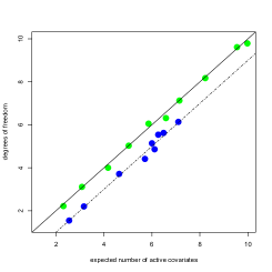
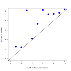
Figure 2: Degrees of freedom of the synthetic control method without covariates (blue) and of the lasso (green) on the left-hand side, and of the best subset selection regression on the right-hand side.

The right-hand side plot of Figure 2 illustrates the “real cost” of unrestricted model selection in terms of degrees of freedom and potential overfitting. The degrees of freedom of the best subset selection method, with respect to the size of the subset, are presented for comparison with their synthetic control analog. While a synthetic control fitted model has degrees of freedom one smaller than the expected number of covariates, we can see that the explicit model search introduces much more model flexibility.

Our main interest lies in model selection with penalized and model averaged methods, we are therefore interested in their degrees of freedom.

Proposition 5 (Degrees of Freedom of Penalized Synthetic Controls).

Suppose $\mathbf{Y}$ follows the probability law stipulated in (11) and (14). For a conditioned upon $\mathbf{X}\in\mathbb{R}^{n\times p}$ drawn from a process that is uniformly continuous with respect to Lebesgue measure and $\lambda\geq 0$, the penalized synthetic controls fit $\mathbf{X}\hat{\beta}_{\mathrm{pen}}$ has degrees of freedom

$$df\left(\mathbf{X}\hat{\beta}_{\mathrm{pen}}\right)=(1+\lambda)(E|\mathcal{A}|-1).$$

Proposition 6 (Degrees of Freedom of MASC).

Suppose $\mathbf{Y}$ follows the probability law stipulated in (11) and (14). For a conditioned upon $\mathbf{X}\in\mathbb{R}^{n\times p}$ drawn from a process that is uniformly continuous with respect to Lebesgue measure, the MASC synthetic controls fit $\mathbf{X}\hat{\beta}_{\mathrm{masc}}$ has degrees of freedom

$$df\left(\mathbf{X}\hat{\beta}_{\mathrm{masc}}\right)=(1-\lambda)\left(E\left|\mathcal{A}\right|-1\right).$$

The condition that $\mathbf{X}\in\mathbb{R}^{n\times p}$ be drawn from a continuous process may be dropped altogether and Propositions 6 and 7 obtain with $\left|\mathcal{A}\right|$ everywhere replaced by $\mathrm{rank}\left(\mathbf{X}_{\mathcal{A}}\right)$.

In the more general case of the synthetic control method with covariates, we likewise obtain a closed form formula for the degrees of freedom. Not so surprisingly, adding “a few” covariates further constraints the estimator, thus decreasing the degrees of freedom. Perhaps more surprisingly, with “sufficiently many” covariates, the same objective function value in the inner problem may be given by a manifold of different weighting matrices in turn producing different fitted weights, thus eliminating the reduction in degrees of freedom correction and producing a problem with as many degrees of freedom as the synthetic control method without covariates.

The general expression for the degrees of freedom of the synthetic control method is given in the following proposition. Recall that $\mathcal{M}=\left\{i:d_{i}\hat{\beta}-z_{i}\neq 0\right\}$ designates the set of indices of nonzero residuals in the inner problem, and $\mathcal{E}=\left\{i:v_{i}>0\right\}$ designates the set of indices of strictly positive diagonal weights.

Proposition 7.

Suppose $\mathbf{Y}$ follows the probability law stipulated in (11) and (14). Then, assuming the conditioned upon $\mathbf{X}$ and $\mathbf{D}$ were drawn from a process that is uniformly continuous with respect to Lebesgue measure, the synthetic control fitted values $\mathbf{X}\hat{\beta}$ have degrees of freedom

$$df\left(\mathbf{X}\hat{\beta}\right)=E\left[\widehat{df}\left(\mathbf{X}\hat{\beta}\right)\right],$$

and

$$\widehat{df}\left(\mathbf{X}\hat{\beta}\right)=\begin{cases}\mathrm{rank}\left(\mathbf{X}_{\mathcal{A}}\right)-1,&\left|\mathcal{M}\cap\mathcal{E}\right|\geq\left|\mathcal{A}\right|-1\\ \mathrm{rank}\left(\mathbf{X}_{\mathcal{A}}\right)-\left|\mathcal{E}\backslash\mathcal{M}\right|-1,&\left|\mathcal{M}\cap\mathcal{E}\right|<\left|\mathcal{A}\right|-1\end{cases},$$

where $\mathcal{A}=\mathcal{A}\left(\mathbf{Y}\right)$, $\mathcal{M}=\mathcal{M}\left(\mathbf{Y}\right)$ and $\mathcal{E}=\mathcal{E}\left(\mathbf{Y}\right)$ are active sets corresponding to a solution $\hat{\beta}\left(\mathbf{Y}\right)$, with probability one.

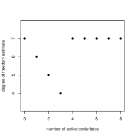
Figure 3: Illustration of the degrees of freedom of the synthetic control method with covariates. Suppose for expository purposes that, as we change the number of active covariates (nonzero coefficient, nonzero weight), the number of active donors (nonzero weight) remains constant. Then, we can clearly display the non-monotonicity of the degrees of freedom. Here we think of there being four active donors.

Typically, we find that $\left|\mathcal{E}\right|=p_{\mathrm{cov}}$. This is notable because the sample analog of the degrees of freedom formula is then made more computationally tractable.

Figure 4: Degrees of freedom of synthetic controls with covariates.

The variation of the degrees of freedom in Figure 4 is obtained by varying the number of covariates from 1 to 16. Again, the theory is nicely illustrated in simulations.

3.3 Information criteria for the synthetic control method

The information criteria estimate, the sample analog to (15), is

$$\widehat{IC}:=\left\|\mathbf{Y}-\hat{\mathbf{Y}}\right\|_{2}^{2}+2\hat{\sigma}^{2}\widehat{df}\left(\hat{\mathbf{Y}}\right).$$ (16)

All the degrees of freedom expressions $df\left(\hat{\mathbf{Y}}\right)$ derived in Section 3.2 are expectations of observed quantities, the latter are thus used as natural sample analogs $\widehat{df}\left(\hat{\mathbf{Y}}\right)$.

We estimate $\sigma^{2}$ as

$$\hat{\sigma}^{2}=\frac{1}{n}\sum_{i=1}^{n}\hat{\varepsilon}_{i}^{2},$$

where the residuals are from the unpenalized synthetic control method. This is the general approach suggested by friedman2001elements. Our experience from different simulation designs has been that, even though we obtain residuals from the unpenalized model, this approach tends to slightly overestimate the variance $\sigma^{2}$ and thus slightly overpenalize. As discussed in Section 4, because larger values of the tuning parameter effectively shrink the estimate towards the matching estimate and tend to produce an estimate that is more stable, we consider this “upward bias” as erring on the side of caution.

The estimated information criterion used to select the tuning parameter $\lambda$ when implementing the penalized synthetic control method is

$$\widehat{IC}_{\mathrm{pen}}(\lambda):=\left\|\mathbf{Y}-\hat{\mathbf{Y}}\right\|_{2}^{2}+2\hat{\sigma}^{2}\left(1+\lambda\right)\left(\left|\mathcal{A}\right|-1\right).$$

The estimated information criterion used to select the tuning parameter $\lambda$ when implementing the MASC estimator is

$$\widehat{IC}_{\mathrm{masc}}(\lambda):=\left\|\mathbf{Y}-\hat{\mathbf{Y}}\right\|_{2}^{2}+2\hat{\sigma}^{2}\left(1-\lambda\right)\left(\left|\mathcal{A}\right|-1\right).$$

Remark that $\lambda$ affects $\widehat{IC}_{\mathrm{pen}}(\lambda)$ and $\widehat{IC}_{\mathrm{masc}}(\lambda)$ both directly and through $\left|\mathcal{A}\right|$.

3.4 Discussion of assumptions

The homoskedasticity assumption (14) may appear limiting to some users and this concern warrants discussion.

First, the independence and homoskedasticity assumption may be relaxed, but at the cost of additional assumptions. Specifically, liu1994siegel gives a multivariate generalization of Stein’s Lemma according to which the information criteria becomes

$$E\left\|\mathbf{Y}-\hat{\mathbf{Y}}\right\|_{2}^{2}+2E\left[\mathrm{Tr}\left(\Sigma_{Y|X}E\left[\left.\nabla\hat{\mathbf{Y}}\right|\mathbf{X}\right]\right)\right].$$

The form is more general, but brings about the challenge of estimating $\Sigma_{Y|X}$. It may be estimated in different ways. If one is willing to make the necessary stationarity and specification assumptions, one may for instance fit an ARMA model on the residuals and use the implied covariance matrix as an estimate. If one wants to allow misspecification but is willing to further rely on the Gaussianity assumption, then one may compute the conditional covariance in terms of the unconditional covariances as $\Sigma_{Y}-\Sigma_{YX}\Sigma_{X}^{-1}\Sigma_{XY}$, where $X$ only contains the selected donors and stationarity assumptions must still be made.

Second, we can see from the simulations in Section 4.2 that while the simulated data displays heteroskedasticity –commensurate to that of the observed data, with respect to which we largely reject a White test for homoskedasticity– the estimate of degrees of freedom is remarkably robust.

The Gaussianity assumption (11) may likewise appear limiting in practice. While developing an estimator under Gaussian assumptions is by no means exceptional, it remains important to ask if such an assumption can be relaxed, and if we are robust to its misspecification.

First, the Gaussianity assumption may be relaxed, or rather exchanged for another distributional assumption. Indeed, chetverikov2021cross extend formula (12) to non-Gaussian distributions, under the condition that random variables distributed according to said distributions obtain as a smooth transformation of Gaussian random variables. See their Lemma 9.4. A general expression then obtains for the degrees of freedom under a smoothness assumption on the transformation, see their Assumption 3 and Lemma 8.3. This is to say, the available theory does not allow us to do away with any distributional assumption, but nevertheless accommodates a large family of distributional assumptions rather than just the Gaussian one.

Second, we can see from the simulations in Section 4.2 that while the semi-synthetic data is decidedly not Gaussian, our estimate of the degrees of freedom, and thus of out-of-sample performance, is remarkably robust.

4 Forecasting Counterfactual Car Sales under Rationing in Tianjin

In Tianjin, on December 16, 2013, the municipal government introduced a hybrid half-lottery and half-auction system for the procurement of drivers’ licenses which heavily rationed the number of licenses emitted. This was done in order to limit pollution from car emissions, which had become a public health hazard.

Because the auction allowed wealthier individuals a better chance of obtaining a license, the rationing induced a change in the population of car buyers, and therefore a change in the demand for different models (li2018better).

This change in demand may be non trivial. While daljord2021black document the change in the population of car buyers in Beijing when there is a lottery without auction and the licenses are transacted on a black market alone, they do not study the impact of rationing on the demand for specific models. However, manufacturers and policymakers ought to be interested in the impact of such a policy on the sales of car models of different prices and fuel consumption.

Specifically, we are interested in establishing model specific counterfactual demand, and thus the impact on sales, of many individual car models.

The strategy is to use the city of Shijiazhuang to build counterfactuals. Shijiazhuang is comparable to Tianjin in that, for instance, it is geographically close and has a population on the same order of magnitude (15 vs 11 millions). Crucially, Shijiazhuang did not have rationing and we observe sales data for that city.

We highlight two features of the empirical analysis. The first feature is that we use the synthetic control method not because we are missing a good match, but to combine many good albeit noisy matches so to attenuate variance while minimizing cost in bias. Bias and variance are traded off according to the tuning parameter of the penalized or model averaged synthetic control.

The second feature is that we consider the simulation and data analysis in conjunction, and simulate from a data generating process meant to emulate that of the observed data. We do this for two reasons. First, the simulation should be thought of as part of the application; to best carry model selection (i.e., picking the tuning parameter), we must first elect a model selection method, and since we do not have enough observations to compare empirically model selection methods on observed data (a very data hungry procedure), we resort to simulated data. Second, we are interested in the simulation for its own sake; in order to properly assess how practical the theory is, we want to carry out robustness checks on simulated yet realistic data.

4.1 Empirical Approach

An apparently natural approach would be to use matching with a single match. Indeed, all models investigated are sold in both Shijiazhuang and Tianjin, and thus the Shijiazhuang sales for, say, a Toyota Tercel, make a natural counterfactual for the Toyota Tercel sales in Tianjin, post rationing. However, the relatively small number of sales for any given model makes the time series relatively noisy and methodology tackling this issue ought to be considered and compared.

On the one hand, filtering is a natural way to tackle the issue of noisy donors data. Specifically, we want to average over similar time series and thus reduce noise at little cost in bias. Intuitively, the underlying demand patterns for analogous models from different brands such as, say, a Toyota Tercel and a Honda Civic, may be very similar, thus allowing for variance reduction at little cost in bias when averaging over both series to build a counterfactual series for the Tercel. The synthetic control method is specifically aimed at building a control unit by averaging over multiple possible controls. We thus consider it as a natural alternative to matching.

Note that this is, to the best of our knowledge, a novel use of the synthetic control method. The SCM is typically used when an obvious match cannot be found; here, a natural match can be found, but it is noisy and we prefer to combine with slightly imperfect matches in order to attenuate the noise.

On the other hand, regularization is a natural way to tackle the issue of a noisy to-be-treated, or outcome variable, particularly when there are many independent variables. This suggests the use of a regularized alternative to synthetic controls, such as the MASC estimator (kellogg2020combining) or penalized synthetic controls (abadie2021penalized). Of course the probability simplex constraint, as well as the covariates if any are used, act as a form of regularization. We find that the additional regularization induced by the above two methods is beneficial in our application.

4.2 Simulation

We consider three complementary simulation designs. First, we generate series using a block bootstrap approach. While this does not allow us to compute and compare with an analytical expression for –or an arbitrarily accurate estimate of– true risk, it allows us to assess, albeit in a blunt manner, the extent of overfitting under minimal assumptions. Second, we consider a Gaussian factor model. In that design, the Gaussian assumption underlying the theory applies, and we can furthermore compute the true risk for comparison. Finally, we keep with the factor model but sample the outcome unit’s residuals from their empirical distribution, thus assessing the robustness of the theory and the relative performance of different model selection methods in a more realistic design in which we can still compute the true risk.

An ad hoc but model-free and transparent simulation approach is to bootstrap the multivariate time series. We sample with replacement from the pre-treatment data a new data set of full length using the stationary bootstrap of politis1994stationary. Because for any thus bootstrapped data set the placebo post treatment period may be composed of the same observation as the training, pre-treatment period, this approach will not perfectly mimic the out-of-sample performance of a given estimator; in fact, it is expected to underestimate the out-of-sample error due to overfitting. Nevertheless, under stationarity, the procedure will naturally preserve properties of the distribution of the data and may display some, though not the full extent, of the overfitting behavior of more flexible models.

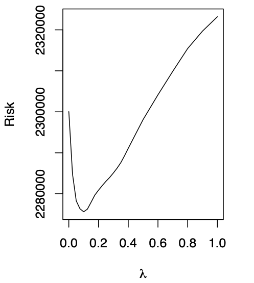
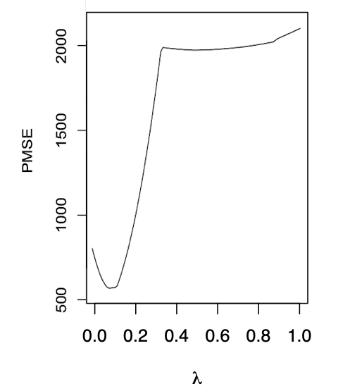
Figure 5: Empirical evidence of overfitting. Proportional risk where the averaged over draws of the block bootstrap (LHS), and 12 month average squared forecast error of the zero treatment effect Shijiazhuang after treatment time in Tianjin (RHS).

On the left-hand side of Figure 5, we see that the estimate of the proportional risk (13), averaged over bootstrap samples, displays excess model flexibility for small values of the tuning parameter $\lambda$. Exploratory data analysis offers an additional comparison; on the right-hand side of Figure 5, we plot the 12 month average squared error forecast in Shijiazhuang, where the true treatment effect is known to be zero. We again see evidence of overfitting. The out-of-sample performance improves as we first increase the tuning parameter $\lambda$ away from zero. Since the treatment effect, as illustrated in Figure 9, is often very sensitive to the value of the tuning parameter at small values, this simulation evidence suggests the importance of using a penalized or model averaging method.

While our interest is in the quality of fit of the synthetic control method, we use and estimate a more involved but more flexible model to simulate from. Motivated by the theoretical insight of abadie2010synthetic and by the successful implementation on Current Population Survey (ferman2019synthetic), we fit a factor model.

Specifically, the model for our second simulation design is

$$Y_{t}=\delta_{t}+\psi_{t}^{T}L_{1}+U_{1t},\ t=1,...,T,$$ (17)

$$X_{it}=\delta_{t}+\psi_{t}^{T}L_{i}+U_{it},\ i=2,...,p,\ t=1,...,T,$$ (18)

where $U_{it}$ follows an Gaussian ARMA($p,q$) for each $i$, and $\psi_{t}\sim N(0,I)$, and is independent across $i$.

Exploratory data analysis as well as the bootstrap exercise display overfitting, as illustrated in Figure 5. We thus require a data generating process that captures this feature of the data, especially since our simulation exercise pertains particularly to tuning parameter selection for penalized synthetic controls. While one could fit (17) and (18) jointly and estimate $L_{1}$, $L_{2}$,…,$L_{p}$ at once, such a factor structure would not capture the –perhaps approximately– sparse representation of the best linear predictor. Instead, we consider the best linear predictor

$$E^{*}\left[Y|X\right]=X\omega^{*}$$

and model the to-be-treated unit’s factor loadings as

$$L_{1}=L_{-1}\omega^{*},$$

where $L_{-1}=(L_{2},L_{3},...,L_{p})$.

We argue that this is a natural modeling assumption. abadie2010synthetic suggest as a theoretical framework a factor model with perfect fit on the outcome values and covariates. We consider the assumption of exact fit on the conditional mean to be a weaker requirement. Likewise, kellogg2020combining note that such linearity of the factor loadings is in fact necessary for there to be no interpolation bias. This assumption is also important for modeling the overfitting. Since the vector of nonnegative weights $w$ is constrained to sum to one, overfitting does not arise just from there being many donors, but from there being many models to select from and amongst which some do not carry enough signal for accurate forecasting. As a plug-in for $\omega^{*}$, we use $\hat{\omega}$ from the unpenalized synthetic control fit.

The key of the simulation exercise is to be able to compare with the ground truth, specifically to be able to compute the conditional expectation $E\left[\mathbf{Y}\left|\mathbf{X}\right.\right]$. Indeed, we consider the Gaussian factor model with

$$E\left[\psi_{t}\right]=0,\ E\left[\psi_{t}\psi_{t}^{T}\right]=I,\ E\left[\mathbf{U}_{t}\mathbf{U}_{t}^{T}\right]=\Sigma,$$

where $\Sigma$ is assumed to be diagonal. Specifically, we assume that

$$\left(\begin{array}[]{c}Y_{t}\\ \mathbf{X}_{t}\end{array}\right)\sim N\left(\delta_{t}\mathbf{1}_{p},\mathbf{L}\mathbf{L}^{T}+\Sigma\right),$$

where $\mathbf{X}_{t}=\left(X_{2t},...,X_{pt}\right)^{T}$and $\mathbf{L}=\left(L_{1},...,L_{p}\right)^{T}\in\mathbb{R}^{p\times r}$, whence conditional expectations $E\left[\left.Y_{t}\right|\mathbf{X}_{t}\right]$ obtain in closed form for all $t$, and the true proportional risk may be computed easily.

For the third simulation design, we draw the innovations $U_{it}$ from a non-Gaussian distribution in order to assess robustness to failure of distributional assumptions. Note that the conditional expectation nevertheless obtains in closed form. See Appendix C for details.

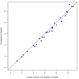
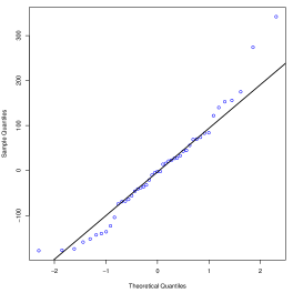
Figure 6: Study of Robustness. Estimated degrees of freedom versus true degrees of freedom for Gaussian factor model (top left), Estimated degrees of freedom versus true degrees of freedom for Gaussian factor model with empirical residuals (top right), histogram of empirical residuals (bottom left), quantile-quantile plot of empirical residuals (bottom right).

In Figure 6 we study the robustness of our estimate of degrees of freedom, and hence of the risk, to the ubiquitous failure of the the Gaussian assumption. We see in the histogram (bottom-left panel) and quantile-quantile plot (bottom-right panel) that the fitted residuals are decidedly not Gaussian, but the quantile-quantile plot nevertheless suggests a moderate enough departure from Gaussianity that our estimate of degrees of freedom may still be accurate enough to be useful. This is validated by the top right panel of Figure 6, which shows that the estimated degrees of freedom still line up well with the truth, in expectation. Remarkably, from inspecting the plot, the estimate does not seem to do any worse on average than in the case where the errors are Gaussian and the theory applies (top-left panel).

Note that we mimic the heteroskedasticity observed in the true data generating process. The robustness to distributional assumptions discussion above therefore applies to heteroskedaticity as well.

While the simulation exercise is intrinsically motivated by the need to assess the robustness of SURE to distributional assumptions, it is likewise motivated by the need to select a model selection method for the application whose data generating process the simulation emulates.

To that end, Figure 7 displays typical output from this simulation. We see in the top-left panel that the simulation design produces a U-shape for the true proportional risk which is similar to those observed in the bootstrap exercise and data exploratory exercise, displayed in Figure 5 for comparison.

Figure 7: Risk and risk estimates evaluated on a realization of simulated data. The top-left panel presents the risk. The top-right panel presents the SURE estimate of (proportional) risk. The bottom-left panel presents the estimate of risk according to ”pre-intervention holdout” cross-validation. The bottom-right panel presents the estimate of risk according to ”leave-one-out” cross-validation.

The information criteria based on Stein’s unbiased risk estimate (SURE) captures this true pattern, and selects approximately the same model. Horizontal and vertical cross-validations display substantially different patterns, and do not select the oracle model, i.e., that selected according to the population risk.

	Gaussian				Empirical				block bootstrap
	MSE$(\hat{\tau}_{1})$	MSE$(\hat{\tau}_{12})$	MSE$(\hat{\lambda})$	MSE$(\widehat{\mathrm{\mathcal{R}}})$	MSE$(\hat{\tau}_{1})$	MSE$(\hat{\tau}_{12})$	MSE$(\hat{\lambda})$	MSE$(\widehat{\mathrm{\mathcal{R}}})$	MSE$(\hat{\tau}_{1})$	MSE$(\hat{\tau}_{12})$
Risk	6.78	6.55	0	0	1.17	1.75	0	0	*	*
SURE*	6.88	6.75	0.007	1.7	1.15	1.30	0.02	4.3	*	*
SURE	6.96	6.79	0.009	16.3	1.15	1.32	0.04	17.4	3.10	6.22
CV-horizontal	7.14	6.99	0.02	18.1	3.89	3.79	0.15	20.4	4.50	9.21
CV-vertical	7.29	6.81	0.03	18.9	1.35	1.31	0.03	20.1	3.59	8.06
Rolling window	7.31	6.85	0.04	19.8	3.32	3.92	0.19	19.0	3.43	7.92

Table 2: Accuracy of treatment effect estimates from different model selection procedures. For SURE* and SURE, $MSE(\widehat{\mathrm{\mathcal{R}}})$ gives the mean-squared error of the estimated proportional risk (10) divided by $n$; for the horizontal, vertical, and rolling window cross-validation, $MSE(\widehat{\mathrm{\mathcal{R}}})$ gives the mean-squared error of the estimated mean-squared error of the one-step forecast of the conditional expectation, so to make entries of the column comparable. $MSE(\hat{\lambda})$ gives the mean-squared error of $\hat{\lambda}$ with respect to $\lambda^{*}$, the minimizer of the true risk. SURE* employs the information criteria with the true variance $\sigma$.

In Table 2, we consider different methods under the three aforementioned simulation designs. The information criteria performs almost uniformly better, and in the case of short lag forecast, it selects models that tend to do better at estimating the treatment effect, as quantified by the mean-squared error.

From the simulation exercise we conclude that the information criterion is more reliable for studying the data at hand. We thus elect the information criteria approach as our model selection method for analyzing the data.

4.3 Data Analysis

Having chosen the information criteria approach (16) as our model selection method, we may now carry out the regression exercise.

We first investigate in detail the impact of rationing for a single, popular model, the Toyota Corolla. This procedure can be automated and allows for the joint analysis of a selection of models, which we carry out subsequently.

In preprocessing, we pass the data through an MA(3) filter. The start date of the time series is January 2012, and the end data is December 2014.

Analysis for a single model

We analyze in isolation the impact of rationing on the demand for the Toyota Corolla. At a high level, the core task is to build a counterfactual; the time series of demand for the Corolla had there not been rationing.

As intuited and anticipated above, pure matching approaches deliver a poor counterfactual for the to-be-treated unit. Whether we match the Corolla in Tianjin to the Corolla in Shijiazhuang, or to the nearest model in Tianjin according to the penalty term, so in the $\ell_{2}$ sense, we get an unconvincing fit even as assessed by the plot of the time series. See Figure 8.

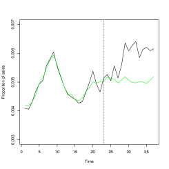
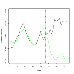
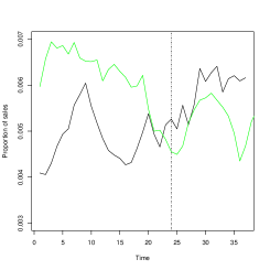
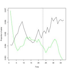
Figure 8: Observed and fitted time series. Synthetic control without penalty term (top-left), penalized synthetic controls with penalty term and tuning parameter estimated by SURE (top-right), matching by model (bottom-left), matching by distance (bottom-right). Note that the tuning parameter as estimated by cross-validation is zero, i.e. $\lambda_{\mathrm{cv}}^{*}=0$, and therefore its output is that of the top-left plot.

This motivates the use a of synthetic control, a match that is averaged over multiple donors, and is thus expected to have lower variance. Concerns of model flexibility –there are 175 donors after eliminating models that were either introduced after the beginning of our time series or discarded before the end– and noisy to-be-treated series motivate the use of penalized synthetic controls (abadie2021penalized). As is generally the case, two general approaches avail to estimate the tuning parameter of the penalty term: the cross-validation approach and the information criteria approach.

Our data set is too limited to assess in a data-driven way which method best estimates out-of-sample mean-squared error; such “cross-validation of cross-validation methods” are generally and obviously very data hungry procedures. Hence, in order to select the appropriate method of estimation of out-of-sample error, we mimicked as best as we could the data generating process of the application. In simulation exercise of Section 4.2, we found that the information criteria approach provided a more accurate estimate or prediction error and, crucially, produced a model that better predicted treatment effects, especially at short horizons.

It may be that certain time invariant variables improve the fit when used as covariates. Two natural covariates are the stock price of the model’s brand and the average –over time– of its outcome data. We consider the penalized synthetic control model with these two covariates, and select both $\lambda$ and $V$ according to our information criteria. The selected model put full weight on the covariate constructed as an average of outcome data, and had worse information criterion than the model without covariates. We therefore opt for proceeding without covariates.

We assess the plausibility of the homoskedasticity invoked in (15) in the manner of the White test (white1980heteroskedasticity, breusch1979simple). The $R^{2}$ of the regression of the squared residuals of the synthetic control regression with tuning parameter $\hat{\lambda}_{IC}$ on a time index and its square, as well as the donor series and their square, is $0.57$, with a $p$-value $0.02$. This suggests a moderate amount of heteroskedasticity and, in light of our simulation study, leaves us sufficiently confident that the theory will remain by and large reliable.

Remark that the choice of model selection method is consequential. As is well exemplified in the case of the Corolla, two different regression model selection methods can select substantially different models, leading to different treatment effect estimates. As is immediate from Figure 9, the estimate of prediction mean-squared error is monotone in $\lambda$ according to cross-validation, detecting none of the expected overfitting. The plot of the estimated risk versus $\lambda$, according to the information criteria estimate, however presents the U-shape typical of overfitting scenarios; penalization for smaller values of $\lambda$ reduces overfitting and decreases the prediction error, but for too large values of $\lambda$ the regression underfits and the prediction error increases.

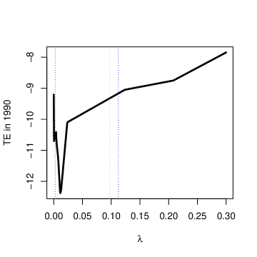
Figure 13: The treatment effect of the penalized estimator as a function of the tuning parameter $\lambda$ for the California Proposition 99 data. Vertical lines correspond to SURE with $\lambda=0.0025$ (green dash line), cross-validation on untreated produces $\lambda=0$, cross-validation with pre-intervention holdout validation on treated gives $\lambda=0.0975$ (gray dash line), cross-validation with rolling window gives $\lambda=0.1125$ (blue dash line). There are no covariates.

The implied difference on the treatment effect estimate is economically important. While the estimate calibrated by cross-validation predicts an increase in relative demand of 16% for the Corolla, the information criteria based estimate predicts an increase of 63%. Consider this in light of the right-hand side panel of Figure 9. There is a large change in the estimated treatment effect from a marginal increase in the tuning parameter $\lambda$ away from zero. This behavior has been, in our experience, recurrent over different models and in the different data sets we have investigated (e.g., California Proposition 99 data, Figure 13). Now note that the treatment effect estimate corresponding to the nonzero $\lambda_{\mathrm{IC}}^{*}$ is much more stable with respect to perturbations of the tuning parameter. As such, it makes us more confident in the reliability of the reported estimate, especially since standard linear model theory suggests that a modicum of penalization is beneficial in general (rao1995linear).

This difference in output from different model selection methodologies ought to be qualified. The conceptual motivation for penalizing is that we are confident, or have an a priori belief, that “nearby” donors are “better” donors; indeed, that is the motivation for matching in the first place. A more heavily penalized synthetic control estimate is less prone to use “far away” donors whose fluctuations may coincidentally cancel and produce a good in-sample fit without capturing signal. For instance, the linear combination of a luxury minivan, say the Buick GL8, and an ultra economical hatchback, say the Zotye Z100, may give a better in-sample fit for the corolla than does the linear combination of the Tercel and Corolla itself but, especially since there are many more donors than training periods, we would suspect that this is an instance of overfitting via model selection.

A larger tuning parameter forces the estimator towards the matching estimator, and away from perhaps coincidental linear combinations of donors producing a tighter in-sample fit. In a way that echoes model selection interpretation with the lasso –which forces the estimated regression function towards zero or another value considered a priori plausible– the more penalized estimate is more “conservative” in a desirable sense.

To what extent are we relying more on “far away” donors when we do not penalize? The penalty term $\sum_{i=1}^{p}\hat{\beta}_{i}\left\|\mathbf{Y}-\mathbf{X}_{i}\right\|_{2}^{2}$, where $\hat{\beta}_{i}$ is a function of $\lambda$, evaluates at 0.0001 for $\lambda_{\mathrm{cv}}^{*}=0$, which in this case is zero, and at 0.001 for $\lambda_{\mathrm{IC}}^{*}=0.3$. So, in the $\ell_{2}$ sense, the relevant donors are “on average” about three times farther from the donor unit in the unpenalized synthetic control estimate.

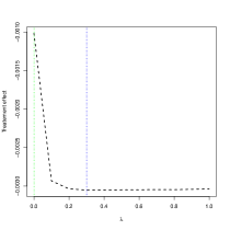
Figure 9: Estimate of out-of-sample mean squared error by cross-validation (left), information criteria (middle), and the one-year treatment effect estimate versus $\lambda$ (right) with vertical lines indicating $\lambda_{\mathrm{cv}}^{*}$ (green) and $\lambda_{\mathrm{IC}}^{*}$ (blue).

We thus find that, for the Corolla, proportional sales increased substantially due to the introduction of rationing, and the concentration of richer buyers. This is quite interesting. The Corolla is a mid range car –44th percentile for price, from low to high, of all observed models– and it was not ex ante obvious to us that it could be an common choice for auction or lottery winner. We do not attempt to differentiate between the two types of winners and leave this for further research, note however that such a question may be tackled using the optimal transport reduced form methodology developed in daljord2021black.

Figure 10: Histogram of treatment effects.

The analogous analysis for the Corolla using the MASC estimator is carried out in the Appendix, where we find comparable estimates of treatment effect.

Joint analysis for multiple models

We wish to investigate the heterogeneity in the treatment effect across different models. Did luxury cars indeed fare well under the new quota? What about low-end cars? To accommodate such considerations, we consider simultaneously the treatment effect estimates of multiple care models.

Figure 11: Heterogeneous treatment effects.

We consider the 26 models that sold more than 10,000 units over the period covered by the data and carry out the synthetic control regression for all models so to produce model specific counterfactual and treatment effect paths.

We carry out the White test for homoskedasticity, as described in the previous subsection, for each model. Out of the 26 models, 14 fail to reject the null of homoskedasticity with probability of type 1 error 0.05, and 21 fail to reject with probability of type 1 error 0.01. We cannot discard the presence of heteroskedasticity but, in light of the simulation evidence, it appears to be modest enough for our theory to be pertinent.

With all individual treatment effects in hand, we can produce their histogram and assess visually the distribution of treatment effects. The bulk of the distribution centers at a small positive increase in relative sales, with a longer, thinner left tail of large decreases in relative sails.

Of course this does not indicate which cars are being sold in greater or lesser proportions. In particular, we wonder if more expensive cars tend to be relatively more popular, once the population of car buyers is now in part composed of presumably wealthier auction winners. The immediate way to visualize this, which is accessible to us given the individual treatment effects, is to plot the treatment effect against path for each car. Figure 11 presents such a graphic. We see that all levels are decreasing, which was expected because of the massive reduction in total license emitted. However, we see a very minor reduction –in fact, it is a proportional increase– in sales of the high end Audi A6. Conversely, the Ford Focus, a low end car, sees one of the largest decreases in sales. Since the auction induced a greater concentration of wealthy buyers, this was expected. As described in detail above, the sales for the mid range Toyota Corolla are surprisingly robust to the reduction in the number of licenses and the resulting change in the composition of buyers. Meanwhile, two other mid range vehicles, the Volkswagen Bora and Jetta, fare much worse and see drops in sales comparable to that of the Focus.

Figure 12: Treatment effect versus price, given in proportional sales. The dashed line gives the OLS fit.

Figure 12 nevertheless confirms the expected pattern, overall. More expensive cars tend to see a smaller decrease in sales. The cars with the most extreme reduction in relative demand tend to be the cheapest.

5 Conclusion

When used in high-dimensional settings, regression methods are often appended with a penalty term to avoid overfitting, with the lasso being a popular example. The synthetic control method, a near cousin of the lasso, is no exception, and penalized and model averaging extensions have been developed to deal with high-dimensional settings. Such extensions require model selection, either according to cross-validation or to an information criteria. While information criteria are commonplace for the lasso, and the default in some packages, such methodology was missing for the synthetic control method. We have developed novel theory and methodology in order to carry out model selection according to an information criterion, and have argued that it is more reliable than cross-validation in our application of interest, and in what we find to be typical synthetic control applications.

The herein developed theory delivered degrees of freedom estimates for the synthetic control method. These in turn produced reassuring theoretical guarantees that the good in-sample fit of the method in early, seminal applications (e.g., abadie2003economic, abadie2010synthetic, abadie2015comparative) was due to the information content and not the flexibility of the synthetic control model.

In analyzing Chinese car sales data, we found that the synthetic control method could be profitably used for filtering when good matches are available but noisy. In our application, this called for the use of the model averaging or penalized variants of SCM in order to avoid overfitting, and of an information criteria to select the correct tuning parameter. Thus equipped, we were able to produce model specific treatment effect paths for a selection of cars.

Appendix A Lemmas and Proofs of Main Results

The argument is broken down into four sections. In Section A.1, we give a closed form expression for the divergence of the unpenalized and penalized least squares problem with linear equality constraint. In Section A.2, we show that for a given selection of active sets of nonzero donor weights, covariate residuals, and weighting matrix diagonal entries, synthetic control problems may be expressed as a least squares problem with equality constraints. Section A.3 shows that the conditions on the active sets with respect to which the problem is broken down into cases in Section A.2 are locally stable, implying that a linearly constrained least squares representation holds with probability one. Section A.4 combines the results of Sections A.1, A.2 and A.3 to prove the main result.

A.1 Divergence Expressions of Least Squares Problem with Linear Equality Constraints

The divergence obtains by differentiating a tractable expression for the fitted values. Our proof strategy will be to reformulate all instances as a problem of least-squares minimization subject to linear equality constraints. This is convenient because the divergence for such a problem obtains from elementary manipulations.

Proposition 8.

Let $\hat{\beta}$ be the solution of the unpenalized linearly constrained least-squares problem

$$\min_{\beta}\frac{1}{2}\left\|\mathbf{Y}-\mathbf{X}\beta\right\|_{2}^{2}$$ (19)

subject to

$$\mathbf{D}\beta=\mathbf{Z},\ \ \beta\geq 0,$$ (20)

where $\mathbf{X}\in\mathbb{R}^{n\times p}$ and $\mathbf{D}\in\mathbb{R}^{h\times p}$, $h\leq p$, both have full column rank. Then the divergence of $\mathbf{X}\hat{\beta}$ has closed form solution

$$\frac{\partial\mathbf{X}\hat{\beta}}{\partial\mathbf{Y}}=\mathbf{X}\left(\mathbf{X}^{T}\mathbf{X}\right)^{-1}\mathbf{X}^{T}-\mathbf{X}\left(\mathbf{X}^{T}\mathbf{X}\right)^{-1}\mathbf{D}^{T}\left(\mathbf{D}\left(\mathbf{X}^{T}\mathbf{X}\right)^{-1}\mathbf{D}^{T}\right)^{-1}\mathbf{D}\left(\mathbf{X}^{T}\mathbf{X}\right)^{-1}\mathbf{X}^{T},\$$

and its trace is

$$\mathrm{Tr}\left(\nabla\mathbf{X}\hat{\beta}\right)=\mathrm{rank}\left(\mathbf{X}\right)-h.$$

Proof.

The closed form expression for primal and dual solution pair obtains by direct calculation on the Lagrangian and an explicit expression is given in Section 16.2 of boyd2018introduction. The system can be solved for the primal solution $\hat{\beta}$ alone by inverting the Schur complement of the Gram matrix using the Woodbury identity, whence

$$\hat{\beta}=\left(\mathbf{X}^{T}\mathbf{X}\right)^{-1}\mathbf{X}^{T}\mathbf{Y}-\left(\mathbf{X}^{T}\mathbf{X}\right)^{-1}\mathbf{D}^{T}\left(\mathbf{D}\left(\mathbf{X}^{T}\mathbf{X}\right)^{-1}\mathbf{D}^{T}\right)^{-1}\mathbf{D}\left(\mathbf{X}^{T}\mathbf{X}\right)^{-1}\mathbf{X}^{T}\mathbf{Y}$$

$$+\left(\mathbf{X}^{T}\mathbf{X}\right)^{-1}\mathbf{D}^{T}\left(\mathbf{D}\left(\mathbf{X}^{T}\mathbf{X}\right)^{-1}\mathbf{D}^{T}\right)^{-1}\mathbf{Z}.$$

Therefore,

$$\mathrm{Tr}\left(\frac{\partial\mathbf{X}\hat{\beta}}{\partial\mathbf{Y}}\right) =\mathrm{Tr}\left(\mathbf{X}\left(\mathbf{X}^{T}\mathbf{X}\right)^{-1}\mathbf{X}^{T}-\mathbf{X}\left(\mathbf{X}^{T}\mathbf{X}\right)^{-1}\mathbf{D}^{T}\left(\mathbf{D}\left(\mathbf{X}^{T}\mathbf{X}\right)^{-1}\mathbf{D}^{T}\right)^{-1}\mathbf{D}\left(\mathbf{X}^{T}\mathbf{X}\right)^{-1}\mathbf{X}^{T}\right)$$

$$=\mathrm{rank}\left(\mathbf{X}\right)-\mathrm{Tr}\left(\mathbf{X}\left(\mathbf{X}^{T}\mathbf{X}\right)^{-1}\mathbf{D}^{T}\left(\mathbf{D}\left(\mathbf{X}^{T}\mathbf{X}\right)^{-1}\mathbf{D}^{T}\right)^{-1}\mathbf{D}\left(\mathbf{X}^{T}\mathbf{X}\right)^{-1}\mathbf{X}^{T}\right)$$

$$=\mathrm{rank}\left(\mathbf{X}\right)-\mathrm{Tr}\left(\mathbf{D}\left(\mathbf{X}^{T}\mathbf{X}\right)^{-1}\mathbf{X}^{T}\mathbf{X}\left(\mathbf{X}^{T}\mathbf{X}\right)^{-1}\mathbf{D}^{T}\left(\mathbf{D}\left(\mathbf{X}^{T}\mathbf{X}\right)^{-1}\mathbf{D}^{T}\right)^{-1}\right)$$

$$=\mathrm{rank}\left(\mathbf{X}\right)-\mathrm{Tr}\left(I_{h}\right).$$

 

Proposition 9.

Let $\hat{\beta}$ be the solution of the penalized linearly constrained least-squares problem

$$\min_{\beta}\frac{1}{2}\left\|\mathbf{Y}-\mathbf{X}\beta\right\|_{2}^{2}+\frac{1}{2}\lambda\sum_{i=1}^{p}\beta_{i}\left\|\mathbf{Y}-\mathbf{X}_{i}\right\|_{2}^{2}$$ (21)

subject to

$$\mathbf{D}\beta=\mathbf{Z},\ \ \beta\geq 0,$$ (22)

where $\mathbf{X}_{j}$ is the $j$-th column of $\mathbf{X}$. The divergence of $\mathbf{X}\hat{\beta}_{\text{psc}}$ has the closed-form expression

$$\nabla\mathbf{X}\hat{\beta}_{\text{psc}}= \mathbf{X}(\mathbf{X}^{T}\mathbf{X})^{-1}\mathbf{X}^{T}-\mathbf{X}(\mathbf{X}^{T}\mathbf{X})^{-1}\mathbf{D}^{T}\Bigg{(}\mathbf{D}(\mathbf{X}^{T}\mathbf{X})^{-1}\mathbf{D}^{T}\Bigg{)}^{-1}\mathbf{D}(\mathbf{X}^{T}\mathbf{X})^{-1}\mathbf{X}^{T}$$

$$-\lambda\mathbf{X}(\mathbf{X}^{T}\mathbf{X})^{-1}(\mathbf{1}_{p}\mathbf{Y}^{T}-\mathbf{X}^{T})+\lambda\mathbf{X}(\mathbf{X}^{T}\mathbf{X})^{-1}\mathbf{D}^{T}\Bigg{(}\mathbf{D}(\mathbf{X}^{T}\mathbf{X})^{-1}\mathbf{D}^{T}\Bigg{)}^{-1}\mathbf{D}(\mathbf{X}^{T}\mathbf{X})^{-1}\left(\mathbf{1}_{p}\mathbf{Y}^{T}-\mathbf{X}^{T}\right).$$

Proof.

The problem (21)-(22) has the Lagrangian function

$$\mathcal{L}=\frac{1}{2}\|\mathbf{Y}-\mathbf{X}\beta\|_{2}^{2}+\frac{1}{2}\lambda\sum\limits_{i=1}^{p}\beta_{i}\|\mathbf{Y}-\mathbf{X}_{i}\|_{2}^{2}+\xi^{T}(\mathbf{D}\beta-\mathbf{Z})$$

and KKT conditions

$$\cfrac{\partial\mathcal{L}}{\partial\beta}=-\mathbf{X}^{T}(\mathbf{Y}-\mathbf{X}\beta)+\frac{1}{2}\lambda\mathcal{Q}+\mathbf{D}^{T}\xi=\mathbf{0},\ \text{where}\ \mathcal{Q}=\left(\begin{matrix}\|\mathbf{Y}-\mathbf{X}_{1}\|_{2}^{2}\\ \vdots\\ \|\mathbf{Y}-\mathbf{X}_{p}\|_{2}^{2}\end{matrix}\right).$$

The optimality conditions can be rewritten in the matrix form

$$\left(\begin{matrix}\mathbf{X}^{T}\mathbf{X}&\mathbf{D}^{T}\\ \mathbf{D}&\mathbf{0}\end{matrix}\right)\left(\begin{matrix}\hat{\beta}\\ \hat{\xi}\end{matrix}\right)=\left(\begin{matrix}\mathbf{X}^{T}\mathbf{Y}-\frac{1}{2}\lambda\mathcal{Q}\\ \mathbf{Z}\end{matrix}\right).$$

Using the same approach as in unpenalized problem, we obtain the closed-form expression

$$\hat{\beta}= (\mathbf{X}^{T}\mathbf{X})^{-1}\mathbf{X}^{T}\mathbf{Y}-(\mathbf{X}^{T}\mathbf{X})^{-1}\mathbf{D}^{T}\Bigg{(}\mathbf{D}(\mathbf{X}^{T}\mathbf{X})^{-1}\mathbf{D}^{T}\Bigg{)}^{-1}\mathbf{D}(\mathbf{X}^{T}\mathbf{X})^{-1}\mathbf{X}^{T}\mathbf{Y}$$

$$+(\mathbf{X}^{T}\mathbf{X})^{-1}\mathbf{D}^{T}\Bigg{(}\mathbf{D}(\mathbf{X}^{T}\mathbf{X})^{-1}\mathbf{D}^{T}\Bigg{)}^{-1}\mathbf{Z}-\frac{1}{2}\lambda(\mathbf{X}^{T}\mathbf{X})^{-1}\mathcal{Q}$$

$$+\frac{1}{2}\lambda(\mathbf{X}^{T}\mathbf{X})^{-1}\mathbf{D}^{T}\Bigg{(}\mathbf{D}(\mathbf{X}^{T}\mathbf{X})^{-1}\mathbf{D}^{T}\Bigg{)}^{-1}\mathbf{D}(\mathbf{X}^{T}\mathbf{X})^{-1}\mathcal{Q}.$$

Note that $\cfrac{\partial\mathcal{Q}}{\partial\mathbf{Y}}=2\mathbf{1}_{p}\mathbf{Y}^{T}-2\mathbf{X}^{T}$. The closed form expression for the divergence of the penalized synthetic control problem obtains as

$$\cfrac{\partial\mathbf{X}\hat{\beta}}{\partial\mathbf{Y}}= \mathbf{X}(\mathbf{X}^{T}\mathbf{X})^{-1}\mathbf{X}^{T}-\mathbf{X}(\mathbf{X}^{T}\mathbf{X})^{-1}\mathbf{D}^{T}\Bigg{(}\mathbf{D}(\mathbf{X}^{T}\mathbf{X})^{-1}\mathbf{D}^{T}\Bigg{)}^{-1}\mathbf{D}(\mathbf{X}^{T}\mathbf{X})^{-1}\mathbf{X}^{T}$$

$$-\lambda\mathbf{X}(\mathbf{X}^{T}\mathbf{X})^{-1}(\mathbf{1}_{p}\mathbf{Y}^{T}-\mathbf{X}^{T})+\lambda\mathbf{X}(\mathbf{X}^{T}\mathbf{X})^{-1}\mathbf{D}^{T}\Bigg{(}\mathbf{D}(\mathbf{X}^{T}\mathbf{X})^{-1}\mathbf{D}^{T}\Bigg{)}^{-1}\mathbf{D}(\mathbf{X}^{T}\mathbf{X})^{-1}\left(\mathbf{1}_{p}\mathbf{Y}^{T}-\mathbf{X}^{T}\right).$$

 

The case without covariates produces a simpler expression for the divergence. Let $\mathbf{D}=\mathbf{1}_{p}^{T}$, we can have a more concise expression:

$$\cfrac{\partial\mathbf{X}\hat{\beta}}{\partial\mathbf{Y}}= \mathbf{X}(\mathbf{X}^{T}\mathbf{X})^{-1}\mathbf{X}^{T}-\mathbf{X}(\mathbf{X}^{T}\mathbf{X})^{-1}\mathbf{1}_{p}\Bigg{(}\mathbf{1}_{p}^{T}(\mathbf{X}^{T}\mathbf{X})^{-1}\mathbf{1}_{p}\Bigg{)}^{-1}\mathbf{1}_{p}^{T}(\mathbf{X}^{T}\mathbf{X})^{-1}\mathbf{X}^{T}$$

$$-\lambda\mathbf{X}(\mathbf{X}^{T}\mathbf{X})^{-1}\mathbf{1}_{p}\mathbf{Y}^{T}+\lambda\mathbf{X}(\mathbf{X}^{T}\mathbf{X})^{-1}\mathbf{1}_{p}\Bigg{(}\mathbf{1}_{p}^{T}(\mathbf{X}^{T}\mathbf{X})^{-1}\mathbf{1}_{p}\Bigg{)}^{-1}\mathbf{1}_{p}^{T}(\mathbf{X}^{T}\mathbf{X})^{-1}\mathbf{1}_{p}\mathbf{Y}^{T}$$

$$+\lambda\mathbf{X}(\mathbf{X}^{T}\mathbf{X})^{-1}\mathbf{X}^{T}-\lambda\mathbf{X}(\mathbf{X}^{T}\mathbf{X})^{-1}\mathbf{1}_{p}\Bigg{(}\mathbf{1}_{p}^{T}(\mathbf{X}^{T}\mathbf{X})^{-1}\mathbf{1}_{p}\Bigg{)}^{-1}\mathbf{1}_{p}^{T}(\mathbf{X}^{T}\mathbf{X})^{-1}\mathbf{X}^{T}$$

$$= (1+\lambda)\left[\mathbf{X}(\mathbf{X}^{T}\mathbf{X})^{-1}\mathbf{X}^{T}-\cfrac{1}{\mathbf{1}_{p}^{T}(\mathbf{X}^{T}\mathbf{X})^{-1}\mathbf{1}_{p}}\mathbf{X}(\mathbf{X}^{T}\mathbf{X})^{-1}\mathbf{1}_{p}\mathbf{1}_{p}^{T}(\mathbf{X}^{T}\mathbf{X})^{-1}\mathbf{X}^{T}\right].$$

A.2 Reformulation of Synthetic Control Method with Covariates

The nonlinear programming problem for the synthetic control method with covariates (3)-(5) is a bilevel programming problem. The lower-level problem, or inner problem, is a convex minimization problem, and the bilevel problem can therefore be recast as a single level problem in which the lower-level problem is replaced with its Karush Kuhn Tucker (KKT) conditions, as these precisely characterize the set of solutions of the inner problem, see dutta2006bilevel.

Let $\mathbf{V}=\mathrm{diag}(v)=\mathrm{diag}\left(v_{1},...,v_{n_{\mathrm{cov}}}\right)$, $d_{i}$ be the $i^{\mathrm{th}}$ row of $\mathbf{D}$, $z_{i}$ be the $i^{\mathrm{th}}$ entry of $\mathbf{Z}$, and reformulate (3)-(5) as

$$\min_{\beta,\lambda,\mu,v}\frac{1}{2}\left\|\mathbf{Y}-\mathbf{X}\beta\right\|_{2}^{2}$$

subject to

$$\mathbf{D}^{T}\mathbf{V}\left(\mathbf{D}\beta-\mathbf{Z}\right)+\lambda\mathbf{1}_{p}+\mu=\mathbf{0}_{p}$$

$$\beta\geq 0,\mu\geq 0,\mu\circ\beta=0$$

$$\mathbf{1}_{p}^{T}\beta=1,v\geq 0,$$

where $a\circ b=(a_{i}b_{i})_{i=1}^{p}$ stands for entry-wise multiplication, $\lambda$ is the Lagrangian multiplier for sum-to-one constraint, $\mu$ is the Lagrangian multiplier for the non-negative constraint.

By Lemmas 2, 3 and 4, $\mathcal{A}=\left\{i:\hat{\beta}_{i}>0\right\}$ is locally stable, and thus fixed with probability one in a neighborhood of the $\mathbf{Y}$. We abuse notation and let $d_{i}=d_{\mathcal{A},i}$ stand for the rows of $\mathbf{D}_{\mathcal{A}}$, as will be clear from context.

The corresponding Lagrangian is

$$\mathcal{L}\left(\beta_{\mathcal{A}},v,\lambda\right) =\frac{1}{2}\left\|\mathbf{Y}-\mathbf{X}_{\mathcal{A}}\beta_{\mathcal{A}}\right\|_{2}^{2}+\xi^{T}\left(\mathbf{D}_{\mathcal{A}}^{T}\mathbf{V}\left(\mathbf{D}_{\mathcal{A}}\beta_{\mathcal{A}}-\mathbf{Z}\right)+\lambda\mathbf{1}_{|\mathcal{A}|}\right)$$

$$+\lambda^{\prime}\left(\mathbf{1}_{|\mathcal{A}|}^{T}\beta_{\mathcal{A}}-1\right)+\delta^{T}v,$$

where $\xi\in\mathbb{R}^{|\mathcal{A}|}$, $\delta\geq\mathbf{0}_{n_{\mathrm{cov}}}$, and $\lambda^{\prime}\in\mathbb{R}$, and the KKT conditions are

$$\frac{\partial\mathcal{L}}{\partial\beta_{\mathcal{A}}} =-\mathbf{X}_{\mathcal{A}}^{T}\left(\mathbf{Y}-\mathbf{X}_{\mathcal{A}}\hat{\beta}_{\mathcal{A}}\right)+\sum\limits_{i=1}^{n_{\mathrm{cov}}}\left(\xi^{T}v_{i}d_{i}^{T}\right)d_{i}^{T}+\lambda^{\prime}\mathbf{1}_{|\mathcal{A}|}=\mathbf{0}_{|\mathcal{A}|},$$

$$\frac{\partial\mathcal{L}}{\partial v_{i}} =\left(d_{i}\beta_{\mathcal{A}}-z_{i}\right)d_{i}\xi+\delta_{i}=0,\ \ \text{for}\ i=1,...,n_{\text{cov}},$$

$$\frac{\partial\mathcal{L}}{\partial\lambda} =\mathbf{1}_{|\mathcal{A}|}^{T}\xi=0,$$

$$\frac{\partial\mathcal{L}}{\partial\lambda^{\prime}} =\mathbf{1}_{|\mathcal{A}|}^{T}\beta_{\mathcal{A}}-1=0.$$

Let $\mathcal{M}=\left\{i:d_{i}\hat{\beta}-z_{i}\neq 0\right\}$ designate the set of indices of nonzero residuals in the inner problem. Let $\mathcal{E}=\left\{i:v_{i}>0\right\}$ designate the set of indices of strictly positive diagonal weights.

The argument for deriving the reformulation is divided into cases. Proposition 10 covers the case in which $\left|\mathcal{A}\right|-1\leq\left|\mathcal{E}\cap\mathcal{M}\right|$, and the complement is divided into two cases, $|\mathcal{E}\cap\mathcal{M}|<|\mathcal{A}|-1\leq|\mathcal{E}|$, which is covered by Proposition 11, and $|\mathcal{E}\cap\mathcal{M}|\leq|\mathcal{E}|<|\mathcal{A}|-1$, which is covered by Proposition 12.

Proposition 10.

Suppose $\left|\mathcal{A}\right|-1\leq\left|\mathcal{E}\cap\mathcal{M}\right|$ and that the conditioned upon covariates $\mathbf{D}$ are drawn from a process that is uniformly continuous with respect to Lebesgue measure. Then problem (3)-(5) is equivalent to

$$\min_{\beta_{\mathcal{A}}}\frac{1}{2}\left\|\mathbf{Y}-\mathbf{X}_{\mathcal{A}}\beta_{\mathcal{A}}\right\|_{2}^{2}$$

subject to

$$\mathbf{1}_{|\mathcal{A}|}^{T}\beta_{\mathcal{A}}=1,$$

where $\mathcal{A}$ corresponds to a solution of problem (3)-(5).

Proof.

For $i\in\mathcal{E}$, complementary slackness requires that $\delta_{i}=0$, and

$$\left(d_{i}\hat{\beta}_{\mathcal{A}}-z_{i}\right)d_{i}\hat{\xi}=0\ \mathrm{for\ all}\ i\in\mathcal{E}\cap\mathcal{M},$$

where $d_{i}\beta_{\mathcal{A}}-z_{i}\in\mathbb{R}\backslash\{0\}$. With probability one, $\mathrm{rank}\left((\mathbf{D}_{\mathcal{E}\cap\mathcal{M},\mathcal{A}}^{T},\mathbf{1}_{|\mathcal{A}|})^{T}\right)=\min\{|\mathcal{E}\cap\mathcal{M}|,|\mathcal{A}|\}+1\geq\min\{|\mathcal{A}|-1,|\mathcal{A}|\}+1\geq|\mathcal{A}|$, implying that $\hat{\xi}=\mathbf{0}_{|\mathcal{A}|}$.

Therefore the KKT conditions $\frac{\partial\mathcal{L}}{\partial v_{i}}=0$ are vacuous, and the solution is defined by the system of conditions

$$\frac{\partial\mathcal{L}}{\partial\beta_{\mathcal{A}}} =-\mathbf{X}_{\mathcal{A}}^{T}\left(\mathbf{Y}-\mathbf{X}_{\mathcal{A}}\hat{\beta}_{\mathcal{A}}\right)+\lambda^{\prime}\mathbf{1}_{|\mathcal{A}|}=\mathbf{0}_{|\mathcal{A}|},$$

$$\frac{\partial\mathcal{L}}{\partial\lambda} =\mathbf{1}_{|\mathcal{A}|}^{T}\xi=0,\ \ \frac{\partial\mathcal{L}}{\partial\lambda^{\prime}}=\mathbf{1}_{|\mathcal{A}|}^{T}\beta_{\mathcal{A}}-1=0.$$

These correspond to the optimization program with Lagrangian

$$\mathcal{L}\left(\beta_{\mathcal{A}},\lambda\right)=\frac{1}{2}\left\|\mathbf{Y}-\mathbf{X}_{\mathcal{A}}\beta_{\mathcal{A}}\right\|_{2}^{2}+\lambda^{\prime}\left(\mathbf{1}_{|\mathcal{A}|}^{T}\beta_{\mathcal{A}}-1\right)$$

and constrained form

$$\min_{\beta_{\mathcal{A}}}\frac{1}{2}\left\|\mathbf{Y}-\mathbf{X}_{\mathcal{A}}\beta_{\mathcal{A}}\right\|_{2}^{2}$$

subject to

$$\mathbf{1}_{|\mathcal{A}|}^{T}\beta_{\mathcal{A}}=1,\ \beta_{\mathcal{A}}\geq 0.$$

 

Now we cover the intermediate case in which $\left|\mathcal{E}\cap\mathcal{M}\right|<\left|\mathcal{A}\right|-1<\left|\mathcal{E}\right|$.

Proposition 11.

Suppose $\left|\mathcal{E}\cap\mathcal{M}\right|<\left|\mathcal{A}\right|-1\leq\left|\mathcal{E}\right|$ and that the conditioned upon covariates $\mathbf{D}$ are drawn from a process that is uniformly continuous with respect to Lebesgue measure. Then problem (3)-(5) is equivalent to

$$\min\frac{1}{2}\left\|\mathbf{Y}-\mathbf{X}_{\mathcal{A}}\beta_{\mathcal{A}}\right\|_{2}^{2}$$

subject to

$$\mathbf{Z}_{\mathcal{E}\backslash\mathcal{M}}-\mathbf{D}_{\mathcal{E\backslash\mathcal{M}},\mathcal{A}}\beta_{\mathcal{A}}=0$$

$$\mathbf{1}_{|\mathcal{A}|}^{T}\beta_{\mathcal{A}}=1,$$

where the sets $\mathcal{A}$, $\mathcal{E}$, $\mathcal{M}$ correspond to a solution of problem (3)-(5).

Proof.

The lower-level programming problem is

$$\min_{\beta_{\mathcal{A}}}\frac{1}{2}\left\|\mathbf{Z}_{\mathcal{E}}-\mathbf{D}_{\mathcal{E},\mathcal{A}}\beta_{\mathcal{A}}\right\|_{\mathbf{V}_{\mathcal{E}}}$$

subject to

$$\mathbf{Z}_{\mathcal{E}\backslash\mathcal{M}}-\mathbf{D}_{\mathcal{E\backslash\mathcal{M}},\mathcal{A}}\beta_{\mathcal{A}}=\mathbf{0}_{\left|\mathcal{E\backslash\mathcal{M}}\right|}$$

$$\mathbf{1}_{|\mathcal{A}|}^{T}\beta_{\mathcal{A}}=1.$$

It has Lagrangian

$$\mathcal{L}_{\mathrm{lower}}=\frac{1}{2}\left\|\mathbf{Z}_{\mathcal{E}}-\mathbf{D}_{\mathcal{E},\mathcal{A}}\beta_{\mathcal{A}}\right\|_{\mathbf{V}_{\mathcal{E}}}+\varphi^{T}\left(\mathbf{Z}_{\mathcal{E}\backslash\mathcal{M}}-\mathbf{D}_{\mathcal{E\backslash\mathcal{M}},\mathcal{A}}\beta_{\mathcal{A}}\right)+\lambda\left(\mathbf{1}_{|\mathcal{A}|}^{T}\beta_{\mathcal{A}}-1\right),$$

and KKT conditions

$$\frac{\partial\mathcal{L}_{\mathrm{lower}}}{\partial\beta_{\mathcal{A}}} =\mathbf{D}_{\mathcal{E},\mathcal{A}}^{T}\mathbf{V}_{\mathcal{E}}\left(\mathbf{Z}_{\mathcal{E}}-\mathbf{D}_{\mathcal{E},\mathcal{A}}\beta_{\mathcal{A}}\right)+\lambda\mathbf{1}_{\left|\mathcal{A}\right|}+\mathbf{D}_{\mathcal{E\backslash M},\mathcal{A}}^{T}\varphi=0$$

$$\frac{\partial\mathcal{L}_{\mathrm{lower}}}{\partial\mu} =\mathbf{Z}_{\mathcal{E}\backslash\mathcal{M}}-\mathbf{D}_{\mathcal{E\backslash\mathcal{M}},\mathcal{A}}\beta_{\mathcal{A}}=\mathbf{0}_{\left|\mathcal{E\backslash\mathcal{M}}\right|}$$

$$\frac{\partial\mathcal{L}_{\mathrm{lower}}}{\partial\lambda} =\mathbf{1}_{|\mathcal{A}|}^{T}\beta_{\mathcal{A}}-1=0$$

The Lagrangian for the upper level problem is therefore

$$\mathcal{L} =\frac{1}{2}\left\|\mathbf{Y}-\mathbf{X}_{\mathcal{A}}\beta_{\mathcal{A}}\right\|_{2}^{2}+\xi^{T}\left(\mathbf{D}_{\mathcal{E},\mathcal{A}}^{T}\mathbf{V}_{\mathcal{E}}\left(\mathbf{Z}_{\mathcal{E}}-\mathbf{D}_{\mathcal{E},\mathcal{A}}\beta_{\mathcal{A}}\right)+\lambda\mathbf{1}_{\left|\mathcal{A}\right|}+\mathbf{D}_{\mathcal{E\backslash M},\mathcal{A}}^{T}\varphi\right)$$

$$+\lambda^{\prime}\left(\mathbf{1}_{|\mathcal{A}|}^{T}\beta_{\mathcal{A}}-1\right)+\varphi^{\prime T}\left(\mathbf{Z}_{\mathcal{E}\backslash\mathcal{M}}-\mathbf{D}_{\mathcal{E\backslash\mathcal{M}},\mathcal{A}}\beta_{\mathcal{A}}\right).$$

The KKT conditions for the outer-problem with respect to the inner problem weights is therefore

$$\frac{\partial\mathcal{L}}{\partial v_{i}} =\xi^{T}d_{i}^{T}\left(d_{i}\beta_{\mathcal{A}}-z_{i}\right)=0,\ i\in\mathcal{M\cap E},$$ (23)

$$\frac{\partial\mathcal{L}}{\partial\mu_{i}} =\xi^{T}d_{i}^{T}=0,\ i\in\mathcal{E\backslash M}$$

$$\frac{\partial\mathcal{L}}{\partial\lambda} =\xi^{T}\mathbf{1}_{|\mathcal{A}|}=0.$$

It implies that $\mathbf{D}_{\mathcal{E},\mathcal{A}}\xi=\mathbf{0}_{|\mathcal{E}|}$. Because $\mathrm{rank}\left((\mathbf{D}_{\mathcal{E},\mathcal{A}}^{T},\mathbf{1}_{|\mathcal{A}|})^{T}\right)=\min\{|\mathcal{E}|,|\mathcal{A}|\}+1\geq\min\{|\mathcal{A}|-1,|\mathcal{A}|\}+1\geq|\mathcal{A}|$ with probability 1, we have that $\xi=\mathbf{0}_{\left|\mathcal{A}\right|}$ with probability one.

The only KKT conditions characterizing the optimal solution of the outer problem are therefore Equation 23. The corresponding Lagrangian is

$$\mathcal{L}=\frac{1}{2}\left\|\mathbf{Y}-\mathbf{X}_{\mathcal{A}}\beta_{\mathcal{A}}\right\|_{2}^{2}+\lambda^{\prime}\left(\mathbf{1}_{|\mathcal{A}|}^{T}\beta_{\mathcal{A}}-1\right)+\varphi^{\prime T}\left(\mathbf{Z}_{\mathcal{E}\backslash\mathcal{M}}-\mathbf{D}_{\mathcal{E\backslash\mathcal{M}},\mathcal{A}}\beta_{\mathcal{A}}\right),$$

which corresponds to the convex program

$$\min\frac{1}{2}\left\|\mathbf{Y}-\mathbf{X}_{\mathcal{A}}\beta_{\mathcal{A}}\right\|_{2}^{2}$$

subject to

$$\mathbf{Z}_{\mathcal{E}\backslash\mathcal{M}}-\mathbf{D}_{\mathcal{E\backslash\mathcal{M}},\mathcal{A}}\beta_{\mathcal{A}}=0$$

$$\mathbf{1}_{|\mathcal{A}|}^{T}\beta_{\mathcal{A}}=1.$$

 

Finally, we consider the case $\left|\mathcal{E}\right|\leq\left|\mathcal{A}\right|-1$. For that purpose, we need a key result from the analysis of upper triangular block matrices.

Lemma 1 (buaphim2018some).

Let $A\in\mathbb{R}^{m\times n}$, $B\in\mathbb{R}^{s\times t}$, and $C\in\mathbb{R}^{m\times t}$. Then,

$$\mathrm{rank}\left(\begin{array}[]{cc}A&C\\ 0&B\end{array}\right)=\mathrm{rank}\left(A\right)+\mathrm{rank}\left(B\right)\ if\ and\ only\ if\ (I_{m}-AA^{-})C(I_{t}-B^{-}B)=\mathbf{0}_{m\times t},$$

where $A^{\dagger}$ is a generalized inverse of $A$ satisfying $AA^{\dagger}A=A$.

Proposition 12.

Suppose $\left|\mathcal{E}\right|<\left|\mathcal{A}\right|-1$. Then $\hat{\beta}_{\mathcal{A}}$ obtains as the solution of

$$\min\frac{1}{2}\left\|\mathbf{Y}-\mathbf{X}_{\mathcal{A}}\beta_{\mathcal{A}}\right\|_{2}^{2}$$

subject to

$$\mathbf{Z}_{\mathcal{E}}-\mathbf{D}_{\mathcal{E},\mathcal{A}}\beta_{\mathcal{A}}=0$$

$$\mathbf{1}_{|\mathcal{A}|}^{T}\beta_{\mathcal{A}}=1.$$

Proof.

Let $G=I-\frac{\mathbf{1}_{|\mathcal{A}|}\mathbf{1}_{|\mathcal{A}|}^{T}}{|\mathcal{A}|}$. The KKT conditions of the inner problem imply that

$$G\mathbf{D}_{\mathcal{E},\mathcal{A}}^{T}\mathbf{V}_{\mathcal{E}}\left(\mathbf{Z}_{\mathcal{E}}-\mathbf{D}_{\mathcal{E},\mathcal{A}}\beta_{\mathcal{A}}\right)=\mathbf{0}_{|\mathcal{A}|}.$$ (24)

First, we want to show that $\mathrm{rank}\left(G\mathbf{D}_{\mathcal{E},\mathcal{A}}^{T}\right)=\left|\mathcal{E}\right|$. The upper bound is immediate,

$$\mathrm{rank}\left(G\mathbf{D}_{\mathcal{E},\mathcal{A}}^{T}\right)\leq\min\left\{\mathrm{rank}\left(G\right),\mathrm{rank}\left(\mathbf{D}_{\mathcal{E},\mathcal{A}}\right)\right\}\leq\min\left\{\left|\mathcal{A}\right|-1,\min\left\{|\mathcal{E}|,|\mathcal{A}|\right\}\right\}=|\mathcal{E}|.$$ (25)

The matching lower bound obtains as follows. Observe that

$$\mathrm{rank}\left(G\mathbf{D}_{\mathcal{E},\mathcal{A}}^{T}\right)+\left|\mathcal{A}\right|\overset{(a)}{=} \mathrm{rank}\left(\begin{array}[]{cc}I_{\left|\mathcal{A}\right|}&0\\ G&G\mathbf{D}_{\mathcal{E},\mathcal{A}}^{T}\end{array}\right)$$

$$\overset{(b)}{=} \mathrm{rank}\left(\begin{array}[]{cc}\mathbf{D}_{\mathcal{E},\mathcal{A}}^{T}&I_{\left|\mathcal{A}\right|}\\ 0&G\end{array}\right)$$

$$\overset{(c)}{>} \mathrm{rank}\left(\mathbf{D}_{\mathcal{E},\mathcal{A}}^{T}\right)+\mathrm{rank}\left(G\right),$$

where equality (a) obtains by applying Lemma 1, equality (b) obtains by column-row operations, and inequality (c) follows from Lemma 1, as the necessary condition for equality does not obtain, with probability one, and from the fact that the rank of an upper triangular block matrix is lower bounded by the sum of the ranks of the block diagonal matrices. We thus have that $\mathrm{rank}\left(G\mathbf{D}_{\mathcal{E},\mathcal{A}}^{T}\right)\geq\left|\mathcal{E}\right|$ which, combined with (25), yields

$$\mathrm{rank}\left(G\mathbf{D}_{\mathcal{E},\mathcal{A}}^{T}\right)=\left|\mathcal{E}\right|.$$

The columns of $\left|\mathcal{A}\right|\times\left|\mathcal{E}\right|$ matrix $G\mathbf{D}_{\mathcal{E},\mathcal{A}}^{T}$, $\left\{Gd_{1}^{T},...,Gd_{\left|\mathcal{E}\right|}^{T}\right\}$, must therefore be linearly independent. Hence, the system (24), considered in terms of the residual vector, has full rank and we must have

$$\mathbf{Z}_{\mathcal{E}}-\mathbf{D}_{\mathcal{E},\mathcal{A}}\beta_{\mathcal{A}}=\mathbf{0}_{\left|\mathcal{E}\right|},$$

with probability one.  

A.3 Local Stability of the Active Set

The results of the previous section treat the inequality conditions on the active sets as fixed, yet their argument require that we be able to differentiate. The inequality conditions must thus be locally stable. We show that this is indeed the case.

We first give the proof of the stability of the active set in the case of the synthetic control problem without covariates. Although a special case of the general result, it exposes more simply the argument, which is conceptually identical in the general case.

Recall that $\hat{\beta}(\mathbf{Y})$ is a solution of problem (1)-(2), $\mathcal{A}(\mathbf{Y})$ its active set, and let $\mu(\mathbf{Y})$ be the Lagrangian multiplier vector corresponding to the primal non-negativity constraint, where the notation is modified to emphasize the dependence on $\mathbf{Y}$.

Lemma 2.

For the problem (1)-(2), there is a measure zero set $\mathcal{N}\subset\mathbb{R}^{n}$ such that for all $\mathbf{Y}\notin\mathcal{N}$ and the corresponding solution $\hat{\beta}(\mathbf{Y})$ with active set $\mathcal{A}(\mathbf{Y})$, there is a neighborhood $U$ of $\mathbf{Y}$ such that every $\mathbf{Y}^{\prime}\in U$ produces a solution $\hat{\beta}(\mathbf{Y}^{\prime})$ with the same active set $\mathcal{A}(\mathbf{Y}^{\prime})=\mathcal{A}(\mathbf{Y})$.

Proof.

Let $\hat{\mu}(\mathbf{Y})$ be an optimal dual variable corresponding to the non-negativity constraint on $\beta$. Note that $\hat{\mu}(\mathbf{Y})\leq 0$ and $\hat{\mu}_{i}(\mathbf{Y})\hat{\beta}_{i}\left(\mathbf{Y}\right)=0$, for all $i$. Define

$$\mathcal{N}=\bigcup_{\mathcal{A}}\bigcup_{i\in\mathcal{A^{\perp}}}\left\{\mathbf{Y}\in\mathbb{R}^{n}\ :\ \hat{\mu}_{i}\left(\mathbf{Y}\right)=0\right\}$$

where the first union is over all possible active sets $\mathcal{A}$, and $\mathcal{A^{\perp}}=\{1,...,p\}\backslash\mathcal{A}$. The set $\mathcal{N}$ is a finite-union of affine subspaces of dimension $n-1$ and has measure zero. For $\mathbf{Y}\notin\mathcal{N}$, the dual synthetic control solution satisfies $\hat{\mu}(\mathbf{Y})<0$ for all $i\in\mathcal{A^{\perp}}(\mathbf{Y})$.

Consequently, for $\mathbf{Y}\notin\mathcal{N}$, any synthetic control solution satisfies

$$\hat{\beta}_{\mathcal{A^{\perp}}}(\mathbf{Y})=0\ \mathrm{and}\ \hat{\beta}_{\mathcal{A}}(\mathbf{Y})>0,$$

$$\hat{\mu}_{\mathcal{A^{\perp}}}(\mathbf{Y})<0\ \mathrm{and}\ \hat{\mu}_{\mathcal{A}}(\mathbf{Y})=0.$$

Since $\hat{\beta}(\mathbf{Y})$ is continuous as a function of $\mathbf{Y}$, there exists a neighborhood $U_{1}$ such that $\hat{\beta}_{\mathcal{A}(\mathbf{Y})}(\mathbf{Y}^{\prime})>0$ for all $\mathbf{Y}^{\prime}\in U_{1}$. Likewise, since

$$\hat{\mu}_{\mathcal{A^{\perp}}}(\mathbf{Y})=\left(\mathbf{X}_{\mathcal{A^{\perp}}}^{T}-\frac{\mathbf{1}_{\left|A^{\perp}\right|}\mathbf{1}_{\left|A\right|}}{\left|A\right|}\mathbf{X}_{\mathcal{A}}^{T}\right)\left\{\mathbf{Y}-\mathbf{X}_{\mathcal{A}}^{T}\hat{\beta}_{\mathcal{A}}(\mathbf{Y})\right\}$$

is a continuous function of $\mathbf{Y}$, there exists a neighborhood $U_{2}$ such that $\hat{\mu}_{\mathcal{A^{\perp}}(\mathbf{Y})}(\mathbf{Y}^{\prime})<0$ for all $\mathbf{Y}^{\prime}\in U_{2}$.

Define $U=U_{1}\cap U_{2}$. For any $\mathbf{Y}^{\prime}\in U$, we have that $\hat{\beta}_{\mathcal{A}(\mathbf{Y})}(\mathbf{Y}^{\prime})>0$ and $\hat{\beta}_{\mathcal{A}^{\perp}(\mathbf{Y})}(\mathbf{Y}^{\prime})=0$. Consequently, $\mathcal{A}(\mathbf{Y}^{\prime})=\mathcal{A}(\mathbf{Y})$.  

In other words, Lemma 2 simply shows that strict complementarity –only one of the primal and dual variable related via an inequality condition is zero– holds with probability one.

We can now prove the required stability results in the general case with covariates. Recall that $\mathcal{M}=\{i:d_{i}\hat{\beta}_{\mathcal{A}}-z_{i}\neq 0\}$ and $\mathcal{E}=\{i:v_{i}>0\}$.

Lemma 3.

For almost every $\mathbf{Y}\in\mathbb{R}^{n}$ corresponding to a solution $\hat{\beta}\left(\mathbf{Y}\right)$ with active sets $\mathcal{A}\left(\mathbf{Y}\right)$, $\mathcal{E}\left(\mathbf{Y}\right)$, and $\mathcal{M}\left(\mathbf{Y}\right)$ satisfying $\left|\mathcal{E}\left(\mathbf{Y}\right)\cap\mathcal{M}\left(\mathbf{Y}\right)\right|\geq\left|\mathcal{A}\left(\mathbf{Y}\right)\right|-1$, there is a neighborhood $U$ of $\mathbf{Y}$ such that every point $\mathbf{Y}^{\prime}\in U$ corresponds to a solution $\hat{\beta}\left(\mathbf{Y}^{\prime}\right)$ for which the active sets satisfy $\left|\mathcal{E}\left(\mathbf{Y}^{\prime}\right)\cap\mathcal{M}\left(\mathbf{Y}^{\prime}\right)\right|\geq\left|\mathcal{A}\left(\mathbf{Y}^{\prime}\right)\right|-1$ and $\mathcal{A}\left(\mathbf{Y}\right)=\mathcal{A}\left(\mathbf{Y}^{\prime}\right)$.

Proof.

If $i\in\mathcal{M}(\mathbf{Y})$, $d_{i}\hat{\beta}_{\mathcal{A}(\mathbf{Y})}(\mathbf{Y})-z_{i}\neq 0$. Since $d_{i}\hat{\beta}_{\mathcal{A}}(\mathbf{Y})-z_{i}$ is continuous as a function of $\mathbf{Y}$, there exists a neighborhood $U_{1}$ such that for all $\mathbf{Y}^{\prime}\in U_{1}$, $d_{i}\hat{\beta}_{\mathcal{A}(\mathbf{Y})}(\mathbf{Y}^{\prime})-z_{i}\neq 0$ for all $i\in\mathcal{M}(\mathbf{Y})$. It implies that $\mathcal{M}(\mathbf{Y})\subseteq\mathcal{M}(\mathbf{Y}^{\prime})$. Also, the same argument for strict complementarity of $\mathcal{A}$ given in Lemma 2 holds for $\mathcal{A}$ and $\mathcal{E}$ in the case with covariates. Consequently, there is a neighborhood $U_{2}$ such that for all $\mathbf{Y}^{\prime}\in U_{2}$, $\mathcal{A}(\mathbf{Y}^{\prime})=\mathcal{A}(\mathbf{Y})$ and $\mathcal{E}(\mathbf{Y}^{\prime})=\mathcal{E}(\mathbf{Y})$. Let $U=U_{1}\cap U_{2}$, we have that $\left|\mathcal{M}(\mathbf{Y}^{\prime})\cap\mathcal{E}(\mathbf{Y}^{\prime})\right|\geq\left|\mathcal{M}(\mathbf{Y})\cap\mathcal{E}(\mathbf{Y})\right|\geq\left|\mathcal{A}(\mathbf{Y})\right|-1=\left|\mathcal{A}(\mathbf{Y}^{\prime})\right|-1$.  

Lemma 4.

For almost every $\mathbf{Y}\in\mathbb{R}^{n}$ corresponding to a solution $\hat{\beta}\left(\mathbf{Y}\right)$ with active sets $\mathcal{A}\left(\mathbf{Y}\right)$, $\mathcal{E}\left(\mathbf{Y}\right)$, and $\mathcal{M}\left(\mathbf{Y}\right)$ satisfying $\left|\mathcal{E}\left(\mathbf{Y}\right)\cap\mathcal{M}\left(\mathbf{Y}\right)\right|\geq\left|\mathcal{A}\left(\mathbf{Y}\right)\right|-1$, there is a neighborhood $U$ of $\mathbf{Y}$ such that every point $\mathbf{Y}^{\prime}\in U$ corresponds to a solution $\hat{\beta}\left(\mathbf{Y}^{\prime}\right)$ for which $\mathcal{A}\left(\mathbf{Y}\right)=\mathcal{A}\left(\mathbf{Y}^{\prime}\right)$, $\mathcal{E}\left(\mathbf{Y}\right)=\mathcal{E}\left(\mathbf{Y}^{\prime}\right)$ and $\mathcal{M}\left(\mathbf{Y}\right)=\mathcal{M}\left(\mathbf{Y}^{\prime}\right)$.

Proof.

By Lemmas 2 and 3, the active sets $\mathcal{A}$, $\mathcal{E}$ are locally stable. To simplify the exposition, we abuse notation and assume that the sum-to-one constraint is contained in the inequality constraint $\mathbf{D}_{\mathcal{E},\mathcal{A}}\beta_{\mathcal{A}}=\mathbf{Z}_{\mathcal{E}}$. Specifically, redefine $\mathbf{D}_{\mathcal{E},\mathcal{A}}$ as $\left(\mathbf{D}_{\mathcal{E},\mathcal{A}}^{T},\mathbf{1}_{\left|\mathcal{A}\right|}\right)^{T}$ and $\mathbf{Z}_{\mathcal{E}}$ as $\left(\mathbf{Z}_{\mathcal{E}}^{T},1\right)^{T}$. Note that if $\left|\mathcal{E}\right|<\left|\mathcal{A}\right|-1$, then $\mathcal{M}=\varnothing$, so this notation is consistent for all cases satisfying $\left|\mathcal{E}\cap\mathcal{M}\right|<\left|\mathcal{A}\right|-1$.

Consider $\mathcal{M}^{\perp}(\mathbf{Y})=\mathcal{E}(\mathbf{Y})\backslash\mathcal{M}(\mathbf{Y})$. Consider imposing the restriction

$$d_{i}\hat{\beta}_{\mathcal{A}(\mathbf{Y})}-z_{i}=0,\ i\in\mathcal{M}^{\perp}(\mathbf{Y}),$$

to the program (3)-(5), with corresponding Lagrange multiplier $\varphi$. Then

$$\hat{\varphi}(\mathbf{Y})=\left(\left(\mathbf{D}_{\mathcal{E},\mathcal{A}}\mathbf{D}_{\mathcal{E},\mathcal{A}}^{T}\right)^{-1}\mathbf{D}_{\mathcal{E},\mathcal{A}}\mathbf{X}^{T}\left(\mathbf{Y}-\mathbf{X}_{\mathcal{A}}\hat{\beta}_{\mathcal{A}}\left(\mathbf{Y}\right)\right)\right)_{(1:\left|\mathcal{M}^{\perp}(\mathbf{Y})\right|)}.$$

The Lagrange multiplier $\hat{\varphi}(\mathbf{Y})$ is a continuous function of $\mathbf{Y}$ and the event

$$\mathcal{N}=\bigcup_{i\in 1,...,\left|\mathcal{M}^{\perp}(\mathbf{Y})\right|}\left\{\mathbf{Y}:\left[\left(\mathbf{D}_{\mathcal{E},\mathcal{A}}\mathbf{D}_{\mathcal{E},\mathcal{A}}^{T}\right)^{-1}\mathbf{D}_{\mathcal{E},\mathcal{A}}\mathbf{X}^{T}\left(\mathbf{Y}-\mathbf{X}_{\mathcal{A}}\hat{\beta}_{\mathcal{A}}\left(\mathbf{Y}\right)\right)\right]_{i}=0\right\}$$

has probability measure zero. For any $\mathbf{Y}\notin\mathcal{N}$, there is a neighborhood of $\mathbf{Y}$, denoted as $U(\mathbf{Y})$, such that for any $\mathbf{Y}^{\prime}\in U(\mathbf{Y})$, $d_{i}\hat{\beta}_{\mathcal{A}}(\mathbf{Y}^{\prime})-z_{i}\neq 0$ if and only if $d_{i}\hat{\beta}_{\mathcal{A}}(\mathbf{Y})-z_{i}\neq 0$. It implies that for any $\mathbf{Y}\notin\mathcal{N}$, there exists a neighborhood $U(\mathbf{Y})$ such that $\mathcal{M}(\mathbf{Y}^{\prime})=\mathcal{M}(\mathbf{Y})$ for all $\mathbf{Y}^{\prime}\in U(\mathbf{Y})$.  

The core of the argument to show the column space and rank invariance is the same as that of tibshirani2012degrees Lemma 7.

Lemma 5 (rank invariance).

The rank of the active design matrix, i.e. $\mathrm{rank}\left(\mathbf{X}_{\mathcal{A}}\right)$, is with probability one invariant under all sets $\mathcal{A}$ defined as solutions of the synthetic control problem with covariates (3)-(5).

Proof.

First, consider the case in which $\left|\mathcal{E}\cap\mathcal{M}\right|<\left|\mathcal{A}\right|-1$. By Lemma 4, the active sets $\mathcal{A}$, $\mathcal{E}$ and $\mathcal{M}$ are locally stable. To simplify the exposition, we abuse notation and assume that the sum-to-one constraint is contained in the inequality constraint $\mathbf{D}_{\mathcal{E\backslash\mathcal{M}},\mathcal{A}}\beta_{\mathcal{A}}=\mathbf{Z}_{\mathcal{E}\backslash\mathcal{M}}$.

That is to say, with probability one, there is a neighborhood $U$ of $\mathbf{Y}$ such that

$$\mathbf{X}\hat{\beta}\left(\mathbf{Y}^{\prime}\right)=\pi_{\mathcal{A}}\mathbf{Y}^{\prime}-\pi_{\mathcal{E\backslash\mathcal{M}},\mathcal{A}}\mathbf{Y}^{\prime}$$

$$+\mathbf{X}_{\mathcal{A}}\left(\mathbf{X}_{\mathcal{A}}^{T}\mathbf{X}_{\mathcal{A}}\right)^{-1}\mathbf{D}_{\mathcal{E\backslash\mathcal{M}},\mathcal{A}}^{T}\left(\mathbf{D}_{\mathcal{E\backslash\mathcal{M}},\mathcal{A}}\left(\mathbf{X}_{\mathcal{A}}^{T}\mathbf{X}_{\mathcal{A}}\right)^{-1}\mathbf{D}_{\mathcal{E\backslash\mathcal{M}},\mathcal{A}}^{T}\right)^{-1}\mathbf{Z}_{\mathcal{E}\backslash\mathcal{M}},$$

where we define the orthogonal projection

$$\pi_{\mathcal{A}}=\mathbf{X}_{\mathcal{A}}\left(\mathbf{X}_{\mathcal{A}}^{T}\mathbf{X}_{\mathcal{A}}\right)^{-1}\mathbf{X}_{\mathcal{A}}^{T}$$ (26)

and the oblique projection

$$\pi_{\mathcal{E\backslash\mathcal{M}},\mathcal{A}}=\mathbf{X}_{\mathcal{A}}\left(\mathbf{X}_{\mathcal{A}}^{T}\mathbf{X}_{\mathcal{A}}\right)^{-1}\mathbf{D}_{\mathcal{E\backslash\mathcal{M}},\mathcal{A}}^{T}\left(\mathbf{D}_{\mathcal{E\backslash\mathcal{M}},\mathcal{A}}\left(\mathbf{X}_{\mathcal{A}}^{T}\mathbf{X}_{\mathcal{A}}\right)^{-1}\mathbf{D}_{\mathcal{E\backslash\mathcal{M}},\mathcal{A}}^{T}\right)^{-1}\mathbf{D}_{\mathcal{E\backslash\mathcal{M}},\mathcal{A}}\left(\mathbf{X}_{\mathcal{A}}^{T}\mathbf{X}_{\mathcal{A}}\right)^{-1}\mathbf{X}_{\mathcal{A}}^{T}$$ (27)

for all $\mathbf{Y}^{\prime}\in U$, for fixed solutions $\mathcal{A}$, $\mathcal{E}$ and $\mathcal{M}$.

Now suppose that $\mathcal{A}_{*}$, $\mathcal{E}_{*}$ and $\mathcal{M}_{*}$ are active sets for coefficients and weights corresponding to another solution at $\mathbf{Y}$. Then, likewise, $\mathcal{A}_{*}$, $\mathcal{E}_{*}$ and $\mathcal{M}_{*}$ are locally stable, and there is neighborhood $U_{*}$ of $\mathbf{Y}$ where

$$\mathbf{X}\hat{\beta}\left(\mathbf{Y}^{\prime}\right)=\pi_{\mathcal{A^{*}}}\mathbf{Y}^{\prime}-\pi_{\mathcal{E_{*}\backslash\mathcal{M}_{*}},\mathcal{A}_{*}}\mathbf{Y}^{\prime}$$

$$+\mathbf{X}_{\mathcal{A}_{*}}\left(\mathbf{X}_{\mathcal{A}_{*}}^{T}\mathbf{X}_{\mathcal{A_{*}}}\right)^{-1}\mathbf{D}_{\mathcal{E_{*}\backslash\mathcal{M}_{*}},\mathcal{A_{*}}}^{T}\left(\mathbf{D}_{\mathcal{E_{*}\backslash\mathcal{M}_{*}},\mathcal{A}_{*}}\left(\mathbf{X}_{\mathcal{A}_{*}}^{T}\mathbf{X}_{\mathcal{A_{*}}}\right)^{-1}\mathbf{D}_{\mathcal{E_{*}\backslash\mathcal{M}_{*}},\mathcal{A}_{*}}^{T}\right)^{-1}\mathbf{Z}_{\mathcal{E}_{*}\backslash\mathcal{M}_{*}},$$

for all $\mathbf{Y}^{\prime}\in U_{*}$, for fixed solutions $\mathcal{A}_{*}$, $\mathcal{E}_{*}$ and $\mathcal{M}_{*}$ .

By uniqueness of the fit, the right-hand side of both previous displays are equal for any $\mathbf{Y}^{\prime}\in U\cap U_{*}$. Now notice that, since $U\cap U_{*}$ is open, for any $\mathbf{W}\in\mathrm{col}\left(\mathbf{X}_{\mathcal{A}}\right)$, there exists $\epsilon>0$ such that $\mathbf{Y}+\epsilon\mathbf{W}\in U\cap U_{*}$. Therefore, equating the right-hand side of both previous displays and plugging in $\mathbf{Y}^{\prime}=\mathbf{Y}+\epsilon\mathbf{W}$, we get

$$\pi_{\mathcal{A}}\mathbf{W}-\pi_{\mathcal{E\backslash\mathcal{M}},\mathcal{A}}\mathbf{W}=\pi_{\mathcal{A^{*}}}\mathbf{W}-\pi_{\mathcal{E_{*}\backslash\mathcal{M}_{*}},\mathcal{A}_{*}}\mathbf{W},$$

which is to say

$$\pi_{\mathcal{A^{*}}}\mathbf{W}=\pi_{\mathcal{E_{*}\backslash\mathcal{M}_{*}},\mathcal{A}_{*}}\mathbf{W}.$$

We note that the orthogonal and oblique projections are equal, and thus it must be that $\bm{W}\in\mathrm{col}\left(\mathbf{X}_{\mathcal{A}_{*}}\right)$, meaning that $\mathrm{col}\left(\mathbf{X}_{\mathcal{A}}\right)\subseteq\mathrm{col}\left(\mathbf{X}_{\mathcal{A}_{*}}\right)$. By symmetry, $\mathrm{col}\left(\mathbf{X}_{\mathcal{A}_{*}}\right)\subseteq\mathrm{col}\left(\mathbf{X}_{\mathcal{A}}\right)$. We conclude that $\mathrm{col}\left(\mathbf{X}_{\mathcal{A}}\right)=\mathrm{col}\left(\mathbf{X}_{\mathcal{A}_{*}}\right)$. In particular, this implies that $\mathrm{rank}\left(\mathbf{X}_{\mathcal{A}}\right)=\mathrm{rank}\left(\mathbf{X}_{\mathcal{A}_{*}}\right)$.

Second, consider the case in which the condition $\left|\mathcal{A}\right|-1\leq\left|\mathcal{E}\cap\mathcal{M}\right|$ holds. By Lemma 3, the said condition is locally stable, and by Proposition 11, the only binding constraint is $\mathbf{1}_{\left|\mathcal{A}\right|}^{T}\beta_{\left|\mathcal{A}\right|}=1$, for a locally stable active set $\mathcal{A}$. The argument is then a simplified version of the argument below, where we replace $\mathbf{D}_{\mathcal{E\backslash\mathcal{M}},\mathcal{A}}$ with $\mathbf{1}_{\left|\mathcal{A}\right|}$.  

Assumption 1.

Suppose all submatrices $\mathbf{X^{\prime}}\in\mathbb{R}^{n\times p^{\prime}}$ of $\mathbf{X}$, where $p^{\prime}\leq n$, have full column rank.

Remark 1.

A sufficient condition for 1 is that the donor data we condition on, $\mathbf{X}$, is uniformly continuous with respect to Lebesgue measure. This is implicitly assumed when working with ”continuous” data.   

Proposition 13.

Under 1, as $\left|\mathcal{A}\right|<n$, it must be that the cardinality of the active set itself, i.e. $\left|\mathcal{A}\right|$, is invariant.

Proof.

Suppose $\mathcal{A}$ and $\mathcal{A}_{*}$ are both active sets corresponding to solutions at $\mathbf{Y}$. Then $\mathrm{col}\left(\mathbf{X}_{\mathcal{A}}\right)=\mathrm{col}\left(\mathbf{X}_{\mathcal{A}_{*}}\right)$.

Suppose for contradiction that $\left|\mathcal{A}\right|\neq\left|\mathcal{A}_{*}\right|$, and without loss of generality that $\left|\mathcal{A}\right|<\left|\mathcal{A}_{*}\right|$. Note that

$$\mathrm{rank}\left(\mathbf{X}_{\mathcal{A}_{*}}\right)=\mathrm{rank}\left(\mathbf{X}_{\mathcal{A}}\right)\leq\left|\mathcal{A}\right|<\left|\mathcal{A}_{*}\right|.$$

In particular, this means that there is a submatrix with number of columns strictly greater than $\left|\mathcal{A}\right|$ but less than or equal to $n$, and which is not of full column rank, which is a contradiction.  

A given outcome vector $\mathbf{Y}$ may correspond to multiple solutions $\hat{\beta}(\mathbf{Y})$ with different active bases for $\mathcal{A}(\mathbf{Y})$. However, $\mathrm{rank}(\mathbf{X}_{\mathcal{A}})$ is invariant to the selection of the specific solution.

A.4 Proofs of Main Results

As previously investigated (zou2007degrees, tibshirani2012degrees, meyer2000degrees), by applying Stein’s lemma, we may compute degrees of freedom. All that is left to check is continuity and almost differentiability. Lipschitz continuity suffices for these, and is immediate from our locally stable closed form represention of the fitted values. The degree of freedom expression then obtains as the expectation of the divergence.

While the preceding paragraph essentially completes the proof, we remark that chen2020degrees, in their Proposition 2.1, collect the conditions of a more general result, also found in similar form in kato2009degrees and tibshirani2012degrees. Their general result for degrees of freedom computations encompasses the case of linearly constrained ordinary least squares. To give the simplest possible proof and to better connect with the literature, we sinply verify their conditions.

Lemma 6.

Suppose $\mathbf{Y}$ follows the probability law stipulated in (11), the matrices $\mathbf{D}$ and $\mathbf{X}$ are full rank, and the columns of $\mathbf{D}$ are linearly independent of the columns of $\mathbf{X}$. Then,

$$df\left(\mathbf{X}\hat{\beta}\right)=E\left[\mathrm{rank}\left(\mathbf{X}\right)-h\right].$$

Proof.

We verify the conditions of Proposition 3.2 of Chen et al. (2020). Problem (1)-(2) maybe be recognized as

$$\arg\min_{\mathcal{Y},\beta}\left\|\mathcal{Y}-\mathbf{Y}\right\|_{2}^{2}$$

subject to

$$A\beta+B\mathcal{Y}\leq\mathbf{c},$$

where.

$$A=\left(\begin{array}[]{c}\mathbf{X}\\ -\mathbf{X}\\ \mathbf{D}\\ -\mathbf{D}\end{array}\right),\ B=\left(\begin{array}[]{c}I_{n\times n}\\ -I_{n\times n}\\ 0_{h\times n}\\ 0_{h\times n}\end{array}\right),\ \mathbf{c}=\left(\begin{array}[]{c}0_{n}\\ 0_{n}\\ \mathbf{Z}\\ -\mathbf{Z}\end{array}\right).$$

The result directly applies,

$$df\left(\mathbf{X}\hat{\beta}\right) =n-\mathrm{rank}\left(A,B\right)+\mathrm{rank}\left(A\right)$$

$$=n-(n+h)+p$$

$$=p-h,$$

as claimed.  

Remark 2.

The result of Proposition 9 may be generalized to accommodate the more general case in which some columns of $\mathbf{D}$ are linearly dependent of col’s of $\mathbf{X}$. As detailed in Remark 1, we are not concerned with the rank deficient case in practice with data thought of as continuous.   

Proof of Proposition 1

The result immediately obtains by applying Proposition 8 to each of the cases considered in Propositions 10, 11 and 12. According to lemmas 2, 3, 4 and 5, the active set $\mathcal{A}$ is locally stable a.s. in each case.  

Proof of Proposition 2

The result obtains from Proposition 9, by the same argument as Proposition 1, using again the results in Propositions 10, 11 and 12 and Lemmas 2, 3, 4 and 5.  

Proof of Proposition 3

The result is immediate because the derivative of the matching fitted values is identically zero.  

Proofs of Propositions 4, 5, 6 and 7

The result obtains by applying Lemma 6 to each of the cases considered in Propositions 1, 2 and 3. Almost differentiability obtains as detailed in Proposition 2.1 of chen2020degrees.  

Appendix B Additional Tables and Figures

	Gaussian				Empirical				block bootstrap
	MSE$(\hat{\tau}_{1})$	MSE$(\hat{\tau}_{12})$	MSE$(\hat{\lambda})$	MSE$(\widehat{\mathrm{\mathcal{R}}})$	MSE$(\hat{\tau}_{1})$	MSE$(\hat{\tau}_{12})$	MSE$(\hat{\lambda})$	MSE$(\widehat{\mathrm{\mathcal{R}}})$	MSE$(\hat{\tau}_{1})$	MSE$(\hat{\tau}_{12})$
Risk	2.12	5.83	0	0	3.12	5.81	0	0	*	*
SURE*	2.92	5.98	0.003	5.1	3.92	5.97	0.04	4.1	*	*
SURE	4.01	6.70	0.005	15.3	3.98	6.70	0.005	17.34	3.15	7..04
CV-horizontal	2.38	5.97	0.03	14.2	2.89	5.97	0.21	15.3	4.17	8..97
CV-vertical	4.21	7.02	0.10	19.8	5.01	7.02	0.10	21.8	5.22	9.58
Rolling window	2.29	5.89	0.02	14.7	3.41	5.98	0.11	15.4	45.22	7.98

Table 3: Accuracy of treatment effect estimates from different model selection procedures. For SURE* and SURE, $MSE(\widehat{\mathrm{\mathcal{R}}})$ gives the mean-squared error of the estimated proportional risk (10) divided by $n$; for the horizontal, vertical, and rolling window cross-validation, $MSE(\widehat{\mathrm{\mathcal{R}}})$ gives the mean-squared error of the estimated mean-squared error of the one-step forecast of the conditional expectation, so to make entrries of the column comparable. $MSE(\hat{\lambda})$ gives the mean-squared error of $\hat{\lambda}$ with respect to $\lambda^{*}$, the minimizer of the true risk. SURE* employs the information criteria with the true variance $\sigma$.

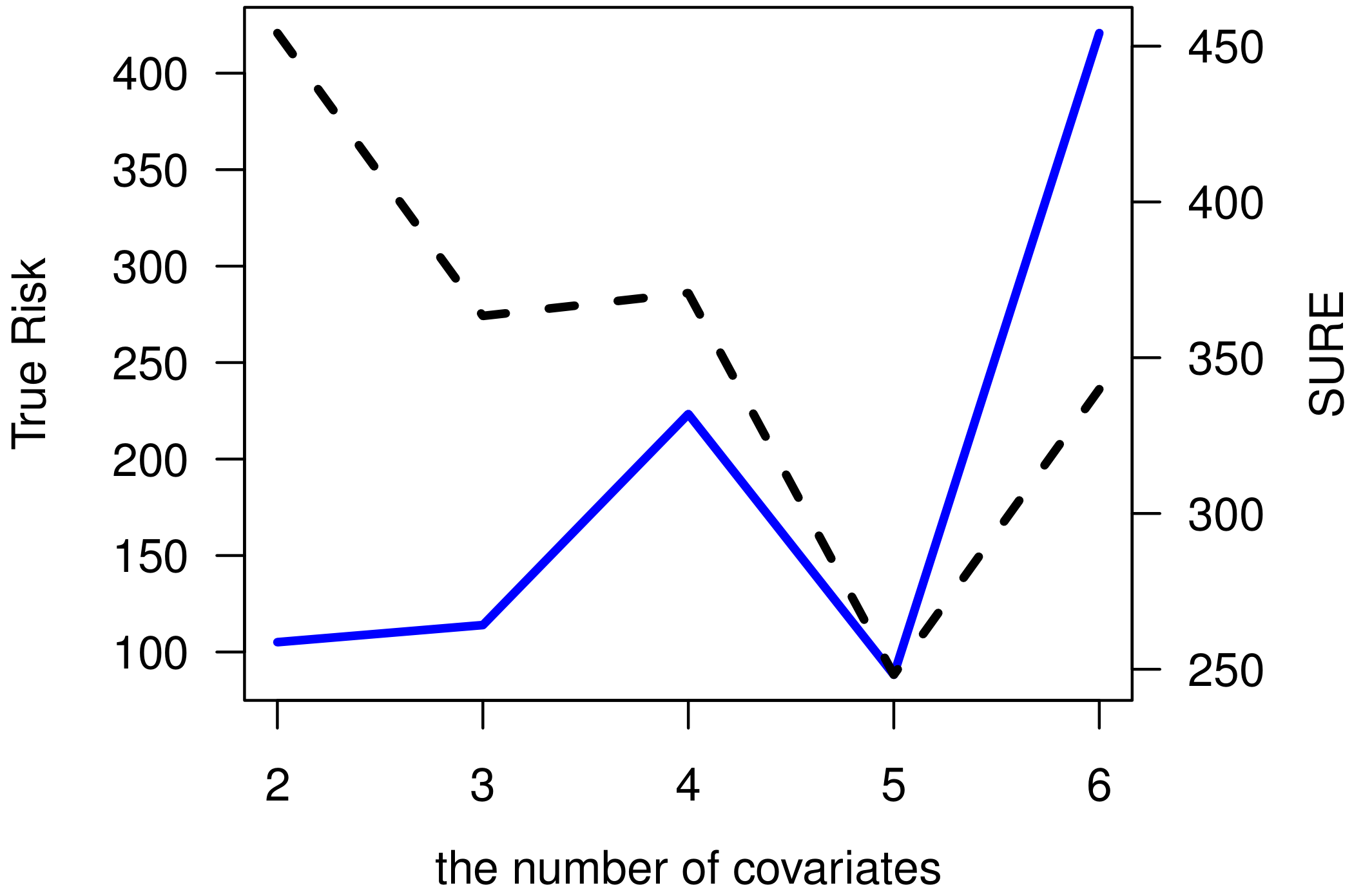
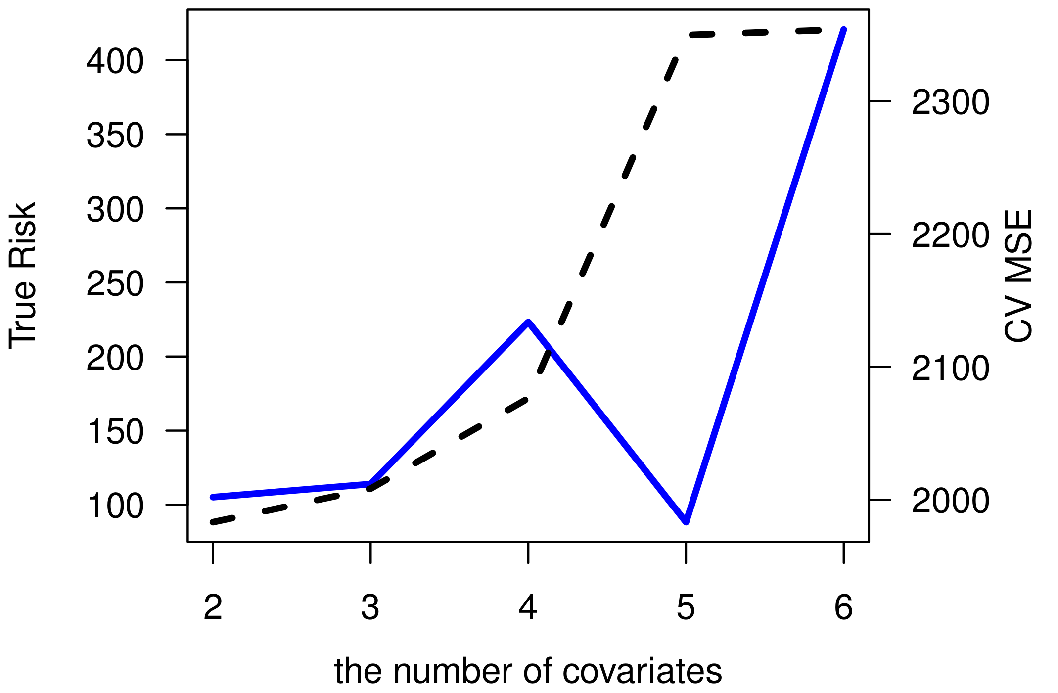
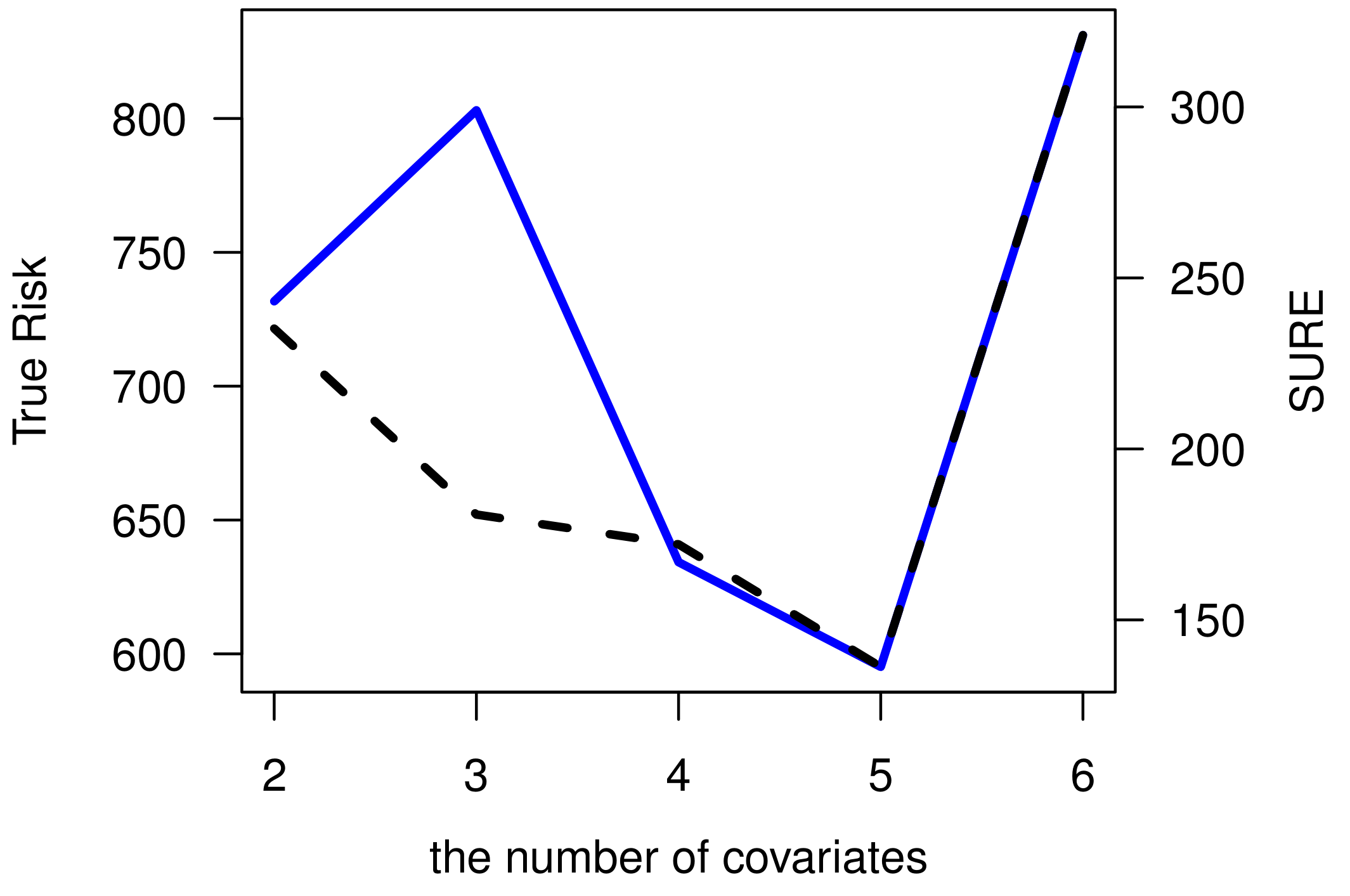
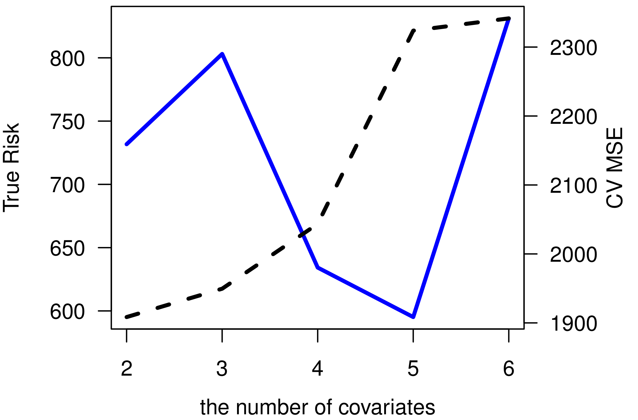
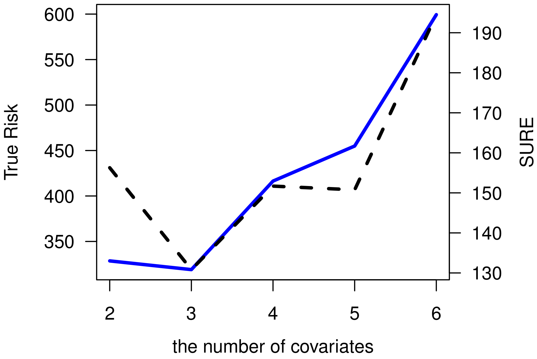
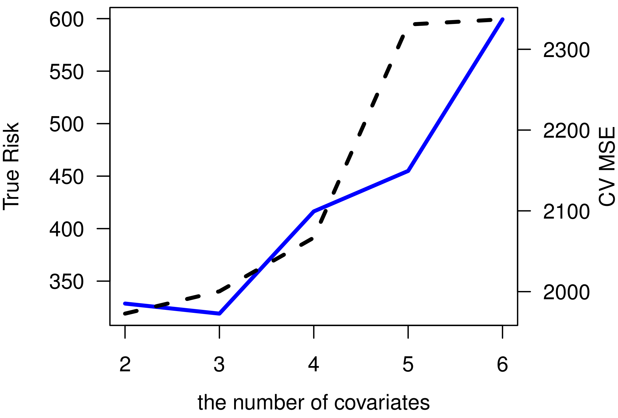
Figure 14: Illustration of covariate selection for the California Proposition 99 data. Covariates are selected by forward stepwise search. We produce risk v.s. $\lambda$ (black dashed curves), SURE v.s. $\lambda$ (blue bold curve) on the LHS, CV-MSE v.s. $\lambda$ (blue bold curve) on the RHS. The three rows use Iowa, Maine, and Dakota as pseudo-treated units respectively.

Appendix C Simulation Details

We wish to reproduce the “degrees of freedom vs average number of active donors” plot for the factor model simulation. Note that we use factor model simulation with all Gaussian noise, and where the noise of the to-be-treated unit is drawn from the empirical distribution.

Omitting time and model fixed effects for simplicity, we consider

$$Y_{t}^{*}=\psi_{t}^{T}L_{1},\ t=1,...,T,$$ (28)

$$X_{it}^{*}=\psi_{t}^{T}L_{i},\ i=2,...,p,\ t=1,...,T,$$ (29)

and

$$Y_{t}=Y_{t}^{*}+U_{1t},\ t=1,...,T,$$ (30)

$$X_{it}=X_{it}^{*}+U_{it},\ i=2,...,p,\ t=1,...,T.$$ (31)

First consider the Gaussian factor model with

$$E\left[\psi_{t}\right]=0,\ E\left[\psi_{t}\psi_{t}^{T}\right]=I,\ E\left[\mathbf{U}_{t}\mathbf{U}_{t}^{T}\right]=\Sigma,$$

where $\Sigma$ is assumed to be diagonal. Specifically, we assume that

$$\left(\begin{array}[]{c}Y_{t}\\ X_{t}\end{array}\right)\sim N\left(0,\mathbf{L}\mathbf{L}^{T}+\Sigma\right).$$

Note that

$$E\left[\left.Y_{t}\right|X_{it}\right]=E\left[\left.Y_{t}^{*}\right|X_{it}\right]$$

and

$$\left(\begin{array}[]{c}Y_{t}^{*}\\ X_{t}\end{array}\right)\sim N\left(0,\mathbf{L}\mathbf{L}^{T}+\left(\begin{array}[]{cc}0&0\\ 0&\Sigma_{X}\end{array}\right)\right).$$

Specifically, we can compute $Y_{t}$ as in (30) with both the Gaussian errors and the empirical distribution errors $U_{1t}$, and still compute the conditional expectation in closed form.

In particular, we can draw from the model (28)-(31) with Gaussian errors.

Alternatively, we can draw $Y_{it}$ as

$$Y_{t}\leftarrow E\left[\left.Y_{t}\right|X_{it}\right]+\hat{\varepsilon}_{1(t)},$$

where $\hat{\varepsilon}_{1(t)}$ is drawn from the empirical distribution of innovations, $\hat{\varepsilon}_{1t}=Y_{t}-E\left[\left.Y_{t}\right|X_{it}\right],\forall t$. We may sample the residuals using the block or stationary bootstrap to preserve serial correlation, although the method does not assume away serial dependence and we are therefore not concerned about assessing robustness in that respect.

With the closed form you can compute $\frac{1}{\sigma_{Y}^{2}}\sum_{t}Cov\left(\left.Y_{t},\hat{Y}_{t}\right|\mathbf{X}_{t}\right)$, the true df on the y-axis. The x-axis value is $df\left(\mathbf{X}\hat{\beta}_{\mathrm{pen}}\right)=\left(1+\lambda\right)(E|\mathcal{A}|-1)$.

References

- Abadie (\APACyear2021) \APACinsertmetastarabadie2021using{APACrefauthors}Abadie, A. \APACrefYearMonthDay2021. \BBOQ\APACrefatitleUsing synthetic controls: Feasibility, data requirements, and methodological aspects Using synthetic controls: Feasibility, data requirements, and methodological aspects.\BBCQ \APACjournalVolNumPagesJournal of Economic Literature592391–425. \PrintBackRefs\CurrentBib
- Abadie \BOthers. (\APACyear2010) \APACinsertmetastarabadie2010synthetic{APACrefauthors}Abadie, A., Diamond, A.\BCBL \BBA Hainmueller, J. \APACrefYearMonthDay2010. \BBOQ\APACrefatitleSynthetic control methods for comparative case studies: Estimating the effect of California’s tobacco control program Synthetic control methods for comparative case studies: Estimating the effect of california’s tobacco control program.\BBCQ \APACjournalVolNumPagesJournal of the American statistical Association105490493–505. \PrintBackRefs\CurrentBib
- Abadie \BOthers. (\APACyear2015) \APACinsertmetastarabadie2015comparative{APACrefauthors}Abadie, A., Diamond, A.\BCBL \BBA Hainmueller, J. \APACrefYearMonthDay2015. \BBOQ\APACrefatitleComparative politics and the synthetic control method Comparative politics and the synthetic control method.\BBCQ \APACjournalVolNumPagesAmerican Journal of Political Science592495–510. \PrintBackRefs\CurrentBib
- Abadie \BBA Gardeazabal (\APACyear2003) \APACinsertmetastarabadie2003economic{APACrefauthors}Abadie, A.\BCBT \BBA Gardeazabal, J. \APACrefYearMonthDay2003. \BBOQ\APACrefatitleThe economic costs of conflict: A case study of the Basque Country The economic costs of conflict: A case study of the basque country.\BBCQ \APACjournalVolNumPagesAmerican economic review931113–132. \PrintBackRefs\CurrentBib
- Abadie \BBA L’Hour (\APACyear2021) \APACinsertmetastarabadie2021penalized{APACrefauthors}Abadie, A.\BCBT \BBA L’Hour, J. \APACrefYearMonthDay2021. \BBOQ\APACrefatitleA penalized synthetic control estimator for disaggregated data A penalized synthetic control estimator for disaggregated data.\BBCQ \APACjournalVolNumPagesJournal of the American Statistical Associationjust-accepted1–34. \PrintBackRefs\CurrentBib
- Bai \BBA Ng (\APACyear2002) \APACinsertmetastarbai2002determining{APACrefauthors}Bai, J.\BCBT \BBA Ng, S. \APACrefYearMonthDay2002. \BBOQ\APACrefatitleDetermining the number of factors in approximate factor models Determining the number of factors in approximate factor models.\BBCQ \APACjournalVolNumPagesEconometrica701191–221. \PrintBackRefs\CurrentBib
- Ben-Michael \BOthers. (\APACyear2021) \APACinsertmetastarben2021augmented{APACrefauthors}Ben-Michael, E., Feller, A.\BCBL \BBA Rothstein, J. \APACrefYearMonthDay2021. \BBOQ\APACrefatitleThe augmented synthetic control method The augmented synthetic control method.\BBCQ \APACjournalVolNumPagesJournal of the American Statistical Associationjust-accepted1–34. \PrintBackRefs\CurrentBib
- Bifulco \BOthers. (\APACyear2017) \APACinsertmetastarbifulco2017using{APACrefauthors}Bifulco, R., Rubenstein, R.\BCBL \BBA Sohn, H. \APACrefYearMonthDay2017. \BBOQ\APACrefatitleUsing synthetic controls to evaluate the effect of unique interventions: The case of Say Yes to Education Using synthetic controls to evaluate the effect of unique interventions: The case of say yes to education.\BBCQ \APACjournalVolNumPagesEvaluation review416593–619. \PrintBackRefs\CurrentBib
- Billmeier \BBA Nannicini (\APACyear2013) \APACinsertmetastarbillmeier2013assessing{APACrefauthors}Billmeier, A.\BCBT \BBA Nannicini, T. \APACrefYearMonthDay2013. \BBOQ\APACrefatitleAssessing economic liberalization episodes: A synthetic control approach Assessing economic liberalization episodes: A synthetic control approach.\BBCQ \APACjournalVolNumPagesReview of Economics and Statistics953983–1001. \PrintBackRefs\CurrentBib
- Bohn \BOthers. (\APACyear2014) \APACinsertmetastarbohn2014did{APACrefauthors}Bohn, S., Lofstrom, M.\BCBL \BBA Raphael, S. \APACrefYearMonthDay2014. \BBOQ\APACrefatitleDid the 2007 Legal Arizona Workers Act reduce the state’s unauthorized immigrant population? Did the 2007 legal arizona workers act reduce the state’s unauthorized immigrant population?\BBCQ \APACjournalVolNumPagesReview of Economics and Statistics962258–269. \PrintBackRefs\CurrentBib
- Boyd \BBA Vandenberghe (\APACyear2018) \APACinsertmetastarboyd2018introduction{APACrefauthors}Boyd, S.\BCBT \BBA Vandenberghe, L. \APACrefYear2018. \APACrefbtitleIntroduction to applied linear algebra: vectors, matrices, and least squares Introduction to applied linear algebra: vectors, matrices, and least squares. \APACaddressPublisherCambridge university press. \PrintBackRefs\CurrentBib
- Breusch \BBA Pagan (\APACyear1979) \APACinsertmetastarbreusch1979simple{APACrefauthors}Breusch, T\BPBIS.\BCBT \BBA Pagan, A\BPBIR. \APACrefYearMonthDay1979. \BBOQ\APACrefatitleA simple test for heteroscedasticity and random coefficient variation A simple test for heteroscedasticity and random coefficient variation.\BBCQ \APACjournalVolNumPagesEconometrica: Journal of the econometric society1287–1294. \PrintBackRefs\CurrentBib
- Buaphim \BOthers. (\APACyear2018) \APACinsertmetastarbuaphim2018some{APACrefauthors}Buaphim, N., Onsaard, K., So-ngoen, P.\BCBL \BBA Rungratgasame, T. \APACrefYearMonthDay2018. \BBOQ\APACrefatitleSome reviews on ranks of upper triangular block matrices over a skew field Some reviews on ranks of upper triangular block matrices over a skew field.\BBCQ \BIn \APACrefbtitleInternational Mathematical Forum International mathematical forum (\BVOL 13, \BPGS 559–566). \PrintBackRefs\CurrentBib
- Candes \BOthers. (\APACyear2013) \APACinsertmetastarcandes2013unbiased{APACrefauthors}Candes, E\BPBIJ., Sing-Long, C\BPBIA.\BCBL \BBA Trzasko, J\BPBID. \APACrefYearMonthDay2013. \BBOQ\APACrefatitleUnbiased risk estimates for singular value thresholding and spectral estimators Unbiased risk estimates for singular value thresholding and spectral estimators.\BBCQ \APACjournalVolNumPagesIEEE transactions on signal processing61194643–4657. \PrintBackRefs\CurrentBib
- Cattaneo \BOthers. (\APACyear2021) \APACinsertmetastarcattaneo2021prediction{APACrefauthors}Cattaneo, M\BPBID., Feng, Y.\BCBL \BBA Titiunik, R. \APACrefYearMonthDay2021. \BBOQ\APACrefatitlePrediction intervals for synthetic control methods Prediction intervals for synthetic control methods.\BBCQ \APACjournalVolNumPagesJournal of the American Statistical Association1165361865–1880. \PrintBackRefs\CurrentBib
- Cavallo \BOthers. (\APACyear2013) \APACinsertmetastarcavallo2013catastrophic{APACrefauthors}Cavallo, E., Galiani, S., Noy, I.\BCBL \BBA Pantano, J. \APACrefYearMonthDay2013. \BBOQ\APACrefatitleCatastrophic natural disasters and economic growth Catastrophic natural disasters and economic growth.\BBCQ \APACjournalVolNumPagesReview of Economics and Statistics9551549–1561. \PrintBackRefs\CurrentBib
- Chen \BOthers. (\APACyear2020) \APACinsertmetastarchen2020degrees{APACrefauthors}Chen, X., Lin, Q.\BCBL \BBA Sen, B. \APACrefYearMonthDay2020. \BBOQ\APACrefatitleOn degrees of freedom of projection estimators with applications to multivariate nonparametric regression On degrees of freedom of projection estimators with applications to multivariate nonparametric regression.\BBCQ \APACjournalVolNumPagesJournal of the American Statistical Association115529173–186. \PrintBackRefs\CurrentBib
- Chernozhukov \BOthers. (\APACyear2018) \APACinsertmetastarchernozhukov2018t{APACrefauthors}Chernozhukov, V., Wuthrich, K.\BCBL \BBA Zhu, Y. \APACrefYearMonthDay2018. \BBOQ\APACrefatitleA -test for synthetic controls A -test for synthetic controls.\BBCQ \APACjournalVolNumPagesarXiv preprint arXiv:1812.10820. \PrintBackRefs\CurrentBib
- Chetverikov \BOthers. (\APACyear2021) \APACinsertmetastarchetverikov2021cross{APACrefauthors}Chetverikov, D., Liao, Z.\BCBL \BBA Chernozhukov, V. \APACrefYearMonthDay2021. \BBOQ\APACrefatitleOn cross-validated lasso in high dimensions On cross-validated lasso in high dimensions.\BBCQ \APACjournalVolNumPagesThe Annals of Statistics4931300–1317. \PrintBackRefs\CurrentBib
- Claeskens \BBA Hjort (\APACyear2008) \APACinsertmetastarclaeskens2008model{APACrefauthors}Claeskens, G.\BCBT \BBA Hjort, N\BPBIL. \APACrefYearMonthDay2008. \BBOQ\APACrefatitleModel selection and model averaging Model selection and model averaging.\BBCQ \APACjournalVolNumPagesCambridge Books. \PrintBackRefs\CurrentBib
- Daljord \BOthers. (\APACyear2021) \APACinsertmetastardaljord2021black{APACrefauthors}Daljord, Ø., Pouliot, G., Xiao, J.\BCBL \BBA Hu, M. \APACrefYearMonthDay2021. \BBOQ\APACrefatitleThe Black Market for Beijing License Plates The black market for beijing license plates.\BBCQ \APACjournalVolNumPagesarXiv preprint arXiv:2105.00517. \PrintBackRefs\CurrentBib
- Deledalle \BOthers. (\APACyear2012) \APACinsertmetastardeledalle2012risk{APACrefauthors}Deledalle, C\BHBIA., Vaiter, S., Peyré, G., Fadili, J.\BCBL \BBA Dossal, C. \APACrefYearMonthDay2012. \BBOQ\APACrefatitleRisk estimation for matrix recovery with spectral regularization Risk estimation for matrix recovery with spectral regularization.\BBCQ \APACjournalVolNumPagesarXiv preprint arXiv:1205.1482. \PrintBackRefs\CurrentBib
- Doudchenko \BBA Imbens (\APACyear2016) \APACinsertmetastardoudchenko2016balancing{APACrefauthors}Doudchenko, N.\BCBT \BBA Imbens, G\BPBIW. \APACrefYearMonthDay2016. \APACrefbtitleBalancing, regression, difference-in-differences and synthetic control methods: A synthesis Balancing, regression, difference-in-differences and synthetic control methods: A synthesis \APACbVolEdTR\BTR. \APACaddressInstitutionNational Bureau of Economic Research. \PrintBackRefs\CurrentBib
- Dutta \BBA Dempe (\APACyear2006) \APACinsertmetastardutta2006bilevel{APACrefauthors}Dutta, J.\BCBT \BBA Dempe, S. \APACrefYearMonthDay2006. \BBOQ\APACrefatitleBilevel programming with convex lower level problems Bilevel programming with convex lower level problems.\BBCQ \BIn \APACrefbtitleOptimization with multivalued mappings Optimization with multivalued mappings (\BPGS 51–71). \APACaddressPublisherSpringer. \PrintBackRefs\CurrentBib
- Efron (\APACyear2004) \APACinsertmetastarefron2004estimation{APACrefauthors}Efron, B. \APACrefYearMonthDay2004. \BBOQ\APACrefatitleThe estimation of prediction error: covariance penalties and cross-validation The estimation of prediction error: covariance penalties and cross-validation.\BBCQ \APACjournalVolNumPagesJournal of the American Statistical Association99467619–632. \PrintBackRefs\CurrentBib
- Ferman \BBA Pinto (\APACyear2021) \APACinsertmetastarferman2019synthetic{APACrefauthors}Ferman, B.\BCBT \BBA Pinto, C. \APACrefYearMonthDay2021. \BBOQ\APACrefatitleSynthetic controls with imperfect pre-treatment fit Synthetic controls with imperfect pre-treatment fit.\BBCQ \APACjournalVolNumPagesarXiv preprint arXiv:1911.08521. \PrintBackRefs\CurrentBib
- Friedman \BOthers. (\APACyear2001) \APACinsertmetastarfriedman2001elements{APACrefauthors}Friedman, J., Hastie, T.\BCBL \BBA Tibshirani, R. \APACrefYear2001. \APACrefbtitleThe elements of statistical learning The elements of statistical learning (\BVOL 1) (\BNUM 10). \APACaddressPublisherSpringer series in statistics New York. \PrintBackRefs\CurrentBib
- Hastie \BBA Tibshirani (\APACyear1990) \APACinsertmetastarhastie1990generalized{APACrefauthors}Hastie, T.\BCBT \BBA Tibshirani, R. \APACrefYear1990. \APACrefbtitleGeneralized Additive Models Generalized additive models (\BVOL 43). \APACaddressPublisherCRC Press. \PrintBackRefs\CurrentBib
- Heersink \BOthers. (\APACyear2017) \APACinsertmetastarheersink2017disasters{APACrefauthors}Heersink, B., Peterson, B\BPBID.\BCBL \BBA Jenkins, J\BPBIA. \APACrefYearMonthDay2017. \BBOQ\APACrefatitleDisasters and elections: Estimating the net effect of damage and relief in historical perspective Disasters and elections: Estimating the net effect of damage and relief in historical perspective.\BBCQ \APACjournalVolNumPagesPolitical Analysis252260–268. \PrintBackRefs\CurrentBib
- Kato (\APACyear2009) \APACinsertmetastarkato2009degrees{APACrefauthors}Kato, K. \APACrefYearMonthDay2009. \BBOQ\APACrefatitleOn the degrees of freedom in shrinkage estimation On the degrees of freedom in shrinkage estimation.\BBCQ \APACjournalVolNumPagesJournal of Multivariate Analysis10071338–1352. \PrintBackRefs\CurrentBib
- Kellogg \BOthers. (\APACyear2021) \APACinsertmetastarkellogg2020combining{APACrefauthors}Kellogg, M., Mogstad, M., Pouliot, G\BPBIA.\BCBL \BBA Torgovitsky, A. \APACrefYearMonthDay2021. \BBOQ\APACrefatitleCombining matching and synthetic control to trade off biases from extrapolation and interpolation Combining matching and synthetic control to trade off biases from extrapolation and interpolation.\BBCQ \APACjournalVolNumPagesJournal of the American Statistical Associationjust-accepted1–30. \PrintBackRefs\CurrentBib
- Li (\APACyear2018) \APACinsertmetastarli2018better{APACrefauthors}Li, S. \APACrefYearMonthDay2018. \BBOQ\APACrefatitleBetter lucky than rich? Welfare analysis of automobile licence allocations in Beijing and Shanghai Better lucky than rich? welfare analysis of automobile licence allocations in beijing and shanghai.\BBCQ \APACjournalVolNumPagesThe Review of Economic Studies8542389–2428. \PrintBackRefs\CurrentBib
- Liu (\APACyear1994) \APACinsertmetastarliu1994siegel{APACrefauthors}Liu, J\BPBIS. \APACrefYearMonthDay1994. \BBOQ\APACrefatitleSiegel’s formula via Stein’s identities Siegel’s formula via stein’s identities.\BBCQ \APACjournalVolNumPagesStatistics & Probability Letters213247–251. \PrintBackRefs\CurrentBib
- Mazumder \BBA Weng (\APACyear2020) \APACinsertmetastarmazumder2020computing{APACrefauthors}Mazumder, R.\BCBT \BBA Weng, H. \APACrefYearMonthDay2020. \BBOQ\APACrefatitleComputing the degrees of freedom of rank-regularized estimators and cousins Computing the degrees of freedom of rank-regularized estimators and cousins.\BBCQ \APACjournalVolNumPagesElectronic Journal of Statistics1411348–1385. \PrintBackRefs\CurrentBib
- Meyer \BBA Woodroofe (\APACyear2000) \APACinsertmetastarmeyer2000degrees{APACrefauthors}Meyer, M.\BCBT \BBA Woodroofe, M. \APACrefYearMonthDay2000. \BBOQ\APACrefatitleOn the degrees of freedom in shape-restricted regression On the degrees of freedom in shape-restricted regression.\BBCQ \APACjournalVolNumPagesThe annals of Statistics2841083–1104. \PrintBackRefs\CurrentBib
- Minami (\APACyear2020) \APACinsertmetastarminami2020degrees{APACrefauthors}Minami, K. \APACrefYearMonthDay2020. \BBOQ\APACrefatitleDegrees of freedom in submodular regularization: A computational perspective of Stein’s unbiased risk estimate Degrees of freedom in submodular regularization: A computational perspective of stein’s unbiased risk estimate.\BBCQ \APACjournalVolNumPagesJournal of Multivariate Analysis175104546. \PrintBackRefs\CurrentBib
- Mukherjee \BOthers. (\APACyear2015) \APACinsertmetastarmukherjee2015degrees{APACrefauthors}Mukherjee, A., Chen, K., Wang, N.\BCBL \BBA Zhu, J. \APACrefYearMonthDay2015. \BBOQ\APACrefatitleOn the degrees of freedom of reduced-rank estimators in multivariate regression On the degrees of freedom of reduced-rank estimators in multivariate regression.\BBCQ \APACjournalVolNumPagesBiometrika1022457–477. \PrintBackRefs\CurrentBib
- Peri \BBA Yasenov (\APACyear2019) \APACinsertmetastarperi2019labor{APACrefauthors}Peri, G.\BCBT \BBA Yasenov, V. \APACrefYearMonthDay2019. \BBOQ\APACrefatitleThe labor market effects of a refugee wave synthetic control method meets the mariel boatlift The labor market effects of a refugee wave synthetic control method meets the mariel boatlift.\BBCQ \APACjournalVolNumPagesJournal of Human Resources542267–309. \PrintBackRefs\CurrentBib
- Pieters \BOthers. (\APACyear2016) \APACinsertmetastarpieters2016effect{APACrefauthors}Pieters, H., Curzi, D., Olper, A.\BCBL \BBA Swinnen, J. \APACrefYearMonthDay2016. \BBOQ\APACrefatitleEffect of democratic reforms on child mortality: a synthetic control analysis Effect of democratic reforms on child mortality: a synthetic control analysis.\BBCQ \APACjournalVolNumPagesThe Lancet Global Health49e627–e632. \PrintBackRefs\CurrentBib
- Politis \BBA Romano (\APACyear1994) \APACinsertmetastarpolitis1994stationary{APACrefauthors}Politis, D\BPBIN.\BCBT \BBA Romano, J\BPBIP. \APACrefYearMonthDay1994. \BBOQ\APACrefatitleThe stationary bootstrap The stationary bootstrap.\BBCQ \APACjournalVolNumPagesJournal of the American Statistical association894281303–1313. \PrintBackRefs\CurrentBib
- Rao \BBA Toutenburg (\APACyear1995) \APACinsertmetastarrao1995linear{APACrefauthors}Rao, C\BPBIR.\BCBT \BBA Toutenburg, H. \APACrefYearMonthDay1995. \BBOQ\APACrefatitleLinear models Linear models.\BBCQ \BIn \APACrefbtitleLinear models Linear models (\BPGS 3–18). \APACaddressPublisherSpringer. \PrintBackRefs\CurrentBib
- Stein (\APACyear1981) \APACinsertmetastarstein1981estimation{APACrefauthors}Stein, C\BPBIM. \APACrefYearMonthDay1981. \BBOQ\APACrefatitleEstimation of the mean of a multivariate normal distribution Estimation of the mean of a multivariate normal distribution.\BBCQ \APACjournalVolNumPagesThe annals of Statistics1135–1151. \PrintBackRefs\CurrentBib
- Tibshirani \BBA Taylor (\APACyear2012) \APACinsertmetastartibshirani2012degrees{APACrefauthors}Tibshirani, R.\BCBT \BBA Taylor, J. \APACrefYearMonthDay2012. \BBOQ\APACrefatitleDegrees of freedom in lasso problems Degrees of freedom in lasso problems.\BBCQ \APACjournalVolNumPagesThe Annals of Statistics4021198–1232. \PrintBackRefs\CurrentBib
- Tibshirani \BBA Wasserman (\APACyear2015) \APACinsertmetastartibshirani2015stein{APACrefauthors}Tibshirani, R.\BCBT \BBA Wasserman, L. \APACrefYearMonthDay2015. \BBOQ\APACrefatitleStein’s unbiased risk estimate Stein’s unbiased risk estimate.\BBCQ \APACjournalVolNumPagesCourse notes from Statistical Machine Learning1–12. \PrintBackRefs\CurrentBib
- White (\APACyear1980) \APACinsertmetastarwhite1980heteroskedasticity{APACrefauthors}White, H. \APACrefYearMonthDay1980. \BBOQ\APACrefatitleA heteroskedasticity-consistent covariance matrix estimator and a direct test for heteroskedasticity A heteroskedasticity-consistent covariance matrix estimator and a direct test for heteroskedasticity.\BBCQ \APACjournalVolNumPagesEconometrica: journal of the Econometric Society817–838. \PrintBackRefs\CurrentBib
- Xu (\APACyear2017) \APACinsertmetastarxu2017generalized{APACrefauthors}Xu, Y. \APACrefYearMonthDay2017. \BBOQ\APACrefatitleGeneralized synthetic control method: Causal inference with interactive fixed effects models Generalized synthetic control method: Causal inference with interactive fixed effects models.\BBCQ \APACjournalVolNumPagesPolitical Analysis25157–76. \PrintBackRefs\CurrentBib
- Zou \BOthers. (\APACyear2007) \APACinsertmetastarzou2007degrees{APACrefauthors}Zou, H., Hastie, T.\BCBL \BBA Tibshirani, R. \APACrefYearMonthDay2007. \BBOQ\APACrefatitleOn the “degrees of freedom” of the lasso On the “degrees of freedom” of the lasso.\BBCQ \APACjournalVolNumPagesThe Annals of Statistics3552173–2192. \PrintBackRefs\CurrentBib