Efficient inverse $Z$-transform and pricing barrier and lookback options with discrete monitoring. II

Abstract.

We prove a simple general formula for the expectations of a function of a random walk and its running extremum, which is more convenient for applications than general formulas in the first version of the paper. The derivation of explicit formulas in applications significantly simplifies. Under additional conditions, we derive analytical formulas using the inverse $Z$-transform, Fourier/Laplace inversion and Wiener-Hopf factorization, and discuss efficient numerical methods for realization of these formulas. As applications, the cumulative probability distribution function of the process and its running maximum and the price of the option to exchange the maximum of a stock price for a power of the price are calculated. The most efficient numerical methods use a new efficient numerical realization of the inverse $Z$-transform, sinh-acceleration technique and simplified trapezoid rule. The program in Matlab running on a Mac with moderate characteristics achieves the precision E-10 and better in several dozen of milliseconds, and E-14 - in a fraction of a isecond.

Key words: $Z$-transform, extrema of a random walk, lookback options, barrier options, discrete monitoring, Lévy processes, Fourier transform, Hilbert transform, Fast Fourier transform, fast Hilbert transform, trapezoid rule, sinh-acceleration

MSC2020 codes: 60-08,42A38,42B10,44A10,65R10,65G51,91G20,91G60

1. Introduction

Let $Y,Y_{j},j=1,2\ldots,$ be i.i.d. ${\mathbb{R}}$-valued random variables on a probability space $({\Omega},{\mathcal{B}},{\mathbb{Q}})$, and ${\mathbb{E}}$ the expectation operator under ${\mathbb{Q}}$. For $x\in{\mathbb{R}}$, $X_{n}=x+Y_{1}+\cdots+Y_{n},n=0,1,2,\ldots,$ is a random walk on ${\mathbb{R}}$ starting at $x$. In applications to finance, typically, $Y$ is an increment of a Lévy process, and the random walk appears implicitly when either a continuous time Lévy model is approximated or options with discrete monitoring are priced. In the present paper, we derive a general formula and efficient numerical procedure for evaluation of expectations of a random walk and its extremum. The formula and procedure can be applied to lookback, single barrier options and single barrier options with lookback features. The method of the paper can be used as the main basic block to price double-barrier options with lookback features and discrete monitoring, and American options with barrier/lookback features.

Let ${\bar{X}}_{n}=\max_{0\leq m\leq n}X_{m}$ and ${\underline{X}}_{n}=\min_{0\leq m\leq t}X_{m}$ be the supremum and infimum processes (defined path-wise, a.s.); $X_{0}={\bar{X}}_{0}={\underline{X}}_{0}=0$. For a measurable function $f$, consider $V(f;n;x_{1},x_{2})={\mathbb{E}}[f(x_{1}+X_{n},\max\{x_{2},x_{1}+{\bar{X}}_{n}\})].$ At the first step, as in [28], where barrier options with discrete monitoring in the Brownian motion model are priced, we make the discrete Laplace transform ($Z$-transform) of the series $\vec{V}:=\{V_{n}\}_{n=0}^{\infty}:=\{V(f;n;x_{1},x_{2})\}_{n=0}^{\infty}$. For our purposes, it is convenient to use the equivalent transformation

(1.1) $${\tilde{V}}(z)=\sum_{n=0}^{+\infty}z^{n}V_{n}.$$

If $f$ is uniformly bounded, the series $\vec{V}$ is uniformly bounded as well, hence, ${\tilde{V}}(z)$ is analytic in the open unit disc, and $\vec{V}$ can be recovered using the residue theorem: for any $R<1$,

(1.2) $$V_{n}=\frac{1}{2\pi i}\int_{|z|=R}z^{-n-1}{\tilde{V}}(z)dz.$$

The standard and popular approximation to the integral on the RHS is the trapezoid rule. However, if $n$ is very large, then the trapezoid rule becomes very inefficient as we discuss in Sect. 2 and illustrate with numerical examples in Sect. 5. The first contribution of the paper is a new efficient method for a numerical evaluation the integral on the RHS of (1.2). The idea is to deform the contour of integration $\{z=Re^{i\varphi}\ |\ -\pi<\varphi<\pi\}$ into a contour of the form ${\mathcal{L}}_{L;\sigma_{\ell},b_{\ell},\omega_{\ell}}=\chi_{L;\sigma_{\ell},b_{\ell},\omega_{\ell}}({\mathbb{R}})$, where the conformal map $\chi_{L;\sigma_{\ell},b_{\ell},\omega_{\ell}}$ is defined by

(1.3) $$\chi_{L;\sigma_{\ell},b_{\ell},\omega_{\ell}}(y)=\sigma_{\ell}+ib_{\ell}\sinh(i\omega_{\ell}+y),$$

$b_{\ell}>0$, $\sigma_{\ell}\in{\mathbb{R}}$ and $\omega_{\ell}\in(-\pi/2,\pi/2)$. The deformation is possible under natural conditions on the domain of analyticity of ${\tilde{V}}$; these conditions are satisfied in applications that we consider. After the deformation and corresponding change of variables, the simplified trapezoid rule is applied. The resulting procedure is faster and more accurate than the trapezoid rule. We hope that a new efficient numerical method for the evaluation of the inverse $Z$-transform (1.2) is of a general interest.

The second contribution of the paper is a general formula for ${\tilde{V}}(f;z;x_{1},x_{2})$ in terms of the expected present value operators (EPV-operators) ${\mathcal{E}}^{\pm}_{q}$ under the supremum and infimum processes introduced in [11, 14, 15]. The formula and its proof are essentially identical to the ones in [21] for Lévy processes, only the definitions of the operators ${\mathcal{E}}^{\pm}_{q}$ change. In the case of random walks, the action of ${\mathcal{E}}^{\pm}_{q}$ is defined as follows. For $q\in(0,1)$, let $T_{q}$ be a random variable with the distribution ${\mathbb{E}}[T_{q}=n]=(1-q)q^{n}$, independent of $X$, and let $u$ be a bounded measurable function. Then ${\mathcal{E}^{+}_{q}}u(x)={\mathbb{E}}[u(x+{\bar{X}}_{T_{q}})]$ and ${\mathcal{E}^{-}_{q}}u(x)={\mathbb{E}}[u(x+{\underline{X}}_{T_{q}})]$. The formula is in Sect. 3.2. In applications, the payoff function $f$ may increase exponentially at infinity. Hence, in order that the expectation be finite, one or even two tails of the probability distribution of $Y$ must decay exponentially at infinity. We formulate and prove a general theorem for the case of exponentially increasing payoff functions.

In Section 3.3, we use the Fourier transform and the equalities ${\mathcal{E}}^{\pm}_{q}e^{ix\xi}=\phi^{\pm}_{q}(\xi)e^{ix\xi}$, where $\phi^{\pm}_{q}(\xi)$ are the Wiener-Hopf factors, to realize the formula derived in Section 3.2 as a sum of 1D-3D integrals; formulas for the Wiener-Hopf factors are in Sect. 3.1. As applications of the general theorems, in Section 3.4, we derive explicit formulas for the cumulative distribution function (cpdf) of random walk and its maximum, and for the option to exchange $e^{{\bar{X}}_{T}}$ for a power $e^{\beta X_{T}}$.

If one of the tails of the pdf of $Y$ exponentially decays at infinity, the characteristic function $\Phi(\xi)={\mathbb{E}}[e^{i\xi Y}]$ of $Y$ and the Wiener-Hopf factors admit analytic continuation to a strip around or adjacent to the real axis. This property allows one to use the useful property of the infinite trapezoid rule, namely, the exponential decay of the discretization error as a function of $1/\zeta$, where $\zeta$ is the step of the infinite trapezoid rule. However, in many cases of interest such as pricing options with daily monitoring and/or Lévy processes close to the Variance Gamma process, the integrand decays too slowly at infinity, therefore, the number of terms in the simplified trapezoid rule necessary to satisfy even a moderate error tolerance can be huge. Fortunately, in all popular models, $\Phi(\xi)$ admits analytic continuation to a cone around the real axis and exponentially decays as $\xi\to\infty$ in the cone (the only exception is the Variance Gamma model; the rate of decay is a polynomial one). See [22] for the explicit calculation of the coni of analyticity in popular models. Therefore, the sinh-acceleration technique used in [18] to price European options and applied in [20, 19, 23] to price barrier options and evaluate special functions and the coefficients in BPROJ method respectively can be applied to greatly decrease the sizes of grids and the CPU time needed to satisfy the desired error tolerance. The changes of variables must be in a certain agreement as in [16, 42, 21]. Note that the deformation (1.3) and the corresponding change of variables constitute an example of the application of the sinh-acceleration technique. We show that, in some cases, one of the integrals (either outer or inner one) has to be calculated using a less efficient family of sub-polynomial deformations introduced and used in [19]. Numerical examples are in Section 5. We demonstrate that the method based on the sinh-acceleration for the inverse $Z$-transform can achieve the accuracy of the order of E-14 and better using Matlab and Mac with moderate characteristics, in a second or fraction of a second, and the precision of the order of E-10 in 20-30 msec., for options of maturity in the range $T=0.25-15Y$. In all cases, the arrays are of a moderate size. In particular, the number of points used for the $Z$-transform inversion is several dozens in all cases. If the trapezoid rule is used, the size of arrays and CPU time increase with the maturity, and, for maturity $T=15$, approximately 3,000 points are needed, and the CPU time is several times larger. We also compare the results in the case of the continuous monitoring using the methods developed in [21] and demonstrate that in the case of daily monitoring, the relative differences are rather small even for $T=15Y$.

There is a huge body of the literature devoted to pricing options with barrier and/or lookback features, and a number of different methods have been applied. The methods that are conceptually close to the method of the paper are the ones that use the fast inverse Fourier transform, fast convolution or fast Hilbert transform. In Section 6, we review several popular methods and explain why these methods are computationally more expensive than the method of the present paper and cannot achieve the precision demonstrated in Section 5. We also summarize the results of the paper and outline several extensions of the method of the paper. We relegate to Appendix A several technicalities. Figures and tables are in Appendix B.

2. Efficient inverse $Z$-transform

2.1. Trapezoid rule

Let a sequence $\vec{V}=(V)_{n=0}^{\infty}$ and $A>0$ satisfy

(2.1) $$H(\vec{V},A):=\sum_{n=0}^{\infty}|V_{n}|A^{n}<+\infty.$$

Then, for any $z\in{\mathcal{D}}(0,A):=\{z\in{\mathbb{C}}\ |\ |z|\leq A\}$, the series (1.1) converges and defines the function analytic in ${\mathcal{D}}(0,A)$ (meaning: analytic in the open domain $\{|z|<1/A\}$ and continuous up to the boundary). Hence, $V_{n}$ can be recovered using the Cauchy residue theorem. Explicitly, for any $R<A$, (1.2) holds. Changing the variable $z\mapsto zR$, and introducing $h(z)(=h(R,z))=(zR)^{-n}{\tilde{V}}(zR)$, we obtain

(2.2) $$V_{n}=\frac{1}{2\pi i}\int_{|z|=1}h(z)\frac{dz}{z},\ n=0,1,2,\ldots$$

Usually, one evaluates the RHS of (2.2), denote it $I(h)$, using the trapezoid rule:

(2.3) $$T_{M}(h)=(1/M)\sum_{k=0}^{M-1}h(\zeta_{M}^{k}),$$

where $M>1$ is an integer, and $\zeta_{M}=\exp(2\pi i/M)$ is the standard primitive $M$-th root of unity. For $0<a<b$, denote ${\mathcal{D}}_{(a,b)}:=\{z\ |\ a<|z|<b\}$. Since $R<A$, $h(z)$ is analytic in the annulus ${\mathcal{D}}_{(1/\rho,\rho)}$. The Hardy norm of $h$ is

$$\|h\|_{{\mathcal{D}}_{(1/\rho,\rho)}}=\frac{1}{2\pi i}\int_{|z|=1/\rho}|h(z)|\frac{dz}{z}+\frac{1}{2\pi i}\int_{|z|=\rho}|h(z)|\frac{dz}{z}.$$

The error bound is well-known; for completeness, we give the proof in Sect. A.1.

Theorem 2.1.

Let $h$ be analytic in ${\mathcal{D}}_{(1/\rho,\rho)}$, where $\rho>1$. The error of the trapezoid approximation admits the bound

(2.4) $$|T_{M}(h)-I(h)|\leq\frac{\rho^{-M}}{1-\rho^{-M}}\|h\|_{{\mathcal{D}}_{(1/\rho,\rho)}}.$$

If $V_{n}$ are real, then $\overline{h(z)}=h(\bar{z})$, hence, we can choose an odd $M=2M_{0}+1$ and obtain

(2.5) $$T_{M}(h)=(2/M)\operatorname{\rm Re}\sum_{k=0}^{M-1}h(\zeta_{M}^{k})(1-\delta_{k0}/2).$$

2.2. Sinh-acceleration

Let there exist $\gamma\in(0,\pi)$ such that ${\tilde{V}}$ admits analytic continuation to a domain of the form ${\mathcal{U}}(R,\rho,\gamma)=({\mathcal{D}}(R/\rho,R\rho)-({\mathcal{C}}_{\gamma}\cup\{0\}))\setminus{\mathcal{D}}(0,R/\rho)$, where ${\mathcal{C}}_{\gamma}=\{z\ |\ \mathrm{arg}\,z\in(-\gamma,\gamma)\}$, and let there exist $C_{{\tilde{V}}}>0$ and $a_{{\tilde{V}}}<n$ such that

(2.6) $$|{\tilde{V}}(z)|\leq C_{{\tilde{V}}}|z|^{a_{{\tilde{V}}}},\ z\in{\mathcal{U}}(R,\rho,\gamma).$$

Then we can deform the contour of integration $\{z=Re^{i\varphi}\ |\ -\pi<\varphi<\pi\}$ in (1.2) into a contour of the form ${\mathcal{L}}_{L;\sigma_{\ell},b_{\ell},\omega_{\ell}}=\chi_{L;\sigma_{\ell},b_{\ell},\omega_{\ell}}({\mathbb{R}})$, where the conformal map $\chi_{L;\sigma_{\ell},b_{\ell},\omega_{\ell}}$ is defined by (1.3). After the transformation, we make the corresponding change of variables and reduce to the integral over ${\mathbb{R}}$:

(2.7) $$V_{n}=\int_{{\mathbb{R}}}\frac{b_{\ell}}{2\pi}\chi_{L;\sigma_{\ell},b_{\ell},\omega_{\ell}}(y)^{-n-1}\cosh(i\omega_{\ell}+y){\tilde{V}}(\chi_{L;\sigma_{\ell},b_{\ell},\omega_{\ell}}(y))dy,$$

denote by $f_{n}(y)$ be the integrand on the RHS of (2.7), and apply the infinite trapezoid rule

(2.8) $$V_{n}\approx\zeta_{\ell}\sum_{j\in{\mathbb{Z}}}f_{n}(j\zeta_{\ell}).$$

An error bound is easy to derive because the function $f_{n}$ is analytic in a strip $S_{(-d,d)}:=\{\xi\ |\operatorname{\rm Im}\xi\in(-d,d)\}$, where $d>0$ depends on the domain of analyticity of ${\tilde{V}}$ and the choice of the parameters $\sigma_{\ell},\omega_{\ell},b_{\ell}$, and (2.6) holds. With an appropriate choice of the parameters $\omega_{\ell},\sigma_{\ell},b_{\ell}$ and $d$, $\lim_{R\to\pm\infty}\int_{-d}^{d}|f_{n}(is+R)|ds=0,$ and

(2.9) $$H(f_{n},d):=\|f_{n}\|_{H^{1}(S_{(-d,d)})}:=\lim_{s\downarrow-d}\int_{\mathbb{R}}|g(is+t)|dt+\lim_{s\uparrow d}\int_{\mathbb{R}}|g(is+t)|dt<\infty.$$

We write $f_{n}\in H^{1}(S_{(-d,d)})$. The following key lemma is proved in [47] using the heavy machinery of sinc-functions. A simple proof (analogous to the proof of Theorem 2.1) can be found in [41].

Lemma 2.2 ([47], Thm.3.2.1).

For $f_{n}\in H^{1}(S_{(-d,d)})$, the error of the infinite trapezoid rule admits an upper bound

(2.10) $${\rm Err}_{\rm disc}\leq H(f_{n},d)\frac{\exp[-2\pi d/\zeta]}{1-\exp[-2\pi d/\zeta]}.$$

Once an approximate bound $H_{\mathrm{appr.}}(f_{n},d)$ for $H(f_{n},d)$ is derived, it becomes possible to satisfy the desired error tolerance with a good accuracy letting

(2.11) $$\zeta_{\ell}=2\pi d\ln(H_{\mathrm{appr.}}(f_{n},d)/\epsilon).$$

Since $f_{n}(y)$ decays as $((b/2)e^{|y|})^{-n-1}$ as $y\to\pm\infty$, it is straightforward to choose the truncation of the infinite sum on the RHS of (2.8):

(2.12) $$V_{n}\approx\zeta_{\ell}\sum_{|j|\leq M_{0}}f_{n}(j\zeta_{\ell})$$

to satisfy the given error tolerance. A good approximation to $\Lambda:=M_{0}\zeta$ is

(2.13) $$\Lambda=\frac{1}{n-a_{{\tilde{V}}}}\ln\frac{C_{{\tilde{V}}}}{\epsilon}-\ln\frac{b}{2},$$

where $C_{{\tilde{V}}}$ and $a_{{\tilde{V}}}$ are from (2.6). If $V_{n}$ are real, then $\overline{h(z)}=h(\bar{z})$, and, therefore, we can replace (2.12) with

(2.14) $$V_{n}\approx 2\zeta_{\ell}\operatorname{\rm Re}\sum_{j=0}^{M_{0}}f_{n}(j\zeta_{\ell})(1-\delta_{j0}/2).$$

The complexity of the numerical scheme is of the order of $(n+1-a_{{\tilde{V}}})^{-1}\ln(H(f_{n},d)/\epsilon)\ln(1/\epsilon)$. If double precision arithmetic is used, then the deformation must be chosen so that the $f(j\zeta)$ are not very large. Furthermore, the image of the strip $S_{(-d,d)}$ under the map $\chi_{L;\sigma_{\ell},b_{\ell},\omega_{\ell}}$ has non-empty intersection with the unit disc, hence, if the parameters of the deformation are fixed, and $n$ increases, then $H(f_{n},d)$ increases as $B^{n+1}$, where $B>1$ depends on the chosen deformation. Therefore, the problem of an accurate bound for the Hardy norm and choice of $\zeta_{\ell}$ becomes non-trivial. This difficulty can be alleviated if $\gamma>\pi/4$, better, $\gamma>\pi/2$ (we will see that in applications to pricing options with discrete monitoring, $\gamma>\pi/2$) choosing $n$-dependent parameters of the deformation. Case I. $\gamma\in(\pi/4,\pi/2]$ or $\gamma>\pi/2$ but $\gamma-\pi/2$ is very small. We set $\omega_{\ell}=3\pi/8-\gamma/2$, and take $d_{\ell}\in(0,(\gamma-\pi/4)/2)$, e.g., $d_{\ell}=0.95\cdot(\gamma-\pi/4)/2$. Next,

1. if $A>1$ and $A-1$ is not very small, we find $b_{\ell}$ and $\sigma_{\ell}$ solving the system $1=\sigma_{\ell}-b_{\ell}\sin(\omega_{\ell}+d_{\ell}),A=\sigma_{\ell}-b_{\ell}\sin(\omega_{\ell}-d_{\ell})$. A fairly safe upper bound for $H(f_{n},d)$ is $H_{\mathrm{appr.}}(f_{n},d)=C_{{\tilde{V}}}\max\{1,B\}$, where $B$ is the supremum of $y$ s.t. $\chi_{L;\sigma_{\ell},b_{\ell},\omega_{\ell}}(i(\omega_{\ell}+d_{\ell})+y)\in{\mathcal{D}}(0,1)$;

2. if $A$ is close to 1 (this is the case when the time interval between the monitoring dates is small), we set $R=1-5/n$, and find $b_{\ell}$ and $\sigma_{\ell}$ solving the system $R=\sigma_{\ell}-b_{\ell}\sin(\omega_{\ell}+d_{\ell}),1=\sigma_{\ell}-b_{\ell}\sin(\omega_{\ell}-d_{\ell})$. A fairly safe upper bound for $H(f_{n},d)$ is $H_{\mathrm{appr.}}(f_{n},d)=C_{{\tilde{V}}}R^{-n-1}B$, where $B$ is the supremum of $y$ s.t. $\chi_{L;\sigma_{\ell},b_{\ell},\omega_{\ell}}(i(\omega_{\ell}+d_{\ell})+y)\in{\mathcal{D}}(0,1)$. If $\gamma$ is close to $\pi/4$, it is necessary to replace $R^{-n-1}$ with $\sup_{0\leq y\leq B}|\chi_{L;\sigma_{\ell},b_{\ell},\omega_{\ell}}(i(\omega_{\ell}+d_{\ell})+y)|^{-n-1}$.

Case II. $\gamma\in(\pi/2,\pi)$, and $\gamma-\pi/2$ is not very small. We choose $\omega_{\ell}=(\pi/2-\gamma)/2$, and $d_{\ell}\in(0,|\omega_{\ell}|)$, e.g., $d_{\ell}=0.95|\omega_{\ell}|$. Next,

1. if $A>1$ and $A-1$ is not very small, we find $b_{\ell}$ and $\sigma_{\ell}$ solving the system $1=\sigma_{\ell}-b_{\ell}\sin(\omega_{\ell}-d_{\ell}),A=\sigma_{\ell}-b_{\ell}\sin(\omega_{\ell}+d_{\ell})$. A fairly safe upper bound for $H(f_{n},d)$ is $H_{\mathrm{appr.}}(f_{n},d)=C_{{\tilde{V}}}\max\{1,B\}$, where $B$ is the supremum of $y$ s.t. $\chi_{L;\sigma_{\ell},b_{\ell},\omega_{\ell}}(i(\omega_{\ell}-d_{\ell})+y)\in{\mathcal{D}}(0,1)$;

2. if $A$ is close to 1, we set $R=1-5/n$, and find $b_{\ell}$ and $\sigma_{\ell}$ solving the system $R=\sigma_{\ell}-b_{\ell}\sin(\omega_{\ell}-d_{\ell}),1=\sigma_{\ell}-b_{\ell}\sin(\omega_{\ell}+d_{\ell})$. A fairly safe upper bound for $H(f_{n},d)$ is $H_{\mathrm{appr.}}(f_{n},d)=C_{{\tilde{V}}}R^{-n-1}B$, where $B$ is the supremum of $y$ s.t. $\chi_{L;\sigma_{\ell},b_{\ell},\omega_{\ell}}(i(\omega_{\ell}-d_{\ell})+y)\in{\mathcal{D}}(0,1)$.

Case III. If $A<1$ and $1-A$ is not small, we suggest to make the change of variables $z=Az^{\prime}$, follow Steps I and II, and choose the step $\zeta_{\ell}$ and the number of terms $M_{0}$ using the error tolerance $\epsilon A^{-n-1+a_{{\tilde{V}}}}$.

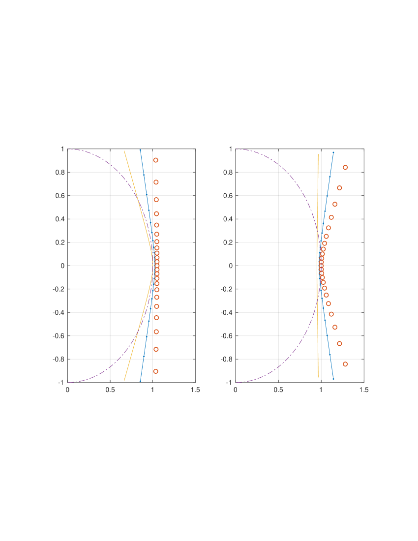
Figure 1. Cases I(i) (left panel) and II(ii) (right panel). Dots: the unit circle. Dots-dashes, circles and solid lines: the curves $\chi_{L;\sigma_{\ell},b_{\ell},\omega_{\ell}}(i\omega_{\ell}+{\mathbb{R}})$, $\chi_{L;\sigma_{\ell},b_{\ell},\omega_{\ell}}(i(\omega_{\ell}+d_{\ell})+{\mathbb{R}})$, $\chi_{L;\sigma_{\ell},b_{\ell},\omega_{\ell}}(i(\omega_{\ell}-d_{\ell})+{\mathbb{R}})$.

See Fig. 1 for illustrations of Cases I(i) and II(ii).

3. Expectations of functions of random walk and its extremum

3.1. The Wiener-Hopf factorization

Let ${\mathcal{E}_{q}}$ be the EPV-operator under $X$ defined by $u(x)={\mathbb{E}}[u(X_{T_{q}})]$; the EPV operators ${\mathcal{E}}^{\pm}_{q}$ are defined in the introduction. We realize the EPV operators ${\mathcal{E}_{q}}$ and ${\mathcal{E}}^{\pm}_{q}$ as pseudo-differential operators (PDO) with the symbols $(1-q)/(1-q\Phi(\xi))$ and $\phi^{\pm}_{q}(\xi)$, where ${\phi^{+}_{q}}(\xi)={\mathbb{E}}[e^{i\xi{\bar{X}}_{T_{q}}}]$ and ${\phi^{-}_{q}}(\xi)={\mathbb{E}}[e^{i\xi{\underline{X}}_{T_{q}}}]$ are the Wiener-Hopf factors. We use the following key result valid for random walks on ${\mathbb{R}}$ and Lévy processes $X$ on ${\mathbb{R}}$ [31, 30]; in the latter case, $T_{q}$ is an exponentially distributed random variable on mean $q$, independent of $X$. See [3, 45, 46] for the references to the literature on the Wiener-Hopf factorization and various fluctuation identities.

Lemma 3.1.

Let $X$ and $T_{q}$ be as above. Then

1. the random variables ${\bar{X}}_{T_{q}}$ and $X_{T_{q}}-{\bar{X}}_{T_{q}}$ are independent; and

2. the random variables ${\underline{X}}_{T_{q}}$ and $X_{T_{q}}-{\bar{X}}_{T_{q}}$ are identical in law.

(By symmetry, the statements (a), (b) are valid with ${\bar{X}}$ and ${\underline{X}}$ interchanged). The two basic forms of the Wiener-Hopf factorization (both immediate from Lemma 3.1) are

(3.1) $${\mathcal{E}_{q}}={\mathcal{E}^{+}_{q}}{\mathcal{E}^{-}_{q}}={\mathcal{E}^{-}_{q}}{\mathcal{E}^{+}_{q}},$$

and

(3.2) $$\frac{1-q}{1-q\Phi(\xi)}={\phi^{+}_{q}}(\xi){\phi^{-}_{q}}(\xi).$$

Explicit analytic formulas for the Wiener-Hopf factors are easy to derive if at least one tail of the pdf of $Y$ decays exponentially, equivalently, $\Phi$ admits analytic continuation to a strip $S_{[\mu_{-},\mu_{+}]}$, where $\mu_{-}\leq 0\leq\mu_{+}$, and $\mu_{-}<\mu_{+}$. The formulas for and the properties of the Wiener-Hopf factors are well-known, see, e.g., [3, 11, 15]; we include a short proof in Sect. A.2.

Proposition 3.2.

Let $\Phi$ admit analytic continuation to a strip $S_{[\lambda_{-},\lambda_{+}]}$, where $\lambda_{-}\leq 0\leq\lambda_{+}$, and $\lambda_{-}<\lambda_{+}$. Then, for any $q\in(0,1)$,

1. there exist $\mu_{-}\geq\lambda_{-}$ and $\mu_{+}\leq\lambda_{+}$ s.t. $\mu_{-}<\mu_{+}$, and $c>0$ such that

   (3.3) $$\operatorname{\rm Re}(1-q\Phi(\xi))\geq c,\quad\xi\in S_{[\mu_{-},\mu_{+}]}.$$

2. Furthermore, for any $\xi$ in the half-plane $\{\operatorname{\rm Im}\xi>\mu_{-}\}$ and any $\omega_{-}\in[\mu_{-},\operatorname{\rm Im}\xi)$,

   (3.4) $${\phi^{+}_{q}}(\xi) = \exp\left[-\frac{1}{2\pi i}\int_{\operatorname{\rm Im}\xi=\omega_{-}}\frac{\xi\ln((1-q)/(1-q\Phi(\eta)))}{\eta(\xi-\eta)}d\eta\right],$$

   and for any $\xi$ in the half-plane $\{\operatorname{\rm Im}\xi<\mu_{+}\}$ and any $\omega_{+}\in(\operatorname{\rm Im}\xi,\mu_{+}]$,

   (3.5) $${\phi^{-}_{q}}(\xi) = \exp\left[\frac{1}{2\pi i}\int_{\operatorname{\rm Im}\xi=\omega_{+}}\frac{\xi\ln((1-q)/(1-q\Phi(\eta)))}{\eta(\xi-\eta)}d\eta\right];$$

3. Let let there exist $\delta>0$ such that $\Phi(\xi)=O(|\xi|^{-\delta})$ as $(S_{[\mu_{-},\mu_{+}]}\ni)\xi\to\infty$. Then $\phi^{\pm}_{q}(\xi)=c^{\pm}_{q}+\phi^{\pm,\pm}_{q}(\xi)$, where $\phi^{\pm,\pm}_{q}(\xi)=O(|\xi|^{-\delta+\epsilon})$ as $(S_{[\mu_{-}+\epsilon,\mu_{+}-\epsilon]}\ni)\xi\to\infty$, for any $\epsilon>0$, and $c^{\pm}_{q}$ are given by

   (3.6) $$c^{\pm}_{q}=\exp\left[\pm\frac{1}{2\pi i}\int_{\operatorname{\rm Im}\eta=\omega_{\mp}}\frac{\ln(1-q\Phi(\eta))}{\eta}\right],$$

   where $\omega_{-}\in(\mu_{-},0)$ and $\omega_{+}\in(0,\mu_{+})$. If $\mu_{-}=0$, then $c^{+}_{q}=(1-q)/c^{-}_{q}$, and if $\mu_{+}=0$, then $c^{-}_{q}=(1-q)/c^{+}_{q}$.

Example 3.3.

Let $\Phi(\xi)=e^{-\bar{\Delta}\psi(\xi)}$, where $\bar{\Delta}>0$ is the time interval between the monitoring dates, and $\psi$ the characteristic exponent of a Lévy process. Then, in the Variance Gamma model, $\Phi(\xi)=O(|\xi|^{-\bar{\Delta}\delta})$, where $\delta>0$ depends on the parameters of the process, and in all other popular models, $\Phi(\xi)=O(e^{-\bar{\Delta}c_{\infty}|\xi|^{\nu}})$, where $c_{\infty}>0$ and $\nu\in(0,2]$ (see [22]).

The integrands on the RHS’ of the formulas for the Wiener-Hopf factors above decay slowly at infinity, hence, very long grids are necessary to calculate the Wiener-Hopf factors. If $\Phi$ admits analytic continuation to the union of a strip and cone containing or adjacent to the real line, then the Wiener-Hopf factors can be calculated with almost machine precision using appropriate conformal deformations of the lines of integration on the RHS’ of (3.4)-(3.5). See Sect. 4.2.

3.2. Main theorems

Let $X$, $q$ and $T_{q}$ be as in the introduction. Let $f$ be measurable and uniformly bounded on $U_{+}:=\{(x_{1},x_{2})\ |\ x_{2}\geq 0,x_{1}\leq x_{2}\}$. Consider $V(f;n;x_{1},x_{2})={\mathbb{E}}[f(x_{1}+X_{n},\max\{x_{2},x_{1}+{\bar{X}}_{n}\})].$ We write the (modified) $Z$-transform (1.1) in the form

(3.7) $$(1-q){\tilde{V}}(q)={\mathbb{E}}[f(x_{1}+X_{T_{q}},\max\{x_{2},x_{1}+{\bar{X}}_{T_{q}}\})].$$

Notationally, the Wiener-Hopf factorization technique for random walks is identical to the Wiener-Hopf factorization technique for Lévy processes. See, e.g., [11, 15]. The following theorem is a counterpart of [21, Thm. 3.1] for Lévy processes; $I$ denotes the identity operator, $f_{+}$ is the extension of $f$ to ${\mathbb{R}}^{2}$ by zero, and $\Delta$ is the diagonal map: $\Delta(x)=(x,x)$.

Theorem 3.4.

Let $X$ be a Lévy process on ${\mathbb{R}}$, $q>0$, and let $f:U_{+}\to{\mathbb{R}}$ be a measurable and uniformly bounded function s.t. $(({\mathcal{E}^{-}_{q}}\otimes I)f)\circ\Delta:{\mathbb{R}}\to{\mathbb{R}}$ is measurable. Then

1. for any $x_{1}\leq x_{2}$,

   (3.8) $$(1-q){\tilde{V}}(f;q;x_{1},x_{2}) = (({\mathcal{E}_{q}}\otimes I)f_{+})(x_{1},x_{2})+({\mathcal{E}^{+}_{q}}w(f;q,\cdot,x_{2}))(x_{1}),$$

   where

   (3.9) $$w(f;q,y,x_{2})={\bf 1}_{[x_{2},+\infty)}(y)((({\mathcal{E}^{-}_{q}}\otimes I)f_{+})(y,y)-(({\mathcal{E}^{-}_{q}}\otimes I)f_{+})(y,x_{2}));$$

2. as a function of $q$, ${\tilde{V}}(f,q;x_{1},x_{2})$ admits analytic continuation to the open unit disc.

Proof.

We use Lemma 3.1. By definition, part (a) amounts to the statement that the probability distribution of the ${\mathbb{R}}^{2}$-valued random variable $({\bar{X}}_{T_{q}},X_{T_{q}}-{\bar{X}}_{T_{q}})$ is equal to the product (in the sense of “product measure”) of the distribution of ${\bar{X}}_{T_{q}}$ and the distribution of $X_{T_{q}}-{\bar{X}}_{T_{q}}$. Hence, we can apply Fubini’s theorem. For $x_{1}\leq x_{2}$, we have

$${\mathbb{E}}[f_{+}(x_{1}+X_{T_{q}},\max\{x_{2},x_{1}+{\bar{X}}_{T_{q}}\})]$$

$$= {\mathbb{E}}[f_{+}(x_{1}+X_{T_{q}}-{\bar{X}}_{T_{q}}+{\bar{X}}_{T_{q}},\max\{x_{2},x_{1}+{\bar{X}}_{T_{q}}\})]$$

$$= {\mathbb{E}}[(({\mathcal{E}^{-}_{q}}\otimes I)f_{+})(x_{1}+{\bar{X}}_{T_{q}},\max\{x_{2},x_{1}+{\bar{X}}_{T_{q}}\})]$$

$$= {\mathbb{E}}[(({\mathcal{E}^{-}_{q}}\otimes I)f_{+})(x_{1}+{\bar{X}}_{T_{q}},x_{2})]$$

$$+{\mathbb{E}}[{\bf 1}_{x_{1}+\bar{X}_{T_{q}}\geq x_{2}}((({\mathcal{E}^{-}_{q}}\otimes I)f_{+})(x_{1}+{\bar{X}}_{T_{q}},x_{1}+{\bar{X}}_{T_{q}})-(({\mathcal{E}^{-}_{q}}\otimes I)f_{+})(x_{1}+{\bar{X}}_{T_{q}},x_{2}))].$$

Using (3.1), we write the first term on the rightmost side as $(({\mathcal{E}_{q}}\otimes I)f_{+})(x_{1},x_{2})$, and finish the proof of (i). As operators acting in the space of bounded measurable functions, ${\mathcal{E}}^{\pm}_{q}$ admit analytic continuation w.r.t. $q$ to the open unit disc, which proves (ii).

∎

Remark 3.1.

The inverse $Z$-transform of $(1-q)^{-1}({\mathcal{E}_{q}}\otimes I)f_{+}(x_{1},x_{2})$ equals ${\mathbb{E}}[f(x_{1}+X_{T},x_{2})]$, and, therefore, can be easily calculated using the Fourier transform technique. Essentially, we have the price of the European option of maturity $T$, the riskless rate being 0, depending on $x_{2}$ as a parameter. Thus, the new element is the calculation of the second term on the RHS of (3.8). We calculate both terms in the same manner in order to facilitate the explanation of various blocks of our method.

In exponential Lévy models which are typically used in quantitative finance, payoff functions may increase exponentially, and options with discrete monitoring are typical situations where random walks appear implicitly. Hence, we consider the action of the EPV-operators in $L_{\infty}({\mathbb{R}};w)$, $L_{\infty}$- spaces with the weights $w(x)=e^{\gamma x}$, $\gamma\in[\mu_{-},\mu_{+}]$, and $w(x)=\min\{e^{\mu_{-}x},e^{\mu_{+}x}\}$, where $\mu_{-}\leq 0\leq\mu_{+},\mu_{-}<\mu_{+}$; the norm is defined by $\|u\|_{L_{\infty}({\mathbb{R}};w)}=\|wu\|_{L_{\infty}({\mathbb{R}})}$. The following theorem is the straightforward reformulation of Theorem 3.2 in [21], the condition $q+\psi(i\gamma)>0$ for the Lévy process being replaced with $1-q\Phi(i\gamma)>0$. The proof is the same.

Theorem 3.5.

Let a Lévy process $X$ on ${\mathbb{R}}$, function $f:U_{+}\to{\mathbb{R}}$ and $q\in(0,1)$ satisfy the following conditions

1. there exist $\mu_{-}\leq 0\leq\mu_{+}$ such that $\forall$ $\gamma\in[\mu_{-},\mu_{+}]$, ${\mathbb{E}}[e^{-\gamma Y}]<\infty$ and $1-q\Phi(i\gamma)>0$;

2. $f$ is a measurable function admitting the bound

   (3.10) $$|f(x_{1},x_{2})|\leq C(x_{2})e^{-\mu_{+}x_{1}},$$

   where $C(x_{2})$ is independent of $x_{1}\leq x_{2}$;

3. the function $(({\mathcal{E}^{-}_{q}}\otimes I)f)\circ\Delta$ is measurable and admits the bound

   (3.11) $$|(({\mathcal{E}^{-}_{q}}\otimes I)f)(x_{1},x_{1})|\leq Ce^{-\mu_{-}x_{1}},$$

   where $C$ is independent of $x_{1}\geq 0$.

Then the statements (i)-(iii) of Theorem 3.4 hold.

Remark 3.2.

Evaluating the RHS of (3.8), we will apply the Fourier transform and its inverse. If $f_{+}(x_{1},x_{2})$ is a piece-wise smooth function of the first argument so that the Fourier transform (w.r.t. the first argument) decays not slower than $|\xi|^{-1}$ at infinity, but $f_{+}(\cdot,x_{2})$ has points of discontinuity, then the composition of the Fourier transform and its inverse cannot recover $f_{+}(\cdot,x_{2})$ at the points of discontinuity. For instance, in the example of the joint cpdf, $f_{+}(x_{1},x_{2})={\bf 1}_{(-\infty,a_{1}]}(x_{1}){\bf 1}_{(-\infty,a_{2}]}(x_{2})$, where $a_{1}\leq a_{2}$, is dicontinuous at $x_{1}=a_{1}$ and $x_{2}=a_{2}$. Hence, we represent ${\mathcal{E}_{q}}$ in the form ${\mathcal{E}_{q}}=(1-q)I+(1-q)q\Phi(D)(1-q\Phi(D))^{-1}$, and calculate the first term on the RHS of (3.8) as follows:

(3.12) $$(({\mathcal{E}_{q}}\otimes I)f_{+})(x_{1},x_{2})=(1-q)f_{+}(x_{1},x_{2})+\frac{1}{2\pi}\int_{\operatorname{\rm Im}\xi_{1}=\omega}\frac{e^{ix_{1}\xi_{1}}(1-q)q\Phi(\xi_{1})}{1-q\Phi(\xi_{1})}\hat{(f_{+})}_{1}(\xi_{1},x_{2})d\xi_{1},$$

where $\widehat{(f_{+})}_{1}(\xi_{1},x_{2})={\mathcal{F}}_{x_{1}\to\xi_{1}}f_{+}(x_{1},x_{2})$ is the Fourier transform of $f_{+}$ w.r.t. the first argument, and admissible $\omega\in(\mu_{-},\mu_{+})$ depend on the rate of increase of $f(x_{1},x_{2})$ as $x_{1}\to-\infty$. In particular, if $f$ is uniformly bounded, then any $\omega\in(0,\mu_{+})$ is admissible. If $\widehat{(f_{+})}_{1}(\xi_{1},x_{2})=O(|\xi_{1}|^{-1})$ and $\Phi(\xi_{1})=O(|\xi_{1}|^{-\delta})$ as $\xi\to\infty$ along the line of integration, where $\delta>0$, then the integrand on the RHS of (3.12) is of class $L_{1}$, and the integral defines a function continuous in $x_{1}$.

Let $V(G;h;n;x)$ be the price of the barrier option with the payoff $G(X_{n})$ at maturity and no rebate if the barrier $h$ is crossed before or at time $n$; the rsikless rate is 0. Applying Theorem 3.5 and Remark 3.2, we obtain

Theorem 3.6.

Let a random walk $X$ on ${\mathbb{R}}$ and $q\in(0,1)$ satisfy condition (a) of Theorem 3.5, and let $G$ be a measurable function admitting the bound $|G(x)|\leq C(e^{-\mu_{+}x}+e^{-\mu_{-}x})$, where $C$ is independent of $x\in{\mathbb{R}}$. Then, for $x<h$,

(3.13) $${\tilde{V}}(G;h;q,x)=G(x)+(q\Phi(D)(1-q\Phi(D))^{-1}G)(x)-(1-q)^{-1}({\mathcal{E}^{+}_{q}}{\bf 1}_{[h,+\infty)}{\mathcal{E}^{-}_{q}}G)(x).$$

Remark 3.3.

The advantage of the representation (3.13) as compared to the equivalent formula

(3.14) $${\tilde{V}}(G;h;q,x)=(1-q)^{-1}({\mathcal{E}^{+}_{q}}{\bf 1}_{(-\infty,h)}{\mathcal{E}^{-}_{q}})G(x)$$

(see [15] for the references) is that if ${\hat{G}}(\xi)=O(|\xi|)^{-1}$ and $\Phi(\xi)=O(|\xi|^{-\delta})$ as $\xi\to\infty$ in a strip around or adjacent to the real axis, where $\delta>0$, then all the terms on the RHS of (3.13) bar the first one are Hölder continuous on $(-\infty,h)$, and numerical results are more accurate.

3.3. Fourier transform realization, the case $q\in(0,1)$

In this Subsection, $q\in(0,1)$ is fixed. The RHS’ of the formulas for the Wiener-Hopf factors and formulas that we derive below admit analytic continuation w.r.t. $q$ so that the inverse $Z$-transform can be applied. We use ${\mathcal{E}}^{\pm}_{q}=c^{\pm}_{q}I+{\mathcal{E}}^{\pm,\pm}_{q}$, where ${\mathcal{E}}^{\pm,\pm}_{q}=\phi^{\pm,\pm}_{q}(D)$, and the equality

$$w(f;q,x_{1},x_{2})={\bf 1}_{[x_{2},+\infty)}(x_{1})((({\mathcal{E}^{-}_{q}}\otimes I)f_{+})(x_{1},x_{1})-(({\mathcal{E}^{-}_{q}}\otimes I)f_{+})(x_{1},x_{2}))=0,\quad x_{1}\leq x_{2}.$$

to write the second term on the RHS of (3.8) as

(3.15) $$({\mathcal{E}^{+}_{q}}w(f;q,\cdot,x_{2}))(x_{1})=({\mathcal{E}}^{++}_{q}w(f;q,\cdot,x_{2}))(x_{1}),$$

and (3.9) as

(3.16) $$w(f;q,y,x_{2})=c^{-}_{q}w_{0}(y,x_{2})+w^{-}(f;q,y,x_{2}),$$

where $w_{0}(y,x_{2})={\bf 1}_{[x_{2},+\infty)}(y)(f_{+}(y,y)-f_{+}(y,x_{2}))$, and

(3.17) $$w^{-}(f;q,y,x_{2})={\bf 1}_{[x_{2},+\infty)}(y)((({\mathcal{E}}^{--}_{q}\otimes I)f_{+})(y,y)-(({\mathcal{E}}^{--}_{q}\otimes I)f_{+})(y,x_{2})).$$

Substituting (3.16) into (3.15), we obtain

(3.18) $$({\mathcal{E}^{+}_{q}}w(f;q,\cdot,x_{2}))(x_{1})=c^{-}_{q}(({\mathcal{E}}^{++}_{q}\otimes I)w_{0})(x_{1},x_{2})+(({\mathcal{E}}^{++}_{q}\otimes I)w^{-})(f;q,x_{1},x_{2}).$$

In order to derive explicit integral representations for the terms on the RHS of (3.18), we impose the following conditions, which can be relaxed:

1. condition (a) of Theorem 3.5 is satisfied;

2. there exist $\mu^{\prime}_{-},\mu^{\prime}_{+}\in(\mu_{-},\mu_{+})$, $\mu^{\prime}_{-}<\mu^{\prime}_{+}$ such that $f$ admits bounds

   (3.19) $$|f(x_{1},x_{2})| \leq C(x_{2})e^{-\mu^{\prime}_{+}x_{1}},\ x_{1}\leq x_{2},$$

   (3.20) $$|(({\mathcal{E}^{-}_{q}}\otimes I)f_{+})(x_{1},x_{1})| \leq Ce^{-\mu^{\prime}_{-}x_{1}},\ x_{1}\in{\mathbb{R}},$$

   where $C(x_{2})$ and $C$ are independent of $x_{1}\leq x_{2}$, and $x_{1}\in{\mathbb{R}}$, respectively;

3. for any $x_{2}$, there exists $C(x_{2})>0$ such that

   (3.21) $$|\widehat{(f_{+})}_{1}(\xi_{1},x_{2})| \leq C(x_{2})(1+|\xi_{1}|)^{-1},\quad\xi_{1}\in S_{[\mu^{\prime}_{+},\mu_{+}]},$$

   (3.22) $$|\widehat{(w_{0})}_{1}(\eta,x_{2})| \leq C(x_{2})(1+|\eta|)^{-1},\quad\eta\in S_{[\mu_{-},\mu^{\prime}_{-}]};$$

4. there exists $C>0$ such that for $\xi_{1}\in S_{[\mu^{\prime}_{+},\mu_{+}]}$ and $\xi_{2}\in S_{[\mu_{-},\mu^{\prime}_{-}]}$,

   (3.23) $$|\widehat{(f_{+})}(\xi_{1},\xi_{2})|\leq C(1+|\xi_{1}|)^{-1}(1+|\xi_{2}|)^{-1};$$

5. there exists $\delta>0$ such that $\Phi(\xi)=O(|\xi|^{-\delta})$ as $(S_{[\mu_{-},\mu_{+}]}\ni)\xi\to\infty$.

Theorem 3.7.

Let conditions (a)-(e) hold. Then, for any $\omega,\omega_{1},\omega_{2}$ and $\omega_{-}$ satisfying

(3.24) $$\omega,\omega_{1}\in(\mu^{\prime}_{+},\mu_{+}),\ \omega_{2}\in(\mu_{-},\mu^{\prime}_{-}),\ \omega_{-}\in(\mu_{-},\omega_{1}+\omega_{2}),$$

and $x_{1}\leq x_{2}$,

$${\tilde{V}}(f;q;x_{1},x_{2}) = f(x_{1},x_{2})+\frac{1}{2\pi}\int_{\operatorname{\rm Im}\xi_{1}=\omega}\frac{e^{ix_{1}\xi_{1}}q\Phi(\xi_{1})}{1-q\Phi(\xi_{1})}\hat{(f_{+})}_{1}(\xi_{1},x_{2})$$

$$+\frac{c^{-}_{q}}{2\pi(1-q)}\int_{\operatorname{\rm Im}\eta=\omega_{-}}e^{ix_{1}\eta}\phi^{++}_{q}(\eta)\widehat{(w_{0})}_{1}(\eta,x_{2})d\eta$$

$$+\frac{1}{2\pi(1-q)}\int_{\operatorname{\rm Im}\eta=\omega_{-}}e^{i(x_{1}-x_{2})\eta}\phi^{++}_{q}(\eta)\widehat{w^{-}_{0}}(f;q,\eta,x_{2})d\eta,$$

where $\widehat{w^{-}_{0}}(f;q,\eta,x_{2})$ is given by

$$\widehat{w^{-}_{0}}(f;q,\eta,x_{2})$$

$$= \frac{1}{2\pi}\int_{\operatorname{\rm Im}\xi_{1}=\omega_{1}}d\xi_{1}\,\frac{e^{ix_{2}\xi_{1}}}{i(\xi_{1}-\eta)}\phi^{--}_{q}(\xi_{1})(\widehat{f_{+}})_{1}(\xi_{1},x_{2})$$

$$+\frac{1}{(2\pi)^{2}}\int_{\operatorname{\rm Im}\xi_{1}=\omega_{1}}\int_{\operatorname{\rm Im}\xi_{2}=\omega_{2}}d\xi_{1}\,d\xi_{2}\,\frac{e^{ix_{2}(\xi_{1}+\xi_{2})}}{i(\eta-\xi_{1}-\xi_{2})}\phi^{--}_{q}(\xi_{1})(\widehat{f_{+}})(\xi_{1},\xi_{2}).$$

Proof.

Essentially, we repeat the proof of Theorem 4.1 in [21], with small necessary changes. We calculate the terms on the RHS of (3.8). The first two terms on the RHS of (3.7) follow from (3.12). Consider the third term. Since (3.22) holds and $\phi^{++}_{q}(\eta)=O(|\eta|^{-\delta_{1}})$ as $\eta\to\infty$ in the strip $S_{[\mu_{-},\mu_{+}]}$, where $\delta_{1}>0$, the integral

(3.27) $$({\mathcal{E}}^{++}_{q}w_{0}(\cdot,x_{2}))(x_{1})=\frac{1}{2\pi}\int_{\operatorname{\rm Im}\eta=\omega_{-}}e^{ix_{1}\eta}\phi^{++}_{q}(\eta)\widehat{(w_{0})}_{1}(\eta,x_{2})d\eta$$

is absolutely convergent. It remains to consider $({\mathcal{E}}^{++}_{q}w^{-}(f;q,\cdot,x_{2}))(x_{1})$. If $\operatorname{\rm Im}\eta=\omega_{-}$,

$$\widehat{w^{-}}(f;q,\eta,x_{2}) = -\int_{x_{2}}^{+\infty}dy\,e^{-iy\eta}\frac{1}{2\pi}\int_{\operatorname{\rm Im}\xi_{1}=\omega_{1}}d\xi_{1}\,e^{i\xi_{1}y}\phi^{--}_{q}(\xi_{1})(\widehat{f_{+}})_{1}(\xi_{1},x_{2})$$

$$+\int_{x_{2}}^{+\infty}dy\,e^{-iy\eta}\frac{1}{(2\pi)^{2}}\int_{\operatorname{\rm Im}\xi_{1}=\omega}\int_{\operatorname{\rm Im}\xi_{2}=\omega_{2}}d\xi_{1}\,d\xi_{2}\,e^{i(\xi_{1}+\xi_{2})y}\phi^{--}_{q}(\xi_{1})(\widehat{f_{+}})(\xi_{1},\xi_{2}).$$

We apply Fubini’s theorem to the first integral. The integral $\int_{x_{2}}^{+\infty}dy\,e^{i(-\eta+\xi_{1})y}=\frac{e^{ix_{2}(\xi_{1}-\eta)}}{i(\eta-\xi_{1})}$ converges absolutely since $-\omega_{-}+\omega_{1}>0$, and the repeated integral converges absolutely because $\phi^{--}_{q}(\xi)$ is uniformly bounded on the line of integration and (3.21) holds. Similarly, since $-\omega_{-}+\omega_{1}+\omega_{2}>0$, the integral $\int_{x_{2}}^{+\infty}dy\,e^{i(-\eta+\xi_{1}+\xi_{2})y}=e^{ix_{2}(\xi_{1}+\xi_{2}-\eta)}/(i(\eta-\xi_{1}-\xi_{2}))$ converges absolutely. Since (3.23) holds, $\phi^{--}_{q}(\xi)=O(|\xi_{1}|^{-\delta_{1}})$ as $\xi_{1}\to\infty$ along the line of integration, where $\delta_{1}>0$, and

(3.28) $$\int_{\mathbb{R}}\int_{\mathbb{R}}d\xi_{1}\,d\xi_{2}\,(1+|\xi_{1}+\xi_{2}|)^{-1}(1+|\xi_{1}|)^{-1-\delta_{1}}(1+|\xi_{2}|)^{-1}<\infty,$$

the Fubini’s theorem is applicable to the second integral as well. Thus,

(3.29) $$\widehat{w^{-}}(f;q,\eta,x_{2})=e^{-i\eta x_{2}}\widehat{w^{-}_{0}}(f;q,\eta,x_{2}),$$

where $\widehat{w^{-}_{0}}(f;q,\eta,x_{2})$ is given by (3.7), and we obtain the triple integral

(3.30) $$({\mathcal{E}}^{++}_{q}w^{-}(\cdot,x_{2})(x_{1})=\frac{1}{2\pi}\int_{\operatorname{\rm Im}\eta=\omega_{-}}e^{i(x_{1}-x_{2})\eta}\phi^{++}_{q}(\eta)\widehat{w^{-}_{0}}(f;q,\eta,x_{2})d\eta.$$

The integrand admits a bound via $Cg(\eta,\xi_{1},\xi_{2})$, where

$$g(\eta,\xi_{1},\xi_{2})=(1+|\eta|)^{-\delta_{1}}(1+|\eta-\xi_{1}-\xi_{2}|)^{-1}(1+|\xi_{1}|)^{-1-\delta_{1}}(1+|\xi_{2}|)^{-1}$$

is of class $L_{1}({\mathbb{R}}^{3})$ (see [21, Eq.(3.24)]). Substituting (3.12), (3.18), (3.27) and (3.30) into (3.8), we obtain (3.7).

∎

Remark 3.4.

In standard situations such as in the two examples that we consider below, the function $y\mapsto h(y)=({\mathcal{E}}^{--}_{q}\otimes I)f_{+}(y,y)-({\mathcal{E}}^{--}_{q}\otimes I)f_{+}(y,x_{2})$ is a linear combination of exponential functions (with the coefficients depending on $x_{2}$). Then $\widehat{w^{-}}(q;\eta,x_{2})$ can be calculated directly, the double integral on the RHS of (3.7) can be reduced to 1D integrals, and the condition (3.23) replaced with the condition on $h$ similar to (3.22). Analogous simplifications are possible in more involved cases when $h$ is a piece-wise exponential polynomial in $y$.

3.4. Two examples

3.4.1. Example I. The joint cpdf of $X_{n}$ and ${\bar{X}}_{n}$.

For $a_{1}\leq a_{2}$, and $x_{1}\leq x_{2}$, set $f(x_{1},x_{2})={\bf 1}_{(-\infty,\min\{a_{1},x_{2}\}]}(x_{1}){\bf 1}_{(-\infty,a_{2}]}(x_{2})$ and consider

$$V(f;n,x_{1},x_{2})={\mathbb{Q}}[x_{1}+X_{n}\leq a_{1},x_{2}+{\bar{X}}_{n}\leq a_{2}].$$

If $x_{2}>a_{2}$, then $V(f;n,x_{1},x_{2})=0$. Hence, we assume that $x_{2}\leq a_{2}$.

Theorem 3.8.

Let $q\in(0,1)$, $a_{1}\leq a_{2},x_{1}\leq x_{2}\leq a_{2}$, and let the following conditions hold:

1. there exist $\mu_{-}<0<\mu_{+}$ such that $\forall$ $\gamma\in[\mu_{-},\mu_{+}]$, ${\mathbb{E}}[e^{-\gamma Y}]<\infty$, and $1-q\Phi(i\gamma)>0$;

2. there exists $\delta>0$ such that $\Phi(\xi)=O(|\xi|^{-\delta})$ as $(S_{[\mu_{-},\mu_{+}]}\ni)\xi\to\infty$.

Then, for any $\mu_{-}<\omega_{-}<0<\omega_{1}<\mu_{+}$, and $\omega\in(0,\mu_{+})$,

$${\tilde{V}}(f;q,x_{1},x_{2})$$

$$= {\bf 1}_{(-\infty,a_{1}]}(x_{1})+\frac{1}{2\pi}\int_{\operatorname{\rm Im}\xi_{1}=\omega}\frac{e^{i(x_{1}-a_{1})\xi_{1}}q\Phi(\xi_{1})}{-i\xi_{1}(1-q\Phi(\xi_{1}))}d\xi_{1}$$

$$+\frac{1}{(2\pi)^{2}(1-q)}\int_{\operatorname{\rm Im}\eta=\omega_{-}}d\eta\,e^{i(x_{1}-a_{2})\eta}\phi^{++}_{q}(\eta)\int_{\operatorname{\rm Im}\xi_{1}=\omega_{1}}d\xi_{1}\,\frac{e^{i\xi_{1}(a_{2}-a_{1})}\phi^{--}_{q}(\xi_{1})}{\xi_{1}(\xi_{1}-\eta)}.$$

Proof.

We repeat the proof of Theorem 3.8 in [21] with small necessary modifications. We have $f_{+}(x_{1},x_{2})={\bf 1}_{(-\infty,a_{1}]}(x_{1}){\bf 1}_{(-\infty,a_{2}]}(x_{2}),$ therefore, for $x_{2}\leq a_{2}$,

$$w_{0}(y,x_{2}) = {\bf 1}_{[x_{2},+\infty)}(y){\bf 1}_{(-\infty,a_{1}]}(y)({\bf 1}_{(-\infty,a_{2}]}(y)-{\bf 1}_{(-\infty,a_{2}]}(x_{2}))$$

$$= -{\bf 1}_{[x_{2},+\infty)}(y){\bf 1}_{(-\infty,a_{1}]}(y){\bf 1}_{(a_{2},+\infty)}(y)=0,$$

hence, the third term on the RHS of (3.7) is 0. Next,

$$\widehat{(f_{+})}_{1}(\xi_{1},x_{2})={\bf 1}_{(-\infty,a_{2}]}(x_{2})\int_{-\infty}^{a_{1}}e^{-ix_{1}\xi_{1}}d\xi_{1}={\bf 1}_{(-\infty,a_{2}]}(x_{2})\frac{e^{-ia_{1}\xi_{1}}}{-i\xi_{1}}d\xi_{1}$$

is well-defined in the upper half-plane, and satisfies the bound (3.21) in any strip $S_{[\mu^{\prime}_{+},\mu_{+}]}$, where $\mu^{\prime}_{+}\in(0,\mu_{+})$. Thus, the first two terms on the RHS of (3.7) are the first terms on the RHS of (3.8). It remains to evaluate the double integral on the RHS of (3.7). As mentioned in Remark 3.4, in the present case, it is simpler to evaluate $w^{-}$, and then $\widehat{w^{-}}$, directly: for any $x_{2}\leq a_{2}$, $\omega_{1}\in(0,\mu_{+})$ and any $\eta\in\{\operatorname{\rm Im}\eta\in(\mu_{-},\omega_{1})\}$,

$$w^{-}(q,y,x_{2}) = {\bf 1}_{(x_{2},+\infty)}(y)({\mathcal{E}}^{--}_{q}{\bf 1}_{(-\infty,a_{1}]})(y)({\bf 1}_{(-\infty,a_{2}]}(y)-1)$$

$$= -{\bf 1}_{[a_{2},+\infty)}(y)({\mathcal{E}}^{--}_{q}{\bf 1}_{(-\infty,a_{1}]})(y)$$

$$= -{\bf 1}_{(a_{2},+\infty)}(y)\frac{1}{2\pi}\int_{\operatorname{\rm Im}\xi_{1}=\omega_{1}}d\xi_{1}\,e^{i(y-a_{1})\xi_{1}}\frac{\phi^{--}(\xi_{1})}{-i\xi_{1}},$$

$$\widehat{w^{-}}(q,\eta,x_{2}) = -\int_{a_{2}}^{+\infty}e^{-iy\eta}\frac{1}{2\pi}\int_{\operatorname{\rm Im}\xi_{1}=\omega_{1}}d\xi_{1}\,e^{i(y-a_{1})\xi_{1}}\frac{\phi^{--}(\xi_{1})}{-i\xi_{1}}$$

$$= -\frac{e^{-ia_{2}\eta}}{2\pi}\int_{\operatorname{\rm Im}\xi_{1}=\omega_{1}}d\xi_{1}\,e^{i(a_{2}-a_{1})\xi_{1}}\frac{\phi^{--}(\xi_{1})}{i(\eta-\xi_{1})(-i\xi_{1})}.$$

It is easy to see that both integrals are absolutely convergent. Substituting (3.4.1) into the double integral on the RHS of (3.7), we obtain (3.8). ∎

Remark 3.5.

If $x_{1}<a_{1}$, then it advantageous to move the line of integration in the first integral on the RHS of (3.8) down, and, on crossing the simple pole, apply the residue theorem. The first two terms on the RHS become $1/(1-q)$ plus the integral over the line $\operatorname{\rm Im}\xi_{1}=\omega_{-}$.

Remark 3.6.

The first step of the proof of Theorem 3.8 implies that we can replace $\phi^{--}_{q}$ in the double integral on the RHS of (3.8) with ${\phi^{-}_{q}}$. From the computational point of view, if we make the conformal change of variables, both changes do not lead to a significant increase in sizes of arrays necessary for accurate calculations, especially if $a_{2}-a_{1}>0$. The advantage is that it becomes unnecessary to evaluate $c^{-}_{q}$. Recall that the same $c^{-}_{q}$ appears for all $\xi_{1}$ in the formula $\phi^{--}_{q}(\xi_{1})={\phi^{-}_{q}}(\xi_{1})-c^{-}_{q}$, hence, it is necessary to evaluate $c^{-}_{q}$ with a higher precision that ${\phi^{-}_{q}}(\xi_{1})$. At the same time, the integrand in the formula for $c^{-}_{q}$ decays slower at infinity than the integrand in the formula for ${\phi^{-}_{q}}(\xi_{1})$.

Remark 3.7.

Denote by $I_{2}(q;x_{1},x_{2})$ the double integral on the RHS of (3.8) multiplied by $1-q$. It follows from (3.15) that we can replace $\phi^{++}_{q}$ in the double integral with ${\phi^{+}_{q}}$. If $a_{1}<a_{2}$ and the conformal deformations are used, then this replacement causes no serious computational problems. If $a_{1}=a_{2}$, then the replacement leads to errors typical for the Fourier inversion at points of discontinuity. However, in this case, the RHS of (3.8) can be simplified as follows. We replace $\phi^{\pm,\pm}_{q}$ with $\phi^{\pm}_{q}$, which is admissible, then push the line of integration in the inner integral down, cross two simple poles at $\xi_{1}=0$ and $\xi_{1}=\eta$, and apply the residue theorem. The double integral becomes the following 1D integral:

$$I_{2}(q;x_{1},x_{2})=\frac{1}{2\pi}\int_{\operatorname{\rm Im}\eta=\omega_{-}}d\eta\,e^{i(x_{1}-a_{2})\eta}\frac{{\phi^{+}_{q}}(\eta)(1-{\phi^{-}_{q}}(\eta))}{-i\eta}.$$

We push the line of integration to $\{\operatorname{\rm Im}\eta=\omega_{1}\}$ and use the identity ${\phi^{+}_{q}}(\eta){\phi^{-}_{q}}(\eta)=(1-q)/(1-q\Phi(\eta))$ to obtain the formula for the perpetual no-touch option:

(3.33) $$(1-q){\tilde{V}}(f,q;x_{1},x_{2}) = \frac{1}{2\pi}\int_{\operatorname{\rm Im}\xi_{1}=\omega_{1}}d\xi_{1}\,\frac{e^{i(x_{1}-a_{2})\xi_{1}}{\phi^{+}_{q}}(\xi_{1})}{-i\xi_{1}},\ x_{1}\leq x_{2}\leq a_{2}.$$

Of course, (3.33) can be obtained using the main theorem directly.

Remark 3.8.

One can push the line of integration in the outer integral on the RHS of (3.8) up and obtain

$$I_{2}(q;x_{1},x_{2}) = \frac{1}{4\pi}\int_{\operatorname{\rm Im}\xi_{1}=\omega_{1}}d\xi_{1}\,e^{i(x_{1}-a_{1})\xi_{1}}\frac{\phi^{++}_{q}(\xi_{1})\phi^{--}_{q}(\xi_{1})}{-i\xi_{1}}$$

$$+\frac{1}{(2\pi)^{2}}\mathrm{v.p.}\int_{\operatorname{\rm Im}\eta=\omega_{1}}d\eta\,e^{i(x_{1}-a_{2})\eta}\phi^{++}_{q}(\eta)\int_{\operatorname{\rm Im}\xi_{1}=\omega_{1}}d\xi_{1}\,\frac{e^{i\xi_{1}(a_{2}-a_{1})}\phi^{--}_{q}(\xi_{1})}{\xi_{1}(\xi_{1}-\eta)},$$

where $\mathrm{v.p.}$ denotes the Cauchy principal value. After that, one can apply the fast Hilbert transform. However, the integrand decays very slowly at infinity, therefore, accurate calculations are possible only if very long grids are used, hence, the CPU cost is very large even for a moderate error tolerance.

3.4.2. Example II. Option to exchange the supremum for a power of the underlying

Let $\beta>1$. Consider the option to exchange the supremum $\bar{S}_{n}=e^{\bar{X}_{n}}$ for the power $S_{n}^{\beta}=e^{\beta X_{n}}$. The payoff function $f(x_{1},x_{2})=(e^{\beta x_{1}}-e^{x_{2}})_{+}{\bf 1}_{(-\infty,x_{2}]}(x_{1})$ satisfies (3.19)-(3.20) with arbitrary $\mu^{\prime}_{+}>0$, $\mu^{\prime}_{-}<-\beta$. The extension $f_{+}$ is defined by the same analytical expression as $f$.

Proposition 3.9.

Let $\beta>1$ and let conditions of Theorem 3.7 hold with $\mu_{-}<-\beta,\mu_{+}>0$. Then, for $x_{1}\leq x_{2}$, and any $0<\omega_{1}<\mu_{+}$, $\mu_{-}<\omega_{-}<-\beta$,

(3.34) $${\tilde{V}}(f;q,x_{1},x_{2})=(1-q)^{-1}(e^{\beta x_{1}}-e^{x_{2}})_{+}+I_{2}(q,x_{1},x_{2})+(1-q)^{-1}\sum_{j=3,4}I_{j}(q,x_{1},x_{2}),$$

where $I_{j}(q,x_{1},x_{2})$, $j=2,3,4,$ are given by (3.35), (3.36) and (3.4.2) below.

Proof.

We apply Theorem 3.7 with $\mu^{\prime}_{+}\in(0,\mu_{+})$, $\mu^{\prime}_{-}\in(\mu_{-},-\beta)$. For $x_{2}>0$ and $\xi\in{\mathbb{C}}$,

$$(\widehat{f_{+}})_{1}(\xi_{1},x_{2}) = \int_{x_{2}/\beta}^{x_{2}}e^{-ix_{1}\xi_{1}}(e^{\beta x_{1}}-e^{x_{2}})dx_{1}$$

$$= \frac{e^{x_{2}(\beta-i\xi_{1})}-e^{x_{2}(\beta-i\xi_{1})/\beta}}{\beta-i\xi_{1}}-e^{x_{2}}\frac{e^{-ix_{2}\xi_{1}}-e^{-ix_{2}\xi_{1}/\beta}}{-i\xi_{1}}$$

$$= e^{-ix_{2}\xi_{1}}\left(\frac{e^{x_{2}\beta}}{\beta-i\xi_{1}}+\beta\frac{e^{x_{2}(1+i\xi_{1}(1-1/\beta))}}{(\beta-i\xi_{1})(-i\xi_{1})}-\frac{e^{x_{2}}}{-i\xi_{1}}\right),$$

hence, the second term on the RHS of (3.7) equals

(3.35) $$I_{2}(q,x_{1},x_{2})=\frac{1}{2\pi}\int_{\operatorname{\rm Im}\xi_{1}=\omega_{-}}d\xi_{1}\,\frac{e^{i(x_{1}-x_{2})\xi_{1}}q\Phi(\xi_{1})}{1-q\Phi(\xi_{1})}\left(\frac{e^{x_{2}\beta}}{\beta-i\xi_{1}}+\beta\frac{e^{x_{2}(1+i\xi_{1}(1-1/\beta))}}{(\beta-i\xi_{1})(-i\xi_{1})}-\frac{e^{x_{2}}}{-i\xi_{1}}\right).$$

Then we calculate

$$w_{0}(y,x_{2}) = {\bf 1}_{[x_{2},+\infty)}(y)((e^{\beta y}-e^{y})-(e^{\beta y}-e^{x_{2}}))={\bf 1}_{[x_{2},+\infty)}(y)(e^{x_{2}}-e^{y}),$$

$$\widehat{w_{0}}(\eta,x_{2}) = \int_{x_{2}}^{+\infty}e^{-iy\eta}(e^{x_{2}}-e^{y})dy=\frac{e^{x_{2}-ix_{2}\eta}}{i\eta(1-i\eta)},$$

and the third term on the RHS of (3.7):

(3.36) $$I_{3}(q,x_{1},x_{2})=c^{-}_{q}\frac{e^{x_{2}}}{2\pi}\int_{\operatorname{\rm Im}\eta=\omega_{-}}d\eta\,e^{i(x_{1}-x_{2})\eta}\frac{\phi^{++}_{q}(\eta)}{i\eta(1-i\eta)}.$$

Next, we calculate $\hat{w}^{-}(q,\eta,x_{2})$:

$$\hat{w}^{-}(q,\eta,x_{2}) = \int_{x_{2}}^{+\infty}e^{-iy\eta}\frac{1}{2\pi}\int_{\operatorname{\rm Im}\xi_{1}=\omega_{1}}d\xi_{1}\,e^{iy\xi_{1}}\phi^{--}_{q}(\xi_{1})\left[\frac{e^{(\beta-i\xi_{1})y}-e^{(\beta-i\xi_{1})x_{2}}}{\beta-i\xi_{1}}\right.$$

$$\left.+\beta\frac{e^{(1-i\xi_{1}/\beta)y}-e^{(1-i\xi_{1}/\beta)x_{2}}}{(\beta-i\xi_{1})(-i\xi_{1})}-\frac{e^{(1-i\xi_{1})y}-e^{(1-i\xi_{1})x_{2}}}{-i\xi_{1}}\right]$$

$$= \frac{e^{-ix_{2}\eta}}{2\pi}\int_{\operatorname{\rm Im}\xi_{1}=\omega_{1}}\phi^{--}_{q}(\xi_{1})\left[\frac{e^{(\beta-i\xi_{1})x_{2}}}{\beta-i\xi_{1}}\left(\frac{1}{i(\eta-\xi_{1})-(\beta-i\xi_{1})}-\frac{1}{i(\eta-\xi_{1})}\right)\right.$$

$$\hskip 71.13188pt+\frac{\beta e^{(1-i\xi_{1}/\beta)x_{2}}}{(\beta-i\xi_{1})(-i\xi_{1})}\left(\frac{1}{i(\eta-\xi_{1})-(1-i\xi_{1}/\beta)}-\frac{1}{i(\eta-\xi_{1})}\right)$$

$$\hskip 71.13188pt\left.-\frac{e^{(1-i\xi_{1})x_{2}}}{-i\xi_{1}}\left(\frac{1}{i(\eta-\xi_{1})-(1-i\xi_{1})}-\frac{1}{i(\eta-\xi_{1})}\right)\right]$$

$$= \frac{e^{-ix_{2}\eta}}{2\pi}\int_{\operatorname{\rm Im}\xi_{1}=\omega_{1}}d\xi_{1}\,\frac{\phi^{--}_{q}(\xi_{1})}{i(\eta-\xi_{1})}\left[\frac{e^{(\beta-i\xi_{1})x_{2}}}{i\eta-\beta}+\frac{\beta e^{(1-i\xi_{1}/\beta)x_{2}}(1-i\xi_{1}/\beta)}{(\beta-i\xi_{1})(-i\xi_{1})(i\eta-1-i\xi_{1}(1-1/\beta))}\right.$$

$$\hskip 128.0374pt\left.-\frac{e^{(1-i\xi_{1})x_{2}}(1-i\xi_{1})}{(-i\xi_{1})(i\eta-1)}\right],$$

and, finally, the double integral on the RHS of (3.7):

$$I_{4}(q,x_{1},x_{2})$$

$$= \frac{1}{(2\pi)^{2}}\int_{\operatorname{\rm Im}\eta=\omega_{-}}d\eta.,e^{i(x_{1}-x_{2})\eta}\phi^{++}_{q}(\eta)\int_{\operatorname{\rm Im}\xi_{1}=\omega_{1}}d\xi_{1}\,e^{-ix_{2}\xi_{1}}\frac{\phi^{--}_{q}(\xi_{1})}{i(\eta-\xi_{1})}$$

$$\cdot\left[\frac{e^{\beta x_{2}}}{i\eta-\beta}+\frac{\beta e^{(1+i\xi_{1}(1-1/\beta))x_{2}}(1-i\xi_{1}/\beta)}{(\beta-i\xi_{1})(-i\xi_{1})(i\eta-1-i\xi_{1}(1-1/\beta))}-\frac{e^{x_{2}}(1-i\xi_{1})}{(-i\xi_{1})(i\eta-1)}\right].$$

∎

4. Efficient Fourier transform realizations

4.1. Conformal deformations

The integrals on the RHS of (3.8), and, especially, in the formulas for the Wiener-Hopf factors, decay very slowly at infinity, therefore, very long grids are needed to satisfy even a moderate error tolerance. The sizes of the grids drastically decrease if the conformal deformations of the lines of integration with the subsequent conformal changes of variables and application of the simplified trapezoid rule are used, as in [16, 42, 20], where options with continuous monitoring are considered. Below, we adjust the constructions from [16, 42, 20] to random walks, with an additional twist: in the case of finite variation processes with non-zero drift, in some situations, it may be necessary to use not the sinh-acceleration but another family of apparently inferior deformations considered in [19].

For $\gamma_{-}\leq 0\leq\gamma_{+}$, $\gamma_{-}<\gamma_{+}$, set ${\mathcal{C}}_{\gamma_{-},\gamma_{+}}=\{\rho e^{i\varphi}\ |\ \rho>0,\varphi\in(\pi-\gamma_{+},\pi-\gamma_{-})\cup(\gamma_{-},\gamma_{+})\}$. As it is shown in [18, 22], in wide classes of Lévy models, the characteristic functions $\Phi_{\bar{\Delta}}$ of $X_{\bar{\Delta}}$, where $\bar{\Delta}>0$ is the time interval between monitoring dates, are sinh-regular. This means that there exist $C,c>0$, $\nu\in(0,2]$, $\mu_{-}\leq 0\leq\mu_{+}$ and $\gamma_{-}\leq 0\leq\gamma_{+}$, $\mu_{-}<\mu_{+}$, $\gamma_{-}<\gamma_{+}$, independent of $\bar{\Delta}$, such that $\Phi_{\bar{\Delta}}$ admits analytic continuation to $i(\mu_{-},\mu_{+})+({\mathcal{C}}_{\gamma_{-},\gamma_{+}}\cup\{0\})$, and obeys the bound

(4.1) $$|\Phi_{\bar{\Delta}}(\xi)|\leq C\exp(-c\bar{\Delta}|\xi|^{\nu}),\quad\xi\in i(\mu_{-},\mu_{+})+({\mathcal{C}}_{\gamma_{-},\gamma_{+}}\cup\{0\}).$$

If $X$ is the Variance Gamma processes, the characteristic function decays slower at infinity:

(4.2) $$|\Phi_{\bar{\Delta}}(\xi)|\leq C(1+|\xi|)^{-c\bar{\Delta}},\quad\xi\in i(\mu_{-},\mu_{+})+({\mathcal{C}}_{\gamma_{-},\gamma_{+}}\cup\{0\}).$$

Typically, $c<1$ or even $<0.1$, hence, for the options with daily (or even weekly) monitoring, $\Phi_{\bar{\Delta}}$ decays very slowly at infinity, for Variance Gamma processes and processes close to the Variance Gamma ($\nu>0$ close to 0), especially slowly. This implies that even a moderate precision is impossible to achieve even at a large CPU cost, for options of long maturity especially. The conformal deformation technique allows one to greatly increase the rate of the decay of the integrand at infinity.

If (4.1) or (4.2) hold, then it is possible to find appropriate conformal deformations of the contours of integration in all formulas. In the case of Lévy processes of finite variation, with non-zero drift $\mu$, the characteristic function $\Phi_{\bar{\Delta}}$ is of the form $\Phi_{\bar{\Delta}}=e^{i\mu\bar{\Delta}\xi}\Phi^{0}_{\bar{\Delta}}$, where $\Phi^{0}_{\bar{\Delta}}$ obeys the bound (4.1) or (4.2) in a cone ${\mathcal{C}}_{\gamma_{-},\gamma_{+}}$, where $\gamma_{-}<0<\gamma_{+}$, with $\nu<1$.

4.2. Evaluation of the Wiener-Hopf factors

For $\omega_{1}\in{\mathbb{R}},b>0$ and $\omega\in(-\pi/2,\pi/2)$, introduce the map $y\mapsto\chi_{\omega_{1},b,\omega}(y)=i\omega_{1}+b\sinh(i\omega+y)$. For all $\xi$ above the angle $i\mu_{-}+(e^{i(\pi-\gamma_{-})}{\mathbb{R}}_{+}\cup e^{i\gamma_{-}}{\mathbb{R}}_{+})$, we can find $\omega_{1}^{-}\in{\mathbb{R}}$, $b^{-}>0$ and $\omega^{-}\in(\gamma_{-},\pi/2)$ such that the contour ${\mathcal{L}}_{\omega^{-}_{1},b^{-},\omega^{-}}:=\chi_{\omega_{1}^{-},b^{-},\omega^{-}}({\mathbb{R}})$ is below $\xi$ but above the angle. Hence, we can deform the line of integration in (3.4) into ${\mathcal{L}}_{\omega^{-}_{1},b^{-},\omega^{-}}$, make the change of variables $\eta=\eta^{-}(y):=\chi_{\omega_{1}^{-},b^{-},\omega^{-}}(y)$ and obtain

(4.3) $${\phi^{+}_{q}}(\xi)=\exp\left[-\frac{b^{-}}{2\pi i}\int_{{\mathbb{R}}}\frac{\xi\ln[(1-q)/(1-q\Phi(\eta^{-}(y))]}{\eta^{-}(y)(\xi-\eta^{-}(y))}\cosh(i\omega^{-}+y)dy\right].$$

Similarly, for any $\xi$ below the angle $i\mu_{+}+(e^{i(\pi-\gamma_{+})}{\mathbb{R}}_{+}\cup e^{i\gamma_{+}}{\mathbb{R}}_{+})$, we can find $\omega_{1}^{+}\in{\mathbb{R}}$, $b^{+}>0$ and $\omega^{+}\in(-\pi/2,\gamma_{+})$ such that the contour ${\mathcal{L}}_{\omega^{+}_{1},b^{+},\omega^{+}}:=\chi_{\omega_{1}^{+},b^{+},\omega^{+}}({\mathbb{R}})$ is above $\xi$ but below the angle. Hence, we can deform the line of integration in (3.5) into ${\mathcal{L}}_{\omega^{+}_{1},b^{+},\omega^{+}}$, make the change of variables $\eta=\eta^{+}(y):=\chi_{\omega_{1}^{+},b^{+},\omega^{+}}(y)$ and obtain

(4.4) $${\phi^{-}_{q}}(\xi)=\exp\left[\frac{b^{+}}{2\pi i}\int_{{\mathbb{R}}}\frac{\xi\ln[(1-q)/(1-q\Phi(\eta^{+}(y))]}{\eta^{+}(y)(\xi-\eta^{+}(y))}\cosh(i\omega^{+}+y)dy\right].$$

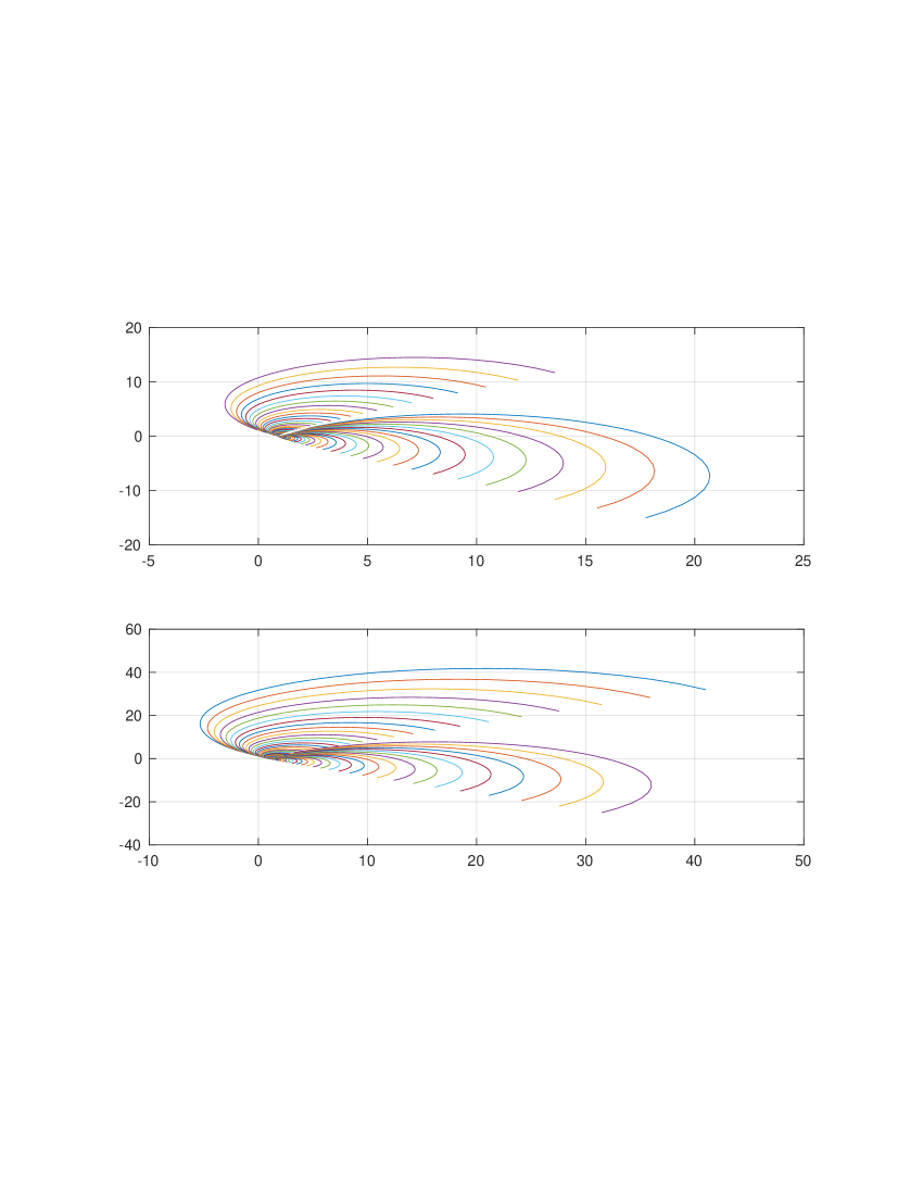
Figure 2. Plots of curves $\eta\mapsto(1-q)/(1-q\Phi(\eta))$, for $q$ in the SINH-$Z$- inversion and $\eta$ on the contours ${\mathcal{L}}^{\pm}$ (upper and lower panels) in the numerical example with $\nu=1.2$, and $T=15$.

In order that the deformation be justified, it is necessary that, in the process of the deformation, the fractions under the log-sign in (4.3) and (4.4) do not equal 0 for all $q$ and $\eta$ of interest; in order to avoid complications stemming from the analytic continuation to an appropriate Riemann surface, it is advisable to make sure that the fraction does not assume values in $(-\infty,0]$ in the process of the deformation. See Fig. 2 for an illustration.

Choice of $\omega^{\pm}.$ If $\gamma_{-}<0<\gamma_{+}$, then it is possible to choose $\omega^{-}\in(\gamma_{-},0)$ and $\omega^{+}\in(0,\gamma_{+})$. If $\gamma_{-}=0$, then both $\omega^{\pm}\in(0,\gamma_{+})$, and if $\gamma_{+}=0$, then both $\omega^{\pm}\in(\gamma_{-},0)$. When the double integral on the RHS of (3.8) is evaluated, we need to calculate the Wiener-Hopf factors at the points on two contours ${\mathcal{L}}^{\pm}:={\mathcal{L}}_{\omega^{\pm}_{1},b^{\pm},\omega^{\pm}}$. In order to increase the width of of the strip of analyticity of each of the integrands on the RHS’ of (4.3) and (4.4), one should take $\omega^{-}=\gamma_{-}+(\gamma_{+}-\gamma_{-})/3$, $\omega^{+}=\gamma_{+}-(\gamma_{+}-\gamma_{-})/3$.

In the case of Lévy processes of finite variation, with non-zero drift $\mu$, the characteristic function $\Phi_{\bar{\Delta}}$ is of the form $\Phi_{\bar{\Delta}}=e^{i\mu\bar{\Delta}\xi}\Phi^{0}_{\bar{\Delta}}$, where $\Phi^{0}_{\bar{\Delta}}$ obeys the bound (4.1) or (4.2) in a cone ${\mathcal{C}}_{\gamma_{-},\gamma_{+}}$, where $\gamma_{-}<0<\gamma_{+}$, with $\nu<1$. If $\mu>0$, $\Phi_{\bar{\Delta}}$ obeys the bound (4.1) or (4.2) in the cone ${\mathcal{C}}_{0,\gamma_{+}}$, and if $\mu<0$, then in the cone ${\mathcal{C}}_{\gamma_{-},0}$. If $\mu>0$, it is advantageous to calculate ${\phi^{-}_{q}}(\xi)$ using (4.4) with $\omega^{+}>0$, and then, if ${\phi^{+}_{q}}(\xi)$ is needed, use the Wiener-Hopf factorization identity. If $\mu<0$, it is advantageous to calculate ${\phi^{+}_{q}}(\xi)$ using (4.3) with $\omega^{-}<0$, and then, if ${\phi^{-}_{q}}(\xi)$ is needed, use (3.2).

4.3. Evaluation of the integrals on the RHS of (3.8)

If $x_{1}-a_{1}\geq 0$, it is advantageous to deform the line of integration upwards into a contour of the form ${\mathcal{L}}_{\omega^{+}_{1},b^{+},\omega^{+}}$, where $\omega^{+}>0$, and if $x_{1}-a_{1}\leq 0$, then into a a contour of the form ${\mathcal{L}}_{\omega^{-}_{1},b^{-},\omega^{-}}$, where $\omega^{-}<0$. If $x_{1}-a_{1}=0$, then any $\omega\in(\gamma_{-},\gamma_{+})$ is admissible, and $\omega=(\gamma_{-}+\gamma_{+})/2$ is (approximately) optimal. However, if $\Phi_{\bar{\Delta}}$ is of the form $\Phi_{\bar{\Delta}}=e^{i\mu\bar{\Delta}\xi}\Phi^{0}_{\bar{\Delta}}$, where $\Phi^{0}_{\bar{\Delta}}$ obeys the bound (4.1) or (4.2) in a cone ${\mathcal{C}}_{\gamma_{-},\gamma_{+}}$, where $\gamma_{-}<0<\gamma_{+}$, with $\nu<1$ and $\mu>0$, then the deformation with $\omega^{-}<0$ is impossible because, for $|q|=R<1$, $1-qe^{i\bar{\Delta}\mu\xi}\Phi^{0}_{\bar{\Delta}}(\xi)$ equals 0 for some $\xi$ in the process of deformation. In this case, as in [19], we use a less efficient family of conformal maps of the form

(4.5) $$\chi_{S;\omega,m,a}(y)=(y+i\omega)\ln^{m}(a^{2}+(y+i\omega)^{2}),$$

where $\omega\in{\mathbb{R}},a>|\omega|,$ and $m\geq 1$ is an integer. As $y\to\pm\infty$,

$$\chi_{S;\omega,m,a}(y)=(2\ln y)^{m}(y+i\omega(1+m/\ln|y|)+O(|y|^{-1}),$$

therefore, if we take $\omega<0$ and change the variable $\xi=\chi_{S;\omega,a,a}(y)$, then the exponent $e^{i\bar{\Delta}\mu\xi(y)}$ increases as $y\to\infty$ in a strip around ${\mathbb{R}}$ slower than the factor $\Phi_{\bar{\Delta}}^{0}(\xi(y))$ decays at infinity, and the product decays faster than prior to the change of variables. If $x_{1}-a_{1}>0$, we use $\omega>0$.

Consider the repeated integral. Since $x_{2}-a_{2}<0$, in the outer integral, we deform the line of integration so that the wings of the deformed contour point downwards. If the bound (4.1) (or (4.2)) holds in a cone ${\mathcal{C}}_{\gamma_{-},\gamma_{+}}$ where $\gamma_{-}<0$, we use the map $\chi_{\omega^{-}_{1},b^{-},\omega^{-}}$ with $\omega^{-}<0$. As in the case of 1D integral, it may be necessary to use the map $\chi_{S;\omega,m,a}$ with $\omega<0$. Since $a_{2}-a_{1}\geq 0$, in the inner integral, we deform the line of integration so that the wings of the deformed contour point upwards. If the bound (4.1) (or (4.2)) holds in a cone ${\mathcal{C}}_{\gamma_{-},\gamma_{+}}$ where $\gamma_{+}>0$, we use the map $\chi_{\omega^{+}_{1},b^{+},\omega^{+}}$. As in the case of 1D integral, it may be necessary to use the map $\chi_{S;\omega,m,a}$ with $\omega>0$. Note that a less efficient family of deformations must be used at most once in the 1D-integral, and at most once in the repeated integral, and, in all cases, the Wiener-Hopf factors can be calculated using the sinh-acceleration.

If (4.1) or (4.2) hold, then it is possible to find appropriate conformal deformations of the contours of integration in all formulas. In the case of Lévy processes of finite variation, with non-zero drift $\mu$, the characteristic function $\Phi_{\bar{\Delta}}$ is of the form $\Phi_{\bar{\Delta}}=e^{i\mu\bar{\Delta}\xi}\Phi^{0}_{\bar{\Delta}}$, where $\Phi^{0}_{\bar{\Delta}}$ obeys the bound (4.1) or (4.2) in a cone ${\mathcal{C}}_{\gamma_{-},\gamma_{+}}$, where $\gamma_{-}<0<\gamma_{+}$, with $\nu<1$, then the conformal deformation of the contour of integration in the $Z$-inversion formula is impossible, and only trapezoid rule can be applied.

5. Algorithm and numerical examples

We take $x_{1}=x_{2}=0$ and calculate the joint cpdf $F(T,a_{1},a_{2})=V(T,a_{1},a_{2};0,0)$ assuming that the cone of analyticity contains the real line: $\gamma_{-}<0<\gamma_{+}$. This allows us to use two contours in $\xi_{1}$ and $\eta$ planes for all purposes, one in the lower half-plane, the other in the upper half-plane. If either $\gamma_{-}=0$ or $\gamma_{+}=0$, then, firstly, in (3.8), one of the lines of integration can be deformed using the sinh-map, but the other line can deformed using a less efficient family of deformations only (see Sect. 4.3), and, secondly, for the calculation of the Wiener-Hopf factors, an additional “sinh-deformed” contour is needed. Hence, the total number of the contours is three, not two, as in the algorithm below.

1. Following the recommendation in Sect.2, choose either the parameters for the trapezoid rule $M_{0}$ and $M=2*M_{0}+1$ and construct the grid $\vec{q}=R*\exp((i*2*\pi/M)*(0:1:M_{0}))$ or choose the sinh-deformation and grid for the simplified trapezoid rule: $\vec{y}=\zeta_{\ell}*(0:1:M_{0})$, $\vec{q}=\sigma_{\ell}+i*b_{\ell}*\sinh(i*\omega_{\ell}+\vec{y})$. Calculate the derivative $\vec{der_{\ell}}=i*b_{\ell}*\cosh(i*\omega_{\ell}+\vec{y})$. Note that if double precision arithmetic is used, the choice of $R$, $\sigma_{\ell}$ and $b_{\ell}$ must depend on $T$ but can be independent of $x_{1},x_{2},a_{1},a_{2}$, at some loss in the efficiency of the algorithm. For large $n^{\prime}$s, this leads to a significant increase of the number of terms in the trapezoid rule. In the case of the sinh-acceleration, the effect is less pronounced but leads to worse results for very large $n$, as in the numerical examples for $T=15$ below.

2. Choose the sinh-deformations and grids for the simplified trapezoid rule on ${\mathcal{L}}^{\pm}$: $\vec{y^{\pm}}=\zeta^{\pm}*(-N^{\pm}:1:N^{\pm})$, $\vec{\xi^{\pm}}=i*\omega_{1}^{\pm}+b^{\pm}*\sinh(i*\omega^{\pm}+\vec{y^{\pm}})$. Calculate $\Phi^{\pm}=\Phi(\vec{\xi^{\pm}})$ and $\vec{der^{\pm}}=b^{\pm}*\cosh(i*\omega^{\pm}+\vec{y^{\pm}}).$

3. Calculate the arrays $D^{+}=[1/(\xi^{+}_{j}-\xi^{-}_{k})]$ and $D^{-}=[1/(\xi^{-}_{k}-\xi^{+}_{j})]$ (the sizes are $(2*N^{+}+1)\times(2*N^{-}+1)$ and $(2*N^{-}+1)\times(2*N^{+}+1)$, respectively).

4. The main block. For given $x_{1},x_{2},a_{1},a_{2}$, in the cycle in $q\in\vec{q}$, evaluate

   1. ${\phi^{+}_{q}}$ at points of the grid ${\mathcal{L}}^{+}$ and ${\phi^{-}_{q}}$ at points of the grid ${\mathcal{L}}^{-}$:

      $$\vec{\phi^{\pm}_{q}}=\exp\left[((\mp\zeta^{\pm}*i*\zeta^{\mp}/(2*\pi))*\vec{\xi^{\pm}}.*(\log((1-q)./(1-q\Phi^{\mp}))./\vec{\xi^{\mp}}.*\vec{der^{\mp}})*D^{\pm})\right];$$

   2. calculate $\phi^{\pm}_{q}$ at points of the grid ${\mathcal{L}}^{\mp}$: $\vec{\phi^{\pm}_{q,\mp}}=(1-q)./(1-q\Phi^{\mp})./\vec{\phi^{\mp}_{q}};$

   3. evaluate the 2D integral on the RHS of (3.8)

      $$Int2(q) = ((\zeta^{-}*\zeta^{+}/(2*\pi)^{2})*(\exp(-i*a_{2}*\vec{\xi^{-}}).*\vec{\phi^{+}_{q,-}}.*\vec{der^{-}})*D^{+})$$

      $$*\mathrm{conj}((\exp((i*(a_{2}-a_{1}))*\vec{\xi^{+}}).*\vec{\phi^{-}_{q,+}}/\vec{\xi^{+}}.*\vec{der^{+}})^{\prime}).$$

   4. if $x_{1}-a_{1}>0$, use arrays $\vec{\xi^{+}},\vec{der^{+}},\Phi^{+}$ to evaluate $Int1(q)$, the 1D integral on the RHS of (3.8); if $x_{1}\leq a_{1}$, use arrays $\vec{\xi^{-}},\vec{der^{-}},\Phi^{-}$ instead and add $1/(1-q)$;

   5. set $Int(q)=Int1(q)./(1-\vec{q})+Int2(q)$.

5. Set $Int(q_{1})=Int(q_{1})/2$.

6. If the sinh-acceleration is used for the inverse $Z$-transform, calculate

   $$V_{n}=(\zeta_{\ell}/\pi)*real(\mathrm{sum}(\vec{q}.^{-n-1}.*Int(\vec{q}).*\vec{der_{\ell}}));$$

   if the trapezoid rule is used, calculate

   $$V_{n}=(2/M)*real(\mathrm{sum}(\vec{q}.^{-n}.*Int(\vec{q})).$$

Numerical results are produced using Matlab R2017b on MacBook Pro, 2.8 GHz Intel Core i7, memory 16GB 2133 MHz. The CPU times reported below can be significantly improved because we use the same grids for the calculation of the Wiener-Hopf factors $\phi^{\pm}_{q}$ and evaluation of integrals on the RHS of (3.8). However, $\phi^{\pm}_{q}$ need to be evaluated only once and used for all points $(a_{1},a_{2})$. But if $x_{1}-a_{2}$ and $a_{2}-a_{1}$ are not very small in absolute value, then much shorter grids can be used. See, e.g., examples in [17, 41, 18, 20]. Therefore, if the arrays $(x_{1}-a_{2},a_{2}-a_{1})$ are large, then the CPU time can be decreased using shorter arrays for calculation of the integrals on the RHS of (3.8). Furthermore, the main blocks of the program admit the trivial parallelization.

In the two examples that we consider, the characteristic function is $\Phi(\xi)=e^{-\bar{\Delta}\psi(\xi)}$, where $\psi$ is the characteristic exponent $\psi(\xi)=c\Gamma(-\nu)(\lambda_{+}^{\nu}-(\lambda_{+}+i\xi)^{\nu}+(-\lambda_{-})^{\nu}-(-\lambda_{-}-i\xi)^{\nu})$ of a KoBoL process, where $\lambda_{+}=1,\lambda_{-}=-2$ and (I) $\nu=0.2$, hence, the process is close to Variance Gamma process; (II) $\nu=1.2$, hence, the process is close to the Normal Inverse Gaussian process (NIG). In both cases, $c>0$ is chosen so that the second instantaneous moment $m_{2}=\psi^{\prime\prime}(0)=0.1$. The time step is $\bar{\Delta}=1/252$ (daily monitoring). For $X_{0}={\bar{X}}_{0}=0$, we calculate the joint cpdf $F(T,a_{1},a_{2}):=V(T,a_{1},a_{2};0,0)$ for $T=15$ in Case (II) and for $T=0.25,1,5,15$ in Case (I). In both cases, $a_{1}$ is in the range $[-0.075,0.1]$ and $a_{2}$ in the range $[0.025,0.175]$; the total number of points $(a_{1},a_{2})$, $a_{1}\leq a_{2}$, is 44. We show the results for $T=0.25,5$ and $T=15$ because the errors, CPU times and sizes of arrays in the case $T=1$ can be approximated well by interpolation of the results for $T=0.25$ and $T=5$.

The numerical examples demonstrate the clear advantage of the sinh-acceleration applied to the inverse $Z$-transform vs the trapezoid rule; the advantage increases proportionally to the number of steps because the sinh-acceleration requires approximately the same number of terms of the simplified trapezoid rule whereas the number of terms in the trapezoid rule increases. Note, however, that if high precision arithmetic is used then the trapezoid rule with much smaller number of terms can be used.

We also show the errors of the approximation of the continuous time model with the model with daily monitoring. The probabilities in the continuous time model are calculated using the method in [21]. As expected, the approximation errors increase with the number of steps but remain fairly good even at $T=15$.

6. Conclusion

There exists a large body of literature devoted to calculation of expectations $V(f;T;x_{1},x_{2})$ of functions of spot value $x_{1}$ of $X$ and its running maximum or minimum $x_{2}$ and related optimal stopping problems, standard examples being barrier and American options, and lookback options with barrier and/or American features. See, e.g., [32, 10, 11, 12, 13, 40, 1, 2, 37, 36, 28, 15, 6, 4, 7, 39, 38, 16, 26, 25, 5, 24, 33, 29, 34, 35, 44, 27, 43, 20, 23] and the bibilographies therein. In many papers, in the infinite time horizon case, the Wiener-Hopf factorization technique in various forms is used, and the finite time horizon problems are reduced to the infinite time horizon case using the Laplace transform or its discrete version. The present paper belongs to this strand of the literature. We consider random walks, equivalently, in the context of option pricing, barrier and lookback options with discrete monitoring.

At the first step, as in [28], where barrier options with discrete monitoring in the Brownian motion model are priced, we use the $Z$-transform, which is the discrete time counterpart of the Laplace transform. The latter was used in the continuous time case in a number of publications starting with [10, 11]. The first contribution of the present paper is the new numerical method for the inverse $Z$-transform, which is more efficient than the trapezoid rule. In both continuous time and discrete time cases, the application of the Laplace and $Z$-transforms reduces the problem to pricing the corresponding options in the infinite time horizon. The second contribution of the present paper is a general formula for the expectation of a function of a random walk and its supremum process. The formula generalizes the formulas for the barrier options in the random walk and Lévy models derived in [10, 11, 13, 15, 6], and it is a counterpart of the general formula for the Lévy processes derived in [21]. Both formulas use the expected present value operators (EPV-operators) technique, which is the operator form of the Wiener-Hopf factorization. The last contribution of the paper is the set of efficient numerical realizations of the general formulas, which we explain in detail in the case of the calculation of the joint probability distribution of the random walk and its supremum. The numerical examples demonstrate that the method based on the sinh-acceleration for the inverse $Z$-transform can achieve the accuracy of the order of E-14 and better using Matlab and Mac with moderate characteristics, in a second or fraction of a second, and the precision of the order of E-10 in 20-30 msec., for options of maturity in the range $T=0.25-15Y$. In all cases, the sizes of the arrays are moderate. In particular, the number of points used for the $Z$-transform inversion is of the order of 2-5 dozens or even fewer. If the trapezoid rule is used, the size of arrays and CPU time increase with the maturity, and, for maturity $T=15$, approximately 3,000 terms are needed. When the trapezoid rule is applied, the CPU time is several times larger in all cases. We also compare the results in the case of continuous monitoring using the methods developed in [21] and demonstrate that in the case of daily monitoring, the relative differences are less than 1% even for $T=15$ for a process close to the Variance Gamma, and less than 5% for a process close to NIG.

Other methods for pricing barrier and lookback options with discrete monitoring cannot achieve the precision E-10 even at a much larger CPU cost. COS method [26, 25] introduces an additional source of errors, and the errors accumulate very fast. As numerical examples in [24] show, the errors of COS can be of the oder of 10% even for options of short maturity, and blow up for maturity $T=1Y$. BPROJ method [34, 35, 23] also introduces an error, which accumulates but not as fast as the error of COS. Furthermore, the error of the approximation of the transition density in BPROJ method is in the norm of the Sobolev space $H^{2}({\mathbb{R}})$, hence, very large for distributions close to the Variance Gamma - and, for small monitoring intervals, in the case of the Variance Gamma model, the $H^{2}$-norm is $+\infty$ (see [23] for the detailed analysis of COS, BROJ and filtering used in the literature to increase the speed of convergence - at the cost of additional errors). The Hilbert transform approach (see, e.g., [27, 29]) requires long grids, and the grids have to be extremely long for small time intervals and processes of finite variation. In addition, it is very difficult to accurately estimate the accumulation of errors. The method of [24], where the calculations are in the state space, allows one to derive sufficiently accurate error bounds and recommendations for the choice of the parameters of the numerical scheme. However, the grids must increase with time to maturity, and, in the result, for options of maturity more than a year, even the precision of the order of E-05 requires much more CPU time than the method of the present paper.

Appendix A Technicalities

A.1. Proof of Theorem 2.1

First, let $h(z)=z^{m}$ for some integer $m$. Then $T_{M}(h)=0$ if $M$ does not divide $m$, and $T_{M}(h)=1$ if $M$ divides $m$. This is a standard exercise about sums of roots of unity. Under conditions of the theorem, $h(z)$ has a Laurent series expansion $h(z)=\sum_{j\in{\mathbb{Z}}}b_{j}z^{j}$ which converges uniformly on the unit circle. Then $I(h)=b_{0}$ and $T_{n}(h)$ is the sum of $b_{j}$ for all $j$ that are divisible by $M$. Hence, $|T_{M}(h)-I(h)|$ is bounded by the sum of $|b_{j}|$, where $j$ ranges over all nonzero integers that are divisible by $M$. We have

$$b_{j} = \frac{1}{2\pi i}\int_{|z|=1}z^{-j-1}h(z)dz=\frac{1}{2\pi i}\int_{|z|=\rho}z^{-j-1}h(z)dz=\frac{1}{2\pi i}\int_{|z|=1/\rho}z^{-j-1}h(z)dz.$$

Hence,

$$\sum_{j>0}|b_{Mj}| \leq \sum_{j>0}\rho^{-Mj-1}\int_{|z|=\rho}|h(z)|\frac{dz}{2\pi i}=\frac{\rho^{-M}}{1-\rho^{-M}}\frac{1}{2\pi i}\int_{|z|=\rho}|h(z)|\frac{dz}{z},$$

and, similarly,

$$\sum_{j<0}|b_{Mj}|\leq\frac{\rho^{-M+1}}{1-\rho^{-M}}\frac{1}{2\pi i}\int_{|z|=1/\rho}|h(z)|\frac{dz}{z}.$$

Adding the two inequalities finishes the proof.

A.2. Proof of Proposition 3.2

(a) follows from the following three facts: $\Phi(0)=1$; $\Phi$ is continuous on $i[\lambda_{-},\lambda_{+}]$; and $|\Phi(\xi)|\leq\Phi(-\operatorname{\rm Im}\xi)$. (b) Take $\xi\in S_{(\mu_{-},\mu_{+})}$ and note that the integrands are analytic in $S_{[\mu_{-},\mu_{+}]}$, with the only simple pole at $\eta=\xi$ and decay as $|\eta|^{-2}$ as $(S_{[\mu_{-},\mu_{+}]}\ni)\eta\to\infty$ (the apparent singularity at $\eta=0$ is removable). By the residue theorem,

$$\ln\frac{1-q}{1-q\Phi(\eta)}=-\frac{1}{2\pi i}\int_{\operatorname{\rm Im}\xi=\omega_{-}}\frac{\xi\ln\frac{1-q}{1-q\Phi(\eta)}}{\eta(\xi-\eta)}d\eta+\frac{1}{2\pi i}\int_{\operatorname{\rm Im}\xi=\omega_{+}}\frac{\xi\ln\frac{1-q}{1-q\Phi(\eta)}}{\eta(\xi-\eta)}d\eta,$$

hence, (3.3) holds for $\phi^{\pm,^{\prime}}_{q}(\xi)$ given by the RHS’ of (3.4)-(3.5) and all $\xi\in S_{(\mu_{-},\mu_{+})}$. Since $\phi^{+,^{\prime}}_{q}$ and ${\phi^{+}_{q}}$ are analytic and uniformly bounded in the upper half-plane, and $\phi^{-,^{\prime}}_{q}$ and ${\phi^{-}_{q}}$ are analytic and uniformly bounded in the lower half-plane, (3.4)-(3.5) follow from the uniqueness of the Wiener-Hopf factorization.

(c) The integrals on the RHS’ of (3.4) and (3.5) do not change if we omit the factor $1-q$ under the log sign. Using $\xi/(\eta(\xi-\eta))=1/\eta+1/(\xi-\eta)$, we conclude that it suffices to prove that, for any $\epsilon>0$ and $A>0$, there exists $C_{A,\epsilon}>0$ such that for any $\xi\in S_{[-A,A]}$,

(A.1) $$\int_{\mathbb{R}}\frac{(1+|\eta|)^{-\delta}}{1+|\xi-\eta|}d\eta\leq C_{A,\epsilon}(1+|\xi|)^{-\delta+\epsilon}.$$

We consider the integrals over $I_{1}=\{\eta\ |\ |\eta|\leq(1+|\xi|)/2\}$, $I_{2}=\{\eta\ |\ |\eta|\geq 2(1+|\xi|)\}$ and $I_{3}=\{\eta\ |\ (1+|\xi|)/2\leq|\eta|\leq 2(1+|\xi|)\}$:

$$I_{1} \leq C(1+|\xi|)^{-1}\int_{0}^{(1+|\xi|)/2}(1+|\eta|)^{-\delta}d\eta=C_{1}(1+|\xi|)^{-\delta},$$

$$I_{2} \leq C(1+|\xi|)^{-1}\int_{2(1+|\xi|)}^{+\infty}|\eta|^{-1-\delta}d\eta=C_{1}(1+|\xi|)^{-\delta},$$

$$I_{3} \leq C(1+|\xi|)^{-\delta}\int_{(1+|\xi|)/2}^{2(1+|\xi|)}|\eta-\xi|^{-1}d\eta\leq C_{1}(1+|\xi|)^{-\delta}\ln(1+|\xi|),$$

where $C,C_{1}$ are independent of $\xi$.

Appendix B Figures and tables

Table 1. Joint cpdf $F(T,a_{1},a_{2}):={\mathbb{Q}}[X_{T}\leq a_{1},{\bar{X}}_{T}\leq a_{2}\ |\ X_{0}={\bar{X}}_{0}=0]$, and errors (rounded) and CPU time (in msec) of two numerical schemes. Discrete monitoring, the monitoring interval $\bar{\Delta}=1/252$, $T=0.25Y$, the number of time steps 63. KoBoL close to the Variance Gamma model, with an almost symmetric jump density, and no “drift”: $m_{2}=0.1$, $\nu=0.2,\lambda_{-}=-2,\lambda_{+}=1$. Errors are rounded, the CPU time is in milliseconds (average over 1000 runs).

$a_{2}/a_{1}$	-0.075	-0.05	-0.025	0	0.025
0.025	0.052873910286366	0.0650091858382787	0.0879288341672031	0.506532201212114	0.923468308358369
0.05	0.0534088530783456	0.0656338924464693	0.0886847807216264	0.507515090989102	0.925299214939269
0.075	0.0536456853005228	0.0659043877286091	0.0890004474115774	0.507896616129521	0.925793930891586
0.1	0.0537794257554031	0.0660548821001662	0.0891723010284717	0.508097111907463	0.926036138000489
0.175	0.0539628421387795	0.0662578446892915	0.0893989471374944	0.508353292242695	0.926330710592022

			$A$					B
$a_{2}/a_{1}$	-0.075	-0.05	-0.025	0	0.025	-0.075	-0.05	-0.025	0	0.025
0.025	4.03E-12	3.63E-12	2.61E-13	5.46E-12	1.88E-11	4.41E-12	4.10E-12	3.4179E-13	-9.25E-13	1.38E-11
0.05	4.17E-12	3.81E-12	4.583E-13	5.80E-12	2.38E-12	4.57E-12	4.32E-12	6.20E-13	-5.57E-13	-2.93E-12
0.075	4.09E-12	3.70E-12	3.26E-13	5.65E-12	3.14E-12	4.46E-12	4.18E-12	4.82E-13	-7.13E-13	-3.14E-12
0.1	3.89E-12	3.48E-12	5.87E-14	4.88E-12	1.78E-12	4.21E-12	3.91E-12	1.61E-13	-1.08E-12	-3.56E-12
0.175	4.03E-12	3.63E-12	2.31E-13	5.19E-12	1.10E-12	4.30E-12	4.0E-12	2.62E-13	-9.66E-13	-3.44E-12

Errors of the benchmark values: better than E-14, at some points, E-15. CPU time per 1 point: 980, per 44 points: 6,672.
A: Trapezoid rule, $M_{0}=99$, $N^{\pm}=124$. CPU time per 1 point: 30.9; per 44 points: 496.
B: SINH applied to the inverse $Z$-transform, with $M_{0}=16,N^{\pm}=124$. CPU time per 1 point 10.2, per 44 points: 73.5.

Table 2. Joint cpdf $F(T,a_{1},a_{2}):={\mathbb{Q}}[X_{T}\leq a_{1},{\bar{X}}_{T}\leq a_{2}\ |\ X_{0}={\bar{X}}_{0}=0]$, in the continuous time model, and errors (rounded) of approximation by the discrete time model, with the time step $\bar{\Delta}=1/252$. $T=0.25Y$. KoBoL close to the Variance Gamma model, with an almost symmetric jump density, and no “drift”: $m_{2}=0.1$, $\nu=0.2,\lambda_{-}=-2,\lambda_{+}=1$. Errors are rounded.

$a_{2}/a_{1}$	-0.075	-0.05	-0.025	0	0.025
0.025	0.0528532412024314	0.0649856679446126	0.0879014169039586	0.506498701211731	0.923417160799492
0.05	0.0533971065051704	0.0656207900757623	0.0886699612390502	0.507497961893706	0.925278586629322
0.075	0.0536378889312988	0.0658957955144885	0.0889908892581356	0.507885843291178	0.925781540582068
0.1	0.0537738608706033	0.0660488001673687	0.0891656084917806	0.508089681056682	0.926027783268804
0.175	0.05396033997440315	0.0662551510091756	0.0893960371866518	0.508350135593746	0.926327268956837

			$A$					B
$a_{2}/a_{1}$	-0.075	-0.05	-0.025	0	0.025	-0.075	-0.05	-0.025	0	0.025
2.07E-05	2.35E-05	2.742E-05	3.35E-05	5.11E-05	0.00039	0.00036	0.00031	6.61E-05	5.54E-05
0.05	1.17E-05	1.31E-05	1.48E-05	1.71E-05	2.06E-05	0.00022	0.00020	0.00017	3.38E-05	2.23E-05
0.075	7.80E-06	8.59E-06	9.56E-06	1.08E-05	1.24E-05	0.00015	0.00013	0.00011	2.12E-05	1.34E-05
0.1	5.56E-06	6.08E-06	6.693E-06	7.43E-06	8.36E-06	0.00010	9.21E-05	7.51E-05	1.46E-05	9.02E-06
0.175	2.50E-06	2.69E-06	2.91E-06	3.16E-06	3.44E-06	4.64E-05	4.07E-05	3.263E-05	6.21E-06	3.72E-06

Errors of the benchmark values in the continuous time model: better than E-14, at a number of points, better than E-15.
A: Errors of approximation of the continuous time model by the discrete time model, $\bar{\Delta}=1/252$.
B: Relative rrors of approximation of the continuous time model by the discrete time model, $\bar{\Delta}=1/252$.

Table 3. Joint cpdf $F(T,a_{1},a_{2}):={\mathbb{Q}}[X_{T}\leq a_{1},{\bar{X}}_{T}\leq a_{2}\ |\ X_{0}={\bar{X}}_{0}=0]$, and errors (rounded) and CPU time (in msec) of two numerical schemes. $T=5Y$. Discrete monitoring, the monitoring interval $\bar{\Delta}=1/252$, the number of time steps 1260. KoBoL close to the Variance Gamma model, with an almost symmetric jump density, and no “drift”: $m_{2}=0.1$, $\nu=0.2,\lambda_{-}=-2,\lambda_{+}=1$. Errors are rounded, the CPU time is in milliseconds (average over 1000 runs).

$a_{2}/a_{1}$	-0.075	-0.05	-0.025	0	0.025
0.025	0.322715785176063	0.341705312612668	0.362654563514927	0.385503065295135	0.402853073943893
0.05	0.36823129960626	0.390755656346763	0.415922513339139	0.444104383367338	0.469731888892867
0.075	0.396209256972821	0.420842816392821	0.448475971976962	0.479643744322071	0.509135503443898
0.1	0.415752842072438	0.44180038793114	0.471059131572705	0.504139671693882	0.535967402412399
0.175	0.450253847495689	0.478623894580305	0.510496476100609	0.546559667768138	0.581857694138651

			$A$					B
$a_{2}/a_{1}$	-0.075	-0.05	-0.025	0	0.025	-0.075	-0.05	-0.025	0	0.025
0.025	5.26E-11	5.40E-11	5.56E-11	5.70E-11	6.97E-11	1.72E-11	1.86E-11	2.04E-11	2.58E-11	4.38E-11
0.05	5.19E-11	5.27E-11	5.35E-11	5.38E-11	5.45E-11	9.46E-12	1.02E-11	1.11E-11	1.54E-11	2.10E-11
0.075	5.44E-11	5.50E-11	5.55E-11	5.55E-11	5.56E-11	6.30E-12	6.77E-12	7.35E-12	1.12E-11	1.62E-11
0.1	5.74E-11	5.78E-11	5.83E-11	5.80E-11	5.80E-11	4.80E-12	5.14E-12	5.58E-12	9.25E-12	1.40E-11
0.175	6.63E-11	6.66E-11	6.69E-11	6.66E-11	6.63E-11	2.52E-12	2.68E-12	2.91E-12	6.35E-12	1.08E-11

Errors of the benchmark values: better than E-14, at a number of points, better than E-15. CPU time per 1 point: 239, per 44 points: 2,019.
A: Trapezoid rule, $M_{0}=2844$, $N^{\pm}=144$. CPU time per 1 point: 812.4; per 44 points: 9,211.
B: SINH applied to the inverse $Z$-transform, with $M_{0}=19,N^{\pm}=137$. CPU time per 1 point 15.7, per 44 points: 111.8.

Table 4. Joint cpdf $F(T,a_{1},a_{2}):={\mathbb{Q}}[X_{T}\leq a_{1},{\bar{X}}_{T}\leq a_{2}\ |\ X_{0}={\bar{X}}_{0}=0]$, in the continuous time model, and errors (rounded) of approximation by the discrete time model, with the time step $\bar{\Delta}=1/252$. $T=5Y$. KoBoL close to the Variance Gamma model, with an almost symmetric jump density, and no “drift”: $m_{2}=0.1$, $\nu=0.2,\lambda_{-}=-2,\lambda_{+}=1$. Errors are rounded.

$a_{2}/a_{1}$	-0.075	-0.05	-0.025	0	0.025
0.025	0.322520199783594	0.341498771047289	0.362435915393477	0.385270783252495	0.402604045074505
0.05	0.368086705216705	0.390602983343428	0.415760934326279	0.443932843905084	0.469548901563007
0.075	0.396095198340728	0.420722495404712	0.448348786726241	0.479508955507981	0.50899215240333
0.1	0.415660121524435	0.441702681710183	0.470955990412814	0.50403055838718	0.535851652064689
0.175	0.45019937409531	0.47856666561315	0.510436280251142	0.546496264054607	0.581790803932632

			$A$					B
$a_{2}/a_{1}$	-0.075	-0.05	-0.025	0	0.025	-0.075	-0.05	-0.025	0	0.025
0.025	0.00020	0.00021	0.00022	0.00023	0.00025	0.00061	0.00060	0.00060	0.00060	0.00062
0.05	0.00015	0.00015	0.00016	0.00017	0.00018	0.00039	0.00039	0.00039	0.00039	0.00039
0.075	0.00011	0.00012	0.00013	0.00013	0.00014	0.00029	0.00029	0.00028	0.00028	0.00028
0.1	9.27E-05	9.77E-05	0.00010	0.00011	0.00012	0.00022	0.00022	0.00022	0.00022	0.00022
0.175	5.45E-05	5.72E-05	6.02E-05	6.34E-05	6.69E-05	0.00012	0.00012	0.00012	0.00012	0.00011

Errors of the benchmark values in the continuous time model: better than E-15, with a couple of exceptions.
A: Errors of approximation of the continuous time model by the discrete time model, $\bar{\Delta}=1/252$.

B: Relative errors of approximation of the continuous time model by the discrete time model, $\bar{\Delta}=1/252$.

Table 5. Joint cpdf $F(T,a_{1},a_{2}):={\mathbb{Q}}[X_{T}\leq a_{1},{\bar{X}}_{T}\leq a_{2}\ |\ X_{0}={\bar{X}}_{0}=0]$, and errors (rounded) and CPU time (in msec) of two numerical schemes. $T=15Y$. Discrete monitoring, the monitoring interval $\bar{\Delta}=1/252$, the number of time steps 3780. KoBoL close to the Variance Gamma model, with an almost symmetric jump density, and no “drift”: $m_{2}=0.1$, $\nu=0.2,\lambda_{-}=-2,\lambda_{+}=1$. Errors are rounded, the CPU time is in milliseconds (average over 1000 runs).

$a_{2}/a_{1}$	-0.075	-0.05	-0.025	0	0.025
0.025	0.273003522656352	0.275060714621777	0.276863384237128	0.278361438403706	0.279413583881186
0.05	0.325601636899453	0.328403204232286	0.330932690547093	0.333148630324321	0.334989330744591
0.075	0.364467787376584	0.367935193185576	0.371127846709011	0.37400815325999	0.376529331567823
0.1	0.396164068347951	0.400244732717707	0.404054649236343	0.407558402431724	0.410715394955968
0.175	0.467032161225892	0.472690792930844	0.47810575026395	0.483245070441871	0.488075079451549

			$A$					B
$a_{2}/a_{1}$	-0.075	-0.05	-0.025	0	0.025	-0.075	-0.05	-0.025	0	0.025
0.025	1.40E-10	1.41E-10	1.41E-10	1.41E-10	1.45E-10	4.50E-11	4.59E-11	4.67E-11	-9.51E-12	2.71E-11
0.05	1.56E-10	1.56E-10	1.56E-10	1.56E-10	1.56E-10	4.10E-11	4.18E-11	4.26E-11	-1.37E-11	-1.368E-11
0.075	1.70E-10	1.71E-10	1.719E-10	1.71E-10	1.71E-10	4.05E-11	4.13E-11	4.219E-11	-1.42E-11	-1.41E-11
0.1	1.84E-10	1.84E-10	1.84E-10	1.84E-10	1.84E-10	4.08E-11	4.16E-11	4.24E-11	-1.39E-11	-1.38E-11
0.175	2.18E-10	2.19E-10	2.19E-10	2.19E-10	2.18E-10	4.26E-11	4.34E-11	4.43E-11	-1.120E-11	-1.19E-11

Errors of the benchmark values: better than E-13, with a couple of exceptions. CPU time per 1 point: 548, per 44 points: 4,162.
A: Trapezoid rule, $M_{0}=8538$, $N^{\pm}=172$. CPU time per 1 point: 2,494; per 44 points: 25,613.
NB: the general recommendation for the choice of $M_{0}$ (the error tolerance E-10) is decreased by 50%.
B: SINH applied to the inverse $Z$-transform, with $M_{0}=65,N^{\pm}=144$. CPU time per 1 point 27.5, per 44 points: 319.9.

Table 6. Joint cpdf $F(T,a_{1},a_{2}):={\mathbb{Q}}[X_{T}\leq a_{1},{\bar{X}}_{T}\leq a_{2}\ |\ X_{0}={\bar{X}}_{0}=0]$, in the continuous time model, and errors (rounded) of approximation by the discrete time model, with the time step $\bar{\Delta}=1/252$. $T=15Y$. KoBoL close to the Variance Gamma model, with an almost symmetric jump density, and no “drift”: $m_{2}=0.1$, $\nu=0.2,\lambda_{-}=-2,\lambda_{+}=1$. Errors are rounded.

$a_{2}/a_{1}$	-0.075	-0.05	-0.025	0	0.025
0.025	0.272804820564476	0.274859824870105	0.276660421125814	0.278156527723931	0.279206809800465
0.05	0.325434820584041	0.328234181455624	0.33076152710125	0.332975399214234	0.33481410584792
0.075	0.364320938273655	0.36778614523566	0.370976636656939	0.373854823172472	0.376373926428562
0.1	0.39603236911559	0.400110870613695	0.403918641220246	0.407420269437458	0.410575160782172
0.175	0.466932999301196	0.472589684334096	0.47800268074549	0.483140027197031	0.487968050938338

			$A$					B
$a_{2}/a_{1}$	-0.075	-0.05	-0.025	0	0.025	-0.075	-0.05	-0.025	0	0.025
0.025	0.00020	0.00020	0.00020	0.00021	0.00021	0.00073	0.00073	0.00073	0.00074	0.00074
0.05	0.00017	0.00017	0.00017	0.00017	0.00017	0.00051	0.00052	0.00052	0.00052	0.00052
0.075	0.00015	0.00015	0.00015	0.00015	0.00016	0.00040	0.00040	0.00041	0.00041	0.00041
0.1	0.00013	0.00013	0.00014	0.00014	0.00014	0.00033	0.00033	0.00034	0.00034	0.00034
0.175	9.92E-05	0.00010	0.00010	0.00010	0.00011	0.00021	0.00021	0.00022	0.00022	0.00022

Errors of the benchmark values in the continuous time model: better than E-13, with a couple of exceptions.
A: Errors of approximation of the continuous time model by the discrete time model, $\bar{\Delta}=1/252$.

B: Relative errors of approximation of the continuous time model by the discrete time model, $\bar{\Delta}=1/252$.

Table 7. Joint cpdf $F(T,a_{1},a_{2}):={\mathbb{Q}}[X_{T}\leq a_{1},{\bar{X}}_{T}\leq a_{2}\ |\ X_{0}={\bar{X}}_{0}=0]$, and errors (rounded) and CPU time (in msec) of two numerical schemes. $T=15Y$. Discrete monitoring, the monitoring interval $\bar{\Delta}=1/252$, the number of time steps 3780. KoBoL close to NIG, with an almost symmetric jump density, and no “drift”: $m_{2}=0.1$, $\nu=1.2,\lambda_{-}=-2,\lambda_{+}=1$. Errors are rounded, the CPU time is in milliseconds (average over 1000 runs).

$a_{2}/a_{1}$	-0.075	-0.05	-0.025	0	0.025
0.025	0.08750889022257	0.0876433202115771	0.0877488959582886	0.0878234438630917	0.0878604203790796
0.05	0.133430426595114	0.133678790617469	0.133884632610215	0.134046292415956	0.13416044157208
0.075	0.172212077596399	0.172587459419214	0.172909022548126	0.173175531405955	0.173384836452991
0.1	0.206872444504732	0.207388307897551	0.207840301897249	0.208227492747064	0.208548393051015
0.175	0.295589651996839	0.296599359388506	0.297519605986825	0.298349844042413	0.299089406243993

			$A$					B
$a_{2}/a_{1}$	-0.075	-0.05	-0.025	0	0.025	-0.075	-0.05	-0.025	0	0.025
0.025	-3.95E-10	-4.66E-10	-5.44E-10	1.06E-09	4.637E-10	4.68E-11	4.69E-11	4.16E-11	-6.00E-11	-5.90E-11
0.05	-5.48E-10	-6.63E-10	-7.95E-10	7.44E-10	7.73E-10	5.70E-11	5.94E-11	5.57E-11	-4.62E-11	-8.14E-11
0.075	-6.54E-10	-8.08E-10	-9.90E-10	4.86E-10	4.33E-10	6.063E-11	6.49E-11	6.33E-11	-3.66E-11	-7.06E-11
0.1	1.84E-10	1.84E-10	1.84E-10	1.84E-10	1.84E-10	6.09E-11	6.62E-11	6.61E-11	-3.21E-11	-6.42E-11
0.175	-6.65E-10	-8.321E-10	-1.03E-09	4.21E-10	3.37E-10	5.80E-11	6.34E-11	6.38E-11	-3.32E-11	-6.34E-11

Errors of the benchmark values: better than $5\cdot 10^{-13}$. CPU time per 1 point: 1,848, per 44 points: 20,263.
A: Trapezoid rule, $M_{0}=8538$, $N^{\pm}=172$. CPU time per 1 point: 3,046; per 44 points: 35,481.
NB: the general recommendation for the choice of $M_{0}$ (the error tolerance E-10) is decreased by 47%.
B: SINH applied to the inverse $Z$-transform, with $M_{0}=28,N^{\pm}=183$. CPU time per 1 point 27.5, per 44 points: 219.9.

Table 8. Joint cpdf $F(T,a_{1},a_{2}):={\mathbb{Q}}[X_{T}\leq a_{1},{\bar{X}}_{T}\leq a_{2}\ |\ X_{0}={\bar{X}}_{0}=0]$, in the continuous time model, and errors (rounded) of approximation by the discrete time model, with the time step $\bar{\Delta}=1/252$. $T=15Y$. KoBoL close to NIG, with an almost symmetric jump density, and no “drift”: $m_{2}=0.1$, $\nu=1.2,\lambda_{-}=-2,\lambda_{+}=1$. Errors are rounded.

$a_{2}/a_{1}$	-0.075	-0.05	-0.025	0	0.025
0.025	0.083599231183863	0.083725522194071	0.0838241629685378	0.0838929695457668	0.0839249287233805
0.05	0.130217710987261	0.130456839782095	0.130654399607263	0.130808705570046	0.13091634106018
0.075	0.169363038877019	0.169728032397852	0.170040043384744	0.170297815998657	0.170499151715123
0.1	0.204270598983103	0.204774983963964	0.205216260776888	0.205593481299844	0.205905127535884
0.175	0.293472724302235	0.294468206269081	0.295374834640356	0.296192060853885	0.296919211526691

			$A$					B
$a_{2}/a_{1}$	-0.075	-0.05	-0.025	0	0.025	-0.075	-0.05	-0.025	0	0.025
0.025	0.0039	0.0039	0.0039	0.0039	0.0039	0.047	0.047	0.047	0.047	0.047
0.05	0.0032	0.0032	0.0032	0.0032	0.0032	0.025	0.025	0.025	0.025	0.025
0.075	0.0028	0.0029	0.0029	0.0029	0.0029	0.017	0.017	0.017	0.017	0.017
0.1	0.013	0.013	0.013	0.013	0.013	0.00033	0.00033	0.00034	0.00034	0.00034
0.175	0.0021	0.0021	0.0021	0.0022	0.0022	0.0072	0.00721	0.0073	0.0073	0.0073

Errors of the benchmark values in the continuous time model: better than E-13, with a couple of exceptions.
A: Errors of approximation of the continuous time model by the discrete time model, $\bar{\Delta}=1/252$.

B: Relative errors of approximation of the continuous time model by the discrete time model, $\bar{\Delta}=1/252$.

References

- [1] S. Asmussen, F. Avram, and M.R. Pistorius. Russian and American put options under exponential phase-type Lévy models. Stochastic Processes and their Applications, 109(1):79–111, 2004.
- [2] F. Avram, A. Kyprianou, and M.R. Pistorius. Exit problems for spectrally negative Lévy processes and applications to (Canadized) Russian options. Annals of Applied Probability, 14(2):215–238, 2004.
- [3] A.A. Borovkov. Stochastic processes in queueing theory. Springer-Verlag, Berlin, 1976.
- [4] M. Boyarchenko and S. Boyarchenko. Double barrier options in regime-switching hyper-exponential jump-diffusion models. International Journal of Theoretical and Applied Finance, 14(7):1005–1044, 2011.
- [5] M. Boyarchenko, M. de Innocentis, and S. Levendorskiĭ. Prices of barrier and first-touch digital options in Lévy-driven models, near barrier. International Journal of Theoretical and Applied Finance, 14(7):1045–1090, 2011. Available at SSRN: http://papers.ssrn.com/abstract=1514025.
- [6] M. Boyarchenko and S. Levendorskiĭ. Prices and sensitivities of barrier and first-touch digital options in Lévy-driven models. International Journal of Theoretical and Applied Finance, 12(8):1125–1170, December 2009.
- [7] M. Boyarchenko and S. Levendorskiĭ. Valuation of continuously monitored double barrier options and related securities. Mathematical Finance, 22(3):419–444, July 2012.
- [8] S. Boyarchenko and S. Levendorskiĭ. Generalizations of the Black-Scholes equation for truncated Lévy processes. Working Paper, University of Pennsylvania, April 1999.
- [9] S. Boyarchenko and S. Levendorskiĭ. Option pricing for truncated Lévy processes. International Journal of Theoretical and Applied Finance, 3(3):549–552, July 2000.
- [10] S. Boyarchenko and S. Levendorskiĭ. Barrier options and touch-and-out options under regular Lévy processes of exponential type. Annals of Applied Probability, 12(4):1261–1298, 2002.
- [11] S. Boyarchenko and S. Levendorskiĭ. Non-Gaussian Merton-Black-Scholes Theory, volume 9 of Adv. Ser. Stat. Sci. Appl. Probab. World Scientific Publishing Co., River Edge, NJ, 2002.
- [12] S. Boyarchenko and S. Levendorskiĭ. Perpetual American options under Lévy processes. SIAM Journal on Control and Optimization, 40(6):1663–1696, 2002.
- [13] S. Boyarchenko and S. Levendorskiĭ. Pricing of perpetual Bermudan options. Quantitative Finance, 2:422–432, 2002.
- [14] S. Boyarchenko and S. Levendorskiĭ. American options: the EPV pricing model. Annals of Finance, 1:267–292, 2005.
- [15] S. Boyarchenko and S. Levendorskiĭ. Irreversible Decisions Under Uncertainty (Optimal Stopping Made Easy). Springer, Berlin, 2007.
- [16] S. Boyarchenko and S. Levendorskiĭ. Efficient Laplace inversion, Wiener-Hopf factorization and pricing lookbacks. International Journal of Theoretical and Applied Finance, 16(3):1350011 (40 pages), 2013. Available at SSRN: http://ssrn.com/abstract=1979227.
- [17] S. Boyarchenko and S. Levendorskiĭ. Efficient variations of Fourier transform in applications to option pricing. Journal of Computational Finance, 18(2):57–90, 2014. Available at http://ssrn.com/abstract=1673034.
- [18] S. Boyarchenko and S. Levendorskiĭ. Sinh-acceleration: Efficient evaluation of probability distributions, option pricing, and Monte-Carlo simulations. International Journal of Theoretical and Applied Finance, 22(3), 2019. DOI: 10.1142/S0219024919500110. Available at SSRN: https://ssrn.com/abstract=3129881 or http://dx.doi.org/10.2139/ssrn.3129881.
- [19] S. Boyarchenko and S. Levendorskiĭ. Conformal accelerations method and efficient evaluation of stable distributions. Acta Applicandae Mathematicae, 169:711–765, 2020. Available at SSRN: https://ssrn.com/abstract=3206696 or http://dx.doi.org/10.2139/ssrn.3206696.
- [20] S. Boyarchenko and S. Levendorskiĭ. Static and semi-static hedging as contrarian or conformist bets. Mathematical Finance, 3(30):921–960, 2020. Available at SSRN: https://ssrn.com/abstract=3329694 or http://arxiv.org/abs/1902.02854.
- [21] S. Boyarchenko and S. Levendorskiĭ. Efficient evaluation of expectations of functions of a lévy process and its extremum. Working paper, June 2022. Available at SSRN: https://ssrn.com/abstract=4140462 or http://arxiv.org/abs/4362928.
- [22] S. Boyarchenko and S. Levendorskiĭ. Lévy models amenable to efficient calculations. Working paper, June 2022. Available at SSRN: https://ssrn.com/abstract=4116959 or http://arxiv.org/abs/4339862.
- [23] S. Boyarchenko, S. Levendorskiĭ, J.L. Kirkby, and Z. Cui. SINH-acceleration for B-spline projection with option pricing applications. International Journal of Theoretical and Applied Finance, -(-), 2022. Available at SSRN: https://ssrn.com/abstract=3921840 or arXiv:2109.08738.
- [24] M. de Innocentis and S. Levendorskiĭ. Pricing discrete barrier options and credit default swaps under Lévy processes. Quantitative Finance, 14(8):1337–1365, 2014. Available at: DOI:10.1080/14697688.2013.826814.
- [25] F. Fang, H. Jönsson, C.W. Oosterlee, and W. Schoutens. Fast valuation and calibration of credit default swaps under Lévy dynamics. Journal of Computational Finance, 14(2):57–86, Winter 2010.
- [26] F. Fang and C.W. Oosterlee. Pricing early-exercise and discrete barrier options by Fourier-cosine series expansions. Numerische Mathematik, 114(1):27–62, 2009.
- [27] L. Feng and V. Linetsky. Computing exponential moments of the discrete maximum of a Lévy process and lookback options. Finance and Stochastics, 13(4):501–529, 2009.
- [28] G. Fusai, I.D. Abrahams, and C. Sguarra. An exact analytical solution for discrete barrier options. Finance and Stochastics, 10(1):1–26, 2006.
- [29] G. Fusai, G. Germano, and D. Marazzina. Spitzer identity, Wiener-Hopf factorization and pricing of discretely monitored exotic options. European Journal of Operational Research, 251(1):124–134, 2016. DOI:10.1016/j.ejor.2015.11.027.
- [30] P. Greenwood and J. Pitman. Fluctuation identities for Lévy processes and splitting at the maximum. Advances in Applied Probability, 12(4):893–902, 1980.
- [31] P. Greenwood and J. Pitman. Fluctuation identities for random walk by path decomposition at the maximum. Advances in Applied Probability, 12(2):291–293, 1980.
- [32] X. Guo and L.A. Shepp. Some optimal stopping problems with nontrivial boundaries for pricing exotic options. J.Appl. Probability, 38(3):647–658, 2001.
- [33] G.G. Haislip and V.K. Kaishev. Lookback option pricing using the Fourier transform B-spline method. Quantitative Finance, 14(5):789–803, 2014.
- [34] J.L. Kirkby. American and Exotic Option Pricing with Jump Diffusions and other Lévy processes. Journ. Comp. Fin., 22(3):13–47, 2018.
- [35] J.L. Kirkby, D. Nguen, and Z. Cui. A unified approach to bermudan and barrier options under stochastic volatility models with jumps. Journal of Economic Dynamics and Control, 80(1):75–100, 2017.
- [36] S.G. Kou. A jump-diffusion model for option pricing. Management Science, 48(8):1086–1101, August 2002.
- [37] S.G. Kou and H. Wang. First passage times of a jump diffusion process. Adv. Appl. Prob., 35(2):504–531, 2003.
- [38] O. Kudryavtsev and S.Z. Levendorskiĭ. Efficient pricing options with barrier and lookback features under Lévy processes. Working paper, June 2011. Available at SSRN: 1857943.
- [39] A. Kuznetsov. Wiener-Hopf factorization and distribution of extrema for a family of Lévy processes. Ann.Appl.Prob., 20(5):1801–1830, 2010.
- [40] S. Levendorskiĭ. Pricing of the American put under Lévy processes. International Journal of Theoretical and Applied Finance, 7(3):303–335, May 2004.
- [41] S. Levendorskiĭ. Efficient pricing and reliable calibration in the Heston model. International Journal of Theoretical and Applied Finance, 15(7), 2012. 125050 (44 pages).
- [42] S. Levendorskiĭ. Method of paired contours and pricing barrier options and CDS of long maturities. International Journal of Theoretical and Applied Finance, 17(5):1–58, 2014. 1450033 (58 pages).
- [43] L. Li and V. Linetsky. Discretely monitored first passage problems and barrier options: an eigenfunction expansion approach. Finance and Stochastics, 19(3):941–977, 2015.
- [44] V. Linetsky. Spectral methods in derivatives pricing. In J.R. Birge and V. Linetsky, editors, Handbooks in OR & MS, Vol. 15, pages 223–300. Elsevier, New York, 2008.
- [45] L.C.G. Rogers and D. Williams. Diffusions, Markov Processes, and Martingales. Volume 1. Foundations. John Wiley & Sons, Ltd., Chichester, 2nd edition, 1994.
- [46] K. Sato. Lévy processes and infinitely divisible distributions, volume 68 of Cambridge Stud. Adv. Math. Cambridge University Press, Cambridge, 1999.
- [47] F. Stenger. Numerical Methods based on Sinc and Analytic functions. Springer-Verlag, New York, 1993.