Unveiling The Origin of Peculiar Diffuse Radio Emission in Abell 1351

Abstract

Abell 1351 is a massive merging cluster that hosts a giant radio halo and a bright radio edge blended in the halo. In this paper, we present the first ever spectral analysis of this cluster using GMRT 610 MHz and VLA 1.4 GHz archival data and discuss the radio edge property. Using Chandra data, we report the first tentative detection of shock front at the location of the edge in A1351 with discontinuities in both X-ray surface brightness and temperature. Our analysis strengthens the previous claim of the detected ”edge” being a high luminosity radio relic. The radio relic has an integrated spectral index $\alpha=-1.63\pm 0.33$ and radio power $P_{1.4\mathrm{\ GHz}}=4.46\pm 0.61\times 10^{24}$ W $Hz^{-1}$ with a largest Linear Size (LLS) of 570 kpc. The radio spectral index map shows steepening in the shock downstream region. Our analysis favours the scenario where the Diffusive Shock Acceleration (DSA) of particles is responsible for the origin of the radio relic in the presence of strong magnetic field. We have also estimated the magnetic field at the relic location assuming equipartition condition.

1 Introduction

Galaxy clusters play a significant role in the study of the large-scale particle acceleration process. These clusters are a concoction of dark matter, galaxies, and hot gas. The hot gas in the Intra-Cluster Medium (ICM) takes upto 15 - 17% of cluster total mass (van Weeren et al. 2019), and it emits in the X-ray band through the thermal bremsstrahlung process. Thus X-ray observations provide crucial information about cluster mass and dynamical state (Sarazin, 2002). The gravitational potential energy released during cluster mergers heats the ICM and is channeled through shocks and turbulence in the ICM. These shocks and turbulence accelerate relativistic particles and amplify magnetic fields. As a result, we get large-scale non-thermal synchrotron emissions from clusters in radio wavelength. These diffuse radio emissions come from highly relativistic particles spiraling around cluster magnetic fields and generally show a steep integrated spectral index ($\alpha<-1$ , where $S_{\nu}\propto\nu^{-\alpha}$) (van Weeren et al., 2019). The emissions are categorised as halo, minihalo, relic, and phoenix (Feretti et al., 2012; van Weeren et al., 2019). Halos and minihalos are centrally located diffuse structures. Halos are formed in the Megaparsec scale (size $\sim$ 0.5 - 2 Mpc) in massive merging clusters as a result of turbulent re-acceleration of relativistic electrons in the ICM (Brunetti & Jones, 2014). In comparison, minihalos (size $\sim$ 100 - 500 kpc) are seen in relaxed and cool core clusters mainly and are formed due to minor merger or gas sloshing or due to AGN feedback (ZuHone et al., 2013; Raja et al., 2020; Richard-Laferrière et al., 2020). The cluster radio relics are found mainly at the cluster outskirts or peripheral region (Enßlin, T. A. & Gopal-Krishna, 2001), generally have an elongated shape, and are polarised at high frequency. The relics can have the largest linear size (LLS) extending upto 3 Mpc (Hoang et al., 2021). The relics often coincide with cluster merger shocks. This spatial coincidence backs up the idea that relics are shock-generated. The formation of relics, for some clusters, is supported by the theory of Diffusive Shock Acceleration (DSA) of particles where the particles are accelerated to relativistic speed at the shock front from the thermal pool of Intra-Cluster Medium (ICM) (Drury, 1984; Ensslin et al., 1998; Hoeft & Brüggen, 2007; Kang & Ryu, 2013). However, the DSA mechanism is questioned by the particle acceleration efficiency of weak shocks that are generally observed in clusters (Hoeft & Brüggen, 2007; Botteon et al., 2016a; Gennaro et al., 2018). The reported relic luminosities and Mach numbers inferred from radio and X-ray observations point to another possibility where the shock re-accelerates the slightly relativistic old fossil plasma existing in the ICM. This theory is consistent with weaker shocks for generating luminous radio relics (Botteon et al., 2016a; van Weeren et al., 2017; Stuardi et al., 2019; Rajpurohit et al., 2020a). In another scenario, the shock adiabatically compresses an old AGN bubble and re-energizes fossil plasma. This phenomena is responsible for the generation of radio phoenixes at smaller cluster-centric distance (Enßlin, T. A. & Gopal-Krishna 2001; Slee et al. 2001; Enßlin & Brüggen 2002; Kempner et al. 2003; Ferrari et al. 2008). These radio phoenixes have a rather roundish and filamentary morphology, mostly show ultra-steep spectra with $\alpha<-2$ and also hint of spectral curvature at high-frequency (Slee et al., 2001; Kale et al., 2018; Mandal et al., 2019). Despite the available multi-wavelength study, exact particle acceleration mechanisms in the formation of diffuse radio emission are still to be understood properly. Also, we need to increase observational evidence to establish the correlations between cluster properties and diffuse emission.
Abell 1351 (A1351) is a massive ($M=1.4-4.2\times 10^{15}\ \mathrm{M}_{\odot}$) merging cluster at a redshift 0.325 (Barrena et al., 2014, hereafter B14). It has a mass distribution extended along the north-northeast (N-NE) and south-southwest (S-SW) direction (Bohringer et al. 2000; Dahle et al. 2002, B14). The presence of diffuse radio emission in A1351 was first detected by Owen et al. 1999. Using Karl G. Jansky Very Large Array (VLA) 1.4 GHz data Giacintucci et al. 2009; Giovannini et al. 2009 classified this Mpc scale diffuse emission in the cluster as giant radio halo. The halo is also detected by Botteon et al. 2022 using LOFAR Two-meter Sky Survey Data Release 2 (LoTSS-DR2). As reported previously, the cluster has an X-ray luminosity of $L_{x}(0.1-2.4\ \mathrm{keV})=8.31\times 10^{44}\ \mathrm{h}_{50}^{-2}\ \mathrm{ergs}^{-1}$ (Bohringer et al., 2000) and a radio luminosity $P_{1.4\mathrm{\ GHz}}=1.2-1.3\times 10^{25}$ h${}^{-2}_{70}$ W Hz^-1 (Giacintucci et al., 2009; Giovannini et al., 2009). The diffuse emission shows a bright edge at radio wavelength, which was classified as a ”ridge” by Giacintucci et al. 2009 (hereafter G09). Previously bright radio edge blended with the halo emission has been noticed in a few clusters (eg. Brown & Rudnick 2011; Macario et al. 2011; Shimwell et al. 2014; Wang et al. 2018). Both G09 and B14 suggested the complex, diffuse structure of A1351 can be a halo relic combination. Here we present the first ever spectral index map of the diffuse emission in A1351 using Giant Metrewave Radio Telescope (GMRT) 610 MHz and VLA 1.4 GHz data. We also analyzed Chandra X-ray data to look for a possible hint of shock front at the location of the radio-bright edge.

Table 1: A1351 Cluster properties

Parameter	Value
RAJ2000	11h 42m 30.8s
DECJ2000	$+58d\ 32\arcmin\ 20\arcsec$
Mass (Msys)	$1.4-4.2\times 10^{15}\ \mathrm{M}_{\odot}$
Redshift ($z$)	0.325
$L_{x}(0.1-2.4\ \mathrm{keV})$	8.31$\times 10^{44}\ \mathrm{h_{50}^{-2}\ erg\ s^{-1}}$
kT	$8.69^{+1.01}_{-0.54}$ keV
$\sigma_{v}$	$1524^{+96}_{-74}\ \mathrm{km\ s^{-1}}$

The outline of the paper is as follows. We present the radio observations and data reduction procedure from GMRT and VLA in section 2. In Section 3 we present the results from radio observation. We discuss about the X-ray observation and results in section 4 and  5 respectively. We discuss about the diffuse emission property, particle acceleration mechanism and cluster magnetic field in Section 6, followed by a summary in Section 7. We have assumed a $\Lambda$CDM cosmology with $\Omega_{m}$ = 0.3, $\Omega_{\lambda}$ = 0.7 and $H_{0}$ =70 km s^-1 Mpc^-1 throughout this paper. At the redshift of the Abell 1351 ($z=0.325$), 1″corresponds to 4.704 kpc.

2 Radio Observation

In this section, we discuss the observation and data reduction procedure of A1351 with GMRT 610 MHz and VLA 1.4 GHz.

Table 2: The archival observation summary for GMRT and VLA and the RMS reached using uniform weighting are listed below

Telescope	Observation date	Frequency	Bandwidth	Time on Source	Beam	P.A.	RMS
Configuration		( MHz)	( MHz)	(min)			($\mu$ Jy/beam)
GMRT	Feb 2010	610	30	865	$3.87\arcsec\times 3.40\arcsec$	$+31.50$°	105
VLA A	April 1994	1400	43.75	30	$1.38\arcsec\times 1.04\arcsec$	$-3.79$°	47
VLA C	April 2000	1400	43.75	125	$12.79\arcsec\times 9.76\arcsec$	$+28.43$°	42
VLA D	March 1995	1400	43.75	15	$51.32\arcsec\times 33.55\arcsec$	$+49.98$°	244

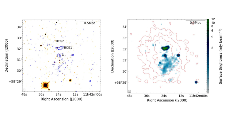
Figure 1: Left: GMRT 610 MHz high resolution image contours (blue) with restoring beam $3.87\arcsec\times 3.40\arcsec$, P.A $31.50\degree$ overlapped with SDSS-DR12 Optical image. The contours levels increases with a factor of 3 starting from 3$\sigma_{\mathrm{rms}}$ where $\sigma_{\mathrm{rms}}=105\ \mu$Jy/beam. Right: GMRT 610 MHz full resolution color image with restoring beam $5.17\arcsec\times 4.67\arcsec,$ P.A 46.06$\degree$ overlaid with red X-ray contours. The X-ray contours levels increases with a factor of 2.

2.1 GMRT 610 MHz

The cluster was observed with GMRT during Feb 2010 (project code 17_019 ) in dual-frequency (610 / 235 MHz) mode where the 610 MHz and 235 MHz visibilities are observed on RR and LL polarisation, respectively, with 865 min on-source time. For the GMRT Hardware Backened correlator, the bandwidth was split into upper and lower sidebands (USB and LSB), each having 16 MHz. For the two sidebands, .lta and .ltb files were generated for both frequencies. The observational summary of the cluster is presented in Table 2.

Source Peeling and Atmospheric Modelling (SPAM); (Intema, H. T. et al. 2009, 2017), a python-based data reduction recipe, was used for the GMRT data reduction. This semi-automated pipeline uses Astronomical Image Processing System (AIPS) tasks for data reduction. At first, The raw data in FITS format was used for pre-calibration. In the pre-calibration part, the data from the best available scans of the primary calibrator (here 3C286) was used for calibration. Scaife & Heald 2012 model was used to set the flux density. For 610 MHz, data for two sidebands were pre-calibrated separately and then joined. For 235 MHz, only part of the bandwidth (USB) was available for pre-calibration. The pre-calibrated visibility data set of UVFITS format was used for further process. After RFI mitigation and bad data editing, several rounds of direction-independent self-calibration were performed. Finally, direction-dependent calibration was done for 610 MHz data to correct ionospheric phase errors by peeling the bright sources within the field of view. Due to the poor data quality, the direction-dependent approach could not be applied for 235 MHz, and due to the poor image sensitivity, it was not further used in our analysis. The final calibrated dataset, obtained in FITS format, was converted to Common Astronomy Software Application (CASA) measurement set (.ms) format using the CASA task importgmrt. Further imaging was done in CASA.

2.1.1 Imaging Diffuse Emission at 610 MHz

In the full resolution ($5.17\arcsec\times 4.67\arcsec$, P.A. 46.06$\degree$) image of the cluster (Fig. 1 right panel) made using Briggs (Briggs, 1995) robust 0, the presence of diffuse emission is visible along with the discrete radio galaxies. This bright extended emission corresponds to the halo edge or the ridge emission of A1351. The edge has a rough extension of 570 kpc at 610 MHz. To bring out the diffuse emission properly, at first, we made a high-resolution image using Briggs (Briggs, 1995) robust parameter -1 and selecting uv-range greater than 1.7 k$\lambda$ (which roughly corresponds to 570 kpc at the redshift of 0.325) to ignore any contribution from the extended emission. We masked the individual radio galaxies from this image. We obtained the model visibility of these masked galaxies using CASA task tclean on the full dataset. These model visibilities were subtracted from the data using task uvsub in CASA. The final image for the diffuse emission was then made using Briggs robust 0, selecting a uv-range below 20 k$\lambda$ and using 5 k$\lambda$ uv-taper with a restoring beam $22.46\arcsec\times 19.88\arcsec$, P.A. $14.03\degree$ (Figure 2 color map). This choice of tapering and uv-range helped in achieving the best diffuse structure. We changed the wprojplanes parameter in tclean to -1 to compensate for GMRT’s non-coplanar baselines, which resulted in the use of 370 w-projection planes.

2.2 VLA 1.4 GHz

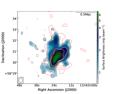
Figure 2: GMRT 610 MHz low-resolution color image with restoring beam $22.46\arcsec\times 19.88\arcsec$, P.A $14.03\degree$ overlapped with VLA low resolution image contours in red and GMRT low-resolution image contours in black. The contours levels for GMRT are placed at $(-1,1,2,3,4,5,6)\times 3\sigma_{\mathrm{rms}}$ where $\sigma_{\mathrm{rms}}=260\ \mu$Jy/beam. Negative contours are dashed. The VLA contours are placed at levels $(1,2,3,4,5,6)\times 3\sigma_{\mathrm{rms}}$ where $\sigma_{\mathrm{rms}}=50\ \mu$Jy/beam. The white and yellow dashed lines shows the shape of the ridge region at 610 MHz and 1.4 GHz respectively. The yellow cross marks the location of cluster center from B14.

A1351 was observed with VLA A array during April 1994 (project code AB0699) in dual polarisation mode with 30 min on-source time. It was also observed with VLA C and D configuration in dual polarisation mode on April 2000 (project code AO0149) for 125 min and March 1995 (project code AM0469) for 15 min respectively. The observational summary is presented in Table  2. Common astronomy Software Aplication (CASA) was used for the data analysis. At first, the data for different configurations were treated individually for RFI removal and calibration. 3C286 was used as flux calibrator for all three configurations, and the flux density was set using the model described in Scaife & Heald (2012). After calibration was applied, the target data were split into new measurement sets for each of the data sets, and a few rounds of phase-only self-calibration were performed on the split measurement sets for all the configurations. The beam size and RMS reached using uniform weighting is given in Table  2. The weights of the three data sets were equalized using CASA task statweight, and then finally, the self-calibrated data sets were combined using CASA task concat for further imaging.

2.2.1 Imaging Diffuse Emission at 1.4 GHz:

We made a high-resolution image with the combined data using Briggs robust parameter -1. To get the diffuse emission, the individual point source emissions were masked from the high resolution image and then subtracted from the visibility data as explained previously. Finally, after subtraction of flux contribution from individual point sources, the image for diffuse emission was made using Briggs robust 0 and selecting a uv-range below 20 k$\lambda$ and using 5 k$\lambda$ uv-taper (Figure 2 red contours).

3 Results from Radio Observation

In this section, we discuss the results from GMRT 610 MHz and VLA 1.4 GHz radio Data. We also show the spectral index distribution of the diffuse emission.

3.1 GMRT 610 MHz

Optical study showed the cluster has two main sub-cluster in the northern region surrounding the two brightest cluster galaxies BCG1 and BCG2 (B14). BCG1 also coincides with the X-ray peak. Figure 1 (left panel) is the high-resolution radio image of the cluster, made using uniform weighting, overlaid on the optical image from SDSS DATA Release 12 (Alam et al., 2015). BCG1 and few other galaxies are vissible in radio band, but BCG2 does not have visible radio emission. The source TG in Figure 1 (left) is a tailed radio galaxy.

Figure 2 represents the low-resolution image of the diffuse emission after subtraction of the individual galaxies, overlapped with VLA red contours and GMRT black contours. The radio-bright edge, or the ridge (as mentioned in G09 and B14), has a Largest Linear Size (LLS) of $\sim$ 570 kpc with an elongation in the north-west south-east direction and a width of 260 kpc at 610 MHz. The shape of the bright ridge at 610 MHz has been highlighted with white dashed contour in Figure 2. The brightest region of the edge is located $\sim$ 470 kpc away from BCG1 and $\sim$ 290 kpc away from source TG.

3.1.1 Integrated Flux Density Estimation:

For estimation of integrated Flux density of the total diffuse emission of the cluster, we selected the region within the $3\sigma_{\mathrm{rms}}$ contour of Figure 2. The flux density within that contour region for GMRT 610 MHz was found to be $86.67\pm 5.49$ mJy where $\sigma_{\mathrm{rms}}=260\ \mu$Jy/beam. For calculating the uncertainty in flux density estimation, we used the equation

$$\Delta S=\sqrt{(\sigma_{\mathrm{cal}}\ S)^{2}+(\sigma_{\mathrm{rms}}\sqrt{N_{\mathrm{beam}}})^{2}}$$ (1)

where an uncertainty of 6% was assumed due to calibration error($\sigma_{\mathrm{cal}}$) following Chandra et al. 2004, ${N_{\mathrm{beam}}}$ is number of beams within the $3\sigma_{\mathrm{rms}}$ contour for GMRT image where $\sigma_{\mathrm{rms}}$ is the image RMS noise. The flux density of the radio edge (within 9$\sigma_{\mathrm{rms}}$ contour) was found 42.20 $\pm$ 2.68 mJy.
To crosscheck the value of flux density of the entire diffuse emission, we attempted another approach as described in Raja et al. (2020). In this approach, the flux densities of the galaxies were estimated from the high-resolution image (left panel, Figure 1) using PyBDSF (Python Blob Detector and Source Finder) (Mohan & Rafferty, 2015). Furthermore, these flux density values were subtracted from the total emission within the $3\sigma_{\mathrm{rms}}$ contour to get the amount of flux density from diffuse emission. We found the integrated flux density in this approach to be 87.18 $\pm$ 6.11 mJy.

3.2 VLA 1.4 GHz

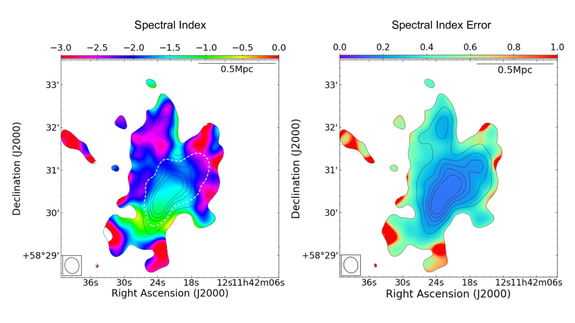
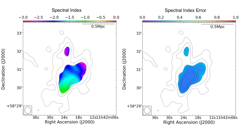
Figure 3: Top (Left): Spectral index map between 1.4 GHz and 610 MHz with beam $22.46\arcsec\times 19.88\arcsec$, P.A. $14.03\degree$ overlapped with GMRT low-resolution image contours in Black. The contours levels for GMRT are placed at $(1,2,3,4,5,6)\times 3\sigma_{\mathrm{rms}}$ where $\sigma_{\mathrm{rms}}=260\ \mu$Jy/beam. The edge region has been highlighted with white dashed contour. Bottom (Left): Spectral index map highlighting only the edge region. Top (Right): spectral index error map between 1.4 GHz and 610 MHz. Bottom (Right): spectral index error map for only the edge region.

The red contours in Figure 2 represent low-resolution images obtained with VLA 1.4 GHz observation. The diffuse emission is more extented in the northern region surrounding BCG1 and BCG2 at 1.4 GHz. This emission, classified as halo previously by G09, has a quite asymmetric and elongated structure. We have estimated the flux density of diffuse emission within $3\sigma_{\mathrm{rms}}$ contour to be $24.10\pm 2.44$ mJy where $\sigma_{\mathrm{rms}}=50\ \mu$Jy/beam. We used the same equation (equation 1) for estimating error in flux density measurement assuming 10% uncertainity due to calibration error. The flux density of the radio-bright ridge (highlighted with yellow dashed contour in Figure 2) was estimated to be 10.85 $\pm$ 1.10 mJy, which gave a radio luminosity $P_{1.4\mathrm{\ GHz}}=4.46\pm 0.61\times 10^{24}$ W $Hz^{-1}$. The luminosity was calculated using equation 2.

$$P_{1.4\mathrm{\ GHz}}=\frac{4\pi D_{L}^{2}(z)}{(1+z)^{(\alpha+1)}}\times S_{1.4\mathrm{\ GHz}}$$ (2)

Where $D_{L}(z)$ is luminosity distance at the redshift $z$. This estimation of radio luminosity is as per the radio luminosity estimated by G09 for the radio ridge region.

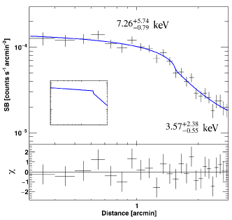
Figure 4: Left: Chandra X-ray surface brightness map of A1351 overlaid with GMRT 610 MHz low resolution image contours (black) and VLA 1.4 GHz low resolution image contours (cyan) with restoring beam $22.46\arcsec\times 19.88\arcsec$, P.A. $14.03\degree$. The contours levels are placed at levels (-1,1,2,3,4,5,6)$\times 3\sigma_{\mathrm{rms}}$ where $\sigma_{\mathrm{rms}}=260\ \mu$Jy/beam for 610 MHz image and $\sigma_{\mathrm{rms}}=50\ \mu$Jy/beam for 1.4 GHz image. The negative contours are dashed. The wedge region (magenta) was used to produce surface brightness profile, dashed regions (Blue) T1 and T2 are used to estimate the temperature across the discontinuity. The arc between the T1 and T2 region represents the position of the discontinuity. Right: The surface brightness profile over the wedge region (magenta, in the left panel). The inset shows the simulated gas density model. The Temperatures measured in T1 and T2 regions are $T_{1}=3.57^{+2.38}_{-0.55}$ keV and $T_{2}=7.26^{+5.74}_{-0.79}$ keV.

3.3 Spectral Index Estimation

To measure the spectral index, we made images with the same uv-range and the same restoring beam at the two frequencies. Generally, the diffuse emissions have a wider spread in the low-frequency domain. However, the northern section of the halo is not noticeable in the Figure 2 owing to the lesser sensitivity of the low-resolution image of 610 MHz. So, for spectral index estimation, the common region having diffuse emission present in both the frequencies was selected using CASA polygon drawing, and the flux densities in the region were noted. The spectral index was estimated using equation $\alpha=log(S_{1}/S_{2})/log(\nu_{1}/\nu_{2})$ where S and $\nu$ denotes flux densities at different frequencies and frequencies respectively. The integrated spectral index of the entire radio structure was found to be $\alpha_{\mathrm{total}}=-1.72\pm 0.33$, where the error in the spectral index was calculated using the equation 3.

$$\Delta\alpha=\frac{1}{\rm{log}(\nu_{1}/\nu_{2})}\times\sqrt{\frac{(\Delta S_{1})^{2}}{S_{1}^{2}}+\frac{(\Delta S_{2})^{2}}{S_{2}^{2}}}$$ (3)

We found the edge has a steep spectra with integrated spectral index $\alpha=-1.63\pm 0.33$.

3.3.1 Spectral Index Map:

Spectral index mapping is an essential and informative aspect of radio data analysis as it helps better understand the particle acceleration process in the cluster. The spectral index distribution can give us an idea of where the particles are recently accelerated, thus indicating shock acceleration/re-acceleration scenarios. The spectral index of freshly accelerated particles is flatter, and it steepens as the particles lose energy post acceleration. To make the spectral index map between 610 MHz and 1.4 GHz, we made images in each frequency with Brigg’s robust 0 (Briggs 1995), choosing the same uv-range of 20 k$\lambda$ and applying uv-taper of 5 k$\lambda$ in both cases. This choice of uv-range and tapering brought out the diffuse emission best in both frequencies. The final images were obtained with the same resolution of $22.46\arcsec\times 19.88\arcsec$, PA $14.03\degree$, with the same image size and cell size. The low-frequency image was regridded using the CASA task imregrid. The emission has less spread in some regions at 610 MHz (Figure  2). So the surface brightness below $3\sigma_{\mathrm{rms}}$ level of the GMRT 610 MHz images was masked. This masked region was copied to choose the same region from VLA 1.4 GHz image. Finally, the spectral index for each pixel was calculated using the CASA tool immath. The error in the spectral index was also calculated for each pixel (Figure 3).
Furthermore, we made the spectral index map of the bright edge/ridge region particularly, following the same way and choosing a surface brightness mask below $9\sigma_{\mathrm{rms}}$ level of the GMRT 610 MHz image. In Figure 3, a gradient of the spectral index can be observed along the south to north direction of the edge. This gradient resembles the shock downstream steepening of the spectral index for radio relics, where when a shock passes through ICM, it accelerates or re-accelerates the electrons to relativistic speed. At the location of the shock front, as the particles are recently accelerated, the diffuse emission gives relatively flatter spectra. In the post-shock region, the high-energy particles lose energy faster through synchrotron losses and the inverse Compton effect, so a steepening in the spectral index is noticed (Gennaro et al., 2018; Rajpurohit et al., 2020a).

3.4 Radio Mach Number

In the DSA model of particle acceleration, the particles from the thermal pool of ICM travel back and forth in the pre and post-shock region and gain energy in this process (Hoeft & Brüggen, 2007; Brunetti & Jones, 2014). This model predicts that the shock Mach number for planar shock $\mathcal{M}$ is related to the integrated spectral index over a region with different plasma ages as

$$\mathcal{M}_{\alpha}=\sqrt{\frac{(\alpha-1)}{(\alpha+1)}}$$ (4)

For the bright ridge/edge in A1351 we found a shock Mach number of 2.05 considering the integrated spectral index $\alpha$ = -1.63 over the region that shows spectral steepening similar to radio relics (Fig 3 Bottom Left).

4 Chandra X-ray Observation

We analyzed archival Chandra X-ray observations (ObsId 15136) of A1351. The total 33 ksec observations were taken in VFAINT mode. For this study, we employed a systematic calibration and analysis pipeline, which uses the Chandra Interactive Analysis of Observations (CIAO) and subsequent scripts in IDL and python. The details of our data reduction pipeline are described in (Datta et al., 2014; Schenck et al., 2014; Hallman et al., 2018; Raja et al., 2020; Rahaman et al., 2021), which initially consisted of several bash and IDL scripts. As A1351 is a comparatively low redshift cluster ($z=0.325$), the extended X-ray emission spills over all four ACIS-I chips. Therefore, we were not able to use the local background (as in, e.g., Raja et al. 2020). Hence, we subtracted the background contribution present in the observation by extracting background spectra from the ”blank-sky” background files. These ‘blank-sky’ background files are available in the Chandra calibration database (CALDB), which represents particle background and unresolved cosmic X-ray background. The “blank-sky” background was re-normalized in the 9.5 - 12 keV band. The Chandra effective area is negligible in the 9.5 - 12 keV band, and all the 9.5 - 12 keV flux in the sky data is due to particle background (Hickox & Markevitch, 2006).

Table 3: Best fit parameters of broken power law model (using PROFFIT) are listed below.

$\alpha 1$	$\alpha 2$	$r_{\mathrm{sh}}$(arcmin)	norm	Jump ($C$)	$\chi^{2}/D.o.f$	$\mathcal{M}_{\mathrm{SB}}$
0.16 $\pm$ 0.14	2.01 $\pm$ 0.35	1.55 $\pm$ 0.01	$5.43\pm 2.02e-05$	1.24 $\pm$ 0.25	15.80/18 (0.88)	$1.34^{+0.20}_{-0.19}$

Next, we removed point sources from the data by providing SAOImage DS9 region file containing point sources. These point sources were detected using the tool wavdetect inbuilt into CIAO in the 0.7 - 8.0 keV band with the scales of 1, 2, 4, 8, and 16 pixels. These were further inspected visually for any false detection or if wavdetect failed to detect any real point sources. Regions with point sources were removed from both data and blank-sky background files to avoid negative subtraction. After removing the point sources, we created light curves for individual ObsId in full energy and 9.5 - 12 keV bands. Light curves were binned at 259 seconds per bin for data as well as blank-sky backgrounds, and count rates higher than 3$\sigma$ were removed (background flares) using the deflare tool. These steps produced calibrated and clean data free from bad events as well as contaminating point sources.

After cleaning the data, we used merge_obs with binning 4 to produce a surface brightness map. The exposure corrected, background and point sources subtracted, 0.7 - 8.0 keV surface brightness image is shown in Figure 4.

We performed spectral analysis using XSPEC version: 12.9.1 (Arnaud, 1996) in between 0.7 - 8.0 keV energy range. We used CIAO task dmextract to create spectra from each region from each observations and specextract to calculate Auxiliary Response File (ARF) and Redistribution Matrix File (RMF). The APEC (Astrophysical Plasma Emission Code) and PHABS (PHotoelectric ABsorption) models were fitted to the spectra from each region using C-statistics (Cash, 1979). The metallicity of the cluster was kept frozen at 0.3 $Z_{\odot}$ throughout the cluster, where $Z_{\odot}$ is the solar abundance (Anders & Grevesse, 1989). Redshift (0.325; B14) and $N_{\mathrm{H}}$ ($7.12\times 10^{19}\mathrm{cm^{-2}}$; HI4PI Collaboration et al. 2016) were also kept frozen. Only APEC normalization and temperature were fitted for each region.

5 Results from X-ray Observation

Figure 4 shows the X-ray emission from the cluster is slightly elongated towards the N-NE S-SW direction, which implies a merging cluster B14. The cluster also hosts a large-scale diffuse radio emission (a radio halo and a radio bright edge/ridge). The contour of the radio edge is denser towards the southwest direction. These denser contours may have resulted due to compression by a shock front. Therefore, to look for a possible hint of cluster shock, we analyzed the cluster X-ray surface brightness profiles using PROFFIT v1.5 (Eckert et al., 2011; Eckert, 2016).

5.1 X-ray Surface Brightness Discontinuity:

To estimate any discontinuity in surface brightness profile, we proceeded in the following way. We created a number of concentric annuli over the wedge region with $6\arcsec$ bin size. This bin size was chosen to get a sufficient count in each bin. We iteratively choose the wedge region to maximize the jump of the surface brightness discontinuity. The surface brightness profile over the wedge region was fitted with a broken power-law model (bknpow, in-build in PROFFIT v1.5). The broken power-law density model can be defined as

$$\begin{split}n(r)&=Cn_{0}\Big{(}\frac{r<r_{\mathrm{sh}}}{r_{\mathrm{sh}}}\Big{)}^{-\alpha 1}\\ &=n_{0}\Big{(}\frac{r>r_{\mathrm{sh}}}{r_{\mathrm{sh}}}\Big{)}^{-\alpha 2}\end{split}$$ (5)

where $C$ is the compression factor, $n(r)$ is electron number density, $n_{0}$ is normalization constant, $r_{\mathrm{sh}}$ is the radial distance of the shock, $r$ is the distance from the center of the wedge region, and $\alpha 1$ and $\alpha 2$ are the power-law indices for the respective profiles. We found a discontinuity in the surface brightness profile over the wedge region (magenta) shown in Figure 4. The best-fitted parameters and the profile is shown in Table 3 and Figure 4 (right panel) respectively. The position of the discontinuity in surface brightness is shown with an arc between the T1 and T2 regions in the left panel of Figure 4. The broken power law was fitted with a reduced $\chi^{2}$ value of 0.88.

5.2 X-ray Temperature Jump:

To characterize the surface brightness discontinuity as shock or cold front, we estimated the temperature across the regions of the discontinuity. As the exposure of the Chandra observation was short, we were not able to make a temperature profile, but from the dedicated regions across the discontinuity (e.g., T1 and T2 in Figure 4). We iteratively choose the width of the region to have threshold counts in the corresponding spectra. We took regions with 41$\arcsec$ of width, labeled as T1 and T2 in the left panel of Figure 4. The temperature was estimated by fitting the thermal APEC and PHABS model as discussed in section 4. The estimated temperatures in the pre-shock or upstream region, $T_{1}$ and post-shock or downstream region, $T_{2}$ are listed in Table 4, where $T_{1}$ and $T_{2}$ are temperatures from the regions T1 and T2 respectively as labeled in Figure 4 (left panel). We found that there is a significant jump in the temperature along the direction similar to the surface brightness discontinuity. Therefore, the presence of both discontinuities hints towards the shock front.

Table 4: Shock upstream (T₁) and downstream T₂ temperatures and Mach number from temperature jump is listed below.

T1(Tup)	T2(Tdown)	$\mathcal{M}_{\mathrm{T}}$
$3.57^{+2.38}_{-0.55}$ keV	$7.26^{+5.74}_{-0.79}$ keV	$1.96^{+1.36}_{-0.86}$

5.3 X-ray Mach Numbers

Assuming the jumps as shock front, we calculated the Mach number using the Rankine-Hugoniot shock jump condition given as

$$\frac{\rho_{2}}{\rho_{1}}=C=\frac{(1+\gamma)\times\mathcal{M}_{\mathrm{SB}}^{2}}{2+(\gamma-1)\times\mathcal{M}_{\mathrm{SB}}^{2}}$$ (6)

where $\rho_{1}$ & $\rho_{2}$ are densities at pre and post shock region respectively and for mono-atomic gas, considering $\gamma=5/3$, we get

$$C=\frac{4\mathcal{M}_{\mathrm{SB}}^{2}}{3+\mathcal{M}_{\mathrm{SB}}^{2}}$$ (7)

This gives a shock Mach number from density jump across the shock edge, $\mathcal{M}_{SB}=1.34^{+0.20}_{-0.19}$.
The Mach number from temperature jump was calculated using Rankine-Hugoniot temperature jump condition

$$\frac{T_{2}}{T_{1}}=\frac{(5\mathcal{M}_{\mathrm{T}}^{2}-1)(\mathcal{M}_{\mathrm{T}}^{2}+3)}{16\mathcal{M}_{\mathrm{T}}^{2}}$$ (8)

where, $T_{1}$ and $T_{2}$ are the pre-shock (upstream) and post-shock (downstream) temperature respectively (Table 4). The Mach number from temperature jump was found to be $\mathcal{M}_{\mathrm{T}}=1.96^{+1.36}_{-0.86}$.

6 Discussion

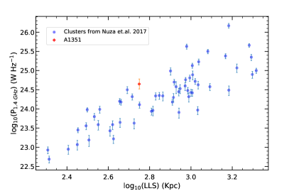
Figure 5: Radio Luminosity $P_{1.4\ \mathrm{GHz}}$ vs. Largest Linear Size (LLS) of the relics adopted from the literature (Nuza et al. 2017). The relic in A1351, marked with a red diamond, follows observed trend and given its size, it is one of the highly luminous relics.

The diffuse radio emission in A1351 is quite asymmetric in nature with the presence of the bright region at the southern part of the radio halo (Figure 2). This type of radio-bright edges within radio halos has been noticed previously for a few clusters but with smaller sizes (e.g. Markevitch et al. 2005; Macario et al. 2011; Shimwell et al. 2014; Wang et al. 2018). Here, the bright edge has an LLS of $\sim$570 kpc at 610 MHz and situated at a distance of $\sim$470 kpc away from the cluster center. This size and location indicate that the edge can be a relic. As mentioned in B14, the cluster is undergoing a merging in the N-NE S-SW direction where the passage of an axial shock can form the relic. The spectral index distribution in A1351 is in agreement with the other reported cases where cluster radio shocks resulted in radio relics in cluster peripheral region (see review by van Weeren et al. 2019). We have compared the LLS and luminosity ($P_{1.4\ \mathrm{GHz}}$) of the relic in A1351 with other known relics from Nuza et al. 2017 (Figure 5). We see that the relic in A1351 (Marked in Red diamond) follows the observed trend in $P_{1.4\ \mathrm{GHz}}$-LLS plot. Given its LLS, The relic is one of the highly luminous relics with a radio power $P_{1.4\ \mathrm{GHz}}$ = $4.46\times 10^{24}$ W $Hz^{-1}$.

For the case of A1351, the shock Mach number derived from Radio observation ($\mathcal{M}_{\alpha}$ = 2.05) is slightly higher than that observed from the X-ray temperature jump ($\mathcal{M}_{T}$ = $1.96^{+1.36}_{-0.86}$) and density jump ($\mathcal{M}_{SB}$ = $1.34^{+0.20}_{-0.19}$). The discrepancy is expected as the radio synchrotron emission is dependent on the amplitude of the magnetic field fluctuations. These fluctuations decrease slower than the density and temperature fluctuations leading to the higher values of radio-derived Mach number seen for most radio relics (Domí nguez-Fernández et al., 2020). Wittor et al. (2021) showed the radio-derived Mach numbers are more skewed to the higher value of Mach number distribution while the X-ray derived Mach numbers reflect their average distribution. Moreover, the discrepancy observed in the derived values of Mach numbers is due to the systematic errors that can affect the different analyses. The radio estimations can suffer errors in flux measurement due to shallow data or source contamination (Hoang et al., 2017). Also, the measurement of Mach number from spectral index is challenging. Mach number measured using the injection index close to the shock front is theoretically more precise in determining the shock properties. However, it is more difficult to achieve as it needs identification of the position of the shock precisely. An experimentally more robust approach to Mach number is using the volume-averaged spectral index. Although, this approach is theoretically less precise as it involves electrons from different ages across the relic (Colafrancesco et al., 2017; Wittor et al., 2021). On the other hand, the influence of the projection effect on X-ray analyses makes the radio findings a more robust technique (Hong et al., 2015; Akamatsu et al., 2017). In case of temperature estimation, there is the possibility of both underestimating the post-shock temperature as well as overestimating the pre-shock temperature, which can lead to underestimation of Mach number ($\mathcal{M}_{T}$). However, the temperature jump is still less subject to the projection effect than the density jump and thus the former one gives a more reliable result (Ogrean et al., 2013; Akamatsu et al., 2017).

In our case, the value of the shock Mach number obtained from radio observation is quite consistent with the shock Mach number derived from the X-ray temperature jump. This supports the DSA mechanism of particle acceleration at the shock front. The spectral index gradient is also in accordance with that. There have been very few radio relics in the literature where DSA mechanism for particle acceleration with weak shocks could be established (Bourdin et al., 2013; Shimwell et al., 2015; Botteon et al., 2016b; Locatelli et al., 2020; Rajpurohit et al., 2021). The relic in A1351 is a viable candidate for supporting DSA.

6.1 Electron acceleration efficiency

The LLS - P${}_{1.4\ \mathrm{GHz}}$ graph (Figure 5) shows that the relic in A1351 is highly luminous, which would require high acceleration efficiency for the thermal electrons. To check the consistency of the DSA model and the electron acceleration efficiency needed to produce the observed radio luminosity for A1351, we used the relationship as described in Hoeft et al. 2008; Locatelli et al. 2020. The acceleration efficiency $\zeta_{e}$ is related to the cluster magnetic field B, X-ray properties, and radio luminosity $P_{\nu}$ at frequency $\nu$ by the equation

$$\zeta_{e}=\frac{P_{\nu}}{6.4\times 10^{-34}}\frac{B^{2}+B_{\mathrm{CMB}}^{2}}{B^{1-\frac{\alpha}{2}}}\frac{\mathrm{Mpc^{2}}}{A}\Big{(}\frac{\nu}{1.4\ \mathrm{GHz}}\Big{)}^{\frac{-\alpha}{2}}\\ \Big{(}\frac{7\ \mathrm{keV}}{T_{\mathrm{d}}}\Big{)}^{\frac{3}{2}}\frac{10^{-4}}{n_{\mathrm{ed}}}$$ (9)

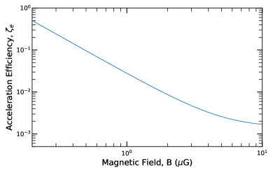
Figure 6: The electron acceleration efficiency $\zeta_{e}$ plotted against magnetic field at the shock location. The value of the magnetic field has been kept within few $\mu$G.

Where $\alpha$ is the spectral index -1.63, $T_{\mathrm{d}}$ is the downstream temperature $7.26^{+5.74}_{-0.79}$ keV, $n_{\mathrm{ed}}$ is the downstream electron density [$0.26^{+0.12}_{-0.15}\ \times\ 10^{-3}$] cm^-3 and $B_{\rm CMB}$ is the equivalent magnetic field of Cosmic Microwave Background at the cluster redshift. The surface area, $A$ of the relic was taken as LLS $\times$ LLS following (Locatelli et al., 2020; Rajpurohit et al., 2020b). $B_{\rm CMB}$ was evaluated at redshift 0.325 using the equation 10 following Hoeft & Brüggen 2007.

$$B_{\mathrm{CMB}}=3.24(1+z)^{2}\mu G$$ (10)

Figure 6 shows that in the presence of a few $\mu$G magnetic fields (0.5 - 5 $\mu$G), the efficiency $\zeta_{e}$ at the shock location varies from $\sim 10\%$ to $\sim 0.2\%$. This range of acceleration efficiency is comparable to other cases where DSA model could explain the observed luminosity of the respective radio relics (e.g. A521, El Gordo Botteon et al. 2020). The high luminosity and the weak shock with $\mathcal{M}\sim 2.05$ raise the possibility that DSA might not be the sole mechanism for powering the relic and that shock re-acceleration might be involved as well. However, in presence of a strong magnetic field, the acceleration of thermal electrons via the DSA is still a possible option for the relic in A1351. Deeper observations are required to shed more light about the particle acceleration process.

6.2 Equipartition Magnetic Field

Cluster magnetic field can be approximated assuming equipartition of energy between cosmic ray particle and magnetic field (Govoni & Feretti 2004; Bonafede et al. 2009a; van Weeren et al. 2009; Parekh et al. 2020; Pandge et al. 2022). To quantify the magnetic field at the relic location in A1351, we assumed that the system satisfies minimum energy density condition. The minimum energy density $u_{\mathrm{min}}$ is obtained using equation 11 following Govoni & Feretti 2004.

$$u_{\mathrm{min}}=\xi(-\alpha,\nu_{1},\nu_{2})(1+k)^{\frac{4}{7}}(\nu_{0})^{\frac{-4\alpha}{7}}(1+z)^{\frac{12-4\alpha}{7}}\Big{(}\frac{I_{0}}{d}\Big{)}^{\frac{4}{7}}$$ (11)

Where $\xi(-\alpha,\nu_{1},\nu_{2})=1.57\times 10^{-13}$ for a frequency range $\nu_{1}$(10 MHz) - $\nu_{2}$(100 GHz) and spectral index $\alpha$ = -1.63 (Govoni & Feretti, 2004), $\nu_{0}$ = 1400 MHz, $I_{0}$ was estimated by dividing the flux density (10.82 mJy) of the relic at 1.4 GHz by the solid angle of $85\arcsec\times 103\arcsec$, and the depth $d$ of the relic was obtained in kpc taking an average of the largest (550 kpc at 1.4 GHz) and smallest (220 kpc at 1.4 GHz) linear size of the relic at 1.4 GHz. We assumed the ratio of the energy content of cosmic-ray protons and electrons $k=1$ (Parekh et al., 2020). Thereafter, the equipartition magnetic field $B_{\mathrm{eq}}$ can be found using equation 12

$$B_{\mathrm{eq}}=\Big{(}\frac{24\pi}{7}u_{\mathrm{min}}\Big{)}^{1/2}$$ (12)

The magnetic field found with this approach at A1351’s relic location is $\sim$ 1.8 $\mu$G.

A modified formula to compute the magnetic field strength of synchrotron radio sources ($B\arcmin_{\mathrm{eq}}$) is to consider an upper and lower energy cut-offs for the cosmic ray electrons rather than frequency cut-offs (Brunetti et al., 1997; Beck & Krause, 2005). Assuming $\gamma_{\mathrm{min}}=100\ (<<\gamma_{\mathrm{max}})$, the revised magnetic field is calculated using equation 13.

$$B\arcmin_{\mathrm{eq}}\sim 1.1\gamma_{\mathrm{min}}^{\frac{1+2\alpha}{3-\alpha}}B_{\mathrm{eq}}^{\frac{7}{2(3-\alpha)}}$$ (13)

Where $\gamma$ is the Lorentz factor, $B_{\mathrm{eq}}$ is the equipartion magnetic field obtained using equation 12. The revised magnetic field found for A1351 relic is $\sim 5.3\ \mu$G. The equipartition theory relies on several assumptions. The particle energy distribution at the cluster is poorly known. Projection effects can influence the extent of the relic, and the assumption of the relic’s depth can affect the derived value of magnetic field. A better constraint on the magnetic field can be given through Faraday Rotation Measure (RM). For few radio relics, the magnetic field derived using RM study are in agreement with equipartition estimation (eg. coma cluster: Bonafede et al. 2013, MACSJ0717.5$\pm$3745: Bonafede et al. 2009c; Rajpurohit et al. 2022 ). However, for few cases the magnetic fields derived from these two methods differ (eg. A2345: Bonafede et al. 2009b; Stuardi et al. 2021; A3667: Johnston-Hollitt 2003; de Gasperin et al. 2021). Polarisation study is needed to give a better estimation of the magnetic field.

7 Summary

In this paper, we present the first time analysis and result of GMRT 610 MHz, Chandra X-ray data of A1351 and a reanalysis of the VLA 1.4 GHz data to understand the origin of the peculiar radio edge emission present in the cluster. With Chandra data we searched for any possible hint of shock at the location of the bright radio edge in A1351. Our findings are summerized below.

• From radio observation, we measured a total diffuse emission flux at 610 MHz and 1.4 GHz to be $86.67\pm 5.49$ mJy and $24.10\pm 2.44$ mJy, respectively. The average spectral index of the cluster diffuse emission was found to be $\alpha_{\mathrm{total}}=-1.72\pm 0.33$. The bright edge of the cluster has an LLS of $\sim$ 570 kpc at 610 MHz, radio luminosity $P_{1.4\ \mathrm{GHz}}$ = $4.46\times 10^{24}$ W $\mathrm{Hz}^{-1}$ and an integrated spectral index $\alpha=-1.63\pm 0.33$ giving a Mach number $\mathcal{M}_{\alpha}$ = 2.05. The spectral index map shows a spectral index gradient at the edge location.

• Using Chandra observation, we found the presence of shock at the location of the edge. The shock Mach numbers found from X-ray temperature and density jumps are $1.96^{+1.36}_{-0.86}$ and $1.34^{+0.20}_{-0.19}$, respectively.

• Its larger size, gradient in the spectral index map, and position of the X-ray shock support the idea that the edge is a radio relic. The relic follows the $P_{1.4\ \mathrm{GHz}}$-LLS trend with other observed relics from the NVSS survey and stands as one of the powerful relics considering its size.

• We found a magnetic field of $\sim 5.3\ \mu$G in the relic’s location assuming equipartition. In presence of this high magnetic field, it is very likely that the relic in A1351 might have originated from DSA of thermal electrons. The formation of this highly luminous relic in presence of weak shock makes it one of the unique cases which can unfold interesting information about cluster scale acceleration processes.

• Future deep X-ray observation can help us study the cluster X-ray morphology in more detail. Future polarisation study can give better understanding of the cluster magnetic field. Multi-frequency radio observations are needed to search for spectral curvature and also to study this halo relic system in more detail.

Data Availability

The archival radio data used in our work are available in the GMRT Online archive (https://naps.ncra.tifr.res.in/goa/data/search, project code 17_019),the VLA Data Archive (https://archive.nrao.edu/archive/advquery.jsp, project codes AB0699, AO0149 and AM0469) and the Chandra data archive (https://cda.harvard.edu/chaser/, ObsId 15136)

Appendix A X-ray surface brightness profile over SE wedge region

To check the reliability of the surface brightness discontinuity detected in the southwest (SW) region of A1351, we created another similar profile along the southeast (SE) region (see Figure 7, left panel). We fitted the profile of this wedge region with broken power law (Figure 7, middle) but no density or temperature jump was observed over the wedge region. Figure 7, right panel shows a power law fit over the profile. The fitting parameters are mentioned in Table 5. Unlike the SW profile, the SE profile shows no discontinuity. Therefore, we argue that the discontinuity in the SW profile (shown in Figure 4) might be caused by the merging shock.

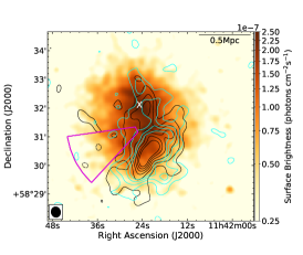
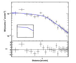
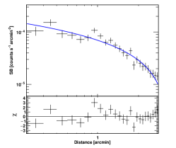
Figure 7: Left: Chandra X-ray surface brightness map of A1351 overlaid with 610 MHz GMRT low resolution image contours (black) and VLA 1.4 GHz low resolution image contours (cyan) with restoring beam $22.46\arcsec\times 19.88\arcsec$, P.A. $14.03\degree$. The contours levels are placed at levels (-1,1,2,3,4,5,6) $\times\ 3\sigma_{\mathrm{rms}}$ where $\sigma_{\mathrm{rms}}=260\mu$Jy/beam for 610 MHz image and $\sigma_{\mathrm{rms}}=50\mu$Jy/beam for 1.4 GHz image. The wedge region (magenta) was used to produce a surface brightness profile. Middle: X-ray surface brightness profile obtained from the wedge region (magenta) shown in the left panel. This profile was fitted with a broken power law, but no discontinuity ($C=0.92\pm 0.15$) was detected. Right: X-ray surface brightnes profile fitted with Power law.

Table 5: Best fit parameters of broken power law model (using PROFFIT) are listed below.

Model	$\alpha 1$	$\alpha 2$	$r_{sh}$(arcmin)	norm	Jump(C)	$\chi^{2}/D.o.f$
Broken power law	0.19$\pm$0.18	1.30$\pm$ 0.13	1.15$\pm$0.01	$5.11\pm 0.82e-05$	0.92 $\pm$ 0.15	23.3/18 (1.29)
Power law	6.27 $\pm$ 3.29 e-02		3.95 $\pm$ 1.27	8.81 $\pm$ 4.5 e-04		32.37 / 20 (1.62)

References

- Akamatsu et al. (2017) Akamatsu, H., Mizuno, M., Ota, N., et al. 2017, A&A, 600, A100, doi: 10.1051/0004-6361/201628400
- Alam et al. (2015) Alam, S., Albareti, F. D., Allende Prieto, C., et al. 2015, ApJS, 219, 12, doi: 10.1088/0067-0049/219/1/12
- and A. M. Price-Whelan et al. (2018) and A. M. Price-Whelan, Sipőcz, B. M., Günther, H. M., et al. 2018, The Astronomical Journal, 156, 123, doi: 10.3847/1538-3881/aabc4f
- Anders & Grevesse (1989) Anders, E., & Grevesse, N. 1989, Geochim. Cosmochim. Acta, 53, 197, doi: 10.1016/0016-7037(89)90286-X
- Arnaud (1996) Arnaud, K. A. 1996, in Astronomical Society of the Pacific Conference Series, Vol. 101, Astronomical Data Analysis Software and Systems V, ed. G. H. Jacoby & J. Barnes, 17
- Astropy Collaboration et al. (2013) Astropy Collaboration, Robitaille, T. P., Tollerud, E. J., et al. 2013, A&A, 558, A33, doi: 10.1051/0004-6361/201322068
- Barrena et al. (2014) Barrena, R., Girardi, M., Boschin, W., De Grandi, S., & Rossetti, M. 2014, MNRAS, 442, 2216, doi: 10.1093/mnras/stu1011
- Beck & Krause (2005) Beck, R., & Krause, M. 2005, Astronomische Nachrichten, 326, 414, doi: 10.1002/asna.200510366
- Bohringer et al. (2000) Bohringer, H., Voges, W., Huchra, J. P., et al. 2000, The Astrophysical Journal Supplement Series, 129, 435–474, doi: 10.1086/313427
- Bonafede et al. (2009a) Bonafede, A., Giovannini, G., Feretti, L., Govoni, F., & Murgia, M. 2009a, A&A, 494, 429, doi: 10.1051/0004-6361:200810588
- Bonafede et al. (2009b) —. 2009b, A&A, 494, 429, doi: 10.1051/0004-6361:200810588
- Bonafede et al. (2013) Bonafede, A., Vazza, F., Bruggen, M., et al. 2013, Monthly Notices of the Royal Astronomical Society, 433, 3208
- Bonafede et al. (2009c) Bonafede, A., Feretti, L., Giovannini, G., et al. 2009c, A&A, 503, 707, doi: 10.1051/0004-6361/200912520
- Botteon et al. (2020) Botteon, A., Brunetti, G., Ryu, D., & Roh, S. 2020, A&A, 634, A64, doi: 10.1051/0004-6361/201936216
- Botteon et al. (2016a) Botteon, A., Gastaldello, F., Brunetti, G., & Dallacasa, D. 2016a, MNRAS, 460, L84, doi: 10.1093/mnrasl/slw082
- Botteon et al. (2016b) Botteon, A., Gastaldello, F., Brunetti, G., & Kale, R. 2016b, MNRAS, 463, 1534, doi: 10.1093/mnras/stw2089
- Botteon et al. (2022) Botteon, A., Shimwell, T. W., Cassano, R., et al. 2022, arXiv e-prints, arXiv:2202.11720. https://arxiv.org/abs/2202.11720
- Bourdin et al. (2013) Bourdin, H., Mazzotta, P., Markevitch, M., Giacintucci, S., & Brunetti, G. 2013, ApJ, 764, 82, doi: 10.1088/0004-637X/764/1/82
- Briggs (1995) Briggs, D. S. 1995, in American Astronomical Society Meeting Abstracts, Vol. 187, American Astronomical Society Meeting Abstracts, 112.02
- Brown & Rudnick (2011) Brown, S., & Rudnick, L. 2011, Monthly Notices of the Royal Astronomical Society, 412, 2, doi: 10.1111/j.1365-2966.2010.17738.x
- Brunetti & Jones (2014) Brunetti, G., & Jones, T. W. 2014, International Journal of Modern Physics D, 23, 1430007, doi: 10.1142/S0218271814300079
- Brunetti et al. (1997) Brunetti, G., Setti, G., & Comastri, A. 1997, A&A, 325, 898. https://arxiv.org/abs/astro-ph/9704162
- Cash (1979) Cash, W. 1979, ApJ, 228, 939, doi: 10.1086/156922
- Chandra et al. (2004) Chandra, P., Ray, A., & Bhatnagar, S. 2004, ApJ, 612, 974, doi: 10.1086/422675
- Colafrancesco et al. (2017) Colafrancesco, S., Marchegiani, P., & Paulo, C. M. 2017, MNRAS, 471, 4747, doi: 10.1093/mnras/stx1806
- Dahle et al. (2002) Dahle, H., Kaiser, N., Irgens, R. J., Lilje, P. B., & Maddox, S. J. 2002, ApJS, 139, 313, doi: 10.1086/338678
- Datta et al. (2014) Datta, A., Schenck, D. E., Burns, J. O., Skillman, S. W., & Hallman, E. J. 2014, ApJ, 793, 80, doi: 10.1088/0004-637X/793/2/80
- de Gasperin et al. (2021) de Gasperin, F., Rudnick, L., Finoguenov, A., et al. 2021, arXiv e-prints, arXiv:2111.06940. https://arxiv.org/abs/2111.06940
- Domí nguez-Fernández et al. (2020) Domí nguez-Fernández, P., Brüggen, M., Vazza, F., et al. 2020, Monthly Notices of the Royal Astronomical Society, 500, 795, doi: 10.1093/mnras/staa3018
- Drury (1984) Drury, L. O. 1984, Advances in Space Research, 4, 185, doi: 10.1016/0273-1177(84)90311-9
- Eckert (2016) Eckert, D. 2016, PROFFIT: Analysis of X-ray surface-brightness profiles. http://ascl.net/1608.011
- Eckert et al. (2011) Eckert, D., Molendi, S., & Paltani, S. 2011, A&A, 526, A79, doi: 10.1051/0004-6361/201015856
- Ensslin et al. (1998) Ensslin, T. A., Biermann, P. L., Klein, U., & Kohle, S. 1998, A&A, 332, 395. https://arxiv.org/abs/astro-ph/9712293
- Enßlin, T. A. & Gopal-Krishna (2001) Enßlin, T. A., & Gopal-Krishna. 2001, A&A, 366, 26, doi: 10.1051/0004-6361:20000198
- Enßlin & Brüggen (2002) Enßlin, T. A., & Brüggen, M. 2002, Monthly Notices of the Royal Astronomical Society, 331, 1011, doi: 10.1046/j.1365-8711.2002.05261.x
- Feretti et al. (2012) Feretti, L., Giovannini, G., Govoni, F., & Murgia, M. 2012, A&A Rev., 20, 54, doi: 10.1007/s00159-012-0054-z
- Ferrari et al. (2008) Ferrari, C., Govoni, F., Schindler, S., Bykov, A. M., & Rephaeli, Y. 2008, Space Sci. Rev., 134, 93, doi: 10.1007/s11214-008-9311-x
- Gennaro et al. (2018) Gennaro, G. D., van Weeren, R. J., Hoeft, M., et al. 2018, The Astrophysical Journal, 865, 24, doi: 10.3847/1538-4357/aad738
- Giacintucci et al. (2009) Giacintucci, S., Venturi, T., Cassano, R., Dallacasa, D., & Brunetti, G. 2009, ApJ, 704, L54, doi: 10.1088/0004-637X/704/1/L54
- Giovannini et al. (2009) Giovannini, G., Bonafede, A., Feretti, L., et al. 2009, A&A, 507, 1257, doi: 10.1051/0004-6361/200912667
- Govoni & Feretti (2004) Govoni, F., & Feretti, L. 2004, International Journal of Modern Physics D, 13, 1549, doi: 10.1142/S0218271804005080
- Hallman et al. (2018) Hallman, E. J., Alden, B., Rapetti, D., Datta, A., & Burns, J. O. 2018, ApJ, 859, 44, doi: 10.3847/1538-4357/aabf3a
- HI4PI Collaboration et al. (2016) HI4PI Collaboration, Ben Bekhti, N., Flöer, L., et al. 2016, A&A, 594, A116, doi: 10.1051/0004-6361/201629178
- Hickox & Markevitch (2006) Hickox, R. C., & Markevitch, M. 2006, ApJ, 645, 95, doi: 10.1086/504070
- Hoang et al. (2017) Hoang, D. N., Shimwell, T. W., Stroe, A., et al. 2017, MNRAS, 471, 1107, doi: 10.1093/mnras/stx1645
- Hoang et al. (2021) Hoang, D. N., Zhang, X., Stuardi, C., et al. 2021, arXiv e-prints, arXiv:2106.00679. https://arxiv.org/abs/2106.00679
- Hoeft & Brüggen (2007) Hoeft, M., & Brüggen, M. 2007, MNRAS, 375, 77, doi: 10.1111/j.1365-2966.2006.11111.x
- Hoeft et al. (2008) Hoeft, M., Brüggen, M., Yepes, G., Gottlöber, S., & Schwope, A. 2008, MNRAS, 391, 1511, doi: 10.1111/j.1365-2966.2008.13955.x
- Hong et al. (2015) Hong, S. E., Kang, H., & Ryu, D. 2015, ApJ, 812, 49, doi: 10.1088/0004-637X/812/1/49
- Hunter (2007) Hunter, J. D. 2007, Computing in Science & Engineering, 9, 90, doi: 10.1109/MCSE.2007.55
- Intema, H. T. et al. (2017) Intema, H. T., Jagannathan, P., Mooley, K. P., & Frail, D. A. 2017, A&A, 598, A78, doi: 10.1051/0004-6361/201628536
- Intema, H. T. et al. (2009) Intema, H. T., van der Tol, S., Cotton, W. D., et al. 2009, A&A, 501, 1185, doi: 10.1051/0004-6361/200811094
- Johnston-Hollitt (2003) Johnston-Hollitt, M. 2003, PhD thesis, University of Adelaide
- Kale et al. (2018) Kale, R., Parekh, V., & Dwarakanath, K. S. 2018, MNRAS, 480, 5352, doi: 10.1093/mnras/sty2227
- Kang & Ryu (2013) Kang, H., & Ryu, D. 2013, ApJ, 764, 95, doi: 10.1088/0004-637X/764/1/95
- Kempner et al. (2003) Kempner, J. C., Blanton, E. L., Clarke, T. E., et al. 2003, in The Riddle of Cooling Flows in Galaxies and Clusters of Galaxies. https://arxiv.org/abs/astro-ph/0310263
- Locatelli et al. (2020) Locatelli, N. T., Rajpurohit, K., Vazza, F., et al. 2020, MNRAS, 496, L48, doi: 10.1093/mnrasl/slaa074
- Macario et al. (2011) Macario, G., Markevitch, M., Giacintucci, S., et al. 2011, The Astrophysical Journal, 728, 82, doi: 10.1088/0004-637x/728/2/82
- Mandal et al. (2019) Mandal, S., Intema, H. T., Shimwell, T. W., et al. 2019, A&A, 622, A22, doi: 10.1051/0004-6361/201833992
- Markevitch et al. (2005) Markevitch, M., Govoni, F., Brunetti, G., & Jerius, D. 2005, ApJ, 627, 733, doi: 10.1086/430695
- Mohan & Rafferty (2015) Mohan, N., & Rafferty, D. 2015, PyBDSF: Python Blob Detection and Source Finder. http://ascl.net/1502.007
- Nuza et al. (2017) Nuza, S. E., Gelszinnis, J., Hoeft, M., & Yepes, G. 2017, MNRAS, 470, 240, doi: 10.1093/mnras/stx1109
- Ogrean et al. (2013) Ogrean, G. A., Brüggen, M., van Weeren, R. J., et al. 2013, MNRAS, 433, 812, doi: 10.1093/mnras/stt776
- Owen et al. (1999) Owen, F., Morrison, G., & Voges, W. 1999, in Diffuse Thermal and Relativistic Plasma in Galaxy Clusters, ed. H. Boehringer, L. Feretti, & P. Schuecker, 9
- Pandge et al. (2022) Pandge, M. B., Kale, R., Dabhade, P., Mahato, M., & Raychaudhury, S. 2022, MNRAS, 509, 1837, doi: 10.1093/mnras/stab2945
- Parekh et al. (2020) Parekh, V., Thorat, K., Kale, R., et al. 2020, MNRAS, 499, 404, doi: 10.1093/mnras/staa2795
- Rahaman et al. (2021) Rahaman, M., Raja, R., Datta, A., et al. 2021, MNRAS, 505, 480, doi: 10.1093/mnras/stab1225
- Raja et al. (2020) Raja, R., Rahaman, M., Datta, A., et al. 2020, ApJ, 889, 128, doi: 10.3847/1538-4357/ab620d
- Rajpurohit et al. (2020a) Rajpurohit, K., Hoeft, M., Vazza, F., et al. 2020a, A&A, 636, A30, doi: 10.1051/0004-6361/201937139
- Rajpurohit et al. (2020b) —. 2020b, aap, 636, A30, doi: 10.1051/0004-6361/201937139
- Rajpurohit et al. (2021) Rajpurohit, K., Vazza, F., van Weeren, R. J., et al. 2021, arXiv e-prints, arXiv:2104.05690. https://arxiv.org/abs/2104.05690
- Rajpurohit et al. (2022) Rajpurohit, K., Hoeft, M., Wittor, D., et al. 2022, A&A, 657, A2, doi: 10.1051/0004-6361/202142340
- Richard-Laferrière et al. (2020) Richard-Laferrière, A., Hlavacek-Larrondo, J., Nemmen, R. S., et al. 2020, Monthly Notices of the Royal Astronomical Society, 499, 2934–2958, doi: 10.1093/mnras/staa2877
- Robitaille & Bressert (2012) Robitaille, T., & Bressert, E. 2012, APLpy: Astronomical Plotting Library in Python. http://ascl.net/1208.017
- Sarazin (2002) Sarazin, C. L. 2002, Merging Processes in Galaxy Clusters, 1–38, doi: 10.1007/0-306-48096-4_1
- Scaife & Heald (2012) Scaife, A. M. M., & Heald, G. H. 2012, Monthly Notices of the Royal Astronomical Society: Letters, 423, L30, doi: 10.1111/j.1745-3933.2012.01251.x
- Schenck et al. (2014) Schenck, D. E., Datta, A., Burns, J. O., & Skillman, S. 2014, AJ, 148, 23, doi: 10.1088/0004-6256/148/1/23
- Shimwell et al. (2014) Shimwell, T. W., Brown, S., Feain, I. J., et al. 2014, MNRAS, 440, 2901, doi: 10.1093/mnras/stu467
- Shimwell et al. (2015) Shimwell, T. W., Markevitch, M., Brown, S., et al. 2015, MNRAS, 449, 1486, doi: 10.1093/mnras/stv334
- Slee et al. (2001) Slee, O. B., Roy, A. L., Murgia, M., Andernach, H., & Ehle, M. 2001, AJ, 122, 1172, doi: 10.1086/322105
- Stuardi et al. (2021) Stuardi, C., Bonafede, A., Lovisari, L., et al. 2021, MNRAS, 502, 2518, doi: 10.1093/mnras/stab218
- Stuardi et al. (2019) Stuardi, C., Bonafede, A., Wittor, D., et al. 2019, MNRAS, 489, 3905, doi: 10.1093/mnras/stz2408
- van Weeren et al. (2019) van Weeren, R. J., de Gasperin, F., Akamatsu, H., et al. 2019, Space Sci. Rev., 215, 16, doi: 10.1007/s11214-019-0584-z
- van Weeren et al. (2009) van Weeren, R. J., Röttgering, H. J. A., Bagchi, J., et al. 2009, A&A, 506, 1083, doi: 10.1051/0004-6361/200912287
- van Weeren et al. (2017) van Weeren, R. J., Andrade-Santos, F., Dawson, W. A., et al. 2017, Nature Astronomy, 1, 0005, doi: 10.1038/s41550-016-0005
- Wang et al. (2018) Wang, Q. H. S., Giacintucci, S., & Markevitch, M. 2018, The Astrophysical Journal, 856, 162, doi: 10.3847/1538-4357/aab2aa
- Wittor et al. (2021) Wittor, D., Ettori, S., Vazza, F., et al. 2021, MNRAS, 506, 396, doi: 10.1093/mnras/stab1735
- ZuHone et al. (2013) ZuHone, J. A., Markevitch, M., Ruszkowski, M., & Lee, D. 2013, apj, 762, 69, doi: 10.1088/0004-637X/762/2/69